Machine Learning for Multi-step Ahead Forecasting of Volatility Proxiesceur-ws.org/Vol-1941/MIDAS2017_paper3.pdf · Machine Learning for Multi-step Ahead Forecasting of Volatility

Machine Learning for Multi-step AheadForecasting of Volatility Proxies

Jacopo De Stefani, Olivier Caelen1, Dalila Hattab2, and Gianluca Bontempi

Machine Learning Group, Departement d’Informatique, Universite Libre deBruxelles, Boulevard du Triomphe CP212, 1050 Brussels, Belgium

Worldline SA/NV R&D, Bruxelles, Belgium1

Equens Worldline R&D, Lille (Seclin), France2

{jacopo.de.stefani,gianluca.bontempi}@ulb.ac.be

[email protected]

[email protected]

Abstract. In finance, volatility is defined as a measure of variation ofa trading price series over time. As volatility is a latent variable, severalmeasures, named proxies, have been proposed in the literature to repre-sent such quantity. The purpose of our work is twofold. On one hand, weaim to perform a statistical assessment of the relationships among themost used proxies in the volatility literature. On the other hand, whilethe majority of the reviewed studies in the literature focuses on a uni-variate time series model (NAR), using a single proxy, we propose herea NARX model, combining two proxies to predict one of them, show-ing that it is possible to improve the prediction of the future value ofsome proxies by using the information provided by the others. Our re-sults, employing artificial neural networks (ANN), k-Nearest Neighbours(kNN) and support vector regression (SVR), show that the supplemen-tary information carried by the additional proxy could be used to reducethe forecasting error of the aforementioned methods. We conclude byexplaining how we wish to further investigate such relationship.

Keywords: financial time series, volatility forecasting, multi-step aheadforecast, machine learning

1 Introduction and problem statement

In time series forecasting, the largest body of research focuses on the predictionof the future values of a time series, with either a single or a multiple steps aheadforecasting horizon, given historical knowledge about the series itself. In statisti-cal terms, such problem is equivalent to the forecast of the expected value of thetime series in the future, conditioned on the past available information. In thecontext of stock market, the solution to the aforementioned problem could allowto determine the future valuation of a company, thus giving an information tothe traders about how to act upon such change in the valuation. However, fromthe traders’ standpoint, price is not the only variable of interest.The knowledgeof the intensity of the fluctuations affecting this price (i.e. the stock volatility)

2 Machine Learning for Multi-step Ahead Forecasting of Volatility Proxies

allow them to assess the risk associated to their investment. Since volatility is notdirectly observable given the time series, according to the granularity and thetype of the available data, one could compute different measures, named volatil-ity proxies [21]. Although volatility proxies based on intraday trading data exist[17], due to the restrictions on the access to such fine grained data, the rest of ouranalysis will be focused on proxies for daily data. A standard approach to volatil-ity forecasting, once a given proxy has been selected, is to apply either a statis-tical Generalized AutoRegressive Conditional Heteroskedasticity (GARCH)-likemodel [2], or to apply a machine learning model. In addition, several hybridapproaches are emerging [16, 10, 19], including a non-linear computational com-ponent into the standard GARCH equations. In all the aforementioned cases,we deal with a univariate problem, where a single time series is used to predictthe future values of the series itself. An exception is represented by the work of[30] where a volatility proxy is combined with external information (namely thevolume of the queries to a web search engine for a given keyword). This paperproposes a method for multiple step ahead forecast of a volatility proxy incorpo-rating the information from a second proxy in order to improve the predictionquality. The purpose of our work is twofold. First, we aim to perform a statisticalassessment of the relationships among the most used proxies in the volatility lit-erature. Second, we explore a NARX (Nonlinear Autoregressive with eXogenousinput) approach to estimate multiple steps of the output, where the output andthe input are two different proxies. In particular, our preliminary results showthat the statistical dependencies between proxies can be used to improve theforecasting accuracy. The rest of the paper will be structured as follows: Section2 will introduce the notation and provide a unified view on the different volatil-ity proxies. Section 3 will introduce the formulation of the volatility forecastingproblem as a machine learning task and will described the different tested mod-els. Section 4 concludes the paper with a discussion of the results and the futureresearch directions.

2 Volatility proxies: definition and notation

In this paper we consider univariate time series whose value at time t is denotedby the scalar value yt. Let us consider the following quantities of interest, each of

them on a daily time scale: P(o)t , P

(c)t , P

(h)t , P

(l)t , respectively the stock prices at

the opening, closing of the trading day and the maximum and minimum valuefor each trading day; vt being the volume 1. We will assume the availability of atraining set of T past observations of each univariate series.

In the absence of detailed information concerning the price movements withina given trading day, stock volatility becomes directly unobservable [27]. To copewith such problem, several different measures (also called proxies) have been pro-posed in the econometrics literature [21, 12, 20, 13] to capture this information.However, there is no consensus in the scientific literature upon which volatility

1 Number of traded stocks in a given day.

Machine Learning for Multi-step Ahead Forecasting of Volatility Proxies 3

proxy should be employed for a given purpose. We will proceed by reviewing thedifferent types of proxies available in the literature: σSD,n,σi and σG.

Volatility as variance The first proxy corresponds to the natural definition ofvolatility [21], that is a rolling standard deviation of a given stock’s continuouslycompounded returns over a past time window of size n:

σSD,nt =

√√√√ 1

n− 1

n−1∑i=0

(rt−i − rn)2 (1)

where

rt = ln

(P

(c)t

P(c)t−1

)(2)

represents the daily continuously compounded return for day t computed from

the closing prices P(c)t and rn represents the returns’ average over the period

{t, · · · , t− n}. In this formulation, n represents the degree of smoothing that isapplied to the original time series.

Volatility as a proxy of the coarse grained intraday information The σit

family of proxies is analytically derived in [12] by incorporating supplementaryinformation (i.e. opening, maximum and minimum price for a given trading day)and trying to optimize the quality of the estimation.

The first estimator σ0t , which the authors propose as benchmark value, simply

consists of the squared value of the returns (i.e. the ratio of the logarithms ofthe closing price time series):

σ0t =

[ln

(P

(c)t+1

P(c)t

)]2= r2t (3)

The second proposition σ1t is able to reduce the variance of the estimator,

by including the opening price, and computing a weighted average between twocomponents, representing respectively the nightly and daily volatility:

σ1t =

1

2f·

[ln

(P

(o)t+1

P(c)t

)]2︸︷︷︸

Nightly volatility

+1

2(1− f)·

[ln

(P

(c)t

P(o)t

)]2︸︷︷︸

Intraday volatility

(4)

The value of f ∈ [0, 1] represents the fraction of the trading day in which themarket is closed. In the case of CAC40, we have that f > 1− f , since trading isonly performed during roughly one third of the day. In this case, the weightingscheme proposed in (4) will give higher weight to the intraday volatility, withrespect to the nightly one.


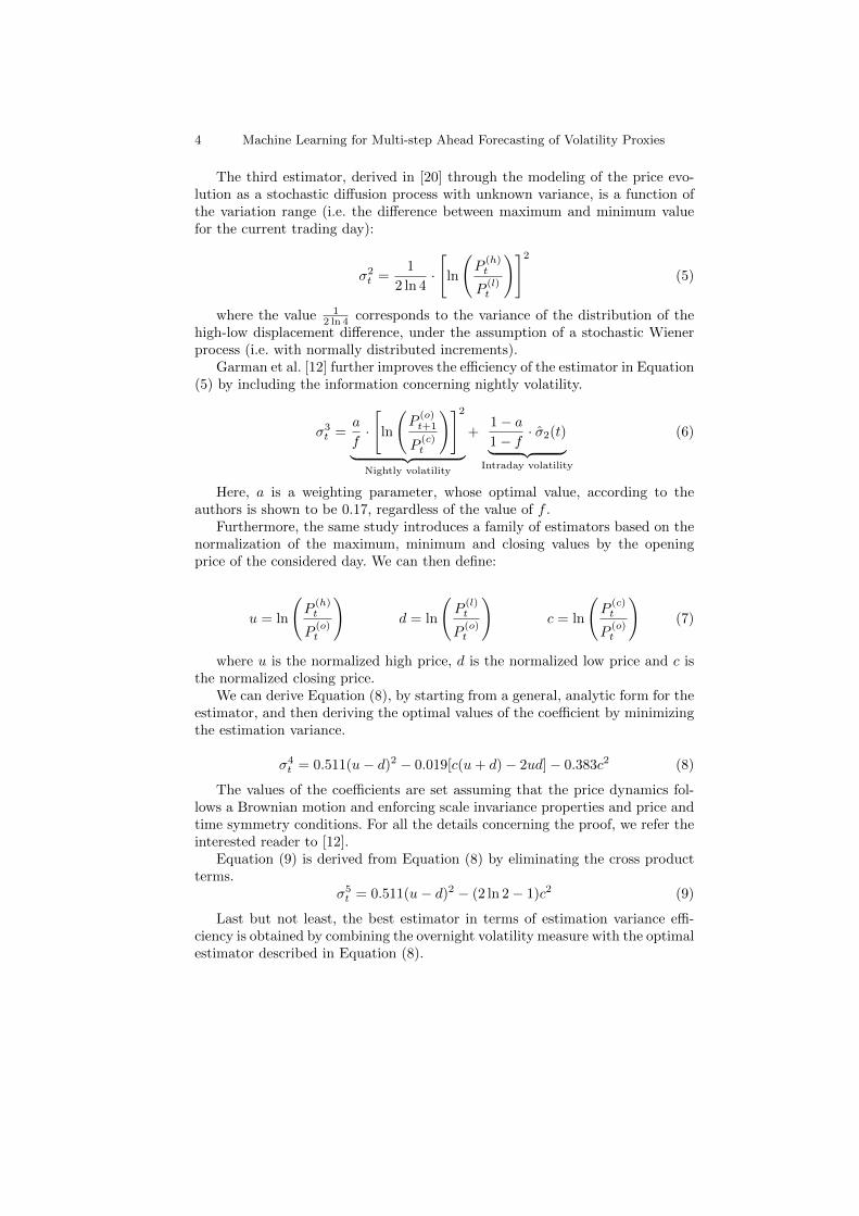
The third estimator, derived in [20] through the modeling of the price evo-lution as a stochastic diffusion process with unknown variance, is a function ofthe variation range (i.e. the difference between maximum and minimum valuefor the current trading day):

σ2t =

1

2 ln 4·

[ln

(P

(h)t

P(l)t

)]2(5)

where the value 12 ln 4 corresponds to the variance of the distribution of the

high-low displacement difference, under the assumption of a stochastic Wienerprocess (i.e. with normally distributed increments).

Garman et al. [12] further improves the efficiency of the estimator in Equation(5) by including the information concerning nightly volatility.

σ3t =

a

f·

[ln

(P

(o)t+1

P(c)t

)]2︸︷︷︸

Nightly volatility

+1− a1− f

· σ2(t)︸︷︷︸Intraday volatility

(6)

Here, a is a weighting parameter, whose optimal value, according to theauthors is shown to be 0.17, regardless of the value of f .

Furthermore, the same study introduces a family of estimators based on thenormalization of the maximum, minimum and closing values by the openingprice of the considered day. We can then define:

u = ln

(P

(h)t

P(o)t

)d = ln

(P

(l)t

P(o)t

)c = ln

(P

(c)t

P(o)t

)(7)

where u is the normalized high price, d is the normalized low price and c isthe normalized closing price.

We can derive Equation (8), by starting from a general, analytic form for theestimator, and then deriving the optimal values of the coefficient by minimizingthe estimation variance.

σ4t = 0.511(u− d)2 − 0.019[c(u+ d)− 2ud]− 0.383c2 (8)

The values of the coefficients are set assuming that the price dynamics fol-lows a Brownian motion and enforcing scale invariance properties and price andtime symmetry conditions. For all the details concerning the proof, we refer theinterested reader to [12].

Equation (9) is derived from Equation (8) by eliminating the cross productterms.

σ5t = 0.511(u− d)2 − (2 ln 2− 1)c2 (9)

Last but not least, the best estimator in terms of estimation variance effi-ciency is obtained by combining the overnight volatility measure with the optimalestimator described in Equation (8).


σ6t =

a

f· log

(P

(o)t+1

P(c)t

)2

︸︷︷︸Nightly volatility

+1− a1− f

· σ4(t)︸︷︷︸Intraday volatility

(10)

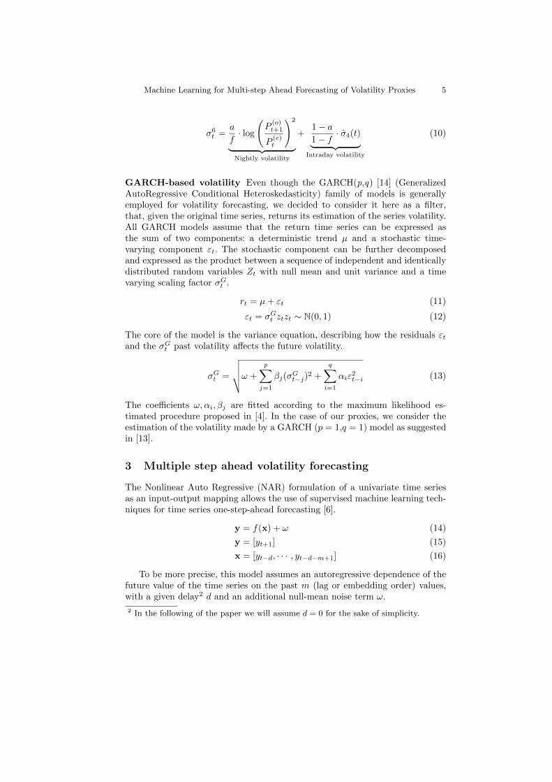
GARCH-based volatility Even though the GARCH(p,q) [14] (GeneralizedAutoRegressive Conditional Heteroskedasticity) family of models is generallyemployed for volatility forecasting, we decided to consider it here as a filter,that, given the original time series, returns its estimation of the series volatility.All GARCH models assume that the return time series can be expressed asthe sum of two components: a deterministic trend µ and a stochastic time-varying component εt. The stochastic component can be further decomposedand expressed as the product between a sequence of independent and identicallydistributed random variables Zt with null mean and unit variance and a timevarying scaling factor σG

t .

rt = µ+ εt (11)

εt = σGt ztzt ∼ N(0, 1) (12)

The core of the model is the variance equation, describing how the residuals εtand the σG

t past volatility affects the future volatility.

σGt =

√√√√ω +

p∑j=1

βj(σGt−j)

2 +

q∑i=1

αiε2t−i (13)

The coefficients ω, αi, βj are fitted according to the maximum likelihood es-timated procedure proposed in [4]. In the case of our proxies, we consider theestimation of the volatility made by a GARCH (p = 1,q = 1) model as suggestedin [13].

3 Multiple step ahead volatility forecasting

The Nonlinear Auto Regressive (NAR) formulation of a univariate time seriesas an input-output mapping allows the use of supervised machine learning tech-niques for time series one-step-ahead forecasting [6].

y = f(x) + ω (14)

y = [yt+1] (15)

x = [yt−d, · · · , yt−d−m+1] (16)

To be more precise, this model assumes an autoregressive dependence of thefuture value of the time series on the past m (lag or embedding order) values,with a given delay2 d and an additional null-mean noise term ω.

2 In the following of the paper we will assume d = 0 for the sake of simplicity.


With this structure, the forecasting task can be reduced to a two-step process.First the mapping f between the inputs x and the outputs y is learned througha supervised learning task, and then such mapping is used to produce the one-step-ahead forecast of the future values.

Extensions of this technique allows to perform multiple-step ahead forecast(i.e. y = [yt+H , · · · , yt+1]). Such extensions can be summarised into two mainclasses: single output (Direct and Recursive strategies) and multiple output(MIMO) strategies. The former learns a multi-input single output dependencywhile the latter learns a multi-input multiple output dependency. We invite theinterested reader to see [24], [6], [25] for more details.

In what follows, we focus on two multi-step ahead single output learningtask, employing the Direct strategy [5], [23], [8]. In the first one (NAR), we willfocus on the multiple step ahead forecast of a primary volatility proxy σP

t usingonly its past values as input information, while in the second one (NARX), alsothe past values of an additional volatility proxy σX

t will be incorporated in themodel described in (14):

yNAR = yNARX = [σPt+H , · · · , σP

t+1] (17)

xNAR = [σPt−d, · · · , σP

t−d−m+1] (18)

xNARX = [σPt−d, · · · , σP

t−d−m+1, σXt−d, · · · , σX

t−d−m+1] (19)

We compare the two approaches for embedding orders m ∈ {2, 5}, severalforecasting horizons h ∈ {2, 5, 8, 10, 12} and for different estimators of the de-pendency f . More precisely, as estimators of the dependency, we employ a naivemodel, a GARCH(1,1), and three machine learning approaches: a feedforwardArtificial Neural Networks, a k-Nearest Neighbors approach and Support VectorMachine based regression.

3.1 Naive

The Naive method is employed mainly as a benchmark for comparison for theother models, simply consisting in taking the last available historical value:

σPt+h = σP

t−1 (20)

3.2 GARCH(1,1)

The GARCH model corresponds to the one described in subsection 2, in equa-tions (13) and (11), with p = 1 and q = 1.

3.3 Artificial Neural Networks

In machine learning and cognitive science, an artificial neural network (ANN) is anetwork of interconnected processing elements, called neurons, which are used toestimate or approximate functions that can depend on a large number of inputs


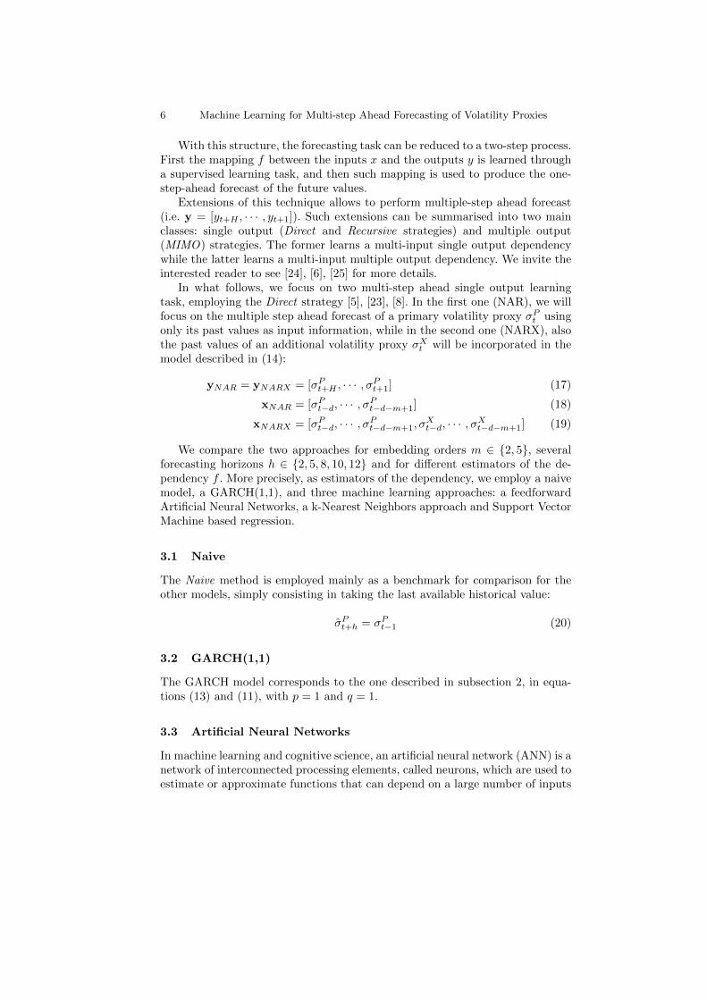
that are generally unknown. For our task, we will focus on a specific familyof artificial neural networks, the multi-layer perceptron (MLP), with a singlehidden layer. Equations (21) and (22) describe the structure of the model for asingle forecasting horizon t+h in the context of the Direct strategy, respectivelyfor a NAR and a NARX model.

It should be noted that, as shown in Equation (21), the model can be de-composed into a linear autoregressive component of order m and a nonlinearcomponent whose structure depends on the number of hidden nodes H (selectedthrough k-fold cross-validation). When an external regressor is added, its in-fluence will affect both the linear and nonlinear component, as shown in (22).In both cases the activity functions fho (·) and fh(·) are both logistic functions.Finally, our implementation of the MLP models is based on the nnet packagefor R [28].

σPt+h = fh

o

bo +

m∑i=1

wioσPt−i︸︷︷︸

Linear AR(m)

+

H∑j=1

wjo · fh

(m∑i=1

wijσPt−i + bj

)︸︷︷︸

Non-linear component

(21)

σPt+h = fh

o

bo

+

m∑i=1

wioσPt−i + w(i+m)oσ

Xt−i︸︷︷︸

Linear ARX(m)

+

H∑j=1

wjo · fh

(m∑i=1

wijσPt−i + w(i+m)jσ

Xt−i + bj

)︸︷︷︸

Non-linear component

(22)

3.4 K Nearest Neighbors

The k-Nearest neighbors (kNN) model is a local nonlinear model used for clas-sification and regression. In the case of regression, the prediction for a giveninput vector x∗ is obtained through local learning [3], a method that producespredictions by fitting a simple local model in the neighborhood of the point tobe predicted. The neighborhood of a point is defined by taking the the k valueshaving the minimal values for a chosen distance metric defined on the space ofthe input vector [1].

In this case, every data point is represented in the form (x,y) where x rep-resents the vector of input values and y the corresponding output vector, asdescribed in Figure 1. Then the prediction for an unknown input vector x∗ iscomputed as follows:

y(x∗) =1

k

∑i∈kNN

y(xi) (23)

where y(xi) is the output vector of the ith nearest neighbor of the inputvector x in the dataset. The choice of the optimal number of neighbors k will


be performed through automatic leave-one-out selection as described in [5]. Ourimplementation of the kNN models is based on the R package gbcode [7].

3.5 Support Vector Regression

Support Vector Regression is a regression methodology, based on the SupportVector Machine theoretical framework [9]. The key idea behind SVR is that theregression model can be expressed using a subset of the input training examples,called the support vectors. In more formal terms, the model (Equation (24)) isa linear combination over all the n support vector of a bivariate kernel functionk(·, ·) taking as inputs the data point x whose forecast is required and the ith

support vector xi. The coefficients αi, α∗i are determined through the minimiza-

tion of an empirical risk function (cf. [22]), solved as a continuous optimizationproblem.

y =

n∑i=1

(αi − α∗i )k(x,xi) (24)

k(x,xi) = e‖x−xi‖

2

2γ2 (25)

Among the different available kernel functions we employ the radial basis one(Equation(25)), for which the optimal value of the γ parameter is determinedthrough grid search. Here, the SVM implementation of the R package e1071

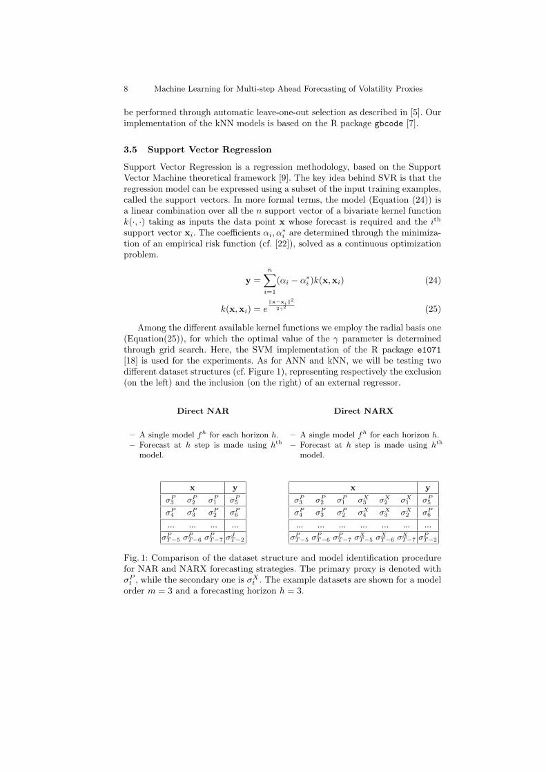
[18] is used for the experiments. As for ANN and kNN, we will be testing twodifferent dataset structures (cf. Figure 1), representing respectively the exclusion(on the left) and the inclusion (on the right) of an external regressor.

Direct NAR

– A single model fh for each horizon h.– Forecast at h step is made using hth

model.

x y

σP3 σP

2 σP1 σP

5

σP4 σP

3 σP2 σP

6

... ... ... ...

σPT−5 σ

PT−6 σ

PT−7 σ

JT−2

Direct NARX

– A single model fh for each horizon h.– Forecast at h step is made using hth

model.

x y

σP3 σP

2 σP1 σX

3 σX2 σX

1 σP5

σP4 σP

3 σP2 σX

4 σX3 σX

2 σP6

... ... ... ... ... ... ...

σPT−5 σ

PT−6 σ

PT−7 σ

XT−5 σ

XT−6 σ

XT−7 σ

PT−2

Fig. 1: Comparison of the dataset structure and model identification procedurefor NAR and NARX forecasting strategies. The primary proxy is denoted withσPt , while the secondary one is σX

t . The example datasets are shown for a modelorder m = 3 and a forecasting horizon h = 3.


4 Experimental Results

4.1 Dataset description

The proxies have been computed on the 40 time series of the french stock marketindex CAC40 from 05-01-2009 to 22-10-2014 (approximately 6 years) for a total1489 OHLC (Opening, High, Low, Closing) samples for each time series. Inaddition to the proxies, we include also the continuously compounded returnand the volume variable (representing the number of trades in given tradingday).

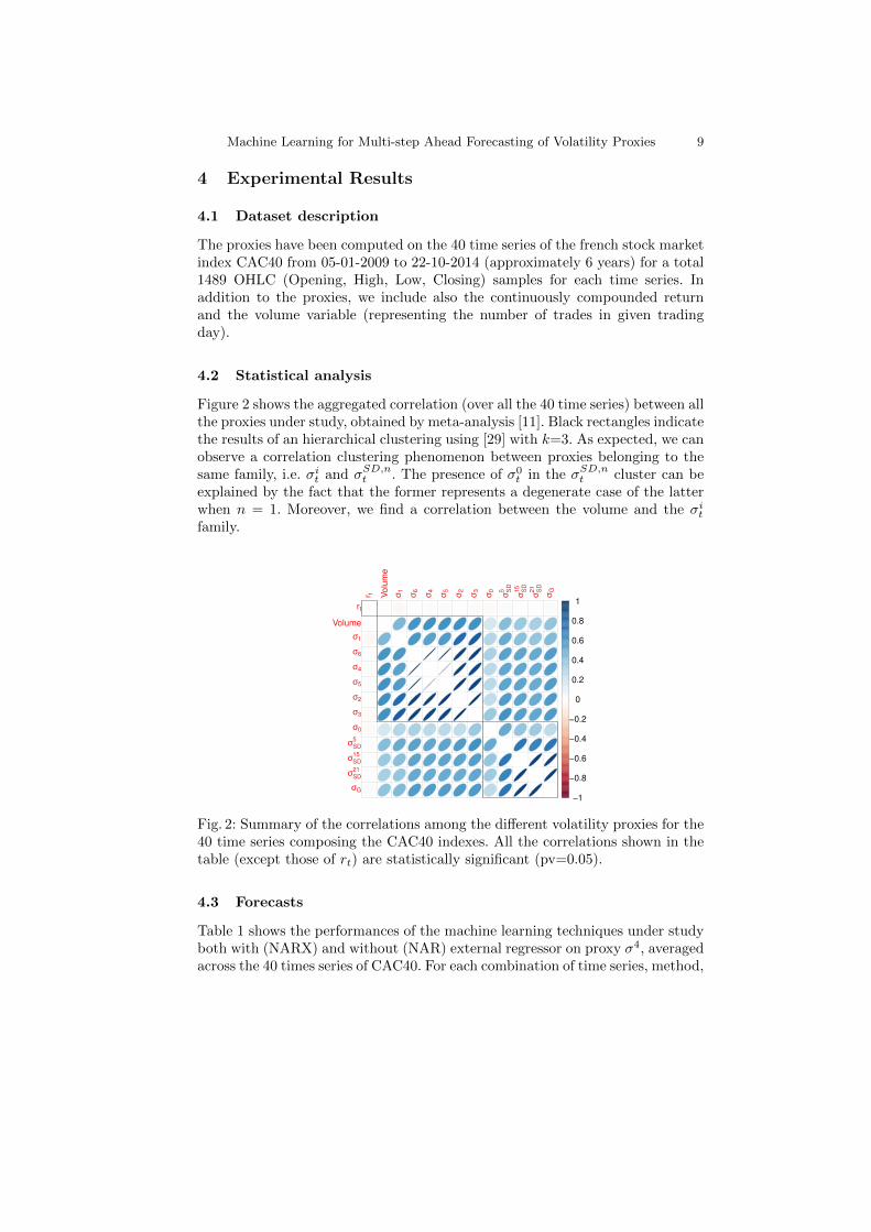
4.2 Statistical analysis

Figure 2 shows the aggregated correlation (over all the 40 time series) between allthe proxies under study, obtained by meta-analysis [11]. Black rectangles indicatethe results of an hierarchical clustering using [29] with k=3. As expected, we canobserve a correlation clustering phenomenon between proxies belonging to thesame family, i.e. σi

t and σSD,nt . The presence of σ0

t in the σSD,nt cluster can be

explained by the fact that the former represents a degenerate case of the latterwhen n = 1. Moreover, we find a correlation between the volume and the σi

t

family.

?

?

?

?

?

?

?

?

?

?

?

?

?

−1

−0.8

−0.6

−0.4

−0.2

0

0.2

0.4

0.6

0.8

1

r t Volu

me

σ 1 σ 6 σ 4 σ 5 σ 2 σ 3 σ 0 σ SD

5 σ SD

15

σ SD

21

σ G

rt

Volume

σ1

σ6

σ4

σ5

σ2

σ3

σ0

σSD

5

σSD

15

σSD

21

σG

Fig. 2: Summary of the correlations among the different volatility proxies for the40 time series composing the CAC40 indexes. All the correlations shown in thetable (except those of rt) are statistically significant (pv=0.05).

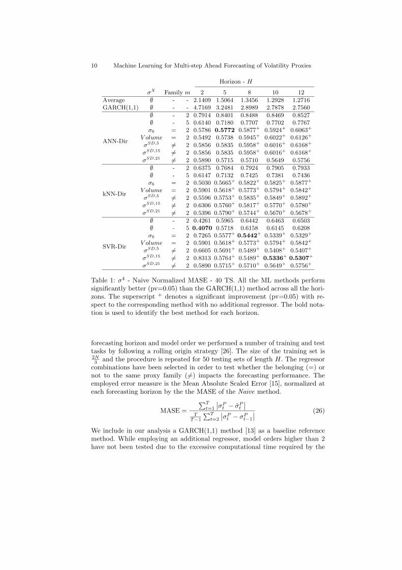
4.3 Forecasts

Table 1 shows the performances of the machine learning techniques under studyboth with (NARX) and without (NAR) external regressor on proxy σ4, averagedacross the 40 times series of CAC40. For each combination of time series, method,


Horizon - H

σX Family m 2 5 8 10 12

Average ∅ - - 2.1409 1.5064 1.3456 1.2928 1.2716GARCH(1,1) ∅ - - 4.7169 3.2481 2.8989 2.7878 2.7560

ANN-Dir

∅ - 2 0.7914 0.8401 0.8488 0.8469 0.8527∅ - 5 0.6140 0.7180 0.7707 0.7702 0.7767σ6 = 2 0.5786 0.5772 0.5877+ 0.5924+ 0.6063+

V olume = 2 0.5492 0.5738 0.5945+ 0.6022+ 0.6126+

σSD,5 6= 2 0.5856 0.5835 0.5958+ 0.6016+ 0.6168+

σSD,15 6= 2 0.5856 0.5835 0.5958+ 0.6016+ 0.6168+

σSD,21 6= 2 0.5890 0.5715 0.5710 0.5649 0.5756

kNN-Dir

∅ - 2 0.6375 0.7684 0.7924 0.7905 0.7933∅ - 5 0.6147 0.7132 0.7425 0.7381 0.7436σ6 = 2 0.5030 0.5665+ 0.5822+ 0.5825+ 0.5877+

V olume = 2 0.5901 0.5618+ 0.5773+ 0.5794+ 0.5842+

σSD,5 6= 2 0.5596 0.5753+ 0.5835+ 0.5849+ 0.5892+

σSD,15 6= 2 0.6306 0.5760+ 0.5817+ 0.5770+ 0.5780+

σSD,21 6= 2 0.5396 0.5790+ 0.5744+ 0.5670+ 0.5678+

SVR-Dir

∅ - 2 0.4261 0.5965 0.6442 0.6463 0.6503∅ - 5 0.4070 0.5718 0.6158 0.6145 0.6208σ6 = 2 0.7265 0.5577+ 0.5442+ 0.5339+ 0.5329+

V olume = 2 0.5901 0.5618+ 0.5773+ 0.5794+ 0.5842+

σSD,5 6= 2 0.6605 0.5691+ 0.5489+ 0.5408+ 0.5407+

σSD,15 6= 2 0.8313 0.5764+ 0.5489+ 0.5336+ 0.5307+

σSD,21 6= 2 0.5890 0.5715+ 0.5710+ 0.5649+ 0.5756+

Table 1: σ4 - Naive Normalized MASE - 40 TS. All the ML methods performsignificantly better (pv=0.05) than the GARCH(1,1) method across all the hori-zons. The superscript + denotes a significant improvement (pv=0.05) with re-spect to the corresponding method with no additional regressor. The bold nota-tion is used to identify the best method for each horizon.

forecasting horizon and model order we performed a number of training and testtasks by following a rolling origin strategy [26]. The size of the training set is2N3 and the procedure is repeated for 50 testing sets of length H. The regressor

combinations have been selected in order to test whether the belonging (=) ornot to the same proxy family ( 6=) impacts the forecasting performance. Theemployed error measure is the Mean Absolute Scaled Error [15], normalized ateach forecasting horizon by the the MASE of the Naive method.

MASE =

∑Tt=1

∣∣σPt − σP

t

∣∣T

T−1∑T

t=2

∣∣σPt − σP

t−1∣∣ (26)

We include in our analysis a GARCH(1,1) method [13] as a baseline referencemethod. While employing an additional regressor, model orders higher than 2have not been tested due to the excessive computational time required by the


corresponding technique for the given task or due to numerical convergenceproblems. A first observation from the table is that all the ML methods, bothin the single input and the multiple input configuration, are able to outperformthe reference GARCH method. Moreover, both the increase of the model or-der m and the introduction of an additional regressor are able to improve themethods’ performances. However, only the addition of an external regressor, forhorizons greater than 8 steps ahead is shown to bring a statistically significantimprovement (paired t-test, pv=0.05). Even though no model appear to clearlyoutperform all the others on every horizons, we can observe that the SVR modelfamily is generally able to produce smaller forecast errors than those based onANN and k-NN.

5 Conclusion and Future work

After having shown the benefits of including an additional proxies in our models,our main aim is to investigate how the forecasting quality of volatility could beimproved, mainly by tuning three parameters in our methods: the choice of theadditional proxy, the employed machine learning technique and the size of thetraining window. In order to further advance our research, we also plan to studyhow the current approach could be generalized, in order to include an arbitrarynumber of volatility proxies.

Acknowledgments. Jacopo De Stefani acknowledges the support of the ULB-WORLDLINE agreement. Gianluca Bontempi acknowledges the funding of theBrufence project (Scalable machine learning for automating defense system) sup-ported by INNOVIRIS (Brussels Institute for the encouragement of scientificresearch and innovation).

References

1. Altman, N.S.: An introduction to kernel and nearest-neighbor nonparametric re-gression. The American Statistician 46(3), 175–185 (1992)

2. Andersen, T.G., Bollerslev, T.: Arch and garch models. Encyclopedia of StatisticalSciences (1998)

3. Atkeson, C.G., Moore, A.W., Schaal, S.: Locally weighted learning for control. In:Lazy learning, pp. 75–113. Springer (1997)

4. Bollerslev, T.: Generalized autoregressive conditional heteroskedasticity. Journalof econometrics 31(3), 307–327 (1986)

5. Bontempi, G., Taieb, S.B.: Conditionally dependent strategies for multiple-step-ahead prediction in local learning. International journal of forecasting 27(3), 689–699 (2011)

6. Bontempi, G., Taieb, S.B., Le Borgne, Y.A.: Machine learning strategies for timeseries forecasting. In: Business Intelligence, pp. 62–77. Springer (2013)

7. Bontempi, Gianluca: Code from the handbook ”statistical foundations of machinelearning”, https://github.com/gbonte/gbcode


8. Cheng, H., Tan, P.N., Gao, J., Scripps, J.: Multistep-ahead time series prediction.In: Pacific-Asia Conference on Knowledge Discovery and Data Mining. pp. 765–774. Springer (2006)

9. Cortes, C., Vapnik, V.: Support vector machine. Machine learning 20(3), 273–297(1995)

10. Dash, R., Dash, P.: An evolutionary hybrid fuzzy computationally efficient egarchmodel for volatility prediction. Applied Soft Computing 45, 40–60 (2016)

11. Field, A.P.: Meta-analysis of correlation coefficients: a monte carlo comparison offixed-and random-effects methods. Psychological methods 6(2), 161 (2001)

12. Garman, M.B., Klass, M.J.: On the estimation of security price volatilities fromhistorical data. Journal of business pp. 67–78 (1980)

13. Hansen, P.R., Lunde, A.: A forecast comparison of volatility models: does anythingbeat a garch (1, 1)? Journal of applied econometrics 20(7), 873–889 (2005)

14. Hentschel, L.: All in the family nesting symmetric and asymmetric garch models.Journal of Financial Economics 39(1), 71–104 (1995)

15. Hyndman, R.J., Koehler, A.B.: Another look at measures of forecast accuracy.International journal of forecasting 22(4), 679–688 (2006)

16. Kristjanpoller, W., Fadic, A., Minutolo, M.C.: Volatility forecast using hybrid neu-ral network models. Expert Systems with Applications 41(5), 2437–2442 (2014)

17. Martens, M.: Measuring and forecasting s&p 500 index-futures volatility usinghigh-frequency data. Journal of Futures Markets 22(6), 497–518 (2002)

18. Meyer, D., Dimitriadou, E., Hornik, K., Weingessel, A., Leisch, F., Chang, C.C.,Lin, C.C.: e1071: Misc functions of the department of statistics, probability theorygroup (formerly: E1071), tu wien, https://cran.r-project.org/web/packages/e1071/

19. Monfared, S.A., Enke, D.: Volatility forecasting using a hybrid gjr-garch neuralnetwork model. Procedia Computer Science 36, 246–253 (2014)

20. Parkinson, M.: The extreme value method for estimating the variance of the rateof return. Journal of Business pp. 61–65 (1980)

21. Poon, S.H., Granger, C.W.: Forecasting volatility in financial markets: A review.Journal of economic literature 41(2), 478–539 (2003)

22. Sapankevych, N.I., Sankar, R.: Time series prediction using support vector ma-chines: a survey. IEEE Computational Intelligence Magazine 4(2) (2009)

23. Sorjamaa, A., Hao, J., Reyhani, N., Ji, Y., Lendasse, A.: Methodology for long-termprediction of time series. Neurocomputing 70(16), 2861–2869 (2007)

24. Taieb, S.B., Bontempi, G., Atiya, A.F., Sorjamaa, A.: A review and comparison ofstrategies for multi-step ahead time series forecasting based on the nn5 forecastingcompetition. Expert systems with applications 39(8), 7067–7083 (2012)

25. Taieb, S.B., Sorjamaa, A., Bontempi, G.: Multiple-output modeling for multi-step-ahead time series forecasting. Neurocomputing 73(10), 1950–1957 (2010)

26. Tashman, L.J.: Out-of-sample tests of forecasting accuracy: an analysis and review.International journal of forecasting 16(4), 437–450 (2000)

27. Tsay, R.S.: Analysis of financial time series, vol. 543. John Wiley & Sons (2005)28. Venables, W.N., Ripley, B.D.: Modern Applied Statistics with S. Springer, New

York, fourth edn. (2002), http://www.stats.ox.ac.uk/pub/MASS4, iSBN 0-387-95457-0

29. Ward Jr, J.H.: Hierarchical grouping to optimize an objective function. Journal ofthe American statistical association 58(301), 236–244 (1963)

30. Xiong, R., Nichols, E.P., Shen, Y.: Deep learning stock volatility with google do-mestic trends. arXiv preprint arXiv:1512.04916 (2015)

Documents

Machine Learning for Multi-step Ahead Forecasting of Volatility Proxiesceur-ws.org/Vol-1941/MIDAS2017_paper3.pdf · Machine Learning for Multi-step Ahead Forecasting of Volatility