Embed Size (px)
Citation preview
MMACROECONOMICSACROECONOMICS
C H A P T E R
© 2008 Worth Publishers, all rights reserved
SIXTH EDITIONSIXTH EDITION
PowerPointPowerPoint®® Slides by Ron Cronovich Slides by Ron CronovichNN. . GGREGORY REGORY MMANKIWANKIW
Economic Growth I: Capital Accumulation and Population Growth
7
CHAPTER 7 Economic Growth I slide 2
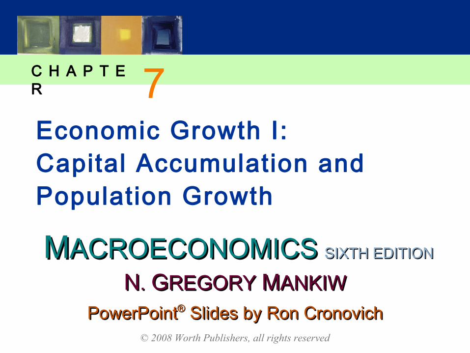
In this chapter, you wil l learn…
the closed economy Solow model
how a country’s standard of living depends on its saving and population growth rates
how to use the “Golden Rule” to find the optimal saving rate and capital stock
CHAPTER 7 Economic Growth I slide 3
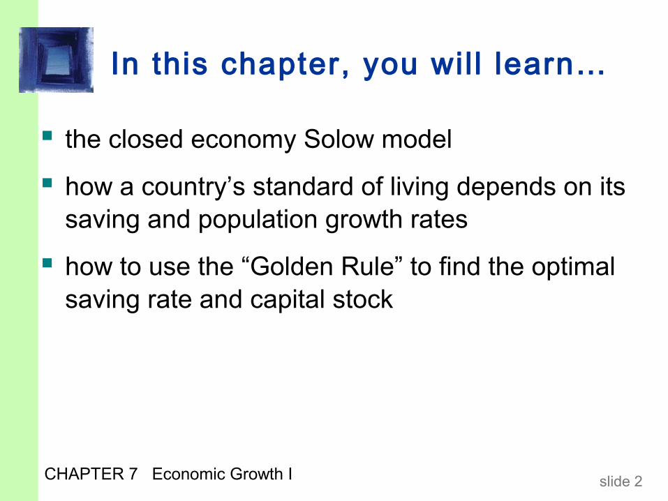
Why growth matters Data on infant mortality rates:
20% in the poorest 1/5 of all countries
0.4% in the richest 1/5
In Pakistan, 85% of people live on less than $2/day.
One-fourth of the poorest countries have had famines during the past 3 decades.
Poverty is associated with oppression of women and minorities.
Economic growth raises living standards and reduces poverty….
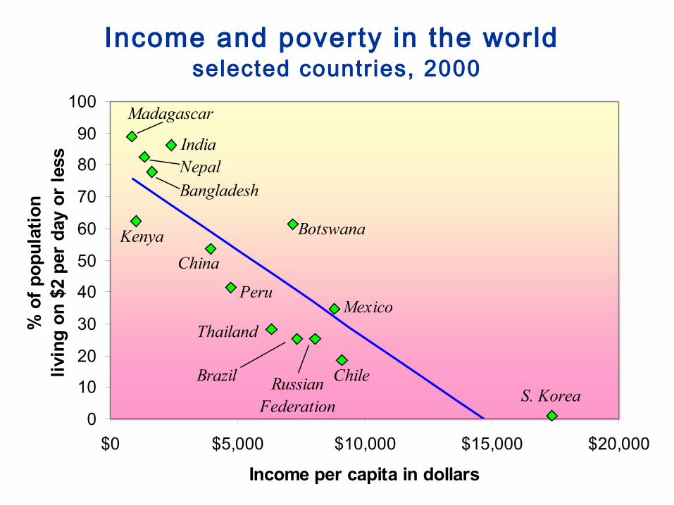
Income and poverty in the world selected countries, 2000
0
10
20
30
40
50
60
70
80
90
100
$0 $5,000 $10,000 $15,000 $20,000
Income per capita in dollars
% o
f p
op
ula
tio
n
livi
ng
on
$2
per
day
or
less
Madagascar
India
BangladeshNepal
Botswana
Mexico
ChileS. Korea
Brazil Russian Federation
Thailand
Peru
China
Kenya
CHAPTER 7 Economic Growth I slide 5
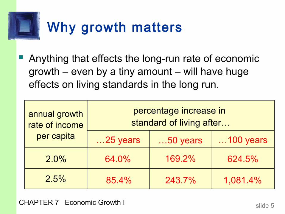
Why growth matters
Anything that effects the long-run rate of economic growth – even by a tiny amount – will have huge effects on living standards in the long run.
1,081.4%243.7%85.4%
624.5%169.2%64.0%
2.5%
2.0%
…100 years…50 years…25 years
percentage increase in standard of living after…
annual growth rate of income
per capita
CHAPTER 7 Economic Growth I slide 6
Why growth matters
If the annual growth rate of U.S. real GDP per capita had been just one-tenth of one percent higher during the 1990s, the U.S. would have generated an additional $496 billion of income during that decade.

CHAPTER 7 Economic Growth I slide 7
The lessons of growth theory…can make a positive difference in the lives of hundreds of millions of people.
These lessons help us
understand why poor countries are poor
design policies that can help them grow
learn how our own growth rate is affected by shocks and our government’s policies
CHAPTER 7 Economic Growth I slide 8
The Solow model
due to Robert Solow,won Nobel Prize for contributions to the study of economic growth
a major paradigm: widely used in policy making
benchmark against which most recent growth theories are compared
looks at the determinants of economic growth and the standard of living in the long run
CHAPTER 7 Economic Growth I slide 9
How Solow model is different from Chapter 3’s model
1. K is no longer fixed:investment causes it to grow, depreciation causes it to shrink
2. L is no longer fixed:population growth causes it to grow
3. the consumption function is simpler
CHAPTER 7 Economic Growth I slide 10
How Solow model is different from Chapter 3’s model
4. no G or T(only to simplify presentation; we can still do fiscal policy experiments)
5. cosmetic differences
CHAPTER 7 Economic Growth I slide 11
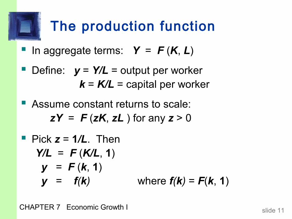
The production function
In aggregate terms: Y = F (K, L)
Define: y = Y/L = output per worker k = K/L = capital per worker
Assume constant returns to scale:zY = F (zK, zL ) for any z > 0
Pick z = 1/L. Then Y/L = F (K/L, 1) y = F (k, 1) y = f(k) where f(k) = F(k, 1)

CHAPTER 7 Economic Growth I slide 12
The production functionOutput per worker, y
Capital per worker, k
f(k)
Note: this production function exhibits diminishing MPK.
Note: this production function exhibits diminishing MPK.
1MPK = f(k +1) – f(k)
CHAPTER 7 Economic Growth I slide 13
The national income identity
Y = C + I (remember, no G )
In “per worker” terms: y = c + i where c = C/L and i = I /L
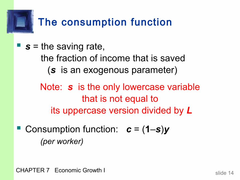
CHAPTER 7 Economic Growth I slide 14
The consumption function
s = the saving rate, the fraction of income that is saved
(s is an exogenous parameter)
Note: s is the only lowercase variable that is not equal to
its uppercase version divided by L
Consumption function: c = (1–s)y (per worker)
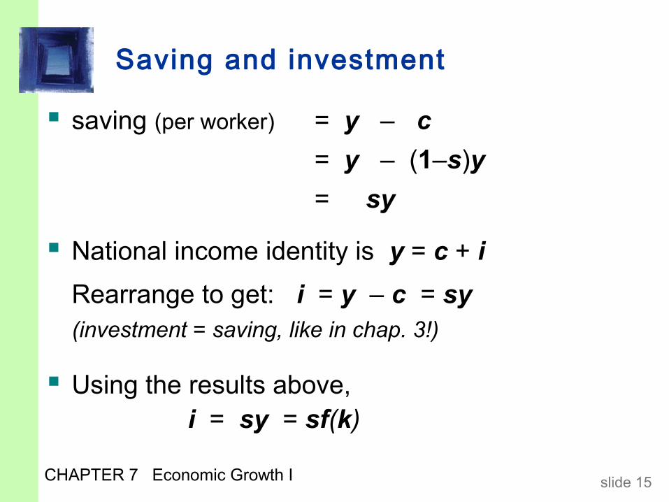
CHAPTER 7 Economic Growth I slide 15
Saving and investment
saving (per worker) = y – c
= y – (1–s)y
= sy
National income identity is y = c + i
Rearrange to get: i = y – c = sy
(investment = saving, like in chap. 3!)
Using the results above, i = sy = sf(k)
CHAPTER 7 Economic Growth I slide 16
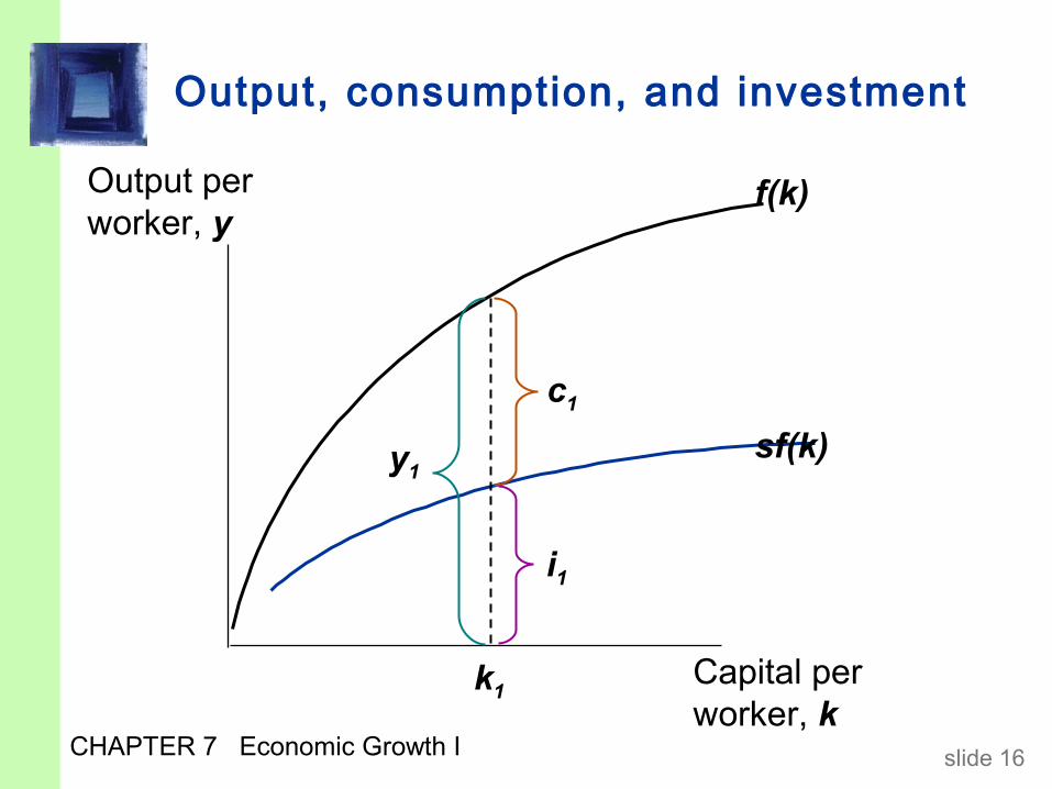
Output, consumption, and investment
Output per worker, y
Capital per worker, k
f(k)
sf(k)
k1
y1
i1
c1
CHAPTER 7 Economic Growth I slide 17
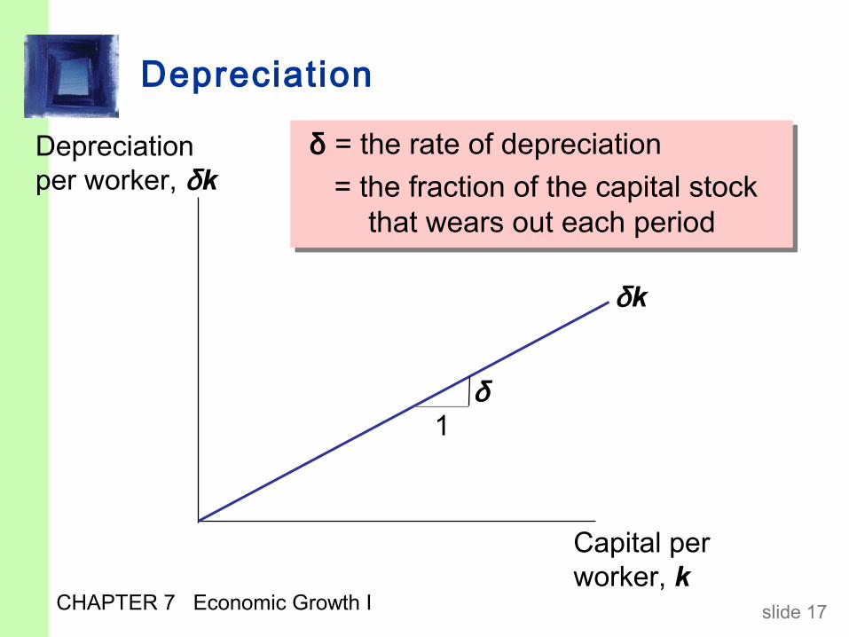
Depreciation
Depreciation per worker, δk
Capital per worker, k
δk
δ = the rate of depreciation
= the fraction of the capital stock that wears out each period
δ = the rate of depreciation
= the fraction of the capital stock that wears out each period
1δ
CHAPTER 7 Economic Growth I slide 18
Capital accumulation
Change in capital stock = investment – depreciation∆k = i – δk
Since i = sf(k) , this becomes:
∆k = s f(k) – δk
The basic idea: Investment increases the capital stock, depreciation reduces it.
CHAPTER 7 Economic Growth I slide 19
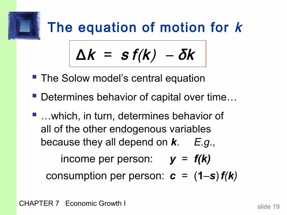
The equation of motion for k
The Solow model’s central equation
Determines behavior of capital over time…
…which, in turn, determines behavior of all of the other endogenous variables because they all depend on k. E.g.,
income per person: y = f(k)
consumption per person: c = (1–s) f(k)
∆k = s f(k) – δk
CHAPTER 7 Economic Growth I slide 20
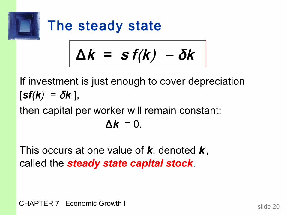
The steady state
If investment is just enough to cover depreciation [sf(k) = δk ],
then capital per worker will remain constant: ∆k = 0.
This occurs at one value of k, denoted k*, called the steady state capital stock.
∆k = s f(k) – δk
CHAPTER 7 Economic Growth I slide 21
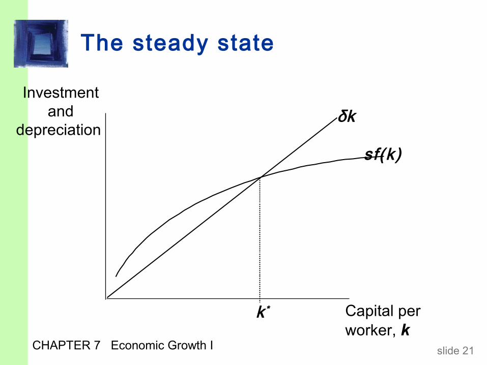
The steady state
Investment and
depreciation
Capital per worker, k
sf(k)
δk
k *
CHAPTER 7 Economic Growth I slide 22
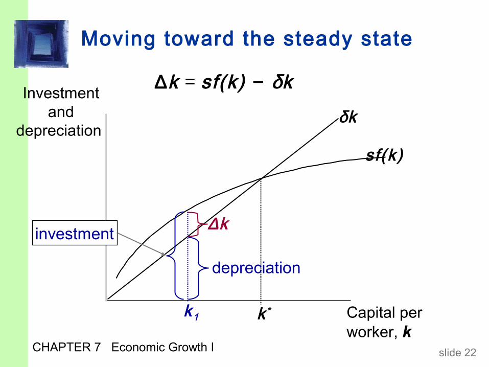
Moving toward the steady state
Investment and
depreciation
Capital per worker, k
sf(k)
δk
k *
∆k = sf(k) − δk
depreciation
∆k
k1
investment
CHAPTER 7 Economic Growth I slide 24
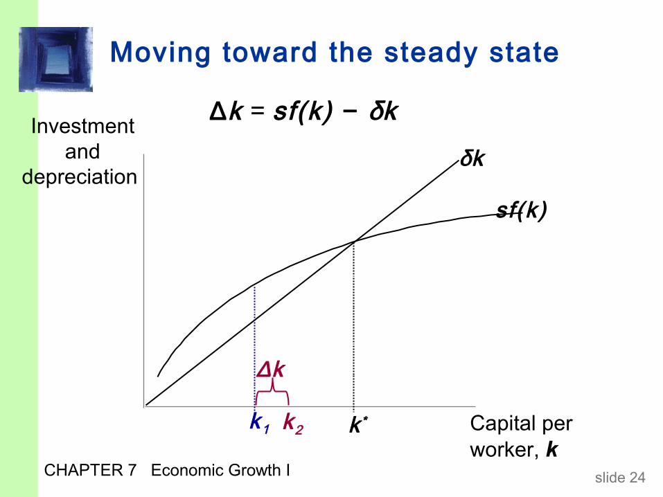
Moving toward the steady state
Investment and
depreciation
Capital per worker, k
sf(k)
δk
k * k1
∆k = sf(k) − δk
∆k
k2
CHAPTER 7 Economic Growth I slide 25
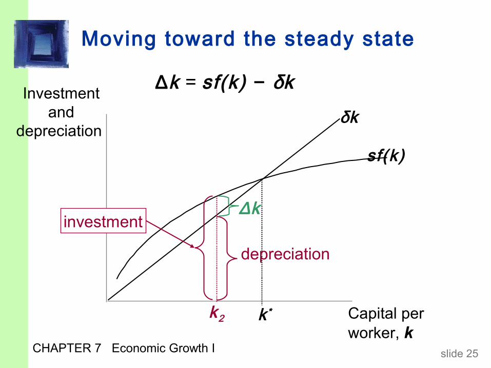
Moving toward the steady state
Investment and
depreciation
Capital per worker, k
sf(k)
δk
k *
∆k = sf(k) − δk
k2
investment
depreciation
∆k
CHAPTER 7 Economic Growth I slide 27
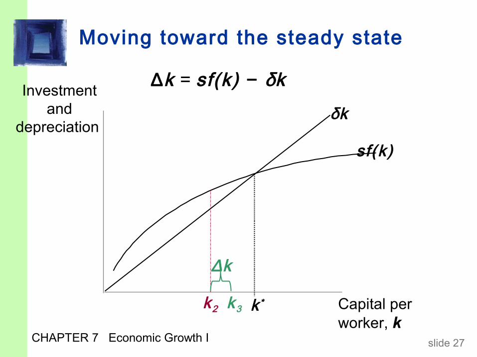
Moving toward the steady state
Investment and
depreciation
Capital per worker, k
sf(k)
δk
k *
∆k = sf(k) − δk
k2
∆k
k3
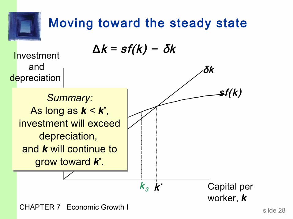
CHAPTER 7 Economic Growth I slide 28
Moving toward the steady state
Investment and
depreciation
Capital per worker, k
sf(k)
δk
k *
∆k = sf(k) − δk
k3
Summary:As long as k < k*,
investment will exceed depreciation,
and k will continue to grow toward k*.
Summary:As long as k < k*,
investment will exceed depreciation,
and k will continue to grow toward k*.
CHAPTER 7 Economic Growth I slide 29
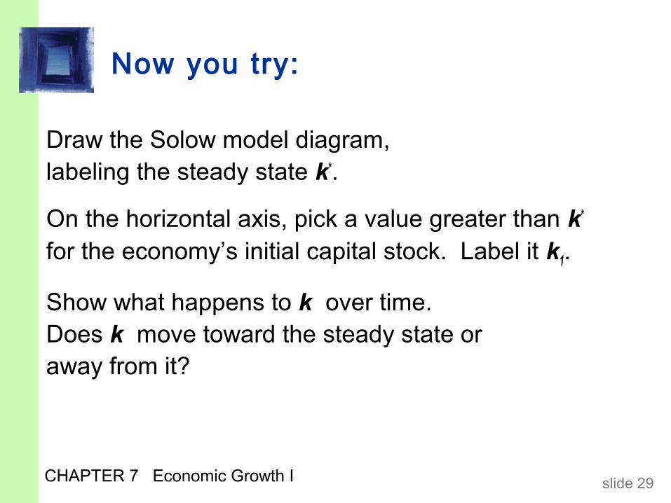
Now you try:
Draw the Solow model diagram, labeling the steady state k*.
On the horizontal axis, pick a value greater than k*
for the economy’s initial capital stock. Label it k1.
Show what happens to k over time. Does k move toward the steady state or away from it?
CHAPTER 7 Economic Growth I slide 30
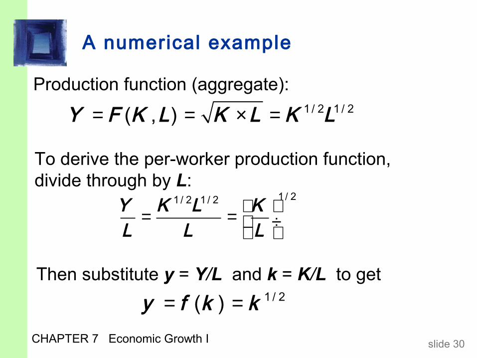
A numerical example
Production function (aggregate):
= = × = 1 / 2 1 / 2( , )Y F K L K L K L
= = ÷
1 / 21 / 2 1 / 2Y K L KL L L
= = 1 / 2( )y f k k
To derive the per-worker production function, divide through by L:
Then substitute y = Y/L and k = K/L to get
CHAPTER 7 Economic Growth I slide 31
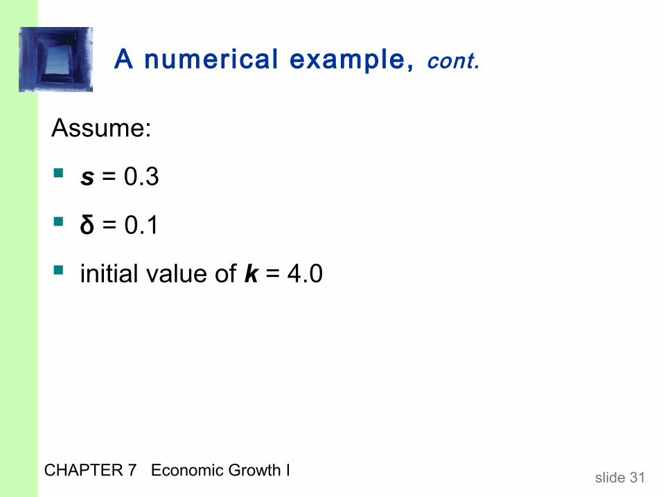
A numerical example, cont.
Assume:
s = 0.3
δ = 0.1
initial value of k = 4.0
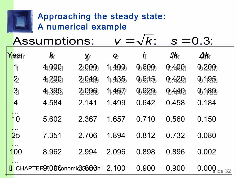
CHAPTER 7 Economic Growth I slide 32
Approaching the steady state: A numerical example
Year k y c i k ∆k
1 4.000 2.000 1.400 0.600 0.400 0.200
2 4.200 2.049 1.435 0.615 0.420 0.195
3 4.395 2.096 1.467 0.629 0.440 0.189
Year k y c i k ∆k
1 4.000 2.000 1.400 0.600 0.400 0.200
2 4.200 2.049 1.435 0.615 0.420 0.195
3 4.395 2.096 1.467 0.629 0.440 0.189
Assumptions: ; 0.3; 0.1; initial 4.0y k s kδ= = = =
4 4.584 2.141 1.499 0.642 0.458 0.184 … 10 5.602 2.367 1.657 0.710 0.560 0.150 … 25 7.351 2.706 1.894 0.812 0.732 0.080 … 100 8.962 2.994 2.096 0.898 0.896 0.002 … 9.000 3.000 2.100 0.900 0.900 0.000
CHAPTER 7 Economic Growth I slide 33
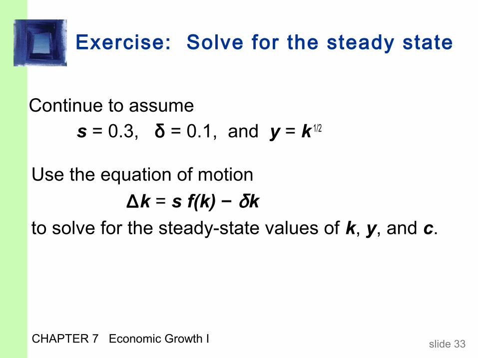
Exercise: Solve for the steady state
Continue to assume s = 0.3, δ = 0.1, and y = k 1/2
Use the equation of motion
∆k = s f(k) − δk
to solve for the steady-state values of k, y, and c.
CHAPTER 7 Economic Growth I slide 34
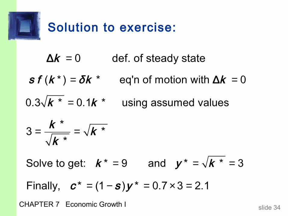
Solution to exercise:
def. of steady statek = 0∆
and y k= =* * 3
eq'n of motion with s f k k kδ= =( * ) * 0∆
using assumed valuesk k=0.3 * 0.1 *
*3 * *
k kk
= =
Solve to get: k =* 9
Finally, c s y= − = × =* (1 ) * 0.7 3 2.1
CHAPTER 7 Economic Growth I slide 35
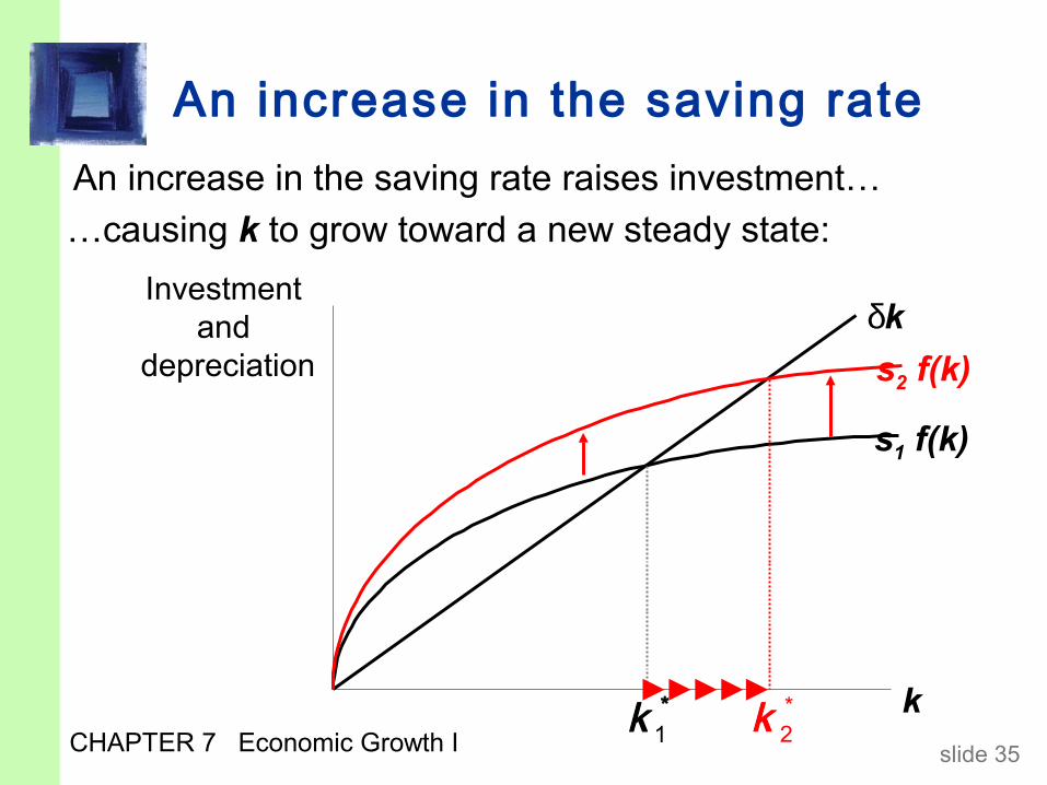
An increase in the saving rate
Investment and
depreciation
k
δk
s1 f(k)
*k 1
An increase in the saving rate raises investment…
…causing k to grow toward a new steady state:
s2 f(k)
*k 2
CHAPTER 7 Economic Growth I slide 36
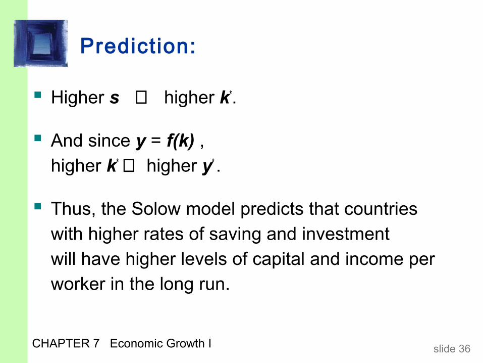
Prediction:
Higher s ⇒ higher k*.
And since y = f(k) , higher k* ⇒ higher y* .
Thus, the Solow model predicts that countries with higher rates of saving and investment will have higher levels of capital and income per worker in the long run.
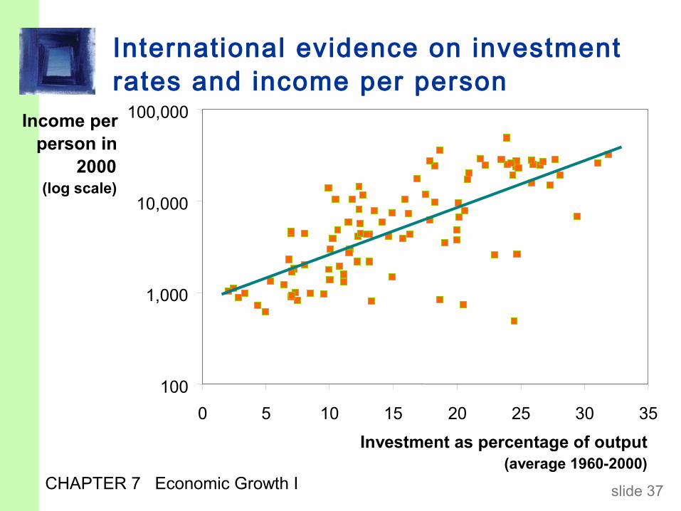
CHAPTER 7 Economic Growth I slide 37
International evidence on investment rates and income per person
100
1,000
10,000
100,000
0 5 10 15 20 25 30 35
Investment as percentage of output (average 1960-2000)
Income per person in
2000 (log scale)
CHAPTER 7 Economic Growth I slide 38
The Golden Rule: Introduction
Different values of s lead to different steady states. How do we know which is the “best” steady state?
The “best” steady state has the highest possible consumption per person: c* = (1–s) f(k*).
An increase in s
leads to higher k* and y*, which raises c*
reduces consumption’s share of income (1–s), which lowers c*.
So, how do we find the s and k* that maximize c*?
CHAPTER 7 Economic Growth I slide 39
The Golden Rule capital stock
the Golden Rule level of capital, the steady state value of k
that maximizes consumption.
*goldk =
To find it, first express c* in terms of k*:
c* = y* − i*
= f (k*) − i*
= f (k*) − δk* In the steady state:
i* = δk* because ∆k = 0.
CHAPTER 7 Economic Growth I slide 40
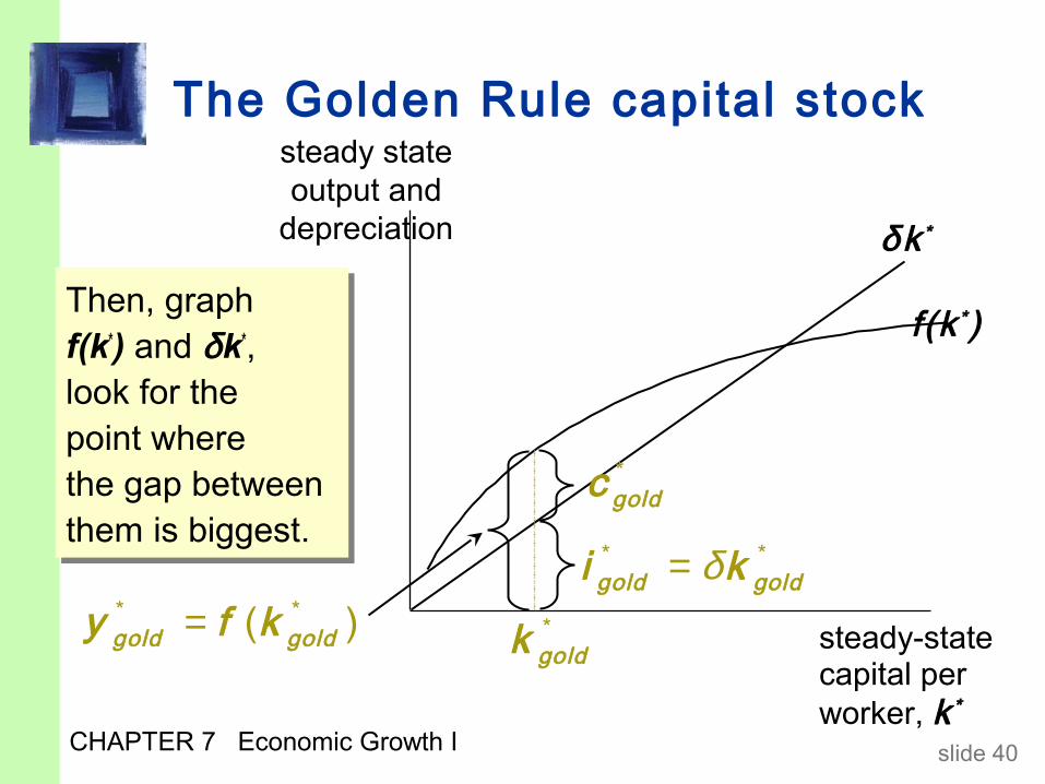
Then, graph f(k*) and δk*, look for the point where the gap between them is biggest.
Then, graph f(k*) and δk*, look for the point where the gap between them is biggest.
The Golden Rule capital stocksteady state output and
depreciation
steady-state capital per worker, k *
f(k *)
δ k *
*goldk
*goldc
* *gold goldi kδ=
* *( )gold goldy f k=
CHAPTER 7 Economic Growth I slide 41
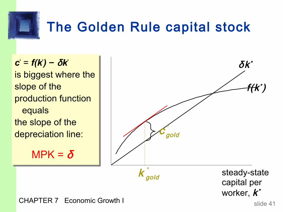
The Golden Rule capital stock
c* = f(k*) − δk*
is biggest where the slope of the production function equals the slope of the depreciation line:
c* = f(k*) − δk*
is biggest where the slope of the production function equals the slope of the depreciation line:
steady-state capital per worker, k *
f(k *)
δ k *
*goldk
*goldc
MPK = δ
CHAPTER 7 Economic Growth I slide 42
The transit ion to the Golden Rule steady state
The economy does NOT have a tendency to move toward the Golden Rule steady state.
Achieving the Golden Rule requires that policymakers adjust s.
This adjustment leads to a new steady state with higher consumption.
But what happens to consumption during the transition to the Golden Rule?
CHAPTER 7 Economic Growth I slide 43
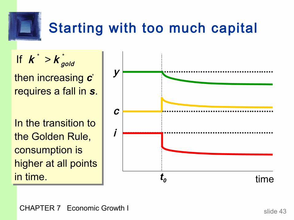
Starting with too much capital
then increasing c* requires a fall in s.
In the transition to the Golden Rule, consumption is higher at all points in time.
then increasing c* requires a fall in s.
In the transition to the Golden Rule, consumption is higher at all points in time.
If goldk k>* *
timet0
c
i
y
CHAPTER 7 Economic Growth I slide 44
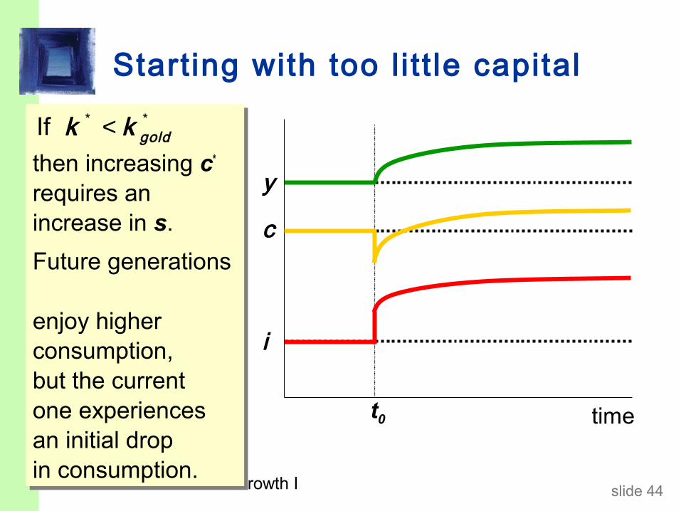
Starting with too l i t t le capital
then increasing c* requires an increase in s.
Future generations
enjoy higher consumption, but the current one experiences an initial drop in consumption.
then increasing c* requires an increase in s.
Future generations
enjoy higher consumption, but the current one experiences an initial drop in consumption.
If goldk k<* *
timet0
c
i
y
CHAPTER 7 Economic Growth I slide 45
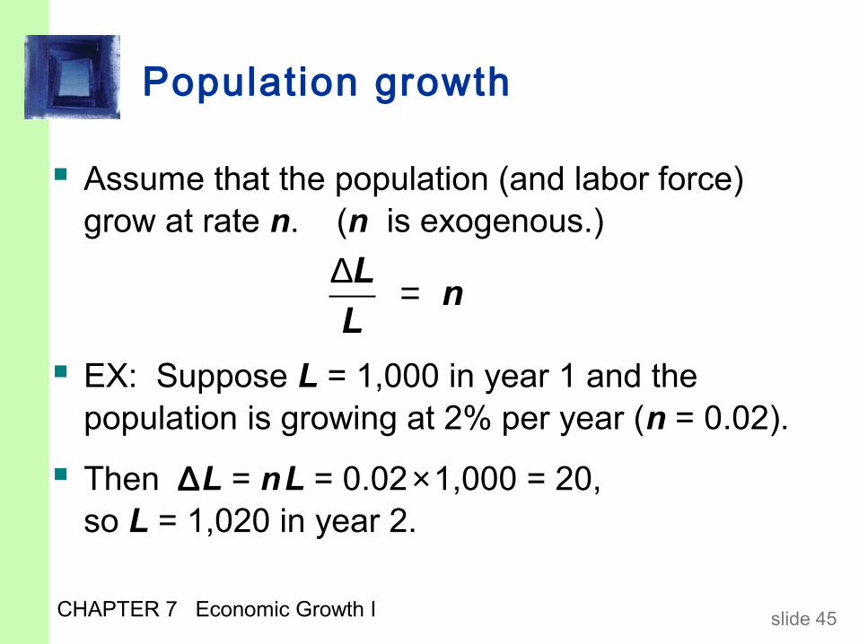
Population growth
Assume that the population (and labor force) grow at rate n. (n is exogenous.)
EX: Suppose L = 1,000 in year 1 and the population is growing at 2% per year (n = 0.02).
Then ∆L = n L = 0.02 × 1,000 = 20,so L = 1,020 in year 2.
∆ =Ln
L
CHAPTER 7 Economic Growth I slide 46
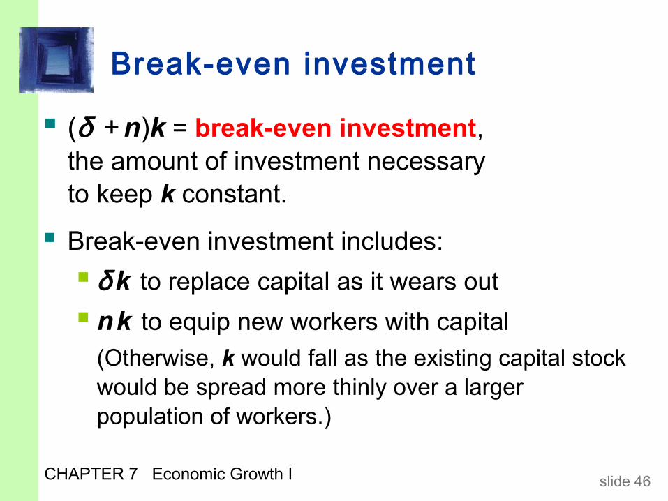
Break-even investment
(δ + n)k = break-even investment, the amount of investment necessary to keep k constant.
Break-even investment includes:
δ k to replace capital as it wears out
n k to equip new workers with capital
(Otherwise, k would fall as the existing capital stock would be spread more thinly over a larger population of workers.)
CHAPTER 7 Economic Growth I slide 47
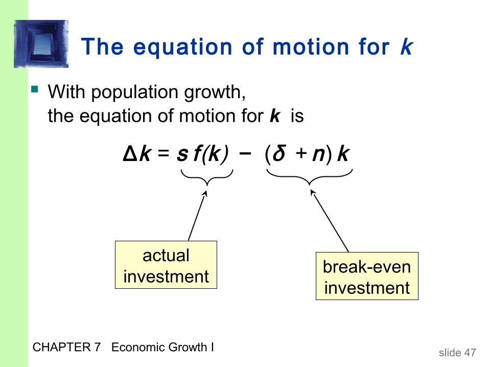
The equation of motion for k
With population growth, the equation of motion for k is
break-even investment
actual investment
∆k = s f(k) − (δ + n) k
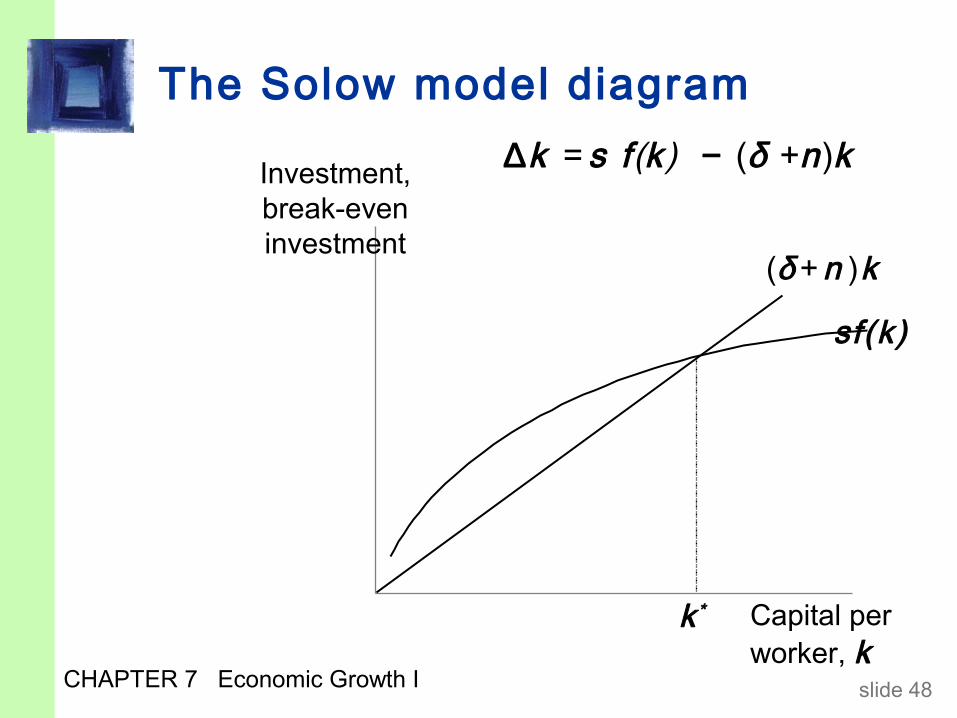
CHAPTER 7 Economic Growth I slide 48
The Solow model diagram
Investment, break-even investment
Capital per worker, k
sf(k)
(δ + n ) k
k *
∆k = s f(k) − (δ +n)k

CHAPTER 7 Economic Growth I slide 49
The impact of population growth
Investment, break-even investment
Capital per worker, k
sf(k)
(δ +n1) k
k1*
(δ +n2) k
k2*
An increase in n causes an increase in break-even investment,
An increase in n causes an increase in break-even investment,leading to a lower steady-state level of k.
CHAPTER 7 Economic Growth I slide 50
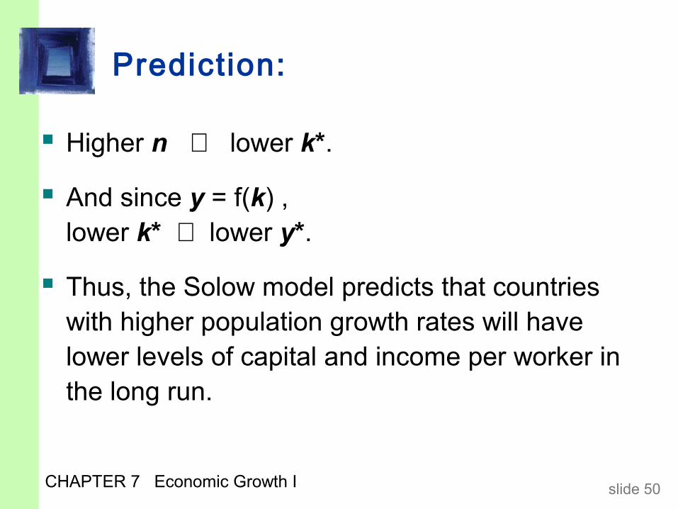
Prediction:
Higher n ⇒ lower k*.
And since y = f(k) , lower k* ⇒ lower y*.
Thus, the Solow model predicts that countries with higher population growth rates will have lower levels of capital and income per worker in the long run.
CHAPTER 7 Economic Growth I slide 51
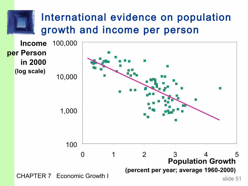
International evidence on population growth and income per person
100
1,000
10,000
100,000
0 1 2 3 4 5Population Growth
(percent per year; average 1960-2000)
Income per Person
in 2000 (log scale)
CHAPTER 7 Economic Growth I slide 52
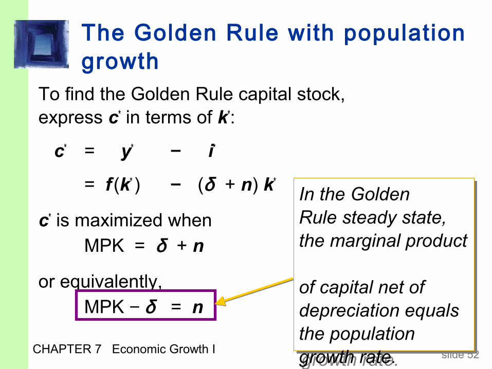
The Golden Rule with population growth
To find the Golden Rule capital stock, express c* in terms of k*:
c* = y* − i*
= f (k* ) − (δ + n) k*
c* is maximized when MPK = δ + n
or equivalently, MPK − δ = n
In the Golden Rule steady state, the marginal product
of capital net of depreciation equals the population growth rate.
In the Golden Rule steady state, the marginal product
of capital net of depreciation equals the population growth rate.
CHAPTER 7 Economic Growth I slide 53
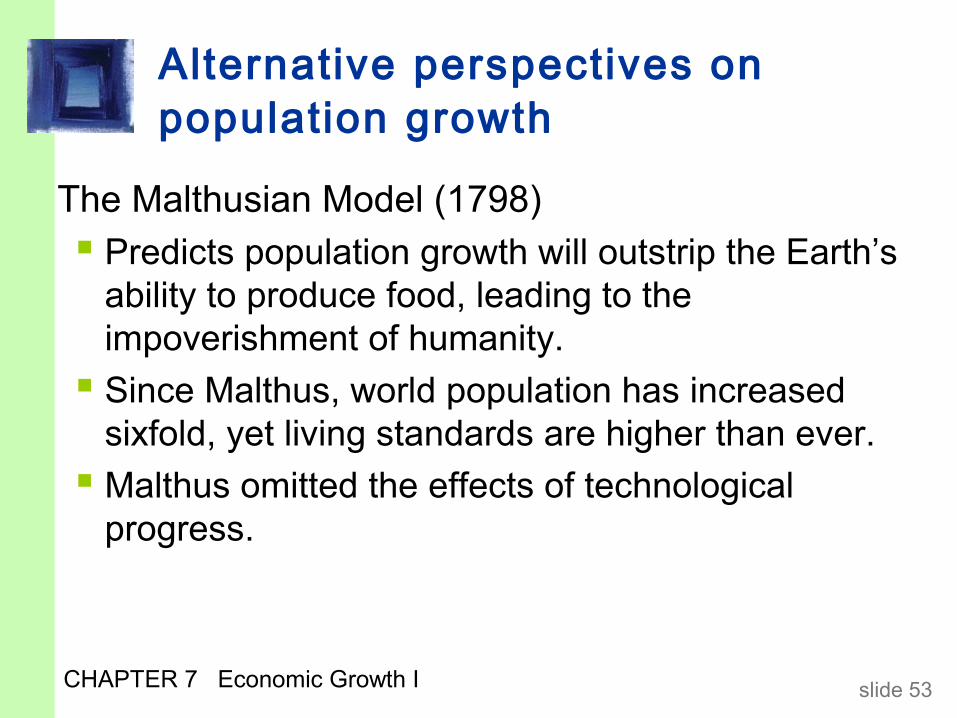
Alternative perspectives on population growth
The Malthusian Model (1798) Predicts population growth will outstrip the Earth’s
ability to produce food, leading to the impoverishment of humanity.
Since Malthus, world population has increased sixfold, yet living standards are higher than ever.
Malthus omitted the effects of technological progress.
CHAPTER 7 Economic Growth I slide 54
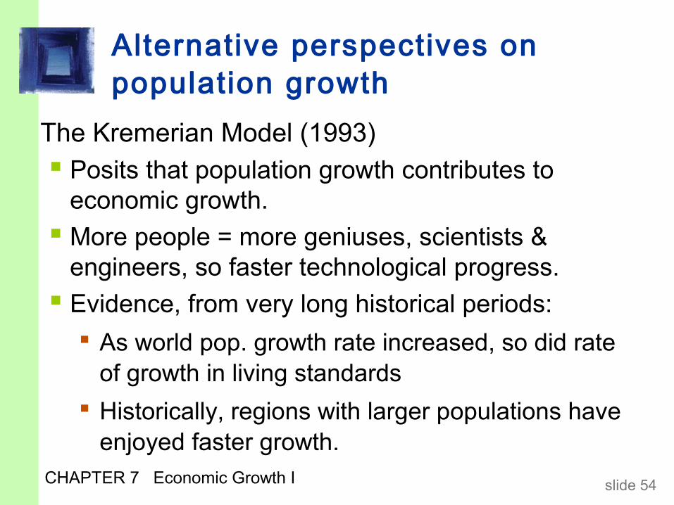
Alternative perspectives on population growth
The Kremerian Model (1993) Posits that population growth contributes to
economic growth.
More people = more geniuses, scientists & engineers, so faster technological progress.
Evidence, from very long historical periods:
As world pop. growth rate increased, so did rate of growth in living standards
Historically, regions with larger populations have enjoyed faster growth.
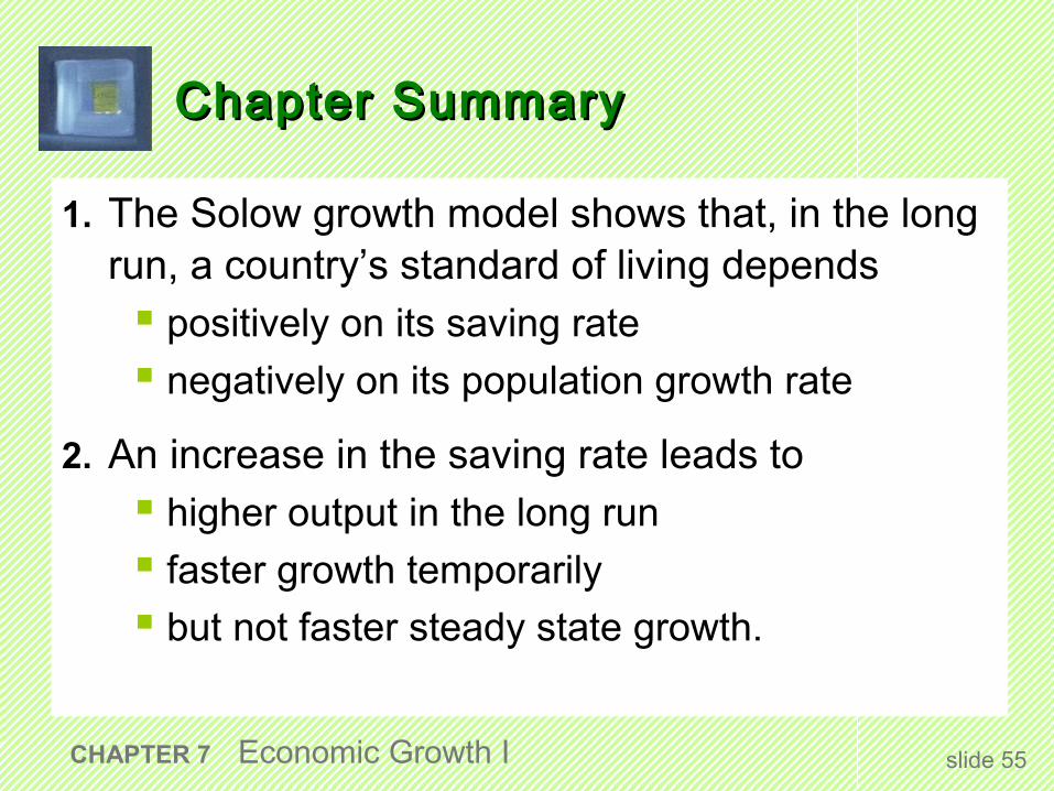
Chapter SummaryChapter Summary
1. The Solow growth model shows that, in the long run, a country’s standard of living depends positively on its saving rate
negatively on its population growth rate
2. An increase in the saving rate leads to higher output in the long run
faster growth temporarily
but not faster steady state growth.
CHAPTER 7 Economic Growth I slide 55
Chapter SummaryChapter Summary
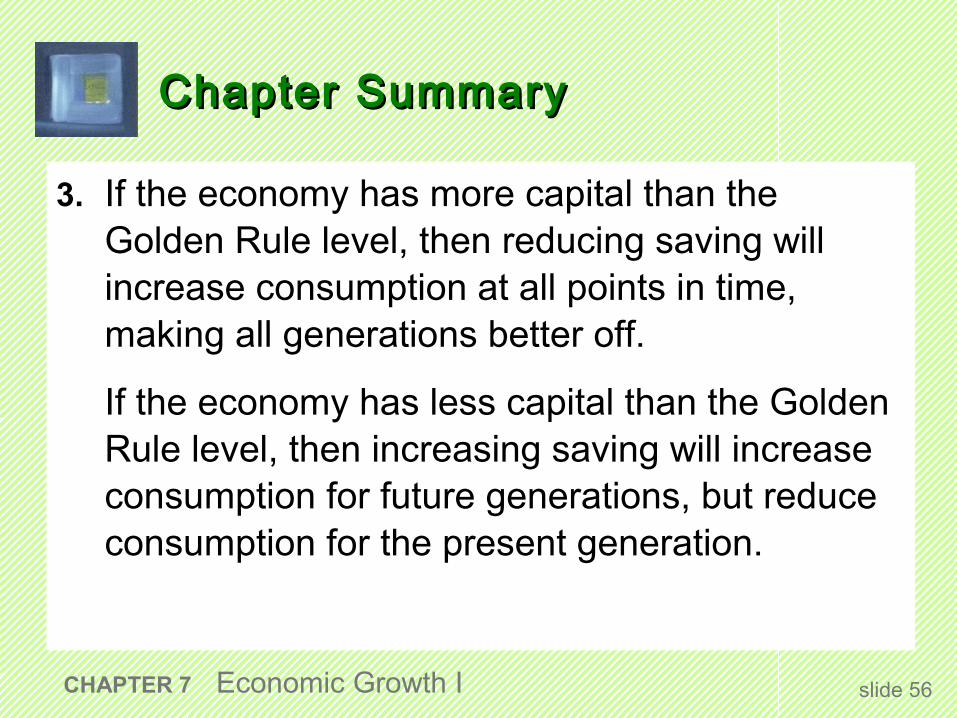
3. If the economy has more capital than the Golden Rule level, then reducing saving will increase consumption at all points in time, making all generations better off.
If the economy has less capital than the Golden Rule level, then increasing saving will increase consumption for future generations, but reduce consumption for the present generation.
CHAPTER 7 Economic Growth I slide 56