Embed Size (px)
Citation preview

Markov Chain Monte Carlo (MCMC) for model and parameter identification N. Pedroni, [email protected]
Multidisciplinary Course: Monte Carlo Simulation Methods for the Quantitative Analysis of Stochastic and Uncertain Systems
Nicola Pedroni
2Problem statement: statistical inference
Real systemSystem model
(parameters)
{ }nθθθ ...,,, 21=θExperimental data
{ }Nxxx ...,,, 21=x
(e.g., a mechanical
component)
(e.g., failure times)
(e.g., failure rate)
On the basis of the experimental data x, estimate the (unknown) parameters θof the (known) model
θ̂
(e.g., Exponential)
Nicola Pedroni
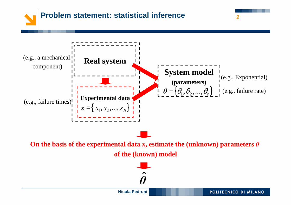
3Statistical inference – Example: component with constant failure rate
Exponential distribution
t
f(t) ( ) tt eetf θλ θλ −− ==
x = {x1, x2, …, xN}= t = { t1, t2, …, tN} = {1.71h, 48.8h, …, 0.39h}
(N = 100 failure times from N = 100 ‘identical’ components)
MODEL PARAMETER θ? (= FAILURE RATE λ?)
SYSTEM MODEL (hypothesis)
EXPERIMENTAL DATA (from real components)
Component failure time
Nicola Pedroni
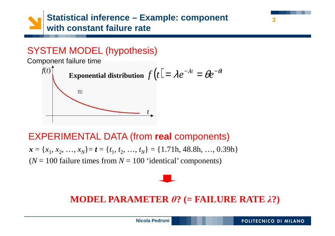
4Statistical inference: classical (frequentist) approach
•Only the (random) data are used to estimate the parameter
(e.g.) MAXIMUM LIKELIHOOD ESTIMATION
1-23
1
h1028.3h1005.3
100
timeobservedTotal
failurescollectedofNumber
time
failuresˆˆ −
=
⋅=⋅
===
==∑N
iit
Nλθ
x = {x1, x2, …, xN}= t = { t1, t2, …, tN} (N = 100 failure times)
(NB: also confidence intervals can be computed, reflecting the variability in the random data)
Nicola Pedroni
5Statistical inference: the Bayesian approach
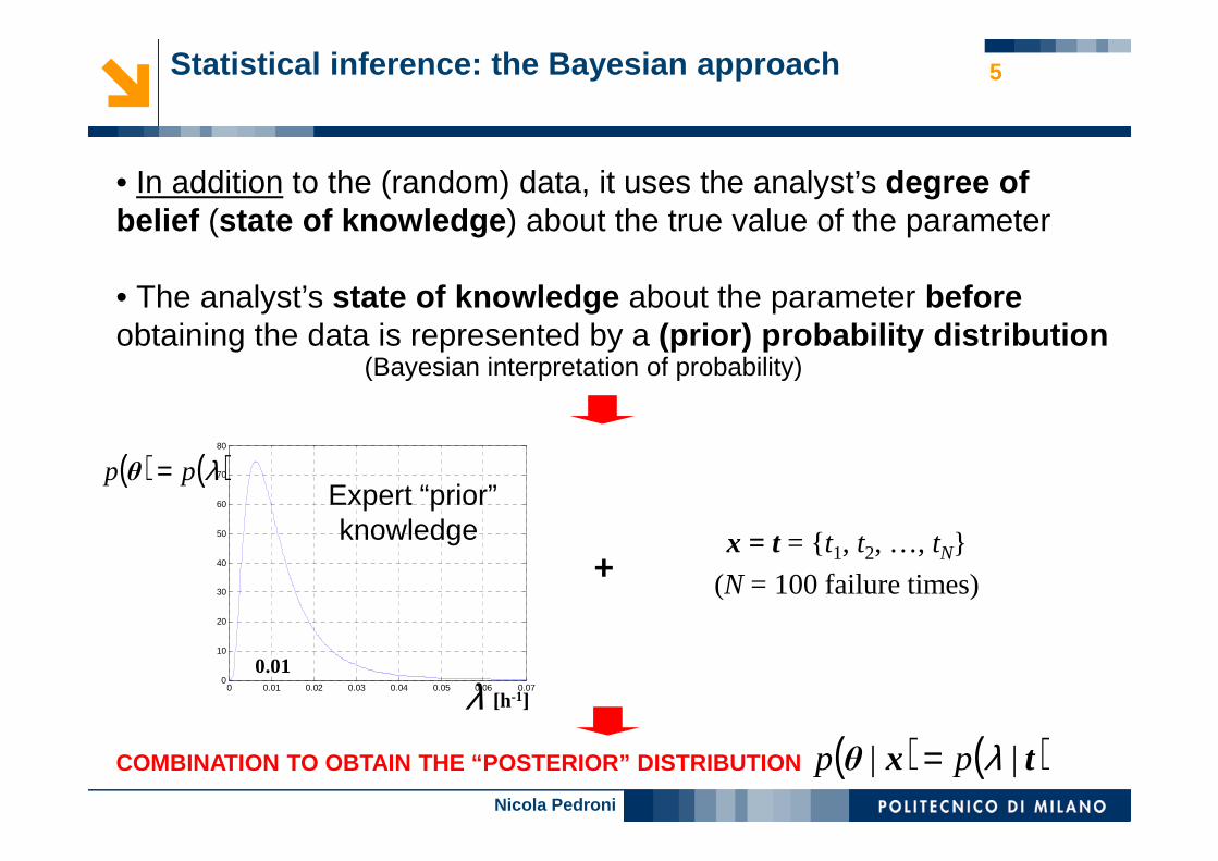
• In addition to the (random) data, it uses the analyst’s degree of belief (state of knowledge ) about the true value of the parameter
• The analyst’s state of knowledge about the parameter beforeobtaining the data is represented by a (prior) probability distribution
(Bayesian interpretation of probability)
x = t = { t1, t2, …, tN}
(N = 100 failure times)+
0 0.01 0.02 0.03 0.04 0.05 0.06 0.070
10
20
30
40
50
60
70
80
0.01
[h-1]
Expert “prior”knowledge
( ) ( )λpp =θ
COMBINATION TO OBTAIN THE “POSTERIOR” DISTRIBUTION ( ) ( )txθ || λpp =
λ
Nicola Pedroni
6Bayesian statistical inference: definitions
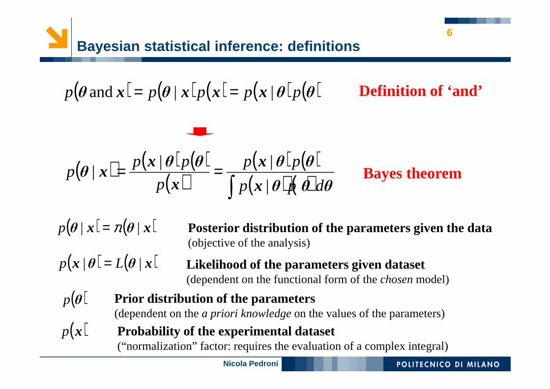
Bayes theorem( ) ( ) ( )( )
( ) ( )( ) ( )∫
==θθθx
θθxxθθx
xθdpp
pp
p
ppp
|
|||
( ) ( )xθθx || Lp = Likelihood of the parameters given dataset(dependent on the functional form of the chosenmodel)
( )θp Prior distribution of the parameters(dependent on the a priori knowledgeon the values of the parameters)
( )xp Probability of the experimental dataset(“normalization” factor: requires the evaluation of a complex integral)
( ) ( )xθxθ || π=p Posterior distribution of the parameters given the data(objective of the analysis)
Definition of ‘and’ ( ) ( ) ( ) ( ) ( )θθxxxθxθ ppppp ||and ==
Nicola Pedroni
7Bayesian statistical inference – Example: component with constant failure rate
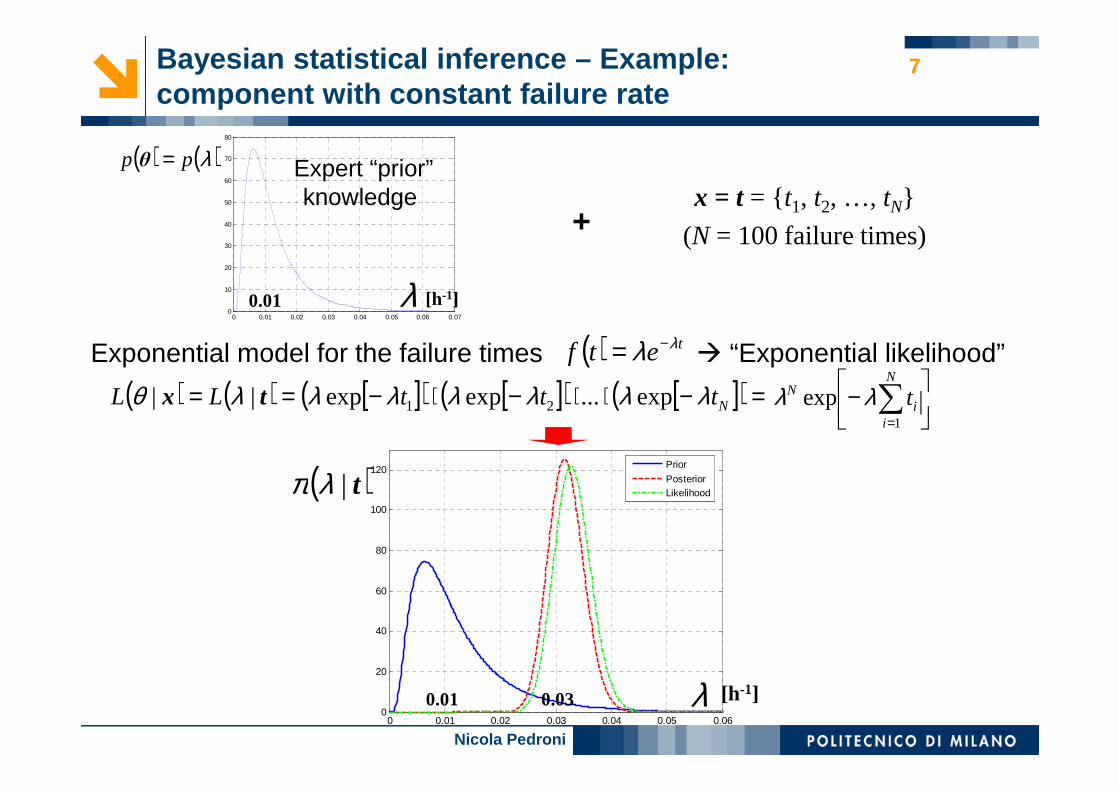
Exponential model for the failure times � “Exponential likelihood”
x = t = { t1, t2, …, tN}
(N = 100 failure times)+
0 0.01 0.02 0.03 0.04 0.05 0.06 0.070
10
20
30
40
50
60
70
80
0.01 [h-1]
Expert “prior”knowledge
( ) ( )λpp =θ
λ
− ∑=
N
ii
N t1
exp λλ( ) ( ) [ ]( ) [ ]( ) [ ]( ) =−⋅⋅−⋅−== NtttLL λλλλλλλθ exp...expexp|| 21tx
0 0.01 0.02 0.03 0.04 0.05 0.060
20
40
60
80
100
120 Prior
PosteriorLikelihood
0.01 0.03 [h-1]λ
( )t|λπ
( ) tetf λλ −=
Nicola Pedroni
8Bayesian statistical inference: Markov Chain Monte Carlo (MCMC) simulation approach
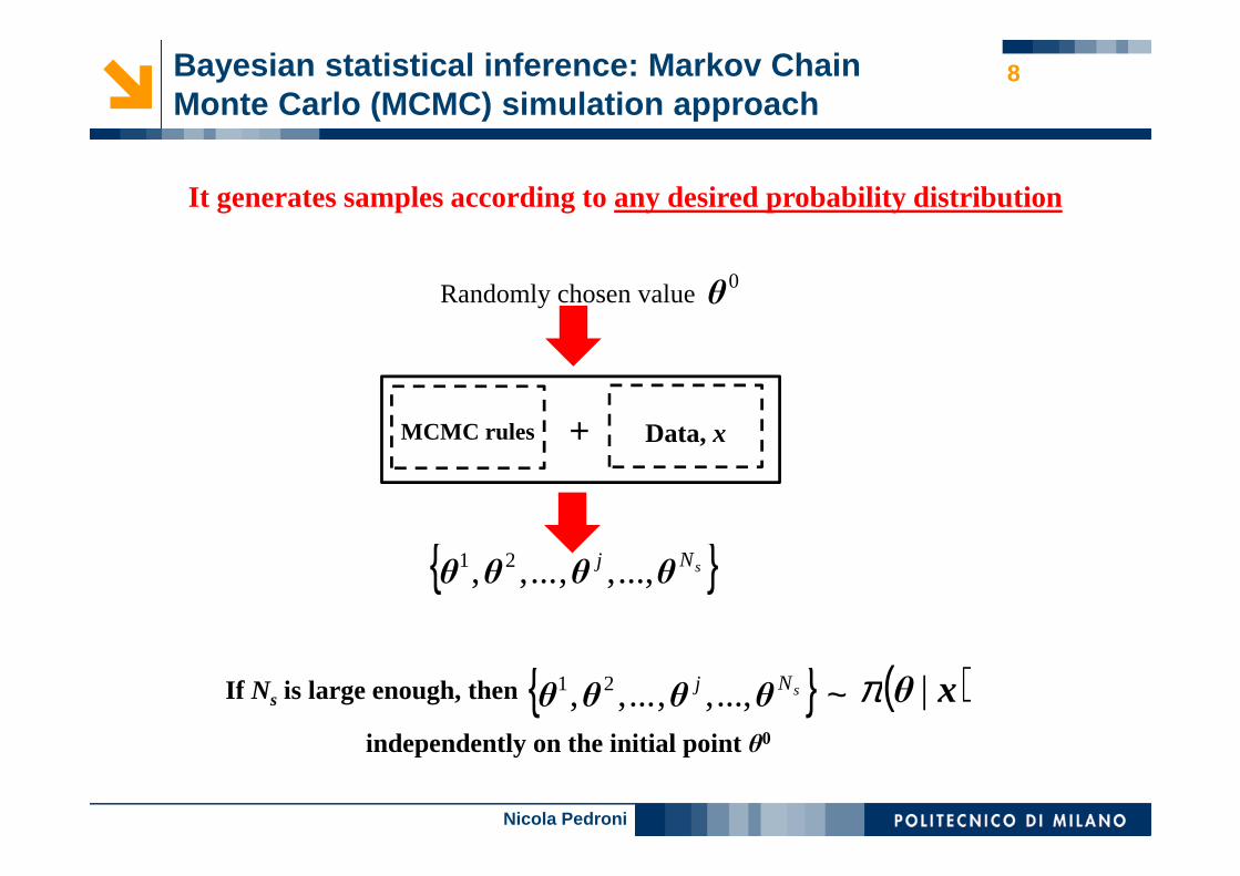
It generates samples according to any desired probability distribution
0θRandomly chosen value
MCMC rules Data, x+
{ }sNjθθθθ ...,,,...,, 21 ~ ( )xθ |πIf Ns is large enough, then
{ }sNjθθθθ ...,,,...,, 21
independently on the initial point θ0
Nicola Pedroni
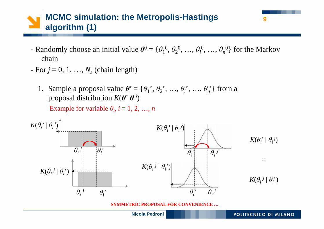
9MCMC simulation: the Metropolis-Hastings algorithm (1)
- Randomly choose an initial value θ0 = {θ10, θ2
0, …, θi0, …, θn
0} for the Markov chain
- For j = 0, 1, …, Ns (chain length)
1. Sample a proposal value θ’ = { θ1’, θ2’, …, θi’, …, θn'} from a proposal distribution K(θ’|θ j)
θij
K(θi’ | θi j)
=
K(θij | θi’)
θi'
SYMMETRIC PROPOSAL FOR CONVENIENCE …
Example for variable θi, i = 1, 2, …, n
θij θi'
θijθi'
θijθi'
K(θi’ | θi j)
K(θij | θi’)
K(θi’ | θi j)
K(θij | θi’)
Nicola Pedroni
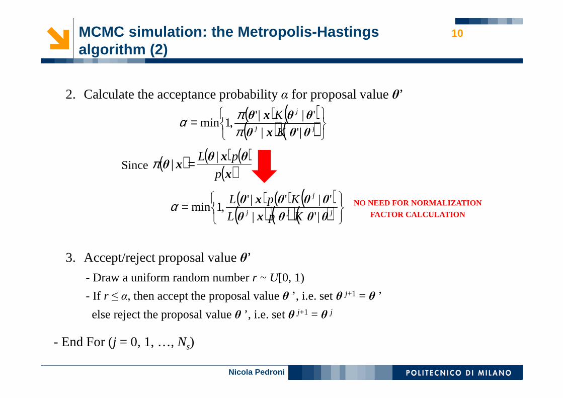
10MCMC simulation: the Metropolis-Hastings algorithm (2)
3. Accept/reject proposal value θ’
- Draw a uniform random number r ~ U[0, 1)
- If r ≤ α, then accept the proposal value θ ’, i.e. set θ j+1 = θ ’
else reject the proposal value θ ’, i.e. set θ j+1 = θ j
- End For (j = 0, 1, …, Ns)
2. Calculate the acceptance probability α for proposal value θ’
( ) ( )( ) ( )
=jj
j
K
K
θθxθ
θθxθ
|'|
'||',1minππα
Since ( ) ( ) ( )( )x
θxθxθ
p
pL || =π
( ) ( ) ( )( ) ( ) ( )
=jjj
j
KpL
KpL
θθθxθ
θθθxθ
|'|
'|'|',1minα NO NEED FOR NORMALIZATION
FACTOR CALCULATION

Nicola Pedroni
11
Application:component with constant failure rate
Nicola Pedroni
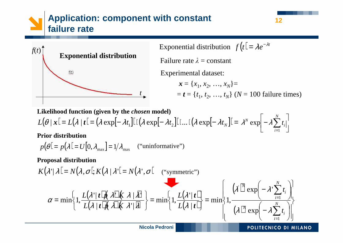
12Application: component with constant failure rate
Exponential distribution
t
f(t) ( ) tetf λλ −=Exponential distribution
Experimental dataset:
x = {x1, x2, …, xN}=
= t = { t1, t2, …, tN} (N = 100 failure times)
Failure rate λ = constant
Likelihood function (given by the chosen model)
− ∑=
N
ii
N t1
exp λλ( ) ( ) [ ]( ) [ ]( ) [ ]( ) =−⋅⋅−⋅−== NtttLL λλλλλλλθ exp...expexp|| 21tx
Prior distribution
( ) ( ) [ ] maxmax 1,0 λλλθ === Upp
Proposal distribution
( ) ( ) ( ) ( )σλλλσλλλ ,''|;,|' NKNK ==
( ) ( ) ( )( ) ( ) ( )
( )( )
( )
( )
−
−=
=
=
∑
∑
=
=N
ii
N
N
ii
N
t
t
L
L
KpL
KpL
1
1
'
exp
'exp
,1min|
|',1min
|'|
'|'|',1min
λλ
λλ
λλ
λλλλλλλλα
tt
tt
(“uninformative”)
(“symmetric”)

Nicola Pedroni
13Application: results
Posterior distribution Convergence of the chain
Burn-in period
GOOD AGREEMENT WITH “TRUE” VALUE, λ = 0.01

Nicola Pedroni
1414
The reversible-jump MCMC algorithm
Nicola Pedroni
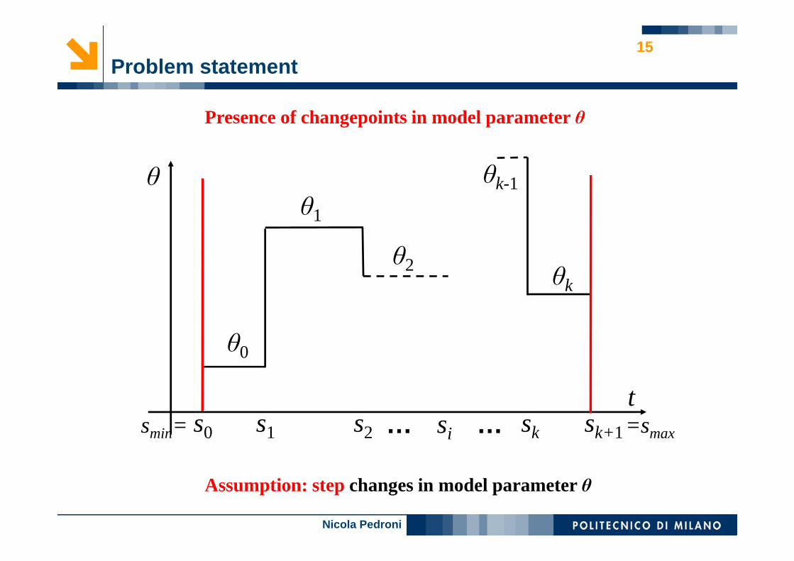
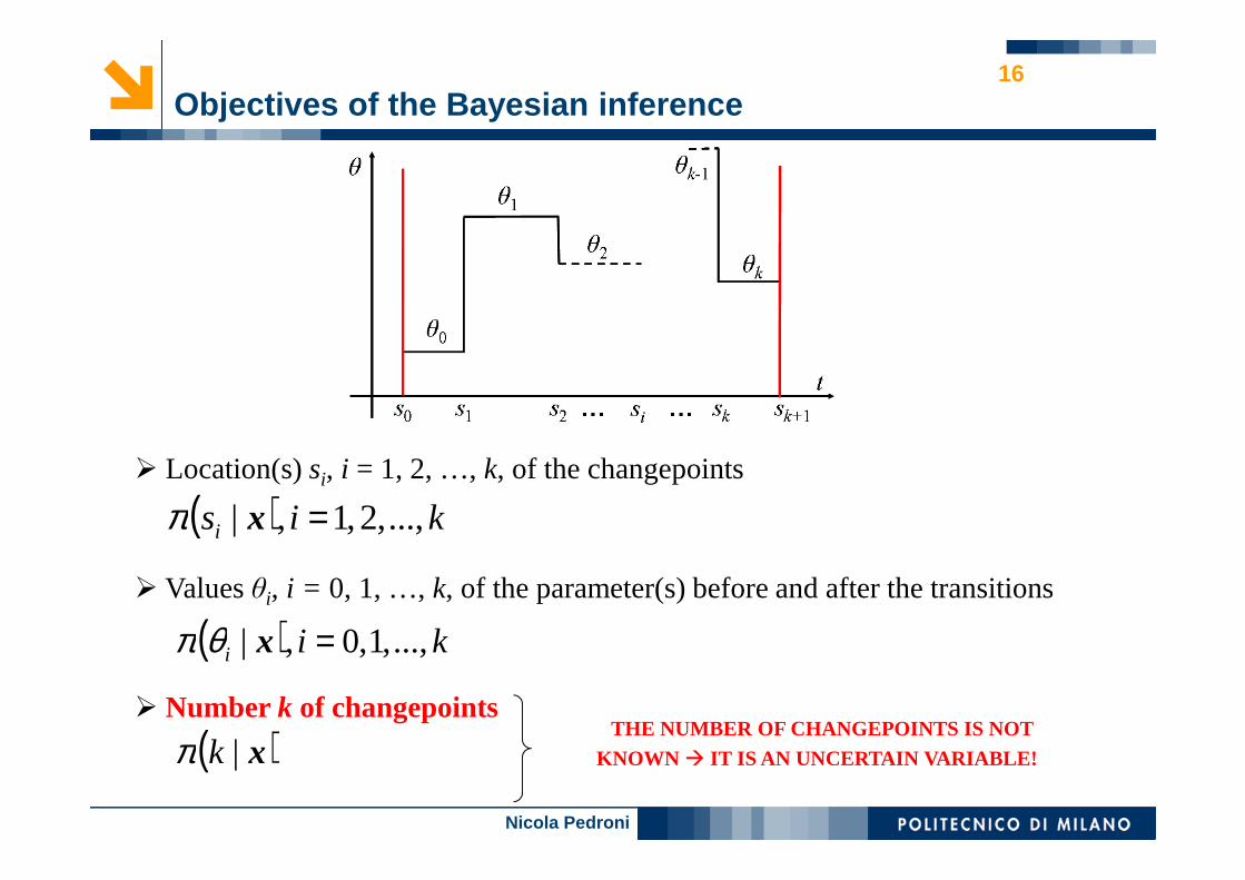
15Problem statement
Presence of changepoints in model parameter θ
Assumption: stepchanges in model parameter θ
θ
ts0 s1 s2 sk sk+1…
θ0
θ1
θ2
θk-1
θk
si …smin= =smax
Nicola Pedroni
16Objectives of the Bayesian inference
� Location(s) si, i = 1, 2, …, k, of the changepoints
� Values θi, i = 0, 1, …, k, of the parameter(s) before and after the transitions
� Number k of changepoints
( ) kisi ...,,2,1,| =xπ
( ) kii ...,,1,0,| =xθπ
( )x|kπTHE NUMBER OF CHANGEPOINTS IS NOT
KNOWN � IT IS AN UNCERTAIN VARIABLE!
Nicola Pedroni
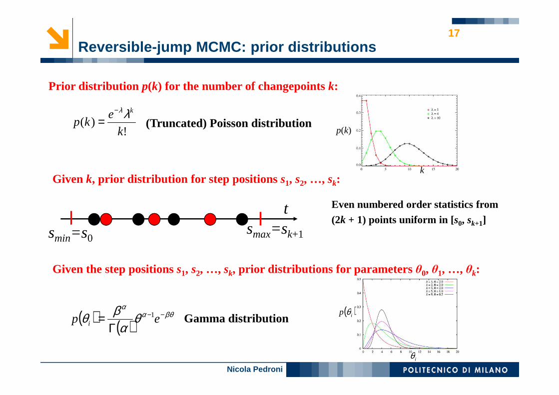
17Reversible-jump MCMC: prior distributions
Prior distribution p(k) for the number of changepoints k:
!)(
k
ekp
kλλ−
= (Truncated) Poisson distribution
k
p(k)
Given the step positions s1, s2, …, sk, prior distributions for parameters θ0, θ1, …, θk:
( ) ( )βθα
α
θα
βθ −−
Γ= ep i
1 Gamma distribution( )ip θ
iθ
Given k, prior distribution for step positions s1, s2, …, sk:
Even numbered order statistics from
(2k + 1) points uniform in [s0, sk+1]t
smin=s0smax=sk+1
Nicola Pedroni
18Reversible-jump MCMC: possible random moves
1. The parameter value θ is varied at a random location si
2. A randomly chosen step location si is moved
3. A new step location is created at random in the interval [s0, sk+1] (birth move)
4. A randomly chosen location si is eliminated (death move)
Four possible random moves to explore the uncertain parameter space:
Nicola Pedroni
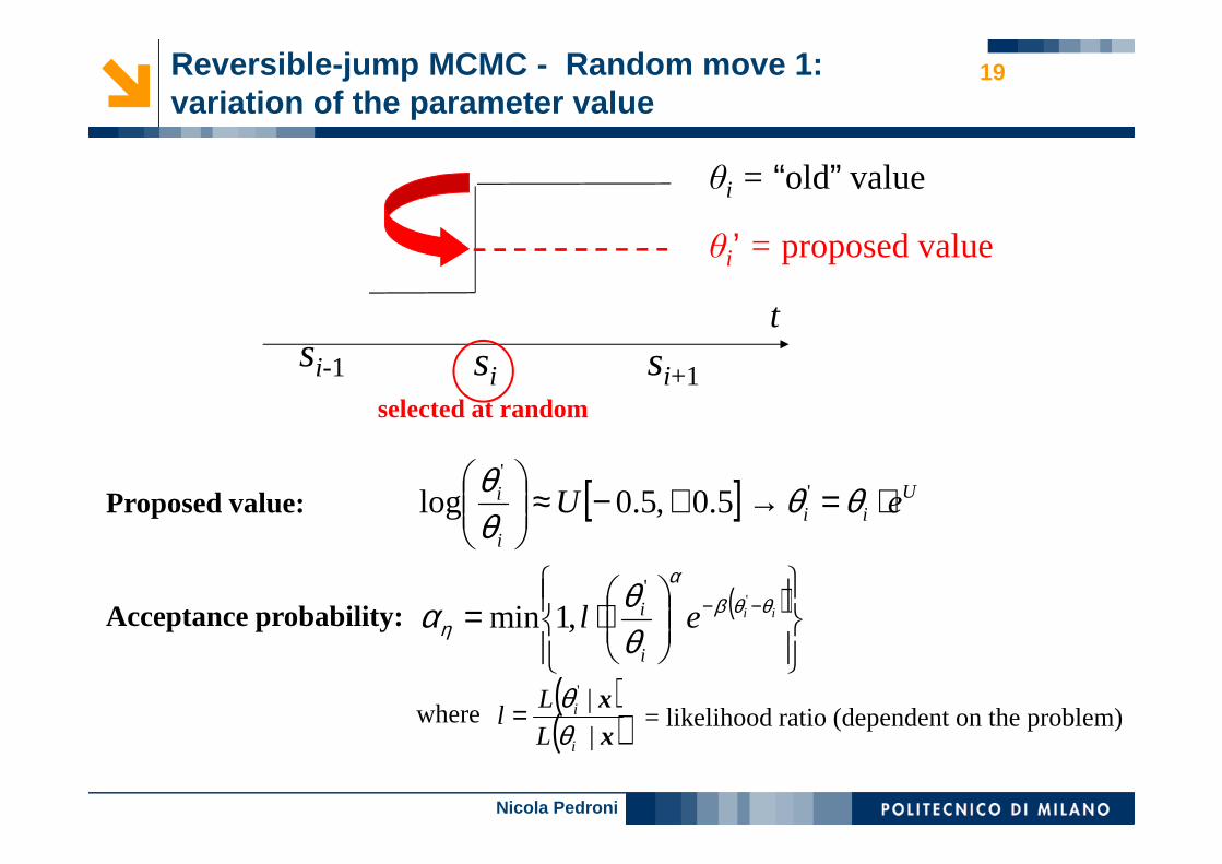
19Reversible-jump MCMC - Random move 1: variation of the parameter value
sisi-1 si+1
t
selected at random
θi = “old” value
θi’ = proposed value
[ ] Uii
i
i eU ⋅=→+−≈
θθ
θθ '
'
5.0,5.0logProposed value:
Acceptance probability: ( )
⋅= −− iiel
i
i θθβα
η θθα
''
,1min
where( )( )x
x|
|'
i
i
L
Ll
θθ= = likelihood ratio (dependent on the problem)
Nicola Pedroni
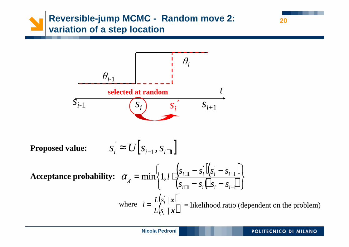
20Reversible-jump MCMC - Random move 2: variation of a step location
sisi-1 si+1
tselected at random
si’
[ ]11' , +−≈ iii ssUsProposed value:
Acceptance probability:( )( )( )( )
−−−−⋅=
−+
−+
11
1''
1,1miniiii
iiii
ssss
sssslχα
where( )( )x
x|
|'
i
i
sL
sLl = = likelihood ratio (dependent on the problem)
θi-1
θi
Nicola Pedroni
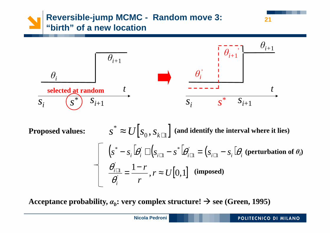
21Reversible-jump MCMC - Random move 3: “birth” of a new location
sisi+1
tselected at random
s* sisi+1
t
s*
θi
θi+ 1
θi+ 1
θi’
θi+ 1’
Proposed values: [ ]10* , +≈ kssUs (and identify the interval where it lies)
[ ]1,0,1
'
'1 Ur
r
r
i
i ≈−=+
θθ (imposed)
( ) ( ) ( ) iiiiiii ssssss θθθ −=−+− +++ 1'
1*
1'* (perturbation of θi)
Acceptance probability, αb: very complex structure! � see (Green, 1995)
Nicola Pedroni
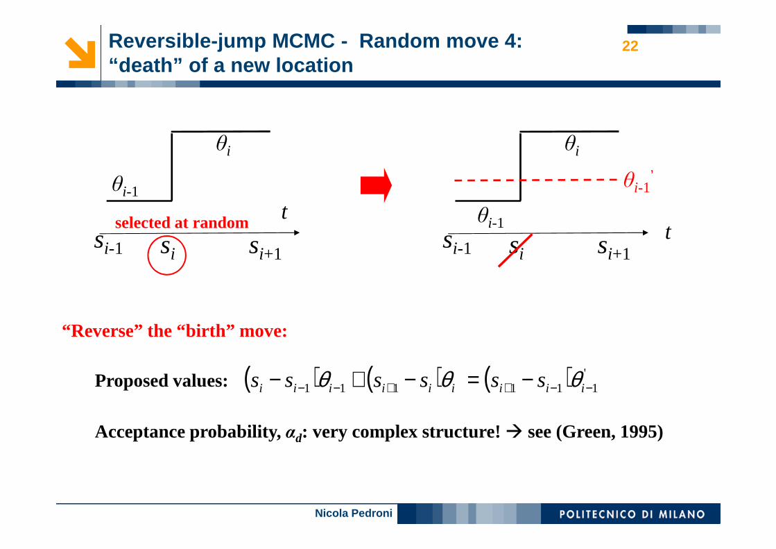
22Reversible-jump MCMC - Random move 4: “death” of a new location
sisi-1 si+1
tselected at random
θi-1
θi
sisi-1 si+1
tθi-1
θi
θi-1’
Proposed values: ( ) ( ) ( ) '111111 −−++−− −=−+− iiiiiiiii ssssss θθθ
Acceptance probability, αd: very complex structure! � see (Green, 1995)
“Reverse” the “birth” move:
Nicola Pedroni
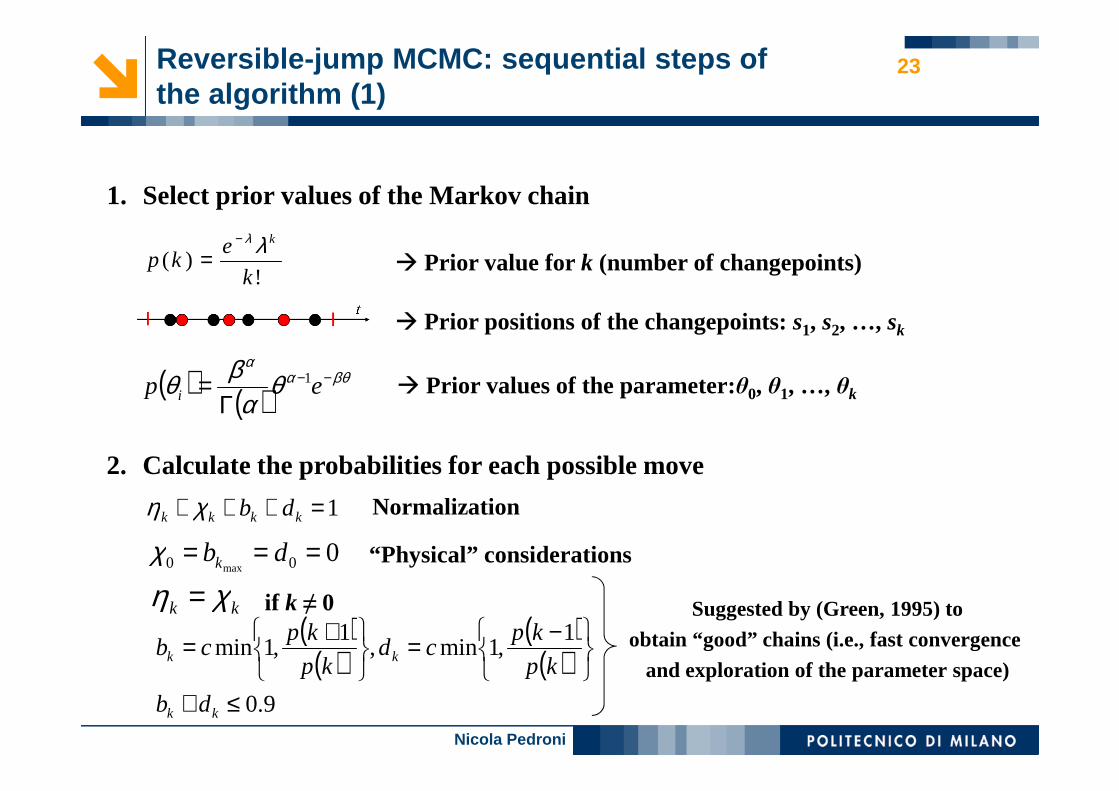
23Reversible-jump MCMC: sequential steps of the algorithm (1)
1. Select prior values of the Markov chain
!)(
k
ekp
kλλ−
= � Prior value for k (number of changepoints)
� Prior positions of the changepoints: s1, s2, …, sk
( ) ( )βθα
α
θα
βθ −−
Γ= ep i
1� Prior values of the parameter:θ0, θ1, …, θk
2. Calculate the probabilities for each possible move
1=+++ kkkk dbχη Normalization
000 max=== dbkχ “Physical” considerations
kk χη = Suggested by (Green, 1995) to
obtain “good” chains (i.e., fast convergence
and exploration of the parameter space)
( )( )
( )( )
9.0
1,1min,
1,1min
≤+
−=
+=
kk
kk
db
kp
kpcd
kp
kpcb
if k ≠ 0
Nicola Pedroni
24Reversible-jump MCMC: sequential steps of the algorithm (2)
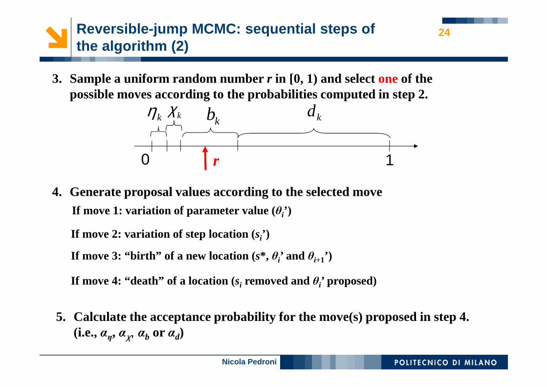
3. Sample a uniform random number r in [0, 1) and select oneof the possible moves according to the probabilities computed in step 2.
4. Generate proposal values according to the selected moveIf move 1: variation of parameter value (θi’)
If move 2: variation of step location (si’)
If move 3: “birth” of a new location (s*, θi’ and θi+1’)
If move 4: “death” of a location (si removed and θi’ proposed)
5. Calculate the acceptance probability for the move(s) proposed in step 4. (i.e., αη, αχ, αb or αd)
0 1
kηkb kd
r
kχ
Nicola Pedroni
25Reversible-jump MCMC: sequential steps of the algorithm (3)
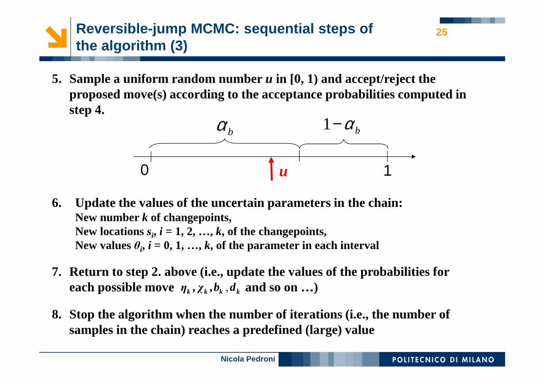
5. Sample a uniform random number u in [0, 1) and accept/reject the proposed move(s) according to the acceptance probabilities computed in step 4.
6. Update the values of the uncertain parameters in the chain: New number k of changepoints, New locations si, i = 1, 2, …, k, of the changepoints, New values θi, i = 0, 1, …, k, of the parameter in each interval
7. Return to step 2. above (i.e., update the values of the probabilities for each possible move and so on …)kkkk db,χ,η ,
8. Stop the algorithm when the number of iterations (i.e., the number of samples in the chain) reaches a predefined (large) value
0 1
bα bα−1
u
Nicola Pedroni
26Reversible-jump MCMC: example (1)
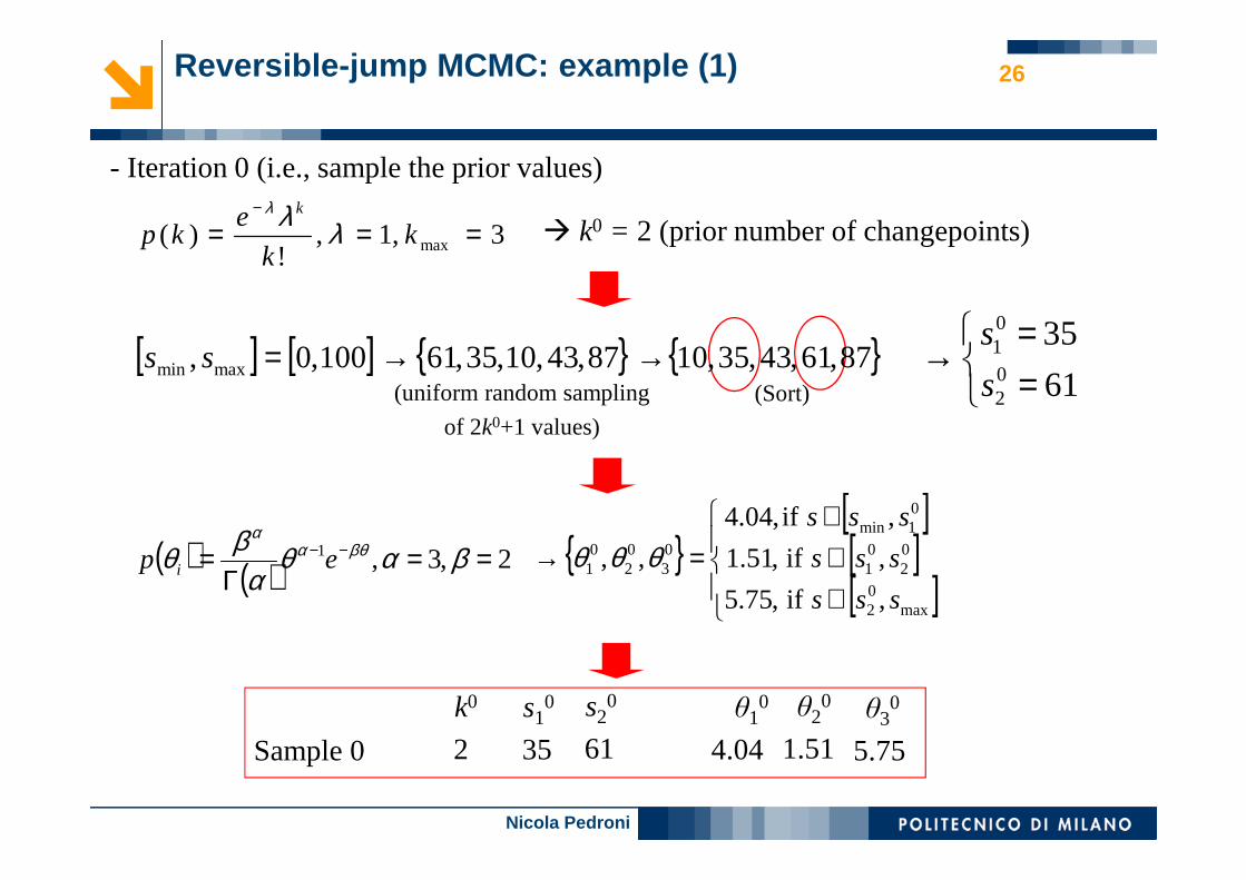
- Iteration 0 (i.e., sample the prior values)
3,1,!
)( max ===−
kk
ekp
k
λλλ� k0 = 2 (prior number of changepoints)
==
→61
3502
01
s
s
{ }[ ][ ][ ]
∈∈∈
=→
max02
02
01
01min
03
02
01
,if,75.5
,if,51.1
,if,04.4
,,
sss
sss
sss
θθθ
Sample 0
k0 s10 s2
0 θ10 θ2
0 θ30
2 35 61 4.04 1.51 5.75
( ) ( ) 2,3,1 ==Γ
= −− βαθα
βθ βθαα
ep i
(Sort)
[ ] [ ] { } { }87,61,43,35,1087,43,10,35,61100,0, maxmin →→=ss(uniform random sampling
of 2k0+1 values)
Nicola Pedroni
27Reversible-jump MCMC: example (2)
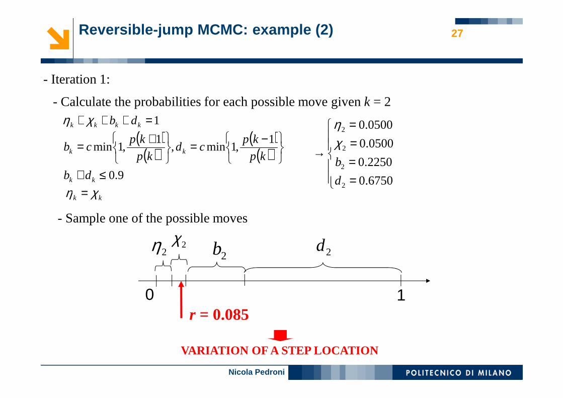
- Calculate the probabilities for each possible move given k = 21=+++ kkkk dbχη
kk χη =
( )( )
( )( )
9.0
1,1min,
1,1min
≤+
−=
+=
kk
kk
db
kp
kpcd
kp
kpcb
====
→
6750.0
2250.0
0500.0
0500.0
2
2
2
2
d
b
χη
- Sample one of the possible moves
0 1
2η 2χ2b 2d
r = 0.085
VARIATION OF A STEP LOCATION
- Iteration 1:
Nicola Pedroni
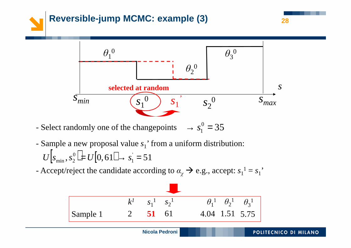
28Reversible-jump MCMC: example (3)
s10smin s2
0
sselected at random
s1’
θ10
θ20
smax
θ30
- Select randomly one of the changepoints 3501 =→ s
- Sample a new proposal value s1’ from a uniform distribution:
[ ) [ ) 5161,0, '1
02min =→= sUssU
- Accept/reject the candidate according to αχ� e.g., accept: s11 = s1’
Sample 1
k1 s11 s2
1 θ11 θ2
1 θ31
2 51 61 4.04 1.51 5.75
Nicola Pedroni
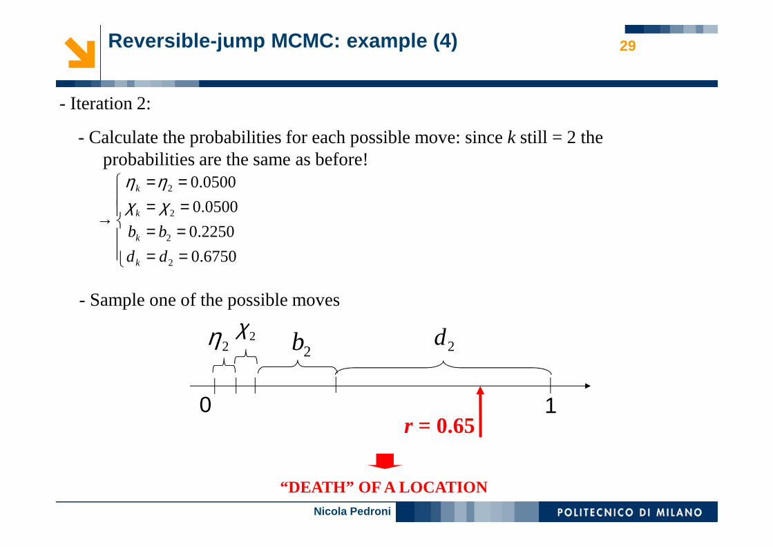
29Reversible-jump MCMC: example (4)
- Calculate the probabilities for each possible move: since k still = 2 the probabilities are the same as before!
========
→
6750.0
2250.0
0500.0
0500.0
2
2
2
2
dd
bb
k
k
k
k
χχηη
- Iteration 2:
- Sample one of the possible moves
0 1
2η 2χ2b 2d
r = 0.65
“DEATH” OF A LOCATION
Nicola Pedroni
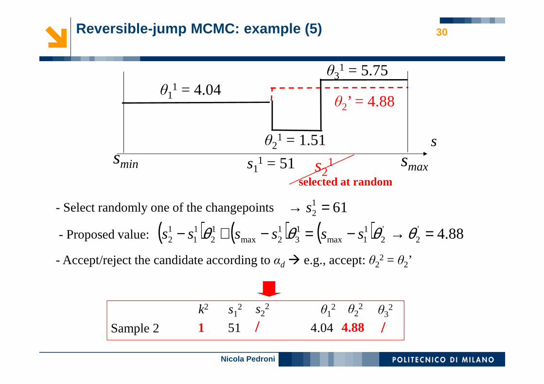
30Reversible-jump MCMC: example (5)
smin s21
s
selected at random
s11 = 51
θ11 = 4.04
θ21 = 1.51
smax
θ31 = 5.75
- Select randomly one of the changepoints 6112 =→ s
- Proposed value:( ) ( ) ( ) 88.4'2
'2
11max
13
12max
12
11
12 =→−=−+− θθθθ ssssss
θ2’ = 4.88
- Accept/reject the candidate according to αd � e.g., accept: θ22 = θ2’
Sample 2
k2 s12 s2
2 θ12 θ2
2 θ32
1 51 / 4.04 4.88 /
Nicola Pedroni
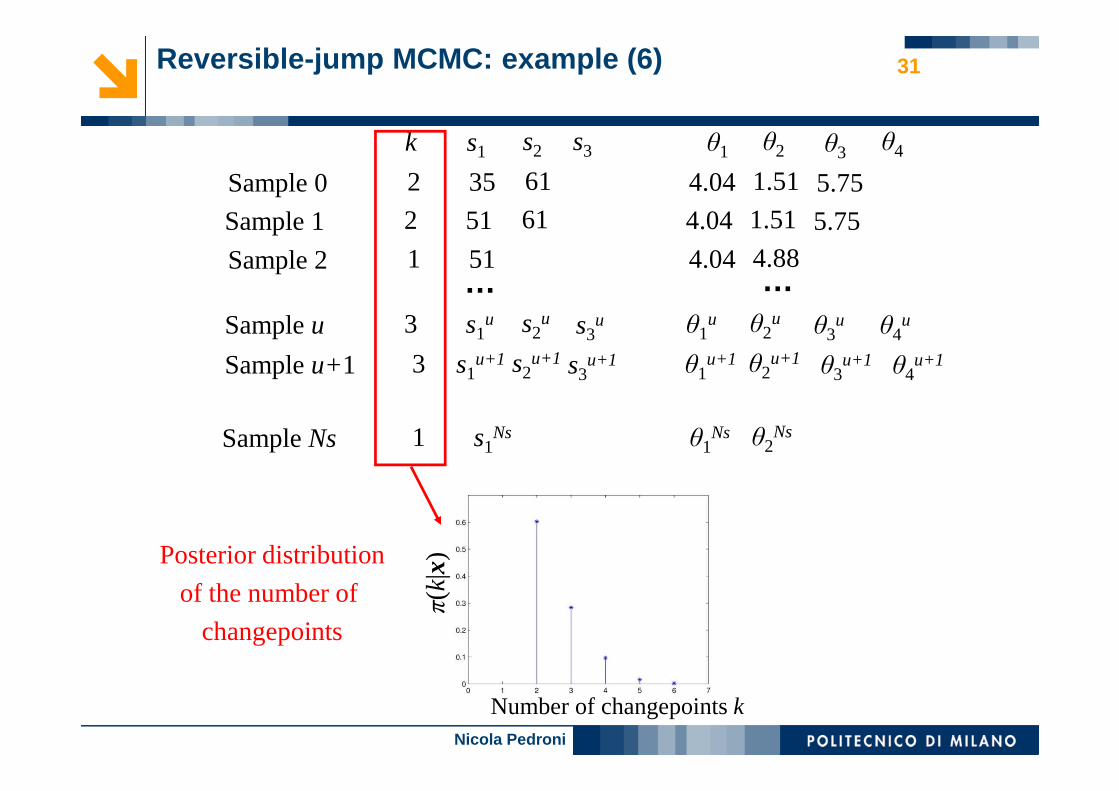
31Reversible-jump MCMC: example (6)
Sample 1
k s1 s2 θ1 θ2 θ3
2 51 61 4.04 1.51 5.75
Sample 0 2 35 61 4.04 1.51 5.75
Sample 2 1 51 4.04 4.88… …
Sample u 3 s1u s2
u θ1u θ2
u θ3u
s3
s3u
θ4
θ4u
Sample u+1 3 s1u+1 s2
u+1 θ1u+1 θ2
u+1 θ3u+1s3
u+1 θ4u+1
Sample Ns 1 s1Ns θ1
Ns θ2Ns
π(k
|x)
Number of changepoints k
Posterior distribution
of the number of
changepoints
Nicola Pedroni
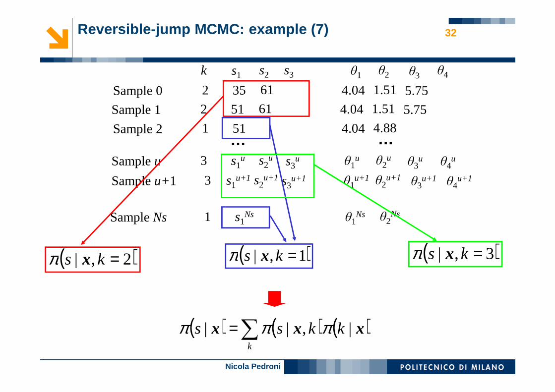
32Reversible-jump MCMC: example (7)
Sample 1
k s1 s2 θ1 θ2 θ3
2 51 61 4.04 1.51 5.75
Sample 0 2 35 61 4.04 1.51 5.75
Sample 2 1 51 4.04 4.88… …
Sample u 3 s1u s2
u θ1u θ2
u θ3u
s3
s3u
θ4
θ4u
Sample u+1 3 s1u+1 s2
u+1 θ1u+1 θ2
u+1 θ3u+1s3
u+1 θ4u+1
Sample Ns 1 s1Ns θ1
Ns θ2Ns
( )2,| =ks xπ ( )1,| =ks xπ ( )3,| =ks xπ
( ) ( ) ( )∑=k
kkss xxx |,|| πππ

Nicola Pedroni
33
Application 1:Component degradation
due to reparations or aging
Nicola Pedroni
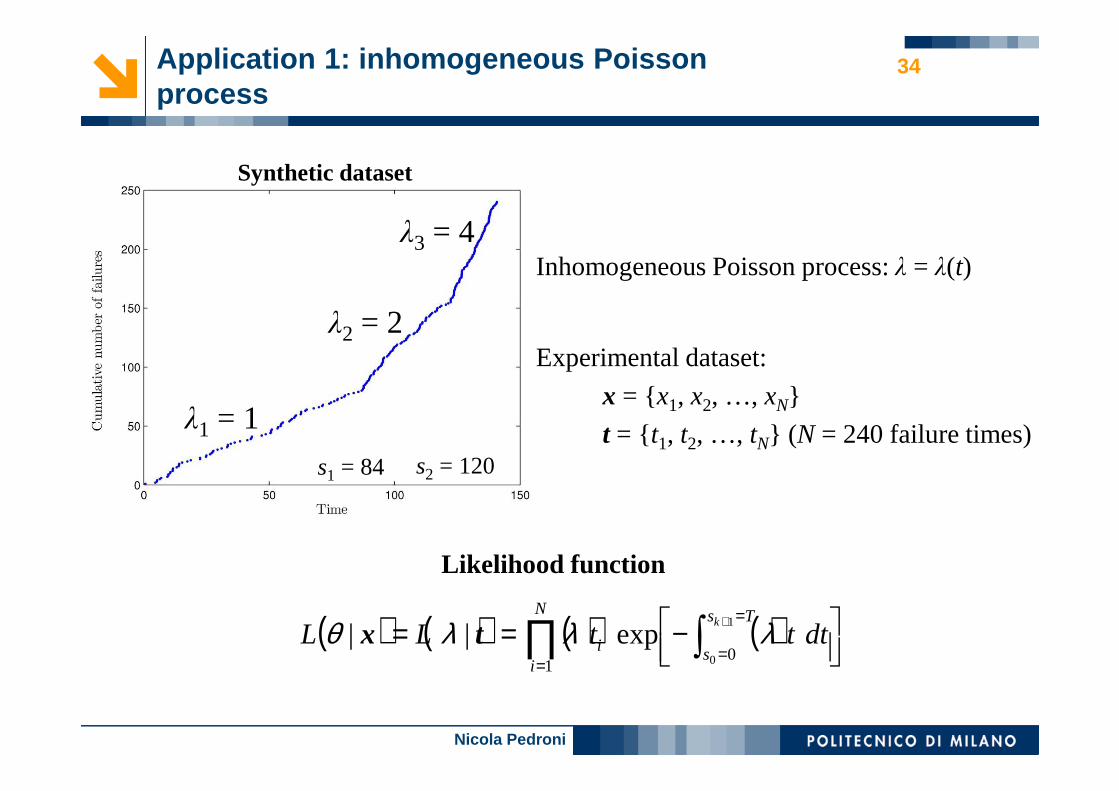
34Application 1: inhomogeneous Poisson process
Synthetic dataset
λ1 = 1
λ2 = 2
λ3 = 4
s1 = 84 s2 = 120
Inhomogeneous Poisson process: λ = λ(t)
Experimental dataset:
x = {x1, x2, …, xN}
t = { t1, t2, …, tN} (N = 240 failure times)
Likelihood function
( ) ( ) ( ) ( )
−== ∫∏
=
==
+ Ts
s
N
ii
k
dtttLL1
0 01
exp|| λλλθ tx
Nicola Pedroni
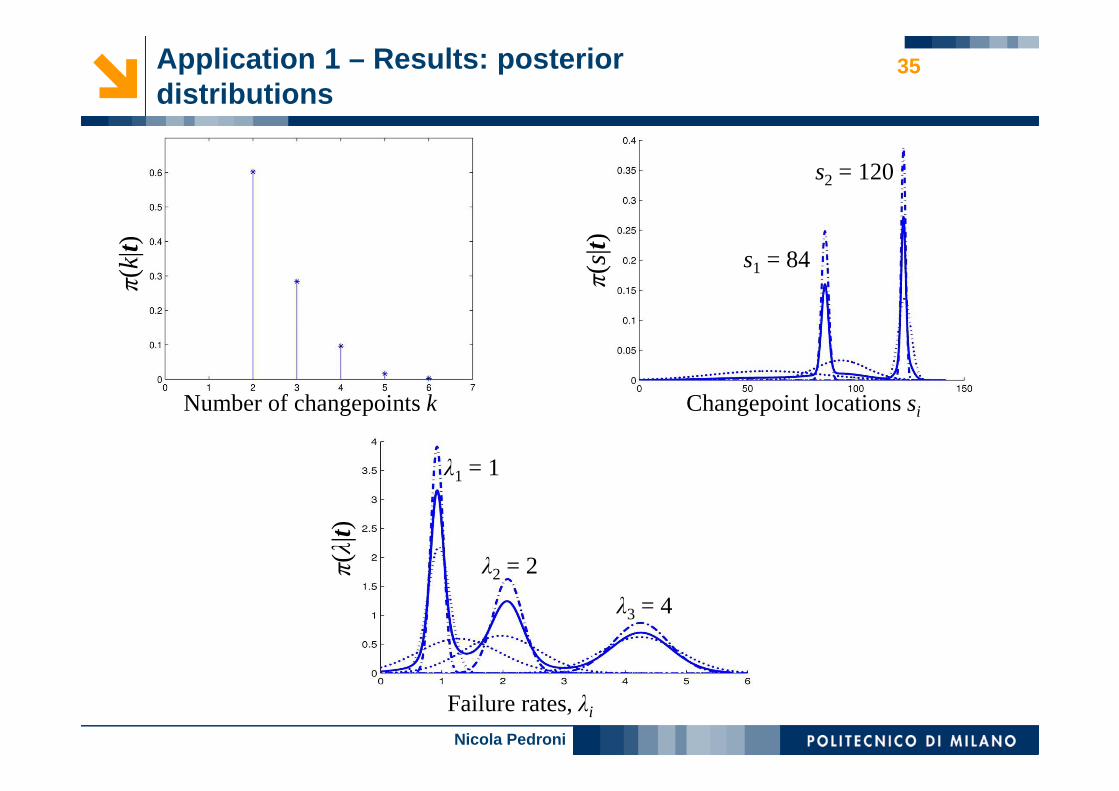
35Application 1 – Results: posterior distributions
π(k
|t)
Number of changepoints k Changepoint locations si
π(s
|t)
Failure rates, λi
π(λ
|t)
λ1 = 1
λ2 = 2
λ3 = 4
s1 = 84
s2 = 120

Nicola Pedroni
36
Application 2:Deterioration due to fatigue
Nicola Pedroni
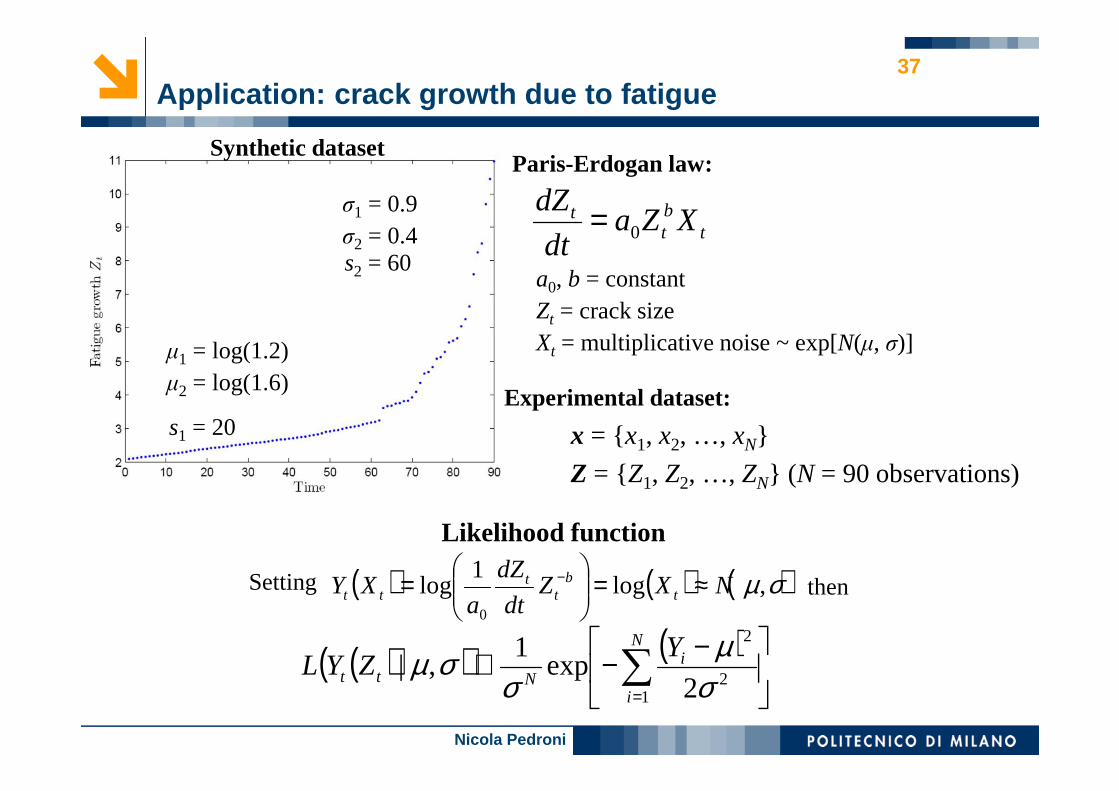
37Application: crack growth due to fatigue
Synthetic datasetParis-Erdogan law:
tbt
t XZadt
dZ0=
a0, b = constantZt = crack sizeXt = multiplicative noise ~ exp[N(µ, σ)]
Experimental dataset:
x = {x1, x2, …, xN}
Z = {Z1, Z2, …, ZN} (N = 90 observations)
s1 = 20
s2 = 60
µ1 = log(1.2)µ2 = log(1.6)
σ1 = 0.9σ2 = 0.4
Likelihood function
( )( ) ( )
−−∝ ∑=
N
i
iNtt
YZYL
12
2
2exp
1,|
σµ
σσµ
Setting ( ) ( ) ( )σµ,log1
log0
NXZdt
dZ
aXY t
bt
ttt ≈=
= − then
Nicola Pedroni
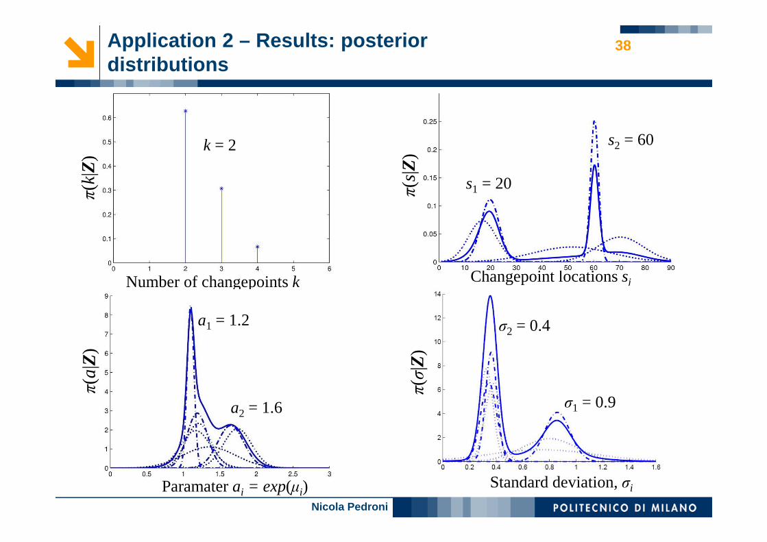
38Application 2 – Results: posterior distributions
π(k
|Z)
Number of changepoints k Changepoint locations si
π(s
|Z)
Standard deviation, σi
π(σ
|Z)
Paramater ai = exp(µi)
π(a
|Z)
a1 = 1.2
a2 = 1.6 σ1 = 0.9
s1 = 20
s2 = 60k = 2
σ2 = 0.4