Embed Size (px)
Citation preview

©B
eic
ip-F
ranla
b
232, Avenue Napoléon Bonaparte
P.O. BOX 213
92502 Rueil-Malmaison
France
Phone: +33 1 47 08 80 00
Fax: +33 1 47 08 41 85
www.beicip.com
Material Balance Calculations
The unfashionable tool
Victor Alcobia April 1st, 2014
©B
eic
ip-F
ranla
b
2
OBJECTIVES
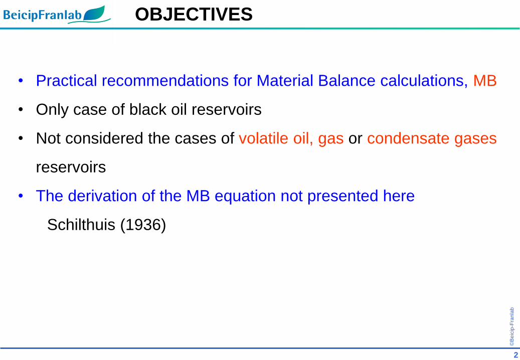
• Practical recommendations for Material Balance calculations, MB
• Only case of black oil reservoirs
• Not considered the cases of volatile oil, gas or condensate gases
reservoirs
• The derivation of the MB equation not presented here
Schilthuis (1936)

©B
eic
ip-F
ranla
b
3
Introduction
©B
eic
ip-F
ranla
b
4
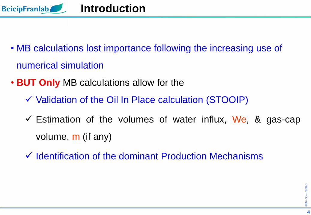
• MB calculations lost importance following the increasing use of
numerical simulation
• BUT Only MB calculations allow for the
Validation of the Oil In Place calculation (STOOIP)
Estimation of the volumes of water influx, We, & gas-cap
volume, m (if any)
Identification of the dominant Production Mechanisms
Introduction
©B
eic
ip-F
ranla
b
5
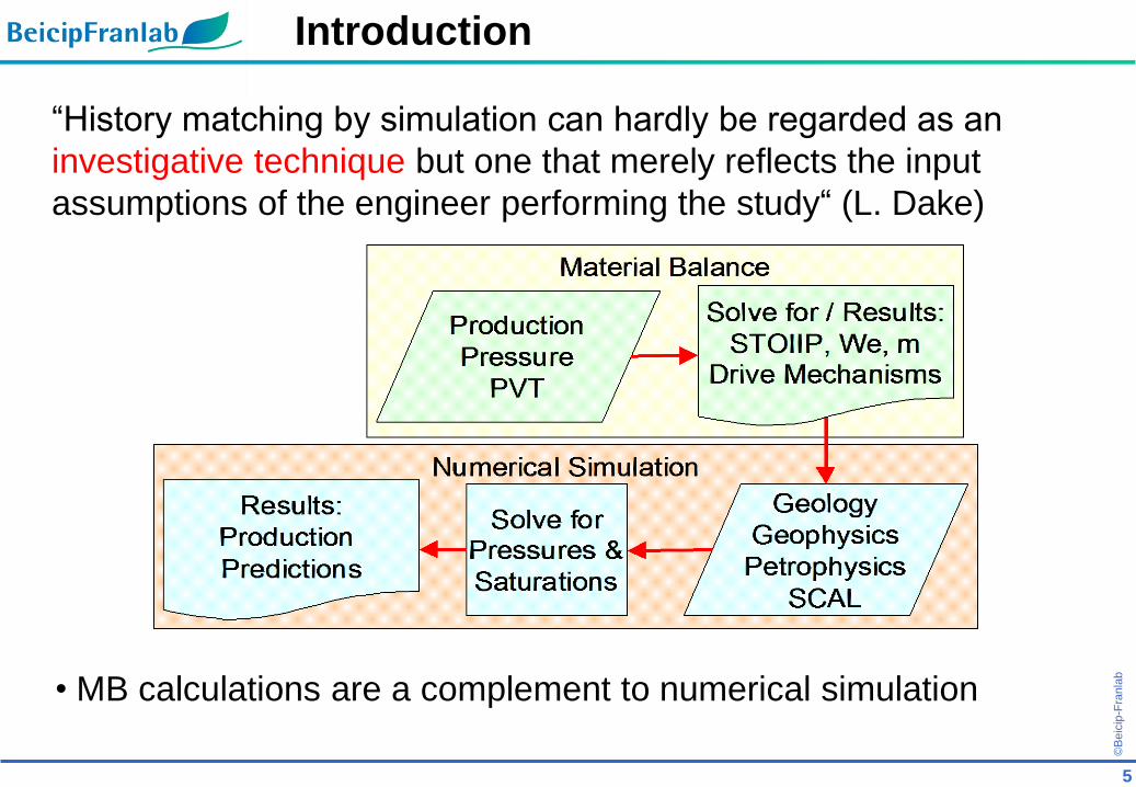
• MB calculations are a complement to numerical simulation
Introduction
“History matching by simulation can hardly be regarded as an
investigative technique but one that merely reflects the input
assumptions of the engineer performing the study“ (L. Dake)
©B
eic
ip-F
ranla
b
6
Introduction
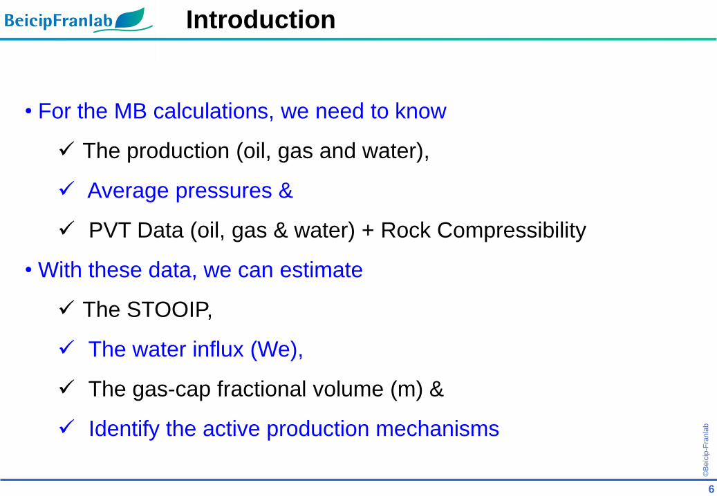
• For the MB calculations, we need to know
The production (oil, gas and water),
Average pressures &
PVT Data (oil, gas & water) + Rock Compressibility
• With these data, we can estimate
The STOOIP,
The water influx (We),
The gas-cap fractional volume (m) &
Identify the active production mechanisms
©B
eic
ip-F
ranla
b
7
Introduction
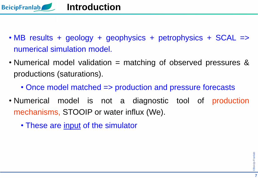
• MB results + geology + geophysics + petrophysics + SCAL =>
numerical simulation model.
• Numerical model validation = matching of observed pressures &
productions (saturations).
• Once model matched => production and pressure forecasts
• Numerical model is not a diagnostic tool of production
mechanisms, STOOIP or water influx (We).
• These are input of the simulator

©B
eic
ip-F
ranla
b
8
Material Balance Equation
©B
eic
ip-F
ranla
b
9
Basic Form MB Equation
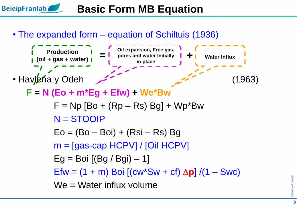
• The expanded form – equation of Schiltuis (1936)
Producción
(crudo + gas + agua) =Expansión de crudo,
gas libre, poros y aguaInicialmente en Sitio
+ Influjo de Agua
• Havlena y Odeh (1963)
F = N (Eo + m*Eg + Efw) + We*Bw
F = Np [Bo + (Rp – Rs) Bg] + Wp*Bw
N = STOOIP
Eo = (Bo – Boi) + (Rsi – Rs) Bg
m = [gas-cap HCPV] / [Oil HCPV]
Eg = Boi [(Bg / Bgi) – 1]
Efw = (1 + m) Boi [(cw*Sw + cf) p] /(1 – Swc)
We = Water influx volume
Production
(oil + gas + water)
Oil expansion, Free gas,
pores and water Initially
in place Water Influx

©B
eic
ip-F
ranla
b
10
• F represents the production at reservoir conditions,
• Sometimes Bt & Bti are used instead of Bo & Boi.
• Bt = Bo + Bg * (Rsi – Rs)
• Bti = Boi
• Eo => oil + solution gas expansion
• Eg => gas-cap expansion and
• Efw => Pores & interstitial water expansion
• Eo, Eg y Efw represent the drive indices.
Basic Form MB Equation
©B
eic
ip-F
ranla
b
11
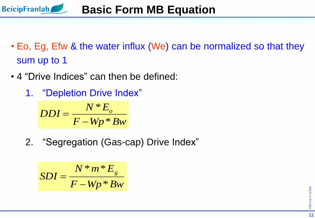
• Eo, Eg, Efw & the water influx (We) can be normalized so that they
sum up to 1
• 4 “Drive Indices” can then be defined:
1. “Depletion Drive Index”
2. “Segregation (Gas-cap) Drive Index”
BwWpF
ENDDI o
*
*
BwWpF
EmNSDI
g
*
**
Basic Form MB Equation

©B
eic
ip-F
ranla
b
12
• 4 “Drive Indices” then can be defined:
3. “Water Drive Index”
4. “Formation & Connate Water Drive Index”
DDI + SDI + WDI + CDI = 1
BwWpF
BwWpWWDI e
*
*
BwWpF
EmNCDI
fw
*
*)1(*
Basic Form MB Equation
©B
eic
ip-F
ranla
b
13
• MB equation is simplified if there is no active aquifer nor initial
gas-cap.
• Efw could be dismissed if there is a gas-cap but this hypothesis
must be verified => Significant errors.
• Gas or water injection (if any) must be deducted from the
produced volumes
• Pressure appears explicitly in the Efw index, but pressure is
required to estimate volumetric factors and water influx.
• Representing the MB equation as a straight line facilitates
the identification of the production mechanisms
• And allows for the calculation of unknown parameters as the
STOOIP or the water influx from an aquifer
Basic Form MB Equation

©B
eic
ip-F
ranla
b
14
Solution of the MB Equation
©B
eic
ip-F
ranla
b
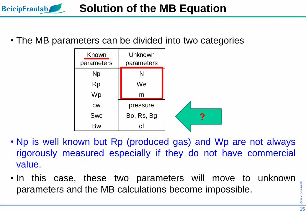
Known
parameters
Unknown
parameters
Np N
Rp We
Wp m
cw pressure
Swc Bo, Rs, Bg
Bw cf
15
• The MB parameters can be divided into two categories
Solution of the MB Equation
• Np is well known but Rp (produced gas) and Wp are not always
rigorously measured especially if they do not have commercial
value.
• In this case, these two parameters will move to unknown
parameters and the MB calculations become impossible.
?
©B
eic
ip-F
ranla
b
16
• The volumetric estimate of the STOOIP is a reference, but MB
estimates the “efective” STOOIP (drained by current wells).
• The STOOIP of an isolated block without any wells will never be
"seen" or detected by the MB.
• Parameter with greater uncertainty = influx of water, We. Can be
detected but its size is rarely known.
• Same for m (ratio of gas-cap to oil volumes).
Often however the presence of a gas-cap can be detected and
the gas-oil contact can be determined (with RFT/MDT, well
tests, electrical logs and PVT).
Solution of the MB Equation

©B
eic
ip-F
ranla
b
17
• Pressures are measured (flowing or closed wells) = known
parameters
• But the average pressures used in the calculations are estimated
in two steps,
Well test interpretation for each well to determine the average
pressure in the drainage area and the conversion of that
average pressure to the reservoir Datum.
Estimation of the reservoir (all wells) average pressure at the
Datum from the average pressures of each well
Solution of the MB Equation
©B
eic
ip-F
ranla
b
18
• The same can be applied to PVT properties (Bo, Rs y Bg) as a
result of a synthesis of several laboratory well tests at a Datum.
• Pore compressibility is often neglected (Schiltuis did it) but this can
lead to significant errors, particularly above bubble point pressure
with no free gas.
(Note: cf when pore pressure )
Solution of the MB Equation
©B
eic
ip-F
ranla
b
19
• There are two ways to "solve" the MB equation
1. Calculate pressures from production data + PVT + Assumed
Unknowns and compare them with the measured pressures
(iterative process. Better to use a spreadsheet)
2. Calculate the unknown parameter from the measured
pressures + production data + PVT and compare with the
appropriate Havlena & Odeh graphics shown later (LP Dake)
• There is no “conventional” solution for the MB equation,
considering the number of unknown parameters.
• All depends on the parameter(s) to be estimated (STOOIP, We, m,
cf or pressure).
Solution of the MB Equation

©B
eic
ip-F
ranla
b
20
Necessary conditions for MB
Application
©B
eic
ip-F
ranla
b
21
• There are no sufficient conditions to apply the MB equation but
there are two necessary conditions,
1. Existence of data (pressure, production and PVT) adequate in
terms of amount and quality
2. To be able to define an average pressure decline for the
reservoir.
• A reservoir with high hydraulic diffusivity (high k/c) presents
more uniform values of pressure. Low diffusivity implies greater
differences of pressure between wells.
• Different pressures in several regions do not prevent MB
calculations . But including isolated blocks with different pressure
“regimes” should not be done.
Necessary Conditions

©B
eic
ip-F
ranla
b
22
Data Validation and Calculation of
Averages
Production Data
©B
eic
ip-F
ranla
b
23
• Production data of oil, water and gas to be used are the Net
values = [Produced values – Injected values]
• Create graphics of productions and gas-oil and water-oil ratios to
detect anomalies.
• GOR and WOR tend to increase with time in each well, except if
coning occurs.
• Coning can be detected with some basic evaluations,
If the GOR or Water Cut depends on oil rate
If GOR or Water Cut decrease after a temporary shut in of the
well
Use of graphics of Chan (water “coning”).
Production Data
©B
eic
ip-F
ranla
b
24
• GOR tend to increase with time except when the wells more
affected by gas are shut.
• GOR cannot be larger than solution gas ratio if reservoir pressure
is above bubble point pressure.
• GOR cannot also be much lower than solution gas ratio.
• GOR reports can be wrong in cases of wells with artificial gas-lift.
Production Data

©B
eic
ip-F
ranla
b
25
Data Validation and Calculation of
Averages
Pressure Data
©B
eic
ip-F
ranla
b
26
• Steps for the calculation of Average Pressures in the reservoir:
Calculate average reservoir pressures in the drainage area of
each well
Convert these pressures to Datum depth
Calculate average reservoir pressures at Datum
• Reservoir pressures do not need to be uniform in all the reservoir
but all the wells must drain the same block (ensure pressure
communication)
Pressure Data
©B
eic
ip-F
ranla
b
Time
Pre
ssure
Time
Pre
ssure
(a) (b)
27
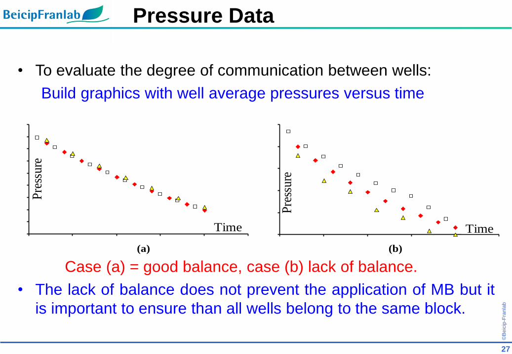
• To evaluate the degree of communication between wells:
Build graphics with well average pressures versus time
Case (a) = good balance, case (b) lack of balance.
• The lack of balance does not prevent the application of MB but it
is important to ensure than all wells belong to the same block.
Pressure Data

©B
eic
ip-F
ranla
b
28
Preliminary diagnostic
“The Opening Move” (LP Dake)
©B
eic
ip-F
ranla
b
29
• Identification of active production mechanisms => parameters to
be estimated.
• Plot Pressure versus Np
When P>Pb (oil expansion) => straight line with a slope
proportional to the “connected” STOIP
• First action = determine if there is influence of an aquifer or
expansion of a gas-cap.
Preliminary diagnostic

©B
eic
ip-F
ranla
b
30
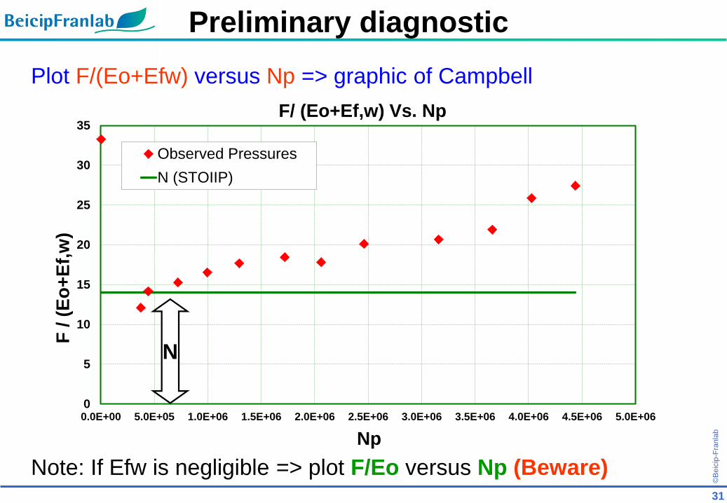
• If a reservoir has no gas-cap but might be influenced by water
influx from an aquifer, the MB equation is simplified as follows,
F = N (Eo + Efw) + We*Bw
• This can be transformed into
F / (Eo + Efw) = N + We*Bw / (Eo + Efw)
• Two unknowns N and We (right side of the equation), but the left
side is easy to calculate.
• Plot the left side versus Np [or time or p (pressure decline)]
Note: the plot originally proposed by Campbell was F/Et versus F
Preliminary diagnostic
©B
eic
ip-F
ranla
b
0
5
10
15
20
25
30
35
0.0E+00 5.0E+05 1.0E+06 1.5E+06 2.0E+06 2.5E+06 3.0E+06 3.5E+06 4.0E+06 4.5E+06 5.0E+06
F / (
Eo
+E
f,w
)
Np
F/ (Eo+Ef,w) Vs. Np
Observed Pressures
N (STOIIP)
N
31
Plot F/(Eo+Efw) versus Np => graphic of Campbell
Note: If Efw is negligible => plot F/Eo versus Np (Beware)
Preliminary diagnostic
©B
eic
ip-F
ranla
b
0
5
10
15
20
25
30
35
0.0E+00 5.0E+05 1.0E+06 1.5E+06 2.0E+06 2.5E+06 3.0E+06 3.5E+06 4.0E+06 4.5E+06 5.0E+06
F /
(E
o+
Ef,
w)
Np
F/ (Eo+Ef,w) Vs. Np
Observed Pressures
N (STOIIP)
N
32
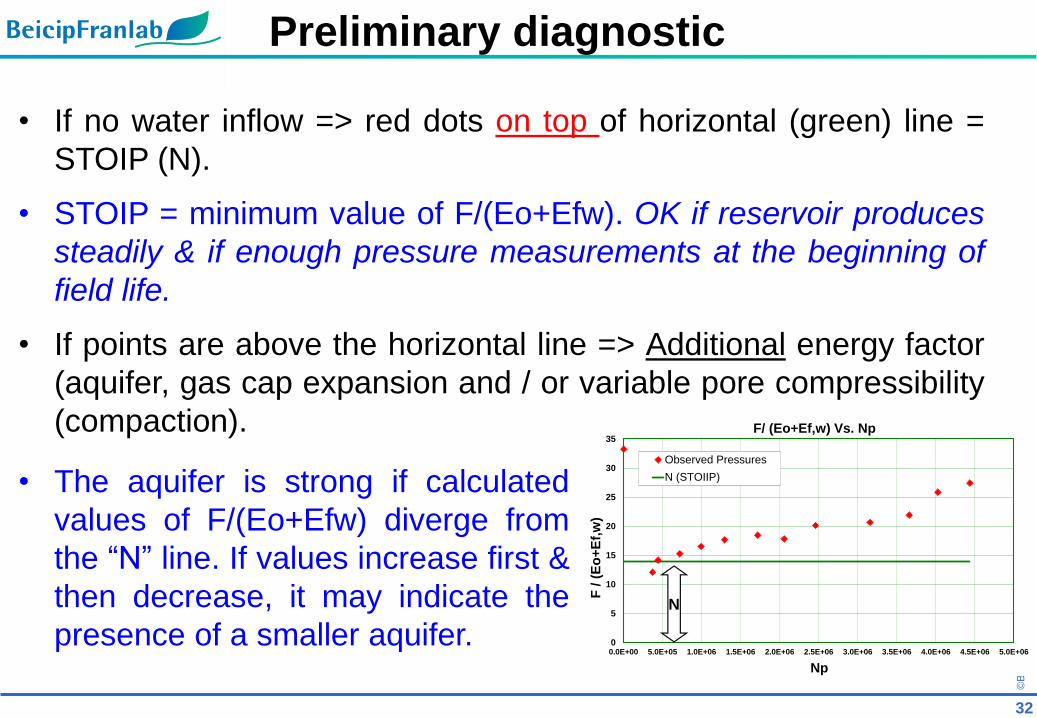
• If no water inflow => red dots on top of horizontal (green) line =
STOIP (N).
• STOIP = minimum value of F/(Eo+Efw). OK if reservoir produces
steadily & if enough pressure measurements at the beginning of
field life.
• If points are above the horizontal line => Additional energy factor
(aquifer, gas cap expansion and / or variable pore compressibility
(compaction).
• The aquifer is strong if calculated
values of F/(Eo+Efw) diverge from
the “N” line. If values increase first &
then decrease, it may indicate the
presence of a smaller aquifer.
Preliminary diagnostic
©B
eic
ip-F
ranla
b
0
5
10
15
20
25
30
35
0.0E+00 5.0E+05 1.0E+06 1.5E+06 2.0E+06 2.5E+06 3.0E+06 3.5E+06 4.0E+06 4.5E+06 5.0E+06
F / E
t
Np
F/Et Vs. Np
Observed Pressures
N (STOIIP)
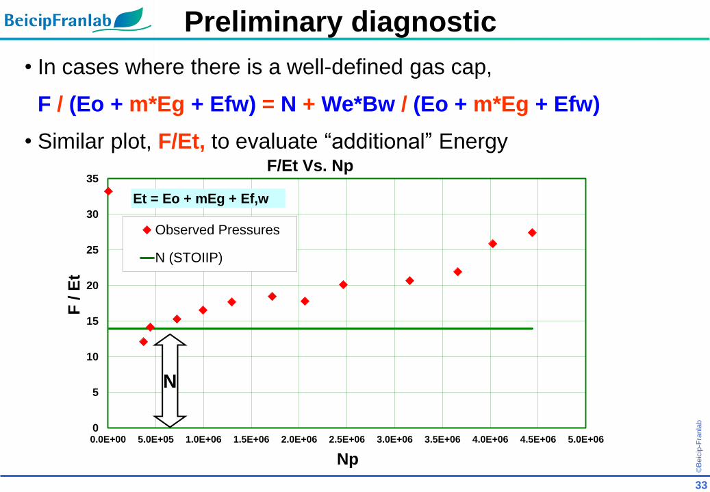
Et = Eo + mEg + Ef,w
N
33
• In cases where there is a well-defined gas cap,
F / (Eo + m*Eg + Efw) = N + We*Bw / (Eo + m*Eg + Efw)
• Similar plot, F/Et, to evaluate “additional” Energy
Preliminary diagnostic
©B
eic
ip-F
ranla
b
34
• Calculated values of F/(Eo+Efw) or F/Et cannot decrease with Np
(or time) if data are reliable.
• If it occurs => Possible communication with another reservoir.
• Decrease of F/(Eo+Efw) or F/Et => production "transferred" to a
neighbouring reservoir.
• Increase of F/(Eo+Efw) or F/Et, if there is no initial gas-cap, neither
the water influx is credible => "transfer" of fluids from another
reservoir.
Preliminary diagnostic
©B
eic
ip-F
ranla
b
35
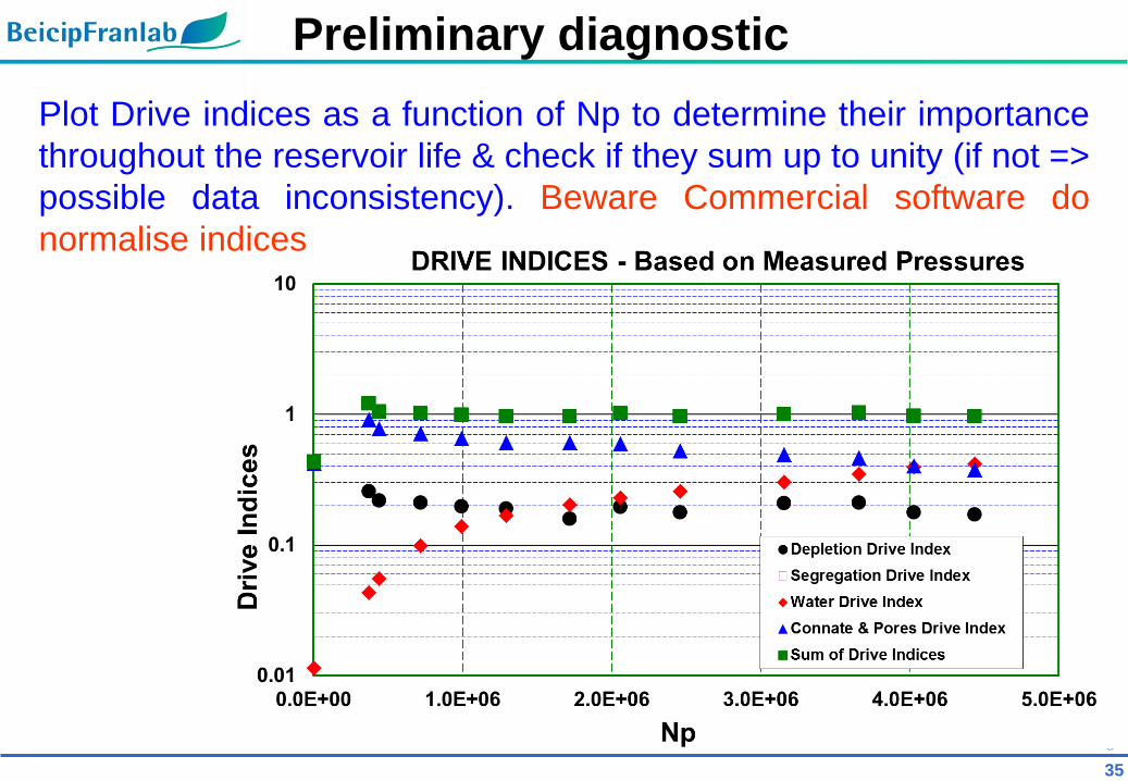
Plot Drive indices as a function of Np to determine their importance
throughout the reservoir life & check if they sum up to unity (if not =>
possible data inconsistency). Beware Commercial software do
normalise indices
Preliminary diagnostic
©B
eic
ip-F
ranla
b
36
Production Mechanisms
Reservoirs with Volumetric Depletion
©B
eic
ip-F
ranla
b
37
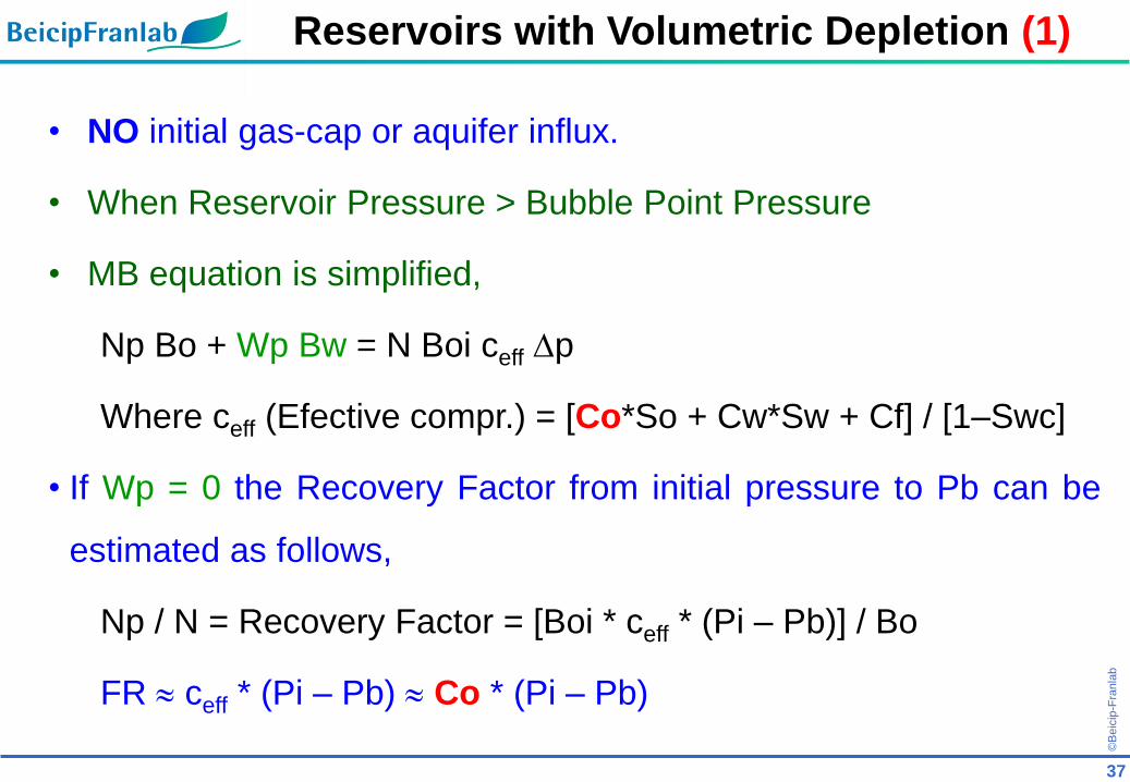
• NO initial gas-cap or aquifer influx.
• When Reservoir Pressure > Bubble Point Pressure
• MB equation is simplified,
Np Bo + Wp Bw = N Boi ceff p
Where ceff (Efective compr.) = [Co*So + Cw*Sw + Cf] / [1–Swc]
• If Wp = 0 the Recovery Factor from initial pressure to Pb can be
estimated as follows,
Np / N = Recovery Factor = [Boi * ceff * (Pi – Pb)] / Bo
FR ceff * (Pi – Pb) Co * (Pi – Pb)
Reservoirs with Volumetric Depletion (1)
©B
eic
ip-F
ranla
b
38
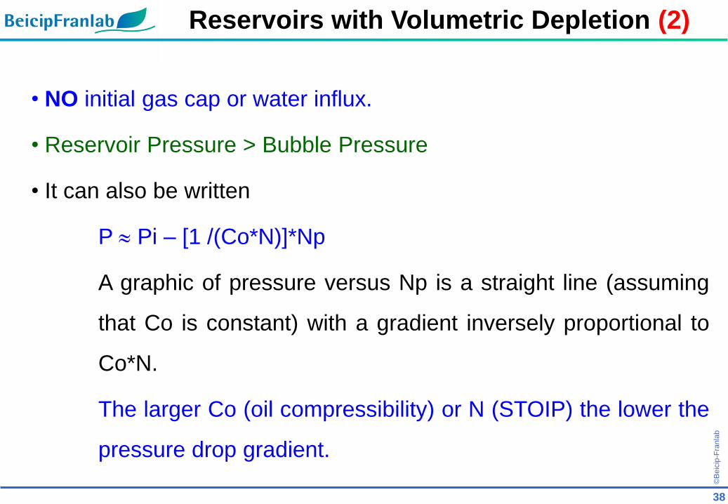
• NO initial gas cap or water influx.
• Reservoir Pressure > Bubble Pressure
• It can also be written
P Pi – [1 /(Co*N)]*Np
A graphic of pressure versus Np is a straight line (assuming
that Co is constant) with a gradient inversely proportional to
Co*N.
The larger Co (oil compressibility) or N (STOIP) the lower the
pressure drop gradient.
Reservoirs with Volumetric Depletion (2)
©B
eic
ip-F
ranla
b
39
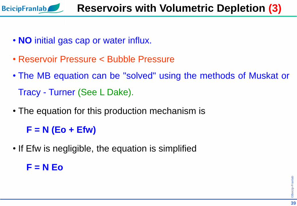
• NO initial gas cap or water influx.
• Reservoir Pressure < Bubble Pressure
• The MB equation can be "solved" using the methods of Muskat or
Tracy - Turner (See L Dake).
• The equation for this production mechanism is
F = N (Eo + Efw)
• If Efw is negligible, the equation is simplified
F = N Eo
Reservoirs with Volumetric Depletion (3)
©B
eic
ip-F
ranla
b
40
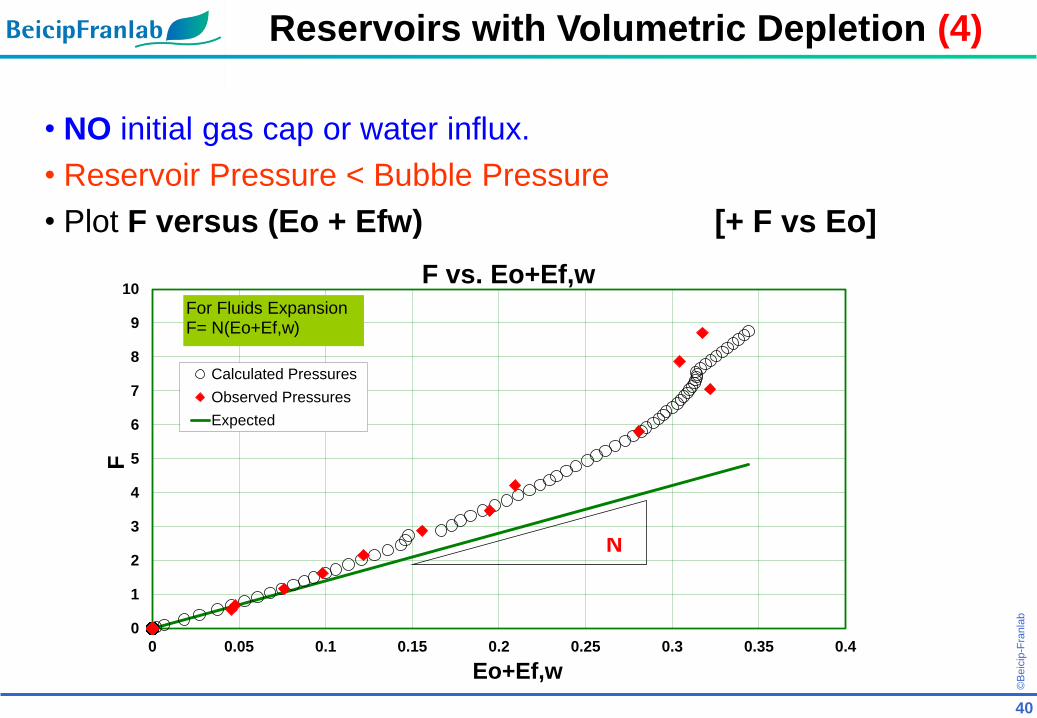
• NO initial gas cap or water influx.
• Reservoir Pressure < Bubble Pressure
• Plot F versus (Eo + Efw) [+ F vs Eo]
Reservoirs with Volumetric Depletion (4)
0
1
2
3
4
5
6
7
8
9
10
0 0.05 0.1 0.15 0.2 0.25 0.3 0.35 0.4
F
Eo+Ef,w
F vs. Eo+Ef,w
Calculated Pressures
Observed Pressures
Expected
For Fluids Expansion F= N(Eo+Ef,w)
N
©B
eic
ip-F
ranla
b
41
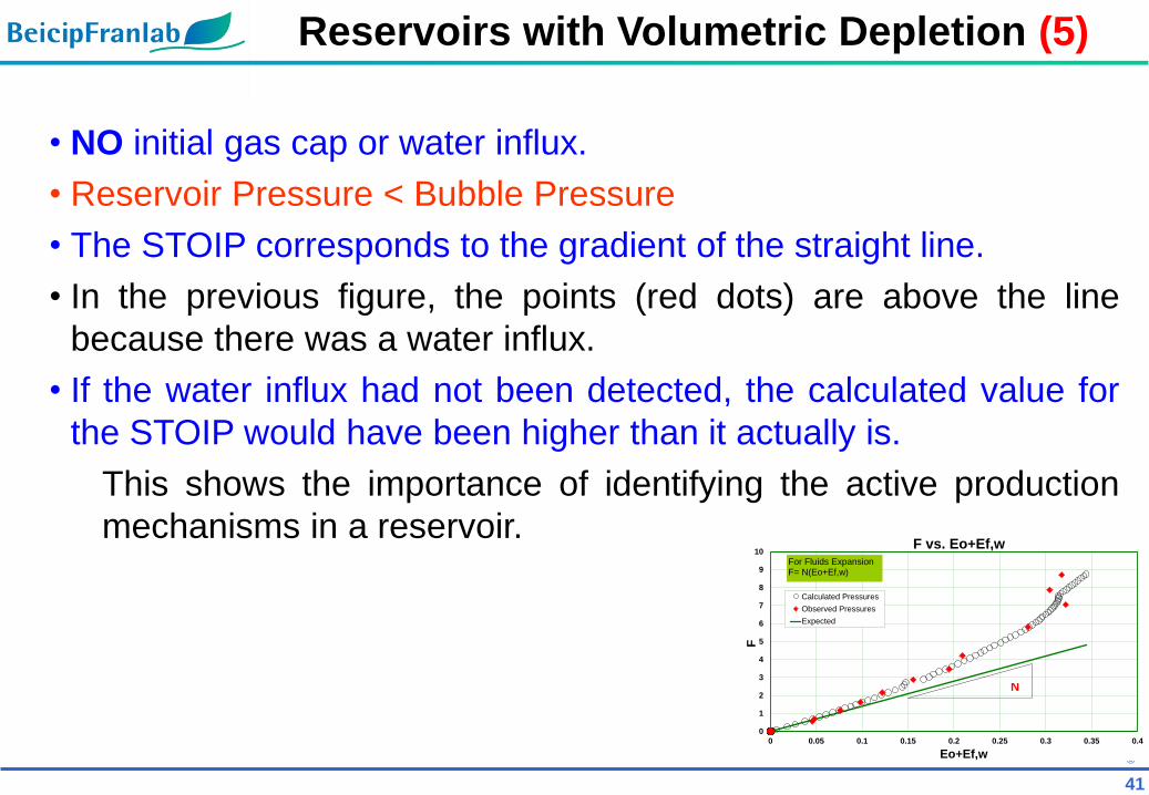
• NO initial gas cap or water influx.
• Reservoir Pressure < Bubble Pressure
• The STOIP corresponds to the gradient of the straight line.
• In the previous figure, the points (red dots) are above the line
because there was a water influx.
• If the water influx had not been detected, the calculated value for
the STOIP would have been higher than it actually is.
This shows the importance of identifying the active production
mechanisms in a reservoir.
Reservoirs with Volumetric Depletion (5)
0
1
2
3
4
5
6
7
8
9
10
0 0.05 0.1 0.15 0.2 0.25 0.3 0.35 0.4
FEo+Ef,w
F vs. Eo+Ef,w
Calculated Pressures
Observed Pressures
Expected
For Fluids Expansion F= N(Eo+Ef,w)
N
©B
eic
ip-F
ranla
b
42
Mechanisms of Production Reservoirs with Water Influx
©B
eic
ip-F
ranla
b
43
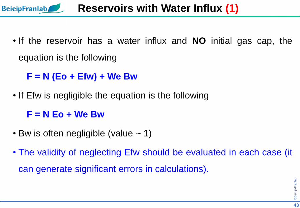
• If the reservoir has a water influx and NO initial gas cap, the
equation is the following
F = N (Eo + Efw) + We Bw
• If Efw is negligible the equation is the following
F = N Eo + We Bw
• Bw is often negligible (value ~ 1)
• The validity of neglecting Efw should be evaluated in each case (it
can generate significant errors in calculations).
Reservoirs with Water Influx (1)
©B
eic
ip-F
ranla
b
44
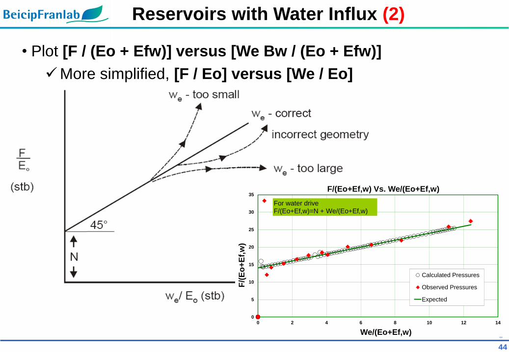
• Plot [F / (Eo + Efw)] versus [We Bw / (Eo + Efw)]
More simplified, [F / Eo] versus [We / Eo]
0
5
10
15
20
25
30
35
0 2 4 6 8 10 12 14
F/(
Eo
+E
f,w
)
We/(Eo+Ef,w)
F/(Eo+Ef,w) Vs. We/(Eo+Ef,w)
Calculated Pressures
Observed Pressures
Expected
For water drive F/(Eo+Ef,w)=N + We/(Eo+Ef,w)
Reservoirs with Water Influx (2)

©B
eic
ip-F
ranla
b
45
• If We estimate is correct, the relationship between the two
variables is a straight line,
• If We is under-estimated => Line goes up and
• If We is over-estimated => Line goes down.
• If the geometry is incorrect (radial or linear aquifer for example) the
line could have the shape shown in the figure.
• If the calculations of water influx are made
• separating the constant of influx C = 1.119fhcro2
• from the solution of Van Everdingen and Hurst for the diffusivity
equation [pQD(p,rD)]
• the slope of the straight line is C and not 45° (grad. = 1).
Reservoirs with Water Influx (3)
©B
eic
ip-F
ranla
b
46
• Calculations of water influx = Method proposed by Hurst and Van
Everdingen.
• There is an approximate solution, for the case of the unsteady-
state regime, proposed by Fetkovitch.
• Fetkovitch calculations are simple and easy to apply while the
calculations of Van Everdingen and Hurst are tedious.
• Fetkovitch calculations are implemented in most commercial
numerical simulators.
• The two methods of calculation are described in many reference
texts of reservoir engineering.
Reservoirs with Water Influx (4)
©B
eic
ip-F
ranla
b
47
Mechanisms of Production
Reservoirs with Gas Cap

©B
eic
ip-F
ranla
b
48
• If the reservoir HAS initial gas cap but NO water influx
F = N (Eo + m*Eg + Efw)
• If Efw is negligible (reasonable as cgas >> cw and cgas >> co)
F = N (Eo + m*Eg)
• Alternatively if you want to determine m and N
F / Eo = N + m*N*Eg / Eo
• These two equations provide two alternatives for the calculations
of reservoirs with gas cap.
Reservoirs with Gas Cap
©B
eic
ip-F
ranla
b
49
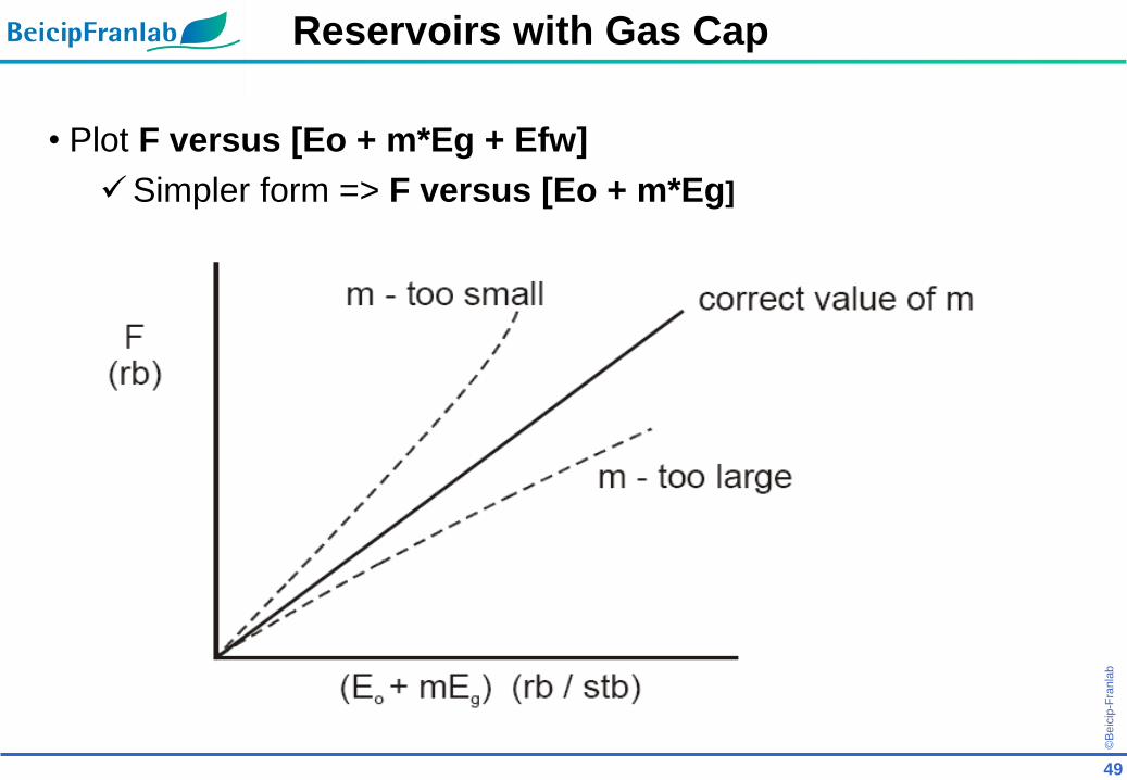
• Plot F versus [Eo + m*Eg + Efw]
Simpler form => F versus [Eo + m*Eg]
Reservoirs with Gas Cap
©B
eic
ip-F
ranla
b
50
• The straight line gradient => STOOIP (N).
• Straight line always passes through the origin of the axes
(important for the analysis).
• If the estimation of "m" is correct, the relationship between both
variables is a straight line
If “m” is under-estimated, the line goes up and
If “m” is over-estimated, the line goes down
If the reservoir has a water influx, the points are going up
regardless of the value of "m".
• This shows again the importance of a proper evaluation of the
active production mechanisms.
Reservoirs with Gas Cap

©B
eic
ip-F
ranla
b
51
• Odeh and Havlena considered that only had limited success in
determining the volume of the gas cap that needs exceptional
accuracy of data used (pressures in particular).
• Alternative graphic is F / Eo versus Eg / Eo.
Plot slope = m*N. Value of ordinate = N
Eg / Eo
F / Eo (stb)
N
mN
• The first plot has the advantage that the
line has to pass necessarily through the
origin
• While in this case, the ordinate is the
value of N (unknown).
Reservoirs with Gas Cap
©B
eic
ip-F
ranla
b
52
Mechanisms of Production
Reservoirs with Gas Cap and Water Influx
©B
eic
ip-F
ranla
b
53
• This is the most complex of all.
F = N (Eo + m*Eg + Efw) + We*Bw
• If Efw is removed (this assumption should always be verified
before being applied).
• Plot F / (Eo + m*Eg) versus N + We*Bw / (Eo + m*Eg)
• Bw can be neglected if it is close to 1.
• The interpretation of this graphic is similar to the graphic used for
the water influx with the significant difference that there is an
additional parameter to determine m.
Reservoirs with Gas Cap & Water Influx
©B
eic
ip-F
ranla
b
54
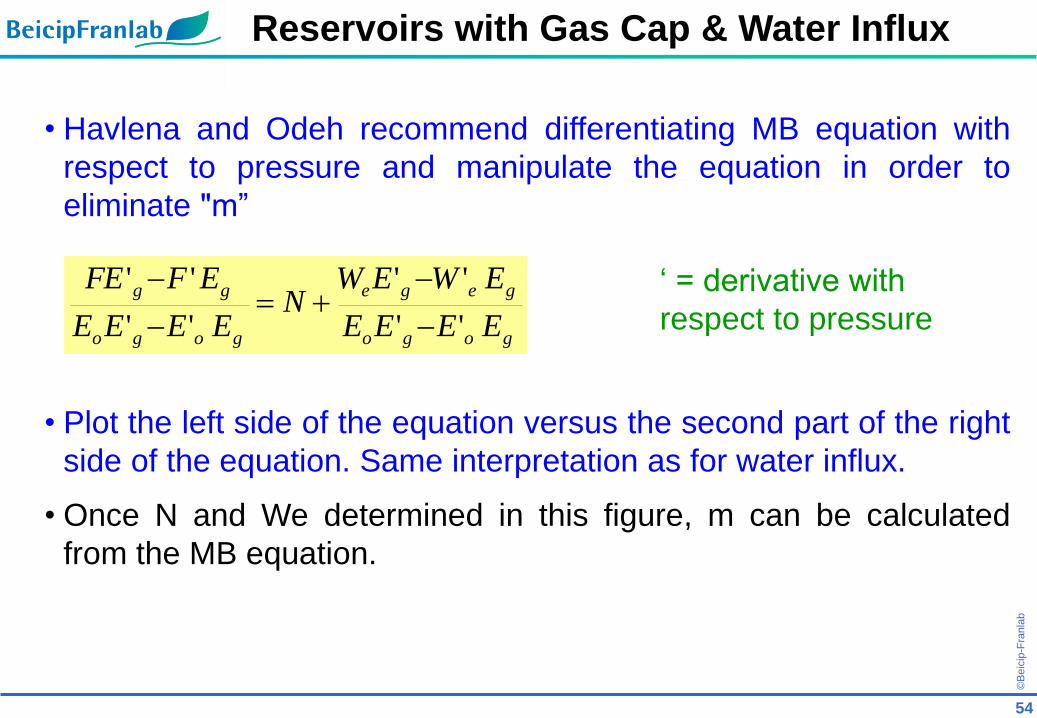
• Havlena and Odeh recommend differentiating MB equation with
respect to pressure and manipulate the equation in order to
eliminate "m”
• Plot the left side of the equation versus the second part of the right
side of the equation. Same interpretation as for water influx.
• Once N and We determined in this figure, m can be calculated
from the MB equation.
gogo
gege
gogo
gg
EEEE
EWEWN
EEEE
EFFE
''
''
''
''
Reservoirs with Gas Cap & Water Influx
‘ = derivative with
respect to pressure
©B
eic
ip-F
ranla
b
55
Conclusion
©B
eic
ip-F
ranla
b
56
• Identify production mechanisms prior to numerical simulation.
• To identify mechanisms => use Havlena and Odeh plots
• Dake thought difficult to develop a software to cover all situations
for which MB calculations are applied.
Conclusions / recommendations
©B
eic
ip-F
ranla
b
57
THANK YOU VERY
MUCH
![Index [] a Abbasov/Romo’s Diels–Alder lactonization 628 ab initio – calculations 1159 – molecular orbital calculations 349 – wavefunction 209](https://img.pdfslide.tips/doc/110x75/5aad6f3f7f8b9aa9488e42ac/index-a-abbasovromos-dielsalder-lactonization-628-ab-initio-calculations.jpg)