Embed Size (px)
Citation preview
7/31/2019 Mehmet Tez
http://slidepdf.com/reader/full/mehmet-tez 1/95
APPLYING FORMAL CONTROL THEORETIC TECHNIQUES TO COMPUTERSYSTEM PERFORMANCE MANAGEMENT
BY
MEHMET HADI SUZER
BS, Inonu University, 2003
MS, Binghamton University, 2007
DISSERTATION
Submitted in partial fulfillment of the requirements for
the degree of Doctor of Philosophy in Computer Sciencein the Graduate School of Binghamton University
State University of New York2011

7/31/2019 Mehmet Tez
http://slidepdf.com/reader/full/mehmet-tez 2/95
All rights reserved
INFORMATION TO ALL USERSThe quality of this reproduction is dependent on the quality of the copy submitted.
In the unlikely event that the author did not send a complete manuscriptand there are missing pages, these will be noted. Also, if material had to be removed,
a note will indicate the deletion.
All rights reserved. This edition of the work is protected againstunauthorized copying under Title 17, United States Code.
ProQuest LLC.789 East Eisenhower Parkway
P.O. Box 1346
Ann Arbor, MI 48106 - 1346
UMI 3469608
Copyright 2011 by ProQuest LLC.
UMI Number: 3469608

7/31/2019 Mehmet Tez
http://slidepdf.com/reader/full/mehmet-tez 3/95
cCopyright by Mehmet Hadi Suzer 2011
All Rights Reserved
7/31/2019 Mehmet Tez
http://slidepdf.com/reader/full/mehmet-tez 4/95
Accepted in partial fullfillment of the requirements forthe degree of Doctor of Philosophy in Computer Science
in the Graduate School of Binghamton University
State University of New York2011
August 5, 2011
Dr. Kyoung-Don Kang, Chair and Faculty AdvisorDepartment of Computer Science, Binghamton University
Dr. Leslie Lander, MemberDepartment of Computer Science, Binghamton University
Dr. Kartik Gopalan, MemberDepartment of Computer Science, Binghamton University
Dr. Edward Li, Outside ExaminerDepartment of Electrical and Computer Engineering, Binghamton University
iii
7/31/2019 Mehmet Tez
http://slidepdf.com/reader/full/mehmet-tez 5/95
Abstract
Computer systems have limited amounts of resources to serve applications’ growing
demands. Most systems tend to allocate resources to applications by of fline analysis of ap-
plication requirements, which often results in inef ficient resource usage due to the dynamic,
time-varying nature of workloads. Formal control theory is known to effectively support
the desired performance of the controlled system. However, it is challenging to support the
performance of computational systems, since there is no definitive methodology to model
computer system dynamics unlikephysics laws applied to model physical systems such as a
cruise control system. Modeling computer systems, selecting proper control theoretic tools
and tuning them according to the needs of specific applications - the research problems to
be investigated in this proposed work- are the key ingredients for successful application of
control theory to computer system performance management.
To support the desired system performance even in the presence of dynamic work-
loads, we have applied advanced control theoretic approaches, namely fuzzy control theory,
model predictive control theory and event-driven control theoretic techniques. Specifically,
we apply these techniques to manage the CPU utilization in a real-time operating system,
network bandwidth consumption for video streaming, and link congestion in network gate-
ways.
I aim to demonstrate the applicability of formal control theoretic techniques to sup-port desired system behaviors even in the presence of dynamic workloads and uncertain
environments. In this way, I intend to improve the predictability and reliability of computer
systems that need to process highly dynamic workloads in uncertain environments.
iv
7/31/2019 Mehmet Tez
http://slidepdf.com/reader/full/mehmet-tez 6/95
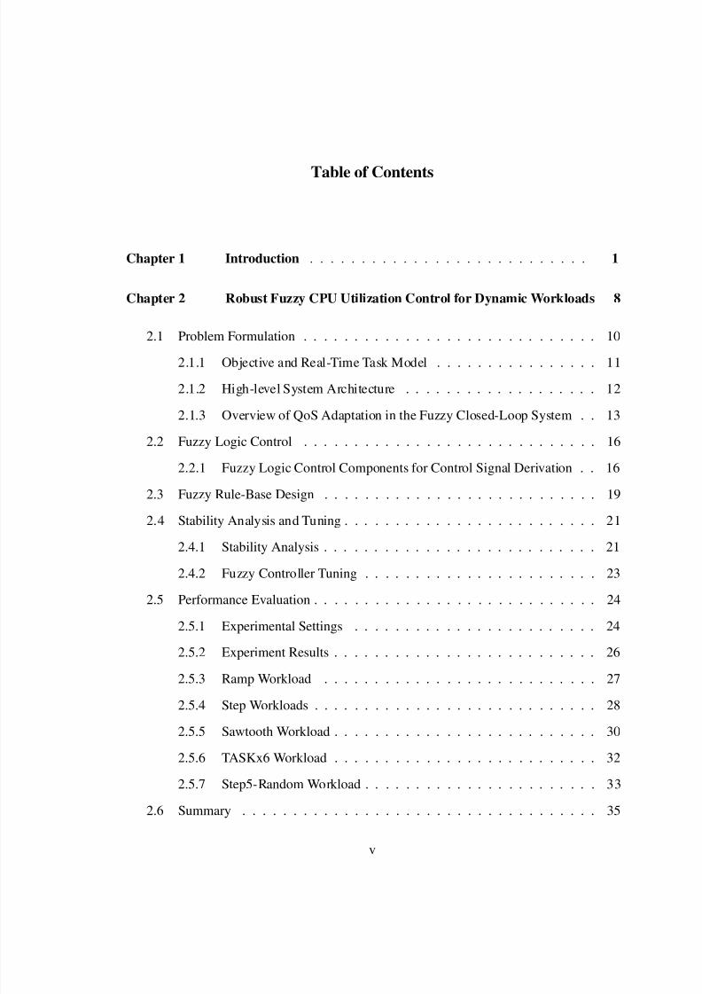
Table of Contents
Chapter 1 Introduction . . . . . . . . . . . . . . . . . . . . . . . . . . . 1
Chapter 2 Robust Fuzzy CPU Utilization Control for Dynamic Workloads 8
2.1 Problem Formulation . . . . . . . . . . . . . . . . . . . . . . . . . . . . . 10
2.1.1 Objective and Real-Time Task Model . . . . . . . . . . . . . . . . 11
2.1.2 High-level System Architecture . . . . . . . . . . . . . . . . . . . 12
2.1.3 Overview of QoS Adaptation in the Fuzzy Closed-Loop System . . 13
2.2 Fuzzy Logic Control . . . . . . . . . . . . . . . . . . . . . . . . . . . . . 16
2.2.1 Fuzzy Logic Control Components for Control Signal Derivation . . 16
2.3 Fuzzy Rule-Base Design . . . . . . . . . . . . . . . . . . . . . . . . . . . 19
2.4 Stability Analysis and Tuning . . . . . . . . . . . . . . . . . . . . . . . . . 21
2.4.1 Stability Analysis . . . . . . . . . . . . . . . . . . . . . . . . . . . 21
2.4.2 Fuzzy Controller Tuning . . . . . . . . . . . . . . . . . . . . . . . 23
2.5 Performance Evaluation . . . . . . . . . . . . . . . . . . . . . . . . . . . . 24
2.5.1 Experimental Settings . . . . . . . . . . . . . . . . . . . . . . . . 24
2.5.2 Experiment Results . . . . . . . . . . . . . . . . . . . . . . . . . . 26
2.5.3 Ramp Workload . . . . . . . . . . . . . . . . . . . . . . . . . . . 27
2.5.4 Step Workloads . . . . . . . . . . . . . . . . . . . . . . . . . . . . 28
2.5.5 Sawtooth Workload . . . . . . . . . . . . . . . . . . . . . . . . . . 30
2.5.6 TASKx6 Workload . . . . . . . . . . . . . . . . . . . . . . . . . . 32
2.5.7 Step5-Random Workload . . . . . . . . . . . . . . . . . . . . . . . 33
2.6 Summary . . . . . . . . . . . . . . . . . . . . . . . . . . . . . . . . . . . 35
v
7/31/2019 Mehmet Tez
http://slidepdf.com/reader/full/mehmet-tez 7/95
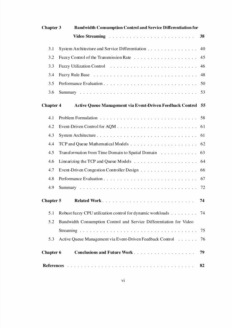
Chapter 3 Bandwidth Consumption Control and Service Differentiation for
Video Streaming . . . . . . . . . . . . . . . . . . . . . . . . . 38
3.1 System Architecture and Service Differentiation . . . . . . . . . . . . . . . 40
3.2 Fuzzy Control of the Transmission Rate . . . . . . . . . . . . . . . . . . . 45
3.3 Fuzzy Utilization Control . . . . . . . . . . . . . . . . . . . . . . . . . . 46
3.4 Fuzzy Rule Base . . . . . . . . . . . . . . . . . . . . . . . . . . . . . . . 48
3.5 Performance Evaluation . . . . . . . . . . . . . . . . . . . . . . . . . . . . 50
3.6 Summary . . . . . . . . . . . . . . . . . . . . . . . . . . . . . . . . . . . 53
Chapter 4 Active Queue Management via Event-Driven Feedback Control 55
4.1 Problem Formulation . . . . . . . . . . . . . . . . . . . . . . . . . . . . . 58
4.2 Event-Driven Control for AQM . . . . . . . . . . . . . . . . . . . . . . . . 61
4.3 System Architecture . . . . . . . . . . . . . . . . . . . . . . . . . . . . . . 61
4.4 TCP and Queue Mathematical Models . . . . . . . . . . . . . . . . . . . . 62
4.5 Transformation from Time Domain to Spatial Domain . . . . . . . . . . . 63
4.6 Linearizing the TCP and Queue Models . . . . . . . . . . . . . . . . . . . 64
4.7 Event-Driven Congestion Controller Design . . . . . . . . . . . . . . . . . 66
4.8 Performance Evaluation . . . . . . . . . . . . . . . . . . . . . . . . . . . . 67
4.9 Summary . . . . . . . . . . . . . . . . . . . . . . . . . . . . . . . . . . . 72
Chapter 5 Related Work . . . . . . . . . . . . . . . . . . . . . . . . . . . 74
5.1 Robust fuzzy CPU utilization control for dynamic workloads . . . . . . . . 74
5.2 Bandwidth Consumption Control and Service Differentiation for Video
Streaming . . . . . . . . . . . . . . . . . . . . . . . . . . . . . . . . . . . 75
5.3 Active Queue Management via Event-Driven Feedback Control . . . . . . 76
Chapter 6 Conclusions and Future Work . . . . . . . . . . . . . . . . . . 79
References . . . . . . . . . . . . . . . . . . . . . . . . . . . . . . . . . . . . . 82
vi
7/31/2019 Mehmet Tez
http://slidepdf.com/reader/full/mehmet-tez 8/95
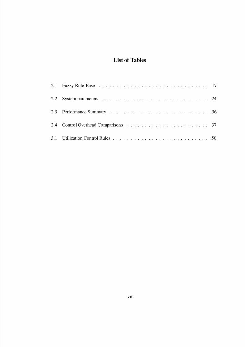
List of Tables
2.1 Fuzzy Rule-Base . . . . . . . . . . . . . . . . . . . . . . . . . . . . . . . 17
2.2 System parameters . . . . . . . . . . . . . . . . . . . . . . . . . . . . . . 24
2.3 Performance Summary . . . . . . . . . . . . . . . . . . . . . . . . . . . . 36
2.4 Control Overhead Comparisons . . . . . . . . . . . . . . . . . . . . . . . 37
3.1 Utilization Control Rules . . . . . . . . . . . . . . . . . . . . . . . . . . . 50
vii
7/31/2019 Mehmet Tez
http://slidepdf.com/reader/full/mehmet-tez 9/95
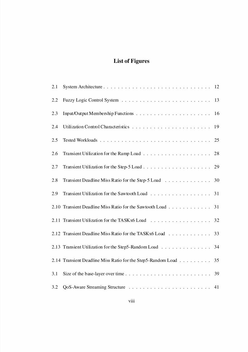
List of Figures
2.1 System Architecture . . . . . . . . . . . . . . . . . . . . . . . . . . . . . . 12
2.2 Fuzzy Logic Control System . . . . . . . . . . . . . . . . . . . . . . . . . 13
2.3 Input/Output Membership Functions . . . . . . . . . . . . . . . . . . . . . 16
2.4 Utilization Control Characteristics . . . . . . . . . . . . . . . . . . . . . . 19
2.5 Tested Workloads . . . . . . . . . . . . . . . . . . . . . . . . . . . . . . . 25
2.6 Transient Utilization for the Ramp Load . . . . . . . . . . . . . . . . . . . 28
2.7 Transient Utilization for the Step-5 Load . . . . . . . . . . . . . . . . . . . 29
2.8 Transient Deadline Miss Ratio for the Step-5 Load . . . . . . . . . . . . . 30
2.9 Transient Utilization for the Sawtooth Load . . . . . . . . . . . . . . . . . 31
2.10 Transient Deadline Miss Ratio for the Sawtooth Load . . . . . . . . . . . . 31
2.11 Transient Utilization for the TASKx6 Load . . . . . . . . . . . . . . . . . 32
2.12 Transient Deadline Miss Ratio for the TASKx6 Load . . . . . . . . . . . . 33
2.13 Transient Utilization for the Step5-Random Load . . . . . . . . . . . . . . 34
2.14 Transient Deadline Miss Ratio for the Step5-Random Load . . . . . . . . . 35
3.1 Size of the base-layer over time . . . . . . . . . . . . . . . . . . . . . . . . 39
3.2 QoS-Aware Streaming Structure . . . . . . . . . . . . . . . . . . . . . . . 41
viii
7/31/2019 Mehmet Tez
http://slidepdf.com/reader/full/mehmet-tez 10/95
3.3 Multi-Hop qVSF System . . . . . . . . . . . . . . . . . . . . . . . . . . . 44
3.4 Fuzzy Controller . . . . . . . . . . . . . . . . . . . . . . . . . . . . . . . 46
3.5 Membership Functions . . . . . . . . . . . . . . . . . . . . . . . . . . . . 46
3.6 Utilization Control Characteristics . . . . . . . . . . . . . . . . . . . . . . 49
3.7 Transient and average bandwidth consumption (4 streams) . . . . . . . . . 51
3.8 Average number of transmitted enhancement layers per stream . . . . . . . 52
3.9 Number of transmitted enhancement layers per stream . . . . . . . . . . . 53
3.10 Scenes with different priorities . . . . . . . . . . . . . . . . . . . . . . . . 54
4.1 System Architecture . . . . . . . . . . . . . . . . . . . . . . . . . . . . . . 61
4.2 Test Bed . . . . . . . . . . . . . . . . . . . . . . . . . . . . . . . . . . . . 67
4.3 Queue Lengths . . . . . . . . . . . . . . . . . . . . . . . . . . . . . . . . 69
4.4 E2E Delays . . . . . . . . . . . . . . . . . . . . . . . . . . . . . . . . . . 70
4.5 Packet Drop Rates . . . . . . . . . . . . . . . . . . . . . . . . . . . . . . . 71
4.6 Activation Frequencies . . . . . . . . . . . . . . . . . . . . . . . . . . . . 72
ix
7/31/2019 Mehmet Tez
http://slidepdf.com/reader/full/mehmet-tez 11/95
Chapter 1
Introduction
Computer systems have limited amounts of resources to serve applications’ growing
demands. Most systems tend to allocate resources to applications by of fline analysis of ap-
plication requirements, which often results in inef ficient resource usage due to the dynamic,
time-varying nature of workloads. Formal control theory is known to effectively support
the desired performance of the controlled system. However, it is challenging to support the
performance of computational systems, since there is no definitive methodology to model
computer system dynamics unlike physics laws applied to model physical systems such as
a cruise control system.
Modeling computer systems, selecting proper control theoretic tools and tuning them
according to the needs of specific applications -the research problems to be investigated
in this proposed work- are the key ingredients for successful application of control theory
to computer system performance management. To support desired system performance
even in the presence of dynamic workloads, we have applied advanced control theoretic
approaches, namely fuzzy control theory, model predictive control theory and event-driven
control theoretic techniques. Specifically, we apply these techniques to manage the CPU
utilization in a real-time operating system, network bandwidth consumption for video
streaming, and link congestion in network gateways.
First, to reduce the dif ficulty of modeling real-time systems with stringent timing con-
straints, we apply formal fuzzy control theory that is very effective to support the desired
performance in a nonlinear dynamic system without requiring a system model. Traditional
real-time scheduling techniques [29] requiring precise a priori knowledge of the workload
1
7/31/2019 Mehmet Tez
http://slidepdf.com/reader/full/mehmet-tez 12/95
are not directly applicable to support timing constraints. Thus, it is critical to continuously
measure and control the utilization in a feedback loop to avoid severe underutilization or
overload in real-time systems operating in dynamic environments. Linear PID (propor-
tional, integral, and differential) control techniques [41] have been applied to manage real-
time performance in dynamic environments [3, 31]. However, PID controllers and their
variants, e.g., P, PI, or PD controllers, usually approximate the system dynamics in a piece-
wise linear fashion [16,31]. PID controllers are guaranteed to support the set-point only
if system dynamics do not deviate from a specific operating range derived of fline. If the
workload varies dynamically exceeding the operating range, PID controllers and their vari-
ants, may largely fail to support the set-point [16]. Model predictive control theory [34] is
applied to manage the utilization in dynamic environments by continuously modeling the
system behavior online [32,50]. However, approximate models are often used to reduce the
complexity of online predictive modeling of the controlled real-time system. For example,
the authors of [32, 50] assume that the actual execution times of real-time tasks are equal
to their estimated execution times to decrease the complexity of system modeling. Also,
the predictive system model derived online may have non-trivial errors when workloads
change fast [4].
In this chapter, we apply formal fuzzy logic control theory [39] to adapt workloads, if
necessary, to make the utilization converge to the specified set-point even given dynamic
workloads. Unlike PID and model predictive control techniques, fuzzy control is not tied
to a mathematical model of the controlled system or an operating range. We support direct
nonlinear mappings between the utilization error (= target utilization − current utilization)
and the workload adjustment required to achieve the target utilization via IF-THEN rules.
Rather than relying on an approximate system model, we develop a novel fuzzy closed-loopsystem to control the utilization based on the logical understanding of the relation between
the workload and utilization changes.
Via the Lyapunov direct method [4, 39], we mathematically prove the stability of the
fuzzy closed-loop system. Further, we extend the Real-Time Application Interface (RTAI)
for Linux kernel [43]. We implement and evaluate our fuzzy logic utilization controller as
2
7/31/2019 Mehmet Tez
http://slidepdf.com/reader/full/mehmet-tez 13/95
well as two existing utilization controllers based on the linear and model predictive con-
trol theory for an extensive set of workloads in RTAI. Among the tested approaches, our
approach shows the smallest deviation from and the fastest convergence to the specified
utilization set-point when the system is in a transient status.
Second, we applied fuzzy control theory to network bandwidth consumed by multi-
media streaming. In this way, we aim to avoid undesirable situations in which multimedia
streaming starves other applications such as file transfer sharing the network, for example,
in a smart home. To bound the bandwidth usage of streaming, we leverage the layered en-
coding technique, in which a video frame consists of a base layer and multiple enhancement
layers. We always transmit the base layer, because it is required to display a scene. How-
ever, under overload, we degrade the video quality by dropping high enhancement layers
without affecting the underlying layers, if necessary, to support the specified bit rate bound.
A key challenge is how to determine how many enhancement layers to transmit for con-
current video streams to support the specified bit rate bound. This is not a trivial problem,
since the size of a frame consisting of a base layer and enhancement layers may signifi-
cantly vary in time depending on the complexity of the scenes and their inter-relations in
a video. Additionally, new multimedia streaming sessions may start, while others may ter-
minate, further increasing the complexity of bit rate control. We also differentiate the video
quality for streams with different levels of importance. We have implemented our transmis-
sion rate control and service differentiation schemes and evaluated them in our department
network where a number of different applications may coexist at the same time.
In this chapter, we present our QoS-aware video streaming framework (qVSF) imple-
mented on top of an open source video streaming server, QStream [42]. We apply fuzzylogic control to support the specified end-to-end bit rate bound at the node with the bot-
tleneck link that suffers the most significant network congestion, since it may have the
lowest physical bandwidth and/or the largest amount of streaming data to deliver. The
controller at the bottleneck node informs streaming servers, i.e., stream data sources, how
many enhancement layers they can transmit during the next sampling period. If streams
3
7/31/2019 Mehmet Tez
http://slidepdf.com/reader/full/mehmet-tez 14/95
going through the bottleneck link have different levels of importance, qVSF differentiates
the service by allowing more important stream sources to transmit more enhancement lay-
ers. To this end, we apply fuzzy control theory, since it is known to be very effective to
support the desired performance when the system model is complex and nonlinear [39].
For performance evaluation, we have run experiments across the shared department
network in the Department of Computer Science at SUNY Binghamton where a consider-
able number of different applications usually coexist at the same time. Performance evalu-
ation results show that our video streaming system can support the specified bit rate bound
and differentiate the service to ef ficiently utilize the limited bandwidth without severely
degrading the visual quality of low priority video streams.
Third, we applied formal event-driven control theory to address the congestion control
problem in gateways. Packets injected into the network by a source can be dropped before
reaching their destinations due to congestion, wasting all the resources consumed by them.
It is known that, in an extreme case, congestion collapse may happen causing users suf-
fer severe network performance degradation [20]. Active Queue Management (AQM) is
investigated to avoid incipient congestion in gateways to complement congestion control
run by the transport layer protocol such as the TCP. Usually, AQM is implemented in gate-
ways that can distinguish between the propagation delay and persistent queuing delay for
effective congestion detection. As a gateway is shared by many active connections with a
wide range of round trip times, delay tolerances, and throughput requirements, decisions
about the duration and magnitude of transient congestion to be allowed at the gateway are
best made by the gateway itself. Most existing work on AQM is either ad-hoc event-driven
feedback approaches or time-driven formal control theoretic approaches. Ad-hoc event-driven approaches for congestion control, such as RED (Random Early Detection), lack a
mathematical model therefore it is dif ficult to analyze its dynamics and tune its numerous
parameters, while time-driven control theoretic approaches sample the queue length and
run the AQM algorithm at every fixed time interval. A time-driven approach for feedback-
based congestion control may not be adaptive enough to an abrupt load surge, if a low
4
7/31/2019 Mehmet Tez
http://slidepdf.com/reader/full/mehmet-tez 15/95
sampling rate for feedback control is used or a large number of packets arrive in a short
time period that is shorter than the sampling period. To avoid this problem, a short sam-
pling period should be selected based on pessimistic assumptions about the network load.
As a result, the controller is executed unnecessarily often when the load is not high, wasting
precious resources at the gateway.
To seamlessly integrate the advantages of both event-driven and time-driven control-
theoretic approaches, we present an event-driven feedback control approach based on for-
mal control theory [15, 40]. The key idea of our approach is to design a feedback-based
congestion controller that is invoked upon the arrivals of a specified number of packets
rather than being invoked at every fixed sampling period. As our approach is based on a
mathematical model, its performance is easier to analyze and more predictable than ad-hoc
event-driven approaches are. If a large number of packets arrive in a short time interval,
event-driven controller autonomously executes more often. In this way, the latency for con-
gestion control reduces, enhancing the reactiveness to bursty network loads. In contrast,
a time-driven controller has to wait until the next sampling period even in the presence
of a dramatic increase in packet arrivals during the current sampling period. If the packet
arrival rate decreases, the event-driven controller automatically adapts itself to execute less
frequently. As a result, under light loads, it consumes less computational resources than a
time-driven controller does.
We thoroughly evaluate the performance of our approach via an extensive simulation
study in OMNeT++ [37]. We compare it to five advanced approaches for AQM: (1) RED
[13] with the ’gentle’ parameter turned on, (2) the time-driven feedback-based Proportional
Integral (PI) congestion controller developed by Hollot et al.[19], (3) Proportional Integral
based series compensation, and Position feedback compensation (PIP) Controller [17], (4)Adaptive Optimized Proportional Controller (AOPC) [49] and (5) Fuzzy Logic Controller
(FLC) [10]. The simulation results show that our event-driven controller effectively main-
tains the queue length around the specified reference, while reducing queue length fluctu-
ations compared to the tested baseline approaches. At the same time, it achieves shorter
E2E (end-to-end) delays and noticeably smaller E2E delay fluctuations than RED, PI and
5
7/31/2019 Mehmet Tez
http://slidepdf.com/reader/full/mehmet-tez 16/95
PIP controllers, while achieving almost the same E2E delays and E2E delay fluctuations
with AOPC and FLC controllers. Further, it is invoked only 8 times per second on average.
In contrast, RED is activated 30 times/s in average while PI [19], PIP [17], AOPC [49] and
FLC [10] congestion controllers are activated 160 times/s.
In summary, I aim to demonstrate the applicability of formal control theoretic tech-
niques to support desired system behaviors even in the presence of dynamic workloads
and uncertain environments. In this way, I intend to improve the predictability and reli-
ability of computer systems that need to process highly dynamic workloads in uncertain
environments.
As of August 2011, we published the following papers. In these papers, we applied
formal control theoretic techniques to computer system performance management:
• M. H. Suzer, K. D. Kang, ”Adaptive Fuzzy Control for Utilization Management”,
IEEE International Symposium on Object, Component Service Oriented Real-time
Distributed Computing (ISORC ’08), May 5-7, 2008, Orlando Florida.
• C. Basaran, K. D. Kang, M. H. Suzer, K. S. Chung, H. R. Lee, K. R. Park, ”Band-
width Consumption Control and Service Differentiation for Video Streaming,” 17th
International Conference on Computer Communications and Networks, August 3 -
7, 2008, St. Thomas U.S. Virgin Islands. (Best Paper Award Candidate)
• C. Basaran, M. H. Suzer, K. D. Kang, X. Liu, ”Robust Fuzzy CPU Utilization Control
for Dynamic Workloads”, Journal of Systems and Software, Volume 83, Issue 7, July
2010, Pages 1192-1204.
• C. Basaran, M. H. Suzer, K. D. Kang, X. Liu, ”Model-Free Fuzzy Control of CPU
Utilization for Unpredictable Workloads”, In Proceedings of the Fourth International
Workshop on Feedback Control Implementation and Design in Computing Systems
and Networks (in conjunction with the Cyber Physical Systems Week 2009), April
16, 2009, San Francisco, California, USA.
6

7/31/2019 Mehmet Tez
http://slidepdf.com/reader/full/mehmet-tez 17/95
• C. Basaran, K. D. Kang, M. H. Suzer ”Hop-by-Hop Congestion Control and Load
Balancing in Wireless Sensor Networks”, International Conference on Networks -
2010.
Also, the following paper is under review:
• M. H. Suzer, K. D. Kang, C. Basaran, ”Active Queue Management via Event-Driven
Feedback Control”, Submitted to Elsevier Computer Communications Journal.
7
7/31/2019 Mehmet Tez
http://slidepdf.com/reader/full/mehmet-tez 18/95
Chapter 2
Robust Fuzzy CPU Utilization Control for Dynamic Workloads
Real-time systems are deployed in mission critical applications such as target track-
ing, traf fic control, and electric grid management where the workload may dynamically
vary [6,30]. For example, the execution times of real-time tasks for target tracking or
traf fic control may vary significantly when the number of targets or traf fic density dynami-
cally changes. In these systems, traditional real-time scheduling techniques [29] requiring
precise a priori knowledge of the workload are not directly applicable to support timing
constraints. Thus, it is critical to continuously measure and control the utilization in a feed-
back loop to avoid severe underutilization or overload in real-time systems operating in
dynamic environments.
Linear PID (proportional, integral, and differential) control techniques [41] have been
applied to manage real-time performance in dynamic environments [3, 31]. However, PID
controllers and their variants, e.g., P, PI, or PD controllers, usually approximate the system
dynamics in a piecewise linear fashion [16,31]. PID controllers are guaranteed to support
the set-point only if system dynamics do not deviate from a specific operating range derived
of fline. If the workload varies dynamically exceeding the operating range, PID controllers
and their variants, may largely fail to support the set-point [16].
Model predictive control theory [34] is applied to manage the utilization in dynamic
environments by continuously modeling the system behavior online [32, 50]. However,
approximate models are often used to reduce the complexity of online predictive modeling
of the controlled real-time system. For example, the authors of [32, 50] assume that the
actual execution times of real-time tasks are equal to their estimated execution times to
8
7/31/2019 Mehmet Tez
http://slidepdf.com/reader/full/mehmet-tez 19/95
decrease the complexity of system modeling. Also, the predictive system model derived
online may have non-trivial errors when workloads change fast [4].
In this chapter, we apply formal fuzzy logic control theory [39] to adapt workloads, if
necessary, to make the utilization converge to the specified set-point even given dynamic
workloads. Unlike PID and model predictive control techniques, fuzzy control is not tied
to a mathematical model of the controlled system or an operating range. Because of the
model-free nature of a fuzzy logic controller, there is less risk of introducing design errors
due to, for example, statistical inaccuracies existing in a black-box plant model [34, 41].
Rather than relying on an approximate system model, we develop novel fuzzy closed-
loop system to control the utilization based on the logical understanding of the relation
between the workload and utilization changes. Intuitively, it is clear that the utilization
increases as the load increases before it saturates at 1 and vice versa. After the utilization
saturates at 1, any further load increase does not affect the utilization. In this chapter,
we develop a fuzzy logic utilization controller based on the logical understanding of the
nonlinear relation between utilization and load changes. We prove the stability of our fuzzy
logic controller via the Lyapunov direct method [4, 39]. By leveraging the stability analysis
result, we also tune the fuzzy logic controller to avoid repetitive tuning and testing.
For fair and realistic performance evaluation, we extend the Real-Time Application
Interface (RTAI) for Linux kernel [43] to implement our fuzzy logic utilization controller
(FLC), the PI utilization controller (PIC) designed via an of fline piecewise linear approxi-
mation of system dynamics [31], and the advanced model predictive utilization controller
(MPC) [32]. By performing extensive experiments, we thoroughly compare their perfor-
mance with each other. Among the tested approaches, the FLC shows the smallest deviation
from and the fastest convergence to the specifi
ed utilization set-point when the system is ina transient status. Further, it only consumes 0.53% CPU utilization and a small amount of
memory to store fuzzy rules and a few control variables.
Despite the effectiveness of fuzzy logic control theory, little prior work has been done
to apply it to manage the performance of real-time systems [26, 45]. A summary of the key
contributions of this study follows:
9
7/31/2019 Mehmet Tez
http://slidepdf.com/reader/full/mehmet-tez 20/95
• This study presents a new closed-loop approach to supporting the specified set-point
utilization even in the presence of dynamic workloads. Especially, we directly man-
age the nonlinear relation between the load and utilization via formal fuzzy logic
control theory that is very effective to support the desired performance in nonlinear,
dynamic systems [39].
• Unlike the most existing work on fuzzy control of real-time performance [26, 45],
we do formal stability analysis to prove that the utilization converges to the specified
set-point in our fuzzy closed-loop system.
• Different from [31, 32, 45, 50] based on simulations, we compare the performance
of our approach to PIC and MPC in a real-time kernel. Although Wang et al [52,53] have implemented and evaluated their approaches based on model predictive
control theory [34] for utilization control in a real-time middleware, we are not aware
of any prior work that thoroughly compares the performance of fuzzy logic, model
predictive, and PI control approaches for performance management in a real-time
kernel.
The remainder of this chapter is organized as follows. The problem formulation of fuzzy logic control is given in section 2.1. The design of our fuzzy closed-loop system is
described in section 2.2. In section 2.4, the stability of our fuzzy logic controller is proved.
Performance evaluation results are discussed in section 2.5. Our work is compared to the
current state of art in section 5.1. Finally, we conclude the chapter and discuss future work
in section 2.6.
2.1 Problem Formulation
In this section, the key objective of our fuzzy closed-loop approach, real-time task
model, and QoS adaptation approach taken in this chapter are described.
10
7/31/2019 Mehmet Tez
http://slidepdf.com/reader/full/mehmet-tez 21/95
2.1.1 Objective and Real-Time Task Model
• Goal: In this chapter, we aim to ensure that the utilization converges to the speci-
fied set-point even in the presence of dynamic workloads. In this way, the real-time
system controlled by our fuzzy closed-loop scheme is desired to avoid overload or
underutilization as much as possible.
• Average and Transient Performance: A real-time system operating in a dynamic
environment may suffer transient overload or underutilization. Therefore, it is nec-
essary to monitor and control not only the long-term average utilization but also the
transient utilization in a closed-loop.
• Task Model: In this chapter, we assume that there are N periodic real-time tasks
in the system. Task τi (1 ≤ i ≤ N ) is described by (C i, T i, U i, Di) where C i is the
estimated execution time, T i is the period, U i (= C i/T i) is the estimated utilization
and Di is the relative deadline of τi.
A job τi j is the jth instance of the periodic task τi. We assume that every task starts
at time 0. Also, we assume that an arbitrary job’s deadline is equal to the period;
therefore, τi j’s absolute deadline Di j = jT i where j ≥ 1.
In our approach, τi’s period T i can be adapted at run-time, if necessary, to support
the utilization set-point within the specified lower and upper bounds, similar to [5].
Hence, T i always meets the following condition:
T i,min ≤ T i ≤ T i,max (2.1)
where the minimum period, T i,min, and maximum period, T i,max, are determined by
the application of interest. For example, T i,min and T i,max may determine the highest
and lowest QoS provided by τi for target tracking or traf fic monitoring, respectively.
Also, based on the relative importance of tasks, different tasks can be assigned dif-
ferent minimum and maximum periods, similar to [5].
11
7/31/2019 Mehmet Tez
http://slidepdf.com/reader/full/mehmet-tez 22/95
• Workload Estimation: In this chapter, we assume that only the estimated task
execution times are known but the accurate execution times are unknown, because
it is very dif ficult, if at all possible, to know precise workloads a priory in real-time
systems operating in dynamic environments as discussed before. Therefore, we can
only compute the estimated load L = ∑ N i=1 U i.
• Scheduling: In this chapter, real-time tasks are scheduled in an earliest deadline first
(EDF) manner [29]. Thus, a set of real-time tasks are admitted to the system, if
L ≤ 1. As tasks are admitted and scheduled based on the estimated load, the system
can be overloaded (or underutilized), if the execution times are underestimated (or
overestimated). Note that our approach is not tied to any specific real-time scheduling
algorithm. Thus, another real-time scheduling algorithm such as rate monotonic [29]
can be used instead.
2.1.2 High-level System Architecture
EDF Scheduler
Fuzzy Logic ControllerΔw(k)
Q o S M an a g e r
A d
mi s s i on C on t r ol l e r
RT Task Pool
Task Requests
Δw(k)
u(k)System Monitor
Adjusted Periods
Admitted Task
FIG. 2.1. System Architecture
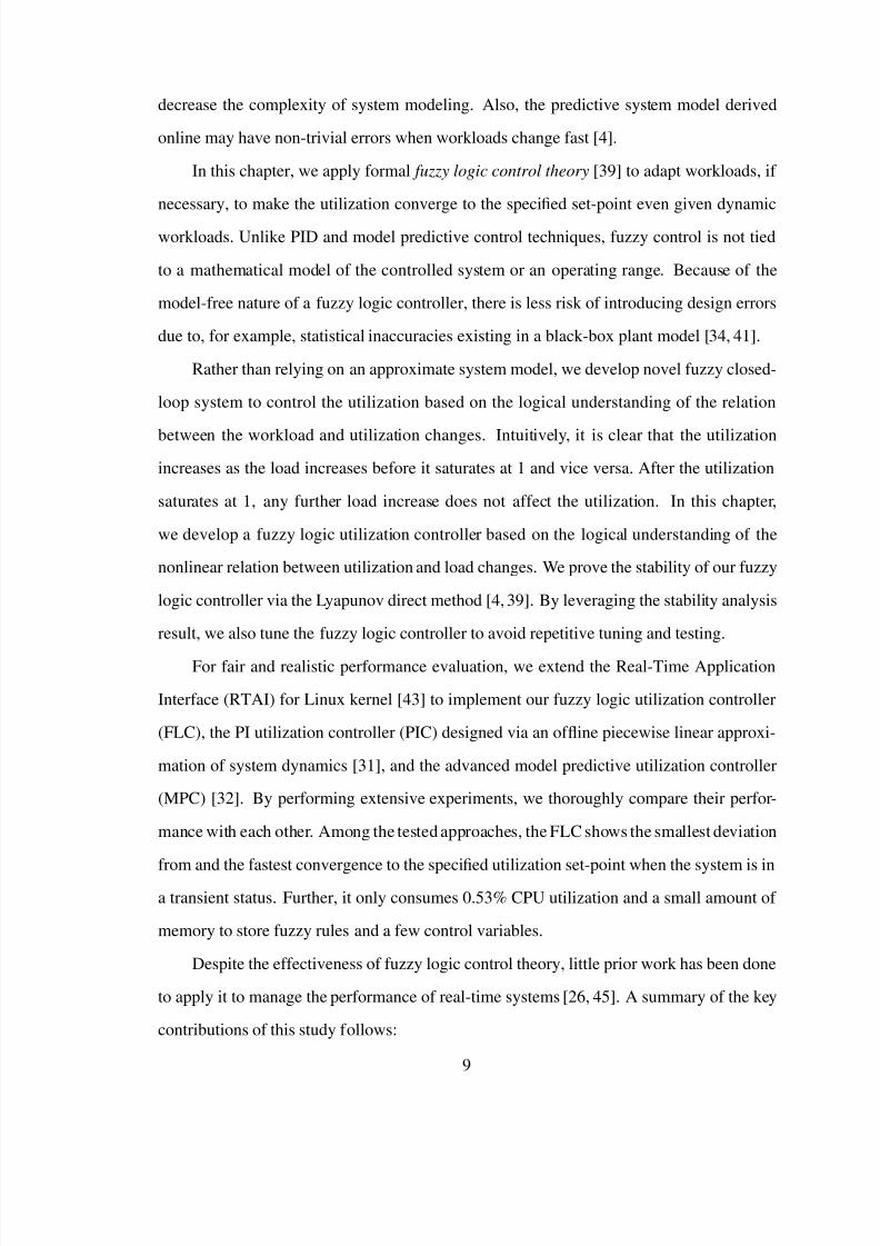
The high level structure of our closed-loop real-time system is shown in Figure 2.1.
The admission controller (AC) admits tasks based on the estimated utilization. An incom-ing task τc is admitted to the system only if total utilization U t = ∑ N
i=1 U i (for each task τi)
after admission does not exceed utilization set-point U s. Once admitted , periodic instances
of task τc are continuously executed by the scheduler. At the k th sampling point, current
system utilization u(k ) is provided to the controller which then computes necessary work-
load adjustment Δw(k ) to support U s. QoS manager enforces the workload adjustment by
12
7/31/2019 Mehmet Tez
http://slidepdf.com/reader/full/mehmet-tez 23/95
modifying periods of all active real-time tasks. A task’s period is always kept within the
bounds specified for that specific task. After the periods are adjusted, scheduler schedules
tasks using the adjusted periods. The period adjustment for a specific task is proportional
to Δw(k ) and its current period so that tasks with small periods receive small adjustments
and vice versa (Eq 2.5). In our system, tasks are notified via a signal after their periods are
updated.
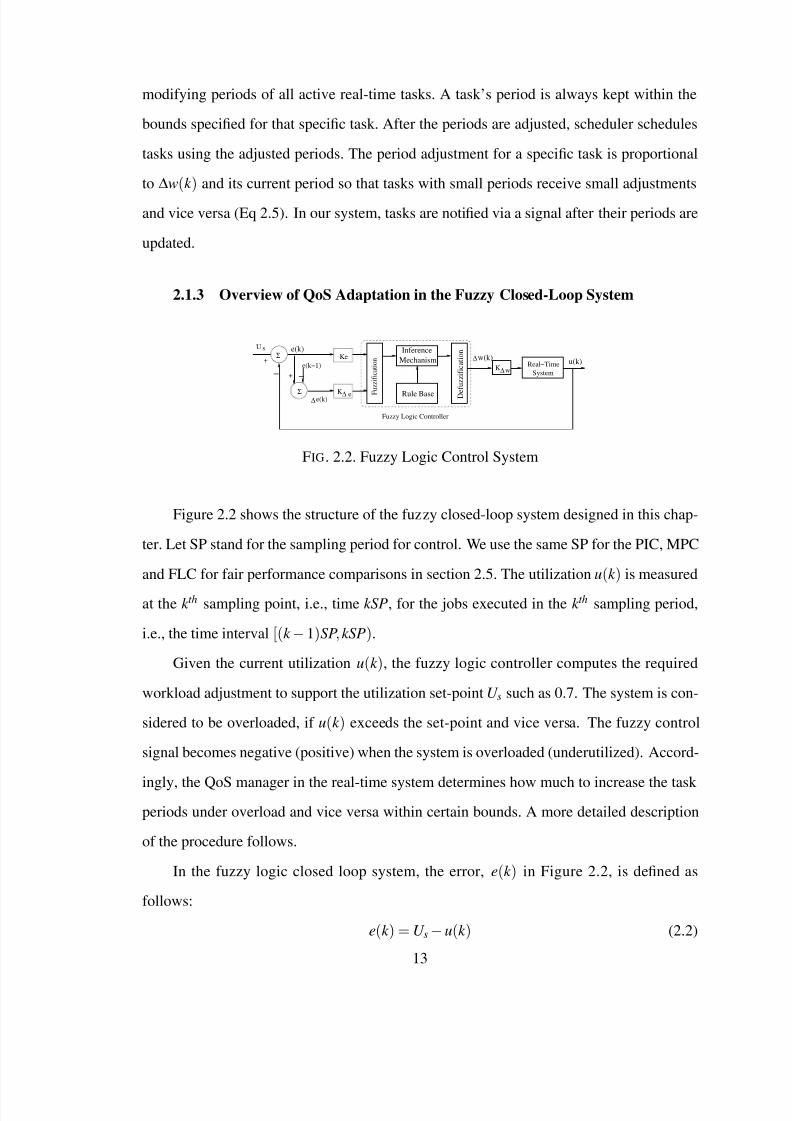
2.1.3 Overview of QoS Adaptation in the Fuzzy Closed-Loop System
sU
K
KeInference
Mechanism
Rule Base F
u z z i f i c a t i o n
D e
f u z z i f i c a t i o n
K w
Fuzzy Logic Controller
w(k)
Σ
Σ+
−
e(k)
+
e(k−1)
−
ΔΔ e
Δ
Δ
u(k)
SystemReal−Time
e(k)
FIG. 2.2. Fuzzy Logic Control System
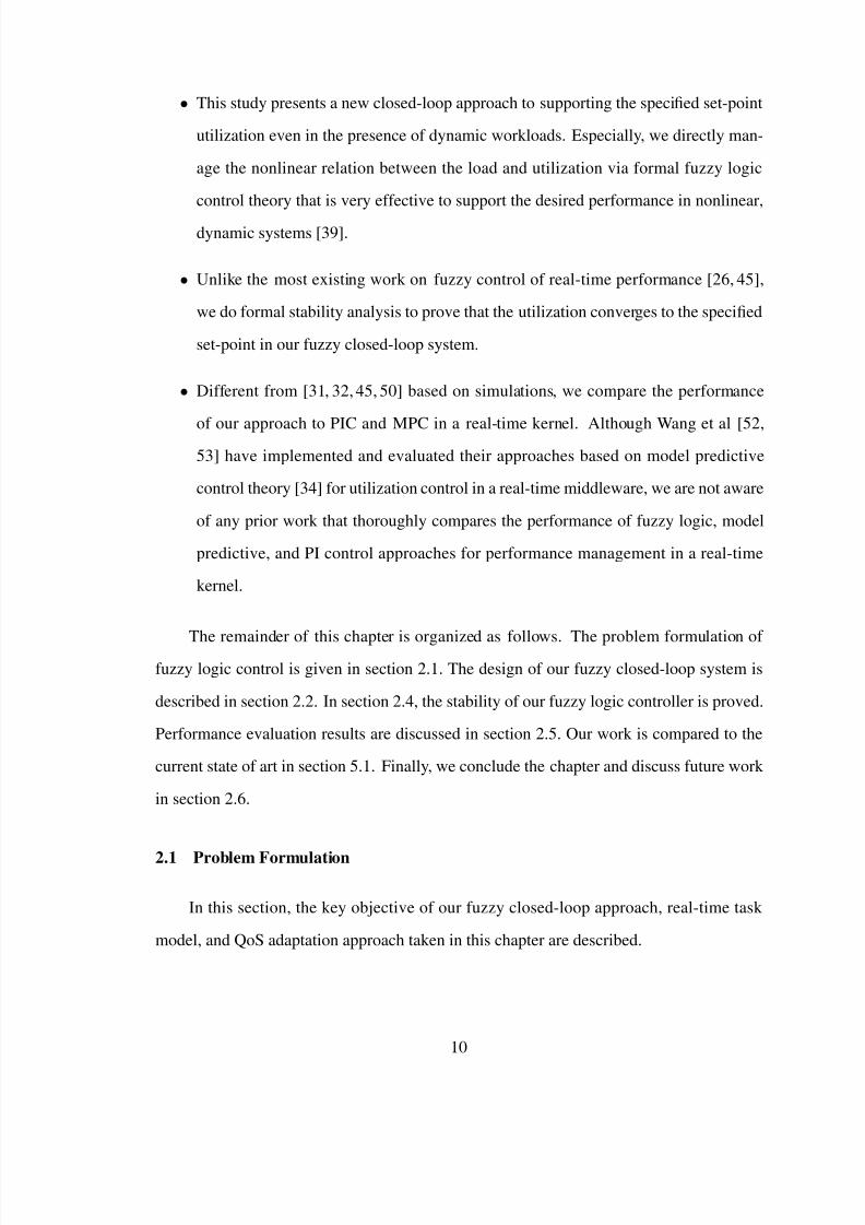
Figure 2.2 shows the structure of the fuzzy closed-loop system designed in this chap-
ter. Let SP stand for the sampling period for control. We use the same SP for the PIC, MPC
and FLC for fair performance comparisons in section 2.5. The utilization u(k ) is measured
at the k th sampling point, i.e., time kSP, for the jobs executed in the k th sampling period,
i.e., the time interval [(k − 1)SP, kSP).
Given the current utilization u(k ), the fuzzy logic controller computes the required
workload adjustment to support the utilization set-point U s such as 0.7. The system is con-
sidered to be overloaded, if u(k ) exceeds the set-point and vice versa. The fuzzy control
signal becomes negative (positive) when the system is overloaded (underutilized). Accord-
ingly, the QoS manager in the real-time system determines how much to increase the taskperiods under overload and vice versa within certain bounds. A more detailed description
of the procedure follows.
In the fuzzy logic closed loop system, the error, e(k ) in Figure 2.2, is defined as
follows:
e(k ) = U s − u(k ) (2.2)
13
7/31/2019 Mehmet Tez
http://slidepdf.com/reader/full/mehmet-tez 24/95
where U s is the utilization set-point. Also, we monitor the change in error:
Δe(k ) = e(k ) − e(k − 1) (2.3)
Based on the measured error and change in error, we directly manage the utilization
rather than relying on a black-box model that may involve non-trivial statistical errors, if
the load changes fast [34,41]. Based on e(k ) and Δe(k ), the FLC in Figure 2.2 computes
the required workload adjustment Δw(k ) for the next sampling period. The fuzzification
interface converts e(k ) and Δe(k ) to linguistic values such as negative small (NS) and pos-
itive small (PS). The inference mechanism looks up the knowledge base that has IF-THEN
rules to find the corresponding control signal. For example, an IF-THEN rule for utiliza-
tion control may state that if error is NS and change in error is PS, then the control signal
is NS. This rule dictates the QoS manager to reduce the load by a small amount. The de-
fuzzification1 interface converts the linguistic control signal to a crisp control signal Δw(k )
expressed as a real number such as -0.25. A detailed discussion of fuzzy control is given in
section 2.2.
Given the control signal Δw(k ), the QoS manager computes the period adaptation
factor F e(k + 1) for the next sampling period:
F e(k + 1) = F e(k ) · (1 − K ΔwΔw(k )) (2.4)
Note that the control signal in Eq 2.4, i.e. Δw(k ), is derived based on the potentially
nonlinear relationship between the load and utilization as described before. K Δw in Eq 2.4
is the control gain that needs to be tuned to support the stability of the closed-loop system.
(The stability of our closed-loop system is analyzed in section 2.4.)
As the control signal Δw(k ) is inverted in Eq 2.4, F e(k + 1) > F e(k ) and the periods
of real-time tasks will be increased to reduce the utilization if Δw(k ) < 0 due to overload
conditions and vice versa. If the system is overloaded at the k th sampling point, the period
1Fuzzification and defuzzification are standard terms in fuzzy logic control theory [39].
14
7/31/2019 Mehmet Tez
http://slidepdf.com/reader/full/mehmet-tez 25/95
of τi (1 ≤ i ≤ N − 1) is increased for the next sampling period; that is, T i(k + 1) > T i(k ).
Thus, the estimated load L is decreased by C iT i(k +1)−T i(k ) . Assuming the tasks are sorted in
descending order of the importance, QoS adaptation is applied to τi+1 and the next task(s)
until the sum of the estimated load adaptation becomes equal to K ΔwΔw(k ) or no task period
can be increased any further. Similarly, task periods are decreased according to the control
signal, if the system is underutilized.
Using the adaptation factor, the QoS manager in the real-time system computes:
T i(k + 1) = T i(k ) · F e(k + 1) (2.5)
for an arbitrary task τi in the real-time system and determines τi’s period for the (k + 1)th
sampling period, T i(k + 1), as follows:
T i(k + 1) =
⎧⎪⎪⎪⎨⎪⎪⎪⎩ T i(k + 1) if T i,min ≤ T i(k + 1) ≤ T i,max
T i,min if T i(k + 1) < T i,min
T i,max if T i(k + 1) > T i,max
(2.6)
Given Δw(k ), to support the utilization set-point, the period of every task in the system
is increased or decreased by the QoS manager and scheduler according to Eq 2.5 and Eq 2.6.
In this way, we avoid an unfair case in which one task’s period is increased (or decreased)
substantially within its minimum and maximum bounds, while others are not. Hence, the
required workload to support utilization set-point U s for the next period is calculated as:
w(k + 1) = w(k ) + K ΔwΔw(k ) (2.7)
From Eq 2.1 and Eq 2.6, we observe that it may not always be possible to adapt the
task period as much as indicated by K ΔwΔw(k ). This is especially a problem when the
system is currently overloaded and no task period can be extended anymore. In this case,
newly incoming tasks, if any, are rejected. Also, the least important tasks in the system are
temporarily suspended to fully enforce the control signal.
In this chapter, a certain load that lets the system to converge to the set-point is called
15
7/31/2019 Mehmet Tez
http://slidepdf.com/reader/full/mehmet-tez 26/95
the convergent load W . The difference between W and the current workload is formulated
as:
w(k ) = W − w(k ) (2.8)
In reality, W is unknown and it may vary in time depending on execution time estimation
errors. Thus, the purpose of fuzzy control is to adapt the workload based on e(k ) and Δe(k )
to support U s by minimizing |w(k )|, i.e., the absolute value of w(k ).
2.2 Fuzzy Logic Control
In this section, the key components of the FLC and control signal computation process
are described. Further, a detailed discussion of our rule-base design is given.
2.2.1 Fuzzy Logic Control Components for Control Signal Derivation
In this section, we describe standard fuzzy control terminologies [39] and describe
how to derive the control signal.
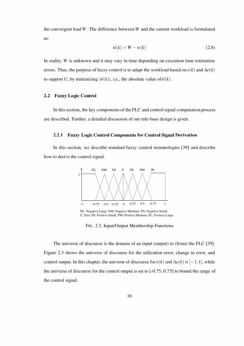
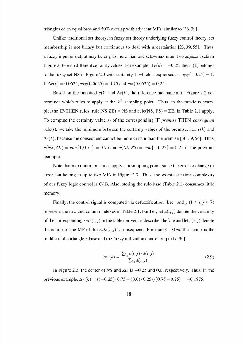
0
NL NM ZNS PS PM PL
NL: Negative Large, NM: Negative Medium, NS: Negative Small,Z: Zero, PS: Positive Small, PM: Positive Medium, PL: Positive Large
−0.75 −0.5 −0.25 0.25 0.5 0.75−1 1
1
FIG. 2.3. Input/Output Membership Functions
The universe of discourse is the domain of an input (output) to (from) the FLC [39].
Figure 2.3 shows the universe of discourse for the utilization error, change in error, and
control output. In this chapter, the universe of discourse for e(k ) and Δe(k ) is [−1, 1], while
the universe of discourse for the control output is set to [-0.75, 0.75] to bound the range of
the control signal.
16
7/31/2019 Mehmet Tez
http://slidepdf.com/reader/full/mehmet-tez 27/95
Δe(k )NL NM NS ZE PS PM PL
e(k )
NL NL NL NL NL NM NS ZENM NL NL NL NM NS ZE PSNS NL NL NM NS ZE PS PM
ZE NL NM NS ZE PS PM PLPS NM NS ZE PS PM PL PLPM NS ZE PS PM PL PL PLPL ZE PS PM PL PL PL PL
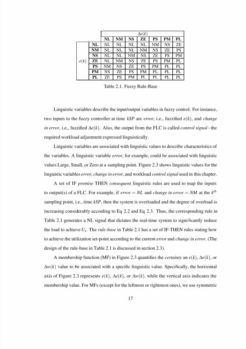
Table 2.1. Fuzzy Rule-Base
Linguistic variables describe the input/output variables in fuzzy control. For instance,
two inputs to the fuzzy controller at time kSP are error , i.e., fuzzified e(k ), and change
in error , i.e., fuzzified Δe(k ). Also, the output from the FLC is called control signal−the
required workload adjustment expressed linguistically.
Linguistic variables are associated with linguistic values to describe characteristics of
the variables. A linguistic variable error , for example, could be associated with linguistic
values Large, Small, or Zero at a sampling point. Figure 2.3 shows linguistic values for the
linguistic variables error , change in error , and workload control signal used in this chapter.
A set of IF premise THEN consequent linguistic rules are used to map the inputs
to output(s) of a FLC. For example, if error = NL and change in error = NM at the k th
sampling point, i.e., time kSP, then the system is overloaded and the degree of overload is
increasing considerably according to Eq 2.2 and Eq 2.3. Thus, the corresponding rule in
Table 2.1 generates a NL signal that dictates the real-time system to significantly reduce
the load to achieve U s. The rule-base in Table 2.1 has a set of IF-THEN rules stating how
to achieve the utilization set-point according to the current error and change in error . (The
design of the rule-base in Table 2.1 is discussed in section 2.3).
A membership function (MF) in Figure 2.3 quantifies the certainty an e(k ), Δe(k ), or
Δw(k ) value to be associated with a specific linguistic value. Specifically, the horizontal
axis of Figure 2.3 represents e(k ), Δe(k ), or Δw(k ), while the vertical axis indicates the
membership value. For MFs (except for the leftmost or rightmost ones), we use symmetric
17
7/31/2019 Mehmet Tez
http://slidepdf.com/reader/full/mehmet-tez 28/95
triangles of an equal base and 50% overlap with adjacent MFs, similar to [36, 39].
Unlike traditional set theory, in fuzzy set theory underlying fuzzy control theory, set
membership is not binary but continuous to deal with uncertainties [23, 39, 55]. Thus,
a fuzzy input or output may belong to more than one sets−maximum two adjacent sets in
Figure 2.3−with different certainty values. For example, if e(k ) = −0.25, then e(k ) belongs
to the fuzzy set NS in Figure 2.3 with certainty 1, which is expressed as: μ NS (−0.25) = 1.
If Δe(k ) = 0.0625, μ ZE (0.0625) = 0.75 and μPS (0.0625) = 0.25.
Based on the fuzzified e(k ) and Δe(k ), the inference mechanism in Figure 2.2 de-
termines which rules to apply at the k th sampling point. Thus, in the previous exam-
ple, the IF-THEN rules, rule(NS,ZE) = NS and rule(NS, PS) = ZE, in Table 2.1 apply.
To compute the certainty value(s) of the corresponding IF premise THEN consequent
rule(s), we take the minimum between the certainty values of the premise, i.e., e(k ) and
Δe(k ), because the consequent cannot be more certain than the premise [36,39, 54]. Thus,
μ( NS , ZE ) = min{1,0.75} = 0.75 and μ( NS , PS ) = min{1, 0.25} = 0.25 in the previous
example.
Note that maximum four rules apply at a sampling point, since the error or change in
error can belong to up to two MFs in Figure 2.3. Thus, the worst case time complexity
of our fuzzy logic control is O(1). Also, storing the rule-base (Table 2.1) consumes little
memory.
Finally, the control signal is computed via defuzzification. Let i and j (1 ≤ i, j ≤ 7)
represent the row and column indexes in Table 2.1. Further, let μ(i, j) denote the certainty
of the corresponding rule(i, j) in the table derived as described before and let c(i, j) denote
the center of the MF of the rule(i, j)’s consequent. For triangle MFs, the center is the
middle of the triangle’s base and the fuzzy utilization control output is [39]:
Δw(k ) =∑i, j c(i, j) ·μ(i, j)
∑i, jμ(i, j)(2.9)
In Figure 2.3, the center of NS and ZE is −0.25 and 0.0, respectively. Thus, in the
previous example, Δw(k ) = ((−0.25) · 0.75 + (0.0) · 0.25)/(0.75 + 0.25) = −0.1875.
18
7/31/2019 Mehmet Tez
http://slidepdf.com/reader/full/mehmet-tez 29/95
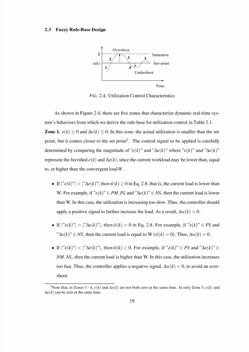
2.3 Fuzzy Rule-Base Design
1
1
2 3 5
4u(k)
Time
Overshoot
Undershoot
Set−
point
Saturation
FIG. 2.4. Utilization Control Characteristics
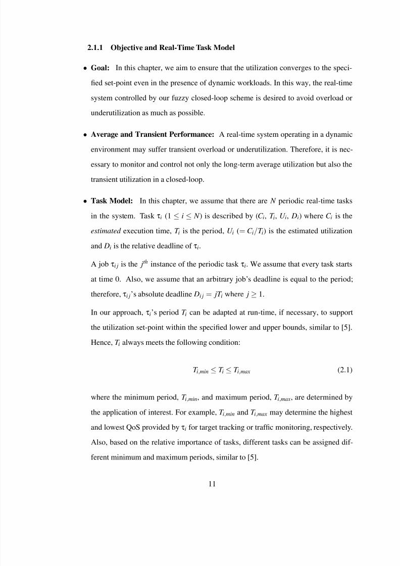
As shown in Figure 2.4, there are five zones that characterize dynamic real-time sys-
tem’s behaviors from which we derive the rule-base for utilization control in Table 2.1.Zone 1. e(k ) ≥ 0 and Δe(k ) ≤ 0: In this zone, the actual utilization is smaller than the set
point, but it comes closer to the set point2. The control signal to be applied is carefully
determined by comparing the magnitude of ”e(k )” and ”Δe(k )” where ”e(k )” and ”Δe(k )”
represent the fuzzified e(k ) and Δe(k ), since the current workload may be lower than, equal
to, or higher than the convergent load W .
• If |”e(k )”| > |”Δe(k )”| then w(k ) ≥ 0 in Eq. 2.8; that is, the current load is lower thanW. For example, if ”e(k )” ∈ PM , PL and ”Δe(k )” ∈ NS , then the current load is lower
than W. In this case, the utilization is increasing too slow. Thus, the controller should
apply a positive signal to further increase the load. As a result, Δw(k ) > 0.
• If |”e(k )”| = |”Δe(k )”|, then w(k ) = 0 in Eq. 2.8. For example, if ”e(k )” ∈ PS and
”Δe(k )” ∈ NS , then the current load is equal to W ( w(k ) = 0). Thus, Δw(k ) = 0.
• If |”e(k )”| < |”Δe(k )”|, then w(k ) < 0. For example, if ”e(k )” ∈ PS and ”Δe(k )” ∈
NM , NL, then the current load is higher than W. In this case, the utilization increases
too fast. Thus, the controller applies a negative signal, Δw(k ) < 0, to avoid an over-
shoot.
2Note that, in Zones 1−4, e(k ) and Δe(k ) are not both zero at the same time. In only Zone 5, e(k ) andΔe(k ) can be zero at the same time.
19

7/31/2019 Mehmet Tez
http://slidepdf.com/reader/full/mehmet-tez 30/95
Zone 2. e(k ) < 0 and Δe(k ) ≤ 0: In this zone, the utilization is higher than the set-point and
it is further increasing. It indicates that the current load is higher than W; that is, w(k ) < 0.
Hence, the controller applies Δw(k ) < 0 to reverse the current trend.
Zone 3. e(k ) ≤ 0 and Δe(k ) ≥ 0: In this zone, the utilization is higher than the set point,
but it comes closer to the set point. The control signal should be carefully determined
by comparing the magnitude of ”e(k )” and ”Δe(k )” as the current workload value may be
lower than, equal to, or higher than W value.
• If |”e(k )”| > |”Δe(k )”|,then w(k ) < 0. For example, if ”e(k )” ∈ NM , NL and”Δe(k )” ∈
PS then the current load is higher than W; that is, w(k ) < 0. As the utilization is de-
creasing too slow, the controller should apply a negative signal to further reduce the
load.
• If |”e(k )”| = |”Δe(k )”|, then w(k ) = 0. For example, if ”e(k )” ∈ NS and”Δe(k )” ∈ PS ,
then the current load is equal to W. Thus, Δw(k ) = 0.
• If |”e(k )”| < |”Δe(k )”|, then w(k ) > 0. For example, if ”e(k )” ∈ NS and ”Δe(k )” ∈
PM , PL, then the current load is lower than W. The utilization is decreasing too fast
in this case. Thus, the controller should apply a positive signal to increase the load
to support U s, i.e., Δw(k ) > 0.
Zone 4. e(k ) > 0 and Δe(k ) ≥ 0: In this zone, the actual utilization is lower than the set-
point and it is further decreasing. It indicates that the current workload is lower than W,
i.e., w(k ) > 0. Thus, Δw(k ) > 0.
Zone 5. |e(k )| ≤ ε and |Δe(k )| ≤ ε where ε is a small predefined real number: In this case,
the real-time system is in the steady state. Δw(k ) = 0, as the current workload is equal to W,
i.e., w(k ) = 0. In section 2.4, we prove that the fuzzy closed-loop system asymptotically
convergences to the ε neighborhood of the set-point.
To summarize, the relationship between the control output and inputs in Table 2.1 can
be formulated in linguistic terms:
”Δw(k )” = ”e(k )” + ”Δe(k )”
20

7/31/2019 Mehmet Tez
http://slidepdf.com/reader/full/mehmet-tez 31/95
The linguistic value of ” w(k )” can be determined from these five zones. Our fuzzy
logic rule-base containing the five zones implies the following linguistic equation:
” w(k )” = ”Δw(k )” (2.10)
which can be validated by inspecting the rule base and explanation of the fuzzy control
actions in the five zones. In our rule-base, the sign of Δw(k ) is equal to the sign of w(k ).
This is because, in each zone, the sign of Δw(k ) is determined based on the sign of w(k ) as
discussed earlier in this section. Also, the control signal’s magnitude is proportional to the
difference between W and current load.
2.4 Stability Analysis and Tuning
In this section, the stability of the closed-loop system is analyzed and the control gains,
i.e., Ke, K Δe and K Δw in Figure 2.2, are tuned.
2.4.1 Stability Analysis
In this chapter, we prove the stability of our fuzzy closed-loop system via the Lya-
punov Direct Method [4,39].
Theorem 2.4.1 Lyapunov Direct Method [4, 39]. If the following conditions are true for
an arbitrary function V ( x(k )) : Rn → R where n ≥ 1 ,
V ( x(k )) = 0, i f x(k ) = 0
V ( x(k )) > 0, i f x(k ) ∈ Rn − {0}
V ( x(k + 1)) −V ( x(k )) < 0
then V ( x(k )) is a Lyapunov candidate function (LCF) in some region D ∈ Rn which con-
tains the origin. V ( x(k )) guarantees the asymptotic stability around zero. (Any nonzero
equilibrium point can be transformed to the origin via change of variables.)
21

7/31/2019 Mehmet Tez
http://slidepdf.com/reader/full/mehmet-tez 32/95
We apply Theorem 2.4.1 to prove the stability of our closed loop fuzzy control system.
Specifically, we choose the LCF function as:
V (w(k + 1)) = w 2(k + 1). (2.11)
Theorem 2.4.2 If the V (w(k + 1)) has the LCF function properties, then the closed loop
fuzzy control system is asymptotically stable around the set point.
Proof The LCF function has the following properties:
V (w(k + 1)) = 0, i f w(k + 1) = 0
V (w(k + 1)) > 0, i f w(k + 1) ∈ R − {0}
To meet all the requirements to be a LCF, this function should also have the following
property:
V (w(k + 1)) −V (w(k )) = w 2(k + 1) − w 2(k ) < 0 (2.12)
Using Eq. 2.7 and Eq. 2.8, we get:
w(k + 1) = W − w(k + 1)
= W − [w(k ) + K ΔwΔw(k )]
= W − w(k ) − K ΔwΔw(k )
= w(k ) − K ΔwΔw(k ) (2.13)
From Eq. 2.12 and Eq. 2.13, we derive that:
V (w(k + 1)) −V (w(k )) = [w(k ) − K ΔwΔw(k )]2 − w 2(k )
= K ΔwΔw(k ) [K ΔwΔw(k ) − 2 w(k )] < 0
22
7/31/2019 Mehmet Tez
http://slidepdf.com/reader/full/mehmet-tez 33/95
To ensure this inequality, the following constraints should be met:
sign(w(k )) = sign(Δw(k )) (2.14)
|Δw(k )| <2
K Δw
|w(k )| (2.15)
The first constraint (Eq. 2.14) is met, since “ w(k )” = “Δw(k )” (Eq. 2.10). As W and thus
w(k ) are not measurable directly, we can change the second constraint (Eq. 2.15) by replac-
ing w(k ) with a small positive real number ε:
|Δw(k )| <
2
K Δw ε, ε ∈ R+
(2.16)
If this inequality holds for w(k ) ≥ ε, then w(k ) will asymptotically converge to an ε neigh-
borhood of the convergent load. Specifically, 0 < K Δw < 2/0.75 sinceΔw(k ) = [−0.75, 0.75]
as discussed in section 2.2.1. This concludes the proof of the stability of our fuzzy closed-
loop system.
2.4.2 Fuzzy Controller Tuning
We need to tune Ke, K Δe and K Δw in Figure 2.2 for good performance. To support the
stability of the fuzzy closed-loop system, we must meet the condition that 0 < K Δw < 2.6
as derived in Theorem 2.4.2. K Δw of a larger value reduces the settling time, but it may
cause a higher overshoot. In this chapter, we set K Δw = 1 to balance the settling time and
overshoot, while focusing slightly more on reducing potential overshoots. Generally, K Δw
has the largest effect on the system performance, because it directly affects the stability in
addition to the settling time and overshoot. On the other hand, K e and K Δe do not directly
affect the stability according to Theorem 2.4.2. In this chapter, K e is set to 1 so that the
controller can utilize the whole rule base for the error input. On the other hand, we set
K Δe = 0.1 to damp potentially jittery change-in-error values. Generally, a large K Δe reduces
the settling time, but increases the overshoot.
23

7/31/2019 Mehmet Tez
http://slidepdf.com/reader/full/mehmet-tez 34/95
2.5 Performance Evaluation
In this section, a description of the experimental set-up for evaluating the FLC, MPC,
and PIC is given. Also, the performance evaluation results are discussed.
2.5.1 Experimental Settings
We have implemented the FLC, MPC, and PIC in the RTAI 3.6 [43]. The Linux
kernel version 2.6.22 is installed on a 2.3GHz Pentium 4 machine with 1 GB RAM. We
have modified the real-time scheduler provided by RTAI to collect performance statistics
and implement the controllers. We have implemented and tuned the PIC as described in
[31]. Also, we have implemented the MPC described in [32] with the prediction horizon
P = 2 and control horizon M = 1.
Name Value
Set-point (U s) 0.7Sampling period (SP) 1 secondAlgorithm EDFDeadline semantics FirmEstimated execution time [50μs, 100μs]Task period [300μs, 4ms]
Run length 300 secondsRuns per load profile 10Load profiles Ramp, Step, Sawtooth, TASKx6 & Step5-Random
Table 2.2. System parameters
As described in section 2.1, all the controllers output the period adaptation factor F e
in Eq. 2.4 used to adapt the periods of real-time tasks in the system. Each controller is
invoked at every sampling point to compute the required workload adjustment to support
the utilization set-point U s. In this chapter, SP is set to 1s and U s is set to 0.7 as shown in
Table 2.2. Tasks are scheduled according to the EDF (Earliest Deadline First) algorithm.
The deadlines are firm; that is, a task instance is canceled as soon as it misses its deadline.
For performance evaluation, we generate periodic real-time tasks. As shown in Ta-
ble 2.2, the estimated execution time of a task to be generated is uniformly selected in the
24

7/31/2019 Mehmet Tez
http://slidepdf.com/reader/full/mehmet-tez 35/95
range of [50μs, 100μs]. Further, the period of the task is uniformly selected in the range
of [300μs, 4ms]. Each job is associated with an actual execution time: AET i j = α · EET i j
where EET i j is the estimated execution time of job τi j in the system and α is the execu-
tion time factor , similar to [31,32]. In this way, fair performance comparisons are possible
among the PIC, MPC, and FLC.
0.3
5
0 50 100 150 200 250 300
α
Time (secs)
(a) Ramp
0.3
0.6
0 50 100 150 200 250 300
α
Time (secs)
(b) Step
0.2
0.60.8
1
2
3
4
5
0 50 100 150 200 250 300
α
Time (secs)
(c) Sawtooth
FIG. 2.5. Tested Workloads
The worst case execution time of τi j is equal to the maximum of the possible AET i j
values that are varied by α. Note that the EDF scheduler and controllers (i.e., PIC, MPC,
and FLC) are aware of neither the actual nor the worst case execution times, because α
is unknown to them. When α > 1, they may underestimate execution times. As a result,
they may overload the system, missing deadlines. On the other hand, when α < 1, theymay underutilize the system. Thus, we evaluate how closely the FLC, MPC, and PIC can
support U s when α varies. To this end, we have created several different experimental load
profiles summarized in Table 2.2. For each profile, 10 runs are executed and the average of
the 10 runs is reported. Each run executes a random task set for 300s.
In Figure 2.5, the ramp load continuously increases as α increases from 0.3 to 5 over
25
7/31/2019 Mehmet Tez
http://slidepdf.com/reader/full/mehmet-tez 36/95
300s. The step load tests the robustness of the controller given a sudden load increase and
decrease in a step manner. There are five variations of the step load. Each of them starts
with α = 1 and an initial load of 60%. At 100s, α is increased to 2, 3, 4, and 5 for Step-2,
Step-3, Step-4, and Step-5, respectively. Further, α is decreased to 0.3 at 200s.
The ramp and step workloads are widely used to evaluate control performance [16,
31, 32, 41]. We use them for fair performance comparisons between the fuzzy controller
and the PIC [31] and MPC [32]. In addition, we consider the sawtooth load that concate-
nates multiple ramp loads to stress the real-time system by increasing or decreasing α at a
constant rate.
At the beginning of an experimental run, each task τi runs at its minimum period T i,min.
To satisfy Eq 2.1, the maximum period of a task τi is:
T i,max = xT i,min (2.17)
For the set of experiments presented in sections 2.5.3 - 2.5.5, x = 4. For the experiments
presented in section 2.5.6, we fix α to 2 and randomly choose x in Eq 2.17 in the range
[2, 6] for each task, but we increase the number of tasks by six times. This workload is
called TASKx6 workload in this chapter. In section 2.5.7, we use a different workload
called Step5-Random where α is increased to 5 at 100s and x is randomly selected in the
range [2, 6] to further evaluate FLC, MPC, and PIC in dynamic environments. In our ex-
periments reported in this chapter, approximately 340,000 − 1, 500, 000 jobs, i.e., periodic
task instances, are generated for a 300s run depending on the specific workload.
2.5.2 Experiment Results
In this section, the performance evaluation results of the FLC, MPC, and PIC for
the ramp, step, and sawtooth workloads are discussed. In our experiments, all the tested
approaches admitted all real-time tasks, because the estimated total utilization computed
based on the estimated execution times is smaller than 1−the schedulable utilization bound
of the EDF scheduling algorithm [29]. Also, no task was suspended in this chapter.
26

7/31/2019 Mehmet Tez
http://slidepdf.com/reader/full/mehmet-tez 37/95
In our experiments, all the tested closed-loop approaches successfully supported the
average utilization set-point for most of the experiments by adapting task periods according
to the feedback control signal as directed in Eq 2.6. Therefore, we focus on the transient
performance results in the following. Note that it is critical to manage not only the long-
term average but also transient performance in a mission-critical real-time system.
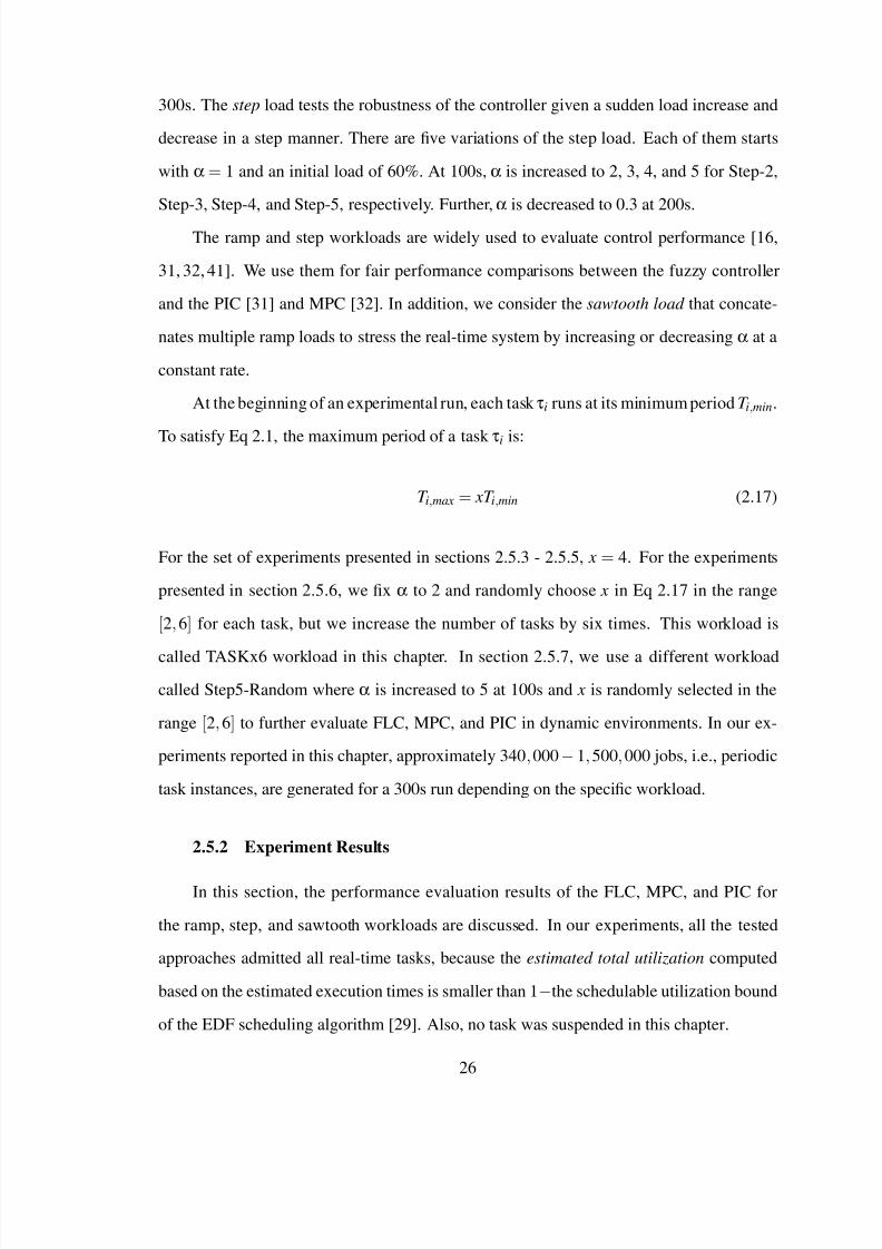
2.5.3 Ramp Workload
The results for the ramp load are given in Figure 2.6. The PIC has non-zero steady
state errors that do not decay until the end of the experiment at 300s as shown in Figure 2.6.
Thus, we observe that the PIC clearly fails to support the set-point, which is important as
the set-point support not only provides a safety-margin for bursts but it also allows for
resource sharing possibly between non-real-time tasks and real-time tasks. In contrast, the
MPC cancels an initial utilization overshoot. MPC’s settling time is approximately 40s. As
shown in Figure 2.6, the FLC’s settling time is only about 10s. Also, it shows the smallest
overshoot. From these results, we observe that the FLC achieves the best performance
among the tested approaches for the ramp load.
For the ramp workload, all the tested approaches meet all the task deadlines as the
α value increases only gradually. Although the PIC meets all the deadlines, its utilization
does not converge to the set-point and it is higher than the set-point as discussed before.
Thus, the PIC leaves less CPU cycles available to non-real-time tasks (if any). Also, it is
possible for the PIC to miss deadlines, if a higher utilization set-point is used.
To further analyze the set-point tracking performance, we define the aggregated error
E agg:
E agg = 1n n
∑k =1(U s − u(k ))2 (2.18)
where n is the number of the sampling points in one experimental run. For the ramp work-
loads, the FLC reduces E agg by 56% and 74% compared to the MPC and PIC. Specifically,
E agg = 0.0056 for the FLC, while E agg = 0.0127 and E agg = 0.0215 for MPC and PIC, re-
spectively. Overall, the FLC supports the smallest deviations from the set-point and shortest
27
7/31/2019 Mehmet Tez
http://slidepdf.com/reader/full/mehmet-tez 38/95
0.6
0.65
0.7
0.75
0.8
0 50 100 150 200 250 300
U t i l i z a t i o n
Time (sec)
MPCPICFLC
FIG. 2.6. Transient Utilization for the Ramp Load
settling times for the ramp load.
For all the tested workloads, the FLC, MPC, and PIC adjust the task periods in a sim-
ilar fashion. The average period adaptations achieved by them are almost equal. However,
the transient period adaptation of the FLC is faster than the others. This result shows the
higher adaptivity of the FLC to dynamic workloads.
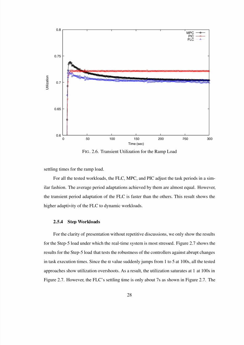
2.5.4 Step Workloads
For the clarity of presentation without repetitive discussions, we only show the results
for the Step-5 load under which the real-time system is most stressed. Figure 2.7 shows the
results for the Step-5 load that tests the robustness of the controllers against abrupt changes
in task execution times. Since the α value suddenly jumps from 1 to 5 at 100s, all the tested
approaches show utilization overshoots. As a result, the utilization saturates at 1 at 100s in
Figure 2.7. However, the FLC’s settling time is only about 7s as shown in Figure 2.7. The
28
7/31/2019 Mehmet Tez
http://slidepdf.com/reader/full/mehmet-tez 39/95
0
0.2
0.4
0.6
0.8
1
0 50 100 150 200 250 300
U t i l i z a t i o n
Time (sec)
MPCPICFLC
FIG. 2.7. Transient Utilization for the Step-5 Load
settling time of the MPC, 55s, is approximately eight times longer than the FLC’s.
Further, the FLC achieves the smallest E agg. Specifically, E agg = 0.0611, 0.0714, and
0.1227 for the FLC, MPC, and PIC, respectively. Thus, the FLC reduces E agg by ap-
proximately 50% compared to the PIC. Furthermore, it reduces E agg by more than 14%
compared to the MPC with the less complex controller design than the MPC.
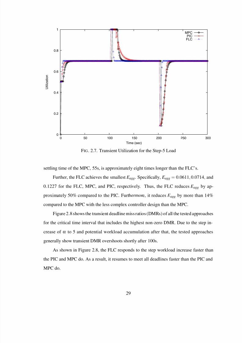
Figure 2.8 shows the transient deadline miss ratios (DMRs) of all the tested approaches
for the critical time interval that includes the highest non-zero DMR. Due to the step in-
crease of α to 5 and potential workload accumulation after that, the tested approaches
generally show transient DMR overshoots shortly after 100s.
As shown in Figure 2.8, the FLC responds to the step workload increase faster than
the PIC and MPC do. As a result, it resumes to meet all deadlines faster than the PIC and
MPC do.
29
7/31/2019 Mehmet Tez
http://slidepdf.com/reader/full/mehmet-tez 40/95
0
0.2
0.4
0.6
0.8
1
95 100 105 110 115 120 125
D e a d l i n e M i s s R a t i o
Time (sec)
MPCPICFLC
FIG. 2.8. Transient Deadline Miss Ratio for the Step-5 Load
2.5.5 Sawtooth Workload
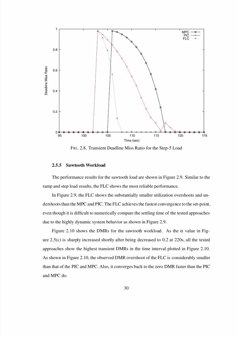
The performance results for the sawtooth load are shown in Figure 2.9. Similar to the
ramp and step load results, the FLC shows the most reliable performance.
In Figure 2.9, the FLC shows the substantially smaller utilization overshoots and un-
dershoots than the MPC and PIC. The FLC achieves the fastest convergence to the set-point,
even though it is dif ficult to numerically compare the settling time of the tested approaches
due to the highly dynamic system behavior as shown in Figure 2.9.
Figure 2.10 shows the DMRs for the sawtooth workload. As the α value in Fig-
ure 2.5(c) is sharply increased shortly after being decreased to 0.2 at 220s, all the tested
approaches show the highest transient DMRs in the time interval plotted in Figure 2.10.
As shown in Figure 2.10, the observed DMR overshoot of the FLC is considerably smaller
than that of the PIC and MPC. Also, it converges back to the zero DMR faster than the PIC
and MPC do.
30
7/31/2019 Mehmet Tez
http://slidepdf.com/reader/full/mehmet-tez 41/95
0.3
0.4
0.5
0.6
0.7
0.8
0.9
1
0 50 100 150 200 250 300
U t i l i z a t i o n
Time (sec)
MPCPICFLC
FIG. 2.9. Transient Utilization for the Sawtooth Load
0
0.1
0.2
0.3
0.4
0.5
0.6
0.7
220 225 230 235 240
D e a d l i n e M i s s R a t i o
Time (sec)
MPCPICFLC
FIG. 2.10. Transient Deadline Miss Ratio for the Sawtooth Load
31
7/31/2019 Mehmet Tez
http://slidepdf.com/reader/full/mehmet-tez 42/95
Moreover, E agg = 0.0568,0.073, and 0.0994 for the FLC, MPC, and PIC. Thus, the
FLC reduces E agg by more than 22% and 42% compared to the MPC and PIC, respectively.
These results demonstrate the effectiveness and robustness of fuzzy control.
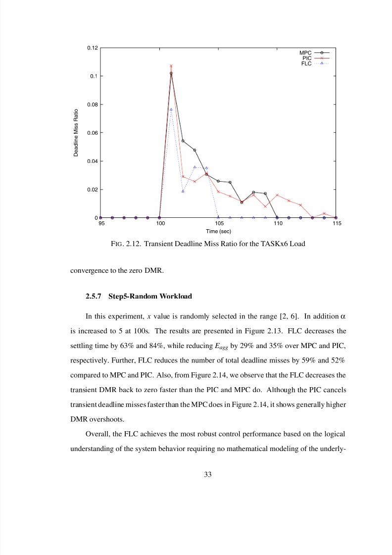
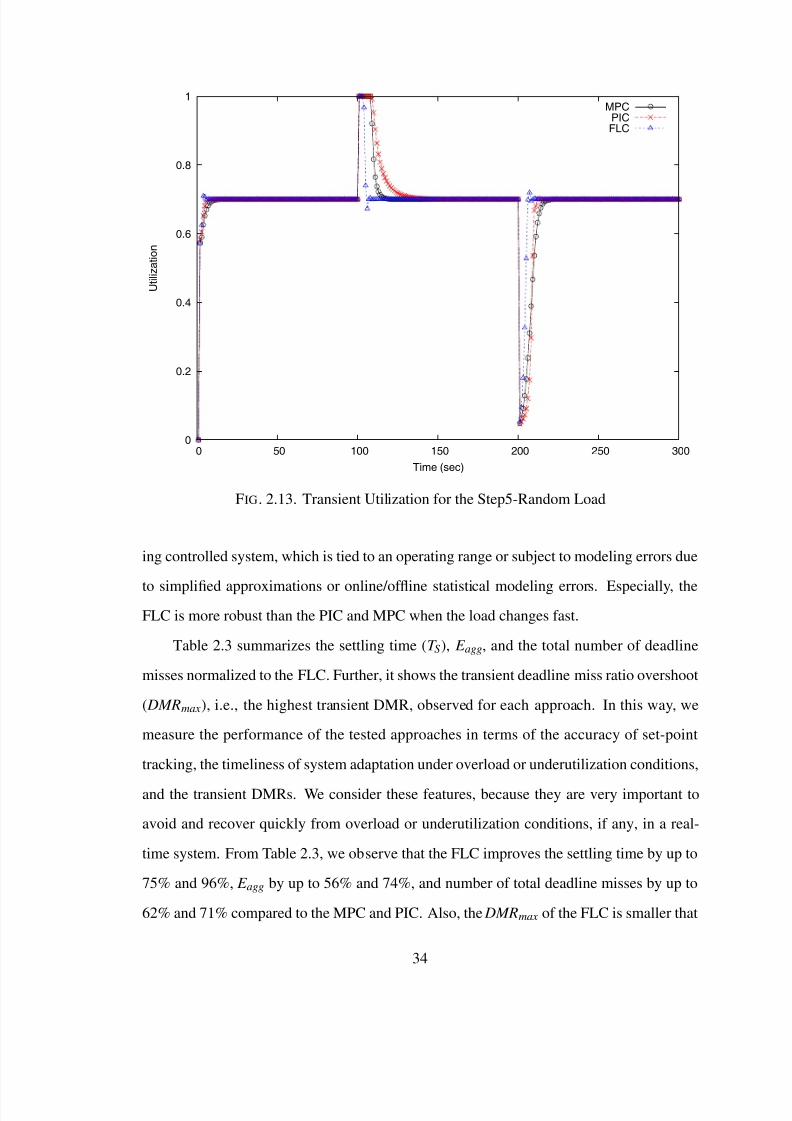
2.5.6 TASKx6 Workload
0.5
0.6
0.7
0.8
0.9
1
0 50 100 150 200 250 300
U t i l i z a t i o n
Time (sec)
MPCPICFLC
FIG. 2.11. Transient Utilization for the TASKx6 Load
In the TASKx6 workload, we abruptly increase the number of real-time tasks in the
system rather than increasing the α value, which is kept fixed at α= 2. The number of tasks
in the system is increased by 6 times at time 100s. As a result, the load increases from 70%to 420%. Also, the x value in Eq. 2.17 is randomly selected within the range [2,6] for each
task. As shown in Figure 2.11, FLC improves the settling time by 29% and 72% compared
to MPC and PIC, respectively. Also, it decreases E agg by 17% and 32%, while reducing
the total number of deadline misses by 50% and 46% over MPC and PIC, respectively. For
these reasons, in Figure 2.12, the FLC achieves the smallest DMR overshoot and fastest
32
7/31/2019 Mehmet Tez
http://slidepdf.com/reader/full/mehmet-tez 43/95
0
0.02
0.04
0.06
0.08
0.1
0.12
95 100 105 110 115
D e a d l i n e M i s s R a t i o
Time (sec)
MPCPICFLC
FIG. 2.12. Transient Deadline Miss Ratio for the TASKx6 Load
convergence to the zero DMR.
2.5.7 Step5-Random Workload
In this experiment, x value is randomly selected in the range [2, 6]. In addition α
is increased to 5 at 100s. The results are presented in Figure 2.13. FLC decreases the
settling time by 63% and 84%, while reducing E agg by 29% and 35% over MPC and PIC,
respectively. Further, FLC reduces the number of total deadline misses by 59% and 52%
compared to MPC and PIC. Also, from Figure 2.14, we observe that the FLC decreases the
transient DMR back to zero faster than the PIC and MPC do. Although the PIC cancels
transient deadline misses faster than the MPC does in Figure 2.14, it shows generally higher
DMR overshoots.
Overall, the FLC achieves the most robust control performance based on the logical
understanding of the system behavior requiring no mathematical modeling of the underly-
33
7/31/2019 Mehmet Tez
http://slidepdf.com/reader/full/mehmet-tez 44/95
0
0.2
0.4
0.6
0.8
1
0 50 100 150 200 250 300
U t i l i z a t i o n
Time (sec)
MPCPICFLC
FIG. 2.13. Transient Utilization for the Step5-Random Load
ing controlled system, which is tied to an operating range or subject to modeling errors due
to simplified approximations or online/of fline statistical modeling errors. Especially, theFLC is more robust than the PIC and MPC when the load changes fast.
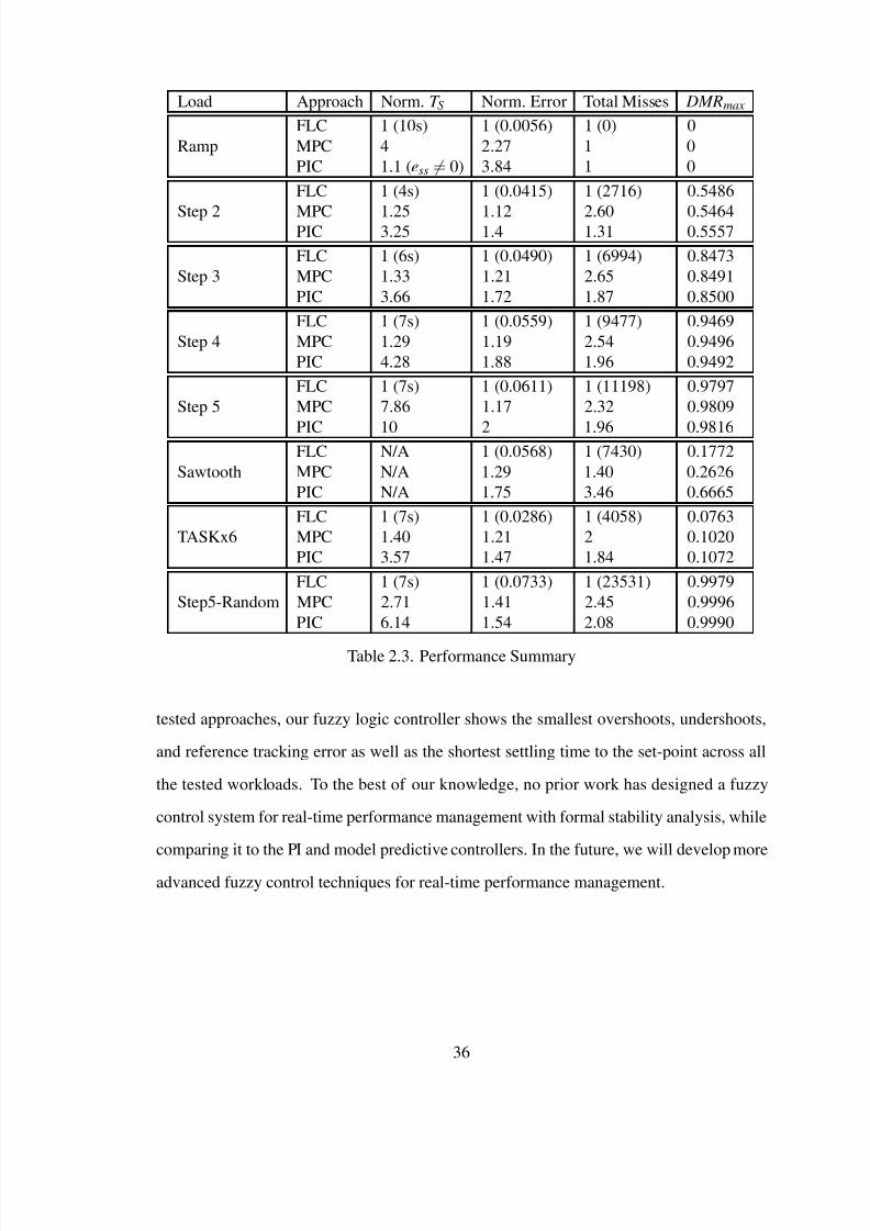
Table 2.3 summarizes the settling time (T S ), E agg, and the total number of deadline
misses normalized to the FLC. Further, it shows the transient deadline miss ratio overshoot
( DMRmax), i.e., the highest transient DMR, observed for each approach. In this way, we
measure the performance of the tested approaches in terms of the accuracy of set-point
tracking, the timeliness of system adaptation under overload or underutilization conditions,
and the transient DMRs. We consider these features, because they are very important to
avoid and recover quickly from overload or underutilization conditions, if any, in a real-
time system. From Table 2.3, we observe that the FLC improves the settling time by up to
75% and 96%, E agg by up to 56% and 74%, and number of total deadline misses by up to
62% and 71% compared to the MPC and PIC. Also, the DMRmax of the FLC is smaller that
34

7/31/2019 Mehmet Tez
http://slidepdf.com/reader/full/mehmet-tez 45/95
0
0.2
0.4
0.6
0.8
1
95 100 105 110 115 120 125
D e a d l i n e M i s s R a t i o
Time (sec)
MPCPICFLC
FIG. 2.14. Transient Deadline Miss Ratio for the Step5-Random Load
that of the PIC and MPC except for the Ramp and Step 2 workloads.
Finally, Table 2.4 shows overhead of the tested controllers. All the controllers are
lightweight and consume less than 1% CPU utilization for the sampling period of 1s. The
PIC has the lowest overhead while the MPC has the highest overhead due to the complexity.
The FLC consumes approximately 0.5% CPU utilization and a small amount of memory.
2.6 Summary
In a number of real-time applications such as target tracking and traf fic control, it is
challenging to support the desired real-time performance. To closely support the specified
utilization set-point in the presence of dynamic workloads and system behaviors, we de-
sign a fuzzy closed-loop system, while mathematically proving the stability of the fuzzy
closed-loop system. Also, extensive experiments are performed to thoroughly evaluate the
fuzzy, PI [31], and model predictive [32] controllers in a real-time kernel. Among the
35
7/31/2019 Mehmet Tez
http://slidepdf.com/reader/full/mehmet-tez 46/95
Load Approach Norm. T S Norm. Error Total Misses DMRmax
RampFLC 1 (10s) 1 (0.0056) 1 (0) 0MPC 4 2.27 1 0PIC 1.1 (ess = 0) 3.84 1 0
FLC 1 (4s) 1 (0.0415) 1 (2716) 0.5486
Step 2 MPC 1.25 1.12 2.60 0.5464PIC 3.25 1.4 1.31 0.5557
FLC 1 (6s) 1 (0.0490) 1 (6994) 0.8473Step 3 MPC 1.33 1.21 2.65 0.8491
PIC 3.66 1.72 1.87 0.8500
FLC 1 (7s) 1 (0.0559) 1 (9477) 0.9469Step 4 MPC 1.29 1.19 2.54 0.9496
PIC 4.28 1.88 1.96 0.9492
FLC 1 (7s) 1 (0.0611) 1 (11198) 0.9797Step 5 MPC 7.86 1.17 2.32 0.9809
PIC 10 2 1.96 0.9816
SawtoothFLC N/A 1 (0.0568) 1 (7430) 0.1772MPC N/A 1.29 1.40 0.2626PIC N/A 1.75 3.46 0.6665
FLC 1 (7s) 1 (0.0286) 1 (4058) 0.0763TASKx6 MPC 1.40 1.21 2 0.1020
PIC 3.57 1.47 1.84 0.1072
FLC 1 (7s) 1 (0.0733) 1 (23531) 0.9979Step5-Random MPC 2.71 1.41 2.45 0.9996
PIC 6.14 1.54 2.08 0.9990
Table 2.3. Performance Summary
tested approaches, our fuzzy logic controller shows the smallest overshoots, undershoots,
and reference tracking error as well as the shortest settling time to the set-point across all
the tested workloads. To the best of our knowledge, no prior work has designed a fuzzy
control system for real-time performance management with formal stability analysis, while
comparing it to the PI and model predictive controllers. In the future, we will develop more
advanced fuzzy control techniques for real-time performance management.
36
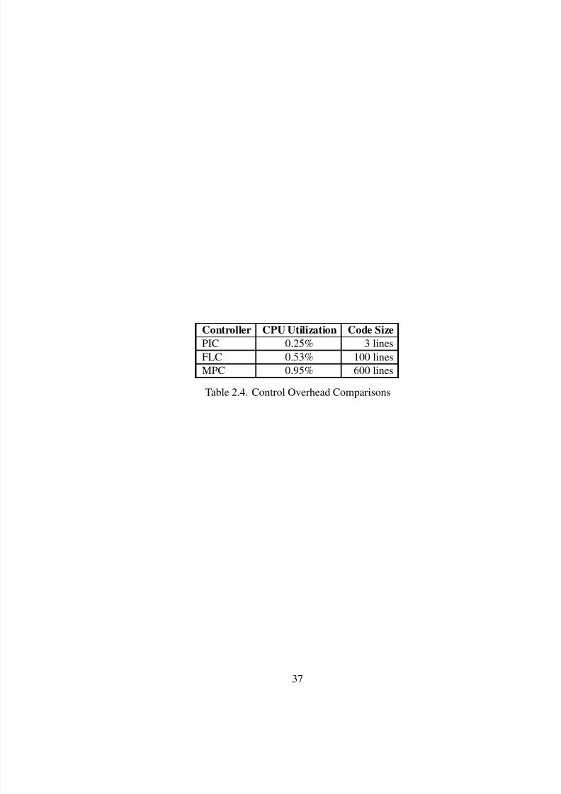
7/31/2019 Mehmet Tez
http://slidepdf.com/reader/full/mehmet-tez 47/95
Controller CPU Utilization Code Size
PIC 0.25% 3 linesFLC 0.53% 100 linesMPC 0.95% 600 lines
Table 2.4. Control Overhead Comparisons
37
7/31/2019 Mehmet Tez
http://slidepdf.com/reader/full/mehmet-tez 48/95
Chapter 3
Bandwidth Consumption Control and Service Differentiation for
Video Streaming
For real-time streaming, a streaming server may take a greedy approach, in which
it simply transmits every frame with the highest possible quality. As a result, however,
multimedia streams may starve other applications, e.g., file transfer, web surfing, email,
and instant messaging in smart homes and buildings. Thus, a system administrator may
specify the bit rate bound for streaming. Also, different videos may have different levels of
importance. For instance, a live stream of the cradle in the baby’s room may have a higher
degree of importance than a movie. Hence, the quality of videos need to be differentiated
according to their importance to ef ficiently utilize limited resources.
To bound the bandwidth usage of streaming, in this chapter, we leverage the layered
encoding technique, in which a video frame consists of a base layer and multiple enhance-
ment layers. We always transmit the base layer, because it is required to display a scene.
However, under overload, we degrade the video quality by dropping high enhancement
layers without affecting the underlying layers, if necessary, to support the specified bit rate
bound. A key challenge is how to determine how many enhancement layers to transmit
for concurrent video streams to support the specified bit rate bound. This is not a triv-
ial problem, since the size of a frame consisting of a base layer and enhancement layers
may significantly vary in time depending on the complexity of the scenes and their inter-
relations in a video. Figure 3.1 is a plot of base-layer size for a single stream and shows the
varying nature of a frame size clearly. Also, new multimedia streaming sessions may start,
38
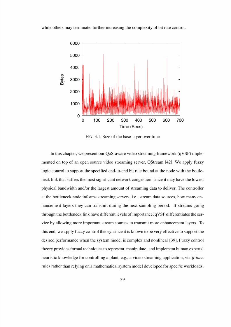
7/31/2019 Mehmet Tez
http://slidepdf.com/reader/full/mehmet-tez 49/95
while others may terminate, further increasing the complexity of bit rate control.
0
1000
2000
3000
4000
5000
6000
0 100 200 300 400 500 600 700
B y t e s
Time (Secs)
FIG. 3.1. Size of the base-layer over time
In this chapter, we present our QoS-aware video streaming framework (qVSF) imple-
mented on top of an open source video streaming server, QStream [42]. We apply fuzzy
logic control to support the specified end-to-end bit rate bound at the node with the bottle-neck link that suffers the most significant network congestion, since it may have the lowest
physical bandwidth and/or the largest amount of streaming data to deliver. The controller
at the bottleneck node informs streaming servers, i.e., stream data sources, how many en-
hancement layers they can transmit during the next sampling period. If streams going
through the bottleneck link have different levels of importance, qVSF differentiates the ser-
vice by allowing more important stream sources to transmit more enhancement layers. To
this end, we apply fuzzy control theory, since it is known to be very effective to support the
desired performance when the system model is complex and nonlinear [39]. Fuzzy control
theory provides formal techniques to represent, manipulate, and implement human experts’
heuristic knowledge for controlling a plant, e.g., a video streaming application, via if-then
rules rather than relying on a mathematical system model developed for specific workloads,
39
7/31/2019 Mehmet Tez
http://slidepdf.com/reader/full/mehmet-tez 50/95
e.g., specific video streams.
qVSF is implemented as a middleware without requiring a change of routers or switches.
For performance evaluation, we have run experiments across the shared department net-
work in the Department of Computer Science at SUNY Binghamton where a considerable
number of different applications usually coexist at the same time. The performance eval-
uation results show that qVSF can support the specified end-to-end bit rate bound. For
ef ficient utilization of the bounded bandwidth, it also differentiates the service by transmit-
ting more enhancement layers for more important streams without severely degrading the
visual quality of low priority video streams.
The rest of the chapter is organized as follows. Section 3.1 describes the architec-
ture of qVSF as well as the rate control and service differentiation schemes. Section 3.2
describes the design of our fuzzy control scheme. Section 3.5 presents the performance
evaluation results. Key related work is reviewed in Section 5.2. Finally, Section 3.6 con-
cludes the chapter and discusses future work.
3.1 System Architecture and Service Differentiation
In this chapter, we adopt the UDP protocol for video streaming. We do not use the TCP
protocol as the AIMD (additive increase and multiplicative decrease) nature of the TCP
congestion control mechanism may adversely affect the timeliness of video streams. Our
approach is reasonable, since a few packet losses could be tolerated for media streaming,
but large delays due to retransmissions and transmission rate reductions caused by the TCP
congestion control protocol may considerably impair the user perceived QoS. We control
the transmission rate of UDP flows for streaming, while differentiating the video quality
between flows.
In our approach, frames are transmitted in an EDF (earliest deadline first) manner.
Thus, the frame with the shortest playtime deadline is transmittedfirst. Figure 3.2 shows the
structure of qVSF that consists of the admission controller (AC), streaming engine, fuzzy
controller, service differentiator (Diff), and chopper. A description of these components
40
7/31/2019 Mehmet Tez
http://slidepdf.com/reader/full/mehmet-tez 51/95
E n gi n e
S t r e a mi n g
C h o p p e r
C on t r ol l e r
r(k)Diff
RS
δ b(k)
QoS Adaptation
Streams UpstreamAC
StreamingRequests
FIG. 3.2. QoS-Aware Streaming Structure
and their interactions follows.
Admission Control. A straightforward approach to admission control may rely on the
peak bit rate requirement of a video stream. However, this simplistic approach is too pes-
simistic. As the frame size may significantly vary over time, a reservation approach based
on the peak bit rate can waste a large fraction of the reserved bandwidth for most of the
time. Also, carefully dropping a subset of enhancement layers under overload might not
severely degrade the user perceived QoS, while considerably reducing the bandwidth con-
sumptions. For these reasons, we take an optimistic approach to admission control that ac-
cepts a streaming request as long as its average bit rate computed at the video encoding time
can be met without affecting the existing streams. Suppose there are m multimedia streams
already in the system and stream j(1 ≤ j ≤ m) requires r j average bps (bits per second).
When a new streaming request arrives, the AC in Figure 3.2 admits it, if r new +∑m j=1 r j ≤ Rs
where r new is the required average bit rate of the newly incoming request and Rs is the bit
rate bound specified by a system administrator.
Fuzzy Control. The stream engine periodically transmits frames. Even if the sum of the
41
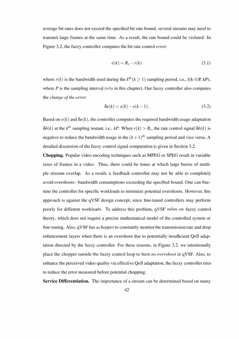
7/31/2019 Mehmet Tez
http://slidepdf.com/reader/full/mehmet-tez 52/95
average bit rates does not exceed the specified bit rate bound, several streams may need to
transmit large frames at the same time. As a result, the rate bound could be violated. In
Figure 3.2, the fuzzy controller computes the bit rate control error :
e(k ) = Rs − r (k ) (3.1)
where r (k ) is the bandwidth used during the k th (k ≥ 1) sampling period, i.e., [(k-1)P, kP),
where P is the sampling interval (=1s in this chapter). Our fuzzy controller also computes
the change of the error :
δe(k ) = e(k ) − e(k − 1). (3.2)
Based on e(k ) and δe(k ), the controller computes the required bandwidth usage adaptation
δb(k ) at the k th sampling instant, i.e., kP. When r (k ) > Rs, the rate control signal δb(k ) is
negative to reduce the bandwidth usage in the (k + 1)th sampling period and vice versa. A
detailed discussion of the fuzzy control signal computation is given in Section 3.2.
Chopping. Popular video encoding techniques such as MPEG or SPEG result in variable
sizes of frames in a video. Thus, there could be times at which large bursts of multi-
ple streams overlap. As a result, a feedback controller may not be able to completely
avoid overshoots−bandwidth consumptions exceeding the specified bound. One can fine-
tune the controller for specific workloads to minimize potential overshoots. However, this
approach is against the qVSF design concept, since fine-tuned controllers may perform
poorly for different workloads. To address this problem, qVSF relies on fuzzy control
theory, which does not require a precise mathematical model of the controlled system or
fine-tuning. Also, qVSF has a chopper to constantly monitor the transmission rate and drop
enhancement layers when there is an overshoot due to potentially insuf ficient QoS adap-tation directed by the fuzzy controller. For these reasons, in Figure 3.2, we intentionally
place the chopper outside the fuzzy control loop to have no overshoot in qVSF. Also, to
enhance the perceived video quality via effective QoS adaptation, the fuzzy controller tries
to reduce the error measured before potential chopping.
Service Differentiation. The importance of a stream can be determined based on many
42
7/31/2019 Mehmet Tez
http://slidepdf.com/reader/full/mehmet-tez 53/95
factors such as the number of individuals interested in the stream or the importance of the
content itself. In this chapter, we assume that weights, i.e., importance levels, of streams
are given by users based on their subjective notion of relative importance among video
streams. Given the bandwidth usage control signal δb(k ), we adapt QoS based on the
relative weights at times of stream bursts to support the bit rate bound, while differentiating
services for ef ficient bandwidth utilization.
In the current version of qVSF, each client specifies an initial weight when it requests
a multimedia stream. For stream j, let wi j and we
j represent the initial weight and effective
weight, respectively. The effective weight is computed: we j = wi
j/∑n j=1 wi
j where n is the
total number of streams. When a new streaming request is accepted, the effective weights
are recomputed. Thus, it always holds that ∑n j=1 we j = 1.
Effective weights are used to distribute the control signal δb(k ) to streams. When the
network is congested, low weight streams are forced to drop more enhancement layers.
When the network is underutilized, higher importance streams can transmit more enhance-
ment layers. Separately, the priority mapper of QStream [42] assigns a priority to each
layer ranging from 0 to 15 where 15 is the highest priority. These priorities are assigned
according to the utility of a layer estimated in terms of the user perceived QoS considering
the type of the frame (i.e., I, B, or P) and its rank in the layer hierarchy. To support band-
width control and service differentiation at the same time, qVSF performs the following
procedure at the k th (≥ 1) sampling instant.
1. Compute the bandwidth control signal δb(k ).
2. Let N p represent the number of priority levels. In QStream, N p = 16. Compute the
transmission threshold for s j, i.e., stream j: θ j(k ) = θ j(k −1)−δb(k ) · f (δb(k ), we j) ·
( N p − 1) where
• f (δb(k ), we j) = we
j if δb(k ) ≥ 0.
• f (δb(k ), we j) = 1 − we
j otherwise.
If θ j > N p − 1, set θ j = N p − 1. If θ j < 0, set θ j = 0. Note that ∀ j θ j(0) = N p − 1.
43
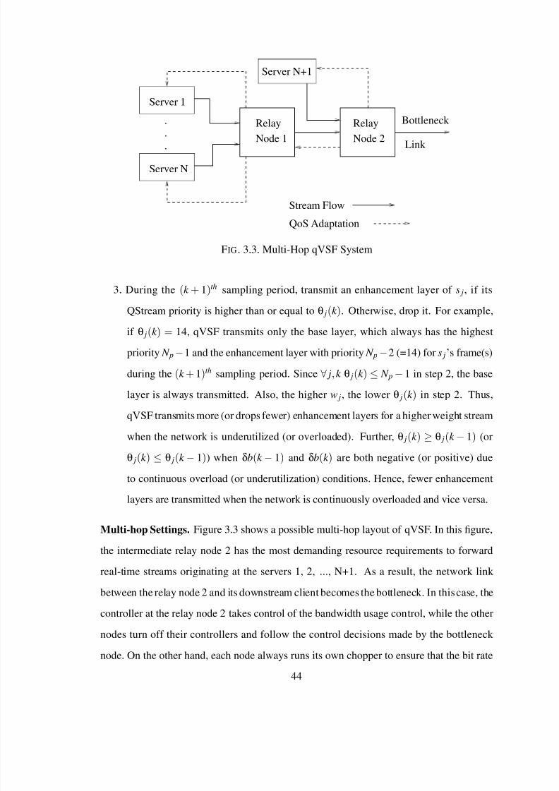
7/31/2019 Mehmet Tez
http://slidepdf.com/reader/full/mehmet-tez 54/95
Relay
Node 1
Relay
Node 2 Link
Bottleneck
Server N+1
Server N
Server 1
.
..
Stream Flow
QoS Adaptation
FIG. 3.3. Multi-Hop qVSF System
3. During the (k + 1)th sampling period, transmit an enhancement layer of s j, if its
QStream priority is higher than or equal to θ j(k ). Otherwise, drop it. For example,
if θ j(k ) = 14, qVSF transmits only the base layer, which always has the highest
priority N p −1 and the enhancement layer with priority N p −2 (=14) for s j’s frame(s)
during the (k + 1)th sampling period. Since ∀ j, k θ j(k ) ≤ N p − 1 in step 2, the base
layer is always transmitted. Also, the higher w j, the lower θ j(k ) in step 2. Thus,
qVSF transmits more (or drops fewer) enhancement layers for a higher weight stream
when the network is underutilized (or overloaded). Further, θ j(k ) ≥ θ j(k − 1) (or
θ j(k ) ≤ θ j(k − 1)) when δb(k − 1) and δb(k ) are both negative (or positive) due
to continuous overload (or underutilization) conditions. Hence, fewer enhancement
layers are transmitted when the network is continuously overloaded and vice versa.
Multi-hop Settings. Figure 3.3 shows a possible multi-hop layout of qVSF. In this figure,
the intermediate relay node 2 has the most demanding resource requirements to forwardreal-time streams originating at the servers 1, 2, ..., N+1. As a result, the network link
between the relay node 2 and its downstream client becomes the bottleneck. In thiscase, the
controller at the relay node 2 takes control of the bandwidth usage control, while the other
nodes turn off their controllers and follow the control decisions made by the bottleneck
node. On the other hand, each node always runs its own chopper to ensure that the bit rate
44

7/31/2019 Mehmet Tez
http://slidepdf.com/reader/full/mehmet-tez 55/95
on its outgoing link does not exceed Rs. Thus, the end-to-end bandwidth usage does not
exceed Rs. In summary, via fuzzy control and chopping, we ensure that the UDP traf fic
rate for streaming conforms to the bit rate bound specified by the system administrator.
By supporting rate control and service differentiation, our work could provide a basis for
important real-time and non-real-time applications such as network services in smart homes
and buildings. A system administrator can allocate the bandwidth with the confidence that
the allocated bandwidth limits and service differentiation policy will be enforced by our
approach. A thorough investigation of bandwidth allocation between different types of
applications, e.g., video streaming and file transfer, in smart environments is reserved for
future work.
3.2 Fuzzy Control of the Transmission Rate
In this section, the design of our fuzzy logic controller is discussed. For the clarify of
presentation, we convert the rate control problem to the problem of controlling the utiliza-
tion of the bottleneck link. To achieve the target utilization, our fuzzy controller computes
the workload control signal based on the error e(k ) and change of the error δe(k ) redefined
as follows:
e(k ) = U s − u(k ) = U s − r (k )/ Rs (3.3)
δe(k ) = e(k ) − e(k − 1) (3.4)
where the utilization u(k ) is the total bandwidth utilization in the k th sampling period. In
this chapter, we set the target utilization U s = 1 to fully utilize Rs. As discussed before,
there is no overshoot due to possible chopping.
Based on e(k ) and δe(k ) computed in Eq. 3.3 and Eq. 3.4, the fuzzy rate controller
computes the required utilization adjustment δu(k ) for the next sampling period. K e, K δe,
and K Δr in Figure 3.4 are control gains tuned by trial and error. Specifically, we choose
K e = 1.0, K δe = 0.5, and K Δr = 0.1. Intuitively, e(k ) at the k th sampling instant needs
to be fully considered, while δe(k ) and (especially) δu(k ) need to be damped to avoid
45
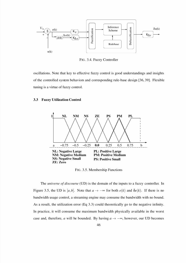
7/31/2019 Mehmet Tez
http://slidepdf.com/reader/full/mehmet-tez 56/95
d/dte(k)
SchemeInference
Rulebase F u z z i f i c a t i o n
D e f u z z i f i c a t i o n
K e
eK
−
ΔΔ
+Σ
s e(k)
Δ r
u(k)
U
K
u(k)δ
FIG. 3.4. Fuzzy Controller
oscillations. Note that key to effective fuzzy control is good understandings and insights
of the controlled system behaviors and corresponding rule-base design [36, 39]. Flexible
tuning is a virtue of fuzzy control.
3.3 Fuzzy Utilization Control
NL: Negative Large
NS: Negative SmallNM: Negative Medium
ZE: Zero
PL: Positive LargePM: Positive Medium
NL NM NS ZE PS PM PL1
ba 0.25 0.5 0.75
PS: Positive Small
0.0−0.25−0.5−0.75
FIG. 3.5. Membership Functions
The universe of discourse (UD) is the domain of the inputs to a fuzzy controller. InFigure 3.5, the UD is [a, b]. Note that a → −∞ for both e(k ) and δe(k ). If there is no
bandwidth usage control, a streaming engine may consume the bandwidth with no bound.
As a result, the utilization error (Eq 3.3) could theoretically go to the negative infinity.
In practice, it will consume the maximum bandwidth physically available in the worst
case and, therefore, a will be bounded. By having a → −∞, however, our UD becomes
46
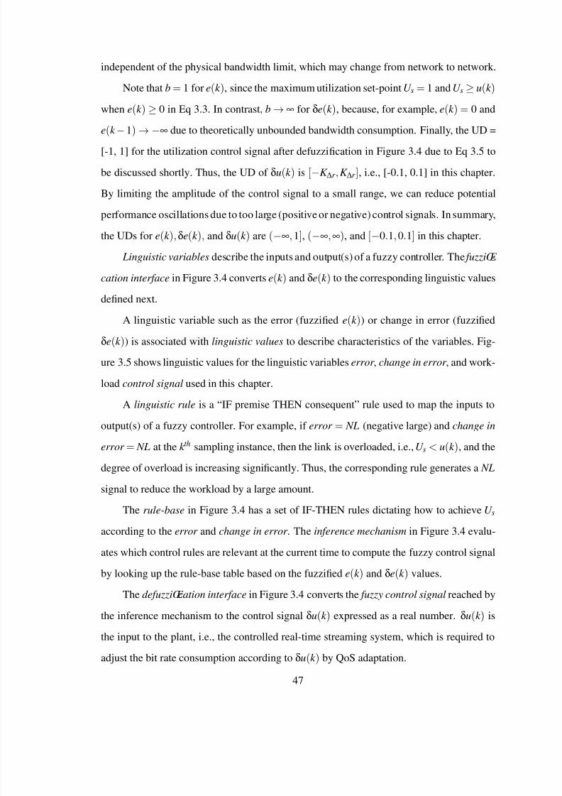
7/31/2019 Mehmet Tez
http://slidepdf.com/reader/full/mehmet-tez 57/95
independent of the physical bandwidth limit, which may change from network to network.
Note that b = 1 for e(k ), since the maximum utilization set-point U s = 1 and U s ≥ u(k )
when e(k ) ≥ 0 in Eq 3.3. In contrast, b → ∞ for δe(k ), because, for example, e(k ) = 0 and
e(k − 1) → −∞ due to theoretically unbounded bandwidth consumption. Finally, the UD =
[-1, 1] for the utilization control signal after defuzzification in Figure 3.4 due to Eq 3.5 to
be discussed shortly. Thus, the UD of δu(k ) is [−K Δr , K Δr ], i.e., [-0.1, 0.1] in this chapter.
By limiting the amplitude of the control signal to a small range, we can reduce potential
performance oscillations due to too large (positive or negative) control signals. In summary,
the UDs for e(k ),δe(k ), and δu(k ) are (−∞, 1], (−∞,∞), and [−0.1, 0.1] in this chapter.
Linguistic variables describe the inputs and output(s) of a fuzzy controller. The fuzzifi -
cation interface in Figure 3.4 converts e(k ) and δe(k ) to the corresponding linguistic values
defined next.
A linguistic variable such as the error (fuzzified e(k )) or change in error (fuzzified
δe(k )) is associated with linguistic values to describe characteristics of the variables. Fig-
ure 3.5 shows linguistic values for the linguistic variables error , change in error , and work-
load control signal used in this chapter.
A linguistic rule is a “IF premise THEN consequent” rule used to map the inputs to
output(s) of a fuzzy controller. For example, if error = NL (negative large) and change in
error = NL at the k th sampling instance, then the link is overloaded, i.e., U s < u(k ), and the
degree of overload is increasing significantly. Thus, the corresponding rule generates a NL
signal to reduce the workload by a large amount.
The rule-base in Figure 3.4 has a set of IF-THEN rules dictating how to achieve U s
according to the error and change in error . The inference mechanism in Figure 3.4 evalu-
ates which control rules are relevant at the current time to compute the fuzzy control signalby looking up the rule-base table based on the fuzzified e(k ) and δe(k ) values.
The defuzzifi cation interface in Figure 3.4 converts the fuzzy control signal reached by
the inference mechanism to the control signal δu(k ) expressed as a real number. δu(k ) is
the input to the plant, i.e., the controlled real-time streaming system, which is required to
adjust the bit rate consumption according to δu(k ) by QoS adaptation.
47
7/31/2019 Mehmet Tez
http://slidepdf.com/reader/full/mehmet-tez 58/95
The horizontal axis of Figure 3.5 represents e(k ) or δe(k ) and the vertical axis indicates
the membership value. A membership function (MF) quantifies the certainty an e(k ) (or
δe(k )) value to be associated with a certain linguistic value. For MFs, we use symmetric
triangles of an equal base and 50% overlap with adjacent MFs. A triangular MF is one
of the most popular MF’s in fuzzy control [39]. For example, suppose e(k ) = 0.25. In
Figure 3.5, μPS (0.25) = 1; that is, 0.25 belongs to the fuzzy set PS with certainty 1.
Based on the fuzzified e(k ) and δe(k ), the inference mechanism in Figure 3.4 deter-
mines which rules to apply at the k th sampling instance. For example, suppose e(k ) = 0.25
and δe(k ) = 0.0625. According to Figure 3.5, the certainty μPS (0.25) = 1 for e(k ) and
μ ZE (0.0625) = 0.75 and μPS (0.0625) = 0.25 for δe(k ). To compute the certainty value of
the premise in the corresponding IF premise THEN consequent rule(s), we take the mini-
mum between the certainty values of e(k ) and δe(k ), following the one of the most common
approaches [36,39, 54]. Thus,μ(error , change in error ) =μ(PS , ZE ) = min{1, 0.75} = 0.75
and μ(PS , PS ) = min{1,0.25} = 0.25.
By referring to our rule base in Table 3.1, the inference engine finds that rule(PS , ZE )
= PS and rule(PS , PS ) = PM . Let μ(i, j) denote the membership function and c(i, j) denote
the center of the MF of the consequent of the rule(i, j). For triangle MFs, the center is the
value on the x axis at the middle of the triangle [39]. For example, in Figure 3.5, the center
of PS and PM is 0.25 and 0.5, respectively. Then the fuzzy utilization control output is:
δu(k ) =∑i, j c(i, j) ·μ(i, j)
∑i, jμ(i, j)(3.5)
In the previous example, the defuzzified control signal δu(k ) = 0.25·0.75+0.5·0.250.75+0.25 = 0.3125.
For more information about fuzzy control, readers are referred to [39]. A discussion of key
ideas behind our rule base design follows.
3.4 Fuzzy Rule Base
As shown in Figure 3.6, there are five zones that characterize the utilization con-
troller’s action, from which we derive the rule-base for fuzzy utilization control described
48

7/31/2019 Mehmet Tez
http://slidepdf.com/reader/full/mehmet-tez 59/95
1
2
4 U t i l i z a t i o n
Time
Overshoot
3
Undershoot
Set−point
5
FIG. 3.6. Utilization Control Characteristics
in Table 3.1:
1. If e(k ) is positive and δe(k ) is negative, the actual utilization is smaller than the target
utilization, but it comes closer to the set-point. The controller applies a small signal
to avoid a potential overshoot while increasing the utilization.
2. If e(k ) is negative and δe(k ) is negative, the actual utilization is larger than the set-
point and it is further increasing. The controller must reduce the load to reverse the
current trend.
3. e(k ) is negative and δe(k ) is positive, the actual utilization is higher than the target
utilization, but it comes closer to the set-point. Since the actual utilization is converg-
ing to the target, the controller applies a small signal to avoid a potential undershoot,
i.e., underutilization, while reducing the utilization.
4. e(k ) is positive and δe(k ) is positive, the actual utilization is lower than the set-point
and it is further decreasing. Thus, the controller increases the utilization to reverse
the current trend.
5. If |e(k )| < ε and |δe(k )| < ε where ε is a predefined small positive real number, the
utilization converges to the set-point and |e(k )| and |δe(k )| are small. Hence, the
utilization adjustment δu(k ) = 0.
49

7/31/2019 Mehmet Tez
http://slidepdf.com/reader/full/mehmet-tez 60/95
e/ δe NL NM NS ZE PS PM PL
NL NL NL NL NL NM NS ZE
NM NL NL NL NM NS ZE PS
NS NL NL NM NS ZE PS PM
ZE NL NM NS ZE PS PM PL
PS NM NS ZE PS PM PL PLPM NS ZE PS PM PL PL PL
PL ZE PS PM PL PL PL PL
Table 3.1. Utilization Control Rules
Overall, our fuzzy logic control is lightweight, only requiring a small rule-base, ef fi-
cient table look-ups, and control signal computation (Eq 3.3 − Eq 3.5).
3.5 Performance Evaluation
The results given in this section are taken from a streaming session during which four
clients are served. The duration of the session was 13 minutes. Client requests were sent
at arbitrary times within the first minute of the session. Each client requested a different
video from the server over our department network. The set-point for transmission rate is
set as 2 Mbps, while the four streamed videos require approximately 1.8 Mbps in average.The choice of the set-point was an arbitrary one in our case, driven by our desire to create
a harsh environment. For the same settings, QStream [42] without our QoS management
schemes often consumes more than 4Mbps. We have considered different settings too.
However, due to space limitations, we only present key performance evaluation results.
Figure 3.7 shows the bandwidth usage of the streaming server for the entire session.
Transient bandwidth is the transmission rate of the server measured every second. The av-
erage bandwidth usage at time t is the average bandwidth consumption over the time period
[0, t]. As shown in the figure, cooperation between the controller and chopper eliminates
overshoots for the entire streaming session period. Without chopping, our fuzzy controller
experiences approximately 10 overshoots in the 13 minute experiment and the largest tran-
sient bandwidth usage was approximately 2.5Mbps. Moreover, due to the nature of video
50
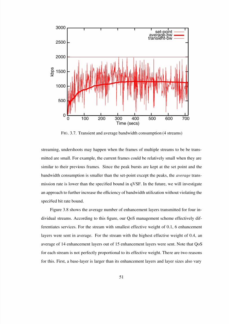
7/31/2019 Mehmet Tez
http://slidepdf.com/reader/full/mehmet-tez 61/95
0
500
1000
1500
2000
2500
3000
0 100 200 300 400 500 600 700
k b p s
Time (secs)
set-pointaverage-bwtransient-bw
FIG. 3.7. Transient and average bandwidth consumption (4 streams)
streaming, undershoots may happen when the frames of multiple streams to be be trans-
mitted are small. For example, the current frames could be relatively small when they are
similar to their previous frames. Since the peak bursts are kept at the set point and the
bandwidth consumption is smaller than the set-point except the peaks, the average trans-
mission rate is lower than the specified bound in qVSF. In the future, we will investigate
an approach to further increase the ef ficiency of bandwidth utilization without violating the
specified bit rate bound.
Figure 3.8 shows the average number of enhancement layers transmitted for four in-
dividual streams. According to this figure, our QoS management scheme effectively dif-
ferentiates services. For the stream with smallest effective weight of 0.1, 6 enhancement
layers were sent in average. For the stream with the highest effective weight of 0.4, an
average of 14 enhancement layers out of 15 enhancement layers were sent. Note that QoS
for each stream is not perfectly proportional to its effective weight. There are two reasons
for this. First, a base-layer is larger than its enhancement layers and layer sizes also vary
51
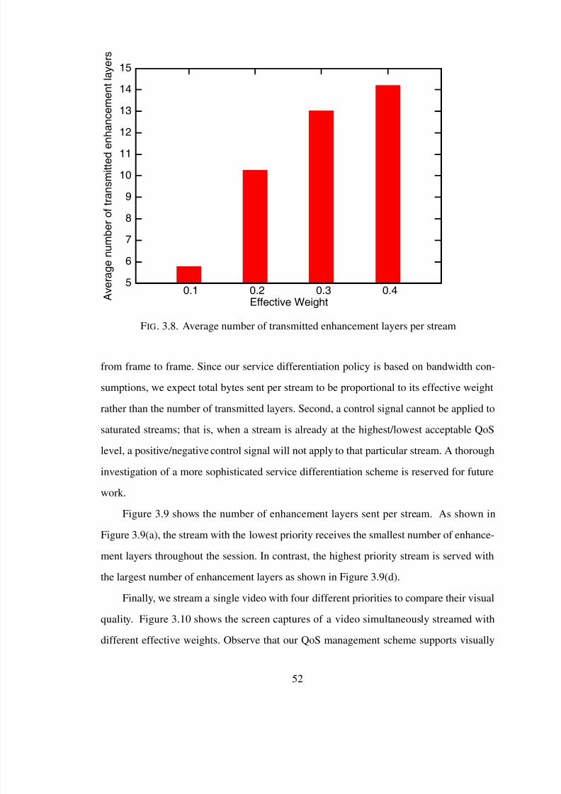
7/31/2019 Mehmet Tez
http://slidepdf.com/reader/full/mehmet-tez 62/95
5
6
7
8
9
10
11
12
13
14
15
0.40.30.20.1 A v e r a
g e n u m b e r o f t r a n s m i t t e d e n h a n c e m e n t l a y e r s
Effective Weight
FIG. 3.8. Average number of transmitted enhancement layers per stream
from frame to frame. Since our service differentiation policy is based on bandwidth con-
sumptions, we expect total bytes sent per stream to be proportional to its effective weight
rather than the number of transmitted layers. Second, a control signal cannot be applied to
saturated streams; that is, when a stream is already at the highest/lowest acceptable QoS
level, a positive/negative control signal will not apply to that particular stream. A thorough
investigation of a more sophisticated service differentiation scheme is reserved for future
work.
Figure 3.9 shows the number of enhancement layers sent per stream. As shown in
Figure 3.9(a), the stream with the lowest priority receives the smallest number of enhance-
ment layers throughout the session. In contrast, the highest priority stream is served with
the largest number of enhancement layers as shown in Figure 3.9(d).
Finally, we stream a single video with four different priorities to compare their visual
quality. Figure 3.10 shows the screen captures of a video simultaneously streamed with
different effective weights. Observe that our QoS management scheme supports visually
52
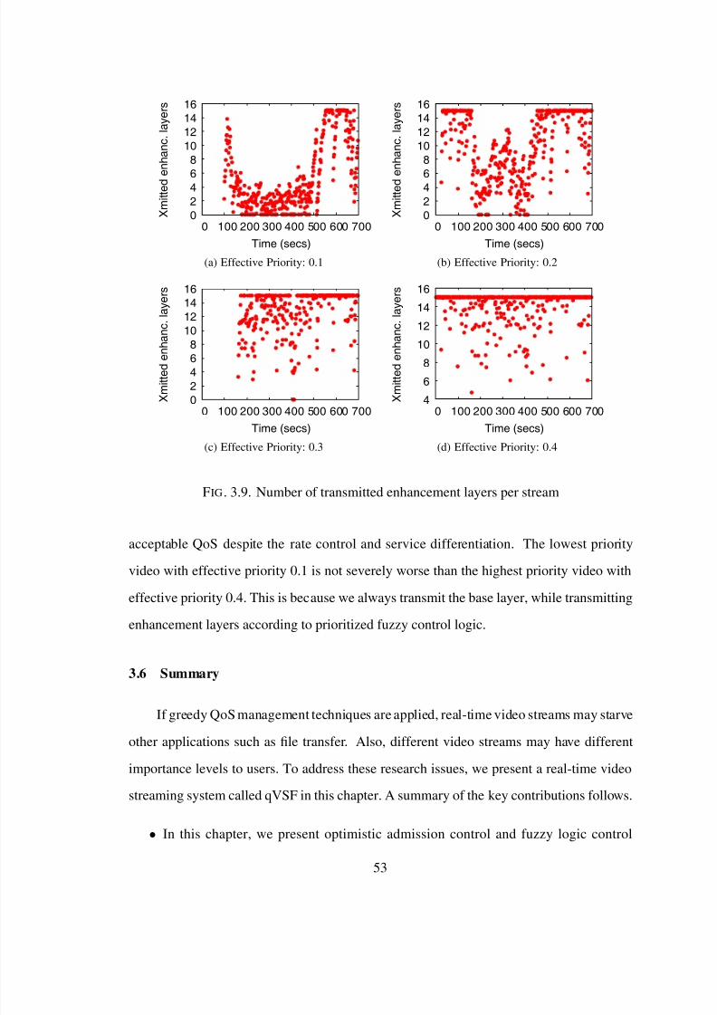
7/31/2019 Mehmet Tez
http://slidepdf.com/reader/full/mehmet-tez 63/95
0
2
46
8
10
12
14
16
0 100 200 300 400 500 600 700 X m i t t e d e n h a n c . l a y e r s
Time (secs)
(a) Effective Priority: 0.1
0
2
46
8
10
12
14
16
0 100 200 300 400 500 600 700 X m i t t e d e n h a n c . l a y e r s
Time (secs)
(b) Effective Priority: 0.2
0
2
46
8
10
12
14
16
0 100 200 300 400 500 600 700 X m i t t e d e n h a n c . l a y e r s
Time (secs)
(c) Effective Priority: 0.3
4
6
8
10
12
14
16
0 100 200 300 400 500 600 700 X m i t t e d e n h a n c . l a y e r s
Time (secs)
(d) Effective Priority: 0.4
FIG. 3.9. Number of transmitted enhancement layers per stream
acceptable QoS despite the rate control and service differentiation. The lowest priority
video with effective priority 0.1 is not severely worse than the highest priority video with
effective priority 0.4. This is because we always transmit the base layer, while transmitting
enhancement layers according to prioritized fuzzy control logic.
3.6 Summary
If greedy QoS management techniques are applied, real-time video streams may starve
other applications such as file transfer. Also, different video streams may have different
importance levels to users. To address these research issues, we present a real-time video
streaming system called qVSF in this chapter. A summary of the key contributions follows.
• In this chapter, we present optimistic admission control and fuzzy logic control
53
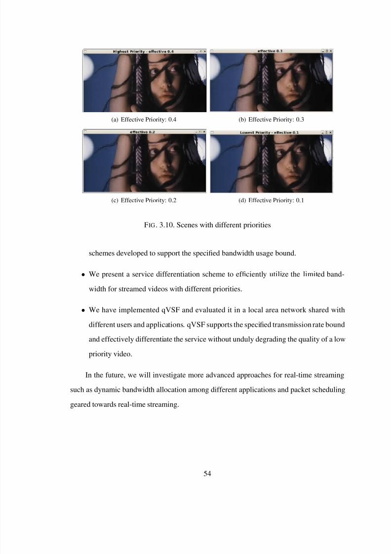
7/31/2019 Mehmet Tez
http://slidepdf.com/reader/full/mehmet-tez 64/95
(a) Effective Priority: 0.4 (b) Effective Priority: 0.3
(c) Effective Priority: 0.2 (d) Effective Priority: 0.1
FIG. 3.10. Scenes with different priorities
schemes developed to support the specified bandwidth usage bound.
• We present a service differentiation scheme to ef ficiently utilize the limited band-
width for streamed videos with different priorities.
• We have implemented qVSF and evaluated it in a local area network shared with
different users and applications. qVSF supports the specified transmission rate bound
and effectively differentiate the service without unduly degrading the quality of a low
priority video.
In the future, we will investigate more advanced approaches for real-time streaming
such as dynamic bandwidth allocation among different applications and packet scheduling
geared towards real-time streaming.
54
7/31/2019 Mehmet Tez
http://slidepdf.com/reader/full/mehmet-tez 65/95
Chapter 4
Active Queue Management via Event-Driven Feedback Control
Congestion control and avoidance is critical. Packets can be dropped before reaching
their destinations due to congestion, wasting all the resources consumed by them. It is
known that, in an extreme case, congestion collapse may happen causing users suffer se-
vere network performance degradation [20]. For congestion control and avoidance, AQM
(Active Queue Management) has been investigated. Usually, AQM is implemented in gate-
ways that can distinguish between the propagation delay and persistent queuing delay for
effective congestion detection. As a gateway is shared by many active connections with a
wide range of round trip times, delay tolerances, and throughput requirements, decisions
about the duration and magnitude of transient congestion to be allowed at the gateway are
best made by the gateway itself.
The notion of feedback control has been applied to manage the queue length. RED
(Random Early Detection) [13], which is one of the earliest approaches for AQM, controls
the queue length based on ad hoc feedback control. The objective of RED is to detect any
incipient congestion early and provide congestion notification to the sources to let them re-
duce their transmission rates before packets are dropped due to overflow in network queues.
To detect congestion, RED keeps track of an exponentially weighted moving average of the
queue length. If the average queue length exceeds a minimum threshold, RED randomly
drops or marks packets with an explicit congestion notification bit. Additionally, all pack-
ets are marked or dropped if the average queue length exceeds the specified maximum
threshold. RED is an ad hoc feedback-based approach, as it neither mathematically mod-
els the TCP and queue length dynamics nor develops a feedback controller for congestion
55

7/31/2019 Mehmet Tez
http://slidepdf.com/reader/full/mehmet-tez 66/95
7/31/2019 Mehmet Tez
http://slidepdf.com/reader/full/mehmet-tez 67/95
this reason, RED is designed to be event-driven. Our approach is also event-driven.
Further, it is based on a rigorous mathematical model and formal control theory
[15,40] unlike RED. Thus, we can apply well established control theory [15,40]
to tune and mathematically analyze and support the stability of our feedback-based
congestion control scheme.
• If a large number of packets arrive in a short time interval, event-driven controller
autonomously executes more often. As a result, the latency for congestion control
reduces, enhancing the reactiveness to bursty network loads. In contrast, a time-
driven controller has to wait until the next sampling period even in the presence of a
dramatic increase in packet arrivals during the current sampling period.
• If the packet arrival rate decreases, an event-driven controller automatically adapts
itself to execute less frequently. As a result, under light loads, it consumes less
computational resources than a time-driven controller does.
To support event-driven congestion control, we convert the time domain TCP and
queue model [18, 35] to the corresponding spatial domain−event domain−model. A sum-
mary of our key contributions follows:
• We transform the time-domain nonlinear TCP and queue model [18] to the corre-
sponding spatial-domain model. For this transformation and event-driven controller
design, we adapt the event-driven control theoretic techniques [15] developed for
motor synchronization. The key idea behind [15] is to measure the time between an-
gular movements around a motor’s axis to compute the speed and acceleration in an
event-driven fashion rather than calculating the speed and acceleration using a fixed
(periodic) sampling rate. In this chapter, we adapt this approach to measure the time
taken for a specified number of packets to arrive at the queue. Thus, our approach is
not tied to a fixed sampling rate but purely driven by events, i.e., packet arrivals.
• We linearize the spatial-domain nonlinear model and design an event-driven con-
troller based on the linearized model. The basic approach is similar to [19] that
57

7/31/2019 Mehmet Tez
http://slidepdf.com/reader/full/mehmet-tez 68/95
linearize the time-driven model; however, we linearize the event-driven model in the
spatial domain unlike [19].
• Also, we thoroughly evaluate the performance of our approach via an extensive
simulation study in OMNeT++ [37]. We compare it to five advanced approaches
for AQM: (1) RED [13] with the ’gentle’ parameter turned on, (2) the time-driven
feedback-based Proportional Integral (PI) congestion controller developed by Hollot
et al.[19], (3) Proportional Integral based series compensation, and Position feedback
compensation (PIP) Controller [17], (4) Adaptive Optimized Proportional Controller
(AOPC) [49] and (5) Fuzzy Logic Controller (FLC) [10]. The simulation results
show that our event-driven controller effectively maintains the queue length around
the specified reference, while reducing queue length fluctuations compared to the
tested baseline approaches. At the same time, it achieves shorter E2E (end-to-end)
delays and noticeably smaller E2E delay fluctuations than RED, PI and PIP con-
trollers, while achieving almost the same E2E delays and E2E delay fluctuations
with AOPC and FLC controllers. Further, it is invoked only 8 times per second in
average. In contrast, RED is activated 30 times/s in average while PI [19], PIP [17],
AOPC [49] and FLC [10] congestion controllers are activated 160 times/s.
The remainder of this chapter is organized as follows. A problem formulation is given
in Section 4.1. Our event-driven approach for active queue management is described in Sec-
tion 4.2. The performance of our approach and five baselines is compared in Section 4.8.
Related work is discussed in Section 5.3. Finally, Section 4.9 concludes the chapter and
discusses future work.
4.1 Problem Formulation
This section describes the scope of this chapter, while reviewing the main objectives
of AQM.
AQM aims to support congestion avoidance by controlling the queue length to be
shorter than the specified upper bound, even if the transport layer protocols in the traf fic
58
7/31/2019 Mehmet Tez
http://slidepdf.com/reader/full/mehmet-tez 69/95
sources do not support any congestion control. In this way, AQM aims to reduce the num-
ber of packet drops when a network traf fic burst arrives. Although there is an upper bound
on the queue length, AQM is desired to allow queue length fluctuations to let the queue ab-
sorb bursty traf fic spikes and accommodate transient congestion. This can be accomplished
by either controlling the average queue length instead of the transient queue length or by
employing a low pass filter, such as the integrator in a PID (proportional, integral, and dif-
ferential) or PI controller [40], on the control path. Thus, the queue length limit reflects the
size of bursts needed to be absorbed rather than the steady state queue length desired to be
maintained. Queue length control affects the overall throughput and E2E delay. Especially,
there is a trade-off between throughput and E2E delay. Enforcing a smaller upper bound
on the queue length translates into lower E2E delay, but this comes at the expense of lower
throughput and vice versa.
In AQM, the gateway needs to randomly select a victim connection to drop packets
from. If the gateway drops packets from all connections at the same time, this will result
in global synchronization where all the flows throttle back their transmission rates under
congestion and potentially increase the rates later in a synchronized manner. As a result,
the network performance may oscillate widely. Via random selection, AQM also aims to
avoid biases against bursty traf fi c that is observed, for example, in a Drop Tail queue [13].
Moreover, AQM should be compatible with TCP. Generally, AQM notifies the traf fic
source of a congestion condition implicitly (by dropping packets) or explicitly (by forward-
ing an explicit control notification to sources). Therefore, AQM is appropriate to be used
with TCP flows that can react to congestion detection.
In addition, there are several features desired to be supported by AQM:
• An AQM algorithm is desired to react quickly to workload changes. Ideally, an
overshoot, i.e., the queue length longer than the desired reference value, and settling
time, i.e., the time taken to cancel an overshoot (if any), should be minimal in the
presence of dynamic load changes.
• Even if the load changes abruptly, the algorithm is desired to control the queue length
59
7/31/2019 Mehmet Tez
http://slidepdf.com/reader/full/mehmet-tez 70/95
to be stable and avoid large queue length oscillations.
• The implementation and tuning of the algorithm is desired to be easy.
• It is desirable for the algorithm to not need any further tuning upon load changes.
• The algorithm itself should not consume excessive amounts of system resources.
The bursty nature of network traf fic and dynamic behavior of network components
make these performance criteria dif ficult to meet. RED controls the packet drop rate by
monitoring the average queue length. However, RED lacks a mathematical or control theo-
retic model. Thus, it shows weak performance in the presence of highly dynamic network
traf fi
c [18]. Also, RED has many parameters to tune, which makes it dif fi
cult to obtainbest performance. The time driven controllers such as ([19], [17], [49], [10]) showed su-
perior performance to RED; however, they cannot adapt their sampling rate according to
the network traf fic. Thus, they must be designed in a pessimistic way to support acceptable
performance under heavy loads. As a result, they have to sample the queue length and run
the AQM algorithm unnecessarily often under light loads as discussed before.
To address these problems, we develop an EDC (Event Driven Controller). Different
from most of existing approaches for AQM that is based on either ad hoc event-driven feed-
back control [11–13,38, 44] or time-driven control theoretic techniques [10, 17, 19, 49, 56],
our approach for congestion control leverages both the event-driven nature of the RED
scheme and control theoretic aspect of the feedback PI controller scheme. EDC has only
two parameters to tune for application dependent performance requirements: (1) the de-
sired queue length set-point and (2) event threshold that specifies the number of packet
arrivals that triggers an event. By applying control theoretic techniques [15, 40], we aim
to tune EDC to support its stability. Also, EDC aims to reduce the consumption of system
resources for AQM via systematic event-driven control of the queue length.
60
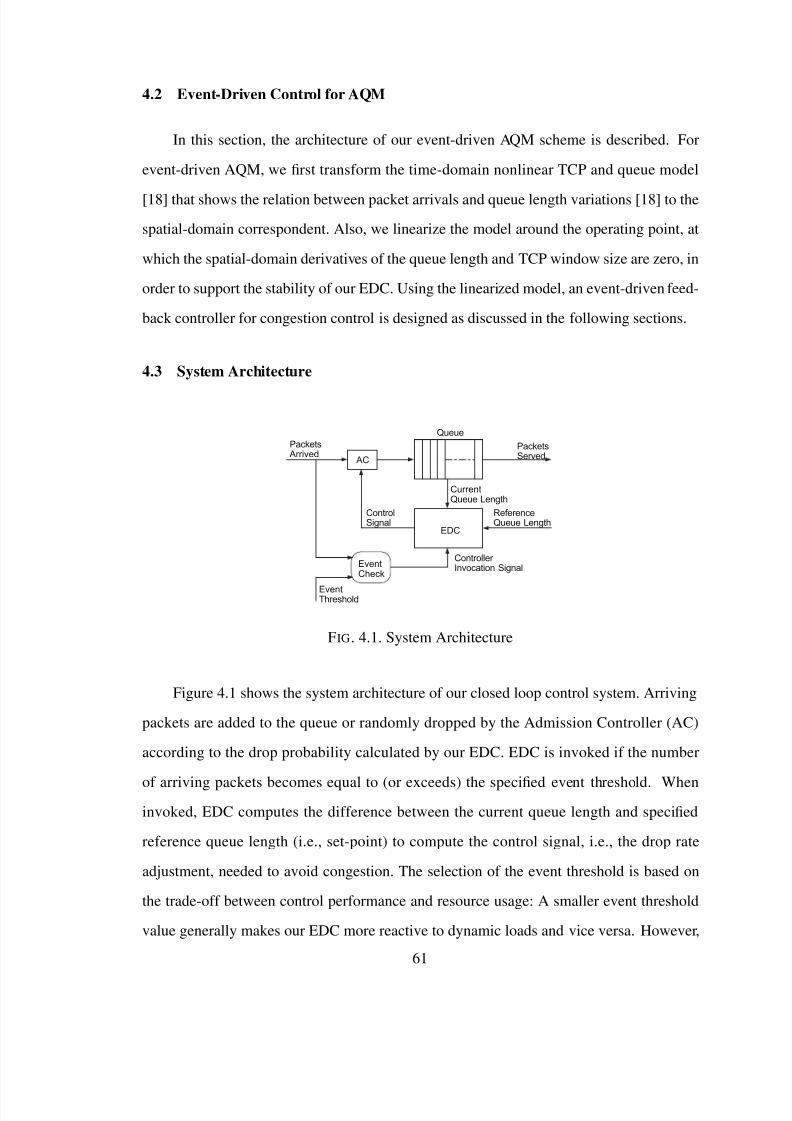
7/31/2019 Mehmet Tez
http://slidepdf.com/reader/full/mehmet-tez 71/95
4.2 Event-Driven Control for AQM
In this section, the architecture of our event-driven AQM scheme is described. For
event-driven AQM, we first transform the time-domain nonlinear TCP and queue model
[18] that shows the relation between packet arrivals and queue length variations [18] to the
spatial-domain correspondent. Also, we linearize the model around the operating point, at
which the spatial-domain derivatives of the queue length and TCP window size are zero, in
order to support the stability of our EDC. Using the linearized model, an event-driven feed-
back controller for congestion control is designed as discussed in the following sections.
4.3 System Architecture
Packets Arrived
PacketsServed
EDC
Queue
AC
EventThreshold
ReferenceQueue Length
CurrentQueue Length
ControlSignal
Controller Invocation SignalEvent
Check
FIG. 4.1. System Architecture
Figure 4.1 shows the system architecture of our closed loop control system. Arriving
packets are added to the queue or randomly dropped by the Admission Controller (AC)
according to the drop probability calculated by our EDC. EDC is invoked if the number
of arriving packets becomes equal to (or exceeds) the specified event threshold. Wheninvoked, EDC computes the difference between the current queue length and specified
reference queue length (i.e., set-point) to compute the control signal, i.e., the drop rate
adjustment, needed to avoid congestion. The selection of the event threshold is based on
the trade-off between control performance and resource usage: A smaller event threshold
value generally makes our EDC more reactive to dynamic loads and vice versa. However,
61

7/31/2019 Mehmet Tez
http://slidepdf.com/reader/full/mehmet-tez 72/95
simply picking the smallest possible event threshold may not be a solution, because too
frequent EDC invocations may consume excessive computational resources at the router.
In our approach, the event threshold is computed based on the network parameters usually
available, such as the link capacity and typical packet size. For example, let us assume
that the link capacity is 10Mbps and the measured average packet size is 1,000 bits. In
this case, to invoke EDC for a number of new packet arrivals estimated to consume 1%
link utilization, the event threshold is set to 100 packets. If many packets arrive in a short
time interval, EDC is invoked frequently and vice versa. From this example, we observe
that, to select the event threshold, we do not need to assume heavy network loads that may
happen only occasionally. Hence, selecting the event threshold is much less complex and
less pessimistic than choosing the sampling period for a time driven controller.
4.4 TCP and Queue Mathematical Models
Let ˙ x denote the time derivative of x. At time t, the following nonlinear differential
equations model the TCP and queue dynamics [18] in the time domain:
W (t ) =1
R(t )
−W (t ) ·W (t − R(t ))
2 R(t − R(t ))
· p(t − R(t ))
q(t ) =W (t )
R(t )· N (t ) −C (4.1)
where W is the expected TCP window size, q is the expected queue length, C is the link
capacity (packets/s), N is the load factor expressed in terms of the number of TCP sessions,
T p is the propagation delay, R is the average round trip time = qC
+ T p (seconds) and p(∈
[0, 1]) is the packet mark/drop probability.
In Eq. 4.1, the queue length q and the window size W are bounded positive quantities;
therefore, q ∈ [0, q] and W ∈ [0,W ] where q and W denote the maximum queue size and
maximum window size, respectively.
62

7/31/2019 Mehmet Tez
http://slidepdf.com/reader/full/mehmet-tez 73/95
4.5 Transformation from Time Domain to Spatial Domain
For event-driven AQM, we transform the window size and queue length models in
Eq. 4.1 to the spatial domain correspondents by applying the techniques presented in [15].
If θ(t ) denotes the number of packets arrived at the queue at time t, the packet arrival
rate at time t is:d θ
dt =
N (t )
R(t )· W (t ) (4.2)
The transformation from the time domain (t ) to the spatial domain (θ) can be performed
based on this relationship. The key idea is to consider θ no longer as a function of time t,
but to let time t be a function of packet arrivals θ. The notation t (θ) then denotes the time at
which θ packets arrived at the queue. With this interpretation,W (θ), R(θ) and N (θ) denote
the window size, round trip time and number of TCP sessions at the time when θ packets
arrive at the queue. Based on this observation, we transform Eq. 4.2 to the event-driven,
spatial-domain as follows:
dt =R(θ)
N (θ) · W (θ)· d θ (4.3)
Let W (θ) =dW
d θ and q(θ) =dq
d θ . Since˙
W (t ) =dW (t )
dt in the time-driven model (Eq. 4.1),we can transform this model by substituting dt with Eq. 4.3 and setting the independent
variable to θ:
f (θ) = W (θ) =R(θ)
N (θ) · W (θ)·
1
R(θ)−
W 2(θ)
2 R(θ)· p(θ)
=
1
N (θ) · W (θ)
−W (θ)
2 N (θ)
· p(θ) (4.4)
63

7/31/2019 Mehmet Tez
http://slidepdf.com/reader/full/mehmet-tez 74/95
g(θ) = q(θ) =R(θ)
N (θ) ·W (θ)·
W (θ)
R(θ)· N (θ) −C
= 1 −
C · R(θ)
N (θ) ·W (θ) = 1 −
C ( qC
+ T p)
N (θ)W (θ) (4.5)
After the transformation, we have obtained another set of nonlinear differential equa-
tions. In order to apply linear control theory [40] to these models, we linearize them around
an operating point next.
4.6 Linearizing the TCP and Queue Models
In this chapter, (W (θ), q(θ)) in Eq. 4.4 and Eq. 4.5 is defined as the state of event-
driven AQM. Also, the spatial domain expression of the drop probability p(θ) is the con-
trol input to the AC in Figure 4.1. Therefore, the operating point (W 0(θ), q0(θ), p0(θ)) is
defined by W (θ) = 0 and q(θ) = 0. From this and Eq. 4.4 and Eq. 4.5, the following is
derived:
W 20 p0 = 2 and W 0 =R0C
N ⇒ p0 =
2 N 2
( R0C )2(4.6)
where R0 = q0C + T p. Assuming that N (t ) ≡ N and R(t ) ≡ R0, we linearize the model around
the operating point [48] as follows:
δW (θ) = j11
·δW (θ) + j12
· δq(θ) + j13
· δ p(θ)
δq(θ) = j21 ·δW (θ) + j22 · δq(θ) + j23 · δ p(θ) (4.7)
where δ X = X − X 0 and ji j’s are elements of Jacobian Matrix 1 of the system:
1The third row of Jacobian Matrix, which is the feedback controller model, is omitted since it is notneeded to linearize the nonlinear open loop model.
64
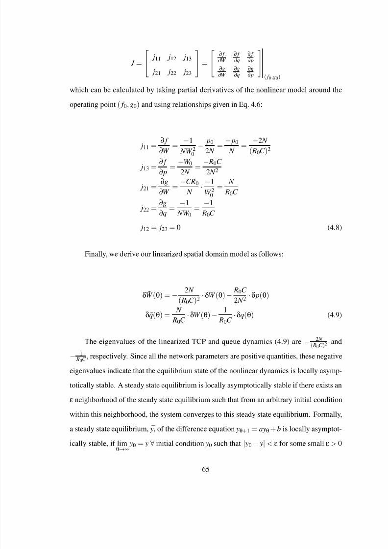
7/31/2019 Mehmet Tez
http://slidepdf.com/reader/full/mehmet-tez 75/95
J =
⎡⎣ j11 j12 j13
j21 j22 j23
⎤⎦=
⎡⎣ ∂ f
∂W ∂ f
∂q∂ f
∂ p
∂g
∂W ∂g
∂q∂g
∂ p
⎤⎦( f 0,g0)
which can be calculated by taking partial derivatives of the nonlinear model around the
operating point ( f 0, g0) and using relationships given in Eq. 4.6:
j11 =∂ f
∂W =
−1
NW 20−
p0
2 N =
− p0
N =
−2 N
( R0C )2
j13 =∂ f
∂ p=
−W 0
2 N =
− R0C
2 N 2
j21 =∂g
∂W =
−CR0
N
·−1
W 20=
N
R0C
j22 =∂g
∂q=
−1
NW 0=
−1
R0C
j12 = j23 = 0 (4.8)
Finally, we derive our linearized spatial domain model as follows:
δW (θ) = − 2 N
( R0C )2·δW (θ) − R0C
2 N 2·δ p(θ)
δq(θ) =N
R0C ·δW (θ) −
1
R0C ·δq(θ) (4.9)
The eigenvalues of the linearized TCP and queue dynamics (4.9) are − 2 N ( R0C )2 and
− 1 R0C , respectively. Since all the network parameters are positive quantities, these negative
eigenvalues indicate that the equilibrium state of the nonlinear dynamics is locally asymp-
totically stable. A steady state equilibrium is locally asymptotically stable if there exists an
ε neighborhood of the steady state equilibrium such that from an arbitrary initial condition
within this neighborhood, the system converges to this steady state equilibrium. Formally,
a steady state equilibrium, ¯ y, of the difference equation yθ+1 = ayθ+ b is locally asymptot-
ically stable, if limθ→∞
yθ = ¯ y ∀ initial condition y0 such that | y0 − ¯ y| < ε for some small ε > 0
65

7/31/2019 Mehmet Tez
http://slidepdf.com/reader/full/mehmet-tez 76/95
[14].
4.7 Event-Driven Congestion Controller Design
For event-driven congestion control, we implement a PI (Proportional and Integral)
controller to manage the drop probability for congestion control. A PI controller is a vari-
ation of a popular PID (Proportional, Integral and Differential) controller. A proportional
controller computes the control signal in proportion to the error, i.e., the difference be-
tween the measured performance of the controlled system and the specified reference per-
formance. A proportional controller by itself cannot support the stability of the feedback
control system [40]. An integrator is a low pass filter and it can support the stability of the
closed-loop system. In this chapter, an integrator is employed to allow traf fic bursts as dis-
cussed before, while supporting the stability of the closed-loop congestion control system.
We do not use a differential controller, because it may show unreliable performance when
workloads are highly dynamic. The time-driven congestion controller developed by Hollot
et al. [19] is also implemented using a PI controller.
We formulate the PI Controller as a transfer function, which characterizes the behavior
of a closed-loop system [40] in the discrete time z domain rather than in the continuous
time s domain, because most of computational systems, such as routers, usually work in
the discrete time domain. Further, the notation ˜ z is used instead of z in the following PI
transfer function to emphasize that the discretization has been made in the spatial domain,
instead of the time domain:
C ( z) =α(˜ z −β)
˜ z − 1(4.10)
where α= K P(K I +1), β = 1K I +1 . K P and K I are the proportional and integral control gains.
To tune the control gains, K P and K I , to support the stability of the closed-loop system
for AQM, we apply the Root Locus design method [40], in which one can graphically tune
feedback control gains. For more details about the Root Locus method, readers are referred
to [40].
66
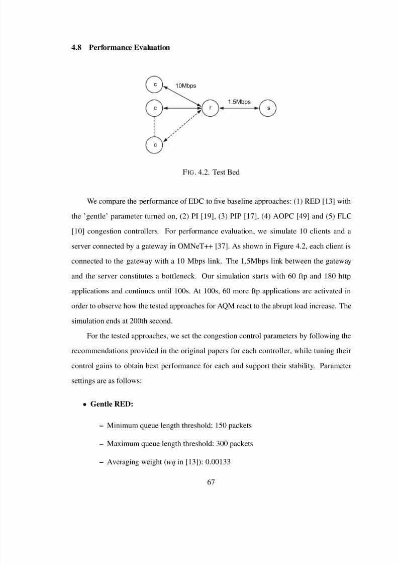
7/31/2019 Mehmet Tez
http://slidepdf.com/reader/full/mehmet-tez 77/95
4.8 Performance Evaluation
1.5Mbps
10Mbps
c r s
c
c
FIG. 4.2. Test Bed
We compare the performance of EDC to five baseline approaches: (1) RED [13] with
the ’gentle’ parameter turned on, (2) PI [19], (3) PIP [17], (4) AOPC [49] and (5) FLC
[10] congestion controllers. For performance evaluation, we simulate 10 clients and a
server connected by a gateway in OMNeT++ [37]. As shown in Figure 4.2, each client is
connected to the gateway with a 10 Mbps link. The 1.5Mbps link between the gateway
and the server constitutes a bottleneck. Our simulation starts with 60 ftp and 180 http
applications and continues until 100s. At 100s, 60 more ftp applications are activated in
order to observe how the tested approaches for AQM react to the abrupt load increase. The
simulation ends at 200th second.
For the tested approaches, we set the congestion control parameters by following the
recommendations provided in the original papers for each controller, while tuning their
control gains to obtain best performance for each and support their stability. Parameter
settings are as follows:
• Gentle RED:
– Minimum queue length threshold: 150 packets
– Maximum queue length threshold: 300 packets
– Averaging weight (wq in [13]): 0.00133
67

7/31/2019 Mehmet Tez
http://slidepdf.com/reader/full/mehmet-tez 78/95
– Maximum drop probability: 0.1
• PI Controller
– Reference (set-point) queue length: 200 packets
– Sampling frequency: 160 Hz (as recommended in [19])
– K P = 0.0015 and K I = 0.0003 (tuned via the Root Locus design method [40])
• PIP
– Reference queue length: 200 packets
– Sampling frequency: 160 Hz
– K h = 0.0021,τ = 0.47 (tuned via the Root Locus design method [40])
• AOPC
– Reference queue length: 200 packets
– Sampling frequency: 160 Hz
• FLC
– Reference queue length: 200 packets
– Sampling frequency: 160 Hz
– K e = 0.05 and K δe = 0.01 (tuned via trial and error)
• EDC:
– Reference queue length: 200 packets
– Event threshold: 30 packets
– K P = 0.03 and K I = 0.01 (tuned via the Root Locus design method [40])
For performance analysis, we show (1) the average and transient queue length, (2)
E2E delay, (3) number of packet drops and (4) controller activation frequencies. Since the
measured link utilization is almost 100% for all the tested approaches, we do not plot it.
68
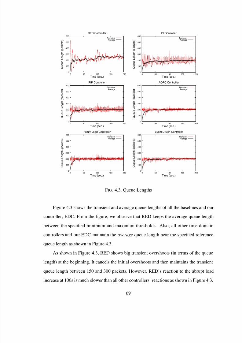
7/31/2019 Mehmet Tez
http://slidepdf.com/reader/full/mehmet-tez 79/95
0
100
200
300
400
500
600
0 50 100 150 200
Q u e u e L e n g t h ( p a c k e t s )
Time (sec.)
RED Controller
TransientAverage
0
100
200
300
400
500
600
0 50 100 150 200
Q u e u e L e n g t h ( p a c k e t s )
Time (sec.)
PI Controller
TransientAverage
0
100
200
300
400
500
600
0 50 100 150 200
Q u e u e L e n g t h ( p a c k e t s )
Time (sec.)
PIP Controller
TransientAverage
0
100
200
300
400
500
600
0 50 100 150 200
Q u e u e L e n g t h ( p a c k e t s )
Time (sec.)
AOPC Controller
TransientAverage
0
100
200
300
400
500
600
0 50 100 150 200
Q u e u e L e n g t h ( p a c k e t s )
Time (sec.)
Fuzzy Logic Controller
TransientAverage
0
100
200
300
400
500
600
0 50 100 150 200
Q u e u e L e n g t h ( p a c k e t s )
Time (sec.)
Event Driven Controller
TransientAverage
FIG. 4.3. Queue Lengths
Figure 4.3 shows the transient and average queue lengths of all the baselines and our
controller, EDC. From the figure, we observe that RED keeps the average queue length
between the specified minimum and maximum thresholds. Also, all other time domain
controllers and our EDC maintain the average queue length near the specified reference
queue length as shown in Figure 4.3.
As shown in Figure 4.3, RED shows big transient overshoots (in terms of the queue
length) at the beginning. It cancels the initial overshoots and then maintains the transient
queue length between 150 and 300 packets. However, RED’s reaction to the abrupt load
increase at 100s is much slower than all other controllers’ reactions as shown in Figure 4.3.
69
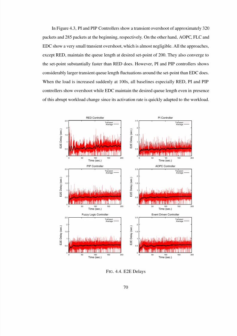
7/31/2019 Mehmet Tez
http://slidepdf.com/reader/full/mehmet-tez 80/95
In Figure 4.3, PI and PIP Controllers show a transient overshoot of approximately 320
packets and 285 packets at the beginning, respectively. On the other hand, AOPC, FLC and
EDC show a very small transient overshoot, which is almost negligible. All the approaches,
except RED, maintain the queue length at desired set-point of 200. They also converge to
the set-point substantially faster than RED does. However, PI and PIP controllers shows
considerably larger transient queue length fluctuations around the set-point than EDC does.
When the load is increased suddenly at 100s, all baselines especially RED, PI and PIP
controllers show overshoot while EDC maintain the desired queue length even in presence
of this abrupt workload change since its activation rate is quickly adapted to the workload.
0
0.5
1
1.5
2
2.5
0 50 100 150 200
E 2 E D e l a y ( s e c . )
Time (sec.)
RED Controller
TransientAverage
0
0.5
1
1.5
2
2.5
0 50 100 150 200
E 2 E D e l a y ( s e c . )
Time (sec.)
PI Controller
TransientAverage
0
0.5
1
1.5
2
2.5
0 50 100 150 200
E 2 E D e l a y ( s e c . )
Time (sec.)
PIP Controller
TransientAverage
0
0.5
1
1.5
2
2.5
0 50 100 150 200
E 2 E D e l a y ( s e c . )
Time (sec.)
AOPC Controller
TransientAverage
0
0.5
1
1.5
2
2.5
0 50 100 150 200
E 2 E D e l a y ( s e c . )
Time (sec.)
Fuzzy Logic Controller
TransientAverage
0
0.5
1
1.5
2
2.5
0 50 100 150 200
E 2 E D e l a y ( s e c . )
Time (sec.)
Event Driven Controller
TransientAverage
FIG. 4.4. E2E Delays
70
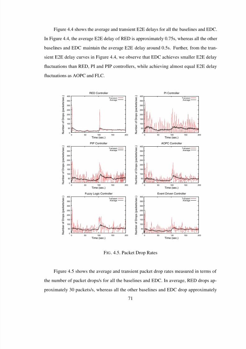
7/31/2019 Mehmet Tez
http://slidepdf.com/reader/full/mehmet-tez 81/95
Figure 4.4 shows the average and transient E2E delays for all the baselines and EDC.
In Figure 4.4, the average E2E delay of RED is approximately 0.75s, whereas all the other
baselines and EDC maintain the average E2E delay around 0.5s. Further, from the tran-
sient E2E delay curves in Figure 4.4, we observe that EDC achieves smaller E2E delay
fluctuations than RED, PI and PIP controllers, while achieving almost equal E2E delay
fluctuations as AOPC and FLC.
0
50
100
150
200
250
300
350
400
0 50 100 150 200 N u m b e r o f D r o p s ( p a c k e t s / s e c . )
Time (sec.)
RED Controller
TransientAverage
0
50
100
150
200
250
300
350
400
0 50 100 150 200 N u m b e r o f D r o p s ( p a c k e t s / s e c . )
Time (sec.)
PI Controller
TransientAverage
0
50
100
150
200
250
300
350
400
0 50 100 150 200 N
u m b e r o f D r o p s ( p a c k e t s / s e c . )
Time (sec.)
PIP Controller
TransientAverage
0
50
100
150
200
250
300
350
400
0 50 100 150 200 N
u m b e r o f D r o p s ( p a c k e t s / s e c . )
Time (sec.)
AOPC Controller
TransientAverage
0
50
100
150
200
250
300
350
400
0 50 100 150 200 N u m b e r o f D r o p s ( p a c k e t s / s e c . )
Time (sec.)
Fuzzy Logic Controller
TransientAverage
0
50
100
150
200
250
300
350
400
0 50 100 150 200 N u m b e r o f D r o p s ( p a c k e t s / s e c . )
Time (sec.)
Event Driven Controller
TransientAverage
FIG. 4.5. Packet Drop Rates
Figure 4.5 shows the average and transient packet drop rates measured in terms of
the number of packet drops/s for all the baselines and EDC. In average, RED drops ap-
proximately 30 packets/s, whereas all the other baselines and EDC drop approximately
71
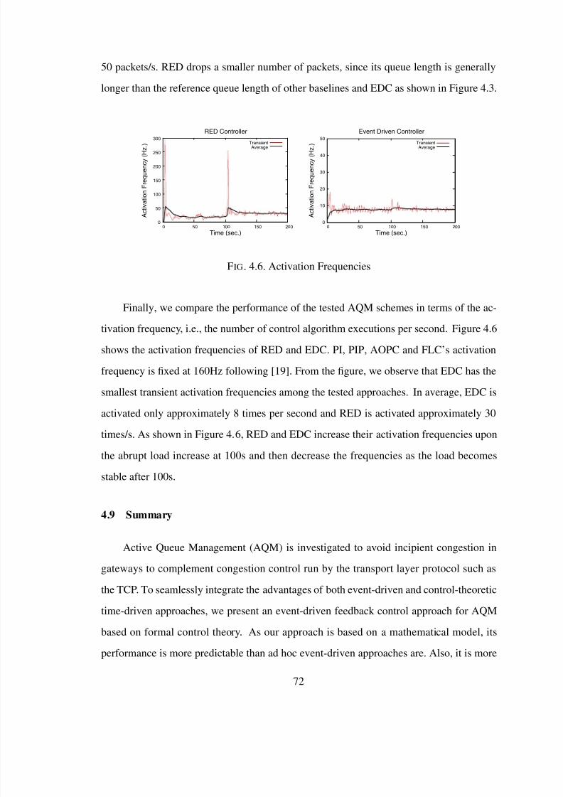
7/31/2019 Mehmet Tez
http://slidepdf.com/reader/full/mehmet-tez 82/95
50 packets/s. RED drops a smaller number of packets, since its queue length is generally
longer than the reference queue length of other baselines and EDC as shown in Figure 4.3.
0
50
100
150
200
250
300
0 50 100 150 200
A c t i v a t i o n F r e q u e n c y ( H z . )
Time (sec.)
RED Controller
TransientAverage
0
10
20
30
40
50
0 50 100 150 200
A c t i v a t i o n F r e q u e n c y ( H z . )
Time (sec.)
Event Driven Controller
TransientAverage
FIG. 4.6. Activation Frequencies
Finally, we compare the performance of the tested AQM schemes in terms of the ac-
tivation frequency, i.e., the number of control algorithm executions per second. Figure 4.6
shows the activation frequencies of RED and EDC. PI, PIP, AOPC and FLC’s activation
frequency is fixed at 160Hz following [19]. From the figure, we observe that EDC has the
smallest transient activation frequencies among the tested approaches. In average, EDC is
activated only approximately 8 times per second and RED is activated approximately 30times/s. As shown in Figure 4.6, RED and EDC increase their activation frequencies upon
the abrupt load increase at 100s and then decrease the frequencies as the load becomes
stable after 100s.
4.9 Summary
Active Queue Management (AQM) is investigated to avoid incipient congestion in
gateways to complement congestion control run by the transport layer protocol such as
the TCP. To seamlessly integrate the advantages of both event-driven and control-theoretic
time-driven approaches, we present an event-driven feedback control approach for AQM
based on formal control theory. As our approach is based on a mathematical model, its
performance is more predictable than ad hoc event-driven approaches are. Also, it is more
72

7/31/2019 Mehmet Tez
http://slidepdf.com/reader/full/mehmet-tez 83/95
reactive to dynamic load changes than time-driven approaches due to its even-driven na-
ture. We analyze the stability of the open-loop model and tune the event-driven controller
to support the stability of the closed loop system by applying formal control theoretic tech-
niques. Our simulation results show that our event-driven controller effectively maintains
the queue length around the specified set-point. It generally achieves shorter E2E (end-
to-end) delays and smaller E2E delay fluctuations than the baselines. Further, our AQM
algorithm is invoked much less frequently than the tested baselines. In the future, we will
continue to investigate more cost-effective approaches for active queue management.
73
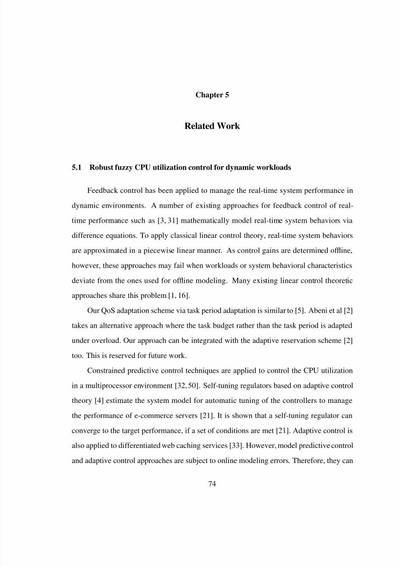
7/31/2019 Mehmet Tez
http://slidepdf.com/reader/full/mehmet-tez 84/95
Chapter 5
Related Work
5.1 Robust fuzzy CPU utilization control for dynamic workloads
Feedback control has been applied to manage the real-time system performance in
dynamic environments. A number of existing approaches for feedback control of real-
time performance such as [3, 31] mathematically model real-time system behaviors via
difference equations. To apply classical linear control theory, real-time system behaviors
are approximated in a piecewise linear manner. As control gains are determined of fline,
however, these approaches may fail when workloads or system behavioral characteristics
deviate from the ones used for of fline modeling. Many existing linear control theoretic
approaches share this problem [1, 16].Our QoS adaptation scheme via task period adaptation is similar to [5]. Abeni et al [2]
takes an alternative approach where the task budget rather than the task period is adapted
under overload. Our approach can be integrated with the adaptive reservation scheme [2]
too. This is reserved for future work.
Constrained predictive control techniques are applied to control the CPU utilization
in a multiprocessor environment [32,50]. Self-tuning regulators based on adaptive control
theory [4] estimate the system model for automatic tuning of the controllers to manage
the performance of e-commerce servers [21]. It is shown that a self-tuning regulator can
converge to the target performance, if a set of conditions are met [21]. Adaptive control is
also applied to differentiated web caching services [33]. However, model predictive control
and adaptive control approaches are subject to online modeling errors. Therefore, they can
74
7/31/2019 Mehmet Tez
http://slidepdf.com/reader/full/mehmet-tez 85/95
only handle moderate nonlinearity. In contrast, fuzzy logic control is very effective to
manage the performance of nonlinear, complex systems due to the model-free nature [39].
Fuzzy control theory has been applied to maximize the profit in an e-mail server [7].
eQoS [54] applies fuzzy control theory to differentiate services in a web server. However,
they do not consider real-time constraints.
Little prior work has been done to apply fuzzy control theory to real-time perfor-
mance management. Li et al [26] apply fuzzy control to visual tracking; however, they
do not consider the utilization control problem. Further, they do not analyze the stability
of the fuzzy closed-loop system. Suzer et al [45] have developed a fuzzy utilization con-
troller. However, this study presents a more advanced fuzzy rule-base to reduce potential
overshoots and undershoots. Further, [45] does not provide stability analysis and evaluates
performance via simulation.
5.2 Bandwidth Consumption Control and Service Differentiation for Video Stream-
ing
Our bit rate management and service differentiation schemes are implemented atop
QStream [25]. QStream supports real-time video streaming by EDF (earliest deadline first)
scheduling of frames based on their playtime deadlines and synchronization between the
client and server. qVSF significantly extends QStream to support the specified bandwidth
limit and service differentiation.
A fuzzy controller [24] determines the emitted QoS level of video streams. The error
value fed into the fuzzy controller is the difference between the stream quality emitted from
the server and the stream quality perceived at the client. They aim to find the point where
the difference between the emitted QoS level and the perceived one is zero. However, bit
rate control and service differentiation are not considered in their work.
A fuzzy logic based cross-layer video streaming solution for wireless media is pre-
sented in [47]. The feedback is received from the underlying network stack to change the
bit rate of a video according to link conditions. However, their work only considers a single
75
7/31/2019 Mehmet Tez
http://slidepdf.com/reader/full/mehmet-tez 86/95
7/31/2019 Mehmet Tez
http://slidepdf.com/reader/full/mehmet-tez 87/95
trol algorithm execution for congestion control. Unlike these approaches, our work is not
only event-driven but also based on formal control theoretic techniques. We discuss a few
representative existing approaches from the two camps that are closely related to our work
in the following.
Ad Hoc Event-Driven Approaches. RED [13] controls the queue length by monitoring
the average queue length and manipulating the packet drop/mark probability, if necessary,
to avoid congestion. Although RED is very effective, it has several parameters to tune.
Further, tuning is not always straightforward. Lin et al. proposed Flow Random Early
Drop (FRED) [27]. They evaluate the effectiveness of RED over traf fic types categorized
as nonadaptive, fragile and robust, according to their responses to congestion. They point
out that RED allows unfair bandwidth sharing when a mixture of the three traf fic types
shares a link. FRED uses per-active-flow accounting to impose on each flow a loss rate
that depends on the flow?s buffer use. Ott et al. proposed Stabilized RED (SRED) [38]
to statistically estimate the number of active flows at a link and also identify misbehaving
flows. SRED uses the estimated number of active flows and the instantaneous queue size to
calculate the packet-dropping probability. Feng et al. developed a self-configuring version
of RED [9]. The authors suggest using an on-line algorithm for dynamically changing
RED parameters according to the observed traf fic. The authors show that this mechanism
can reduce packet losses, while maintaining high link utilization. Feng et al. proposed
BLUE [8] as a congestion control algorithm to be deployed in gateways. By considering
packet loss and link idle events to manage congestion, BLUE significantly outperformed
RED.
Time-Driven Feedback Control Approaches. Misra et al. modeled the interactions of
TCPfl
ows and AQM routers by using stochastic differential equations [35]. Using thismodel in their simulations, they analyzed the impact of RED parameters on the network
performance. This mathematical model constitutes a basis for a number of projects re-
garding AQM. The authors of [19], [56], [17], [49] and [10] used this model to develop
control-theoretic approaches for AQM. Hollot et al. analyzed RED in control theoretic as-
pects [18] using the mathematical model developed in [35]. Using this model, they also
77

7/31/2019 Mehmet Tez
http://slidepdf.com/reader/full/mehmet-tez 88/95
developed a P and a PI controller in a companion paper [19]. Zhang et al. proposed an
online self-tuning structure [56] based on the mathematical model [35] to estimate and
correct network parameters online. Accompanied by a PI controller, this structure is used
to manage the queue length. Heying et al. [17] developed a novel algorithm, called Pro-
portional Integral based series compensation and Position feedback compensation (PIP),
to manage the queue length. They used the model developed in [35] to implement their
approach. Wang et al. [49] proposed an optimized version of the mathematical model in
[35] and they built the Adaptive Optimized Proportional Controller (AOPC). AOPC mea-
sures the latest packet loss ratio and uses it as a complement to the queue length in order to
dynamically adjust the packet drop probability. It measures an additional state information,
i.e., latest packet loss ratio, to enhance the control performance. Fengyuan et al. [10] built
a fuzzy logic controller based on the model developed by Misra et al. [35] to manage the
queue length. Their approach is inspired by the fact that fuzzy control theory [39] is more
versatile than the classical control theoretical solutions in the presence of nonlinear system
behaviors. However, their approach is also time-driven.
78
7/31/2019 Mehmet Tez
http://slidepdf.com/reader/full/mehmet-tez 89/95
Chapter 6
Conclusions and Future Work
Computer systems have limited amounts of resources to serve applications’ growing
demands. Most systems tend to allocate resources to applications by of fline analysis of ap-
plication requirements, which often results in inef ficient resource usage due to the dynamic,
time-varying nature of workloads. Formal control theory is known to effectively support
the desired performance of the controlled system. However, it is challenging to support the
performance of computational systems, since there is no definitive methodology to model
computer system dynamics unlike physics laws applied to model physical systems such
as a cruise control system. Modeling computer systems, selecting proper control theoretic
tools and tuning them according to the needs of specific applications-the research problems
to be investigated in this proposed work-are the key ingredients for successful application
of control theory to computer system performance management. To support desired system
performance even in the presence of dynamic workloads, we have applied advanced con-
trol theoretic approaches, namely fuzzy control theory, model predictive control theory and
event-driven control theoretic techniques. Specifically, we apply these techniques to man-
age the CPU utilization in a real-time operating system, network bandwidth consumption
for video streaming, and link congestion in network gateways.
First, to reduce the dif ficulty of modeling real-time systems with stringent timing con-
straints, we apply formal fuzzy control theory that is very effective to support the desired
performance in a nonlinear dynamic system without requiring a system model. We sup-
port direct nonlinear mappings between the utilization error (= target utilization − current
utilization) and the workload adjustment required to achieve the target utilization via IF-
79
7/31/2019 Mehmet Tez
http://slidepdf.com/reader/full/mehmet-tez 90/95
THEN rules. Rather than relying on an approximate system model, we develop a novel
fuzzy closed-loop system to control the utilization based on the logical understanding of
the relation between the workload and utilization changes. Via the Lyapunov direct method
[4, 39], we mathematically prove the stability of the fuzzy closed-loop system. Further, we
extend the Real-Time Application Interface (RTAI) for Linux kernel [43]. We implement
and evaluate our fuzzy logic utilization controller as well as two existing utilization con-
trollers based on the linear and model predictive control theory for an extensive set of
workloads in RTAI. Among the tested approaches, our approach shows the smallest devia-
tion from and the fastest convergence to the specified utilization set-point when the system
is in a transient status.
Second, we applied fuzzy control theory to network bandwidth consumed by multi-
media streaming. In this way, we aim to avoid undesirable situations in which multimedia
streaming starves other applications such as file transfer sharing the network, for example,
in a smart home. To bound the bandwidth usage of streaming, we leverage the layered en-
coding technique, in which a video frame consists of a base layer and multiple enhancement
layers. We always transmit the base layer, because it is required to display a scene. How-
ever, under overload, we degrade the video quality by dropping high enhancement layers
without affecting the underlying layers, if necessary, to support the specified bit rate bound.
We have implemented our transmission rate control and service differentiation schemes on
top of an open source video streaming server, QStream [42] and evaluated by running ex-
periments across the shared department network in the Department of Computer Science at
SUNY Binghamton where a considerable number of different applications usually coexist
at the same time. Performance evaluation results show that our video streaming system
can support the specifi
ed bit rate bound and differentiate the service to ef fi
ciently utilizethe limited bandwidth without severely degrading the visual quality of low priority video
streams.
Third, we applied formal event-driven control theory to address the congestion control
problem in gateways. Most existing work on AQM is either ad-hoc event-driven feedback
approaches or time-driven formal control theoretic approaches. To integrate the advantages
80
7/31/2019 Mehmet Tez
http://slidepdf.com/reader/full/mehmet-tez 91/95
of both event-driven and time-driven control-theoretic approaches, we present an event-
driven feedback control approach based on formal control theory [15, 40]. The key idea of
our approach is to design a feedback-based congestion controller that is invoked upon the
arrivals of a specified number of packets rather than being invoked at every fixed sampling
period. As our approach is based on a mathematical model, its performance is easier to
analyze and more predictable than ad-hoc event-driven approaches are.
We thoroughly evaluate the performance of our approach via an extensive simulation
study in OMNeT++ [37]. We compare it to five advanced approaches for AQM. Our sim-
ulation results show that our event-driven controller effectively maintains the queue length
around the specified set-point. It achieves shorter E2E (end-to-end) delays and smaller E2E
delay fluctuations than several existing AQM approaches while achieving almost the same
E2E delays and E2E delay fluctuations as the two other advanced control theoretic AQM
approaches. Further, our AQM algorithm is invoked much less frequently than the tested
baselines. Therefore, it saves precious resources at routers.
In summary, I aim to demonstrate the applicability of formal control theoretic tech-
niques to support desired system behaviors even in the presence of dynamic workloads
and uncertain environments. In this way, I intend to improve the predictability and reli-
ability of computer systems that need to process highly dynamic workloads in uncertain
environments.
81
7/31/2019 Mehmet Tez
http://slidepdf.com/reader/full/mehmet-tez 92/95
References
[1] T. F. Abdelzaher, J. A. Stankovic, C. Lu, R. Zhang, and Y. Lu. Feedback Performance Controlin Software Services. IEEE Control Systems Magazine, 23(3), 2003.
[2] L. Abeni, T. Cucinotta, G. Lipari, L. Marzario, and L. Palopoli. QoS Management ThroughAdaptive Reservations. Real-Time Systems, 29(2-3), 2005.
[3] M. Amirijoo, J. Hansson, S. H. Son, and S. Gunnarsson. Experimental Evaluation of LinearTime-Invariant Models for Feedback Performance Control in Real-Time System. In Real-
Time Systems, volume 35, 2007.
[4] K. J. Astrom and B. Wittenmark. Adaptive Control. Addison-Wesley, 2nd edition, 1994.
[5] G. Buttazzo, G. Lipari, and L. Abeni. Elastic Task Model For Adaptive Rate Control. In IEEE
Real-Time Systems Symposium, 1998.
[6] R. Carlson. Sandia SCADA Program High-Security SCADA LDRD Final Report. Technicalreport, SANDIA, 2002. SANDIA Report SAND2002-0729.
[7] Y. Diao, J. L. Hellerstein, and S. Parekh. Using Fuzzy Control to Maximize Profits in ServiceLevel Management. IBM Systems Journal, 41(3), 2002.
[8] W. Feng, D. Kandlur, D. Saha, and K. Shin. The Blue active queue management algorithms. IEEE/ACM Transactions on Networking, 10(4):513–528, 2002.
[9] W. Feng, D. D. Kandlur, D. Saha, and K. G. Shin. A self-configuring RED gateway. In INFOCOM , 1999.
[10] R. Fengyuan, R. Yong, and S. Xiuming. Design of a fuzzy controller for active queue man-agement. Computer Communication, 1(25):874–883, 2002.
[11] S. Floyd. Recommendations on using the gentle variant of RED, 2000. Available atwww.icir.org/ floyd/red/gentle.html.
[12] S. Floyd, R. Gummadi, and S. Shenker. Adaptive RED: An algorithm for in-creasing the robustness of REDs active queue management, 2001. Available athttp://www.icir.org/ floyd/papers/adaptiveRed.pdf.
[13] S. Floyd and V. Jacobson. Random early detection gateways for congestion avoidance. IEEE/ACM Transactions on Networking, 1(4):397–413, 1993.
[14] O. Galor. Discrete Dynamical Systems. Springer, 2007.
[15] W. Heemels, R. Gorter, A. van Zijl, P. van den Bosch, S. Weiland, W. Hendrix, and M. Vonder.Asynchronous measurement and control: A case study on motor synchronization. Elsevier
Control Engineering Practice, 7(12):1467–1482, 1999.
[16] J. L. Hellerstein, Y. Diao, S. Parekh, and D. M. Tilbury. Feedback Control of Computing
Systems. A John Wiley and Sons, Inc., Publication, 2004.
82
7/31/2019 Mehmet Tez
http://slidepdf.com/reader/full/mehmet-tez 93/95
[17] Z. Heying, L. Baohong, and D. Wenhua. Design of a robust active queue management algo-rithm based on feedback compensation. In SIGCOMM , 2003.
[18] C. Hollot, V. Misra, D. Towsley, and W. B. Gong. A control theoretic analysis of RED. In INFOCOM , 2001.
[19] C. Hollot, V. Misra, D. Towsley, and W. B. Gong. On designing improved controllers forAQM routers supporting TCP flows. In INFOCOM , 2001.
[20] V. Jacobson. Congestion avoidance and control. In ACM SIGCOMM , 1988.
[21] C. Karamanolis, M. Karlsson, and X. Zhu. Designing Controllable Computer Systems. InUSENIX Workshop on Hot Topics in Operating Systems, 2005.
[22] M. Karlsson and M. Covell. Dynamic black-box performance model estimation for self-tuningregulators. In International Conference on Autonomic Computing, 2005.
[23] G. Klir and B. Yuan. Fuzzy Sets and Fuzzy Logic: Theory and Applications. Prentice Hall,1995.
[24] C. Koliver, K. Nahrstedt, J.-M. Farines, J. da Silva Fraga, and S. A. Sandri. Specification,Mapping and Control for QoS Adaptation. Real-Time Systems, 23(1-2):143–174, 2002.
[25] C. Krasic, J. Walpole, and W.-C. Feng. Quality-Adaptive Media Streaming by Priority Drop.In NOSSDAV ’03, 2003.
[26] B. Li and K. Nahrstedt. A Control-Based Middleware Framework for Quality of ServiceAdaptations. IEEE Journal on Selected Areas in Communications, 17(9), 1999.
[27] D. Lin and R. Morris. Dynamics of random early detection. In SIGCOMM , 1997.
[28] K. J. Lin, S. Natarajan, and J. W. S. Liu. Imprecise Results: Utilizing Partial Computations inReal-Time Systems. In Real-Time System Symposium, December 1987.
[29] J. W. S. Liu. Real-Time Systems. Prentice Hall, 2000.
[30] J. Loyall, R. Schantz, D. Corman, and J. P. andS. Fernandez. A Distributed Real-Time Em-bedded Application for Surveillance, Detection, and Tracking of Time Critical Targets. In The
11th IEEE Real-Time Embedded Technology and Applications Symposium, 2005.
[31] C. Lu, J. A. Stankovic, G. Tao, and S. H. Son. Feedback Control Real-Time Schedul-ing: Framework, Modeling and Algorithms. Real-Time Systems, Special Issue on Control-
Theoretical Approaches to Real-Time Computing, 23(1/2), May 2002.
[32] C. Lu, X. Wang, and X. Koutsoukos. Feedback Utilization Control in Distributed Real-TimeSystems with End-to-End Tasks. IEEE Transactions on Parallel and Distributed Systems,16(6):550–561, June 2005.
[33] Y. Lu, A. Saxena, and T. F. Abdelzaher. Differentiated Caching Services; A Control-Theoretical Approach. In International Conference on Distributed Computing Systems, 2002.
[34] J. Maciejowski. Predictive Control with Constraints. Prentice Hall, 2002.
83
7/31/2019 Mehmet Tez
http://slidepdf.com/reader/full/mehmet-tez 94/95
[35] V. Misra, W. B. Gong, and D. Towsley. Fluid-based analysis of a network of AQM routerssupporting TCP flows with an application to red. In SIGCOMM , 2000.
[36] R. K. Mudi and N. R. Pal. A Self-Tuning Fuzzy PI Controller. Fuzzy Sets and Systems,115(2):327–338, October 2000.
[37] OMNET++ - A discrete event simulation environment. http://www.omnetpp.org.
[38] T. J. Ott, T. V. Lakshman, and L. H.Wong. SRED: Stabilized red. In INFOCOM , 1999.
[39] K. M. Passino and S. Yurkovich. Fuzzy Control. Addison-Wesley, 1998.
[40] C. Phillips and H. Nagle. Digital Control System Analysis and Design. Prentice Hall, 1995.
[41] C. L. Phillips and H. T. Nagle. Digital Control System Analysis and Design (3rd edition).Prentice Hall, 1995.
[42] QStream Home. http://qstream.org.
[43] RTAI - The RealTime Application Interface for Linux from DIAPM. http://www.rtai.org.
[44] J. Sun, K.-T. Ko, G. Chen, S. Chan, and M. Zukerman. Pd-red: to improve the performanceof red. Communications Letters, IEEE , 7(8):406 – 408, 2003.
[45] M. H. Suzer and K. D. Kang. Adaptive Fuzzy Control for Utilization Management. In IEEE
International Symposium on Object/component/service-oriented Real-time distributed Com-
puting, 2008.
[46] P. van der Stok, D. Jarnikov, S. Kozlov, M. van Hartskamp, and J. J. Lukkien. HierarchicalResource Allocation for Robust In-Home Video Streaming. Journal of Systems and Software,80(7):951–961, 2007.
[47] J. Vehkapera, M. Myllyniemi, and J. Peltola. Fuzzy Logic-Based Cross-Layer Controller forScalable Video Streaming. In IMSA’07 , 2007.
[48] Z. Vukic. Nonlinear Control Systems. Marcel Dekker, 2003.
[49] J. Wang, L. Rong, and Y. Liu. A robust proportional controller for AQM based on optimized2nd order system model. Computer Communication, 1(31):2468–2477, 2008.
[50] X. Wang, D. Jia, C. Lu, and X. Koutsoukos. DEUCON: Decentralized End-to-End UtilizationControl for Distributed Real-Time Systems. IEEE Transactions on Parallel and Distributed
Systems, 18(7):996–1009, July 2007.
[51] X. Wang, D. Jia, C. Lu, and X. Koutsoukos. DEUCON: Decentralized End-to-End UtilizationControl for Distributed Real-Time Systems. IEEE Transactions on Parallel and Distributed
Systems, 18(7):996–1009, 2007.
[52] X. Wang, C. Lu, and C. Gill. FCS/nORB: A Feedback Control Real-Time Scheduling Servicefor Embedded ORB Middleware. Microprocessors and Microsystems, 32(8):413–424, Nov.2008.
84
7/31/2019 Mehmet Tez
http://slidepdf.com/reader/full/mehmet-tez 95/95