Embed Size (px)
Citation preview
P R O J E C T
MERRByS
MERRByS Product Manual - GNSS Reflectometry on TDS-1 with the SGR-ReSI
W O R K P A C K A G E N U M B E R
SS E P
S S T L R E F E R E N C E
0248366
R E V I S I O N
003
R E V I S I O N O R R E L E A S E D A T E
19/07/2017
S T A T U S
Released
Surrey Satellite Technology Limited Tycho House 20 Stephenson Road Surrey Research Park Guildford, Surrey GU2 7YE, UK Tel: +44 1483 803803 Fax: +44 1483 803804 Email: [email protected]
THIS DOCUMENT IS THE PROPERTY OF SURREY SATELLITE TECHNOLOGY LIMITED AND MUST NOT BE COPIED OR USED FOR ANY PURPOSE OTHER THAN THAT FOR WHICH IT HAS BEEN SUPPLIED.

MERRByS Product Manual - GNSS Reflectometry on TDS-1 with the SGR-
ReSI
Doc No: XP X H - #0248366
Revision: 003 Status: Released
Revision Release Date: 19/07/2017
Page 2 of 73
TABLE OF CONTENTS
1 INTRODUCTION ........................................................................................................................................ 8
1.1 SCOPE .................................................................................................................................................. 8
1.2 REFERENCE DOCUMENTS ................................................................................................................ 8
1.3 ACRONYMS AND ABBREVIATIONS ................................................................................................... 8
2 OVERVIEW 10
2.1 GNSS-R ............................................................................................................................................... 10
3 TECHDEMOSAT-1 GNSS-R EXPERIMENT ........................................................................................... 10
3.1 THE SGR-RESI ................................................................................................................................... 11
4 DATA ACCESS POLICY ......................................................................................................................... 13
4.1 LICENCE ............................................................................................................................................. 13
4.2 DATA SETS......................................................................................................................................... 13
5 DATA OVERVIEW ................................................................................................................................... 14
5.1 PRODUCT DEFINITIONS ................................................................................................................... 14
5.1.1 Differences of TDS-1 from CYGNSS Products ............................................................................. 16
6 L0 – RAW COLLECTIONS ...................................................................................................................... 17
7 L1A - ONBOARD PROCESSING ............................................................................................................ 18
7.1 SGR-RESI PROCESSING FUNCTIONS ............................................................................................ 18
7.1.1 Reflection Tracking ....................................................................................................................... 18
7.1.2 DDM Processing (The ZTC) .......................................................................................................... 19
7.1.3 Receiver operations ...................................................................................................................... 23
8 L0 AND L1A DATA TYPES FROM SPACECRAFT ............................................................................... 25
8.1 SBPP ................................................................................................................................................... 25
8.2 HSI ....................................................................................................................................................... 25
8.2.1 Level 0 (Raw) Data Format ........................................................................................................... 25
8.2.2 Level 1a (ZTC) Data -DDMs ......................................................................................................... 26
9 L0 TO L1B(SW) GROUND PROCESSED DDMS ................................................................................... 28
10 L1A TO L1B – DDM SYNCHRONISATION AND CALIBRATION ......................................................... 30
10.1 MERRBYS DATA SEGMENTATION .................................................................................................. 30
10.2 CATALOGUE ...................................................................................................................................... 32
11 L1B TO L2 – GEOPHYSICAL RETRIEVAL ............................................................................................ 33
11.1 CATALOGUE ...................................................................................................................................... 33
12 DATA FILE DEFINITIONS ....................................................................................................................... 34
12.1 FORMAT ............................................................................................................................................. 34
12.2 COMMON DEFINITIONS .................................................................................................................... 34
12.2.1 Time format ................................................................................................................................... 34
12.3 L0 TRACK SEARCH RAW COLLECTION FILE ................................................................................. 34

MERRByS Product Manual - GNSS Reflectometry on TDS-1 with the SGR-
ReSI
Doc No: XP X H - #0248366
Revision: 003 Status: Released
Revision Release Date: 19/07/2017
Page 3 of 73
© SSTL RELEASE VERSION
12.3.1 Structure: ....................................................................................................................................... 34
12.4 L0 RAW COLLECTION FILES ............................................................................................................ 36
12.5 L1B METADATA ................................................................................................................................. 36
12.5.1 Structure ........................................................................................................................................ 36
12.5.2 Attributes ....................................................................................................................................... 37
12.5.3 Variables ....................................................................................................................................... 37
12.5.4 Track Groups................................................................................................................................. 39
12.6 L1B DDM FILE .................................................................................................................................... 45
12.6.1 Structure ........................................................................................................................................ 45
12.6.2 Attributes ....................................................................................................................................... 45
12.6.3 Track Groups................................................................................................................................. 45
12.7 L1B BLACKBODY FILES .................................................................................................................... 46
12.7.1 Attributes ....................................................................................................................................... 46
12.7.2 Variables ....................................................................................................................................... 46
12.8 L1B DIRECT SIGNAL FILES .............................................................................................................. 47
12.8.1 Attributes ....................................................................................................................................... 47
12.8.2 Variables ....................................................................................................................................... 47
12.9 ANTENNA GAIN MAP FILE ................................................................................................................ 47
12.9.1 Structure ........................................................................................................................................ 47
12.9.2 Contents ........................................................................................................................................ 47
12.10 L2DATAFILE ....................................................................................................................................... 48
12.10.1 Structure ........................................................................................................................................ 48
12.10.2 Attributes ....................................................................................................................................... 48
12.10.3 Variables ....................................................................................................................................... 48
13 PROCESSING REFERENCE .................................................................................................................. 49
13.1 SPECULAR POINT LOCATION.......................................................................................................... 49
13.2 SATELLITE ATTITUDE AND ANTENNA GAIN .................................................................................. 50
13.2.1 Attitude reference frames .............................................................................................................. 50
13.2.2 Attitude representations ................................................................................................................ 51
13.2.3 Antenna Reference Frame ............................................................................................................ 52
13.3 DELAY DOPPLER MAP ...................................................................................................................... 53
13.3.1 DDM Scale .................................................................................................................................... 53
13.4 ADC METRICS .................................................................................................................................... 54
13.5 ANTENNA NOISE ESTIMATION ........................................................................................................ 55
14 L1B RADIOMETRIC CALIBRATION ...................................................................................................... 60
14.1.1 Radiometric Measurement Definitions .......................................................................................... 60
14.1.2 Receiver Measurements ............................................................................................................... 61
14.1.3 Derived Measurements ................................................................................................................. 61
14.1.4 Implementation Loss Terms .......................................................................................................... 67
15 RELEASE NOTES ................................................................................................................................... 68
15.1 RELEASE NOTES FOR L1B V0.5 ...................................................................................................... 68
15.1.1 Changes from v0.3 to v0.5 ............................................................................................................ 68
15.1.2 Changes from v0.5 to v0.7 ............................................................................................................ 69
NOC CONTRIBUTION TO TN3 “GROUND PROCESSING DESIGN” .......................................................... 71

MERRByS Product Manual - GNSS Reflectometry on TDS-1 with the SGR-
ReSI
Doc No: XP X H - #0248366
Revision: 003 Status: Released
Revision Release Date: 19/07/2017
Page 4 of 73
© SSTL RELEASE VERSION
A.1 INTRODUCTION ........................................................................................................................................ 71
A.2 NOC-FDI: ALGORITHM THEORETICAL BASIS ..................................................................................... 71
A.3 NOC-FDI: SOFTWARE DESCRIPTION .................................................................................................... 71
A.3.1 DDM PRE-PROCESSING ................................................................................................................... 71
A.3.2 SNR COMPUTATION ......................................................................................................................... 72
A.3.3 WIND SPEED AND MSS COMPUTATION ......................................................................................... 73
LIST OF FIGURES
Figure 2-1 GNSS-R Geometry ........................................................................................................................ 10 Figure 3-1 TechDemoSat-1 and GNSS-R Unit (part of SSP).......................................................................... 11 Figure 3-2 GNSS-R Instrument architecture .................................................................................................... 11 Figure 3-3 GPS L1 signal DDMs. Direct (Left) and Reflected from the ocean (Right). (Shown to the same scale) .......................................................................................................................................................................... 12 Figure 3-4 A sample of a DDM track of ocean reflections processed by the SGR-ReSI on TDS-1 ................ 12 Figure 5-1 Definition of TDS-1 GNSS-R Data Products .................................................................................. 14 Figure 6-1 Raw collection data flow within the SGR-ReSI ............................................................................... 17 Figure 7-1 Schematic representation of the GNSS-R DDM processing flow. Bold boxes indicate focus of this section............................................................................................................................................................... 18 Figure 7-2 Computation of DDM row through process of down-conversion, modulation removal followed by spectrum estimation .......................................................................................................................................... 20 Figure 7-3 Moving average filter ....................................................................................................................... 21 Figure 7-4 The CIC filter response showing post-decimation aliasing. ........................................................... 21 Figure 7-5 Aliasing into the required-band (green) ........................................................................................... 22 Figure 7-6: Switching operation of load a) DDM Mode (programmable gain), b) Raw data Collection mode . 24 Figure 8-1 GNSS-R data types from the spacecraft ......................................................................................... 25 Figure 8-2: Raw Data File Structure ................................................................................................................. 26 Figure 8-3: DDM file format components .......................................................................................................... 26 Figure 8-4: Example DDM file with 4 ZTC channels ........................................................................................ 27 Figure 9-1 Creation of L0 data from receiver outputs ....................................................................................... 28 Figure 9-2 Processing L0 to L1a DDMs using software receiver ..................................................................... 29 Figure 10-1 L1a to L1b processing flow ........................................................................................................... 31 Figure 11-1 Initial L1b to L2(Fast Delivery) Processing flow for geophysical retrieval ..................................... 33 Figure 13-1 Quasi-spherical approximation for determining the specular point location ................................ 49 Figure 13-2 Coordinate system definition ......................................................................................................... 51 Figure 13.3 Typical DDMs processed (Left) over the ocean (Right) over land. The red box corresponds to the region for estimating the antenna noise using a ‘Noise Box’............................................................................ 55 Figure 13.4 Specular point delay reduction due to topography ........................................................................ 56 Figure 13.5 The affect before and after dilation on a 1 pixel-wide Hawaiian volcano, Mauna Loa. ................. 57 Figure 13.6 Topographic map overlaid onto Google Earth optical imagery ..................................................... 57 Figure 13.7 Topographic map over South America (Left) Original map. (Right) Dilation of map ..................... 58 Figure 13.8 Overview of example track location (RD84, Track 4) .................................................................... 58 Figure 13.9 Example track showing a number of the features within one track (RD84, Track 4) ................... 59 Figure 14.1 Forward model of the received signal power through the simplified receiver chain ..................... 60 Figure 14.2 Flow of radiometric data from L1a DDMs to L1b DDMs ............................................................... 66 Figure 33: NOC-FDI function interface, input and output ................................................................................. 71 Figure 4: Illustration of the robust peak detection procedure and of the DDM regions used for the computation of Signal power (S) and Noise power (N) ............................................................................................................. 72
LIST OF TABLES
Table 5-1 Data Product Description ................................................................................................................ 15 Table 5-2 Data Product Differences Between TDS-1 and CYGNSS .............................................................. 16 Table 6-1 Nominal raw collection configuration ................................................................................................ 17

MERRByS Product Manual - GNSS Reflectometry on TDS-1 with the SGR-
ReSI
Doc No: XP X H - #0248366
Revision: 003 Status: Released
Revision Release Date: 19/07/2017
Page 5 of 73
© SSTL RELEASE VERSION
Table 7-1 Nominal Configuration of ZTC processor ......................................................................................... 22 Table 9-1 Software receiver configurations ...................................................................................................... 29 Table 10-1 Data segmentation times ................................................................................................................ 30 Table 0-1: DDM pre-processing parameters, naming and numerical values for UK-DMC. ............................. 72 Table 0-2: SNR computation parameters, naming and numerical values for UK-DMC. .................................. 73 Table 0-3: Output parameters .......................................................................................................................... 73

MERRByS Product Manual - GNSS Reflectometry on TDS-1 with the SGR-
ReSI
Doc No: XP X H - #0248366
Revision: 003 Status: Released
Revision Release Date: 19/07/2017
Page 6 of 73
© SSTL RELEASE VERSION
COPYRIGHT
COPYRIGHT AND LICENCE CONDITIONS
©SSTL THE COPYRIGHT IN THIS DOCUMENT IS THE PROPERTY OF SURREY SATELLITE TECHNOLOGY LIMITED. All rights reserved. No part of this documentation may be reproduced by any means in any material form (including photocopying or storing it in any electronic form) without the consent of the Copyright Owner, except in accordance with the Copyright, Designs and Patents Act, 1988, or under the terms of a licence and/or confidentiality agreement issued by the Copyright Owner, Surrey Satellite Technology Ltd. Applications for the copyright owners permission to reproduce any part of this documentation should be addressed to, The Chief Executive Officer, Surrey Satellite Technology Ltd., Tycho House, 20 Stephenson Road, Surrey Research Park, Guildford, Surrey, GU2 7YE, UK.
Any person, other than the authorised holder, who finds or otherwise obtains possession of the document, should post it together with his name
and address to the Chief Executive Officer, Surrey Satellite Technology Ltd., TYCHO HOUSE, 20 STEPHENSON ROAD, SURREY RESEARCH PARK,
Guildford, Surrey, GU2 7YE, UK.
Postage will be refunded.

MERRByS Product Manual - GNSS Reflectometry on TDS-1 with the SGR-
ReSI
Doc No: XP X H - #0248366
Revision: 003 Status: Released
Revision Release Date: 19/07/2017
Page 7 of 73
© SSTL RELEASE VERSION
DOCUMENT REVISION STATUS
Last Edited Date
Revision / Release Number
Status Edited By Pages / Paragraphs Affected Change Ref
04/03/2015 1 Release Philip Jales New document -
05/05/2016 2 Release Philip Jales Release for v0.5 of processed data. Minor Corrections. Release notes in Section 15
All Sect 14
14/07/2017 3 Release Philip Jales Release for v0.7 of processed data. Reworked data format to NetCDF Release notes in Section 15
All
MERRByS Product Manual - GNSS Reflectometry on TDS-1 with the SGR-
ReSI
Doc No: XP X H - #0248366
Revision: 003 Status: Released
Revision Release Date: 19/07/2017
Page 8 of 73
© SSTL RELEASE VERSION
1 INTRODUCTION
1.1 SCOPE
This document provides a manual for the data made available from the SGR-ReSI GNSS-R payload on the TechDemoSat-1 mission.
1.2 REFERENCE DOCUMENTS
Documents referenced in the following text, are identified by RD-n, where “n” indicates the actual document, from the following list:
RD# Title Issued by Doc # Revision Date
RD-1 TechDemoSat-1 Mission Description – GNSS-R with the SGR-ReSI
SSTL #0248367 1 March 2015
RD-2 MERRByS Sample Data SSTL #0248344 2 March 2015
RD-3 Example source code for reading and processing the MERRByS data https://github.com/pjalesSSTL/GNSSR_MERRByS
SSTL July 2017
RD-4 Network Common Data Form (NetCDF) http://www.unidata.ucar.edu
/software/netcdf/
UCAR - 4.4.1.1 June 2017
RD-5 Jales, P.J., 2013. Spaceborne Receiver Design for Scatterometric GNSS Reflectometry. Surrey Space Centre: University of Surrey.
Surrey Space Centre, University Of Surrey
- - 2013
RD-6 Martin-Neira, M., 1993. A Passive Reflectometry and Interferometry System(PARIS)- Application to ocean altimetry. ESA journal, 17(4), pp.331–355.
ESA - - -
RD-7 Lyons, R., 2011. Understanding digital signal processing 3rd ed., Upper Saddle River NJ: Prentice Hall.
- - - -
1.3 ACRONYMS AND ABBREVIATIONS
The following abbreviations are used within this document:

MERRByS Product Manual - GNSS Reflectometry on TDS-1 with the SGR-
ReSI
Doc No: XP X H - #0248366
Revision: 003 Status: Released
Revision Release Date: 19/07/2017
Page 9 of 73
© SSTL RELEASE VERSION
Acronym Definition
AGC Automatic Gain Control
CAN Controller Area Network
DDM Delay Doppler Map
DF Dual Frequency
DM Delayed Mode
DMC Disaster Monitoring Constellation
DRT Data Recorder Track
ESA European Space Agency
EV-2 Earth Venture 2
FDI Fast Delivery Inversion
FPGA Field Programmable Gate Array
GNSS Global Navigation Satellite System
GPS Global Positioning System
IGS International GNSS Service
LHCP Left Hand Circularly Polarised
LNA Low Noise Amplifier
LO Local Oscillator
LTAN Local Time of Ascending Node
LVDS Low Voltage Differential Signal
MSS Mean Square Slope
NetCDF Network Common Data Form
NF Noise Figure
NOC National Oceanography Centre
PPS Pulse Per Second
PRN Pseudo Random Noise (GPS Satellite Code)
PVT Position Velocity Time
RAAN Right Ascension of Ascending Node
RF FE RF Front End
RSS Really Simple Syndicate (Internet News Feed)
SBAS Space Based Augmentation System
SBPP SGR Binary Packet Protocol
SGR-ReSI
Space GNSS Receiver – Remote Sensing Instrument
SMA Semi-Major Axis
SNR Signal to Noise Ratio
SF Single Frequency
SP Specular Point
SRAM Static Read Only Memory
SSP Sea State Payload
SSTL Surrey Satellite Technology Ltd
SW Software
TBC / TBD
To be Confirmed / Determined
TDS-1 TechDemoSat-1
VHDL Very High Level Design Level
ZTC Zoom Transform Correlator (On-board processing algorithm)
MERRByS Product Manual - GNSS Reflectometry on TDS-1 with the SGR-
ReSI
Doc No: XP X H - #0248366
Revision: 003 Status: Released
Revision Release Date: 19/07/2017
Page 10 of 73
© SSTL RELEASE VERSION
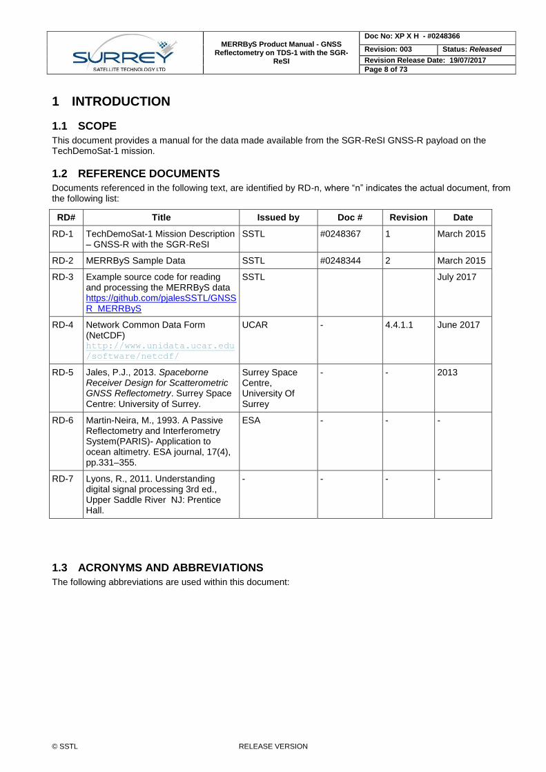
2 OVERVIEW
This document describes the data flow, dependencies and resulting data types for the elements of the TDS-1 GNSS-Reflectometry Ground Processing Project, sponsored by ESA. The data is provided through the MERRByS web service, which allows access to the low-level data and the resulting wind and wave measurements. From the website a selection of samples is additionally provided, with practical description in RD-2. Example source code for reading and processing the MERRByS data is provided in RD-3.
2.1 GNSS-R
The GNSS-R technique works in a way that is similar to both existing altimeter and scatterometer radar satellites, but eliminates the need for dedicated transmitters through using the existing GNSS transmitters.
Figure 2-1 GNSS-R Geometry
The GNSS-R receiver is sensitive to surface roughness around each of the GNSS transmitter-to-receiver specular points. The surface roughness causes the reflections from each GNSS transmitter to spread over a glistening zone around the specular reflection point. The receiver recovers the signal power from around the glistening zone through correlation of a replica GNSS signal at a map of delay and Doppler offsets (DDM). These DDM images are then inverted back to a measurement of the surface roughness, such as that caused by wind driven waves. The receiver processes the direct signals for determining position, velocity and time and the reflected signals for remote sensing as in Figure 2-1. As the receiver moves, the specular point moves with it, starting off ahead of the receiver and slowly passing behind as the receiver moves under the higher, slower moving GNSS transmitter. The specular point traces out a path over the ocean surface which we call it’s “track”. The receiver can process multiple simultaneous tracks, from multiple GNSS-transmitters. GNSS reflections are not only off the ocean, but also off land, snow and ice, opening up other potential new opportunities for remote sensing – for example, measuring the thickness of sea ice, snow depth, soil moisture levels and the classification of vegetative foliage.
3 TECHDEMOSAT-1 GNSS-R EXPERIMENT
Investments in GNSS-R by the UK and the European Space Agency over the past few years are making it possible for Surrey Satellite Technology Ltd to launch a new GNSS-R payload onboard the TechDemoSat-1 (TDS-1; see Figure 3-1) satellite. This was launched in July 2014 carrying the GNSS-R payload as part of the Sea State Payload suite (SSP) that also includes a demonstration altimeter. Furthermore the same GNSS-R instrument has been selected to fly on the NASA EV-2 CYGNSS satellite constellation to measure hurricanes.
MERRByS Product Manual - GNSS Reflectometry on TDS-1 with the SGR-
ReSI
Doc No: XP X H - #0248366
Revision: 003 Status: Released
Revision Release Date: 19/07/2017
Page 11 of 73
© SSTL RELEASE VERSION
For a description of the TechDemoSat-1 mission and details of the GNSS-R receiver, the SGR-ReSI, see RD-1.
3.1 THE SGR-RESI
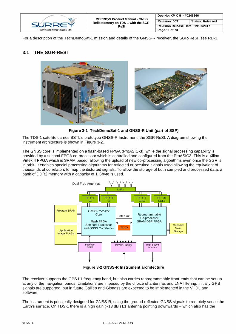
Figure 3-1 TechDemoSat-1 and GNSS-R Unit (part of SSP)
The TDS-1 satellite carries SSTL’s prototype GNSS-R Instrument, the SGR-ReSI. A diagram showing the instrument architecture is shown in Figure 3-2. The GNSS core is implemented on a flash-based FPGA (ProASIC-3), while the signal processing capability is provided by a second FPGA co-processor which is controlled and configured from the ProASIC3. This is a Xilinx Virtex 4 FPGA which is SRAM based, allowing the upload of new co-processing algorithms even once the SGR is in orbit. It enables special processing algorithms for reflected or occulted signals used allowing the equivalent of thousands of correlators to map the distorted signals. To allow the storage of both sampled and processed data, a bank of DDR2 memory with a capacity of 1 Gbyte is used.
GNSS Receiver Core
Flash FPGA
Soft core Processor and GNSS Correlators
Reprogrammable
Co-processor SRAM DSP FPGA
Program SRAM
Interface: SBPP
High Speed Interface
Application
Image FLASH
RF F/E L1/L2
RF F/E L1/L2
LNAs
RF F/E
L1
Power Supply
interlink
TCXO
Dual Freq Antennas
RF F/E L1
Onboard Mass
Storage
Figure 3-2 GNSS-R Instrument architecture
The receiver supports the GPS L1 frequency band, but also carries reprogrammable front-ends that can be set up at any of the navigation bands. Limitations are imposed by the choice of antennas and LNA filtering. Initially GPS signals are supported, but in future Galileo and Glonass are expected to be implemented in the VHDL and software. The instrument is principally designed for GNSS-R, using the ground-reflected GNSS signals to remotely sense the Earth’s surface. On TDS-1 there is a high gain (~13 dBi) L1 antenna pointing downwards – which also has the
MERRByS Product Manual - GNSS Reflectometry on TDS-1 with the SGR-
ReSI
Doc No: XP X H - #0248366
Revision: 003 Status: Released
Revision Release Date: 19/07/2017
Page 12 of 73
© SSTL RELEASE VERSION
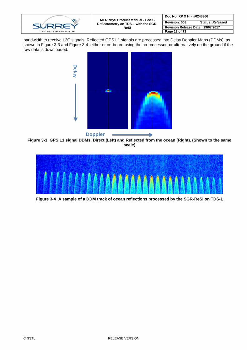
bandwidth to receive L2C signals. Reflected GPS L1 signals are processed into Delay Doppler Maps (DDMs), as shown in Figure 3-3 and Figure 3-4, either or on-board using the co-processor, or alternatively on the ground if the raw data is downloaded.
Figure 3-3 GPS L1 signal DDMs. Direct (Left) and Reflected from the ocean (Right). (Shown to the same scale)
Figure 3-4 A sample of a DDM track of ocean reflections processed by the SGR-ReSI on TDS-1
Doppler
Dela
y

MERRByS Product Manual - GNSS Reflectometry on TDS-1 with the SGR-
ReSI
Doc No: XP X H - #0248366
Revision: 003 Status: Released
Revision Release Date: 19/07/2017
Page 13 of 73
© SSTL RELEASE VERSION
4 DATA ACCESS POLICY
TDS-1 cannot offer a continuous GNSS-R data service due to foreseen early operational debugging & testing, validation and intermittent operation (it shares the satellite with 7 other payloads). Nevertheless MERRByS is intended to be a forerunner of a data service that may be offered by subsequent satellites, or constellations carrying the same payload. TDS-1 GNSS-R data sets are being released to allow users and researchers to experiment with the data, and investigate techniques for exploitation.
4.1 LICENCE
TDS-1 GNSS-R data is shared under Creative Commons Attribution Non-Commercial Data Licence (CC BY-NC), which can be supplemented by an additional licence permitting commercial exploitation if and when necessary.
CC
BY
NC
The Creative Commons (CC) Licence is designed for allowing the sharing of newly created data in a controlled way. The Creative Commons Attribution Non-Commercial Licence (CC BY-NC) ensures attribution, but also specifically restricts commercial use. The definition is “Non-Commercial means not primarily intended for or directed towards commercial advantage or monetary compensation” so allows some flexibility. By extending CC BY-NC into a CC+ licence, a commercial licence may later be awarded for specific users on top of the non-commercial licence, to allow licenced use for commercial purposes. The Creative Commons Attribution-NonCommercial 4.0 International License is available form http://creativecommons.org/licenses/by-nc/4.0/
4.2 DATA SETS
A set of sample data is available giving examples of L1 data over ocean, ice and land, L2 over ocean, and two L0 data sets over land and ocean. The full catalogue of L1 and L2 data requires application for a password from [email protected]. The application form requests information about the user, and their intended use for the GNSS-R data, and encourages feedback towards future improvements to the data service. Data is accessible via the MERRByS.org (or MERRByS.co.uk) website. Example source code for reading and processing the data are provided at https://github.com/pjalesSSTL/GNSSR_MERRByS
MERRByS Product Manual - GNSS Reflectometry on TDS-1 with the SGR-
ReSI
Doc No: XP X H - #0248366
Revision: 003 Status: Released
Revision Release Date: 19/07/2017
Page 14 of 73
© SSTL RELEASE VERSION
5 DATA OVERVIEW
5.1 PRODUCT DEFINITIONS
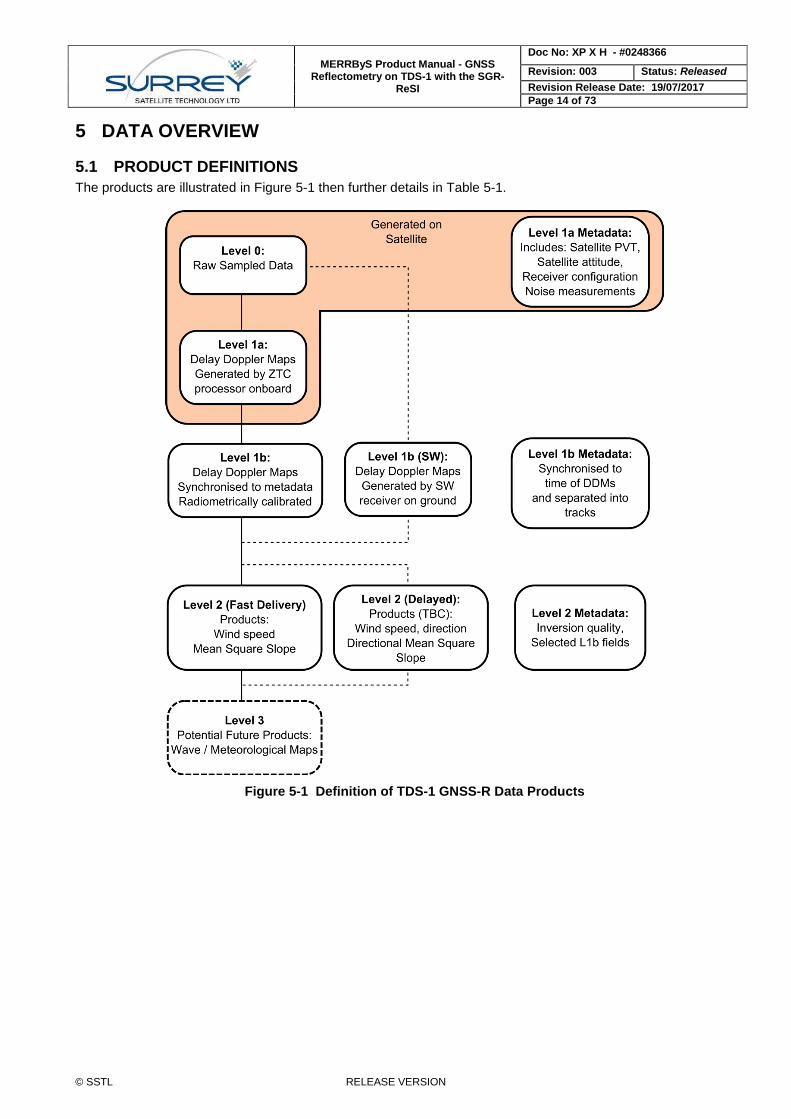
The products are illustrated in Figure 5-1 then further details in Table 5-1.
Figure 5-1 Definition of TDS-1 GNSS-R Data Products
MERRByS Product Manual - GNSS Reflectometry on TDS-1 with the SGR-
ReSI
Doc No: XP X H - #0248366
Revision: 003 Status: Released
Revision Release Date: 19/07/2017
Page 15 of 73
© SSTL RELEASE VERSION
Table 5-1 Data Product Description
Level / Description Data Metadata
Level 0 Raw Collections of digitised intermediate frequency samples
L0 Raw sampled data from both nadir and zenith antennas. Quantised to 2 bits with specified sample rate and intermediate frequency. Data stream contains all GNSS signals in the filter bandwidth visible to zenith and nadir antennas. Collection time of 1-4 minutes, depending on number of antenna inputs logged
Relevant SGR-ReSI packet data to geo-locate and timestamp the collection
Level 1 Reflections processed into DDMs
L1b(SW) Post processed from L0 to L1b(SW) through post-processing on the ground using a software receiver. Data length 1-4 minutes as per L0 data. Several processing levels are provided: to reproduce DDMs in similar approach to onboard and to produce higher-resolution DDMs.
Extracted metadata from processing the L0 data samples and from the receiver’s real-time SBPP format.
L1a Real time onboard processing into DDMs using the SGR-ReSI’s ZTC processing unit. Typically near to 24 hrs of data per day (within operational constraints). Simultaneous processing of 4 reflection channels. Tracks are interleaved in High Speed Interface files with L0 raw collections. L0 data corresponding to the L1a/b data is not generally available as L1a is directly processed onboard.
SGR-ReSI SBPP format position velocity and time information at low rate and unsynchronised to the time of the DDMs. Platform state including satellite attitude
L1b Data converted from the L1a onboard processed DDMs and converted to NetCDF format. The DDMs are separated into tracks and referenced to files with synchronised metadata. Typically near to 24 hrs of data per day (within operational constraints).
Metadata extracted from the receiver SBPP and the DDMs. Metadata is synchronised to the time of each DDM. Contains metadata common to all tracks (e.g. receiver position) and track-specific metadata for each DDM. Metadata from the lower rate receiver SBPP format is interpolated to match the time of the DDMs.
Level 2 Derived geophysical parameters
L2(FDI) Fast Delivery: Mean square slope, wind speed Processed from L1b
L1b and L2 metadata, including quality figure
L2(DM) Delayed Mode: A potential future data product generated from fitting of DDMs may allow recovery of directional information about wind and
L1 and L2 metadata, including quality figure
MERRByS Product Manual - GNSS Reflectometry on TDS-1 with the SGR-
ReSI
Doc No: XP X H - #0248366
Revision: 003 Status: Released
Revision Release Date: 19/07/2017
Page 16 of 73
© SSTL RELEASE VERSION
waves. Processed from L1b or L1b(SW)
The L0, L1b, and L2(FDI) output products are made available through the MERRByS catalogue and web service under the CC-BY-NC license from Section 4.
5.1.1 Differences of TDS-1 from CYGNSS Products
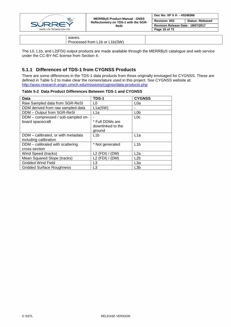
There are some differences in the TDS-1 data products from those originally envisaged for CYGNSS. These are defined in Table 5-2 to make clear the nomenclature used in this project. See CYGNSS website at: http://aoss-research.engin.umich.edu/missions/cygnss/data-products.php
Table 5-2 Data Product Differences Between TDS-1 and CYGNSS
Data TDS-1 CYGNSS
Raw Sampled data from SGR-ReSI L0 L0a
DDM derived from raw sampled data L1a(SW) -
DDM – Output from SGR-ReSI L1a L0b
DDM – compressed / sub-sampled on-board spacecraft
- * Full DDMs are downlinked to the ground
L0c
DDM – calibrated, or with metadata including calibration
L1b L1a
DDM – calibrated with scattering cross-section
* Not generated L1b
Wind Speed (tracks) L2 (FDI) / (DM) L2a
Mean Squared Slope (tracks) L2 (FDI) / (DM) L2b
Gridded Wind Field L3 L3a
Gridded Surface Roughness L3 L3b
MERRByS Product Manual - GNSS Reflectometry on TDS-1 with the SGR-
ReSI
Doc No: XP X H - #0248366
Revision: 003 Status: Released
Revision Release Date: 19/07/2017
Page 17 of 73
© SSTL RELEASE VERSION
6 L0 – RAW COLLECTIONS
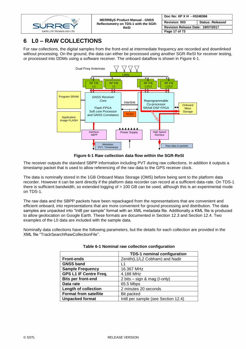
For raw collections, the digital samples from the front-end at intermediate frequency are recorded and downlinked without processing. On the ground, the data can either be processed using another SGR-ReSI for receiver testing, or processed into DDMs using a software receiver. The onboard dataflow is shown in Figure 6-1.
GNSS Receiver Core
Flash FPGA
Soft core Processor and GNSS Correlators
Reprogrammable
Co-processor SRAM DSP FPGA
Program SRAM
Application
Image FLASH
RF F/E L1/L2
RF F/E L1/L2
LNAs
RF F/E
L1
Power Supply
interlink
TCXO
Dual Freq Antennas
RF F/E L1
Onboard Mass
Storage
High Speed Interface
Interface: SBPP
Metadata: PVT, Timestamps
Raw data in packets
Figure 6-1 Raw collection data flow within the SGR-ReSI
The receiver outputs the standard SBPP information including PVT during raw collections. In addition it outputs a timestamp packet that is used to allow referencing of the raw data to the GPS receiver clock. The data is nominally stored in the 1GB Onboard Mass Storage (OMS) before being sent to the platform data recorder. However it can be sent directly if the platform data recorder can record at a sufficient data-rate. On TDS-1 there is sufficient bandwidth, so extended logging of > 100 GB can be used, although this is an experimental mode on TDS-1. The raw data and the SBPP packets have been repackaged from the representations that are convenient and efficient onboard, into representations that are more convenient for ground processing and distribution. The data samples are unpacked into “Int8 per sample” format with an XML metadata file. Additionally a KML file is produced to allow geolocation on Google Earth. These formats are documented in Section 12.3 and Section 12.4. Two examples of the L0 data are included with the sample data. Nominally data collections have the following parameters, but the details for each collection are provided in the XML file “TrackSearchRawCollectionFile”.
Table 6-1 Nominal raw collection configuration
TDS-1 nominal configuration
Front-ends Zenith(L1/L2 Cobham) and Nadir
GNSS band L1
Sample Frequency 16.367 MHz
GPS L1 IF Centre Freq. 4.188 MHz
Bits per front-end 2 bits – sign & mag (I-only)
Data rate 65.5 Mbps
Length of collection 2 minutes 20 seconds
Format from satellite Bit packed
Unpacked format Int8 per sample (see Section 12.4)
MERRByS Product Manual - GNSS Reflectometry on TDS-1 with the SGR-
ReSI
Doc No: XP X H - #0248366
Revision: 003 Status: Released
Revision Release Date: 19/07/2017
Page 18 of 73
© SSTL RELEASE VERSION
7 L1A - ONBOARD PROCESSING
7.1 SGR-RESI PROCESSING FUNCTIONS
The SGR-ReSI reflectometry onboard processing flow is shown in Figure 7-1. This section gives an overview of the onboard algorithms, focusing on the details relevant to the processing of the down-stream products.
Data Samples from Zenith
Antenna
Data Samples from Nadir Antenna
Navigation Correlators
(Flash FPGA)
Signal acquisition, track, decode, pseudorange construction
Determine Specular
Reflection Points
Si
Determine GNSS transmit positions from Ephemeris
Ti
Determine accurate time and Receiver position
R
Process Data stream into Delay
Doppler Map (Co-processor)
Calculate Delay Doppler (DD) estimates for
TSRi
Output as SBPP Position, Velocity,
Time, Reflectometry
metadata
Zenith Antenna
Nadir Antenna
Sampled Nadir Data Output over HSI DDMs
Figure 7-1 Schematic representation of the GNSS-R DDM processing flow. Bold boxes indicate focus of this section
7.1.1 Reflection Tracking
Reflected GNSS signals are weak and distorted, and so standard GNSS closed loop tracking techniques are not possible. Instead a geometrically-derived estimate of delay and Doppler can be calculated for each reflection within the satellite’s footprint in order to prime the Digitally Controlled Oscillators (DCOs) of the DDM co-processor. Three specific algorithms are required: a) Specular point location calculation, b) Calculation of the delay and Doppler estimates for the specular reflection path. c) Allocation of reflections to processing channels.
7.1.1.1 Specular Point Location
The specular point is the location on the Earth’s surface, by the laws of reflection, where the incident and reflection rays have equal angle to the surface normal. Alternatively the definition is the point on the Earth which has the minimum path-length from transmitter to Earth to receiver. To determine the specular point location a model for the Earth’s surface is needed. There are a number of approaches with different Earth models: from the spherical Earth approximation, to ellipsoidal earth or using a digital elevation model. The SGR-ReSI system relies on real-time geometrical tracking to centre the DDM on the reflection. This makes the computational time and accuracy of the Earth model part of the trade-off space in the receiver design. A method is needed that can be processed on-board which meets the accuracy requirements for tracking the reflections within the DDM window. A method identified as having a good balance is the quasi-spherical Earth method. This is proposed in [RD-5 Jales 2013] and is shown again here in section 13.1.
7.1.1.2 Delay and Doppler Determination
For real-time processing the DDM correlators need to be steered to the location of the specular point. This requires the internal replica code delay and carrier frequency (of the chosen offset in the DDM) to match that of the reflection signal. The expected delay and Doppler is calculated given the position and velocities of the transmitter and receiver and the specular point location.
MERRByS Product Manual - GNSS Reflectometry on TDS-1 with the SGR-
ReSI
Doc No: XP X H - #0248366
Revision: 003 Status: Released
Revision Release Date: 19/07/2017
Page 19 of 73
© SSTL RELEASE VERSION
The open-loop reflection tracking scheme runs in the SGR-ReSI receiver in real-time. The implementation of the tracking is specifically designed to provide the tracking updates to the DDM processor synchronised to the direct signals despite the calculation latency. To do this the receiver, transmitter and specular point locations are updated at a rate of 1 Hz, used to calculate the tracking parameters, which are then extrapolated to provide 10 Hz updates. The updates are applied to each reflection channel’s code phase, code rate and carrier frequency.
7.1.1.3 Allocation
The aim of the allocation algorithm is to choose the reflections to track that have the highest signal to noise ratio. This is based on the assumption that a higher signal to noise ratio in the DDM will result in a better estimation of the scattering cross-section of the surface. For the chosen allocation algorithm, the difference in signal to noise ratio between the available reflections is assumed to be dominated by the antenna gain pointed at each. The reflection channel allocation approach creates a sorted list of reflections, with the ‘best’ reflections (those with the highest antenna gain) at the top of the list. The allocation algorithm then uses this list to allocate the top four reflections to the four reflectometry channels, taking into account which of the antennas has the highest gain towards the reflection. The algorithm can work for multiple nadir antennas, the TDS-1 receiver uses one antenna and the CYGNSS receiver uses two. Inputs to the algorithm are the list of vectors from receiver to each of the specular points, the antenna boresight vector, antenna gain pattern and satellite attitude. See Section 13.2 for further definitions.
7.1.2 DDM Processing (The ZTC)
The DDM processing is performed in the reconfigurable co-processor and follows the work implemented in [RD-5 Jales 2013]. The processing approach calculates the Doppler pixels in the frequency domain to reduce the computational complexity. This approach was chosen due to its suitability for implementation in an FPGA. The implementation of this approach is called the Zoom Transform Correlator (ZTC). The diagrammatic representation of this technique is shown in Figure 7-2. The advantage of this approach over that of individual discrete correlators per pixel is that the computational complexity can be reduced as the frequency search reduces to spectrum estimation, for which there are techniques that scale considerably better than with the number of pixels. Each reflection channel is composed of the processing steps in Figure 7-2. Firstly a coarse carrier ‘wipe-off’ is performed to down-convert such that 0 Hz is the centre of the DDM, corresponding to the carrier frequency (including Doppler shift) of the specular path. This is followed by a set of channels that ‘wipe-off’ the code, each configured for the delay of a separate DDM row. The result of the coarse carrier wipe-off and code wipe-off leaves a demodulated signal at a small residual range of Doppler frequencies. This contains the full spectrum of Doppler shifts present for the chosen code phase. Performing spectrum estimation on it will return one row of DDM pixels simultaneously.
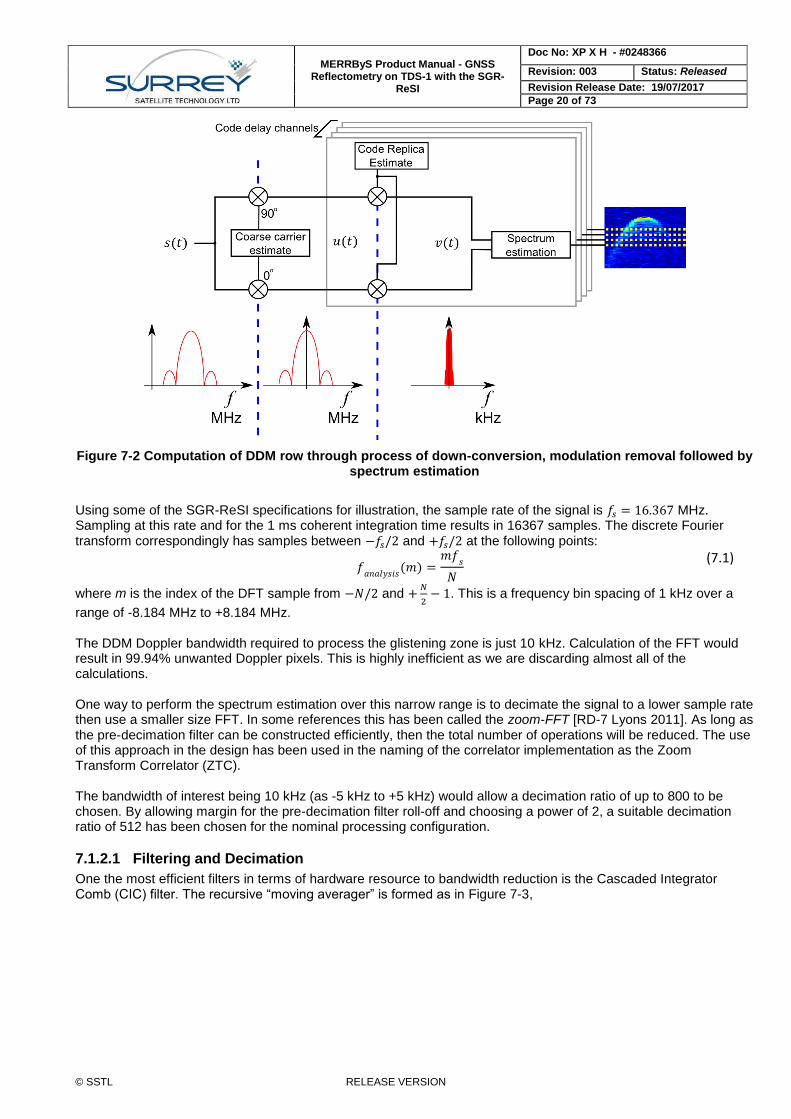
MERRByS Product Manual - GNSS Reflectometry on TDS-1 with the SGR-
ReSI
Doc No: XP X H - #0248366
Revision: 003 Status: Released
Revision Release Date: 19/07/2017
Page 20 of 73
© SSTL RELEASE VERSION
Figure 7-2 Computation of DDM row through process of down-conversion, modulation removal followed by spectrum estimation
Using some of the SGR-ReSI specifications for illustration, the sample rate of the signal is 𝑓𝑠 = 16.367 MHz. Sampling at this rate and for the 1 ms coherent integration time results in 16367 samples. The discrete Fourier transform correspondingly has samples between −𝑓𝑠/2 and +𝑓𝑠/2 at the following points:
𝑓
𝑎𝑛𝑎𝑙𝑦𝑠𝑖𝑠(𝑚) =
𝑚𝑓𝑠
𝑁
(7.1)
where m is the index of the DFT sample from −𝑁/2 and +𝑁
2− 1. This is a frequency bin spacing of 1 kHz over a
range of -8.184 MHz to +8.184 MHz. The DDM Doppler bandwidth required to process the glistening zone is just 10 kHz. Calculation of the FFT would result in 99.94% unwanted Doppler pixels. This is highly inefficient as we are discarding almost all of the calculations. One way to perform the spectrum estimation over this narrow range is to decimate the signal to a lower sample rate then use a smaller size FFT. In some references this has been called the zoom-FFT [RD-7 Lyons 2011]. As long as the pre-decimation filter can be constructed efficiently, then the total number of operations will be reduced. The use of this approach in the design has been used in the naming of the correlator implementation as the Zoom Transform Correlator (ZTC). The bandwidth of interest being 10 kHz (as -5 kHz to +5 kHz) would allow a decimation ratio of up to 800 to be chosen. By allowing margin for the pre-decimation filter roll-off and choosing a power of 2, a suitable decimation ratio of 512 has been chosen for the nominal processing configuration.
7.1.2.1 Filtering and Decimation
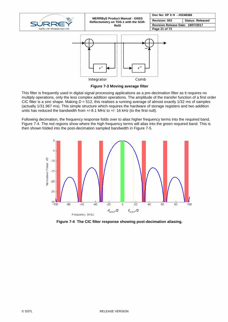
One the most efficient filters in terms of hardware resource to bandwidth reduction is the Cascaded Integrator Comb (CIC) filter. The recursive “moving averager” is formed as in Figure 7-3,
MERRByS Product Manual - GNSS Reflectometry on TDS-1 with the SGR-
ReSI
Doc No: XP X H - #0248366
Revision: 003 Status: Released
Revision Release Date: 19/07/2017
Page 21 of 73
© SSTL RELEASE VERSION
Figure 7-3 Moving average filter
This filter is frequently used in digital signal processing applications as a pre-decimation filter as it requires no multiply operations, only the less complex addition operations. The amplitude of the transfer function of a first order CIC filter is a sinc shape. Making D = 512, this realises a running average of almost exactly 1/32 ms of samples (actually 1/31.967 ms). This simple structure which requires the hardware of storage registers and two addition units has reduced the bandwidth from +/-8.1 MHz to +/- 16 kHz (to the first null). Following decimation, the frequency response folds over to alias higher frequency terms into the required band, Figure 7-4. The red regions show where the high frequency terms will alias into the green required band. This is then shown folded into the post-decimation sampled bandwidth in Figure 7-5.
Figure 7-4 The CIC filter response showing post-decimation aliasing.
MERRByS Product Manual - GNSS Reflectometry on TDS-1 with the SGR-
ReSI
Doc No: XP X H - #0248366
Revision: 003 Status: Released
Revision Release Date: 19/07/2017
Page 22 of 73
© SSTL RELEASE VERSION
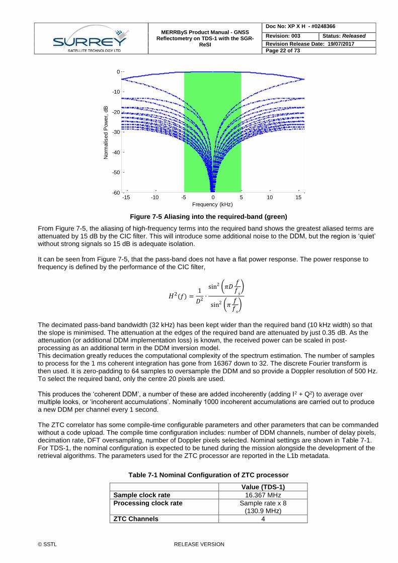
Figure 7-5 Aliasing into the required-band (green)
From Figure 7-5, the aliasing of high-frequency terms into the required band shows the greatest aliased terms are attenuated by 15 dB by the CIC filter. This will introduce some additional noise to the DDM, but the region is ‘quiet’ without strong signals so 15 dB is adequate isolation. It can be seen from Figure 7-5, that the pass-band does not have a flat power response. The power response to frequency is defined by the performance of the CIC filter,
𝐻2(𝑓) =1
𝐷2 ∙
sin2 (𝜋𝐷𝑓𝑓
𝑠
)
sin2 (𝜋𝑓𝑓
𝑠
)
The decimated pass-band bandwidth (32 kHz) has been kept wider than the required band (10 kHz width) so that the slope is minimised. The attenuation at the edges of the required band are attenuated by just 0.35 dB. As the attenuation (or additional DDM implementation loss) is known, the received power can be scaled in post-processing as an additional term in the DDM inversion model. This decimation greatly reduces the computational complexity of the spectrum estimation. The number of samples to process for the 1 ms coherent integration has gone from 16367 down to 32. The discrete Fourier transform is then used. It is zero-padding to 64 samples to oversample the DDM and so provide a Doppler resolution of 500 Hz. To select the required band, only the centre 20 pixels are used. This produces the ‘coherent DDM’, a number of these are added incoherently (adding I2 + Q2) to average over multiple looks, or ‘incoherent accumulations’. Nominally 1000 incoherent accumulations are carried out to produce a new DDM per channel every 1 second. The ZTC correlator has some compile-time configurable parameters and other parameters that can be commanded without a code upload. The compile time configuration includes: number of DDM channels, number of delay pixels, decimation rate, DFT oversampling, number of Doppler pixels selected. Nominal settings are shown in Table 7-1. For TDS-1, the nominal configuration is expected to be tuned during the mission alongside the development of the retrieval algorithms. The parameters used for the ZTC processor are reported in the L1b metadata.
Table 7-1 Nominal Configuration of ZTC processor
Value (TDS-1)
Sample clock rate 16.367 MHz
Processing clock rate Sample rate x 8 (130.9 MHz)
ZTC Channels 4
-15 -10 -5 0 5 10 15-60
-50
-40
-30
-20
-10
0
Frequency (kHz)
Norm
alis
ed P
ow
er,
dB
MERRByS Product Manual - GNSS Reflectometry on TDS-1 with the SGR-
ReSI
Doc No: XP X H - #0248366
Revision: 003 Status: Released
Revision Release Date: 19/07/2017
Page 23 of 73
© SSTL RELEASE VERSION
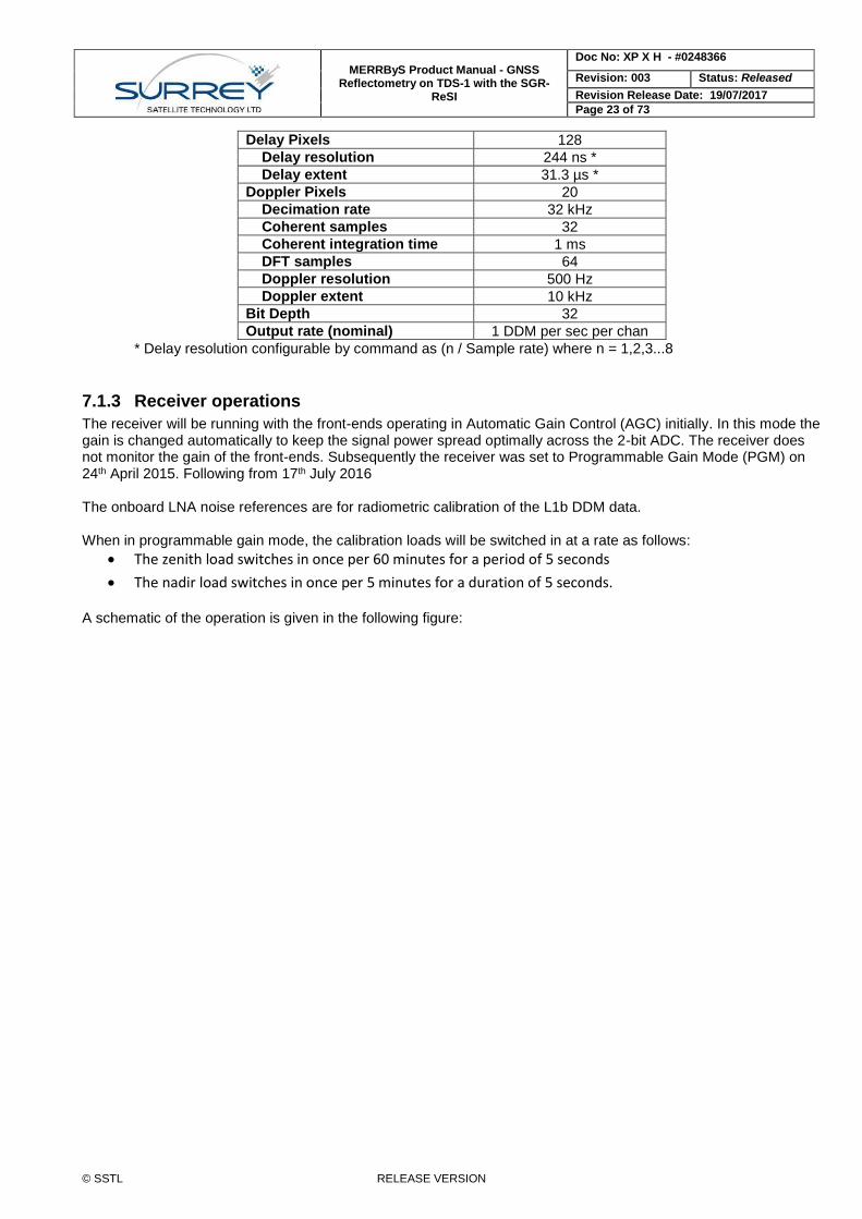
Delay Pixels 128
Delay resolution 244 ns *
Delay extent 31.3 µs *
Doppler Pixels 20
Decimation rate 32 kHz
Coherent samples 32
Coherent integration time 1 ms
DFT samples 64
Doppler resolution 500 Hz
Doppler extent 10 kHz
Bit Depth 32
Output rate (nominal) 1 DDM per sec per chan
* Delay resolution configurable by command as (n / Sample rate) where n = 1,2,3...8
7.1.3 Receiver operations
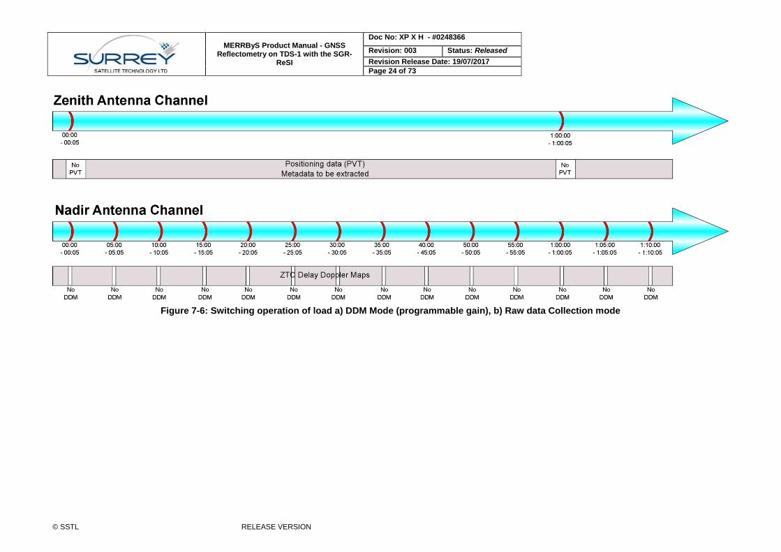
The receiver will be running with the front-ends operating in Automatic Gain Control (AGC) initially. In this mode the gain is changed automatically to keep the signal power spread optimally across the 2-bit ADC. The receiver does not monitor the gain of the front-ends. Subsequently the receiver was set to Programmable Gain Mode (PGM) on 24th April 2015. Following from 17th July 2016 The onboard LNA noise references are for radiometric calibration of the L1b DDM data. When in programmable gain mode, the calibration loads will be switched in at a rate as follows:
The zenith load switches in once per 60 minutes for a period of 5 seconds
The nadir load switches in once per 5 minutes for a duration of 5 seconds.
A schematic of the operation is given in the following figure:
MERRByS Product Manual - GNSS Reflectometry on TDS-1 with the SGR-
ReSI
Doc No: XP X H - #0248366
Revision: 003 Status: Released
Revision Release Date: 19/07/2017
Page 24 of 73
© SSTL RELEASE VERSION
Figure 7-6: Switching operation of load a) DDM Mode (programmable gain), b) Raw data Collection mode
MERRByS Product Manual - GNSS Reflectometry on TDS-1 with the SGR-
ReSI
Doc No: XP X H - #0248366
Revision: 003 Status: Released
Revision Release Date: 19/07/2017
Page 25 of 73
© SSTL RELEASE VERSION
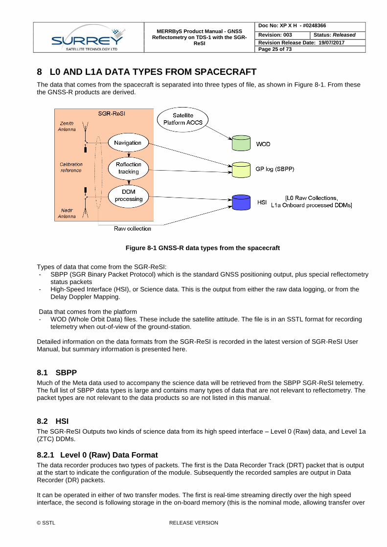
8 L0 AND L1A DATA TYPES FROM SPACECRAFT
The data that comes from the spacecraft is separated into three types of file, as shown in Figure 8-1. From these the GNSS-R products are derived.
Figure 8-1 GNSS-R data types from the spacecraft
Types of data that come from the SGR-ReSI: - SBPP (SGR Binary Packet Protocol) which is the standard GNSS positioning output, plus special reflectometry
status packets - High-Speed Interface (HSI), or Science data. This is the output from either the raw data logging, or from the
Delay Doppler Mapping. Data that comes from the platform - WOD (Whole Orbit Data) files. These include the satellite attitude. The file is in an SSTL format for recording
telemetry when out-of-view of the ground-station. Detailed information on the data formats from the SGR-ReSI is recorded in the latest version of SGR-ReSI User Manual, but summary information is presented here.
8.1 SBPP
Much of the Meta data used to accompany the science data will be retrieved from the SBPP SGR-ReSI telemetry. The full list of SBPP data types is large and contains many types of data that are not relevant to reflectometry. The packet types are not relevant to the data products so are not listed in this manual.
8.2 HSI
The SGR-ReSI Outputs two kinds of science data from its high speed interface – Level 0 (Raw) data, and Level 1a (ZTC) DDMs.
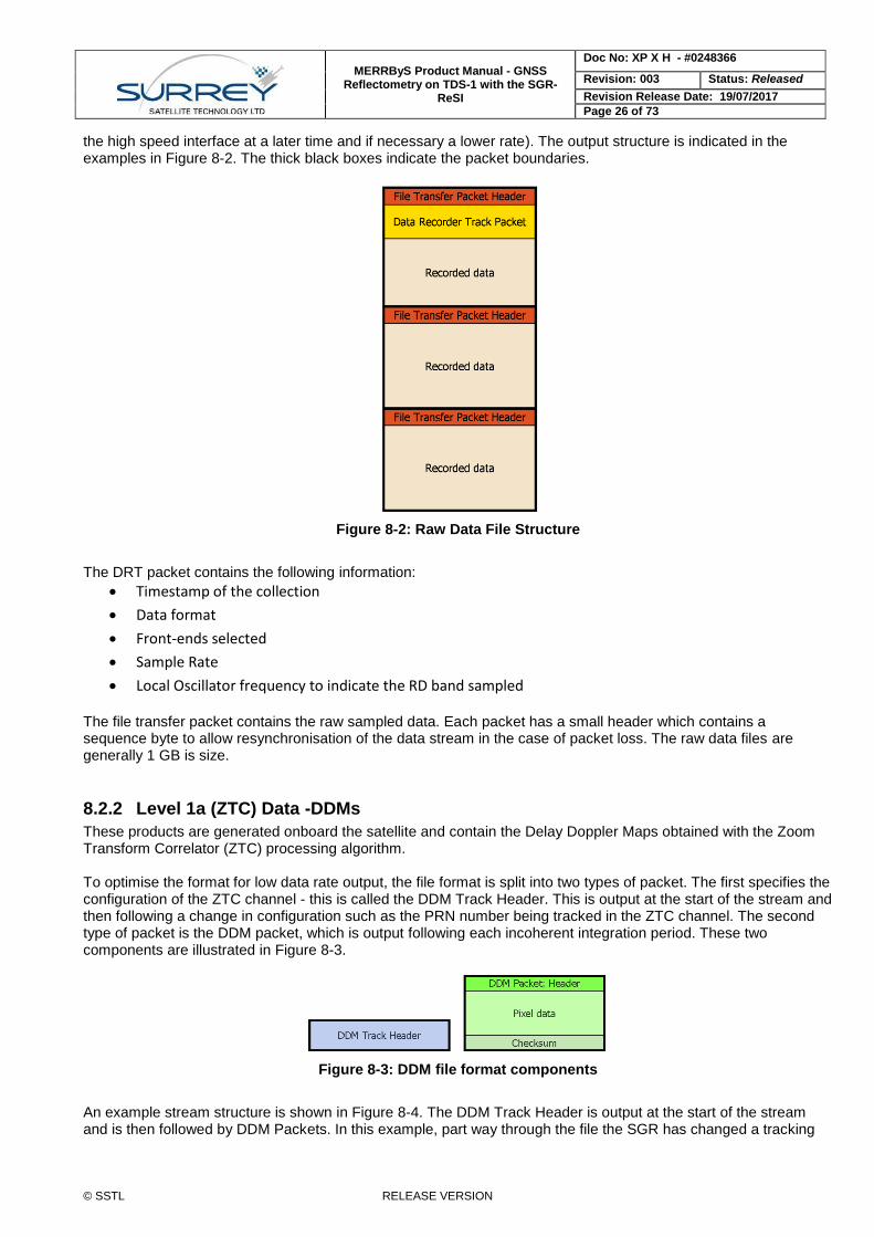
8.2.1 Level 0 (Raw) Data Format
The data recorder produces two types of packets. The first is the Data Recorder Track (DRT) packet that is output at the start to indicate the configuration of the module. Subsequently the recorded samples are output in Data Recorder (DR) packets. It can be operated in either of two transfer modes. The first is real-time streaming directly over the high speed interface, the second is following storage in the on-board memory (this is the nominal mode, allowing transfer over
MERRByS Product Manual - GNSS Reflectometry on TDS-1 with the SGR-
ReSI
Doc No: XP X H - #0248366
Revision: 003 Status: Released
Revision Release Date: 19/07/2017
Page 26 of 73
© SSTL RELEASE VERSION
the high speed interface at a later time and if necessary a lower rate). The output structure is indicated in the examples in Figure 8-2. The thick black boxes indicate the packet boundaries.
Figure 8-2: Raw Data File Structure
The DRT packet contains the following information:
Timestamp of the collection
Data format
Front-ends selected
Sample Rate
Local Oscillator frequency to indicate the RD band sampled
The file transfer packet contains the raw sampled data. Each packet has a small header which contains a sequence byte to allow resynchronisation of the data stream in the case of packet loss. The raw data files are generally 1 GB is size.
8.2.2 Level 1a (ZTC) Data -DDMs
These products are generated onboard the satellite and contain the Delay Doppler Maps obtained with the Zoom Transform Correlator (ZTC) processing algorithm. To optimise the format for low data rate output, the file format is split into two types of packet. The first specifies the configuration of the ZTC channel - this is called the DDM Track Header. This is output at the start of the stream and then following a change in configuration such as the PRN number being tracked in the ZTC channel. The second type of packet is the DDM packet, which is output following each incoherent integration period. These two components are illustrated in Figure 8-3.
Figure 8-3: DDM file format components
An example stream structure is shown in Figure 8-4. The DDM Track Header is output at the start of the stream and is then followed by DDM Packets. In this example, part way through the file the SGR has changed a tracking
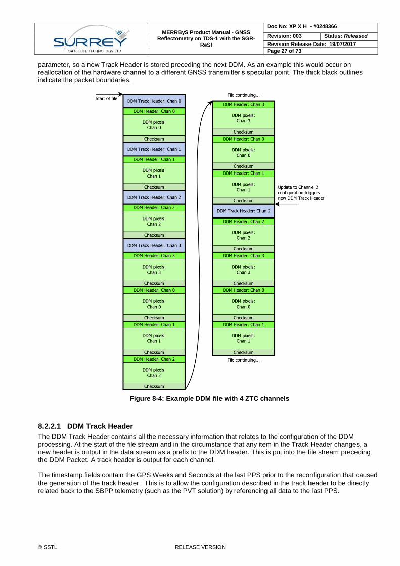
MERRByS Product Manual - GNSS Reflectometry on TDS-1 with the SGR-
ReSI
Doc No: XP X H - #0248366
Revision: 003 Status: Released
Revision Release Date: 19/07/2017
Page 27 of 73
© SSTL RELEASE VERSION
parameter, so a new Track Header is stored preceding the next DDM. As an example this would occur on reallocation of the hardware channel to a different GNSS transmitter’s specular point. The thick black outlines indicate the packet boundaries.
Figure 8-4: Example DDM file with 4 ZTC channels
8.2.2.1 DDM Track Header
The DDM Track Header contains all the necessary information that relates to the configuration of the DDM processing. At the start of the file stream and in the circumstance that any item in the Track Header changes, a new header is output in the data stream as a prefix to the DDM header. This is put into the file stream preceding the DDM Packet. A track header is output for each channel. The timestamp fields contain the GPS Weeks and Seconds at the last PPS prior to the reconfiguration that caused the generation of the track header. This is to allow the configuration described in the track header to be directly related back to the SBPP telemetry (such as the PVT solution) by referencing all data to the last PPS.
MERRByS Product Manual - GNSS Reflectometry on TDS-1 with the SGR-
ReSI
Doc No: XP X H - #0248366
Revision: 003 Status: Released
Revision Release Date: 19/07/2017
Page 28 of 73
© SSTL RELEASE VERSION
8.2.2.2 DDM Packet
The DDM Packet contains the DDM pixel data with a compact header to relate it to the configuration provided in the DDM Track Header. The pixel data is output at 32 bits per pixel.
9 L0 TO L1B(SW) GROUND PROCESSED DDMS
Format reference:
Inputs: L0 Raw data from TDS-1 (up to 4 minute file) containing at least data from 1 zenith and 1 nadir antenna.
Section 12.4
SBPP data from the receiver onboard navigation -
WOD data containing satellite attitude and orbit -
Outputs: L0 metadata describing the contents of the collection and geolocation
Section 12.3
L1b(SW) track of ground processed DDMs per satellite reflection
Section 12.6
L1b(SW) track metadata
L1b(SW) Receiver metadata file containing the receiver information common to all the tracks
Section 12.5
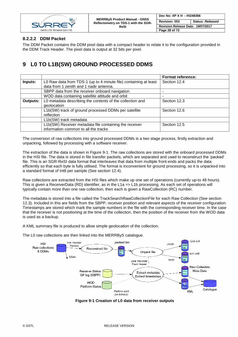
The conversion of raw collections into ground processed DDMs is a two stage process, firstly extraction and unpacking, followed by processing with a software receiver. The extraction of the data is shown in Figure 9-1. The raw collections are stored with the onboard processed DDMs in the HSI file. The data is stored in file transfer packets, which are separated and used to reconstruct the ‘packed’ file. This is an SGR-ReSI data format that interleaves that data from multiple front-ends and packs the data efficiently so that each byte is fully utilised. The format is inconvenient for ground processing, so it is unpacked into a standard format of Int8 per sample (See section 12.4). Raw collections are extracted from the HSI files which make up one set of operations (currently up-to 48 hours). This is given a ReceiverData (RD) identifier, as in the L1a => L1b processing. As each set of operations will typically contain more than one raw collection, then each is given a RawCollection (RC) number. The metadata is stored into a file called the TrackSearchRawCollectionFile for each Raw Collection (See section 12.3). Included in this are fields from the SBPP, receiver position and relevant aspects of the receiver configuration. Timestamps are stored which mark the sample numbers in the file with the corresponding receiver time. In the case that the receiver is not positioning at the time of the collection, then the position of the receiver from the WOD data is used as a backup. A KML summary file is produced to allow simple geolocation of the collection. The L0 raw collections are then linked into the MERRByS catalogue.
Figure 9-1 Creation of L0 data from receiver outputs
MERRByS Product Manual - GNSS Reflectometry on TDS-1 with the SGR-
ReSI
Doc No: XP X H - #0248366
Revision: 003 Status: Released
Revision Release Date: 19/07/2017
Page 29 of 73
© SSTL RELEASE VERSION
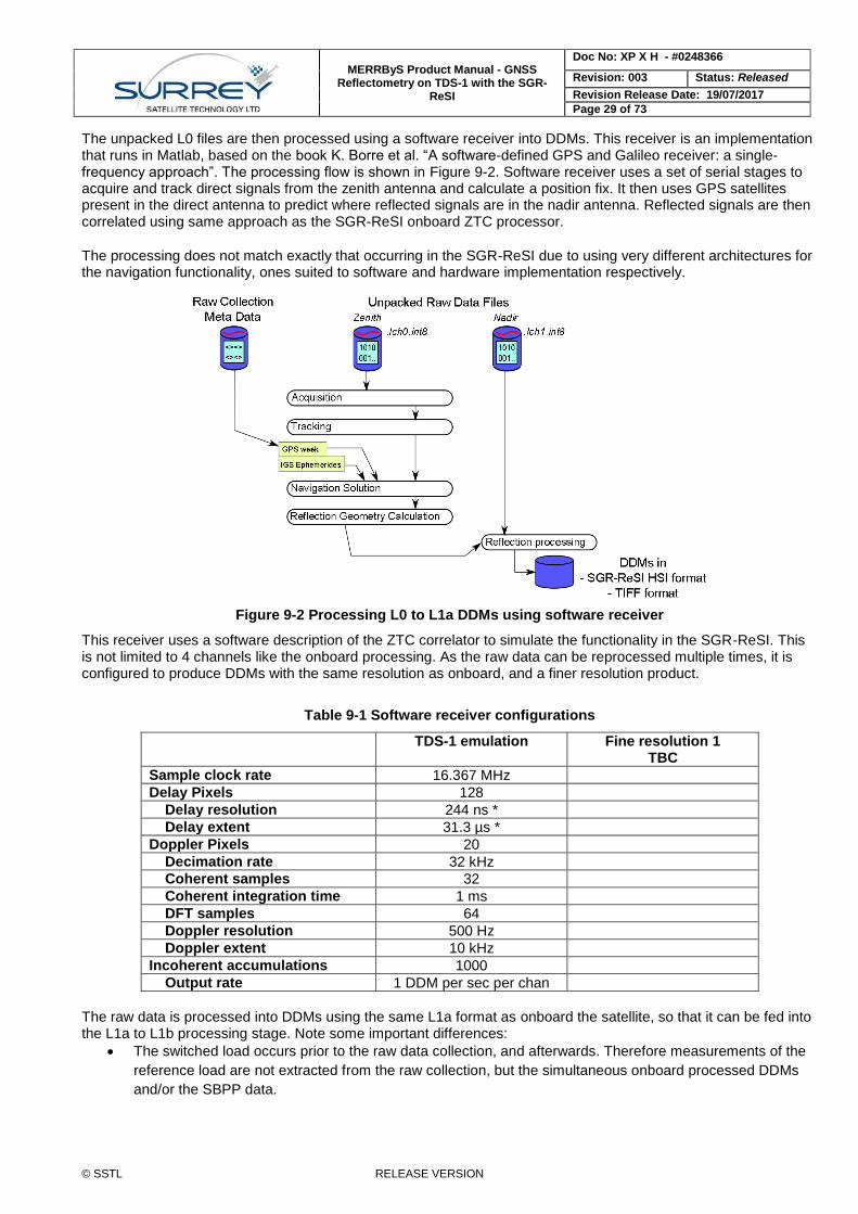
The unpacked L0 files are then processed using a software receiver into DDMs. This receiver is an implementation that runs in Matlab, based on the book K. Borre et al. “A software-defined GPS and Galileo receiver: a single-frequency approach”. The processing flow is shown in Figure 9-2. Software receiver uses a set of serial stages to acquire and track direct signals from the zenith antenna and calculate a position fix. It then uses GPS satellites present in the direct antenna to predict where reflected signals are in the nadir antenna. Reflected signals are then correlated using same approach as the SGR-ReSI onboard ZTC processor.
The processing does not match exactly that occurring in the SGR-ReSI due to using very different architectures for the navigation functionality, ones suited to software and hardware implementation respectively.
Figure 9-2 Processing L0 to L1a DDMs using software receiver
This receiver uses a software description of the ZTC correlator to simulate the functionality in the SGR-ReSI. This is not limited to 4 channels like the onboard processing. As the raw data can be reprocessed multiple times, it is configured to produce DDMs with the same resolution as onboard, and a finer resolution product.
Table 9-1 Software receiver configurations
TDS-1 emulation Fine resolution 1 TBC
Sample clock rate 16.367 MHz
Delay Pixels 128
Delay resolution 244 ns *
Delay extent 31.3 µs *
Doppler Pixels 20
Decimation rate 32 kHz
Coherent samples 32
Coherent integration time 1 ms
DFT samples 64
Doppler resolution 500 Hz
Doppler extent 10 kHz
Incoherent accumulations 1000
Output rate 1 DDM per sec per chan
The raw data is processed into DDMs using the same L1a format as onboard the satellite, so that it can be fed into the L1a to L1b processing stage. Note some important differences:
The switched load occurs prior to the raw data collection, and afterwards. Therefore measurements of the
reference load are not extracted from the raw collection, but the simultaneous onboard processed DDMs
and/or the SBPP data.
MERRByS Product Manual - GNSS Reflectometry on TDS-1 with the SGR-
ReSI
Doc No: XP X H - #0248366
Revision: 003 Status: Released
Revision Release Date: 19/07/2017
Page 30 of 73
© SSTL RELEASE VERSION
10 L1A TO L1B – DDM SYNCHRONISATION AND CALIBRATION
Format reference:
Inputs: L1a onboard processed DDMs -
L1a receiver status and PVT from SBPP file -
WOD data containing satellite attitude -
Antenna gain map for looking up the gain of the nadir antenna Section 12.7
Transmitter ephemeris giving the position of the transmitters -
Transmitter SVN to PRN mapping table -
Earth topographic map
Mission planning database
Outputs: L1b NetCDF Section 12.6
Catalogue outputs. Search tracks, quick look and summary images and KMZ file
-
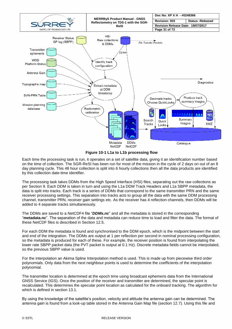
The processing flow takes the onboard processed DDMs and converts them into DDM products with synchronised metadata and radiometric calibration products. The overview of the data flow is shown in Figure 10-1 and described below. The detailed definitions are provided under the references above.
10.1 MERRBYS DATA SEGMENTATION
Data is split into 6 hour segments and given an identification string based on the centre of this collection period. The format consists of year, month, day and hour, 'yyyy-mm/dd/Hhh'. The time of collection is 3 hours prior and 3 hours after this data identifier.
Table 10-1 Data segmentation times
Data designation yyyy-MM/dd/Hhh Examples:
Start time Up-to (excluding)
2017-06/30/H00 21:00 03:00
2017-06/30/H06 03:00 09:00
2017-06/30/H12 09:00 15:00
2017-06/30/H18 15:00 21:00
MERRByS Product Manual - GNSS Reflectometry on TDS-1 with the SGR-
ReSI
Doc No: XP X H - #0248366
Revision: 003 Status: Released
Revision Release Date: 19/07/2017
Page 31 of 73
© SSTL RELEASE VERSION
Figure 10-1 L1a to L1b processing flow
Each time the processing task is run, it operates on a set of satellite data, giving it an identification number based on the time of collection. The SGR-ReSI has been run for most of the mission in the cycle of 2 days on out of an 8 day planning cycle. This 48 hour collection is split into 6 hourly collections then all the data products are identified by this collection date-time identifier. The processing task takes DDMs from the High Speed Interface (HSI) files, separating out the raw collections as per Section 9. Each DDM is taken in turn and using the L1a DDM Track Headers and L1a SBPP metadata, the data is split into tracks. Each track is a series of DDMs that correspond to the same transmitter PRN and the same receiver processing settings. This separation into tracks acts to group all the data with the same DDM processing channel, transmitter PRN, receiver gain settings etc. As the receiver has 4 reflection channels, then DDMs will be added to 4 separate tracks simultaneously. The DDMs are saved to a NetCDF4 file “DDMs.nc” and all the metadata is stored in the corresponding “metadata.nc”. The separation of the data and metadata can reduce time to load and filter the data. The format of these NetCDF files is described in Section 12.5. For each DDM the metadata is found and synchronised to the DDM epoch, which is the midpoint between the start and end of the integration. The DDMs are output at 1 per reflection per second in nominal processing configuration, so the metadata is produced for each of these. For example, the receiver position is found from interpolating the lower rate SBPP packet data (the PVT packet is output at 0.1 Hz). Discrete metadata fields cannot be interpolated, so the previous SBPP value is used. For the interpolation an Akima Spline Interpolation method is used. This is made up from piecewise third order polynomials. Only data from the next neighbour points is used to determine the coefficients of the interpolation polynomial. The transmitter location is determined at the epoch time using broadcast ephemeris data from the International GNSS Service (IGS). Once the position of the receiver and transmitter are determined, the specular point is recalculated. This determines the specular point location as calculated for the onboard tracking. The algorithm for which is defined in section 13.1. By using the knowledge of the satellite’s position, velocity and attitude the antenna gain can be determined. The antenna gain is found from a look-up table stored in the Antenna Gain Map file (section 12.7). Using this file and

MERRByS Product Manual - GNSS Reflectometry on TDS-1 with the SGR-
ReSI
Doc No: XP X H - #0248366
Revision: 003 Status: Released
Revision Release Date: 19/07/2017
Page 32 of 73
© SSTL RELEASE VERSION
the provided metadata one can calculate the antenna gain away from the specular ray. Only the receiver antenna gain pointed towards the specular point is provided in the metadata. A DDM is discarded from the dataset if any of a number of self-consistency checks fail (between SBPP and HSI packets). This discards DDMs from L1b for a number of reasons, including no coincident metadata available in the SBPP file and gaps in the data downloaded from the spacecraft. Many other fields are added to the metadata, as defined in sections 12.5. Radiometric Calibration The L1b data set DDMs are in units of ‘DDM Power Counts’. This is a power scale used in the receiver, subject to analogue and digital scaling. The metadata provided allows for the conversion of the DDM pixels to units of received power in Watts. This process is carried out using internal and external references according to the method detailed in Section 14.
10.2 CATALOGUE
The process creates a set of files to add to the MERRByS web catalogue. This is a set of “SearchTracks”, selected DDM images and Keyhole Mark-up language - Zipped (KMZ) files. The search tracks are a decimated version of the full track files. The decimation reduces the computational effort required for the catalogue server to search for tracks matching the search requests. The decimation is carried out such that the first, last and highest antenna gain DDMs are stored, then ones selected every 60 seconds. The single DDM, the ‘QuickLook’ is stored to Portable Network Graphics (PNG) format. This DDM is chosen to be the one with the time in the track when the highest antenna gain is pointed towards the specular point. A summary image is formed for display on the MERRByS catalogue server. The summary is a selection of up-to 30 DDMs selected, evenly spaced through the track to give an indication of the contents. The KMZ file contains a summary of the data viewable in Google Earth. The retrievals are stored in the file for display using “Right Click>Show Elevation Data”. Further details are given for the sample data RD-2.
MERRByS Product Manual - GNSS Reflectometry on TDS-1 with the SGR-
ReSI
Doc No: XP X H - #0248366
Revision: 003 Status: Released
Revision Release Date: 19/07/2017
Page 33 of 73
© SSTL RELEASE VERSION
11 L1B TO L2 – GEOPHYSICAL RETRIEVAL
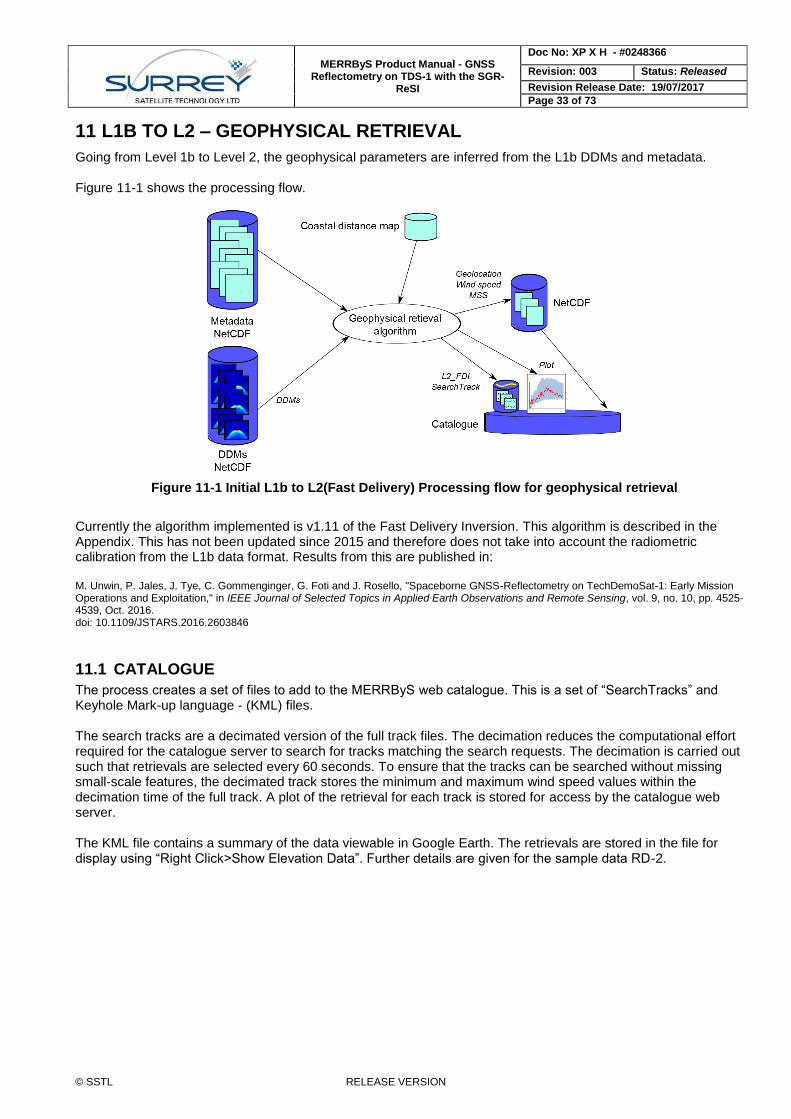
Going from Level 1b to Level 2, the geophysical parameters are inferred from the L1b DDMs and metadata. Figure 11-1 shows the processing flow.
Figure 11-1 Initial L1b to L2(Fast Delivery) Processing flow for geophysical retrieval
Currently the algorithm implemented is v1.11 of the Fast Delivery Inversion. This algorithm is described in the Appendix. This has not been updated since 2015 and therefore does not take into account the radiometric calibration from the L1b data format. Results from this are published in: M. Unwin, P. Jales, J. Tye, C. Gommenginger, G. Foti and J. Rosello, "Spaceborne GNSS-Reflectometry on TechDemoSat-1: Early Mission Operations and Exploitation," in IEEE Journal of Selected Topics in Applied Earth Observations and Remote Sensing, vol. 9, no. 10, pp. 4525-4539, Oct. 2016. doi: 10.1109/JSTARS.2016.2603846
11.1 CATALOGUE
The process creates a set of files to add to the MERRByS web catalogue. This is a set of “SearchTracks” and Keyhole Mark-up language - (KML) files. The search tracks are a decimated version of the full track files. The decimation reduces the computational effort required for the catalogue server to search for tracks matching the search requests. The decimation is carried out such that retrievals are selected every 60 seconds. To ensure that the tracks can be searched without missing small-scale features, the decimated track stores the minimum and maximum wind speed values within the decimation time of the full track. A plot of the retrieval for each track is stored for access by the catalogue web server. The KML file contains a summary of the data viewable in Google Earth. The retrievals are stored in the file for display using “Right Click>Show Elevation Data”. Further details are given for the sample data RD-2.
MERRByS Product Manual - GNSS Reflectometry on TDS-1 with the SGR-
ReSI
Doc No: XP X H - #0248366
Revision: 003 Status: Released
Revision Release Date: 19/07/2017
Page 34 of 73
© SSTL RELEASE VERSION
12 DATA FILE DEFINITIONS
The following section defines the structure and contents of the product data files.
12.1 FORMAT
Originally all the MERRByS data was provided in a combination of XML and TIFF format, this was migrated for version 0.7 so that Level 1b and Level 2 are provided in NetCDF4 format. Level 0 metadata remains in XML format.
NetCDF is a set of software libraries and data formats that provide for a self-describing and machine-independent way of sharing array-orientated scientific data. There are a number of software applications and libraries that are available for reading this format. The project homepage is hosted by the Unidata program at UCAR (RD-4).
12.2 COMMON DEFINITIONS
12.2.1 Time format
Times are represented in the SGR-ReSI receiver using GPS weeks and seconds. The meta-data is calculated through converting the time to UTC with the applicable GPS-UTC offset. At the start of the TDS-1 mission, the offset was 16 seconds and was increasing to 17 seconds on the 1st July 2015, then to 18 seconds on 1st January 2017. The ground processing represents time using the “DateTime” .net class. This represents time as an integer number of 100 ns ticks. This is relevant as it provides the precision limit of the timestamps. This format loses some of the precision of the GPS weeks and seconds, but has the convenience of representing the time without the GPS 1 week roll-over. Time is then stored into the NetCDF4 files in the Matlab native format of, number of days from January 0, 0000.
12.3 L0 TRACK SEARCH RAW COLLECTION FILE
File Format: XML
Schema: rawCollectionSearch.xsd
12.3.1 Structure:
The structure of the file consists of a header and then an array of time-stamped data entries. <?xml version="1.0" encoding="utf-8"?>
<TrackSearchRawCollectionFile>
<License>...</License>
Contents…
</TrackSearchRawCollectionFile>
12.3.1.1 Contents
<ReceiverDataFileID>
The identification number of the <ReceiverMetaDataFile> file that corresponds to this raw collection
<RawCollectionFileID>
There can be more than one raw collection during a receiver operation, so this provides a unique identifier
<FirstTimeStamp>
The start time of the raw collection. UTC timestamp
<LastTimeStamp>
The end time of the raw collection. UTC timestamp
MERRByS Product Manual - GNSS Reflectometry on TDS-1 with the SGR-
ReSI
Doc No: XP X H - #0248366
Revision: 003 Status: Released
Revision Release Date: 19/07/2017
Page 35 of 73
© SSTL RELEASE VERSION
<FileSizeInBytes>
The size of the collection in bytes (prior to unpacking)
<DataFormat>
{ OneChannelIOnlySignMag_To_Int8, TwoChannelIOnlySignMag_To_Int8, ThreeChannelIOnlySignMag_To_Int8, FourChannelIOnlySignMag_To_Int8, OneChannelIQSignMag_To_Int8, OneChannelIQSign_To_Int8 } The data format as recorded on the satellite. The format that is made available for access is always the unpacked file, in int8 format. See section 12.4.
<NumberOfChannels>
The number of front-end recorded from simultaneously. This is determined from the <DataFormat>
<SampleRate>
The nominal sample rate of the data [Hz]
<FrontEndAssignment>
An array of size <NumberOfChannels>, specifying the front-end assigned to each of the data-logger
channels
<LocalOscillatorFrequency>
An array of size <NumberOfChannels>, specifying the Local Oscillator frequency for each of the data-
logger channels. e.g. Local Oscillator frequency of 𝑓𝐿𝑂= 1.571232GHz is closest to the GPS L1 band at 𝑓𝐿1= 1.57542 GHz. So in the sampled IF data, the centre frequency would be 𝑓𝐿1 − 𝑓𝐿𝑂 = 4.188 MHz
<StartReceiverSubSatelliteLatLon>
The location of the receiver sub-satellite point on the Earth’s surface at the start of the raw collection.
<EndReceiverSubSatelliteLatLon>
The location of the receiver sub-satellite point on the Earth’s surface at the end of the raw collection.
<PositionSource>
{ Calculated, Estimated, Unknown } The source of the information for locating the receiver sub-satellite points. The raw collections can operate even if the receiver is not positioning. Therefore some raw collections are geo-located from orbit propagation.
<CalibrationLNAState>
{ Antenna, InternalNoiseSource }
An array of size <NumberOfChannels>, specifying the LNA input source for each front-end. Corresponds
to the state of the LNA internal reference switch.
<FrontEndGainMode>
An array of size <NumberOfChannels>, specifying the mode of the RF front-end gain control for each front-
end.
<FrontEndGainValue>
An array of size <NumberOfChannels>, specifying the gain value programmed into the front-end, if the
FrontEndGainMode is set to FixedGain or AutomaticMonitored
<FrontEndSettings>
An array of size <NumberOfChannels>, specifying a settings string defining any additional configurable
parameters of the front-ends.
<PpsTimeTable>, <DateTimeTable>, <PpsSamplesTable>
MERRByS Product Manual - GNSS Reflectometry on TDS-1 with the SGR-
ReSI
Doc No: XP X H - #0248366
Revision: 003 Status: Released
Revision Release Date: 19/07/2017
Page 36 of 73
© SSTL RELEASE VERSION
The TimeTable fields and the PpsSamplesTable field provide a set of timestamps for the raw collection. The timestamps are provided by the internal receiver 10 Hz “tick”. These ticks are aligned to UTC time. At each tick: the current sample number is recorded in the <PpsSamplesTable> table and the receiver time is recorded in <PpsTimeTable> in GPS seconds and <DateTimeTable>.
The <PpsTimeTable> provides the full accuracy time into the current GPS week, The <DateTimeTable>
table provides the full UTC time, but with 100 ns resolution. The following table provides an example: <DateTimeTable> <PpsTimeTable> <PpsSamplesTable>
2014-09-01T10:36:00.7 2014-09-01T10:36:00.8 2014-09-01T10:36:00.9 2014-09-01T10:36:01 2014-09-01T10:36:01.1 …
124576.70000001694 124576.80000001694 124576.90000001693 124576.99999998923 124577.09999998924 …
0 1636699 3273399 4910099 6546799 …
The raw log file started at time 2014-09-01T10:36:00.7 and 4910099 samples into the file corresponds to the integer second UTC time, 2014-09-01T10:36:01. Due to packet-loss not every time mark tick will be reported.
12.4 L0 RAW COLLECTION FILES
File Format: Int8
The raw collections are unpacked from the receiver’s internal format into “int8” format files. This format uses a signed byte per sample. This is a convenient format for processing the data as sample locations correspond to the file position. Due to the 2-bit ADC the signed-byte can take the values [-3, -1, 1, 3]. The parameters needed to process the file such as sample frequency and IF frequency are described in the metadata, <TrackSearchRawCollectionFile>.
Each file stores the samples for a single data-logger channel. The file is named according to the data-logger channel e.g. “.Ich0.int8” is from the 1st channel and . “.Ich1.int8” is from the 2nd channel. These correspond to the 1st and 2nd channels as described by the <TrackSearchRawCollectionFile>.
The indexes in the <PpsSamplesTable> correspond to the byte position in the file of the timestamps from the
TimeTables.
12.5 L1B METADATA
File Format: NetCDF4
File Name: /L1B/...data ID.../metadata.nc
12.5.1 Structure
This file contains attributes specifying the data source and an array of variables providing the common information to all the tracks. The common information includes the receiver position, and many aspects of the receiver configuration. Then each track is encapsulated into a group. The track group then contains attributes and variables of its own. <L1bMetadata>
<Attributes>
<Variables>
<Track Groups>
<Track Attributes>
<Track Variables>
MERRByS Product Manual - GNSS Reflectometry on TDS-1 with the SGR-
ReSI
Doc No: XP X H - #0248366
Revision: 003 Status: Released
Revision Release Date: 19/07/2017
Page 37 of 73
© SSTL RELEASE VERSION
12.5.2 Attributes <License>
The license that applies to the contents of the file
<FileID>
The ID number of the receiver meta-data file. This is referred to as the RD number of a data collection.
<SourceConstellation>
The name of the satellite constellation of the source data. This is set to TDS_1.
<SourceNumber>
The identification number of the source data. E.g. Satellite number. For TDS-1 this is set to 1. <ProcessingType>
Tag specifying whether the data was processed into DDMs onboard or on the ground. Several ground reprocessing types are defined {Onboard, Ground1, Ground2, Ground3}
<AlgorithmVersion>
The version number of the algorithm used to generate the synchronised meta data <GpsUTCOffset>
The offset between UTC and GPS time. At the start of the file [seconds]
<FirstTimeStamp>
The first time-stamp in the data array in the file. UTC time-stamp.
<LastTimeStamp>
The last time-stamp in the data array in the file. UTC time-stamp.
12.5.3 Variables
The data array consists of an array of <ReceiverMetaDataPerEpoch> structures. These contain all the time-
varying parameters that are in common across all the L1B tracks. <IntegrationMidPointTime>
The UTC timestamp of the DDM integration mid-point. This is the epoch for which all the receiver data is referred to, as it is corresponds to the centre of the integration time for the DDM. This field provides the key that relates it to entries in the TrackMetaData files.
<IntegrationStartTimeGPSWeeks>
The start time of the DDM integration. The number of GPS weeks since the GPS epoch of the start of 6th January 1980.
<IntegrationStartTimeGPSSeconds>
The start time of the DDM integration as GPS seconds, the number of seconds into the GPS week. <IntegrationStartTime>
The UTC timestamp of the start of the DDM integration <IntegrationEndTime>
The UTC timestamp of the end of the DDM integration <ClockStatus>
The status of the receiver clock knowledge {Uncorrected, SignalOnlyCorrection, CorrectionFromFix, CorrectionFromFixWithUTC}
<ClockErrorRate>
MERRByS Product Manual - GNSS Reflectometry on TDS-1 with the SGR-
ReSI
Doc No: XP X H - #0248366
Revision: 003 Status: Released
Revision Release Date: 19/07/2017
Page 38 of 73
© SSTL RELEASE VERSION
The clock error rate as measured from the navigation solution. Expressed as equivalent frequency difference from the nominal GPS L1 carrier centre frequency [Hz] e.g. For the GPS L1 carrier frequency of 1.57542 GHz, a sampling frequency offset of 1 ppm in the receiver TCXO would produce a ‘nominal’ GPS L1 carrier at a higher frequency by 1574.42 Hz. The value of this field, ClockErrorRate, would then be 1574.42 Hz.
<ReceiverPosition>
The receiver position at the time: IntegrationMidPointTime. This is represented in the ECEF WGS-84 coordinate frame [m] The receiver position is output from the SGR-ReSI at 0.1 Hz and captured in the onboard GP log. To get the receiver position at the mid-point time of each DDM, it is interpolated using the Akima Spline interpolation method. This uses cubic polynomials to smoothly fit the curve, with a set of the nearest 5 position solutions used to form the interpolation function.
<ReceiverVelocity>
The receiver velocity at the time: IntegrationMidPointTime. This is represented in the ECEF WGS-84 coordinate frame [m/s] The receiver velocity is output from the SGR-ReSI at 0.1 Hz and captured in the onboard GP log. To get the receiver velocity at the mid-point time of each DDM, it is interpolated using the Akima Spline interpolation method. This uses cubic polynomials to smoothly fit the curve, with a set of the nearest 5 position solutions used to form the interpolation function.
<ReceiverPositionSource>
{Predicted, Measured} The source of the receiver position. If the receiver position is calculated onboard then the epoch is tagged as Measured. Otherwise if an orbital model has been propagated to this time then the tag is Predicted.
<GDOP>
The Geometric Dilution of Precision provides an indicator of the uncertainty magnification of the position fix due to geometric alignment of the GPS satellites. A lower GDOP indicates a more accurate solution, but if the GDOP rises above a threshold, the user should be cautious. This field is interpolated from the value given corresponding to each of the navigation solutions that make up the ReceiverPosition and ReceiverVelocity interpolation.
<Attitude>
This is a three element array corresponding to: Roll, Pitch, Yaw [degrees] Satellite attitude is the alignment of the satellite body relative to the orbit-defined axes. The attitude terms, roll, pitch and yaw are defined as right-handed rotations about the three orbit-defined axes. Further details are provided in Section 13.2.
<AttitudeUncertainty>
Satellite attitude uncertainty: Roll, Pitch, Yaw [degrees] The attitude provided has an uncertainty in its estimation. The uncertainty varies during the orbit as different attitude sensors become available. This field provides our best-guess at the attitude uncertainty in each of the roll, pitch and yaw rotations. The magnitude of the attitude uncertainty depends on the sensors used during that part of the orbit. On TDS-1 the platform attitude sensors are sun-sensors and magnetometers (See RD-1). During the eclipse the sun-sensors are not available and the attitude is estimated by the magnetometers and so this is flagged by the InEclipse flag.
<AttitudeSource>
{OnboardFromReSIStatus, Platform, NominalAttitudeAssumed, GPSAttitude} Satellite attitude source. This is the data source used for the attitude field. OnboardFromReSIStatus: - The attitude that was provided to the receiver from the AOCS function onboard the satellite. Platform: - The attitude that has been recorded by the AOCS system

MERRByS Product Manual - GNSS Reflectometry on TDS-1 with the SGR-
ReSI
Doc No: XP X H - #0248366
Revision: 003 Status: Released
Revision Release Date: 19/07/2017
Page 39 of 73
© SSTL RELEASE VERSION
NominalAttitudeAssumed: - The attitude has been assumed as Roll, Pitch, Yaw of 0,0,0 as no other sources available GPSAttitude: - The attitude has been calculated from the phase measurements provided by multiple zenith GNSS antennas.
<InEclipse>
This flag specifies if the receiver is eclipsed from the Sun by the Earth. This is provided as the AttitudeUncertainty field depends on whether the sun sensors are available. The source of the flag is the negated value of the platform’s AOCS system Sun Sensor Active flag. This flag is only valid when the attitude source is ‘Platform’.
<InternalTemperatures>
Temperature of the receiver main-board: Array containing: {Temperature of the DDR2 memory, Temperature of the DC to DC converter, Temperature of the SRAM, Temperature of the Virtex-4 die}
<ActiveTracks>
A list of the track IDs that are active idle at this epoch.
12.5.4 Track Groups
Group Name Track number e.g. ‘000000’, ‘000001’, ‘000002’…
Each group corresponds to a track. The group structure consists of attributes (as a header) and then arrays of variables, one for each DDM in the track. The attributes contain all the settings and information that remains constant over the length of the track. The Track Variable arrays contain an entry for each DDM frame in the corresponding DDMs.nc file. The metadata for each time-step in the track can be combined with the timestamps from the <Variables> to get
the information that is common across tracks, such as the receiver position.
12.5.4.1 Track Attributes
<TrackID>
The identification number of the track.
<DataTag>
This is an identification text tag that specifies any additional information about the modes that the satellite was running in. This can be tied up to the in the “TDS-1 SGR-ReSI Data Collection Timeline” http://www.merrbys.co.uk:8080/CatalogueData/Documents/TDS-SGR-ReSI%20DataTimeLine.xlsx
<PtrId>
The Payload task Request Identification number that corresponds that used in the Mission Planning System <ReflectionChannelNumber>
The reflection channel number of the receiver used to process the DDM. Numbering starts from 1. <MasterChannelNumber>
Channel number of the navigation correlators used to track the direct signal which corresponds to the reflection channel. Numbering starts from 1.
<PRN>
The transmitter satellite Pseudo Random Noise code identifier. Numbering starts from 1. These numbers are reused, so are only unique at one point in time.
<SVN>
The transmitter Satellite Vehicle Number identifier. A unique number given to each GNSS satellite. <GnssBlock>, <GnssBlock_units>
MERRByS Product Manual - GNSS Reflectometry on TDS-1 with the SGR-
ReSI
Doc No: XP X H - #0248366
Revision: 003 Status: Released
Revision Release Date: 19/07/2017
Page 40 of 73
© SSTL RELEASE VERSION
The GNSS block as a number. Units are a string giving the value decoding for <GNSSBlock> “0:Unknown, 1:BlockI, 2:BlockII, 3:BlockIIA,
4:BlockIIR, 5:BlockIIR_A, 6:BlockIIR_B, 7:BlockIIR_M, 8:BlockIIF” These all relate to GPS satellite manufacturing batches. <FrontEnd>, <FrontEnd_units>
The radio front-end source processed in this track. For TDS-1: { 0:ZenithL1_DF, 1:NadirL1, 2:ZenithL1_CLAP, 3:ZenithL1_CAP, 6:ZenithL2_DF, 7:NadirL2} DF: Dual Frequency Antenna L1: GPS L1 signal path L2: GPS L2 signal path
<SignalType>
The signal type being processed. { NO_SIGNAL, GPS_L1 }
<SamplingFrequency>
Sampling frequency of the front-end. This is the nominal frequency without correction from the GPS time standard [Hz] TDS-1 uses a sampling frequency of 16.367 MHz
<AllocationMode>, <AllocationMode_units>
The receiver mode used for allocating potential reflections to the reflection channels. { 0:Manual, 1:Auto, 2:Unknown}
<TrackingMode>, <TrackingMode_units>
The tracking mode that is being used to steer the ZTC processor {1:DirectSignalOverride, 2:OpenLoopReflection } DirectSignalOverride: Slaves the DDM window to the location of the direct signal OpenLoopReflection: Open loop tracking of the specular point
<FrontEndGainMode>, <FrontEndGainMode_units>
The gain control mode being used on the front-end being processed in the track {0:FixedGain, 1:AutoUnmonitored, 2:AutomaticMonitored}
FixedGain: Gain fixed to the value in <FrontEndGainControlSetting>
AutoUnmonitored: Gain controlled by the front-end internal Automatic Gain Control, gain not monitored. AutomaticMonitored: Gain controlled by the receiver application, gain setting monitored and reported in <FrontEndGainControlSetting>
<FrontEndGainControlSetting>
The gain setting of the programmable gain section of the RF front-end - Valid if <FrontEndGainMode> =
FixedGain or AutomaticMonitored Units are nominally dB, although this is not a calibrated dB scale.
<LNASwitchStatus>
LNA signal source. Antenna or internal ambient black-body (BB) source Note that DDMs that are from the internal BB source are split into a separate file. { 0:Antenna, 1:Reference}
<CoherentIntegrationTime>
Coherent integration time [ms] <DelayResolution>
DDM pixel spacing [ns] <CodeDelaySpacingSamplesBetweenPixels>
MERRByS Product Manual - GNSS Reflectometry on TDS-1 with the SGR-
ReSI
Doc No: XP X H - #0248366
Revision: 003 Status: Released
Revision Release Date: 19/07/2017
Page 41 of 73
© SSTL RELEASE VERSION
The delay between pixels in the delay axis of the DDM, which is specified in front-end samples Units are [samples between pixels] Values are 1-8.
<DopplerResolution>
The difference in frequency between pixels in the Doppler axis of the DDM Units: [Hz]
<IncoherentIntegrations>
The number of coherent integrations that were added together incoherently to produce the DDMs in the track Typically 1000
<NumberOfDelayPixels>
The number of delay pixels processed <NumberOfDopplerPixels>
The number of delay pixels processed <TrackingOffsetDelayNs>
This field is the offset of the targeted open-loop tracking point from the 1st DDM row. See section 13.3 on recovering the targeted pixel. Units: [ns]
<TrackingOffsetDelayInPixels>
This field is the offset of the targeted open-loop tracking point from the 1st DDM row. See section 13.3 on recovering the targeted pixel. Units: [pixels]
<TrackingOffsetDopplerHz>
The offset of the open-loop tracking point from the central DDM column See section 13.3 on recovering the targeted pixel. Units: [Hz]
<TrackingOffsetDopplerInPixels>
The offset of the open-loop tracking point from the central DDM column See section 13.3 on recovering the targeted pixel. Units: [pixels]
12.5.4.2 Track Variables
<IntegrationMidPointTime>
IntegrationMidPointTime is the mid-point between the start and the end of the DDM’s integration. All the following fields are referenced to this time.
<TransmitterPositionX>, <TransmitterPositionY>, <TransmitterPositionZ>
Transmitter position at the time of reception of the signals at the receiver. The transmitter corresponds to the <PRN> from the header. The position is re-calculated from the broadcast ephemeris retrieved on the ground
from the International GNSS Service (IGS). Units: [m]
<TransmitterVelocity>, <TransmitterVelocityY>, <TransmitterVelocityZ>
Transmitter velocity at the time of reception of the signals at the receiver. The transmitter corresponds to the <PRN> from the header. The velocity is re-calculated from the broadcast ephemeris retrieved on the ground
from the International GNSS Service (IGS). Units: [m/s]
<SpecularPointPositionX>, <SpecularPointPositionY>, <SpecularPointPositionZ>
MERRByS Product Manual - GNSS Reflectometry on TDS-1 with the SGR-
ReSI
Doc No: XP X H - #0248366
Revision: 003 Status: Released
Revision Release Date: 19/07/2017
Page 42 of 73
© SSTL RELEASE VERSION
The specular point location at the time of the reflection ECEF WGS-84 [m]. The reflection location provided here is recalculated on the ground using the receiver position from and the transmitter position from the field above. The specular point location is calculated using the same quasi-spherical Earth approximation as used in the receiver. This algorithm was chosen for being fast to compute without iteration. The algorithm produces the specular point location close to that as if the reflecting surface was the WGS-84 reference ellipsoid. As the method approximates the ellipsoid as quasi-spherical, the resulting position is offset by up to 5 km from that of the correct location on the reference ellipsoid. See section 13.1 on specular point location. The use of the same algorithm for the metadata allows the user to either use this specular point location if accurate enough, or to recalculate the specular point using their choice of Earth geoid or topography and apply the appropriate delay-Doppler corrections when selecting pixels in the DDM.
<SpecularPointLat>, <SpecularPointLon>
The latitude and longitude of the specular point at the time of the reflection [degrees, degrees] <SpecularPathRangeOffset>
Early versions of the receiver code had an offset to the specular point location due to a software issue. This offset meant that the specular reflection would appear at a small, varying, delay offset with respect to the targeted DDM pixel. The offset was sufficiently small that the specular point was still within the DDM window. This field provides a per DDM correction to the delay tracking point to allow correct location of the targeted specular point location. See section 13.3 on recovering the targeted pixel. Units: [ns]
<SPIncidenceAngle>
This field is the incidence angle of the reflection. This is the angle between the Transmitter to Specular point ray and the surface normal. The surface normal is calculated for the WGS-84 ellipsoid. Units: [degrees]
<SPElevationORF>
Elevation is the angle between the Receiver to Specular point vector and the orbit radial vector, OZ , as
defined in section 13.2. e.g. elevation of 90 degrees is towards receiver nadir. Units: [degrees]
<SPAzimuthORF>
The azimuth angle of the Specular point to Receiver vector in the receiver's orbit reference frame. The
azimuth angle is from the OX axis towards the OY axis. This is defined in section 13.2.
Units: [degrees]
<SPElevationARF>
Elevation is the angle between the Specular point to Receiver vector and the antenna boresight vector, AZ ,
as defined in section 13.2. e.g. elevation of 90 degrees is towards antenna boresight. Units: [degrees]
<SPAzimuthARF>
MERRByS Product Manual - GNSS Reflectometry on TDS-1 with the SGR-
ReSI
Doc No: XP X H - #0248366
Revision: 003 Status: Released
Revision Release Date: 19/07/2017
Page 43 of 73
© SSTL RELEASE VERSION
The azimuth angle of the Specular point to Receiver vector in the receiver's antenna reference frame. In the
antenna reference frame has azimuth angle from the AX axis towards the AY axis. This is defined in
section 13.2. e.g. If attitude is [0,0,0] roll, pitch, yaw then azimuth 0 is in the velocity direction. Positive azimuth is clockwise when viewed from above
Units: [degrees]
<DirectSignalInDDM>
This flag provides an indication for one source of potentially poor quality data. If set to true (1) then the reflected signal being processed is separated from the direct signal by a delay and Doppler that is within the DDM processing window. Due to the limited length of the GPS L1 C/A signal, it will repeat every 1023 chips. Due to the chipping rate, this means the signal will be ambiguous over 1 ms periods during the travel time. The direct signal and the reflected can therefore appear in the same signal space. The direct signal will only appear in the DDM if there is sufficient antenna gain in the back-lobe of the nadir antenna.
<LNATemperature>
The temperature of the LNA (nadir) at the time this DDM was processed. Units [°C]
<ADCPercentagePositive>
Measure of DC bias in the samples from the receiver front-end. See definition in section 13.4. <ADCOffset>
Measure of DC bias in the front-end calculated by (sum over samples) / (number of samples) of the 2-bit quantised RF samples. See definition in section 13.4. Units: [ADC Least Significant Bits]
<ADCPercentageMagnitude>
The percentage of the samples that set the 'mag' bit in the 2-bit quantised RF samples. See definition in section 13.4. Units: [%]
<AntennaGainTowardsSpecularPoint>
The antenna gain pointed at the specular point is provided in this field. The antenna gain for the specular point is calculated by transforming the Specular point to receiver vector into the Orbit Reference Frame using the receiver position and velocity, then using the receiver attitude it is transformed into the Satellite Body Frame, then using the Antenna Boresight vector into the Antenna Reference Frame. The azimuth and elevation of this vector is then used to index into an antenna gain look-up table. The look-up table was determined from measuring the antenna on an antenna test range on the ground before launch. The table is in 1°x1° steps and is available from the MERRByS website. These steps are defined in more detail in section 13.2. Units: [dB]
<AntennaGainRangeMin>, <AntennaGainRangeMax>
The antenna gain pointed at the specular point is a function of the receiver attitude. The attitude determination has an inherent uncertainty, so this is propagated through to a range of antenna gains. The uncertainty value used is a rough estimate and varies during the orbit, depending on the combination of sun-sensors or magnetometers being used. The attitude uncertainty is provided in variables
<AttitudeUncertaintyRoll>, <AttitudeUncertaintyPitch>, <AttitudeUncertaintyYaw>. The

MERRByS Product Manual - GNSS Reflectometry on TDS-1 with the SGR-
ReSI
Doc No: XP X H - #0248366
Revision: 003 Status: Released
Revision Release Date: 19/07/2017
Page 44 of 73
© SSTL RELEASE VERSION
minimum and maximum gain values are found by taking the attitude and multiplying by every combination of the uncertainties scaled by [-1,0,1]. There is poor understanding of the uncertainty values, but this is still useful to understand the rate of gain change of the antenna pattern.
Units: [dB]
<DDMOutputNumericalScaling>
The scaling applied to the 16-bit DDM variables files. This corresponds to the value of the maximum DDM pixel before scaling to 65535 for the 16 bit storage range.
Below are noise measures: See Section 13.5. <DDMPixelValueNoise>
A simple, rough estimate of the DDM noise. The pixel value at 0 Hz Doppler and the 1st delay row of the DDM. Being based on one-pixel it has a higher variance in comparison to the noise box approach. This noise measure was in the original MERRByS data release and has been kept for backward compatibility. Units: [Power counts]
<NoiseBoxRows>
A noise box is defined in the region above the reflection in the DDM. This area is above the Earth’s surface, so measures the DDM noise, without reflections. This field gives the variable number of rows used for the noise box. The onboard DDM processing always aligns the tracking of the specular point with the quasi-spherical Earth model. Therefore when there is significant land elevation, the specular point moves to smaller delays in the DDM processing window. The noise box is scaled according to surface altitude which is found from a topographic map and corrected for incidence angle. This variable noise box size ensures that land reflections do not corrupt the noise measurement. If the number of rows specified is 0, then there were no complete DDM rows predicted to be free of reflections. In that case an attempt to retrieve the noise could be obtained from <MeanNoiseHighDoppler>. The noise box limits to 1 row, which means a measure still appears in
<MeanNoiseBox> and <KurtosisNoiseBox> (although these could potentially include ground
reflections).
<MeanNoiseBox>
The mean pixel value at all Doppler cells and the top delay rows specified by <NoiseBoxRows>
Units: [Power counts] <KurtosisNoiseBox>
The sample excess Kurtosis of the noise box pixels. <MeanNoiseHighDoppler>
The mean pixel value at the 1st delay row, 1st and last Doppler cells only. This can be useful when operating over high altitude regions. The specular point is above the top of the DDM and there are no complete rows for a noise box, <NoiseBoxRows> is set to 0. The high Doppler pixels will have less land corruption, but based on only two pixels, will have a higher variance. Units: [Power counts]
<AntennaTemperature>
The antenna noise temperature measured from the DDM noise <MeanNoiseBox> and last set of blackbody
DDMs. See Section 14. When there are insufficient DDM rows available for noise estimation, (so <NoiseBoxRows> = 0) then
<MeanNoiseHighDoppler> is used.
Units: [Kelvin]
<AntennaTemperatureExtRef>
The antenna noise temperature measured from the DDM noise <MeanNoiseBox> and External Reference
DDMs. See Section 14. When there are insufficient DDM rows available for noise estimation, (so <NoiseBoxRows> = 0) then
<MeanNoiseHighDoppler> is used.
MERRByS Product Manual - GNSS Reflectometry on TDS-1 with the SGR-
ReSI
Doc No: XP X H - #0248366
Revision: 003 Status: Released
Revision Release Date: 19/07/2017
Page 45 of 73
© SSTL RELEASE VERSION
Units: [Kelvin]
<DDMSNRAtPeakSingleDDM>
This field provides the SNR of the peak/maximum DDM pixel. The peak DDM pixel is from one DDM and one pixel, without any additional averaging. For the SNR’s noise estimate, <MeanNoiseBox> is used. However when there are insufficient DDM rows
available for noise estimation, (so <NoiseBoxRows> = 0) then <MeanNoiseHighDoppler> is used
instead. The peak SNR is calculated:
SNR = 10*log10((PeakPixel / NoiseEstimate) - 1) Units [dB]
12.6 L1B DDM FILE
File Format: NetCDF4
Bit depth: 16 bits per pixel
A DDM.nc file stores the pixel data for each DDM and separates these into tracks as NetCDF groups. The groups and variable structures correspond exactly to those in the metadata.nc file. The combination of both files make up the complete data, with separation of DDM and metadata.
12.6.1 Structure
This file contains attributes specifying the data source and for each track, a group containing a 3-dimensional array for the DDM storage. <L1bDDMs>
<Attributes>
<Track Groups>
<Track Variables>
12.6.2 Attributes
<Name>
A string specifying the name of the data type, “MERRByS L1b DDM File”. <date_created>
The date and time that the file was created. In the format, “yyyy-mm-ddThh:mm:ss” <data_use_license>
A string specifying the applicable license for the data. This will read: “Creative Commons License: TDS-1 GNSS-R Dataset. Surrey Satellite Technology Ltd. Creative Commons Attribution-NonCommercial 4.0 International License - http://creativecommons.org/licenses/by-nc/4.0/” <FileIDCode>
A string specifying the name of the data. This allows matching up of the DDM.nc file to the corresponding metadata.nc file. e.g. 2017-01/27/H18
12.6.3 Track Groups
Group Name Track number e.g. ‘000000’, ‘000001’, ‘000002’…
Each track is encapsulated in a group. The groups correspond exactly to those in the metadata.nc file.
MERRByS Product Manual - GNSS Reflectometry on TDS-1 with the SGR-
ReSI
Doc No: XP X H - #0248366
Revision: 003 Status: Released
Revision Release Date: 19/07/2017
Page 46 of 73
© SSTL RELEASE VERSION
12.6.3.1 Track Variables
<Delay>
An array of pixel indexes. Nominally 0 to 127. <Doppler>
An array of pixel indexes. Nominally -10, -9, -8, -7 … 0 … 7, 8, 9 <IntegrationMidPointTime>
IntegrationMidPointTime is the mid-point between the start and the end of the DDM’s integration. All the following fields are referenced to this time.
<DDM>
Dimensions: Delay, Doppler, IntegrationMidPointTime
Each frame in DDM data, with time <IntegrationMidPointTime>, has a corresponding entry in the
metadata file. The DDMs are stored as images of the normalised pixel power. The normalisation rescales the maximum pixel of the DDM as output by the receiver’s ZTC processing to the maximum for the 16-bit depth stored in the variable. The original DDM pixel scaling can be restored by performing the following operation:
(Restored DDM pixel) = (<DDM> pixel) / 65535 * <DDMOutputNumericalScaling>
Where the scaling factor is from the metadata.nc file.
12.7 L1B BLACKBODY FILES
File Format: NetCDF4
The receiver switches the LNA to the internal blackbody load periodically. In the ground processing, the resulting ‘blackbody DDMs’ are extracted to a separate file, for nadir and zenith antennas. The resulting files are blackbodyNadir.nc and blackbodyZenith.nc.
These files follow the same definitions for many of the fields as the metadata.nc file.
The following parameters are given:
12.7.1 Attributes
<Name>: MERRByS L1b Blackbody File
as per metadata.nc
<date_created>, <data_use_license>, FileIDCode>, <SourceConstellation>, <SourceNumber>, <AlgorithmVersion>, <BlackbodyType>
12.7.2 Variables
Variables as per metadata.nc and DDMs.nc
<IntegrationMidPointTime>, <ConfigurationNumber>,
<ReflectionChannelNumber>, <FrontEnd>, <SamplingFrequency>, <FrontEndGainMode>,
<FrontEndGainControlSetting>, <CoherentIntegrationTime>, <DelayResolution>,
<CodeDelaySpacingSamplesBetweenPixels>, <DopplerResolution>,
<IncoherentIntegrations>, <NumberOfDelayPixels>, <NumberOfDopplerPixels>,
<TrackingOffsetDelayNs>, <TrackingOffsetDelayInPixels>,
<TrackingOffsetDopplerHz>, <TrackingOffsetDopplerInPixels>, <PRN>,
<LNATemperature>, <ADCPercentagePositive>, <ADCOffset>,
<ADCPercentageMagnitude>, <DDMOutputNumericalScaling>,
MERRByS Product Manual - GNSS Reflectometry on TDS-1 with the SGR-
ReSI
Doc No: XP X H - #0248366
Revision: 003 Status: Released
Revision Release Date: 19/07/2017
Page 47 of 73
© SSTL RELEASE VERSION
<DDMPixelValueNoiseWholeDDM>, <InternalTemperatures0>, <InternalTemperatures1>,
<InternalTemperatures2>, <InternalTemperatures3>, <ReceiverPositionX>,
<ReceiverPositionY>, <ReceiverPositionZ>, <Delay>, <Doppler>, <DDM>
12.8 L1B DIRECT SIGNAL FILES
File Format: NetCDF4
The receiver tracks the direct signals during normal operations. The power measurements from these are extracted and provided in directSignalPower.nc.
12.8.1 Attributes
<Name>: MERRByS L1b Blackbody File
<SourceConstellation>, <SourceNumber>, <VersionNumber>, <StartTime>, <StopTime>
12.8.2 Variables
The following variables are provided as a time series of variable <DateTime>.
<DateTime>, <PRN>, <SVN>, <GnssBlock>, <AzimuthReceiverAntenna>,
<ElevationReceiverAntenna>, <ElevationTransmitterAntenna>, <SignalPower>,
<NoisePower>, <BlackBodyPower>, <SystemGainBB>, <SystemGainBBComp>, <RxTemperature>,
<InEclipse>, <ReceiverPositionX>, <ReceiverPositionY>, <ReceiverPositionZ>,
<ReceiverVelocityX>, <ReceiverVelocityY>, <ReceiverVelocityZ>
12.9 ANTENNA GAIN MAP FILE
File Format: XML
The <AntennaGainMapData> contains a lookup table of the receiver antenna gain map defined across a grid of
azimuth and elevation angles
12.9.1 Structure <?xml version="1.0" encoding="utf-8"?>
<AntennaGainMapData>
<AzimuthPixels>
<ElevationPixels>
<AzimuthStep>
<ElevationStep>
<GainMap>
<float>…</float>
…
</GainMap>
</AntennaGainMapData>
12.9.2 Contents
<AzimuthPixels>
The number of pixels in azimuth <ElevationPixels>
The number of pixels in elevation <AzimuthStep>
The step between pixels in azimuth Units: [degrees]

MERRByS Product Manual - GNSS Reflectometry on TDS-1 with the SGR-
ReSI
Doc No: XP X H - #0248366
Revision: 003 Status: Released
Revision Release Date: 19/07/2017
Page 48 of 73
© SSTL RELEASE VERSION
<ElevationStep>
The step between pixels in elevation Units: [degrees]
<GainMap>
The map of the antenna gain as a linear array of float values of the antenna gain in [dB] units. It has size <AzimuthPixels> * <ElevationPixels>. The map is written such that for the first elevation value, all
the azimuth pixels are written before starting the next elevation value. Elevation goes from 90 to 0 degrees, where 90 is antenna boresight. Azimuth goes from -180 to (180-<AzimuthStep>) degrees. See section 13.2.3.
12.10 L2DATAFILE
File Format: NetCDF4
The <L2DataFile> contains the output of the fast wind retrieval product. This contains the retrieved wind-speed,
information to geo-locate and filter the data.
12.10.1 Structure <L2DataFile>
<Attributes>
<Variables>
12.10.2 Attributes <Name>
String: “MERRByS L2 FD (Fast Delivery)” <date_created>
The date and time that the file was created <data_use_license>
String: “Creative Commons License: TDS-1 GNSS-R Dataset. Surrey Satellite Technology Ltd. Creative Commons Attribution-NonCommercial 4.0 International License - http://creativecommons.org/licenses/by-nc/4.0/” <FileIDCode>
The identification string specifying the data collection interval. Corresponding to the format = 'yyyy-mm/dd/Hhh'. The time of collection is 3 hours prior and 3 hours after this time.
<L1bAlgorithmVersion>
The algorithm version number used for the retrieval from L1B <L2AlgorithmVersion>
The algorithm version number used for L1B to L2 FD retrieval Currently this is v1.11
<AlgorithmType>
“FastInversion” The algorithm type identified that was used for retrieval from the L1B
12.10.3 Variables (1D Dimension “DateTime”)
<IntegrationMidPointTime>
The UTC timestamp of the DDM integration mid-point. This is the epoch for which all the receiver data is referred to, as it is corresponds to the centre of the integration time for the DDM.
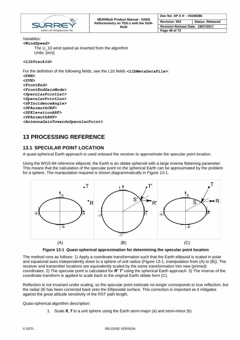
MERRByS Product Manual - GNSS Reflectometry on TDS-1 with the SGR-
ReSI
Doc No: XP X H - #0248366
Revision: 003 Status: Released
Revision Release Date: 19/07/2017
Page 49 of 73
© SSTL RELEASE VERSION
Variables: <WindSpeed>
The U_10 wind speed as inverted from the algorithm Units: [m/s]
<L1bTrackId>
For the definition of the following fields, see the L1b fields <L1bMetaDataFile>: <PRN>
<SVN>
<FrontEnd>
<FrontEndGainMode>
<SpecularPointLat>
<SpecularPointLon>
<SPIncidenceAngle>
<SPAzimuthORF>
<SPElevationARF>
<SPAzimuthARF>
<AntennaGainTowardsSpecularPoint>
13 PROCESSING REFERENCE
13.1 SPECULAR POINT LOCATION
A quasi-spherical Earth approach is used onboard the receiver to approximate the specular point location. Using the WGS-84 reference ellipsoid, the Earth is an oblate spheroid with a large inverse flattening parameter. This means that the calculation of the specular point on the spherical Earth can be approximated by the problem for a sphere. The manipulation required is shown diagrammatically in Figure 13-1.
Figure 13-1 Quasi-spherical approximation for determining the specular point location
The method runs as follows: 1) Apply a coordinate transformation such that the Earth ellipsoid is scaled in polar and equatorial axes independently down to a sphere of unit radius (Figure 13-1, manipulation from (A) to (B)). The receiver and transmitter locations are equivalently scaled by the same transformation into new (primed) coordinates. 2) The specular point is calculated for R’ T’ using the spherical Earth approach. 3) The inverse of the coordinate transform is applied to scale back to the original Earth oblate form (C). Reflection is not invariant under scaling, so the specular point estimate no-longer corresponds to true reflection, but the radial |𝑺| has been corrected back onto the Ellipsoidal surface. This correction is important as it mitigates against the great altitude sensitivity of the RST path length. Quasi-spherical algorithm description:
1. Scale R, T to a unit sphere using the Earth semi-major (a) and semi-minor (b)

MERRByS Product Manual - GNSS Reflectometry on TDS-1 with the SGR-
ReSI
Doc No: XP X H - #0248366
Revision: 003 Status: Released
Revision Release Date: 19/07/2017
Page 50 of 73
© SSTL RELEASE VERSION
Scaling matrix, 𝑭 =
[ 1
𝑎0 0
01
𝑎0
0 01
𝑏]
(13.1)
𝑹′ = 𝑭𝑹 , 𝑻′ = 𝑭𝑻 (13.2)
2. Determine the location of the specular point on the unit sphere, using spherical approach from [RD-
6 Martin-Neira 1993]. Call the solution, S’
3. Scale the solution back from the unit sphere to the original coordinate system
𝑺 = 𝑭−𝟏𝑺′ (13.3)
A Monte-Carlo analysis has been carried out to compare this approach to the solutions for the more accurate ellipsoidal Earth model. The analysis set covered a full range of receiver, transmitter and Earth geometries. The constraints on the simulation were a receiver at 500 km altitude, transmitter at 20,200 km altitude and only scenarios chosen where a specular point exists (transmitter being above the Earth limb by 1° elevation).
The reflection path length, 𝑅𝑆𝑇⃗⃗⃗⃗⃗⃗ ⃗⃗ , deviates from the correct Earth-ellipsoid solution by less than 15 m. The distance between estimates on the surface (Euclidean distance) is less than 3 km, which is within the 1st-iso range footprint on the surface and corresponds to a Doppler error of less than 200 Hz. The localization error is within a fraction of the scale of the ambiguity function in delay and Doppler so is acceptably small for reflection tracking. The specular points are located using this algorithm in the L1b products. If required, the DDMs can be retracked on the ground by recalculating the specular point location on the ellipsoid, geoid or elevation model as required.
13.2 SATELLITE ATTITUDE AND ANTENNA GAIN
13.2.1 Attitude reference frames
The orbit-defined coordinate system is a system of coordinates that maintains its orientation relative to the Earth as
the spacecraft moves in its orbit. An orthogonal triad of vectors, denoted X , Y and Z defines the reference
axes in the orbit-defined coordinate system. This is obtained from the receiver position and velocity in non-inertial, ECEF coordinates,WGS-84, therefore need a transformation due to the rotating frame using the Earth rotation vector,
0
0
eW
where is the Earth rotation rate, 7.2921158553e-5, rad/s
The inertial velocity is,
PWVVI e
where P and V are the ECEF receiver position and velocity respectively. The Y or pitch axis is directed toward
the negative orbit normal,
I
I
VP
VPY
13-1

MERRByS Product Manual - GNSS Reflectometry on TDS-1 with the SGR-
ReSI
Doc No: XP X H - #0248366
Revision: 003 Status: Released
Revision Release Date: 19/07/2017
Page 51 of 73
© SSTL RELEASE VERSION
The Z or yaw axis, is directed towards the centre of the Earth (nadir)
P
PZ
13-2
The X or roll axis completes the orthogonal set as the along-track vector,
ZYX 13-3
A second set of vectors, X , Y , Z define a second coordinate system termed the body-fixed coordinate
system that is defined relative to the spacecraft body itself. The attitude terms, roll, pitch and yaw are defined as
right-handed rotations about the three orbit-defined axes, with roll corresponding to a rotation about the X axis,
pitch a rotation about the Y axis and yaw a rotation about the Z axis.
Figure 13-2 Coordinate system definition
The attitude of the spacecraft is the orientation of the body-fixed coordinate system relative to the orbit-defined coordinate system.
13.2.2 Attitude representations
A common method for describing the attitude of a rigid body is the direct cosine matrix or attitude matrix. This
matrix is a coordinate transformation matrix that maps vectors from the reference frame to the body frame. If Oa is
a vector with components 1a , 2a , and 3a in the orbit-defined coordinate system, then
B
3
2
1
321
321
321
O aAa
w
v
u
a
a
a
a
a
a
www
vvv
uuu
13-4
where Ba is the same vector in body-fixed coordinates.
Orbit-defined coordinate system
Body-fixed coordinate system
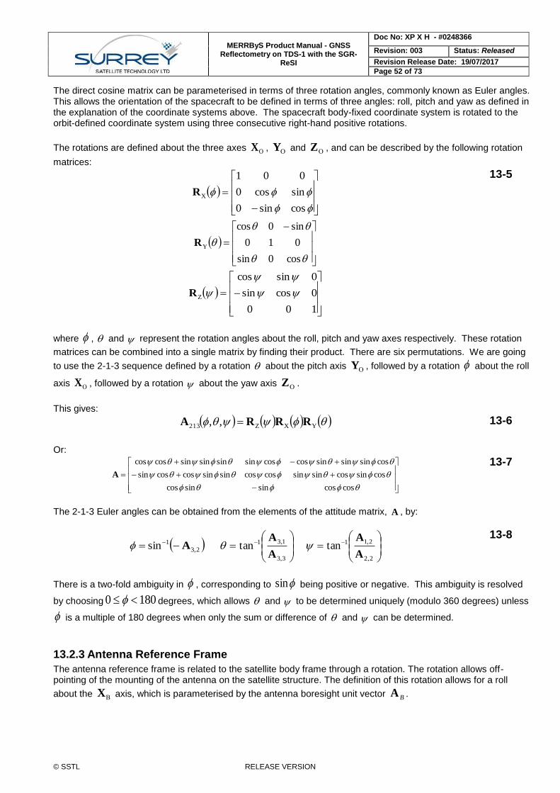
MERRByS Product Manual - GNSS Reflectometry on TDS-1 with the SGR-
ReSI
Doc No: XP X H - #0248366
Revision: 003 Status: Released
Revision Release Date: 19/07/2017
Page 52 of 73
© SSTL RELEASE VERSION
The direct cosine matrix can be parameterised in terms of three rotation angles, commonly known as Euler angles. This allows the orientation of the spacecraft to be defined in terms of three angles: roll, pitch and yaw as defined in the explanation of the coordinate systems above. The spacecraft body-fixed coordinate system is rotated to the orbit-defined coordinate system using three consecutive right-hand positive rotations.
The rotations are defined about the three axes X , Y and Z , and can be described by the following rotation
matrices:
cossin0
sincos0
001
XR
cos0sin
010
sin0cos
YR
100
0cossin
0sincos
Z
R
13-5
where , and represent the rotation angles about the roll, pitch and yaw axes respectively. These rotation
matrices can be combined into a single matrix by finding their product. There are six permutations. We are going
to use the 2-1-3 sequence defined by a rotation about the pitch axis Y , followed by a rotation about the roll
axis X , followed by a rotation about the yaw axis Z .
This gives:
YXZ213 ,, RRRA 13-6
Or:
coscossinsincos
cossincossinsincoscossinsincoscossin
cossinsinsincoscossinsinsinsincoscos
A
13-7
The 2-1-3 Euler angles can be obtained from the elements of the attitude matrix, A , by:
2,3
1sin A
3,3
1,31tanA
A
2,2
2,11tanA
A
13-8
There is a two-fold ambiguity in , corresponding to sin being positive or negative. This ambiguity is resolved
by choosing 1800 degrees, which allows and to be determined uniquely (modulo 360 degrees) unless
is a multiple of 180 degrees when only the sum or difference of and can be determined.
13.2.3 Antenna Reference Frame
The antenna reference frame is related to the satellite body frame through a rotation. The rotation allows off-pointing of the mounting of the antenna on the satellite structure. The definition of this rotation allows for a roll
about the X axis, which is parameterised by the antenna boresight unit vector BA .
MERRByS Product Manual - GNSS Reflectometry on TDS-1 with the SGR-
ReSI
Doc No: XP X H - #0248366
Revision: 003 Status: Released
Revision Release Date: 19/07/2017
Page 53 of 73
© SSTL RELEASE VERSION
This coordinate transformation matrix, RA , maps vectors from the body frame to the antenna reference frame. The
antenna reference frame is defined as the right-handed orthogonal frame consisting of the basis vectors: AX
which is the same as the body-frame X , AZ which is the antenna boresight vector, BA , and completing the set,
AY which is the vector XABv
If Ba is a vector with components 1a , 2a , and 3a in the body frame, then the rotation
A
3
2
1
321
321B
001
aaA
w
v
u
BBB
R
a
a
a
a
a
a
AAA
vvv
13-9
gives Aa , which is the same vector in the antenna reference frame, with components , , and
The antenna boresight for TDS-1 is along the axis,
Therefore the antenna reference frame is equivalent to the satellite body frame. To determine the antenna gain related to a particular vector, an Antenna Gain Map (AGM) look-up table is indexed
into using the vector’s azimuth and elevation. For example, the vector , in the antenna reference frame has
azimuth angle from the AX axis towards the AY axis.
)/tan( uvA aa 13-10
Where azimuth, A , is taken from -180 to 180 degrees.
Elevation is the angle between the vector and the AZ axis,
)/sin( awA a 13-11
13.3 DELAY DOPPLER MAP
13.3.1 DDM Scale
The DDM processing window is targeted to the specular point using open-loop tracking. The specular point location is calculated onboard and this is used to determine the delay and Doppler targeted by the DDM window. This is open-loop as information from the DDM pixels is not fed back to keep the reflection aligned with the tracking point. The purpose of the reflection targeting is to keep the specular point at a constant, defined, tracking offset in the DDM window. This tracking point is configurable in the receiver, so is reported in the <L1bMetadata,
Attributes>.
Delay:
ua va wa
Z
1
0
0
BA
Aa
MERRByS Product Manual - GNSS Reflectometry on TDS-1 with the SGR-
ReSI
Doc No: XP X H - #0248366
Revision: 003 Status: Released
Revision Release Date: 19/07/2017
Page 54 of 73
© SSTL RELEASE VERSION
If the DDM has delay pixels numbered with index, d, from 0 to <NumberOfDelayPixels-1>. Then the delay
scale can be calculated as: (Delay in samples) =
d * <CodeDelaySpacingSamplesBetweenPixels [samples / pixel]>
(Delay in seconds) =
(Delay in samples) / <SamplingFrequency [Hz]>
These give the delay scale from the first row of the DDM. The location of the tracking point is then defined on this scale as:
(Delay of tracking point in seconds) =
(<TrackingOffsetDelayNs> – <SpecularPathRangeOffset [ns]>) × 𝟏𝟎−𝟗
Where <TrackingOffsetDelayNs> is defined once for a whole track in <TrackMetaDataFile, Header>
and the field <SpecularPathRangeOffset> is defined per DDM in <TrackMetaDataFile, Data Array>.
This can alternatively be expressed in as the pixel offset from delay row 1. This is in <TrackingOffsetDelayInPixels>, which is calculated as:
(Delay Offset of Tracking Point) =
(<TrackingOffsetDelayNs [ns]> / <DelayResolution [ns/pixel]> )
(Delay Offset of Tracking Point Corrected)
= (Delay Offset of Tracking Point)
- (<SpecularPathRangeOffset[ns]> / <DelayResolution [ns/pixel]>)
Note that as this is an offset from pixel 1, a value of 64 in <TrackingOffsetDelayInPixels> corresponds to
the 65th delay row. Doppler: For the Doppler scale, the Doppler pixels are indexed D
from –floor(<NumberOfDopplerPixels> / 2) to + floor((<NumberOfDopplerPixels> - 0.5 ) / 2)
e.g. for 20 pixels:
-10, -9, -8, -7, -6, -5, -4, -3, -2, -1, 0, 1, 2, 3, 4, 5, 6, 7, 8, 9 The Doppler scale is then, (Doppler in Hz) =
D × <DopplerResolution> - <TrackingOffsetDopplerHz>
Alternatively the column, D, targeted is found from: (Doppler column from tracking point) =
D - <TrackingOffsetDopplerInPixels>
Power: The DDM pixels are the raw counts from the ZTC unit. Due to the scaling in the processor, these are an arbitrary ‘counts’ unit. The scaling does not change
13.4 ADC METRICS
We use different metrics to measure the quantisation of the front-end ADC sample distributions. These are defined here, and then these metrics are shown for the various SGR-ReSI boards.
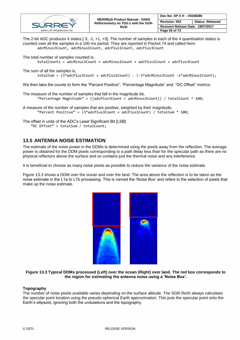
MERRByS Product Manual - GNSS Reflectometry on TDS-1 with the SGR-
ReSI
Doc No: XP X H - #0248366
Revision: 003 Status: Released
Revision Release Date: 19/07/2017
Page 55 of 73
© SSTL RELEASE VERSION
The 2-bit ADC produces 4 states [-3, -1, +1, +3]. The number of samples in each of the 4 quantisation states is counted over all the samples in a 100 ms period. They are reported in Packet 74 and called here:
adcMinus3Count, adcMinus1Count, adcPlus1Count, adcPlus3Count The total number of samples counted is,
totalCounts = adcMinus3Count + adcMinus1Count + adcPlus1Count + adcPlus3Count The sum of all the samples is,
totalSum = (3*adcPlus3Count + adcPlus1Count) - (-3*adcMinus3Count -1*adcMinus1Count); We then take the counts to form the “Percent Positive”, “Percentage Magnitude” and “DC Offset” metrics. The measure of the number of samples that fall in the magnitude bit,
“Percentage Magnitude” = ((adcPlus3Count + adcMinus3Count)) / totalCount * 100; A measure of the number of samples that are positive, weighted by their magnitude,
“Percent Positive” = (3*adcPlus3Count + adcPlus1Count) / totalSum * 100; The offset in units of the ADC’s Least Significant Bit [LSB]
“DC Offset” = totalSum / totalCount;
13.5 ANTENNA NOISE ESTIMATION
The estimate of the noise power in the DDMs is determined using the pixels away from the reflection. The average power is obtained for the DDM pixels corresponding to a path delay less than for the specular path as there are no physical reflectors above the surface and so contains just the thermal noise and any interference. It is beneficial to choose as many noise pixels as possible to reduce the variance of the noise estimate. Figure 13.3 shows a DDM over the ocean and over the land. The area above the reflection is to be taken as the noise estimate in the L1a to L1b processing. This is named the ‘Noise Box’ and refers to the selection of pixels that make up the noise estimate.
Figure 13.3 Typical DDMs processed (Left) over the ocean (Right) over land. The red box corresponds to the region for estimating the antenna noise using a ‘Noise Box’.
Topography The number of noise pixels available varies depending on the surface altitude. The SGR-ReSI always calculates the specular point location using the pseudo-spherical Earth approximation. This puts the specular point onto the Earth’s ellipsoid, ignoring both the undulations and the topography.
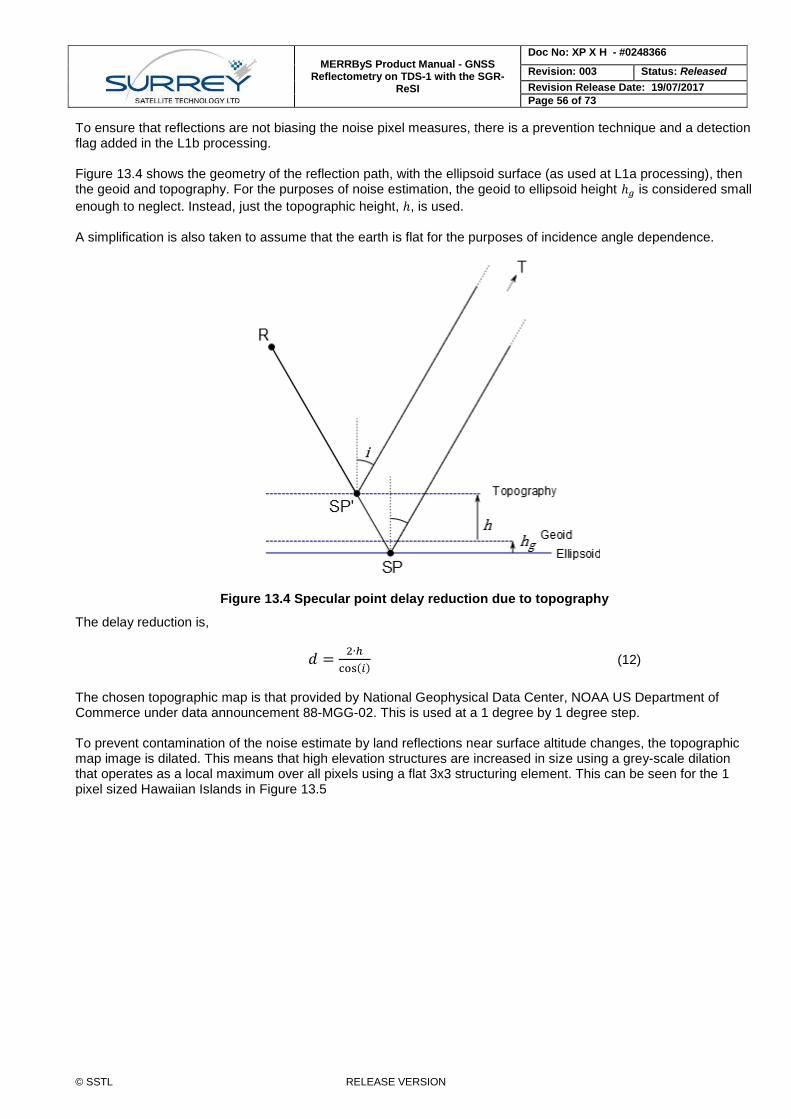
MERRByS Product Manual - GNSS Reflectometry on TDS-1 with the SGR-
ReSI
Doc No: XP X H - #0248366
Revision: 003 Status: Released
Revision Release Date: 19/07/2017
Page 56 of 73
© SSTL RELEASE VERSION
To ensure that reflections are not biasing the noise pixel measures, there is a prevention technique and a detection flag added in the L1b processing. Figure 13.4 shows the geometry of the reflection path, with the ellipsoid surface (as used at L1a processing), then the geoid and topography. For the purposes of noise estimation, the geoid to ellipsoid height ℎ𝑔 is considered small
enough to neglect. Instead, just the topographic height, ℎ, is used. A simplification is also taken to assume that the earth is flat for the purposes of incidence angle dependence.
Figure 13.4 Specular point delay reduction due to topography
The delay reduction is,
𝑑 =2∙ℎ
cos(𝑖) (12)
The chosen topographic map is that provided by National Geophysical Data Center, NOAA US Department of Commerce under data announcement 88-MGG-02. This is used at a 1 degree by 1 degree step. To prevent contamination of the noise estimate by land reflections near surface altitude changes, the topographic map image is dilated. This means that high elevation structures are increased in size using a grey-scale dilation that operates as a local maximum over all pixels using a flat 3x3 structuring element. This can be seen for the 1 pixel sized Hawaiian Islands in Figure 13.5
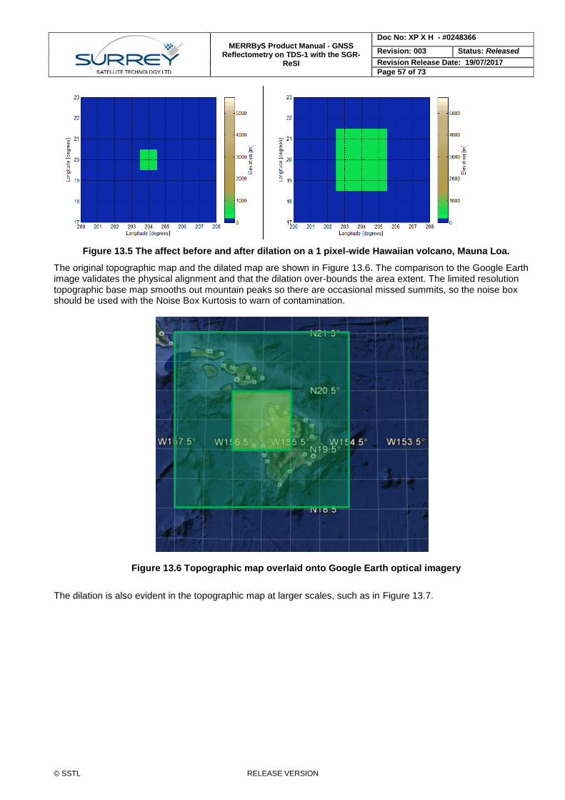
MERRByS Product Manual - GNSS Reflectometry on TDS-1 with the SGR-
ReSI
Doc No: XP X H - #0248366
Revision: 003 Status: Released
Revision Release Date: 19/07/2017
Page 57 of 73
© SSTL RELEASE VERSION
Figure 13.5 The affect before and after dilation on a 1 pixel-wide Hawaiian volcano, Mauna Loa.
The original topographic map and the dilated map are shown in Figure 13.6. The comparison to the Google Earth image validates the physical alignment and that the dilation over-bounds the area extent. The limited resolution topographic base map smooths out mountain peaks so there are occasional missed summits, so the noise box should be used with the Noise Box Kurtosis to warn of contamination.
Figure 13.6 Topographic map overlaid onto Google Earth optical imagery
The dilation is also evident in the topographic map at larger scales, such as in Figure 13.7.
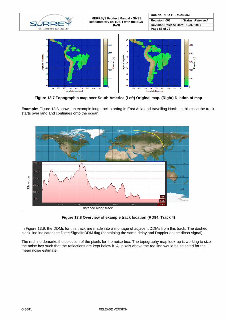
MERRByS Product Manual - GNSS Reflectometry on TDS-1 with the SGR-
ReSI
Doc No: XP X H - #0248366
Revision: 003 Status: Released
Revision Release Date: 19/07/2017
Page 58 of 73
© SSTL RELEASE VERSION
Figure 13.7 Topographic map over South America (Left) Original map. (Right) Dilation of map
Example: Figure 13.8 shows an example long track starting in East Asia and travelling North. In this case the track starts over land and continues onto the ocean.
.
Figure 13.8 Overview of example track location (RD84, Track 4)
In Figure 13.9, the DDMs for this track are made into a montage of adjacent DDMs from this track. The dashed black line indicates the DirectSignalInDDM flag (containing the same delay and Doppler as the direct signal). The red line demarks the selection of the pixels for the noise box. The topography map look-up is working to size the noise box such that the reflections are kept below it. All pixels above the red line would be selected for the mean noise estimate.
Distance along track
Ele
vat
ion
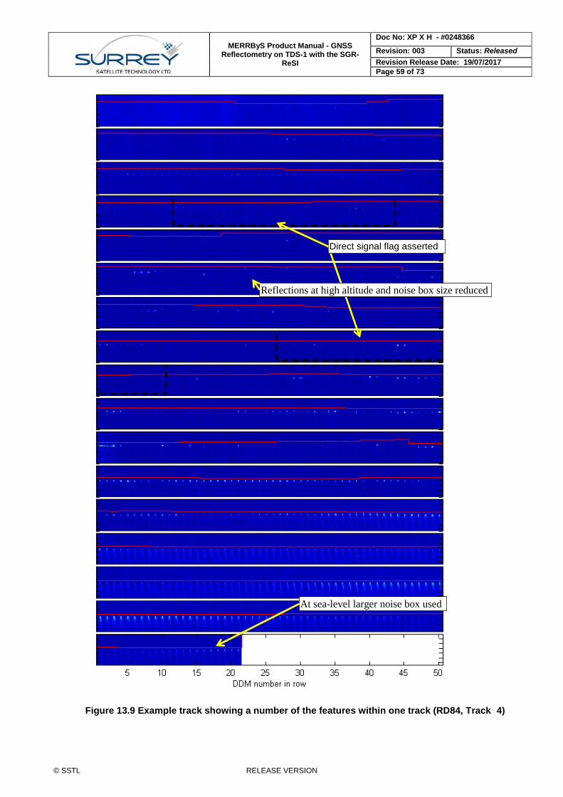
MERRByS Product Manual - GNSS Reflectometry on TDS-1 with the SGR-
ReSI
Doc No: XP X H - #0248366
Revision: 003 Status: Released
Revision Release Date: 19/07/2017
Page 59 of 73
© SSTL RELEASE VERSION
Figure 13.9 Example track showing a number of the features within one track (RD84, Track 4)
Direct signal flag asserted
At sea-level larger noise box used
Reflections at high altitude and noise box size reduced
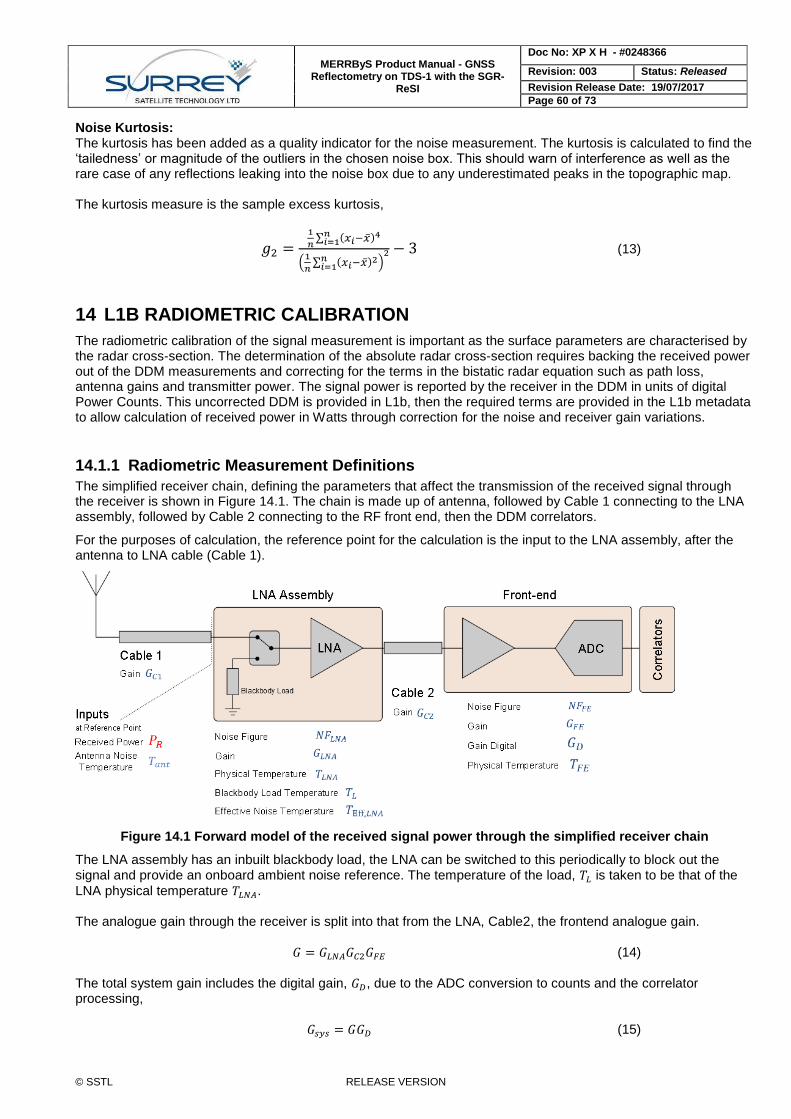
MERRByS Product Manual - GNSS Reflectometry on TDS-1 with the SGR-
ReSI
Doc No: XP X H - #0248366
Revision: 003 Status: Released
Revision Release Date: 19/07/2017
Page 60 of 73
© SSTL RELEASE VERSION
Noise Kurtosis: The kurtosis has been added as a quality indicator for the noise measurement. The kurtosis is calculated to find the ‘tailedness’ or magnitude of the outliers in the chosen noise box. This should warn of interference as well as the rare case of any reflections leaking into the noise box due to any underestimated peaks in the topographic map. The kurtosis measure is the sample excess kurtosis,
𝑔2 =1
𝑛∑ (𝑥𝑖−�̅�)4𝑛
𝑖=1
(1
𝑛∑ (𝑥𝑖−�̅�)2𝑛
𝑖=1 )2 − 3 (13)
14 L1B RADIOMETRIC CALIBRATION
The radiometric calibration of the signal measurement is important as the surface parameters are characterised by the radar cross-section. The determination of the absolute radar cross-section requires backing the received power out of the DDM measurements and correcting for the terms in the bistatic radar equation such as path loss, antenna gains and transmitter power. The signal power is reported by the receiver in the DDM in units of digital Power Counts. This uncorrected DDM is provided in L1b, then the required terms are provided in the L1b metadata to allow calculation of received power in Watts through correction for the noise and receiver gain variations.
14.1.1 Radiometric Measurement Definitions
The simplified receiver chain, defining the parameters that affect the transmission of the received signal through the receiver is shown in Figure 14.1. The chain is made up of antenna, followed by Cable 1 connecting to the LNA assembly, followed by Cable 2 connecting to the RF front end, then the DDM correlators.
For the purposes of calculation, the reference point for the calculation is the input to the LNA assembly, after the antenna to LNA cable (Cable 1).
Figure 14.1 Forward model of the received signal power through the simplified receiver chain
The LNA assembly has an inbuilt blackbody load, the LNA can be switched to this periodically to block out the signal and provide an onboard ambient noise reference. The temperature of the load, 𝑇𝐿 is taken to be that of the
LNA physical temperature 𝑇𝐿𝑁𝐴. The analogue gain through the receiver is split into that from the LNA, Cable2, the frontend analogue gain. 𝐺 = 𝐺𝐿𝑁𝐴𝐺𝐶2𝐺𝐹𝐸 (14) The total system gain includes the digital gain, 𝐺𝐷, due to the ADC conversion to counts and the correlator processing, 𝐺𝑠𝑦𝑠 = 𝐺𝐺𝐷 (15)

MERRByS Product Manual - GNSS Reflectometry on TDS-1 with the SGR-
ReSI
Doc No: XP X H - #0248366
Revision: 003 Status: Released
Revision Release Date: 19/07/2017
Page 61 of 73
© SSTL RELEASE VERSION
As the reference point is after Cable 1, it’s gain/loss, 𝐺𝐶1 is not included.
14.1.2 Receiver Measurements
Signal measurements: The analogue received signal power at the ADC input is, 𝑃 = 𝑃𝑅𝐺 (16) The digital measurement after correlation is the DDM pixel. This is a measure in units of DDM Power Counts, (sometimes just Counts for short). The matched filter in the DDM accepts the signal, but additionally it accepts any noise (thermal or interference) in the filter bandwidth. The measurement is a DDM pixel (𝑃∗), in units of DDM Power Counts, is subject to digital scaling and implementation loss. 𝑃∗ = 𝐺𝐷(𝐿𝑆𝑃 + 𝐿𝑁𝑁) (17) Separate implementation losses are used for signal and noise and use the definition,
𝑆𝑁𝑅
𝑆𝑁𝑅𝑖𝑑𝑒𝑎𝑙=
𝐿𝑆
𝐿𝑁 (18)
The implementation loss, 𝐿𝑆 𝐿𝑁⁄ , is dependent on the non-linear effects, such as clipping, in the 2-bit ADC. It depends on the total noise power incident on the ADC, so we define multiple 𝐿𝑁… terms, one for each measurement. The value assigned is defined in section 14.1.4. Noise measurements (antenna): The receiver can measure the noise after correlation from the antenna by using the DDM pixels away from the reflection. The analogue received noise power at ADC input is, for the antenna, 𝑁 = 𝑘𝐵(𝑇𝑎𝑛𝑡 + 𝑇𝑟𝑥)𝐺 (19) The measurement is a DDM pixel, in units of Power Counts, is subject to digital scaling and implementation loss. 𝑁∗ = 𝐺𝐷𝐿𝑁𝑁 (20) Noise measurements (blackbody): The receiver can measure the noise after correlation of the blackbody using all the DDM pixels, as there is no signal present. The analogue received noise power at ADC input is, for the blackbody, 𝑁𝐿 = 𝑘𝐵(𝑇𝐿 + 𝑇𝑟𝑥)𝐺 (21) The measurement is a DDM pixel, in units of Power Counts, is subject to digital scaling and implementation loss.
𝑁𝐿∗ = 𝐺𝐷𝐿𝑁,𝐿𝑁𝐿 (22)
Where the implementation loss (𝐿𝑁,𝐿) has an added sub-script (L) for the measurement with the blackbody load.
The loss is dependent on the input power level, and so different from that measured with the antenna, 𝐿𝑁.
14.1.3 Derived Measurements
From these basic low-level observables, further measurements can be derived. System Gain:
MERRByS Product Manual - GNSS Reflectometry on TDS-1 with the SGR-
ReSI
Doc No: XP X H - #0248366
Revision: 003 Status: Released
Revision Release Date: 19/07/2017
Page 62 of 73
© SSTL RELEASE VERSION
The receiver system gain can vary, primarily due to changes in physical temperature of the receiver. However it could also change due to radiation induced aging of the receiver amplifiers. It is therefore important that this can be measured onboard. The gain can be measured using the LNA’s internal blackbody or an external reference. The gain in the system can be found from rearranging the noise measurement of the blackbody reference, 𝑁𝐿
∗:
𝐺𝐺𝐷 =𝑁𝐿
∗
𝐿𝑁,𝐿∙𝑘𝐵(𝑇𝐿+𝑇𝑟𝑥) (23)
This provides the conversion from DDM Power Counts to Watts. Likewise if the antenna is pointed to an External Source with known temperature 𝑇ExtRef, then the gain can be
calculated from the DDM measurement, 𝑁ExtRef∗ , as:
𝐺𝐺𝐷 =𝑁ExtRef
∗
𝐿𝑁,ExtRef∙𝑘𝐵(𝑇ExtRef+𝑇𝑟𝑥) (24)
Both measurements, from blackbody and external reference are available in the L1b metadata when available.
Gain temperature compensation The temperature dependence of the gain is dominated by the LNA. Using this knowledge, the gain can be extrapolated from a measurement at one physical temperature to another. The gain from the LNA (in dB units) is well modelled by a linear function of physical temperature,
𝐺𝐿𝑁𝐴 = 10(𝑔𝑐+𝑔𝑚𝑇𝐿𝑁𝐴)
10 (25)
Using the convention that 𝑔 is for gain in dB, and is a linear function with offset 𝑔𝑐 and gradient 𝑔𝑚. The extrapolation can be performed by using the ratio of gain measurement taken with blackbody at LNA
temperature 𝑇𝐿𝑁𝐴,𝐿, to the temperature when the reflection DDM is measured, 𝑇𝐿𝑁𝐴,𝑅,
𝐺𝐿𝑁𝐴|𝑇𝐿𝑁𝐴,𝑅
𝐺𝐿𝑁𝐴|𝑇𝐿𝑁𝐴,𝐿
=10
(𝑔𝑐+𝑔𝑚𝑇𝐿𝑁𝐴,𝑅)10
10(𝑔𝑐+𝑔𝑚𝑇𝐿𝑁𝐴,𝐿)
10
𝐺𝐿𝑁𝐴|𝑇𝐿𝑁𝐴,𝑅= 10
(𝑔𝑐+𝑔𝑚𝑇𝐿𝑁𝐴,𝑅)10
−(𝑔𝑐+𝑔𝑚𝑇𝐿𝑁𝐴,𝐿)
10 𝐺𝐿𝑁𝐴|𝑇𝐿𝑁𝐴,𝐿
𝐺𝐿𝑁𝐴|𝑇𝐿𝑁𝐴,𝑅= 10
𝑔𝑚(𝑇𝐿𝑁𝐴,𝑅−𝑇𝐿𝑁𝐴,𝐿)
10 𝐺𝐿𝑁𝐴|𝑇𝐿𝑁𝐴,𝐿 (26)
Likewise for the external reference the gain compensation is,
𝐺𝐿𝑁𝐴|𝑇𝐿𝑁𝐴,𝑅= 10
𝑔𝑚(𝑇𝐿𝑁𝐴,𝑅−𝑇𝐿𝑁𝐴,ExtRef)
10 𝐺𝐿𝑁𝐴|𝑇𝐿𝑁𝐴,ExtRef (27)
This uses only the rate of change of gain with temperature, which can be taken from the pre-launch ground based LNA testing, or can be re-measured in-orbit using measurements with the blackbody. Antenna Noise Temperature: The antenna noise power can be found from dividing the noise power measurements from the antenna by those from the blackbody,
𝑁∗
𝑁𝐿∗ =
𝑘𝐵(𝑇𝑎𝑛𝑡+𝑇𝑟𝑥)𝐺𝐺𝐷𝐿𝑁
𝑘𝐵(𝑇𝐿+𝑇𝑟𝑥)𝐺𝐺𝐷𝐿𝑁,𝐿 (28)
MERRByS Product Manual - GNSS Reflectometry on TDS-1 with the SGR-
ReSI
Doc No: XP X H - #0248366
Revision: 003 Status: Released
Revision Release Date: 19/07/2017
Page 63 of 73
© SSTL RELEASE VERSION
However as the measurement of the blackbody is not simultaneous to that of the blackbody it is useful to split out
how these terms are defined at their measurement times. The antenna is measured at LNA temperature 𝑇𝐿𝑁𝐴,𝑅 and
the blackbody load at temperature 𝑇𝐿𝑁𝐴,𝐿. This results in separate receiver noise temperature, 𝑇𝑟𝑥|𝑇𝐿𝑁𝐴,𝑅, 𝑇𝑟𝑥|𝑇𝐿𝑁𝐴,𝐿
and receiver gain, 𝐺|𝑇𝐿𝑁𝐴,𝑅, 𝐺|𝑇𝐿𝑁𝐴,𝐿
.
𝑁∗
𝑁𝐿∗ =
𝑘𝐵(𝑇𝑎𝑛𝑡+𝑇𝑟𝑥|𝑇𝐿𝑁𝐴,𝑅)𝐺|𝑇𝐿𝑁𝐴,𝑅
𝐺𝐷𝐿𝑁
𝑘𝐵(𝑇𝐿+𝑇𝑟𝑥|𝑇𝐿𝑁𝐴,𝐿)𝐺|𝑇𝐿𝑁𝐴,𝐿
𝐺𝐷𝐿𝑁,𝐿 (29)
Rearranging for T𝑎𝑛t, and using the linear gain temperature compensation this becomes,
𝑇𝑎𝑛𝑡 =𝑁∗𝐿𝑁,𝐿
𝑁𝐿∗𝐿𝑁
10𝑔𝑚(𝑇𝐿𝑁𝐴,𝑅−𝑇𝐿𝑁𝐴,𝐿)
10 (𝑇𝐿 + 𝑇𝑟𝑥|𝑇𝐿𝑁𝐴,𝐿) − 𝑇𝑟𝑥|𝑇𝐿𝑁𝐴,𝑅
(30)
Likewise when using the external reference, this is:
Tant =N∗LN,ExtRef
NExtRef∗ LN
10gm(TLNA,R−TLNA,ExtRef)
10 (TExtRef + Trx|TLNA,ExtRef) − Trx|TLNA,R
(31)
Both measurements, from blackbody and external reference are available in the L1b metadata when available.
Received Power The received power can be measured from either of two formulations of the above observables, either from correcting the Signal to Noise Ratio (SNR), or applying the gain measurement to the digital Signal Minus Noise (SMN). Corrected SNR The digital SNR is calculated as follows:
SNR = Γ =P∗−N∗
N∗ =P∗
N∗ − 1 (32)
Substituting in the analogue constituents, this becomes,
𝑆𝑁𝑅 =𝐿𝑆∙𝑃𝑅𝐺𝐺𝐷
𝐿𝑁𝑘𝐵(𝑇𝑎𝑛𝑡+𝑇𝑟𝑥)𝐺𝐺𝐷− 1 =
𝐿𝑆∙𝑃𝑅
𝐿𝑁𝑘𝐵(𝑇𝑎𝑛𝑡+𝑇𝑟𝑥)− 1 (33)
The receiver gain cancels out, but remaining are the antenna and system noise power. Rearranging for received power, this effectively becomes a correction to the digital SNR,
𝑃𝑅 = (𝑃∗
𝑁∗ − 1)𝐿𝑁𝑘𝐵(𝑇𝑎𝑛𝑡+𝑇𝑟𝑥)
𝐿𝑆 (34)
Corrected SMN An alternative formulation is the correction of the Signal Minus Noise digital measure: SMN = 𝑃∗ − 𝑁∗ (35) Substituting in the analogue constituents, prior to the ADC, this becomes,
SMN = 𝐺𝐷(𝐿𝑆𝑃 + 𝐿𝑁𝑁) − 𝐺𝐷𝐿𝑁𝑁
= 𝐺𝐷𝐿𝑆𝑃 (36) Substituting in the analogue parts and rearranging this for the received power,
MERRByS Product Manual - GNSS Reflectometry on TDS-1 with the SGR-
ReSI
Doc No: XP X H - #0248366
Revision: 003 Status: Released
Revision Release Date: 19/07/2017
Page 64 of 73
© SSTL RELEASE VERSION
𝑃𝑅 =𝑃
𝐺=
SMN
𝐺𝐺𝐷𝐿𝑆 (37)
Both routes to calculating the received power produce exactly the same value. Receiver Noise Temperature Calculation <RxTemperature> The receiver noise temperature is calculated using the Friis cascade of noise temperature through the system using the component values measured prior to launch. The reference point is the LNA input, so does not include the antenna to LNA cable (C1). The calculation of RxTemperature uses the radiometric characterisation data, which is corrected to the physical temperature of the LNA, 𝑇𝐿𝑁𝐴. The cascaded receiver noise temperature is,
𝑇𝑟𝑥 = 𝑇Eff,𝐿𝑁𝐴 +𝑇𝐶2
𝐺𝐿𝑁𝐴+
𝑇𝐹𝐸
𝐺𝐿𝑁𝐴𝐺𝐶2 (38)
where 𝑇Eff,𝐿𝑁𝐴, 𝑇𝐶2 and 𝑇𝐹𝐸 are the effective noise temperatures of the LNA, Cable 2 and front-end. The gain terms
are for the LNA, 𝐺𝐿𝑁𝐴 and for Cable 2, 𝐺𝐶2. LNA Noise figure The noise figure of the LNA is calculated from a look-up function with physical temperature, 𝑇𝐿𝑁𝐴. This look-up is from linear regression of the pre-launch LNA noise figure in units of dB. 𝑁𝐹𝐿𝑁𝐴 = 𝐶 + 𝑚𝑇𝐿𝑁𝐴 (39) The values from pre-launch testing of the nadir LNA are, 𝐶 = 2.328243
𝑚 = 0.011905 This is then converted into noise factor,
𝐹𝐿𝑁𝐴 = 10𝐶+𝑚𝑇𝐿𝑁𝐴
10 (40) Which is related to the effective noise temperature as, 𝑇Eff,𝐿𝑁𝐴 = 𝑇ref(𝐹𝐿𝑁𝐴 − 1) (41)
The temperature, 𝑇ref, is taken as 290 K. LNA Gain
The gain of the LNA is also calculated from look-up function with physical temperature, 𝑇𝐿𝑁𝐴. This look-up is from linear regression of the pre-launch LNA gain in units of dB. 𝑔𝐿𝑁𝐴 = 𝐶 + 𝑚𝑇𝐿𝑁𝐴 (42) This is then converted to linear scaling,
𝐺𝐿𝑁𝐴 = 10𝑔𝐿𝑁𝐴
10 (43)
The values from pre-launch testing of the nadir LNA are,
𝐶 = 27.843243
𝑚 = -0.034595
Cable losses For Cable 2 the effective temperature is,
𝑇𝐶2 = 𝑇𝐶2 (1
𝐺𝐶2− 1) (44)

MERRByS Product Manual - GNSS Reflectometry on TDS-1 with the SGR-
ReSI
Doc No: XP X H - #0248366
Revision: 003 Status: Released
Revision Release Date: 19/07/2017
Page 65 of 73
© SSTL RELEASE VERSION
Where 𝑇𝐶2 is the physical temperature of the cable. Front end
The noise figure for the front-end is taken from the data-sheet. Due to being divided by 𝐺𝐿𝑁𝐴𝐺𝐶2, it is small and the exact value is not significant. The assumed value is, 𝑇𝐹𝐸 = 𝑇ref(𝐹𝐹𝐸 − 1) (45) The noise figure is taken to be, 𝑁𝐹𝐹𝐸= -1.5 dB, and so Noise Factor 𝐹𝐹𝐸 = 0.7079 The flow of data from DDM basic to derived observables is shown in Figure 14.2, which indicates the flow of data into the metadata fields.
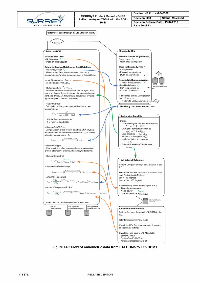
MERRByS Product Manual - GNSS Reflectometry on TDS-1 with the SGR-
ReSI
Doc No: XP X H - #0248366
Revision: 003 Status: Released
Revision Release Date: 19/07/2017
Page 66 of 73
© SSTL RELEASE VERSION
Figure 14.2 Flow of radiometric data from L1a DDMs to L1b DDMs

MERRByS Product Manual - GNSS Reflectometry on TDS-1 with the SGR-
ReSI
Doc No: XP X H - #0248366
Revision: 003 Status: Released
Revision Release Date: 19/07/2017
Page 67 of 73
© SSTL RELEASE VERSION
14.1.4 Implementation Loss Terms
The implementation loss terms are due to the 2-bit ADC providing a non-linear transfer from analogue to digital signal representations. The value is dependent on sampling frequency, filter bandwidth, total noise power, number of quantisation levels. The suggested value is the constant,
𝐿𝑆
𝐿𝑁= 1.3, or 1.1 dB (46)
There is a small variation dependent on the total noise power incident on the LNA. The implementation loss terms are used for the antenna temperature and system gain fields in the L1b metadata. However the implementation loss is effectively ignored as they are set to, 𝐿𝑆 = 1 and 𝐿𝑁 = 1 in the L1b version 0.7.

MERRByS Product Manual - GNSS Reflectometry on TDS-1 with the SGR-
ReSI
Doc No: XP X H - #0248366
Revision: 003 Status: Released
Revision Release Date: 19/07/2017
Page 68 of 73
© SSTL RELEASE VERSION
15 RELEASE NOTES
15.1 RELEASE NOTES FOR L1B V0.5
15.1.1 Changes from v0.3 to v0.5
1. Due to a number of the changes out-lined below, the storing of DDMs from L1a to L1b will have resulted in the tracks being renumbered. This is due to the track ID number being sequential and if a new track is created that did not exist in the previous version then all subsequent tracks will be renamed to make room in the sequence.
2. During reflection channel reallocation, the receiver switches from tracking one transmitter to another. The L1a to L1b processing stage now checks the data in SBPP packets before and after the reallocation in an improved method to reduce data loss.
3. Internally more statistics are recorded for determining the reasons why DDMs are excluded from the L1b .data
4. Added functionality to extract DDMs with LNA switched to the internal Blackbody. These blackbody DDMs are not included in the regular track files. This new file will be defined in the next release of the Product Manual.
5. Removed the averaging of noise over the track for calculating SNR. This noise is now calculated from one pixel (top pixel and 0 Hz Doppler). The reason for this change is that averaging of noise over time is not suitable when the AGC is turned on as the front-end gain can be changing. The signal and noise measures can be at different gains, so does represent the input SNR well.
6. Updated the Track Epoch <SpecularPathRangeOffset> for the tracking fix in v1.3 of the receiver application code. The tracking error that was reported in the L1b <SpecularPathRangeOffset> is applied onboard the satellite from RD21, therefore this correction term becomes zero.
7. DDM timestamps were off by 1 second. Previously the end-of-integration mistakenly marked as start-of-integration.
8. In <TrackMetaDataFile><TrackingMode> Enumeration names changed. Previously these were incorrect.
9. Fixed an issue with interpolation of the satellite attitude at the end of day (00:00:00)
10. The attitude of the satellite is now taken from the platform attitude solution. Previously the attitude source was set to NominalAttitudeAssumed rather than actually taking in the platform data. The attitude data needs to be used cautiously due to the different form of the errors from the sun-sensors and during eclipse, from the magnetometers. The measurements are the output of the Kalman filter which is used as feedback for the attitude control. As an example, an attitude measurement of (0,0,0) for (roll, pitch, yaw) means that the control system is steering the attitude to the nominal direction. However the measurement is still subject to the biases from the sensors. The best guess for the uncertainty is provided in the AttitudeUncertainty field.
11. The Eclipse flag was incorrect previously. This is used for determining the satellite attitude uncertainty. In v0.3 the eclipse flag was calculated given the receiver position and the time. The calculation was incorrect. The flag now uses the sun-sensor active flag from the onboard attitude control. The sun sensors are turned off just before eclipse and turned on again just after, to avoid atmospheric effects.
12. Added more data to the Track KMZ file

MERRByS Product Manual - GNSS Reflectometry on TDS-1 with the SGR-
ReSI
Doc No: XP X H - #0248366
Revision: 003 Status: Released
Revision Release Date: 19/07/2017
Page 69 of 73
© SSTL RELEASE VERSION
13. Orbit Reference Frame defined in Product Manual
14. Correction to attitude rotation matrix in Product Manual
15. Change to allow a higher loss rate of front-end status packets (and still consider the data to be valid) This contains LNA temperature and ADC Mag bit ratio.
16. Corrected the file naming convention of the attitude input files
15.1.2 Changes from v0.5 to v0.7
1. Changed data format from XML and TIFF to NetCDF4 for more effective file handling and better software library support.
2. Changed data naming conventions from RD number to date and time (yyyy-MM/dd/Hhh)
3. Added direct signal power measurements extraction to ‘directSignalPower.nc’
4. Added radiometric terms for calibration of the L1b data
Fill in new fields into Metadata: ReceiverMetaData: BlackbodyPower, SystemGainBB, SystemGainBBComp, SystemGainExtRef,
SystemGainExtRefComp, ReferenceType, RxTemperature, NadirRadiometricFrontendList TrackMetaData: (In Header)TagName, MeanNoiseHighDoppler, MeanNoiseBox,
KurtosisNoiseBox, NoiseBoxRows, DDMSNRAtPeakSingleDDM, AntennaTemperature, AntennaTemperatureExtRef
Improved noise estimate added to reduce estimation variance Added noise measure that selects DDM top pixels, adjusting number based on maximum
available depending on topography of the surface: ‘NoiseBox’. Added noise box Kurtosis measure Number of rows used reported in NoiseBoxRows. If none are available (Value 0) then can use
MeanNoiseHighDoppler as a fall-back which has greater altitude range by taking high Doppler pixels.
PeakSNR now uses this new noise measure Blackbody extraction:
Added extraction of the blackbody DDMs to files: blackbodyNadir.nc and blackbodyZenith.nc Antenna gain uncertainty field (AntennaGainRange) added to L1b Track Epochs
Propagation of uncertainty from attitude uncertainty
5. Bug fixes:
Timestamps issue corrected Timestamp steering whilst DDMs are being output caused rare occurrence of RD file time stamps
to be out of order. Now these DDMs are removed from L1b Occasional completion of tracks when no changes have occurred DirectSignalInDDM flag did not catch all cases and had a small offset Swapped the LNA temperature telemetry (Nadir / Zenith) that was the wrong way around for older
data Allow greater packet loss of ADC telemetry
6. Added field to ReceiverMetaData, TimeDifferenceToClosestPVT – this field may be useful for analysis of altimetry to determine whether the PVT was generated onboard or from interpolation on the ground.

MERRByS Product Manual - GNSS Reflectometry on TDS-1 with the SGR-
ReSI
Doc No: XP X H - #0248366
Revision: 003 Status: Released
Revision Release Date: 19/07/2017
Page 70 of 73
© SSTL RELEASE VERSION
7. Removed fields LandType and DDMPixelValueNoiseInvalid
8. Summary plots created to monitor data quality
9. Added TDS-1 yaw change of 180 degrees after 19/10/2016
10. Transmitter position has been propagated back to the time of transmission of the reflected signal, rather than time of reception. This effects a change in transmitter position of ~70 m.
Known issues:
In the file, DDMs.nc, in all the V0.7 Level 1B, the delay scale is off by one. The correct scale is given in section 13.3.1
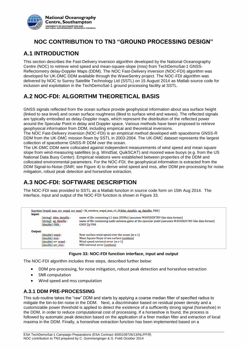
ESA TechDemoSat-1 Campaign Preparations (ESA Contract 4000109726/13/NL/FF/lf) NOC contribution to TN3 prepared by C. Gommenginger & G. Foti6 October 2014
NOC CONTRIBUTION TO TN3 “GROUND PROCESSING DESIGN”
A.1 INTRODUCTION
This section describes the Fast-Delivery inversion algorithm developed by the National Oceanography Centre (NOC) to retrieve wind speed and mean-square-slope (mss) from TechDemoSat-1 GNSS-Reflectometry delay-Doppler Maps (DDM). The NOC Fast-Delivery inversion (NOC-FDI) algorithm was developed for UK-DMC DDM available through the WaveSentry project. The NOC-FDI algorithm was delivered by NOC to Surrey Satellite Technology Ltd (SSTL) on 15 August 2014 as Matlab source code for inclusion and exploitation in the TechDemoSat-1 ground processing facility at SSTL.
A.2 NOC-FDI: ALGORITHM THEORETICAL BASIS
GNSS signals reflected from the ocean surface provide geophysical information about sea surface height (linked to sea level) and ocean surface roughness (liked to surface wind and waves). The reflected signals are typically embodied as delay-Doppler maps, which represent the distribution of the reflected power around the Specular Point in delay and Doppler space. Various methods have been proposed to retrieve geophysical information from DDM, including empirical and theoretical inversions. The NOC Fast-Delivery inversion (NOC-FDI) is an empirical method developed with spaceborne GNSS-R DDM from the UK-DMC mission flown by SSTL in 2003-2004. The UK-DMC dataset represents the largest collection of spaceborne GNSS-R DDM over the ocean. The UK-DMC DDM were collocated against independent measurements of wind speed and mean square slope from wind-measuring satellites (e.g. WindSat, QuikSCAT) and moored wave buoys (e.g. from the US National Data Buoy Center). Empirical relations were established between properties of the DDM and collocated environmental parameters. For the NOC-FDI, the geophysical information is extracted from the DDM Signal-to-Noise (SNR; see Figure 4) to derive wind speed and mss, after DDM pre-processing for noise mitigation, robust peak detection and horseshoe extraction.
A.3 NOC-FDI: SOFTWARE DESCRIPTION
The NOC-FDI was provided to SSTL as a Matlab function in source code form on 15th Aug 2014. The interface, input and output of the NOC-FDI function is shown in Figure 33.
Figure 33: NOC-FDI function interface, input and output
The NOC-FDI algorithm includes three steps, described further below:
DDM pre-processing, for noise mitigation, robust peak detection and horseshoe extraction
SNR computation
Wind speed and mss computation
A.3.1 DDM PRE-PROCESSING
This sub-routine takes the “raw” DDM and starts by applying a coarse median filter of specified radius to mitigate the bin-to-bin noise in the DDM. Next, a discriminator based on residual power density and a customizable power threshold is applied to detect the existence of a sufficiently strong signal (horseshoe) in the DDM, in order to reduce computational cost of processing. If a horseshoe is found, the process is followed by automatic peak detection based on the application of a finer median filter and extraction of local maxima in the DDM. Finally, a horseshoe extraction function has been implemented based on a
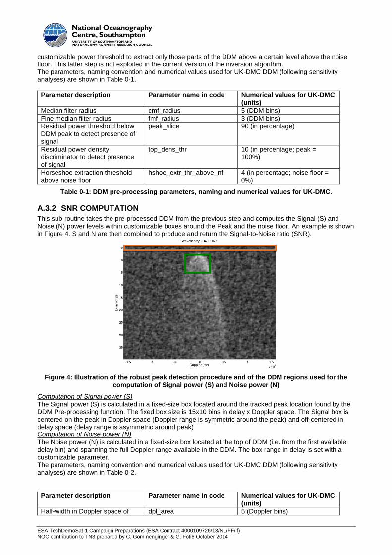
ESA TechDemoSat-1 Campaign Preparations (ESA Contract 4000109726/13/NL/FF/lf) NOC contribution to TN3 prepared by C. Gommenginger & G. Foti6 October 2014
customizable power threshold to extract only those parts of the DDM above a certain level above the noise floor. This latter step is not exploited in the current version of the inversion algorithm. The parameters, naming convention and numerical values used for UK-DMC DDM (following sensitivity analyses) are shown in Table 0-1.
Parameter description Parameter name in code Numerical values for UK-DMC (units)
Median filter radius cmf_radius 5 (DDM bins)
Fine median filter radius fmf_radius 3 (DDM bins)
Residual power threshold below DDM peak to detect presence of signal
peak_slice 90 (in percentage)
Residual power density discriminator to detect presence of signal
top_dens_thr 10 (in percentage; peak = 100%)
Horseshoe extraction threshold above noise floor
hshoe_extr_thr_above_nf 4 (in percentage; noise floor = 0%)
Table 0-1: DDM pre-processing parameters, naming and numerical values for UK-DMC.
A.3.2 SNR COMPUTATION
This sub-routine takes the pre-processed DDM from the previous step and computes the Signal (S) and Noise (N) power levels within customizable boxes around the Peak and the noise floor. An example is shown in Figure 4. S and N are then combined to produce and return the Signal-to-Noise ratio (SNR).
Figure 4: Illustration of the robust peak detection procedure and of the DDM regions used for the computation of Signal power (S) and Noise power (N)
Computation of Signal power (S) The Signal power (S) is calculated in a fixed-size box located around the tracked peak location found by the DDM Pre-processing function. The fixed box size is 15x10 bins in delay x Doppler space. The Signal box is centered on the peak in Doppler space (Doppler range is symmetric around the peak) and off-centered in delay space (delay range is asymmetric around peak) Computation of Noise power (N)
The Noise power (N) is calculated in a fixed-size box located at the top of DDM (i.e. from the first available delay bin) and spanning the full Doppler range available in the DDM. The box range in delay is set with a customizable parameter. The parameters, naming convention and numerical values used for UK-DMC DDM (following sensitivity analyses) are shown in Table 0-2.
Parameter description Parameter name in code Numerical values for UK-DMC (units)
Half-width in Doppler space of dpl_area 5 (Doppler bins)

ESA TechDemoSat-1 Campaign Preparations (ESA Contract 4000109726/13/NL/FF/lf) NOC contribution to TN3 prepared by C. Gommenginger & G. Foti6 October 2014
signal box around peak
Width in delay space of signal box above peak
del_area_above_peak 4 (delay bins)
Width in delay space of signal box below peak
del_area_below_peak 10 (delay bins)
Width in delay space of noise box from minimum delay in DDM
noise_area_size 20 (delay bins)
Table 0-2: SNR computation parameters, naming and numerical values for UK-DMC.
A.3.3 WIND SPEED AND MSS COMPUTATION
This sub-routine takes the SNR computed in the previous step, calculates the SNR corrected for the Antenna gain at the specular point (AGC_SNR), then applies the power-law relation developed from the UK-DMC/Windsat matchup dataset.
Parameter Units
Wind speed at 10 metres m/s
Mean-square slope No units
Wind speed uncertainty m/s
Mean-square slope uncertainty
No units
Table 0-3: Output parameters