Embed Size (px)
Citation preview
Mesoscopic Structure of Complex Networks
Ph.D. thesis
Gergely Tibely
supervisor:Prof. Janos Kertesz
Budapest University of Technology and EconomicsDepartment of Theoretical Physics
2011


Azoknak, akik hisznek abban, hogy a tudomany az
igazsag megismeresenek az eszkoze.
For the ones who believe that science and humani-
ties are for learning the truth.


Contents
1 Introduction 1
2 Complex networks in general 4
2.1 Definition and reach . . . . . . . . . . . . . . . . . . . . . . . 4
2.2 Anatomy of complex network research . . . . . . . . . . . . . 5
2.2.1 Fields of applications . . . . . . . . . . . . . . . . . . . 5
2.2.2 Lines of research . . . . . . . . . . . . . . . . . . . . . 8
2.3 Important concepts and results . . . . . . . . . . . . . . . . . 10
2.3.1 General results . . . . . . . . . . . . . . . . . . . . . . 10
2.3.2 Some application results from complex networks ingeneral . . . . . . . . . . . . . . . . . . . . . . . . . . 12
2.4 Tools . . . . . . . . . . . . . . . . . . . . . . . . . . . . . . . . 14
3 Introduction to community detection 16
3.1 Historical overview . . . . . . . . . . . . . . . . . . . . . . . . 16
3.2 Relation to statistical physics . . . . . . . . . . . . . . . . . . 18
3.3 Definition of the problem . . . . . . . . . . . . . . . . . . . . 20
3.4 Difficulties . . . . . . . . . . . . . . . . . . . . . . . . . . . . . 21
3.5 Other fields’ methods . . . . . . . . . . . . . . . . . . . . . . 25
3.6 Overview of the current methods . . . . . . . . . . . . . . . . 26
3.6.1 Random walk-based methods . . . . . . . . . . . . . . 26
3.6.2 Potts model-related methods . . . . . . . . . . . . . . 28
3.6.3 Percolation-related methods . . . . . . . . . . . . . . . 34
3.6.4 Other . . . . . . . . . . . . . . . . . . . . . . . . . . . 35
3.7 Results & applications so far . . . . . . . . . . . . . . . . . . 40
4 Analysis of a few community detection methods 42
4.1 Properties of the label propagation method . . . . . . . . . . 42
4.1.1 The zero-temperature kinetic Potts model . . . . . . . 43
4.1.2 Analysis of the label propagation method . . . . . . . 44
4.1.3 Conclusions . . . . . . . . . . . . . . . . . . . . . . . . 45
4.2 Communities in financial correlation matrices . . . . . . . . . 46
4.2.1 Introduction . . . . . . . . . . . . . . . . . . . . . . . 46

vi Contents
4.2.2 Basic notions . . . . . . . . . . . . . . . . . . . . . . . 474.2.3 First eigenvector . . . . . . . . . . . . . . . . . . . . . 514.2.4 Intermediate eigenpairs . . . . . . . . . . . . . . . . . 534.2.5 Conclusions . . . . . . . . . . . . . . . . . . . . . . . . 58
4.3 Comparison of methods on a large empirical network . . . . . 604.3.1 Neighbourhood overlap . . . . . . . . . . . . . . . . . 614.3.2 Nested communities . . . . . . . . . . . . . . . . . . . 624.3.3 Conclusions . . . . . . . . . . . . . . . . . . . . . . . . 64
5 Criterions for locally dense subgraphs 655.1 Local criteria for communities . . . . . . . . . . . . . . . . . . 655.2 Overview of the existing methods . . . . . . . . . . . . . . . . 675.3 Community detection in a two dimensional parameter space . 71
5.3.1 Implementing the criterions . . . . . . . . . . . . . . . 715.3.2 Community detection in reality . . . . . . . . . . . . . 74
5.4 Test results . . . . . . . . . . . . . . . . . . . . . . . . . . . . 755.5 Discussion & Conclusions . . . . . . . . . . . . . . . . . . . . 79
6 Telecommunication network planning 836.1 Introduction . . . . . . . . . . . . . . . . . . . . . . . . . . . . 83
6.1.1 Problem definition . . . . . . . . . . . . . . . . . . . . 836.1.2 Motivation . . . . . . . . . . . . . . . . . . . . . . . . 836.1.3 Short introduction to network planning . . . . . . . . 846.1.4 Input data . . . . . . . . . . . . . . . . . . . . . . . . 85
6.2 New network designs . . . . . . . . . . . . . . . . . . . . . . . 866.2.1 Overview . . . . . . . . . . . . . . . . . . . . . . . . . 866.2.2 Clustering tool . . . . . . . . . . . . . . . . . . . . . . 876.2.3 Results . . . . . . . . . . . . . . . . . . . . . . . . . . 89
6.3 Conclusions . . . . . . . . . . . . . . . . . . . . . . . . . . . . 93
7 Summary 967.1 New scientific results . . . . . . . . . . . . . . . . . . . . . . . 96
8. Osszefoglalo 988.1. Uj tudomanyos eredmenyek . . . . . . . . . . . . . . . . . . . 98
A Second eigenvalue of two weakly connected cliques 100
B Review of current community detection methods 103B.1 Separation-targeted methods . . . . . . . . . . . . . . . . . . 103B.2 Stochastic blockmodels and spin-based methods . . . . . . . . 105B.3 Other single-scale methods . . . . . . . . . . . . . . . . . . . 106B.4 Hierarchical methods . . . . . . . . . . . . . . . . . . . . . . . 107

Koszonetnyilvanıtas
A dolgozathoz egynel joval tobb ember jarult hozza - nekik szeretnek mostkoszonetet mondani.Mindenekelott temavezetomnek, Kertesz Janosnak, aki a doktori kepzes fo-lyaman bizalmaval es tanacsaival folytonosan tamogatott, mikozben nagyszabadsaggal ajandekozott meg.Legalabb ennyit koszonhetek szuleimnek is, akik a hosszu evek alatt vegigtamogattak, a felmerulo nehezsegek soran is. Meg kell emlıtenem kereszt-szuleimet is, akik szinten nagyon segıtokeszek voltak.Koszonom a barataimnak, hogy mellettem voltak. Ezenkıvul az alkalmi szak-mai segıtsegeket: Takacs Balazsnak egy kulonosen nehezen megtalalhatoprogramhiba felgongyolıteset; Gyory Endrenek pedig a hozzaferest az ELTEszuperszamıtogepehez (az ELTE-nek szinten koszonet).Koszonom a nyugodt es konstruktıv legkoru kozos munkat es a vendegsze-retet finnorszagi munkatarsaimnak es rendszeres vendeglatoimnak az AaltoEgyetemen (volt Helsinki Muszaki Egyetem): Kimmo Kaskinak, Jari Sa-ramakinek, Tapio Heimonak, Karsai Martonnak es Lauri Kovanennek.Koszonom Andrea Lancichinettinek a rendkıvuli segıtokeszseget, ami kulo-nosen is megmutatkozott programjainak onkentes szemelyre szabasa soran.Koszonom az ipari projektekbeli partnereknek a konstruktıv egyuttmuko-dest: Bohus Gezanak (Morgan Stanley), illetve Lakatos Zsoltnak es VulkanCsabanak (Nokia Siemens Networks).Koszonom nemettanaromnak, Dancsok Gyulanak, hogy nagyon jol felkeszı-tett a nyelvvizsgara.A doktorandusz szoba tagjait udvozlom, sok sikert a tovabbiakhoz!Koszonom a doktori iskola munkatarsainak a rugalmas es segıtokesz hozzaal-last, amit tapasztaltam; elsosorban Vida Marianak a baratsagos hozzaallasata hataridokhoz es minden egyeb problemahoz.
Palyazati tamogatasok:A doktori munka penzugyi tamogatast kapott az OTKA K60456 szamu pa-lyazatabol es az EU 7. keretprogram FET-Open to ICTeCollective projekt238597 szamu palyazatabol. A dolgozat keszıtesenek utolso fazisa a TAMOP-4.2.1./B-09/1/KMR-2010-0003 palyazat (az Europai Unio tamogatasaval esaz Europai Szocialis Alap tarsfinanszırozasaval) futasi ideje alatt tortent.

Acknowledgements
Many more than one person contributed to this thesis - here I wish to ex-press my gratitude to them.First of all, to my supervisor, Janos Kertesz, who continuously supportedme with his trust and advices during the PhD process, while he presentedme with a very high degree of freedom.At least as much is owed to my parents, who supported me during the longyears, including uneasy times. I must also mention my godparents, who werereally helpful, too.I thank my friends for being with me. Besides, also the occasional pro-fessional help: Balazs Takacs, for finding a particularly tricky bug; EndreGyory, for the access to the high performance computer of the Eotvos Uni-versity (also thanks to the Eotvos University).I thank for the calm- and constructive-atmosphered joint work and the hos-pitality my collaborators and regular hosts in Finland, at Aalto University(former Helsinki University of Technology): Kimmo Kaski, Jari Saramaki,Tapio Heimo, Marton Karsai and Lauri Kovanen.I thank Andrea Lancichinetti for the extreme helpfulness, especially regard-ing the customised code which he voluntarily made.I thank the constructive cooperation for the partners of the industrial projects:Geza Bohus (Morgan Stanley), Zsolt Lakatos and Csaba Vulkan (NokiaSiemens Networks).I thank my German teacher, Gyula Dancsok for the excellent preparationfor the language exam.Greetings to my fellow PhD students; good luck!I thank the flexible and helpful attitude of the PhD school’s staff I experi-enced; in the first place for Maria Vida the friendly handling of deadlinesand any other problems.
Grant acknowledgements:Financial support from OTKA by grant K60456 and from EU’s 7th Frame-work Program’s FET-Open to ICTeCollective project no. 238597 is acknowl-edged. The final phase of the work on this thesis was done under the timewindow of the grant TAMOP-4.2.1./B-09/1/KMR-2010-0003 by the Euro-pean Union and the European Social Fund.
Chapter 1
Introduction
In the recent years, a new scientific field got into spotlight, the research ofcomplex networks. In a couple of years, dozens of popular books were pub-lished, including some bestsellers [1]-[10]; moreover, it became a regular topicin the leading scientific journals. It even started a wave of founding com-panies (e.g. Maven7, PrediNet). The key of its popularity is the prevalenceand obvious importance of networks in all walks of life. It is also easy to un-derstand the timing: it was the end of nineties when large datasets becameavailable on the Internet, and the performance of desktop computers provedto be sufficient for handling them. These datasets, with the network-basedapproach, allowed an insight to the overall structure of cells’ metabolisms,the Internet, society of whole countries, etc.
The discovery that networks are so abundant and the encouraging initialresults raised very ambitious hopes – both in the researchers and in the cu-rious public. The diversity of occurrences held out the hope that significantadvancement is expectable soon in the understanding of such important andcomplicated issues as self-organising infrastructures (infrastructures withoutglobal blueprint), cascading failures, spreading of epidemics and news, opera-tion of the cell, operation of ecosystems, hard-to-treat diseases, human brain,human societies, business life, structure of languages. Correspondingly, so-lutions for numerous significant problems seemed to got much closer, e.g.the planning of failure-resistant infrastructures, correcting malfunctions inthe cell, efficient treatment of diseases considered invincible till now (AIDS,cancer), stopping epidemics, protecting ecosystems, designing optimal struc-ture for large institutions (e.g. for effective information flow), making theeconomy and business world more efficient, shaping new military strategies.In short, a public belief about complex networks started to form that theyprovide a useful tool for the understanding and managing of most complexsystems [1].
In these matters, an important role was played by the fact that a numberof apparently universal features were discovered very fast in diverse networks
2 Chapter 1. Introduction
[11, 13], like the small average distance or the distribution of the numberof neighbours a node has. The universality held out promises of two veryappealing possibilities. The first is the existence of a comprehensive, uni-fied theory behind the very different problems mentioned above. The secondis the simultaneous applicability of any results in several fields, and conse-quently faster advancement than if all subfields were treated individually.Here should be noted the high proportion of researchers coming from sta-tistical physics. On the one hand, they had been interested in the abovementioned complex systems for decades, and at this point the possibilityof a unified, mathematics-based theory appeared, which of course provedto be very attractive. On the other hand, they were very susceptible tothe appearance of universal properties1, especially regarding the power-lawfunctions obtained for the distribution of the number of neighbours, be-cause that suggested a direct connection to one of the great success storiesof statistical physics, the theory of second-order phase transitions. Moreover,second-order phase transitions had already been tried to connect to complexsystems (under the term “self-organised criticality”), so the suspicion thatcomplex systems have to do something with phase transitions and statisticalphysics grew stronger. Consequently, complex networks gained much popu-larity among statistical physicists, and held out promises of fast successes.
For the past decade, the rich details and substantial differences of theinvestigated systems have become apparent gradually. This implied realis-ing that strong universal statements are substantially harder to make thanexpected. There are important differences between biological, social, engi-neered, etc. systems, even inside subfields. Besides, networks indeed playan important, even unavoidable role in several areas. Considerable resultswere achieved, in which the approach practised by the physicists had animportant role, although the investigated problems formally belong to otherdisciplines.
In the first time, networks were mostly investigated by measures definedfor individual nodes, like the number of neighbours, and then the wholenetwork was characterised by these quantities. But the question what struc-ture the empirical networks have on the mesoscopic scale soon arose. Heremesoscopic structure means in the first place clusters of nodes having out-standingly large number of links inside. The expectation was that these “lo-cally dense” groups show, e.g. circles of friends in social networks or proteinsserving the same cell function in protein-protein interaction networks. How-ever, a number of important facts quickly became clear: first, the problemof clustering is very old. Second, it is quite universal, different variants areknown by computer scientists, biologists, sociologists, mathematicians, evenphysicists2. Third, the problem is hard, several papers were published in the
1In fact, the universal features were found mostly by statistical physicists.2See the Superparamagnetic Clustering [66], which is built on the Potts model from
3
preceding decades on this topic, but neither discipline was able to provide asatisfactory solution. It may contributed that the primary motivation of bi-ologists, sociologists and computer scientists is obviously to solve the actualbiological, sociological or computing-related problem, in which the appearingvariant of the clustering problem may be just a subtask. Correspondingly,the previously invented methods contain strong constraints. On the otherhand, the widespread nature of the issue highlights its relevance and theneed for investigation from a more abstract point of view. The appearanceof the “complex networks” field gives a good opportunity for such research,taking a step back from the discipline-specific details and accessing hugedatasets from diverse fields as well as building abstract mathematical mod-els. Indeed, the issue got more and more attention from network researchers.During the past 9 years, significant progress was made, for example in thetesting procedures. There is systematic development, but the problem is notyet resolved. There are numerous open questions, like the behaviour of sev-eral newly developed methods on real networks, the correct characterisationof empirical networks, especially large ones, and even as fundamental onesas the precise definition of “cluster”. These questions inspired the work ofthis thesis.
statistical physics.
Chapter 2
Complex networks in general
2.1 Definition and reach
The subjects of“complex networks”or“network science”are real-world prob-lems where the topology has an important and nontrivial role, especially thecases of complex topology1. The first part of the original name of the field(“complex”) emphasises the latter phrase. Usage of the word “networks” in-stead of “graphs” emphasises the real-world origin of the problems againstmathematical origin. It is an arbitrary interpretation to some extent, butthe plural can be taken as a reference to the diversity of the applicationareas. Thus, the field of complex networks investigates the topology. Its goalis to find the important features and typical characteristics, then to revealthe consequences of the topology for the individual problems.
In other wording, the field of complex networks could be called geometri-cal statistical physics. Statistical physics aims at studying systems in whichthe interesting behaviour is due to the large number of the elements. In thecase of complex networks it is complemented by the geometry of the con-nections (interactions), as a relevant factor. Large size is important, too, theinteresting properties on a small graph may not manifest themselves clearlyenough. Furthermore, statistical methods can have significant uncertainty onsmall systems, while using simpler means may be adequate. So, the researchof complex networks investigates the role of topology in collective phenom-ena. Tracing back phenomena to geometry is an old thought, for exampleit can be found behind general relativity. It should be noted that geometryhas a role even in conventional statistical physics: it is well known that theIsing model in 1 dimension does not show any phase transitions, while in2 dimensions it does. Consequently, the existence of the phase transitiondepends on the connectivity pattern of the atoms.
In the light of the previous paragraph, it is clear why did the new subjectevoked serious interest from statistical physicists. However, within the tradi-
1Topology is understood as the pattern of connections between the constituents.

2.2. Anatomy of complex network research 5
tional fields of physics, problems for which the topology of large graphs havean important role are rare, the relevant geometry is usually associated withvector spaces. Although these continuous spaces can also be modelled by lat-tices – moreover, this is a common practise –, but the structure of lattices isvery simple, and does not have much variations beyond the dimensionality.E.g. long-range connections are totally absent in lattices, while a numberof interesting properties depend on their existence. On the other hand, inproblems outside of traditional physics, it is very common that the relevantgeometry is a graph having several nodes. These problems are typically veryinteresting and very important from a practical point of view. Of course,the geometry is not always sufficient to their full description, therefore bio-logical, sociological, etc. knowledge is frequently required. Nevertheless, theassumption behind complex network research is that in several cases, hugeadvancement can be made with the help of geometry to the understandingof the specific problem.
In summary, the appeal of network research comes from two factors: first,from the idea that complex systems can be traced back to geometry, at leastin part, second, to the importance of problems with networked structure inbroad fields of science and practical life.
2.2 Anatomy of complex network research
2.2.1 Fields of applications
Systems which can naturally be modelled by networks are abundant in sev-eral fields of research. Ironically, physics is an exception, although someexamples can be found. A non-exhaustive list is following.
Biology
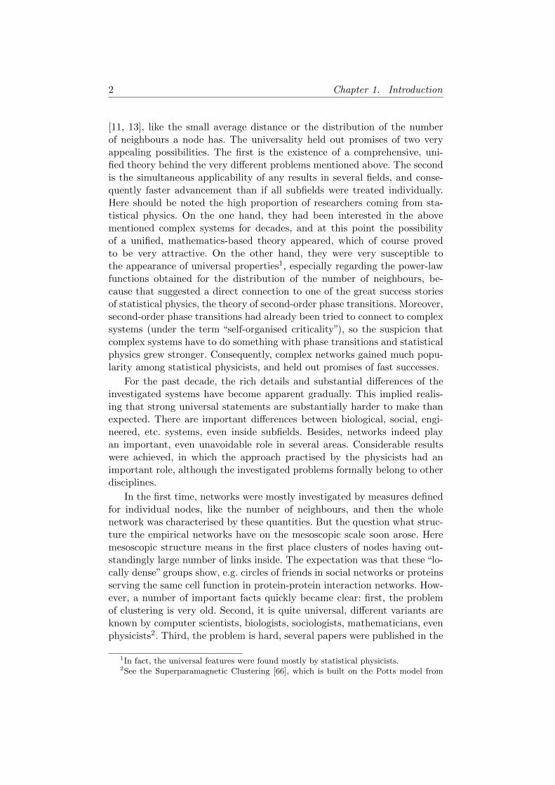
Cells contain several types of networks. There is the metabolic networkof the chemical reactions providing energy and building material for the cell[14], the network of genes regulating each other through protein expression[15], or the network of interacting proteins [171], the cell signallingnetwork [16]. On the level of organs, the human brain is the largestnetwork mentioned in this thesis, built from O(1011) neurons [10], mostprobably giving work for researchers at least for numerous further decades.The relationship of species is represented by a phylogenetic tree, which,due to recently discovered processes like horizontal gene transfer, begun togrow loops. Ecological relationships, like food webs also correspond tonetworks [17]. Diseases can also be associated with each other on the basisof co-occurrence or similar genetic background [18]. Most probably it doesnot require further reasoning to perceive the importance of advancement inthe understanding of the aforementioned examples.
6 Chapter 2. Complex networks in general
Figure 2.1. Biological networks. Top: schematic picture of a food web (figureis from cougarbiology.pbworks.com). Bottom left: schematic tree of life(from tolweb.org). Bottom right: network of interactions of a subset ofgenes from Drosophila melanogaster (from [56]).
Sociology
For a simplified picture, society consists of peoples and links between them[64]. These links serve as an infrastructure for the propagation of news,rumours, information, diseases, habits, or for formation of opinions and col-

2.2. Anatomy of complex network research 7
laborations. As can be seen, several types of connections are possible, andconsequently several different networks can be defined. Although it mightbelong to the previous paragraph, sociological relationships (networks) ofanimal groups can also be studied [19]. Other half-sociological example isthe “social network” constructed for the figures appearing in the ancientGreek mythology [30]. To add a final loosely related example, networks ofwords are quite often investigated [29, 74]. Links can be defined in very dif-ferent ways, like co-occurrence in one sentence, synonyms, or by frequencyof association.
Infrastructure
Most of our infrastructures are networks: roads, railways, air flights connect-ing cities, telecommunication systems, electric power lines, water and sewagesystems are all networks, on which our civilisation depends. A particularlyinteresting line of study in this topic investigates the cascading failure ofpower lines, leading to country-wide blackouts [20].
Computer science
The world of informatics is similarly full of networks as physics with vectorspaces. Function calls within source codes or dependencies between softwarepackages [23] are quite visible even to outsiders. Integrated circuit designalso utilises graphs [24]. The World Wide Web is one of the largest andmost prominent networks, although it also has strong associations beyondcomputer science.
Physics
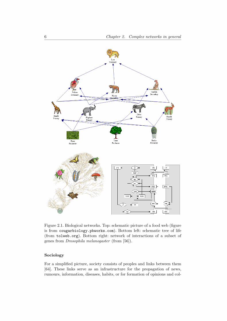
Though physics usually works with vector spaces, graphs do appear a fewtimes. Spin lattices (Ising model) were already mentioned, and a prominentexample of a complex network in physics is a spin glass where the nontrivialway in which the spins are coupled gives rise to a surprisingly complicatedbehaviour. Another example is the network of adjacent local minima of e.g.a cluster of particles interacting by a Lennard-Jones potential [160], whichwas applied to the description of glass transition [25]. The force network ofstatic granular matter was also studied [26], and graphs were applied to thedomain patterns of multiferroic materials [27]. The synchronisation of semi-conductor laser arrays also depend on their connection pattern [28]. Finally,even climate issues, which arise from laws of physics, were investigated bygraphs [32].
8 Chapter 2. Complex networks in general
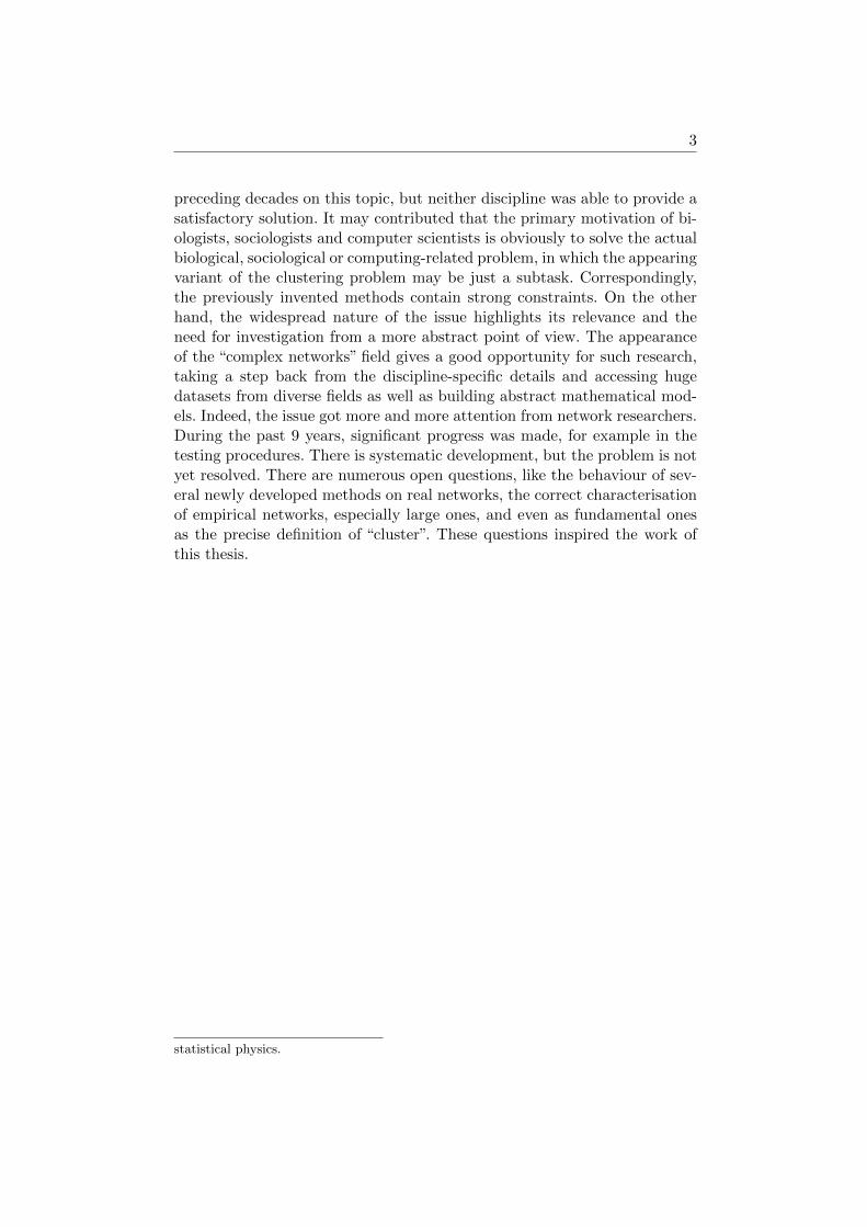
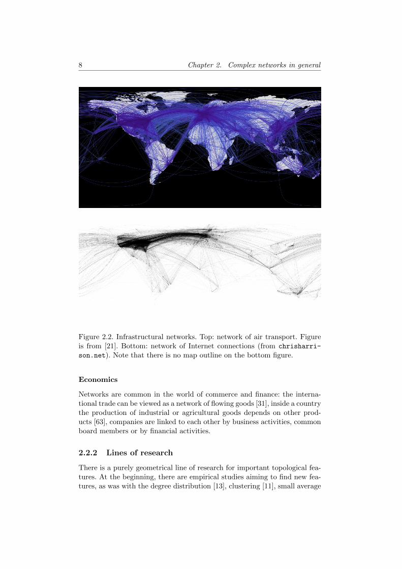
Figure 2.2. Infrastructural networks. Top: network of air transport. Figureis from [21]. Bottom: network of Internet connections (from chrisharri-
son.net). Note that there is no map outline on the bottom figure.
Economics
Networks are common in the world of commerce and finance: the interna-tional trade can be viewed as a network of flowing goods [31], inside a countrythe production of industrial or agricultural goods depends on other prod-ucts [63], companies are linked to each other by business activities, commonboard members or by financial activities.
2.2.2 Lines of research
There is a purely geometrical line of research for important topological fea-tures. At the beginning, there are empirical studies aiming to find new fea-tures, as was with the degree distribution [13], clustering [11], small average

2.2. Anatomy of complex network research 9
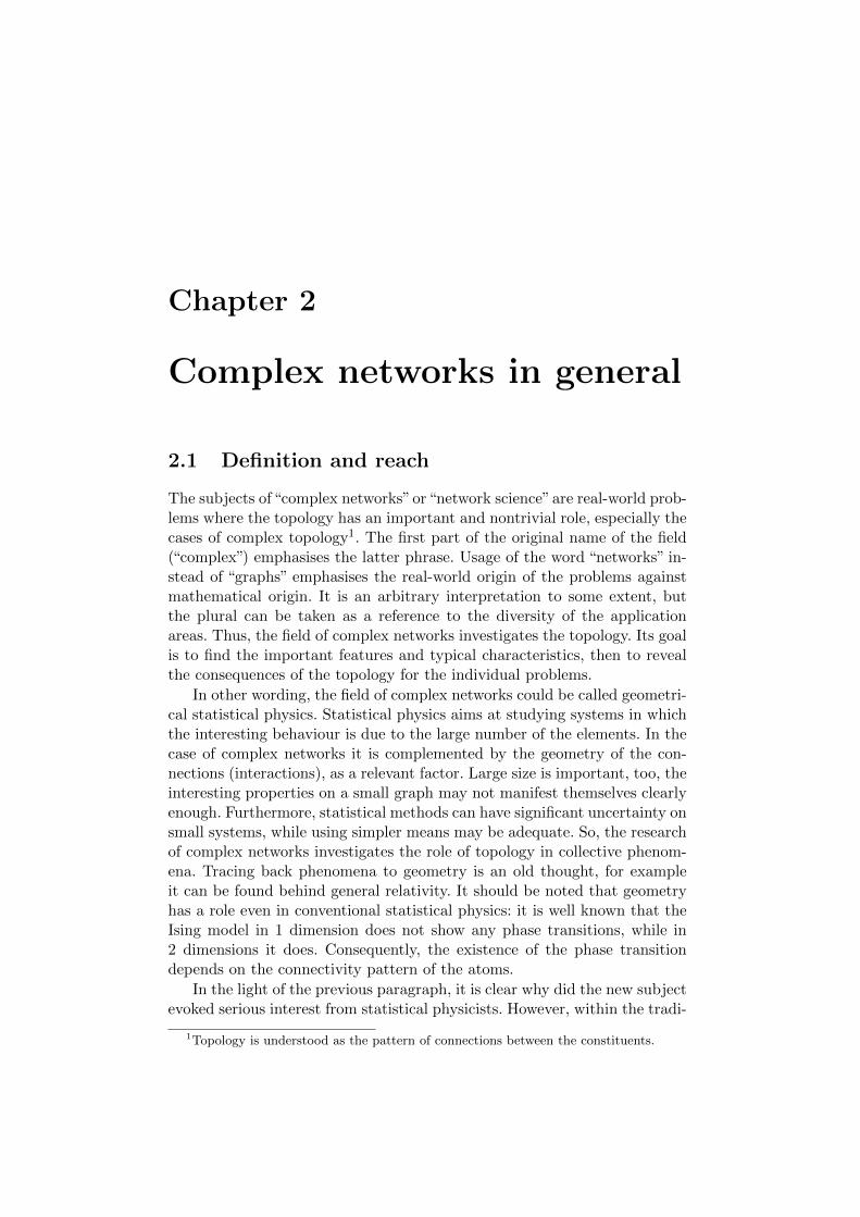
Figure 2.3. A computer-related network – function call network of the seL4microkernel. Figure is from http://ertos.nicta.com.au/.
01
0 01 1
0011
0 01 1
01
0011
010 01 1
01
0 01 10 00 01 11 1
0011
0 00 01 11 1
0 00 01 11 1
01
0011
0011
01
0 01 1
01
01
0 01 1
0011
0 01 1
0011
0011
0 00 01 11 1
Figure 2.4. Network of adjacent local minima of an energy landscape (from[161]).
distance [11, 45], error/attack tolerance [46], [22], searchability [43], fractal-ity [52], motifs [29] or community structure (see the next section for details).After a new feature is found, quantities to describe it are constructed. Thenusually a lot of work goes into developing and analysing models to reproduceand extensively understand the empirical observations.
Furthermore, there are dynamical models which can be placed on graphsand the consequences of different topologies (like lattices of different dimen-sion, small-world graphs, scale-free graphs, clustered graphs) can be investi-gated. Examples are numerous: percolation [33], Ising and Potts models [34],
10 Chapter 2. Complex networks in general
random walk [35], epidemic models [36], synchronisation [150], self-organisedcriticality models [37], models for cascading failures [20], Boolean dynamics[38], chaotic dynamics [39], game theory’s models [40], ecological models [41].This line of research reflects one of the basic questions in network science:how does the topology influence the function of the network?
As can be seen from the above lists, the research on complex networks isstrongly tied to applications, because “important topological feature” has ameaning only if there is some real-world context in which it has consequences.
2.3 Important concepts and results
2.3.1 General results
It follows from the nature of complex networks research that it tries to finduniversal features which appear over a wide range of fields, independentlyfrom much of the discipline-dependent details. The statistical physics back-ground of several researchers makes this ambition even more pronounced.
Even the first findings about complex networks had a very strong uni-versal nature. Three features were identified in the first years:
Small average distance the average distance between a pair of nodes inmost empirical networks were found to be much smaller than the net-work size (“small world” phenomenon) [42, 10, 43]. E.g. for a networkof coauthorships in biology-related articles, the average distance wasslightly less than 5, while the network contained more than one and ahalf million of nodes. Typically, the average distance was below 10 fornetworks ranging from hundred to millions of nodes, and was alwaysless than 20. Further analysis revealed that networks can easily haveaverage distances growing logarithmically (or even slower [45]) withthe network size. On regular graphs, even a small amount of shortcutlinks is enough to produce the effect [11].
Clustering the so-called clustering coefficient denotes the number of tri-angles in a specific node’s neighbourhood, divided by the number ofpossible triangles. This quantity measures a kind of correlation be-tween the links. For several real cases the average clustering coefficientturned out to be quite high, orders of magnitude higher than for asimilarly-sized random graph2 [11, 42, 10, 43]. This suggests that linksare generated locally in many types of networks.
Broad degree distribution the distribution of the number of neighboursof the nodes, the degree, was found to strongly deviate from those ofthe (Erdos-Renyi) random graphs in most cases [13, 42, 10, 43]. The
2More specifically, “random graph” refers to the Erdos-Renyi stochastic graph model,in which all node pairs are connected by a constant probability. [12]

2.3. Important concepts and results 11
degree distributions were stretched such that “hub” nodes with veryhigh degrees (like the square root of the network size) were present.In fact, the degree distributions were approximated in most cases bya power law, with exponents between −2 and −3, although there arewarnings that these distributions may not be power laws [50, 51]. Theslowly decaying degree distribution has a profound effect on most geo-metric and dynamic features. A notable exception is the class of socialnetworks, for straightforward reasons – no one can have thousands offriends.
These findings triggered the definition of new types of graph models,which provided new topologies for existing dynamical models. Furthermore,building on the above findings, other results soon appeared. Resilience againstrandom or targeted node removal (modelling failures/attacks) turned out todepend heavily on the degree distribution: graphs with power-law degree dis-tributions are very robust to random node removal and sensitive to targetednode removal [46].
Other interesting facts were found in connection with epidemic spreadingmodels. Conventional wisdom stated that a disease’s fitness should pass acertain threshold in order to infect a macroscopic portion of the population.It turned out that on graphs with broad degree distributions3 the thresholdvanishes4, meaning that arbitrarily incapable diseases can make an epidemic[47]. This applies both to biological and computer viruses. For the latter case,viruses persisted in the Internet several months after the antivirus softwaresgot their updates [47]. Although the absence of the threshold may not holdin all real-life cases, it clearly signs the effect of the topology.
Sticking to the degrees, it was observed from the correlations of degreesof neighbouring nodes that there is a so-called rich-club phenomenon in ascientific coauthorship network: nodes with large degrees are disproportion-ally well connected to other large-degree nodes [48]. It was hypothesised thatother social networks may also show this effect.
Single-node and two-node characteristics were not the only statisticalfeatures considered. The occurrence of different small connection patterns,sized of just a few nodes, was compared to occurrence frequencies in randomgraphs, for various networks [29]. It turned out that real-world networkshad some connection patterns overrepresented (these were called motifs),and some other ones underrepresented (antimotifs). Very interestingly, themotif-antimotif profiles were classifiable into a few family, networks of similartype appearing in the same family. E.g. the represented language networks(English, French, Spanish, Japanese, and a language model network) allhad the same motifs and antimotifs. For some cases, especially in biologicalnetworks, motifs can be associated with specific functions [49].
3To be precise, for which the variance of the degree diverges.4In the infinite network size limit.
12 Chapter 2. Complex networks in general
The term “scale-free network” originated from the finding that severalempirical networks have a broad degree distribution, strongly resembling toa power law function, at least on an interval. Power law functions do not havea characteristic scale, hence the name. However, the “scale-free” status wasquestioned from two directions. First, the initially assigned power laws of theempirical degree distributions were disputed in a number of cases [50, 51].Second, and this is a much more interesting direction, it was far from clearwhether the investigated networks show any kind of self-similarity underrenormalisation or not. The generally found logarithmic average distancesuggested a negative answer. Instead, after properly defining a renormali-sation method for networks, it turned out that several empirical networksare fractals5 [52]; in the sense that the number of boxes needed to coverthem grows as a power of the box diameter. On the other side, the mostwidespread network models, some of them having a true power law degreedistribution, turned out to not being fractals. Later, models reproducingfractality were invented [53, 54].
Finally, it should be noted that much work have been devoted to networksthat are more complicated than just set of nodes and edges: nodes canhave properties (like tags [55]), edges can be directed or can carry weights(like bandwidth) [44, 43]. Some networks have a special structure calledbipartiteness: nodes can be coloured by two colours such that each edgeconnects nodes of different colours [43].
2.3.2 Some application results from complex networks ingeneral
Drosophila segmentation
The embryonic pattern formation of the fruit fly Drosophila melanogasterwas modelled by gene interactions networks [56]. As an insect, the body ofDrosophila is segmented, and the cell types in the segments are determinedby a network of genes. In the model, neighbouring cells’ networks were cou-pled to each other. The interactions were known from experiments. A prop-erly chosen Boolean dynamics modelled these interactions, the steady statescorresponding to observable patterns on the flies. It turned out that only 6steady states exists, 3 of them were experimentally observed earlier, and theothers requiring very improbable conditions. It was also discovered that thesteady state corresponding to the normal fly is very robust to biologicallyrelevant perturbations of the initial state.
5Fractals are geometrical objects being similar to themselves after magnification. Thisfeature is closely tied to the appearance of power law functions.
2.3. Important concepts and results 13
Industrial development
The possibilities for developing new industrial products from existing onescan be modelled as moving on a graph of products. A reconstruction ofthe product proximity network from observed production data was done by[63]. The reconstructed network looked very different from the ones impliedby the current economical models, showing a core-periphery structure withmodular units. The modular structure corresponds well to previous classi-fication of products (e.g. garments, animal agriculture or electronics). Thestrong links tend to be in the core, and in a few peripheral modules. It wasalso confirmed that countries typically develop new products which are closeto already existing ones. These findings imply that countries with differentcurrent product profile are in different positions for future development, e.g.countries having products on the periphery possessing much more restricteddevelopment possibilities than countries being active in the core or in amodule. Indeed, different regions of the world occupy different characteris-tic regions in the product proximity network, the richness of the countriesstrongly correlating with the centrality of their product in the network.
Synthetic rescues in metabolic networks
Deletion of a metabolism-regulating gene damages the metabolic pathways,reducing the productivity of the cell, e.g. its growth rate, in some cases toa non-viable level (essential genes). However, lethal gene deletions may beturned to non-lethal by the deletion of additional genes [57]. The mecha-nism is the following. After a gene deletion, the cell tries to adapt by aminimal amount of metabolic flux rearrangement, leading to a far-from-optimal state. Meanwhile, a global rearrangement of the fluxes can result inmuch more optimal state, comparable to the one of the unharmed cell. Theglobal flux rearrangement can be triggered by further gene deletions. Theidea was applied to organisms as Escherichia Coli, Helicobacter pylori andSaccharomyces cerevisiae, revealing dozens of potential rescue combinationsfor each. Although the approach is based on computations applied to knownmetabolic systems, reanalysing previous experiments showed evidence thatthe method works in real life. It is interesting to note that inspiration camepartly from a proposed method to stop cascading failures on electric net-works.A similar approach was also applied in connection with ecological networks[58].
Confirmation of the weak ties hypothesis
In sociology, Granovetter hypothesised that acquaintance networks containclusters of people densely interconnected with strong links, while the clustersare hold together by weak links. In spite of the fact that this “Strength of
14 Chapter 2. Complex networks in general
Weak Ties” hypothesis became one of the most influential ones in sociology,empirical evidence had not been available beyond small-scale surveys, untilrecently. In the last years, a few databases of mobile phone providers becameaccessible, providing insight into the communication habits of macroscopicparts of entire societies. Using the frequencies of mobile phone calls as linkstrengths, it was possible to obtain an approximation of the underlying so-cial network [59]. It turned out that the overlap between a link’s two ends’neighbours is monotonically increasing with the link strength (except for thestrongest 5% of the links), verifying the weak ties hypothesis on a samplecontaining millions of people, and – not less importantly – applying an ob-jective link strength measure. The weak ties hypothesis is just one example,other sociological hypotheses were also tested or even formed by the analysisof large empirical networks [151].
2.4 Tools
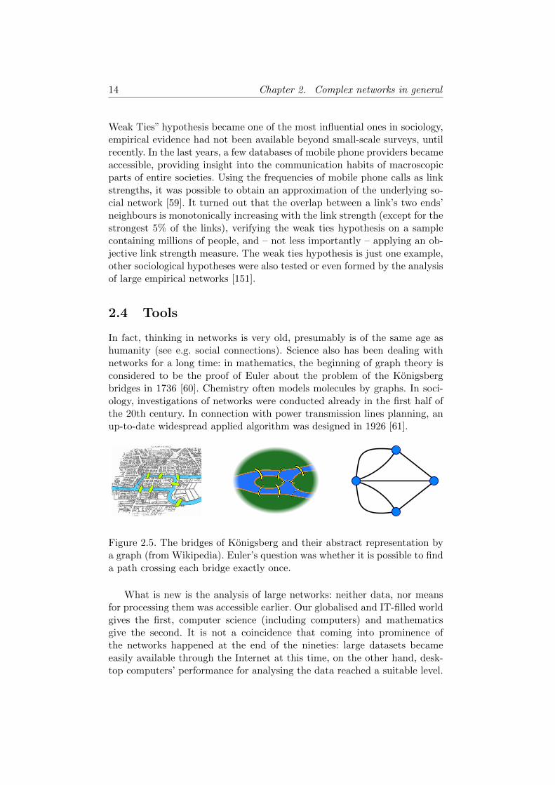
In fact, thinking in networks is very old, presumably is of the same age ashumanity (see e.g. social connections). Science also has been dealing withnetworks for a long time: in mathematics, the beginning of graph theory isconsidered to be the proof of Euler about the problem of the Konigsbergbridges in 1736 [60]. Chemistry often models molecules by graphs. In soci-ology, investigations of networks were conducted already in the first half ofthe 20th century. In connection with power transmission lines planning, anup-to-date widespread applied algorithm was designed in 1926 [61].
Figure 2.5. The bridges of Konigsberg and their abstract representation bya graph (from Wikipedia). Euler’s question was whether it is possible to finda path crossing each bridge exactly once.
What is new is the analysis of large networks: neither data, nor meansfor processing them was accessible earlier. Our globalised and IT-filled worldgives the first, computer science (including computers) and mathematicsgive the second. It is not a coincidence that coming into prominence ofthe networks happened at the end of the nineties: large datasets becameeasily available through the Internet at this time, on the other hand, desk-top computers’ performance for analysing the data reached a suitable level.
2.4. Tools 15
Accessible data kept expanding: in biology, high throughput methods, insociology, the online activities and mobile phones are producing new dataat such rates that processing them is possible exclusively by computers.
Importance of the new data is high. The number one example is soci-ology, for which totally new possibilities opened up, because earlier it hadonly small-scale surveys, often carrying very subjective content. Thereforechecking hypotheses and making empirical observations was very stronglyrestricted. Compared to this, today it is possible, using mobile phone calls,to reconstruct an approximate acquaintance network of millions of people,based on objectively measured data [151, 59, 62].
Beyond the large number of constituents, these networks have anotherimportant feature: they do not possess an easily understandable structure,contrary e.g. to the lattices. Usually they are generated by very complexprocesses, so the easiest way of modelling them is to use stochastic models.For that reason, they offer a large scope for the application of probabilitytheory and statistical methods. Due to the large number of constituents andthe stochastic character, application of the methods of statistical physics,like mean-field theory, is an obvious idea. For the same reason, applicationof computer simulations also arises naturally, e.g. for investigation of models.
Chapter 3
Introduction to communitydetection on complexnetworks
A natural question about a network is whether it has dense regions, denserthan the average. These regions, if present, correspond to mesoscale struc-tures in the network – larger than the individual nodes, but smaller than thewhole network. Common sense suggests that such subgraphs should carryrelevant information, like people having a common interest in a social net-work, or biochemicals belonging to the same pathway in metabolic networks.
It is not surprising that the question of dense subgraphs appeared incomplex networks research; in fact, currently it is the one of the most activelyinvestigated topics [65], under the term “community detection”.
3.1 Historical overview
The clustering of objects is a much older problem than the activity aboutcommunity detection among network researchers. Classification can be tracedback to Aristotle. In biology, the modern systematic grouping of creatureswas introduced by Carolus Linnaeus in the eighteenth century, and clusteringproblems still occur in our days, e.g. in DNA sequence analysis. Sociologistshave talked about cliques, clans, LS-sets, etc. all being some quantitativedefinition for “cohesive subgroups”, for decades [64]. The same is true forblockmodelling, i.e. decomposing a (social) network into classes of nodeswith common properties [65]. In computer science, graph partitioning hasbeen applied for load balancing in parallel computing, or in integrated cir-cuit design, also for decades [65]. Even statistical physicists built clusteringmethods previously, e.g. the famous Superparamagnetic Clustering method,which is based on the Potts model [66].
In connection with networks, the concept of clusters appeared first in
3.1. Historical overview 17
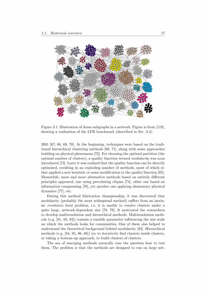
Figure 3.1. Illustration of dense subgraphs in a network. Figure is from [119],showing a realisation of the LFR benchmark (described in Sec. 3.4).
2001 [67, 68, 69, 70]. At the beginning, techniques were based on the tradi-tional hierarchical clustering methods [69, 71], along with some approachesbuilding on physical phenomena [72]. For choosing the optimal partition (theoptimal number of clusters), a quality function termed modularity was soonintroduced [73]. Later it was realised that the quality function can be directlyoptimised, resulting in an exploding number of methods, most of which ei-ther applied a new heuristic or some modification to the quality function [65].Meanwhile, more and more alternative methods based on entirely differentprinciples appeared, one using percolating cliques [74], other one based oninformation compressing [76], yet another one applying elementary physicaldynamics [77], etc.
During this method fabrication championship, it was discovered thatmodularity (probably the most widespread method) suffers from an intrin-sic resolution limit problem, i.e. it is unable to resolve clusters under aquite large, network-dependent size [78, 79]. It motivated the researchersto develop multiresolution and hierarchical methods. Multiresolution meth-ods (e.g. [81, 82, 83]) contain a tunable parameter influencing the size scaleon which the methods looks for communities. One of them also helped tounderstand the theoretical background behind modularity [83]. Hierarchicalmethods (e.g. [84, 85, 86, 88]) try to iteratively find clusters inside clusters,or taking a bottom-up approach, to build clusters of clusters.
The sea of emerging methods naturally rose the question how to testthem. The problem is that the methods are designed to run on large net-
18 Chapter 3. Introduction to community detection
works, and no large empirical network with known cluster structure wasknown (which still holds). Therefore, testing in the first times was done ona few small empirical networks, with some a priori information about sus-pected communities. Later, artificial benchmarks appeared and graduallyimproved.
Another critical question is to decide how meaningful the results are. Itwas realised soon, that modularity (which measures the quality of a parti-tion) takes quite high values on random graphs without cluster structurebesides statistical fluctuations [89]. Later it was discovered that modularity– and other methods too – has several local optima, having similar qual-ity values but corresponding to rather different clusterings [90, 91, 92]. Apromising way for choosing the correct clusters is checking the statisticalsignificance of the found clusters, for which methods have begun to appearrecently [93, 94].
Besides the theoretical considerations, more practical aspects were ad-dressed, too. It was proven that optimising modularity is an NP-completeproblem [95], and there is no reason to assume that for other measures thesituation is substantially better. This makes clear the importance of devel-oping good heuristics. A significant amount of work was put in the reductionof required time. Some algorithms required O(N3) running time (N is thenumber of nodes), which is intractable for large – say, N ≥ 104 – networks1.Now more algorithms with low time requirement are available, surprisinglywith very good test results [96]. E.g. a network of 5 million of nodes and 11million of edges was processed in 2 days by a very precise algorithm, and inless than 5 minutes by 2 other ones [91].
3.2 Relation to statistical physics
The basic models for networks, although differ in their global structure, havelocally homogeneous edge densities, up to statistical fluctuations. This is asymmetry, although in a statistical sense, similar to the (statistically) homo-geneous density of a gas. It is very natural to ask whether this symmetry doeshold for real-world networks, or local condensations of edges are observable.Such type of questions immediately raise the interest of physicists. On theother hand, there are important differences to traditional physical systems:experiments are rarely possible (think e.g. on social networks), even data onthe evolution of systems is not always accessible, so usually only individualinstances of the networks are observable. Furthermore, in traditional statis-tical physics, appearance and disappearance of a symmetry can be usuallytuned by a single parameter, like temperature – it is not evident whether
1The networks of interest are usually sparse, the number of links being proportional tothe number of nodes. Therefore, dependency of the running time on the number of linkscan be conveniently expressed by the number of nodes.
3.2. Relation to statistical physics 19
such a parameter can be found for the inhomogeneity of the edge density innetworks.Despite the complications, ideas from statistical physics were borrowed assoon as the issue emerged. Researchers began to talk about hierarchicallyembedded structures, which are of central importance in spin glass theory.Furthermore, the so-called multiresolution methods also lean on a pictureoriginating from statistical physics. They sequentially look for clusters whilechanging a resolution parameter, resulting in cluster structures having differ-ent typical cluster sizes. It is assumed that for a network with a real clusterstructure, the found clusters will not change continuously while tuning ofthe resolution parameter, instead the real clusters will be found again andagain over an extended parameter range. This is in contrast to the pictureof second-order phase transitions, where clusters exist on all scales, neitherscale being more dominant than the others – a symmetry, expected to bebroken for real networks.
If there are locally dense subgraphs in a graph, they should manifestthemselves in various physical processes which take place on the graph. Ob-serving the inhomogeneities in such processes opens a way to the detectionof clusters. This is what a physicist tend to think when presented with theproblem of community detection. The presence of several elementary units(network nodes) and the stochastic nature of the interconnections directsnaturally to statistical physics, which already had previous experiences withsome kinds of clusters.
For example, it is expected that a diffusion on a clustered graph will re-flect the cluster structure. Diffusion can be modelled in mathematical termsby random walks. A random walker should spend long times inside the clus-ters, so identification of sets of nodes from which the random walker does notescape easily provides our target. This picture attracted recurring attention[97, 98, 83], leading to remarkable methods.
Besides diffusion, one can expect that a Potts model defined on the graphin question should also reflect the dense clusters. The problem is that themost natural configuration, the ground state at zero-temperature, is trivial,consequently does not provide any information about the clusters. The firstidea to circumvent this problem was to use finite temperature, this lead tothe Superparamagnetic Clustering method [66] in 1996, a few years earlierthan networks came into fashion. Some years later, it was proposed to avoidthe trivial solution by introducing antiferromagnetic couplings (“negativelinks”), transforming the Potts Hamiltonian to a frustrated spin glass-typeone. Several different definitions for the new couplings are known (see e.g.[81], [119]). As a third approach, a simple dynamics equivalent to findingthe zero-temperature higher local minima of the original Potts model wasalso proposed [77], [92].
Beyond the Potts model, statistical physics also knows clusters from per-colation problems. Correspondingly, percolation-based community detection
20 Chapter 3. Introduction to community detection
methods appeared [74].
3.3 Definition of the problem
Probably the most important problem of the community detection subfieldis the lack of a generally accepted precise definition of communities. Defin-ing the term “cluster” in a mathematically precise way is a nontrivial task.So nontrivial that no widely-agreed definition exists. The most precise termcurrently is “nodes having more edges among themselves than to the restof the graph”. Clearly, it is not enough to unambiguously build a detectionmethod. On the other side, when hearing about clusters, everyone immedi-ately has a conception about it. This stress between the naturality of theintuitive picture and the difficulty of the precise definition is one of the majormotivation factors behind the research.
A cluster can have different meanings for different fields. E.g. in sociology,a community of people is expected to have very small average distances, anda lot of triangles. In metabolic networks, a pathway can be a much moreelongated subgraph. In computer science applications, any subgraph whichis well separated and not very small might be a good cluster. Furthermore,clusters may be defined on the basis of some activity of the nodes in reallife, which is not necessarily reflected in the topology of the network [75]. So,“cluster“ usually has more or less different meanings in different contexts,and correspondingly, different detection methods are required.
In spite of the above difficulties, it seems that behind the huge amountof papers labelled as community detection, there is a certain type of objectsfor which the researchers look for. It may be called locally dense subgraph.What is important not the exact term, but the properties which it is aimedto reflect: first, our objects are determined solely by the graph topology, notby functions performed by the network. Second, clusters are defined on alocal basis – they should be recognised considering only the cluster and itslocal neighbourhood, without taking into account the whole graph or distantregions of it. Third, nothing is imposed on the clusters regarding the sizes ornumber of the clusters, allowing e.g. broad size distributions. Finally, clustersare not restricted to form a partition, i.e. nodes may belong to zero or tomultiple clusters – such a set of clusters is called a cover. Consequently, theproblem of community detection is more general and also more difficult thanfinding a partition or finding clusters with the aim of some constraints, likea fixed number of clusters or other information originating from a sourceexternal to the graph topology. As no specific features are supposed forthe clusters, it is hard to imagine a more general version of the clusteringproblem. The lack of formal definition, mentioned in the first paragraph ofthis section, partly stems from this generality, but just partly: setting e.g.the expected cluster sizes does not solve the question of definition.
3.4. Difficulties 21
3.4 Difficulties
Most current methods hypothesise that the community structure of a net-work corresponds to a partition, i.e. all nodes belong exactly to one com-munity. However, life can be more complicated. For example, there can be ahierarchy of communities: large clusters may contain smaller clusters, whichcan contain even smaller cluster, . . . Although this is a familiar situationfor the ones with spin glass theory background, it is even more familiar fromeveryday life: from the organisation of institutions and firms, or from bi-ology (cell-tissue-organ-organism). Beyond the discrete levels of hierarchy,networks may have a cluster structure which changes more or less continu-ously with the scale of investigation, like zooming in on a map reveals moreand more details.
Furthermore, in many networks it is natural to assume that nodes canbelong to multiple communities. E.g. in a social network, one can have a fam-ily, friends, colleagues, sports team, etc. – or in unfortunate cases, he/shecan live lonely, without any close community, which translates that nodesnot necessarily belong to communities. Generalising the overlapping com-munities, nodes may belong to different communities to a different degree,requiring fuzzy or ”soft“ memberships from the real interval [0.1].
Beyond problems with the communities, additional features of the net-work, like weighted or directed edges, or bipartiteness also raise further com-plications.
A different kind of complication comes from a much more practical as-pect. The networks to be analysed are usually large (current record is atleast 6.5 · 108 nodes [108]). Sizes of this magnitude require the applied al-gorithms to be fast, being essentially linear in CPU time as function of thesize of the network.
Beyond the question of definition of communities, the other very impor-tant problem with community detection is how to decide whether a proposedmethod is good or bad. There are two approaches for testing methods: ei-ther on empirical networks or on artificial ones. Empirical networks withknown community structure tend to be small (< 150 nodes), because largernetworks are very hard to oversee and annotate the clusters by eye. Evenfor small enough networks, known cluster structure is usually deduced fromsome source outside the network topology, questioning the appropriatenessof comparing them to topology-deduced communities. For quite a long, mostmethods were usually examined only on a few empirical networks, like theZachary karate club (34 nodes) [101], which was split into two during theobservation, due to a dispute. The other frequently occurring test cases are asocial network of bottlenose dolphins (62 nodes), and a network of Americanfootball teams (115) nodes. Naturally, one does not expect to gain a com-prehensive picture about a method’s capabilities, based on such a testing.
The other possibility is to use artificial graphs with built-in community
22 Chapter 3. Introduction to community detection
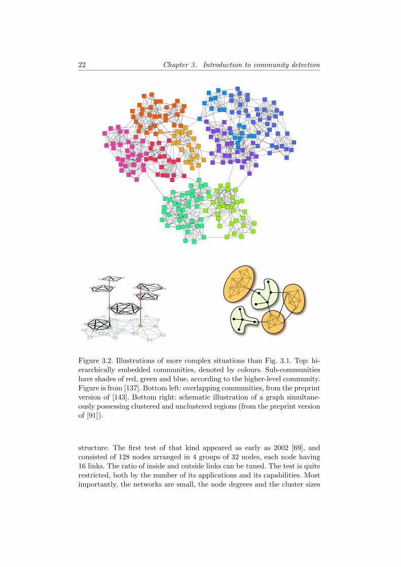
Figure 3.2. Illustrations of more complex situations than Fig. 3.1. Top: hi-erarchically embedded communities, denoted by colours. Sub-communitieshave shades of red, green and blue, according to the higher-level community.Figure is from [137]. Bottom left: overlapping communities, from the preprintversion of [143]. Bottom right: schematic illustration of a graph simultane-ously possessing clustered and unclustered regions (from the preprint versionof [91]).
structure. The first test of that kind appeared as early as 2002 [69], andconsisted of 128 nodes arranged in 4 groups of 32 nodes, each node having16 links. The ratio of inside and outside links can be tuned. The test is quiterestricted, both by the number of its applications and its capabilities. Mostimportantly, the networks are small, the node degrees and the cluster sizes
3.4. Difficulties 23
are homogeneous, although both are known to have broad distributions inempirical cases.
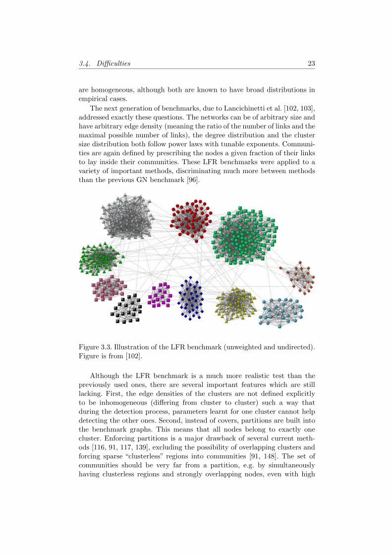
The next generation of benchmarks, due to Lancichinetti et al. [102, 103],addressed exactly these questions. The networks can be of arbitrary size andhave arbitrary edge density (meaning the ratio of the number of links and themaximal possible number of links), the degree distribution and the clustersize distribution both follow power laws with tunable exponents. Communi-ties are again defined by prescribing the nodes a given fraction of their linksto lay inside their communities. These LFR benchmarks were applied to avariety of important methods, discriminating much more between methodsthan the previous GN benchmark [96].
Figure 3.3. Illustration of the LFR benchmark (unweighted and undirected).Figure is from [102].
Although the LFR benchmark is a much more realistic test than thepreviously used ones, there are several important features which are stilllacking. First, the edge densities of the clusters are not defined explicitlyto be inhomogeneous (differing from cluster to cluster) such a way thatduring the detection process, parameters learnt for one cluster cannot helpdetecting the other ones. Second, instead of covers, partitions are built intothe benchmark graphs. This means that all nodes belong to exactly onecluster. Enforcing partitions is a major drawback of several current meth-ods [116, 91, 117, 139], excluding the possibility of overlapping clusters andforcing sparse “clusterless” regions into communities [91, 148]. The set ofcommunities should be very far from a partition, e.g. by simultaneouslyhaving clusterless regions and strongly overlapping nodes, even with high
24 Chapter 3. Introduction to community detection
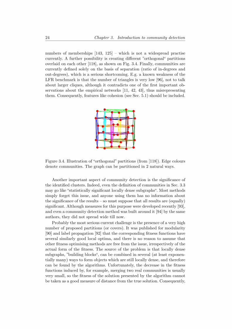
numbers of memberships [143, 125] – which is not a widespread practisecurrently. A further possibility is creating different ”orthogonal“ partitionsoverlaid on each other [118], as shown on Fig. 3.4. Finally, communities arecurrently defined solely on the basis of separation (ratio of in-degrees andout-degrees), which is a serious shortcoming. E.g. a known weakness of theLFR benchmark is that the number of triangles is very low [96], not to talkabout larger cliques, although it contradicts one of the first important ob-servations about the empirical networks [11, 42, 43], thus misrepresentingthem. Consequently, features like cohesion (see Sec. 5.1) should be included.
Figure 3.4. Illustration of “orthogonal” partitions (from [118]). Edge coloursdenote communities. The graph can be partitioned in 2 natural ways.
Another important aspect of community detection is the significance ofthe identified clusters. Indeed, even the definition of communities in Sec. 3.3may go like “statistically significant locally dense subgraphs“. Most methodssimply forget this issue, and anyone using them has no information aboutthe significance of the results – so must suppose that all results are (equally)significant. Although measures for this purpose were developed recently [93],and even a community detection method was built around it [94] by the sameauthors, they did not spread wide till now.
Probably the most serious current challenge is the presence of a very highnumber of proposed partitions (or covers). It was published for modularity[90] and label propagation [92] that the corresponding fitness functions haveseveral similarly good local optima, and there is no reason to assume thatother fitness optimising methods are free from the issue, irrespectively of theactual form of the fitness. The source of the problem is that locally densesubgraphs, ”building blocks“, can be combined in several (at least exponen-tially many) ways to form objects which are still locally dense, and thereforecan be found by the algorithms. Unfortunately, the decrease in the fitnessfunctions induced by, for example, merging two real communities is usuallyvery small, so the fitness of the solution presented by the algorithm cannotbe taken as a good measure of distance from the true solution. Consequently,

3.5. Other fields’ methods 25
algorithms are expected to end up in one of the several suboptimal clusterstructures, even if being run several times (then most probably returningseveral different suboptimal partitions).
3.5 Other fields’ methods
Various clustering methods had been developed before the term ”communitydetection“ was born. In contrast with the methods discussed in the nextsection, they usually require the number of clusters as input, which is amajor drawback.
Probably the most well known is the k-means clustering [104], whichrequires a metric space. The idea is to find k clusters such that the variancesof the clusters (sums of squared distances from centres) are minimal. k isan input. The common solving algorithm goes as follows: initially k clustercentres are chosen somehow (e.g. randomly), and nodes are assigned to thenearest centre. Then the centre of each cluster is recalculated (this timeas the centre of mass), and nodes are reassigned. The steps are iterateduntil convergence. The method implicitly assumes sphere-like, similarly sizedclusters.
Another method is the Principal Component Analysis (PCA) [105]. Infact, it is not strictly a clustering method, instead a dimension reductiontechnique. Given a similarity matrix (e.g. a correlation matrix), PCA projectsthe matrix to a k dimensional subspace which basis vectors have the largestvariances from all possible k dimensional subspaces, k being an input param-eter. This way, the maximal variability possible in k dimensions is preserved.If there are clusters in the data, they are expected to show up in the pro-jected data, and can be directly observed if k = 2 or 3. PCA can be done byeigenvalue decomposition. It is known that PCA and k-means clustering arerelated: the principal components give the optimal solution of the k-meansproblem.
A different approach is the family of hierarchical clusterings [106]. Givena similarity matrix, the hierarchical clustering successively merges elementswith the highest similarity, until the whole dataset belongs to a single cluster.The merging process can be described by a tree, called dendrogram, whichleaves are the original objects, and the internal branching points correspondto clusters. To obtain a cluster structure, the dendrogram should be cut atsome point, the choice depending on the user. For example. prescribing thenumber of cluster defines a cutting point.
An alternative form of the hierarchical clustering is the Maximal Span-ning Tree [61], which is a graph built from the objects and their similarities,such that the resulting graph has no loops (“tree”), reaches all nodes (“span-ning”), and has maximal sum of similarities from all possible spanning trees(“maximal”). Branches in the MST are expected to correspond to clusters.
26 Chapter 3. Introduction to community detection
It can be shown that the MST gives the same clusters as the hierarchicalclustering of the so-called single linkage type, where similarity of two clustersis defined as the similarity of their most similar members.
Other methods also exist, applying e.g. neural networks or support vectormachines [107].
3.6 Overview of the current methods
Here a representative but not exhaustive list is presented – important meth-ods from both theoretical and practical point of views are mentioned.
3.6.1 Random walk-based methods
Random walk is the mathematical model for diffusion, which is one of thefirst phenomena showing the presence of clusters that a physicist wouldname. Correspondingly, several attempts were made to attack the clusteringproblem from this side. Getting information about clusters by using randomwalks belongs to the class of nontrivial problems for which it can be saidthat we know how to solve it [83], [98].
In the following, the most important attempts will be described.
Eriksen et al’s method
Consider the adjacency matrix (A) of a graph, which ij element is 1 if nodesi and j are connected and 0 otherwise. It is easy to see that to describe arandom walk, the required transfer matrix T is obtained by normalising theAij entry of the adjacency matrix by the degree of node j,
Tij = Aij/kj (3.1)
This matrix has an eigenvalue 1 corresponding to the stationary state2, inwhich the random walker density on each node is proportional to its degree.One suspects that if the investigated graph has clusters in which the randomwalker can be trapped, slowly decaying modes (i.e. eigenvalues close to 1)appear. In 2003, Eriksen et al [97] used the eigenvalues and eigenvectorsof T to show that there are indeed slowly decaying eigenmodes for theInternet graph, associated with different countries. It was further argued thatnodes belonging to the same cluster behave similarly in different eigenmodes,i.e. the ratio of eigenvector components corresponding to one node is thesame within a module. Consequently, plotting two eigenvectors’ componentsshould result in straight lines with different slopes, corresponding to differentclusters.
2The multiplicity of this eigenvalue equals to the number of connected components inthe graph.
3.6. Overview of the current methods 27
Although being usable only on a very easily recognisable communitystructure, the method demonstrated that diffusion indeed contains informa-tion about the clusters.
Infomap
After some further attempts involving random walks [109, 110, 111], a reallyusable method came in 2008 by Rosvall and Bergstrom [98]. It tries to com-press the description length of a random walk, by using clusters. The idea isthat a node ID should be unique only for the cluster of that node, thereforeintroducing clusters makes it possible to use short node IDs. As the clustersalso have IDs, too much clusters or large cluster-crossing probabilities in-crease the description length. The best partition is a trade-off between toomany small clusters (short node IDs but long & frequently used cluster IDs)and too few large clusters (short and infrequent cluster IDs in the randomwalk path, but long node IDs). A clever effective heuristic was also pre-sented, which allows the analysis of graphs of millions of nodes. The methodperformed rather well in the (state-of-the-art) LFR benchmark, actuallybeating all of its rivals. Till now, only one very recent method [94] was ableto reach its performance on the LFR test. Recently, Infomap was extendedto handle hierarchically structured communities [86] and overlapping nodes[87], as well as to overcome its susceptibility to overpartitioning in certainsituations [99].
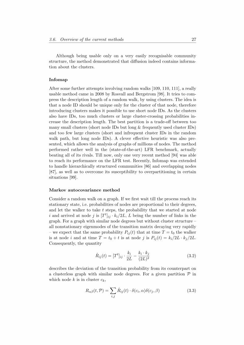
Markov autocovariance method
Consider a random walk on a graph. If we first wait till the process reach itsstationary state, i.e. probabilities of nodes are proportional to their degrees,and let the walker to take t steps, the probability that we started at nodei and arrived at node j is [T t]ij · ki/2L, L being the number of links in thegraph. For a graph with similar node degrees but without cluster structure –all nonstationary eigenmodes of the transition matrix decaying very rapidly– we expect that the same probability Pij(t) that at time T = t0 the walkeris at node i and at time T = t0 + t is at node j is Pij(t) = ki/2L · kj/2L.Consequently, the quantity
Rij(t) = [T t]ij ·ki2L− ki · kj
(2L)2(3.2)
describes the deviation of the transition probability from its counterpart ona clusterless graph with similar node degrees. For a given partition P inwhich node k is in cluster ck,
Rαβ(t,P) =∑i,j
Rij(t) · δ(ci, α)δ(cj , β) (3.3)
28 Chapter 3. Introduction to community detection
measures the accumulated deviations for starting in cluster α and endingin β. The trace of this matrix can be used to indicate the quality of apartition. Consequently, communities can be obtained by maximising thetrace of R(t,P) over P by a suitable heuristic, as proposed by Delvenne etal. [83]. The name of the method follows from the fact that R(t,P) givesthe autocovariance matrix of the random walk observed at the cluster level.
The method has one free parameter, the timescale at which the randomwalk is evaluated. Both intuition and actual results tell us that small tgives very small clusters and large t gives large clusters. The original work[83] proposed to search for partitions that are optimal over a large rangeof timescales; the most robust ones corresponding to the most significantpartitions of the network on different scales. This way, the time parameteris effectively handled as a resolution parameter for the cluster size. This wasmarketed as a strong point of the method, in contrast to modularity (see afew paragraphs later) with its resolution limit.
Interestingly, several formerly known measures for clustering turned outto be some limiting cases of this method. The largest surprise was thatmodularity is the t = 1 special case of trace R(P). The surprise was dueto the fact that modularity was proposed in a static framework withoutany reference to random walks, and classified as a special type of spin glassproblems. The basic multiresolution variant of modularity [81] turned out tobe the linearised t < 1 version of the Markov autocovariance method. Theother proposed multiresolution variant for modularity [82] is also related ina similar way.
Some older quantities like diversity index, cut and normalised cut arealso related to this method.
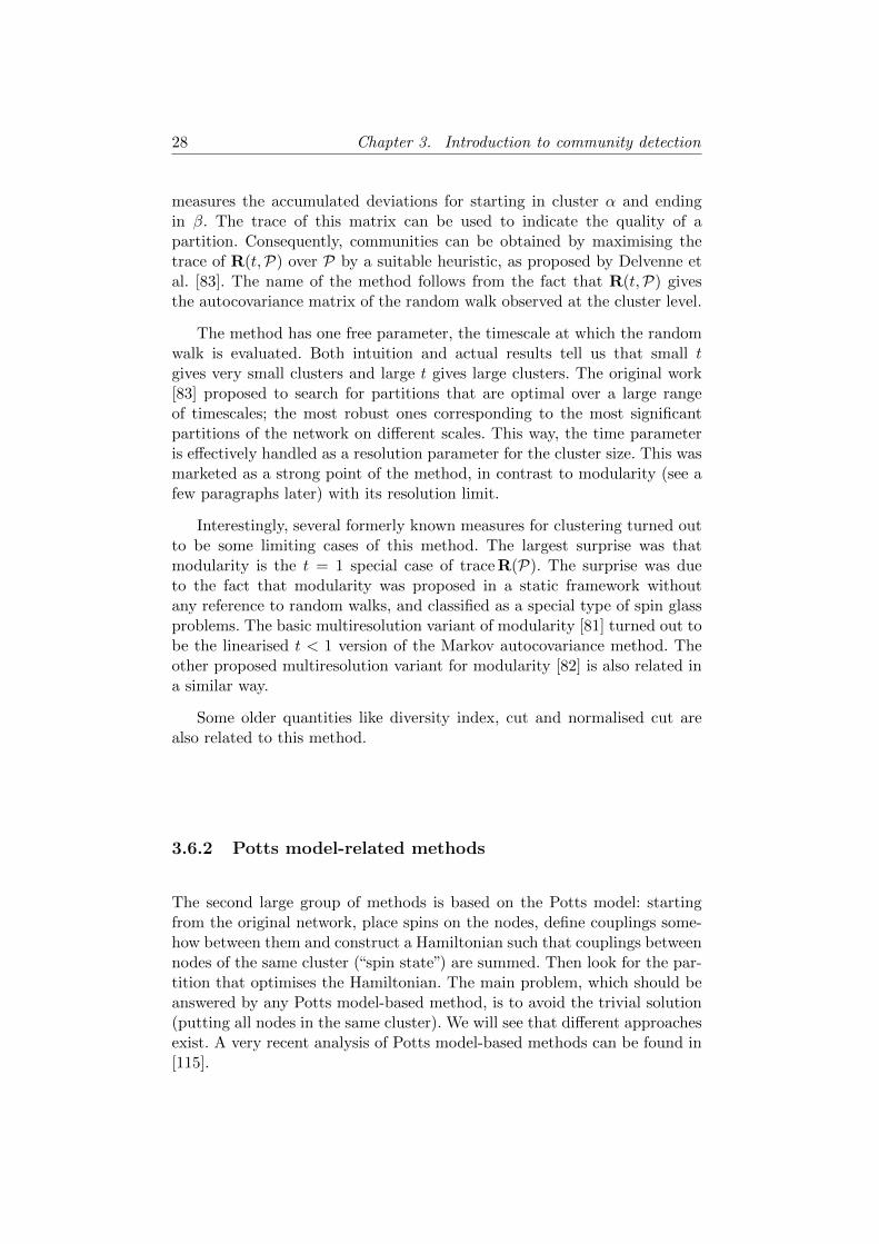
3.6.2 Potts model-related methods
The second large group of methods is based on the Potts model: startingfrom the original network, place spins on the nodes, define couplings some-how between them and construct a Hamiltonian such that couplings betweennodes of the same cluster (“spin state”) are summed. Then look for the par-tition that optimises the Hamiltonian. The main problem, which should beanswered by any Potts model-based method, is to avoid the trivial solution(putting all nodes in the same cluster). We will see that different approachesexist. A very recent analysis of Potts model-based methods can be found in[115].
3.6. Overview of the current methods 29
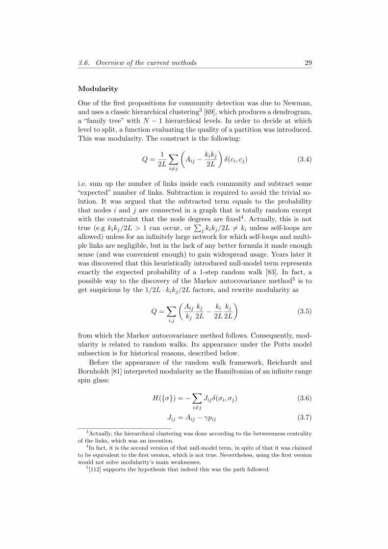
Modularity
One of the first propositions for community detection was due to Newman,and uses a classic hierarchical clustering3 [69], which produces a dendrogram,a “family tree” with N − 1 hierarchical levels. In order to decide at whichlevel to split, a function evaluating the quality of a partition was introduced.This was modularity. The construct is the following:
Q =1
2L
∑i 6=j
(Aij −
kikj2L
)δ(ci, cj) (3.4)
i.e. sum up the number of links inside each community and subtract some“expected” number of links. Subtraction is required to avoid the trivial so-lution. It was argued that the subtracted term equals to the probabilitythat nodes i and j are connected in a graph that is totally random exceptwith the constraint that the node degrees are fixed4. Actually, this is nottrue (e.g kikj/2L > 1 can occur, or
∑j kikj/2L 6= ki unless self-loops are
allowed) unless for an infinitely large network for which self-loops and multi-ple links are negligible, but in the lack of any better formula it made enoughsense (and was convenient enough) to gain widespread usage. Years later itwas discovered that this heuristically introduced null-model term representsexactly the expected probability of a 1-step random walk [83]. In fact, apossible way to the discovery of the Markov autocovariance method5 is toget suspicious by the 1/2L · kikj/2L factors, and rewrite modularity as
Q =∑i,j
(Aijkj
kj2L− ki
2L
kj2L
)(3.5)
from which the Markov autocovariance method follows. Consequently, mod-ularity is related to random walks. Its appearance under the Potts modelsubsection is for historical reasons, described below.
Before the appearance of the random walk framework, Reichardt andBornholdt [81] interpreted modularity as the Hamiltonian of an infinite rangespin glass:
H({σ}) = −∑i 6=j
Jijδ(σi, σj) (3.6)
Jij = Aij − γpij (3.7)
3Actually, the hierarchical clustering was done according to the betweenness centralityof the links, which was an invention.
4In fact, it is the second version of that null-model term, in spite of that it was claimedto be equivalent to the first version, which is not true. Nevertheless, using the first versionwould not solve modularity’s main weaknesses.
5[112] supports the hypothesis that indeed this was the path followed.
30 Chapter 3. Introduction to community detection
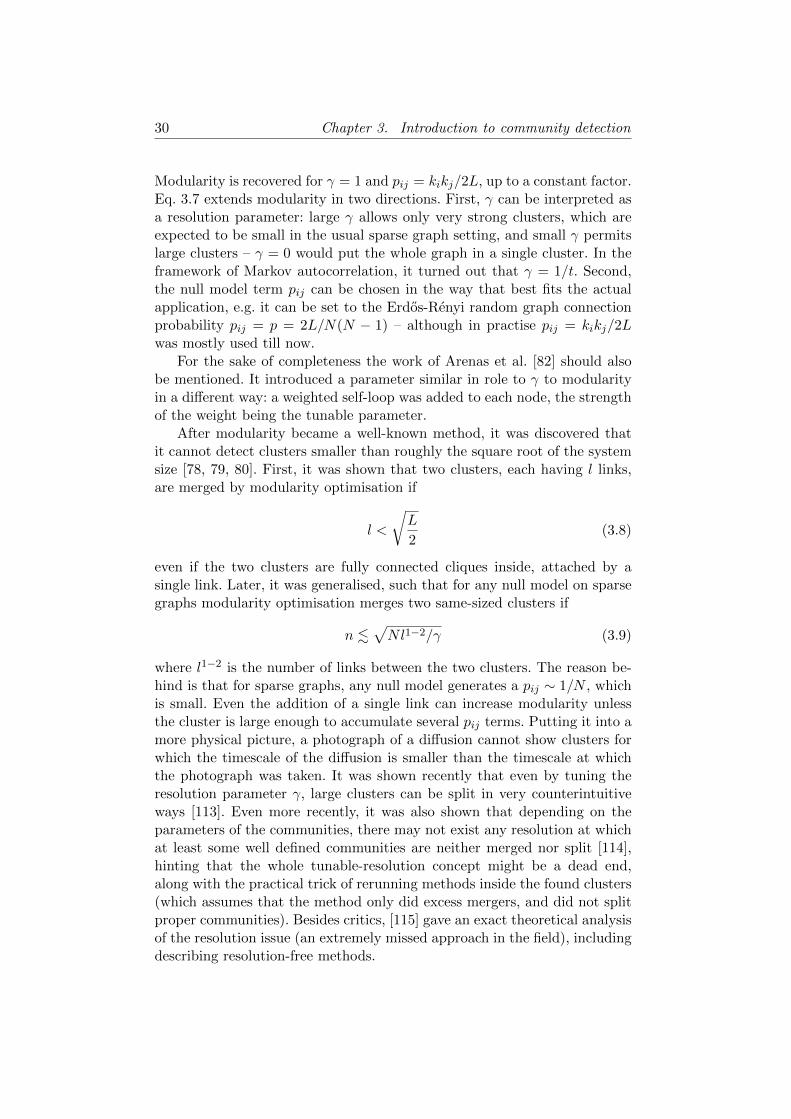
Modularity is recovered for γ = 1 and pij = kikj/2L, up to a constant factor.Eq. 3.7 extends modularity in two directions. First, γ can be interpreted asa resolution parameter: large γ allows only very strong clusters, which areexpected to be small in the usual sparse graph setting, and small γ permitslarge clusters – γ = 0 would put the whole graph in a single cluster. In theframework of Markov autocorrelation, it turned out that γ = 1/t. Second,the null model term pij can be chosen in the way that best fits the actualapplication, e.g. it can be set to the Erdos-Renyi random graph connectionprobability pij = p = 2L/N(N − 1) – although in practise pij = kikj/2Lwas mostly used till now.
For the sake of completeness the work of Arenas et al. [82] should alsobe mentioned. It introduced a parameter similar in role to γ to modularityin a different way: a weighted self-loop was added to each node, the strengthof the weight being the tunable parameter.
After modularity became a well-known method, it was discovered thatit cannot detect clusters smaller than roughly the square root of the systemsize [78, 79, 80]. First, it was shown that two clusters, each having l links,are merged by modularity optimisation if
l <
√L
2(3.8)
even if the two clusters are fully connected cliques inside, attached by asingle link. Later, it was generalised, such that for any null model on sparsegraphs modularity optimisation merges two same-sized clusters if
n .√Nl1−2/γ (3.9)
where l1−2 is the number of links between the two clusters. The reason be-hind is that for sparse graphs, any null model generates a pij ∼ 1/N , whichis small. Even the addition of a single link can increase modularity unlessthe cluster is large enough to accumulate several pij terms. Putting it into amore physical picture, a photograph of a diffusion cannot show clusters forwhich the timescale of the diffusion is smaller than the timescale at whichthe photograph was taken. It was shown recently that even by tuning theresolution parameter γ, large clusters can be split in very counterintuitiveways [113]. Even more recently, it was also shown that depending on theparameters of the communities, there may not exist any resolution at whichat least some well defined communities are neither merged nor split [114],hinting that the whole tunable-resolution concept might be a dead end,along with the practical trick of rerunning methods inside the found clusters(which assumes that the method only did excess mergers, and did not splitproper communities). Besides critics, [115] gave an exact theoretical analysisof the resolution issue (an extremely missed approach in the field), includingdescribing resolution-free methods.
3.6. Overview of the current methods 31
A practical workaround to this resolution problem, originally aiming to pro-vide a very fast modularity optimisation, called Louvain method, was intro-duced by [62]. It applies a renormalisation-like technique: initially all nodesare placed in separate communities, and a fast greedy (downhill) optimisa-tion finds a locally optimal solution. Because the optimisation allows onlysingle-node movements, the formation of large clusters is avoided. Then,communities are merged into super-nodes and the optimisation is appliedagain. This procedure is iterated until ending up in a single cluster con-taining all nodes. This way, a hierarchy of communities is obtained, andlow levels can contain communities below the resolution limit of modularity.The result depends on the order of the nodes, thus the method should beconsidered a stochastic one. Consequently, several runs may be required forreaching a deep local optimum. Although it does not resolve the theoreticalproblems of modularity, it is a notable method: it provided early a practicalworkaround to the resolution limit, along with very short running times andit is the best performer on the current benchmarks among modularity-basedmethods [96].
Link partitioning by modularity
Usually, methods try to partition the nodes in the network. However, asEvans and Lambiotte [117] pointed out, it may also worth to partition thelinks instead. This way, overlaps between clusters can be obtained easily. Forpartitioning, modularity was proposed with proper modifications, especiallyin the null model term.
Method of Ronhovde & Nussinov
Another Potts model was proposed by Ronhovde and Nussinov [119]. Itsuggested
H({σ}) = −1
2
∑i 6=j
(aijAij − γbij(1−Aij))δ(σi, σj) (3.10)
For unweighted graphs aij = bij = 1. The Hamiltonian optimises for linkdensity inside the clusters. Due to the lack of any global parameters in H,it has no resolution limit problem tied to the system size, in contrast tomodularity. Still, it has a resolution parameter (again called γ), regulatinghow strongly the missing links are penalised (compared to the reward forexisting links). As for sparse graphs the large communities have lower edgedensities than the small ones, γ tunes the size scale of the found clusters.
For finding the most relevant γ values, [119] proposed a spin glass-inspired method. The Hamiltonian should be optimised several times, andthe found local optima should be compared using some similarity measure.The ansatz is that the graph has a single well-defined partition, and at the
32 Chapter 3. Introduction to community detection
resolution fitting to that true partition the different runs all give the sameanswer. Therefore, one should look for the γ value for which the similarityof the found partitions has a peak.
It should be noted that well before [119] appeared, Nepusz et al. devel-oped a method for detecting fuzzy communities, i.e. clusters for which themembership of the nodes can be arbitrary real number between 0 and 1[120]. It is easy to show that when the fuzzy memberships are replaced bythe conventional 0-or-1 type and the network is unweighted, the method isequivalent to eq. 3.10, using γ = 1, aij = bij = 1.
Stochastic blockmodels
Stochastic blockmodels are usually not inspired by Potts models or spinglasses, however they usually do correspond to the optimisation of a functionconsisting of couplings between nodes in the same/different clusters. As anillustrative example, the blockmodel of Hofman and Wiggins [121] describesa multinomial distribution for the cluster assignments of the nodes andBernoulli distributions for the presence/absence of the links, the intra-clusterand inter-cluster links having different probabilities. In other words, themodel builds a random graph of K clusters with prescribed sizes by rollinga K sided die, biased by the cluster sizes (denoted by the K-componentvector ~n), to determine the node memberships. Then all intra-cluster linksare drawn with probability ϑc and all inter-cluster links with probability ϑd.Then the total probability of a particular graph with a particular clusterstructure is
p(A, ~σ|~n, ϑc, ϑd) = ϑc+c (1− ϑc)c−ϑd+d (1− ϑd)d−K∏µ=1
(nµN
)nµ= (3.11)
c+ =∑i>j
Aijδσi,σj d+ =∑i>j
Aij(1− δσi,σj ) (3.12)
c− =∑i>j
(1−Aij)δσi,σj d− =∑i>j
(1−Aij)(1− δσi,σj ) (3.13)
Now the community detection method consists in finding the cluster config-uration ~σ which maximises eq. 3.11, or alternatively, which minimises the
3.6. Overview of the current methods 33
Hamiltonian
H = − ln p(A, ~σ|~n, ϑc, ϑd) = −∑i<j
(JLAij − JG)δσi,σj −K∑µ=1
nµ ln(nµ/N) =
= −∑i<j
[(JL − JG)Aij − JG(1−Aij)] δσi,σj −K∑µ=1
nµ ln(nµ/N)
(3.14)
JG = ln1− ϑd1− ϑc
(3.15)
JC = lnϑcϑd
+ JG (3.16)
which is indeed a K-state Potts Hamiltonian equipped with chemical po-tentials. Interestingly, the Potts model of Ronhovde and Nussinov [119] is aspecial case, without the chemical potential terms.
Several other blockmodels exist. E.g. the one of Hastings [122] is also aspecial case of the Hofman-Wiggins model. The“mixture model”of Newmanand Leicht [123] uses soft (fuzzy) memberships and a finer set of couplingsdefined for node-cluster pairs, also including the inter-cluster links. Onlyexisting links are taken into account. Wang and Lai [124] improved theNewman-Leicht model by incorporating terms for the missing links. Themodel of McDaid and Hurley [125] also applies soft memberships, in order todetect strongly overlapping clusters. The blockmodel of Karrer and Newman[126] counts only for the existing links, but takes into account the inter-cluster links also. A quite similar object was proposed by Bickel and Chen[127], without naming it a blockmodel. Interestingly, this latter method canpotentially used for detecting bipartite structures also, i.e. classes withinwhich links are very rare.
Label propagation
A route different from the above ones was taken by Raghavan et al. Insteadof a function to be optimised, they defined a simple intuitive dynamics onthe graph: initially all nodes have different “labels“ (or colours or spin states. . . ), and turn-by-turn, each node adopts the label most frequently occurringamong its neighbours. Ties are broken at random. Communities are definedby the labels in the stationary state in which no node’s label changes. Themethod is local (no global parameters are used), parameter-free and worksvery fast, essentially in linear time – it was reported that 5 turns are usuallyenough, independently of the network size.
As we will see in Sec. 4.1, the dynamics above is equivalent to the find-ing of a local optimum of a zero-temperature Potts model [92]. While beingtrapped in a higher local minimum is usually regarded as a problem which

34 Chapter 3. Introduction to community detection
should be avoided, here it is applied as an alternative way to escape the triv-ial ground state of the Potts model associated with a graph. In fact, a deeplocal minimum close to the ground state in energy is in fact undesirable,because it most probably just splits a handful of nodes off from the hugecluster containing all the other nodes. Apart from this observation, the en-ergy of a local minimum itself cannot be used to characterise the quality of aclustering. Which leads us to the real problem of the method: unfortunately,the number of higher local minima is very high, rendering the method lessstable than desired. E.g. a network of 34 nodes has at least 518 differentsolutions [92].
Nevertheless, the method proved quite popular, and different variationsappeared: overlapping clusters by allowing more labels for a node [128],introducing simple constraints [129], and attenuating hops with distancefrom the origin [130].
3.6.3 Percolation-related methods
Although the word ”cluster“ is strongly associated with percolation for sta-tistical physicists, the plain percolation problem in itself is unsuited forcommunity detection – percolation clusters are stochastic objects, and itis not trivial how to relate them to dense subgraphs. Nevertheless, thereare some methods related to percolation. Note: it also means that proposedcommunity detection methods cover the possible parameter values of theFortuin-Kasteleyn formalism [133], q = 1 by percolation and q > 1 by Pottsmodel.
Clique Percolation
A radically different approach (from quality functions like modularity) forcommunity detection was introduced in 2005 by Palla et al. [74]. It definescommunities as connected components/percolation clusters, but not on theactual graph. Instead, it builds a graph of adjacent k-cliques of the origi-nal graph. Adjacency of two k-cliques are defined by sharing k − 1 nodes.k is a parameter for the method, usually set just under the critical pointfor percolation, i.e. k is minimal with the restriction that there is no perco-lating k-clique cluster. The method has important advantages: it is totallydeterministic, in contrast to the heuristic optimisation methods e.g. for mod-ularity; it is fast in practise; and it naturally allows for overlapping clusters.Clique Percolation does not force necessarily all nodes to belong to any clus-ter – later it was realised that it can be an important feature [91]. However,its applicability depends on the edge densities in the network. Furthermore,the requirement of rolling cliques seems to be too restrictive in some cases.Clique Percolation was also extended to weighted and directed graphs aswell [134, 135].
3.6. Overview of the current methods 35
Thresholding
Although requiring weighted graphs, a very simple method is to define athreshold, remove edges having weights below the threshold, and define thecommunities as the connected components. Being very straightforward toimplement, the choice of the threshold is far from trivial [136]; it may hap-pen that different clusters have different individual thresholds. Furthermore,thresholding defines clusters on the basis of the single weakest outside link,which is quite an oversimplification.
Hierarchical random graph fitting method
A more sophisticated thresholding-like method was introduced by Clausetet al. [137]. It builds a dendrogram, which lowest level nodes or “leaves”are the nodes of the real network, and higher level nodes are subsets ofreal nodes. These higher level nodes in the dendrogram have an associatedprobability which tells us the probability of a link being present betweentwo real nodes which has the actual internal dendrogram node as the lowestcommon ancestor. Setting a threshold probability value cuts the dendrogramat the corresponding level, splitting the network into connected components,which can be interpreted as communities. The difficulty is the same as withthe standard thresholding procedure, one should decide the threshold valuesomehow.
3.6.4 Other
There are several other methods outside the ones based on the traditionalmodels of statistical physics. Most of them are just heuristic ideas withoutsupporting background (like the Label propagation was originally), otherones has more or less theory behind.
Weak & strong definition of Radicchi et al.
For defining communities, Radicchi et al. [138] proposed two possibilities.The subgraph C is a community “in the strong sense” if
kiin > kiout ∀i ∈ C (3.17)
Alternatively, the subgraph C is a community “in the weak sense” if∑i∈C
kiin >∑i∈C
kiout (3.18)
An interesting heuristic was also provided: start from the whole graph, andsequentially remove links in decreasing order of their betweennesses. If re-moving a link would result in a split such that the new clusters does not obey
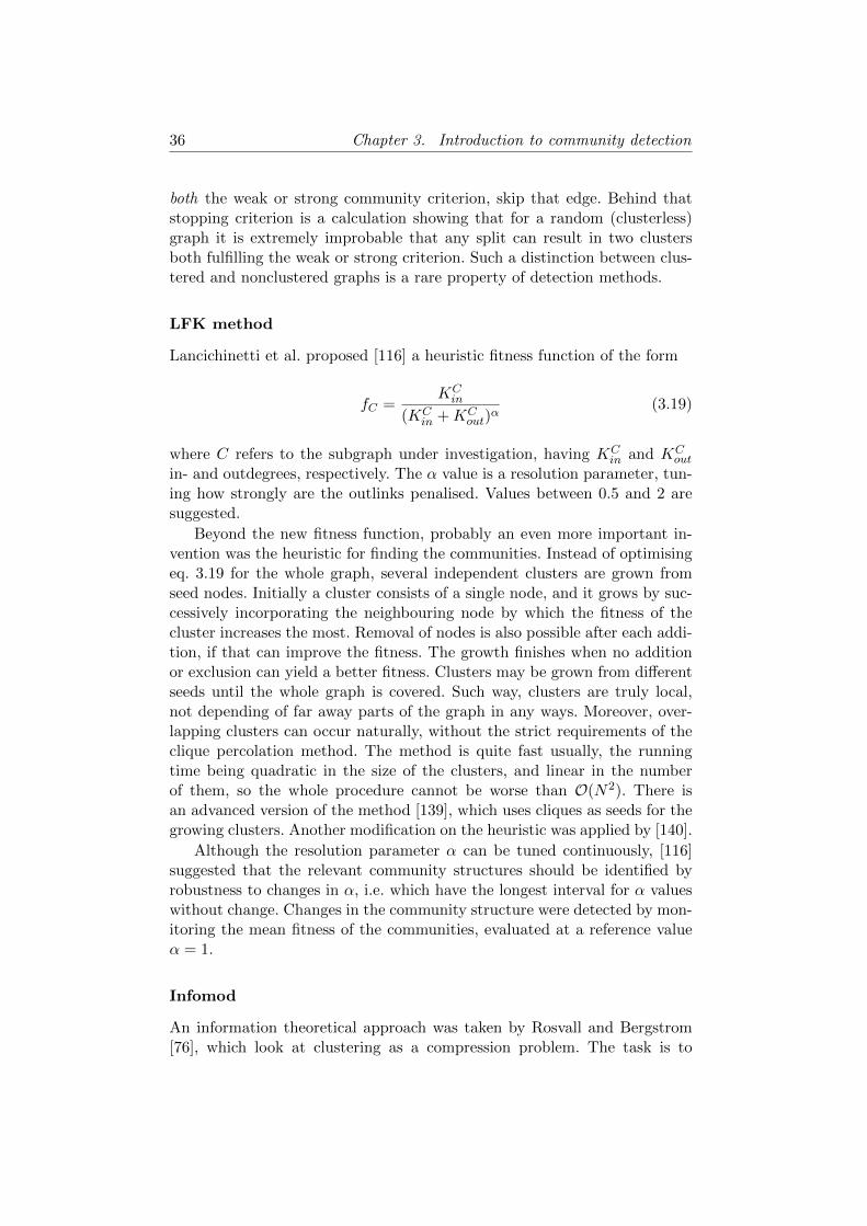
36 Chapter 3. Introduction to community detection
both the weak or strong community criterion, skip that edge. Behind thatstopping criterion is a calculation showing that for a random (clusterless)graph it is extremely improbable that any split can result in two clustersboth fulfilling the weak or strong criterion. Such a distinction between clus-tered and nonclustered graphs is a rare property of detection methods.
LFK method
Lancichinetti et al. proposed [116] a heuristic fitness function of the form
fC =KCin
(KCin +KC
out)α
(3.19)
where C refers to the subgraph under investigation, having KCin and KC
out
in- and outdegrees, respectively. The α value is a resolution parameter, tun-ing how strongly are the outlinks penalised. Values between 0.5 and 2 aresuggested.
Beyond the new fitness function, probably an even more important in-vention was the heuristic for finding the communities. Instead of optimisingeq. 3.19 for the whole graph, several independent clusters are grown fromseed nodes. Initially a cluster consists of a single node, and it grows by suc-cessively incorporating the neighbouring node by which the fitness of thecluster increases the most. Removal of nodes is also possible after each addi-tion, if that can improve the fitness. The growth finishes when no additionor exclusion can yield a better fitness. Clusters may be grown from differentseeds until the whole graph is covered. Such way, clusters are truly local,not depending of far away parts of the graph in any ways. Moreover, over-lapping clusters can occur naturally, without the strict requirements of theclique percolation method. The method is quite fast usually, the runningtime being quadratic in the size of the clusters, and linear in the numberof them, so the whole procedure cannot be worse than O(N2). There isan advanced version of the method [139], which uses cliques as seeds for thegrowing clusters. Another modification on the heuristic was applied by [140].
Although the resolution parameter α can be tuned continuously, [116]suggested that the relevant community structures should be identified byrobustness to changes in α, i.e. which have the longest interval for α valueswithout change. Changes in the community structure were detected by mon-itoring the mean fitness of the communities, evaluated at a reference valueα = 1.
Infomod
An information theoretical approach was taken by Rosvall and Bergstrom[76], which look at clustering as a compression problem. The task is to
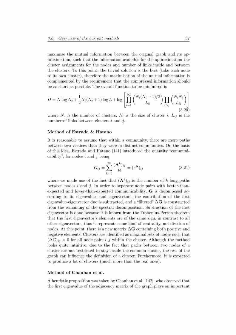
3.6. Overview of the current methods 37
maximise the mutual information between the original graph and its ap-proximation, such that the information available for the approximation thecluster assignments for the nodes and number of links inside and betweenthe clusters. To this point, the trivial solution is the best (take each nodeto its own cluster), therefore the maximisation of the mutual information iscomplemented by the requirement that the compressed information shouldbe as short as possible. The overall function to be minimised is
D = N logNc +1
2Nc(Nc + 1) logL+ log
Nc∏i=1
(Ni(Ni − 1)/2
Lii
)∏i>j
(NiNj
Lij
)(3.20)
where Nc is the number of clusters, Ni is the size of cluster i, Lij is thenumber of links between clusters i and j.
Method of Estrada & Hatano
It is reasonable to assume that within a community, there are more pathsbetween two vertices than they were in distinct communities. On the basisof this idea, Estrada and Hatano [141] introduced the quantity “communi-cability”, for nodes i and j being
Gij =
∞∑k=0
(Ak)ijk!
= (eA)ij (3.21)
where we made use of the fact that (Ak)ij is the number of k long pathsbetween nodes i and j. In order to separate node pairs with better-than-expected and lower-than-expected communicability, G is decomposed ac-cording to its eigenvalues and eigenvectors, the contribution of the firsteigenvalue-eigenvector duo is subtracted, and a “filtered” ∆G is constructedfrom the remaining of the spectral decomposition. Subtraction of the firsteigenvector is done because it is known from the Frobenius-Perron theoremthat the first eigenvector’s elements are of the same sign, in contrast to allother eigenvectors, thus it represents some kind of centrality, not division ofnodes. At this point, there is a new matrix ∆G containing both positive andnegative elements. Clusters are identified as maximal sets of nodes such that(∆G)ij > 0 for all node pairs i, j within the cluster. Although the methodlooks quite intuitive, due to the fact that paths between two nodes of acluster are not restricted to stay inside the common cluster, the rest of thegraph can influence the definition of a cluster. Furthermore, it is expectedto produce a lot of clusters (much more than the real ones).
Method of Chauhan et al.
A heuristic proposition was taken by Chauhan et al. [142], who observed thatthe first eigenvalue of the adjacency matrix of the graph plays an important
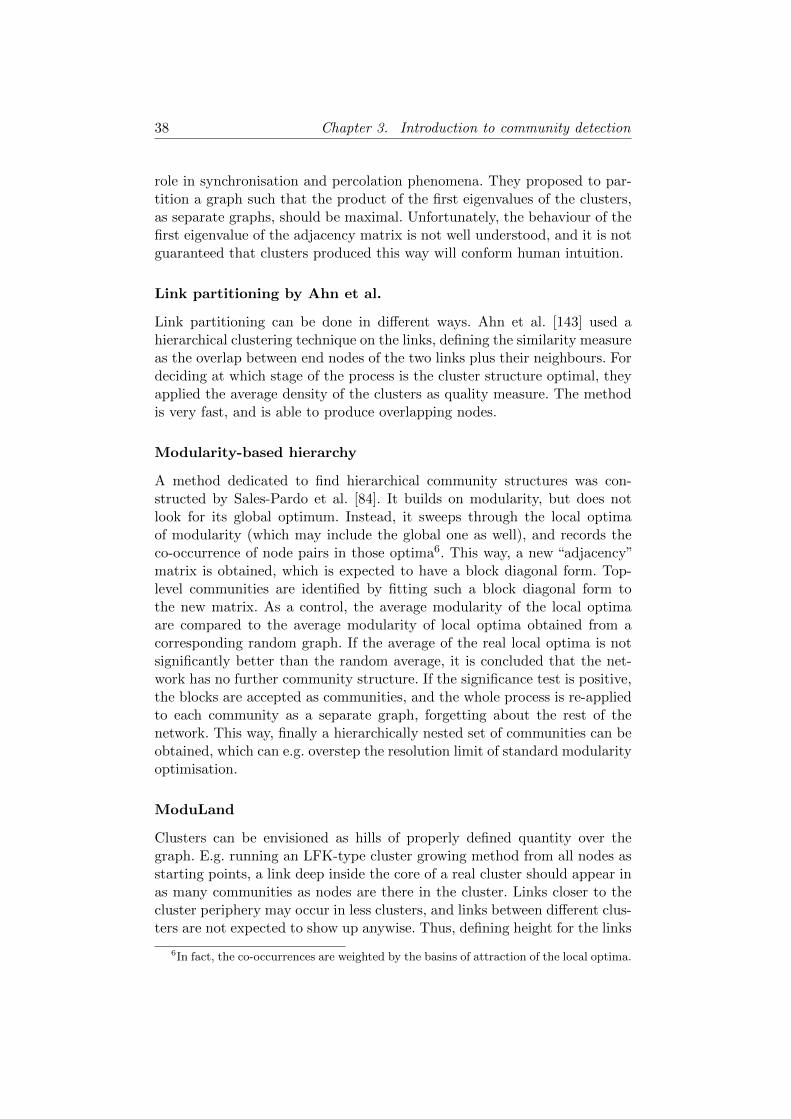
38 Chapter 3. Introduction to community detection
role in synchronisation and percolation phenomena. They proposed to par-tition a graph such that the product of the first eigenvalues of the clusters,as separate graphs, should be maximal. Unfortunately, the behaviour of thefirst eigenvalue of the adjacency matrix is not well understood, and it is notguaranteed that clusters produced this way will conform human intuition.
Link partitioning by Ahn et al.
Link partitioning can be done in different ways. Ahn et al. [143] used ahierarchical clustering technique on the links, defining the similarity measureas the overlap between end nodes of the two links plus their neighbours. Fordeciding at which stage of the process is the cluster structure optimal, theyapplied the average density of the clusters as quality measure. The methodis very fast, and is able to produce overlapping nodes.
Modularity-based hierarchy
A method dedicated to find hierarchical community structures was con-structed by Sales-Pardo et al. [84]. It builds on modularity, but does notlook for its global optimum. Instead, it sweeps through the local optimaof modularity (which may include the global one as well), and records theco-occurrence of node pairs in those optima6. This way, a new “adjacency”matrix is obtained, which is expected to have a block diagonal form. Top-level communities are identified by fitting such a block diagonal form tothe new matrix. As a control, the average modularity of the local optimaare compared to the average modularity of local optima obtained from acorresponding random graph. If the average of the real local optima is notsignificantly better than the random average, it is concluded that the net-work has no further community structure. If the significance test is positive,the blocks are accepted as communities, and the whole process is re-appliedto each community as a separate graph, forgetting about the rest of thenetwork. This way, finally a hierarchically nested set of communities can beobtained, which can e.g. overstep the resolution limit of standard modularityoptimisation.
ModuLand
Clusters can be envisioned as hills of properly defined quantity over thegraph. E.g. running an LFK-type cluster growing method from all nodes asstarting points, a link deep inside the core of a real cluster should appear inas many communities as nodes are there in the cluster. Links closer to thecluster periphery may occur in less clusters, and links between different clus-ters are not expected to show up anywise. Thus, defining height for the links
6In fact, the co-occurrences are weighted by the basins of attraction of the local optima.
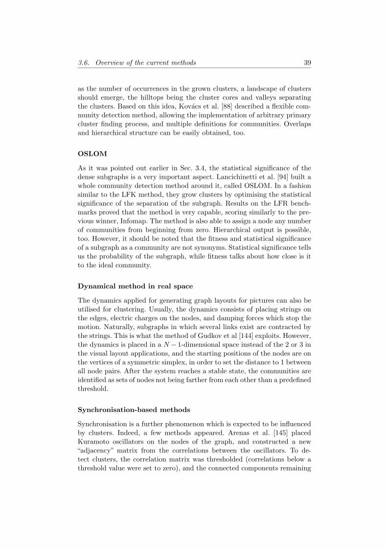
3.6. Overview of the current methods 39
as the number of occurrences in the grown clusters, a landscape of clustersshould emerge, the hilltops being the cluster cores and valleys separatingthe clusters. Based on this idea, Kovacs et al. [88] described a flexible com-munity detection method, allowing the implementation of arbitrary primarycluster finding process, and multiple definitions for communities. Overlapsand hierarchical structure can be easily obtained, too.
OSLOM
As it was pointed out earlier in Sec. 3.4, the statistical significance of thedense subgraphs is a very important aspect. Lancichinetti et al. [94] built awhole community detection method around it, called OSLOM. In a fashionsimilar to the LFK method, they grow clusters by optimising the statisticalsignificance of the separation of the subgraph. Results on the LFR bench-marks proved that the method is very capable, scoring similarly to the pre-vious winner, Infomap. The method is also able to assign a node any numberof communities from beginning from zero. Hierarchical output is possible,too. However, it should be noted that the fitness and statistical significanceof a subgraph as a community are not synonyms. Statistical significance tellsus the probability of the subgraph, while fitness talks about how close is itto the ideal community.
Dynamical method in real space
The dynamics applied for generating graph layouts for pictures can also beutilised for clustering. Usually, the dynamics consists of placing strings onthe edges, electric charges on the nodes, and damping forces which stop themotion. Naturally, subgraphs in which several links exist are contracted bythe strings. This is what the method of Gudkov et al [144] exploits. However,the dynamics is placed in a N − 1-dimensional space instead of the 2 or 3 inthe visual layout applications, and the starting positions of the nodes are onthe vertices of a symmetric simplex, in order to set the distance to 1 betweenall node pairs. After the system reaches a stable state, the communities areidentified as sets of nodes not being farther from each other than a predefinedthreshold.
Synchronisation-based methods
Synchronisation is a further phenomenon which is expected to be influencedby clusters. Indeed, a few methods appeared. Arenas et al. [145] placedKuramoto oscillators on the nodes of the graph, and constructed a new“adjacency” matrix from the correlations between the oscillators. To de-tect clusters, the correlation matrix was thresholded (correlations below athreshold value were set to zero), and the connected components remaining
40 Chapter 3. Introduction to community detection
were declared as communities. As a function of the threshold, a hierarchicalstructure was obtained.
Boccaletti et al. [146] defined a similar model with some modifications,most importantly the couplings between the oscillators were weighted by thecorresponding edge betweennesses. From the resulting hierarchy of commu-nities the optimal partition was selected applying modularity.
Li et al. [147] used a different oscillator model, but also constructed acorrelation matrix for the oscillators. The correlation matrix was clusteredusing k-means clustering.
3.7 Results & applications so far
After almost a decade of research, the problem of finding locally dense sub-graphs is clearly not solved, but very significant advancements were achieved.Most importantly, the ambition to handle the clustering problem in a verygeneral setting appeared, any application-specific information being cut off.In certain scenarios, very good answers were already found (Infomap forpartitioning). For harder problems (overlapping clusters, hierarchy, etc.), weare in the brainstorming stage, with lots of different ideas.Another very important issue is the demand for testing. Clustering methodshave been appearing for decades, but really useful methods to judge theirperformance were lacking. The fact that the research community is not sat-isfied with this situation7, as well as the appearance of the LFR benchmarkfamily are significant steps forward. Although there is a lot to do (see Sec.3.4), the improvements are promising. Similar is true for the question ofsignificance of the results.
Till now, most of the effort has been concentrated on the development ofmethods, and a generally accepted definition of communities is still lacking.Therefore it is not surprising that meaningful applications are very scarce.However, attempts exist. E.g. [148] investigated various statistical features ofempirical community structures for different types of networks (biological,infrastructural, etc.), using multiple detection methods for robust results.The effect of topological inhomogeneities on spreading processes [149] andsynchronisation [150] was also examined, signing that all problems for whichthe separation of time scales is important are potential applications.Concerning social networks, applying clique percolation to a huge mobilephone call network in consecutive months showed an interesting differencebetween the dynamics of small and large groups [151]. Small groups tendedto have long lifespan if their members remained the same, in contrast to largegroups which tended to persist when members changed more frequently. Thecrossover size was around a few dozen nodes. Another study [152] focused onschool friendship networks from the US, revealing the mixing preferences of
7which is very comfortable, since new methods can be published unboundedly
3.7. Results & applications so far 41
different ethnic groups. Clusters of similarly voting members were identifiedin the United Nations General Assembly (1946-2008) [153] and in the USSenate (1789-2008) [154].In biology, community detection was applied to predict functions of pro-teins and also new functional clusters [155], to characterise different protein-protein interaction networks [156], to identify functional groups in metabolicnetworks [157], and to understand certain features of food webs [158]. Clus-ters of biology-related articles in the journal Proceedings of the NationalAcademy of Sciences of the USA were also analysed, in order to propose abetter article classification scheme [159].Community detection was also applied to potential energy landscapes ofLennard-Jones clusters [160], and to the identification of structures in glassesand amorphous materials [162, 163]. Sound propagation in granular materialwas connected to the cluster structure of force networks [164].
Beyond academic research, various companies experiment with the ap-plication of clustering, like telecommunication equipment manufacturers toachieve more effective network designs (see chapter 6), or financial invest-ment companies to diversify better their portfolio in terms of risk [165].
Even spin-off firms appeared, providing network analysis (communitydetection in the first place)-based services to customers (Maven7 by TamasVicsek’s group, PrediNet by Peter Csermely’s group).
Chapter 4
Analysis of a few communitydetection methods
In this chapter, a few community detection methods are investigated, es-pecially from the point of view of application to real networks. First, someinteresting properties of the label propagation method are presented. Then,eigenvectors of a financial correlation matrix are investigated. Finally, em-pirical comparison of some influential methods are made.
4.1 Properties of the label propagation method
Raghavan et al. suggested a method for detecting communities called labelpropagation [77]. It defines a community as a set of nodes such that eachnode has at least as many neighbours in its own community as in any otherone. In the initial stage of the method, all nodes form a distinct community(each node has its own “label”). Then, at each timestep, the nodes jointhat community to which the largest fraction of their neighbours belong,by adopting the corresponding label. If there are multiple choices, a randomdecision is made with uniform distribution. The method produces a partitionvery fast: the algorithm is linear in the number of nodes on sparse graphs,and it was found that in most cases, 5 iterations are enough to reach almostfull convergence, irrespective of the size of the graph.
Because of its conceptual simplicity and speed, the label propagationmethod proved popular [128]-[131]. To “conceptual simplicity”, it will beshown in the next paragraphs that label propagation is correspond to awell-known model in statistical physics, i.e. it is equivalent to finding thelocal minima of a zero-temperature kinetic Potts model. To “speed”, it willturn out that the method should be run several times, possibly much morethan the number of nodes.
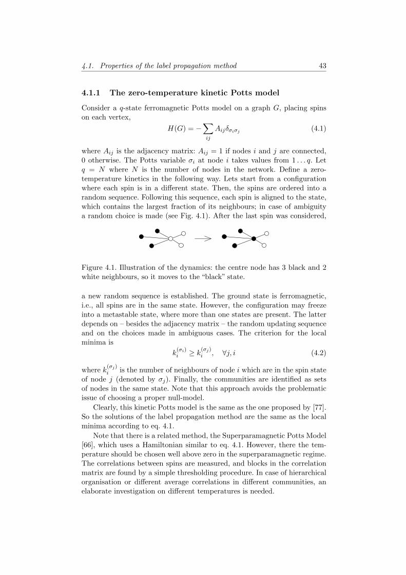
4.1. Properties of the label propagation method 43
4.1.1 The zero-temperature kinetic Potts model
Consider a q-state ferromagnetic Potts model on a graph G, placing spinson each vertex,
H(G) = −∑ij
Aijδσiσj (4.1)
where Aij is the adjacency matrix: Aij = 1 if nodes i and j are connected,0 otherwise. The Potts variable σi at node i takes values from 1 . . . q. Letq = N where N is the number of nodes in the network. Define a zero-temperature kinetics in the following way. Lets start from a configurationwhere each spin is in a different state. Then, the spins are ordered into arandom sequence. Following this sequence, each spin is aligned to the state,which contains the largest fraction of its neighbours; in case of ambiguitya random choice is made (see Fig. 4.1). After the last spin was considered,
Figure 4.1. Illustration of the dynamics: the centre node has 3 black and 2white neighbours, so it moves to the “black” state.
a new random sequence is established. The ground state is ferromagnetic,i.e., all spins are in the same state. However, the configuration may freezeinto a metastable state, where more than one states are present. The latterdepends on – besides the adjacency matrix – the random updating sequenceand on the choices made in ambiguous cases. The criterion for the localminima is
k(σi)i ≥ k(σj)
i , ∀j, i (4.2)
where k(σj)i is the number of neighbours of node i which are in the spin state
of node j (denoted by σj). Finally, the communities are identified as setsof nodes in the same state. Note that this approach avoids the problematicissue of choosing a proper null-model.
Clearly, this kinetic Potts model is the same as the one proposed by [77].So the solutions of the label propagation method are the same as the localminima according to eq. 4.1.
Note that there is a related method, the Superparamagnetic Potts Model[66], which uses a Hamiltonian similar to eq. 4.1. However, there the tem-perature should be chosen well above zero in the superparamagnetic regime.The correlations between spins are measured, and blocks in the correlationmatrix are found by a simple thresholding procedure. In case of hierarchicalorganisation or different average correlations in different communities, anelaborate investigation on different temperatures is needed.
44 Chapter 4. Analysis of a few community detection methods
It is straightforward to extend the method for weighted graphs, where theweights can be based on e.g. traffic/capacity, betweenness centrality [167],or other measures.
4.1.2 Analysis of the label propagation method
The zero-temperature kinetic model was investigated earlier on lattices [168],[169], [170]. It was reported that such dynamics may also end up in metastablestates, instead of the ground state. In the q = 2 (Ising) case on the squarelattice, the systems freezes in parallel stripes, with different alignment ofspins in neighbouring stripes, with probability p ≈ 1/3 in 2D. On latticeswith odd coordination number, finite frozen islands are also possible. Inhigher dimensions, the system will circulate forever over equienergetic con-figurations (“blinking” states), with p→ 1, as the number of spins diverges.Similar observations were made for q > 2. So on regular graphs, the dynam-ics described in the previous subsection also leads to communities which areclearly irrelevant.Although the high degree of symmetry makes the regular lattices very differ-ent from complex networks, regarding the possible metastable states, thesefindings indicate that it is important to check the relevance of the results,e.g. by comparing the outcomes of runs with different random number se-quences.
The kinetic Potts method described in the previous subsection was ap-plied to 2 real-world network, the Zachary karate club [101] and the proteininteraction network [171]. As there may be many local minima, the algo-rithm was run several times on both datasets. In such situations, one shoulddecide whether the actual local minimum was already found earlier. In or-der to save time, instead of comparing directly the two community sets, thequantity Q = 4L2 · Q for the two configurations were compared, where Qis the modularity [172], and L is the number of links in the network. If theQ values were exactly the same, the two configurations were judged as be-ing identical. Although improbable, it is theoretically possible that differentconfigurations have the same modularity value. Thus the obtained numbersare lower bounds of the numbers of the visited different local minima.
The most prominent feature of the results is the proliferation of the lo-cal minima: the algorithm found 518 different local minima (excluding theglobal one) out of 106 runs for the karate club network (consisting of 34nodes), and 129691 out of 2.2 × 10⁵ runs for the PIN (2111 nodes). As thelast new local minima were found in the 990767th and in the 219999th runs,respectively, most probably the limit has not been reached.The phenomenon that usually there are more local minima was also noticedby [77]. However, the solutions they found were quite similar the major-ity of the networks, therefore the fact that there are more than one wasjudged as unimportant. Moreover, it was not realised how large the num-
4.1. Properties of the label propagation method 45
ber of the solutions is. However, such a huge number of possible solutionssuggests an exhaustive exploration, which requires much more CPU timethan the O(number of links) time of a single run. The analysis of the resultsobviously requires a systematic and algorithmic investigation, which is nota straightforward task.
Reference [77] also proposed an aggregation method for checking the sim-ilarity of different solutions. It consists of assigning the same ‘aggregated’label to nodes which appeared always in the same community in n differentsolutions. Then a different aggregate should be made from n another solu-tions. Finally, a similarity measure should be calculated between the twosets of aggregate labels. Such aggregates were reported to be quite similar,therefore using an aggregate instead of an arbitrarily chosen single solutionwas suggested.
However, for the Zachary network, combining the solutions gives a resultvery close to the initial state of the label propagation method, i.e. placingeach node into a different community (3 communities of 2 members and 1 of3 remained). A similar tendency was observed on the PIN – by aggregatingall solutions, 94% of the nodes belong to communities not bigger than 10nodes (and there is only one community larger than 14 nodes). So one shoulddecide how many solutions to aggregate, which in turn determines the sizesof the communities, or the scale of the investigation, in other words, suchthat aggregating more solutions gives smaller communities.
4.1.3 Conclusions
I have shown that the label propagation method is equivalent to finding thelocal energy minima of a simple zero-temperature kinetic Potts model. Thenumber of local minima of two real-world networks turned out to be verylarge; it exceeds considerably the number of the nodes in the networks. Thisfeature suggests that the configurations corresponding to the local minimaneed further investigation. Aggregating the configurations tends to decon-struct the communities into very small units, depending on the number ofthe aggregated configurations. Therefore, serious questions arise about theapplicability of the label propagation method; for which there are a fewattempts to answer [129], [131], [132].
46 Chapter 4. Analysis of a few community detection methods
4.2 Communities in financial correlation matrices
4.2.1 Introduction
The network approach is a natural one for several complex systems. Formany systems, however, the nature of interactions is hidden and only someactivities of the nodes can be measured, e.g., in the form of time series.For such systems, the natural network representation is a complete graphwith weights corresponding to the elements of the correlation matrix deter-mined by the nodal activities. Then the task is to filter out from the noisycorrelation matrix the groups of closely related elements. This problem isquite general and it appears in many fields of research ranging from theevaluation of micro-array data to portfolio optimisation. In this chapter,correlation matrices of stock returns are studied.
Correlations between time-series of stock returns serve as one of the maininputs in the portfolio optimisation theory. In the classical Markowitz port-folio optimisation the correlations are used as measures of the dependencebetween the time series and the variance as the measure of risk [180].1 Asthe empirical time series are always finite, the resulting correlation matrixis noisy. This brings up the need to reduce the noise, for which the mostfrequently applied tool in the financial literature is principal componentanalysis [105].
Previously, correlation matrices of stock return time series have beenstudied from the network point of view, e.g., by using maximal spanningtrees (MST). The maximal spanning tree of a network is a tree containing allthe N nodes and N−1 links such that the sum of the weights is maximised. Itwas introduced in the study of financial correlation matrices by Mantegna[182], who was able to identify groups of stocks that make sense from aneconomic point of view. It was discovered that often, the branches of theMST correspond to business sectors or industries. Moreover, this methodenables to describe the hierarchical organisation of the market and has beenapplied to monitor the effect of the time dependence of the correlations[186] Later, MSTs of diverse financial correlation based networks have beenstudied, e.g., by Bonanno et al. [183, 184, 185] and Onnela et al. [186, 187].Indeed, the MST method is simple and gives reasonable results. However, itis too restrictive and thus other, complementary methods are needed.
In the so called asset graph approach, one ranks the links according to thevalues of the corresponding correlation matrix and considers only a fractionp of the strongest ones as occupied. By using this method for low values of pOnnela et al. [188] and Heimo et al. [189] found clear evidence of strong intra-business sector clustering. It has also been suggested that planar maximallyfiltered graphs yield a natural extension to the MST approach [190]. Otherinteresting approaches include methods based on the Superparamagnetic
1There are conceptual problems with this approach, which are not addressed here [181].

4.2. Communities in financial correlation matrices 47
Potts model [66] and on the maximum likelihood optimisation [191]. Severalfinancial markets have been studied from the above points of view.
Based on these approaches a following picture about the organisation ofthe correlation network of the stocks emerges: i) There is a dominant correla-tion among most of the stocks reflecting the overall behaviour of the market(this is the basis of the one factor model [181]); ii) The stocks are organisedhierarchically in clusters, which mainly correspond to industrial branches (asassumed in the multifactor models) [181] iii) There are systematic deviationsfrom this oversimplified picture, partly because of the ambiguous nature ofany classification scheme and partly because of inter-cluster relations; iv)In spite of considerable robustness in the correlations during the time of”business as usual”, major events like crashes cause dramatic changes in thenetwork structure [186].
All information on the network structure is encoded in its adjacencymatrix, or, for weighted networks, in the weight matrix. Likewise, all in-formation on the structure of correlations of stock returns is to be foundin the correlation matrix. Consequently, this information is also inheritedby the eigenvalues and eigenvectors of such matrices. If the data is struc-tured in terms of clusters and communities that these matrices represent, itshould also be reflected in the eigenpairs. For financial correlation matrices,it has been shown that most eigenpairs correspond to noise accessible byrandom matrix theory and thus the information about the cluster structureis contained in a few non-random eigenpairs [192, 193, 194] (see [195] foran overview). It was also suggested that clusters of highly correlated stockscould be identified by studying the localisation of non-random eigenvectors.
Here the eigenvectors of the weight and diffusion-related matrices derivedfrom stock price time series are investigated, from the point of view of clusterstructure.
The correlation matrix studied in this chapter is constructed from thelogarithmic returns of New York Stock Exchange (NYSE) traded stocks.The data consists of the daily closing prices of 476 stocks and ranges from2-Jan-1980 to 31-Dec-1999.
The chapter is organised as follows. Section 4.2.2 gives a short intro-duction to stock price-related matrices and their spectra. In Section 4.2.3,results corresponding to the first eigenvector of the weight matrix are pre-sented, and Section 4.2.4 analyses the intermediate eigenvectors of somematrices.
4.2.2 Basic notions
Matrices related to weighted networks
A simple undirected and weighted network can be represented by a weightmatrix W in which an element Wij = Wji (≥ 0 in this chapter) corresponds
48 Chapter 4. Analysis of a few community detection methods
to the weight of the link between the nodes i and j and the diagonal ele-ments are zero. Note that Wij = 0 signifies the absence of the link. The sumsi =
∑jWij is the strength of node i [196]. Here, the analysis is restricted to
irreducible networks, i.e., networks consisting of just one connected compo-nent. In this case the Frobenius-Perron theorem states that W has a largestpositive eigenvalue and the components of the corresponding eigenvector arenon-zero and of the same sign.
Diffusion process in terms of random walks can be used as a tool forstudying the structure of a network [97, 203, 204]. At each time step awalker moves at random from its current node j to node i with probabilityTij = Wij/sj . If we denote the walker density at node i by vi(t), the averagedynamics of the process is described by
~v(t+ 1) = T~v(t) (4.3)
or equivalently by~v(t+ 1)− ~v(t) = D~v(t), (4.4)
where ~v(t) = (v1(t), . . . , vN (t))T and D = T − I. Here, T denotes thetransfer matrix and D the diffusion matrix. These matrices have clearly thesame eigenvectors and the spectrum of D is identical with the spectrum of Tshifted to the left by unity. The matrix T can be mapped into a symmetric
matrix by the similarity transformation diag(s−1/2i ) ·T ·diag(s
1/2i ) and there-
fore its eigenvalues are real. Furthermore, the walker density cannot divergeat any node, so the eigenvalues of T must lie within the interval [−1, 1]. Thestrength vector ~s = (s1, . . . , sN ) is an eigenvector of T with eigenvalue 1and due to the Frobenius-Perron theorem this eigenvalue is non-degenerate.Thus
limt→∞
~v(t) = ~s, (4.5)
unless the network is bipartite, in which case −1 is also an eigenvalue.In addition to walker densities vi(t), the diffusion process can also be
analysed by studying the walker densities per unit strength defined by
ci(t) =vi(t)
si. (4.6)
It is straightforward to show that
~c(t+ 1) = N~c(t), (4.7)
where N = T T is called the normal matrix. Clearly the only differencebetween the governing equations for the densities and the densities per unitstrength is that T is replaced with N . From Eq. (4.5) we see that
limt→∞
~c(t) = (1, . . . , 1)T . (4.8)
4.2. Communities in financial correlation matrices 49
Modular structure and eigenvectors
Evidently, the weight, transfer, normal, and diffusion matrix representationsof a modular network carry information about the modules in their eigen-values and -vectors. In the case of diffusion, it is tempting to assign to theeigenvalues and -vectors a direct physical interpretation [97, 203, 204]. If arandom walker enters a module with dense internal connections and sparseconnections to the rest of the network, it gets, on average, “trapped” for along time. This phenomenon is reflected to the spectral expansion of therandom walker density at time t,
vi(t) =∑j
cjλtj · [~ej ]i (4.9)
~c = E−1~v(0), (4.10)
where E contains the eigenvectors ~ej of the transfer matrix in its columns.If convergence to the stationary state is slow, Eq. (4.9) should contain someterms with eigenvalues close to 1 or −1. Eigenvalues close to −1 indicate thatthe network is almost bipartite. On the other hand, large positive eigenvaluesare consequences of modular structure and the corresponding eigenvectorscan be expected to carry information about the structure of communities.
The interpretation of the eigenpairs of the weight matrix is more difficult.However, one can naturally iterate a vector ~v (a “phantom field” on thenodes of the network) by the weight matrix, and study its properties. Eq.(4.9) still applies, and Eq. (4.10) can be written in a simpler form cj =~ej · ~v(0) due to the symmetry of the weight matrix (of course, ~ej are noweigenvectors of the weight matrix). Here a convenient initial condition isvj(0) = δij , and as va(t+ 1) =
∑jWajvj(t), the new value of this quantity
on node a will be a weighted sum of the (old) values on a’s neighbours.If the spreading of this quantity starts from node i, located in a denselyinterconnected module, during the first time steps only the other membersof this module get significant contribution, as i and its neighbours have mostof their links within the module. The phenomenon resembles the “trap”-behaviour of the modules in the case of diffusion. Noticing that2
~v(t)
λt1=
W t~v(0)
λt1−−−→t→∞
~e1, (4.11)
where λ1 is the largest eigenvalue of W , we see that the ratios vi/vj ap-proach to constants. The speed of the convergence depends naturally on themagnitudes of the other eigenvalues.
The fact that eigenvalues close to the largest one slow down the conver-gence, suggests that the corresponding eigenvectors can carry information
2Here, we must assume that ~v(0) is not perpendicular to ~e1.
50 Chapter 4. Analysis of a few community detection methods
about the modules, similarly to the eigenvectors of the diffusion matrix. Inconclusion, it seems to be reasonable to interpret the eigenvectors of theweight matrix similarly to the eigenvectors of the diffusion matrix, at leastfrom the point of view of network modularity.
Now, let us turn shortly to the interpretation of eigenvector components,both for diffusion and weight matrices. Consider a case in which the eigenvec-tors are ranked in descending order and λ2 � |λ3...N | ≈ 0. Assume that thesecond eigenvector is localised on two sets of nodes, such that the eigenvectorcomponents corresponding to the first set are positive, and the componentscorresponding to the second set are negative. Then, the second term in Eq.(4.9) gives a slowly decaying correction for both sets of nodes, but with dif-ferent signs. This means that the random walker or the “phantom field” getstrapped for a while in one set, and is held back from entering into the otherset. So the first set of nodes can be thought of as a community. Changing theinitial condition such that c2 changes its sign, and applying the above argu-ments shows that the other set can also be thought of as a community. Bothof these cases show that the two communities are far from each other withregards to the average travelling time of a random walker between them. Itshould be noted here that using absolute values or squares of the eigenvec-tor components (e.g. [165], [197]) is clearly inappropriate, as an eigenvectormay be localised on two extremely distant communities, having eigenvectorcomponents of the same magnitude but different sign.
As mentioned in the previous subsection the diffusion process can alsobe analysed by studying the time evolution of the walker densities per unitstrength ci(t). Simonsen et al. have suggested that the eigenvectors of thenormal matrix N corresponding to the largest eigenvalues contain a lotof information about the modular structure of the network and that themodules can be identified with the so called current mapping technique[97, 203, 204]. Here, one should notice that the ith component of the ktheigenvector of N is equal to [~ek]i/si, where [~ek]i is the ith component of thekth eigenvector of the transfer matrix T .
Correlation matrices
Instead of prices, correlation matrices for stock data are usually constructedas the correlations between the log-returns, r(t) = lnP (t)−lnP (t−1), whereP (t) is the price at time t.
The equal time correlation matrix C of N variables can be estimatedfrom T observations by
Cij =〈rirj〉 − 〈ri〉〈rj〉√
[〈ri2〉 − 〈ri〉2][〈rj2〉 − 〈rj〉2], (4.12)
where ri is a vector containing the observations of the variable i. In thecase of Gaussian i.i.d. variables, C is the Wishart matrix and its eigenvalue
4.2. Communities in financial correlation matrices 51
density converges as N →∞, T →∞, while N/T ≤ 1 is fixed, to [198]
ρW (λ) =
{T/N2πσ2
√(λmax−λ)(λ−λmin)
λ if λmin ≤ λ ≤ λmax
0 else(4.13)
λmax/min = σ2(
1±√N/T
)2, (4.14)
where σ2 = 1 due to the “normalisation in Eq. (4.12)3. In empirical cases,significant deviations from Eq. (4.13) can usually be considered as signsof relevant information, e.g. a large first eigenvalue means nonzero averagecorrelation, as in the one factor model, and a number of eigenvalues aboveλmax usually show the presence of clusters [194].
A correlation matrix can be transformed to weight matrix of a simpleundirected and weighted network by
Wij = |Cij | − δij . (4.15)
From the point of view of network theory, the transformation can be justi-fied by interpreting the absolute values as measures of interaction strengthwithout considering whether the interaction is positive or negative. If theelements of C are non-negative, W = C − I. Therefore, the transforma-tion does not change the eigenvectors but the eigenvalues are shifted to theleft by unity. The stock market correlation matrices usually contain only afew slightly non-positive elements, however. This holds for the dataset in-vestigated here [136]. Furthermore, according to numerical testing, takingthe absolute value of the elements does not change significantly the spectralquantities of the data.
4.2.3 First eigenvector
The largest eigenvalue of a correlation matrix derived from stock return timeseries is always clearly separated from the rest of the spectrum, and its valueis known to be roughly proportional to the mean correlation [197, 136]. Thecorresponding eigenvector is typically interpreted to be representative of thewhole market [194], and is usually called the market eigenvector.
A simple way to approximate the first eigenvector of the weight ma-trix is a perturbation-based calculation. It can be applied if the weights donot deviate strongly from the mean, which is usually reasonable for stockdata correlation matrices. The result is that the components of the firsteigenvector are equal to the strengths of the nodes, in the first order ofthe perturbation [197, 136]. As Fig. 4.2 shows, this is true for the currentdataset.
3Without the normalisation, σ2 would be the variance of the variables.
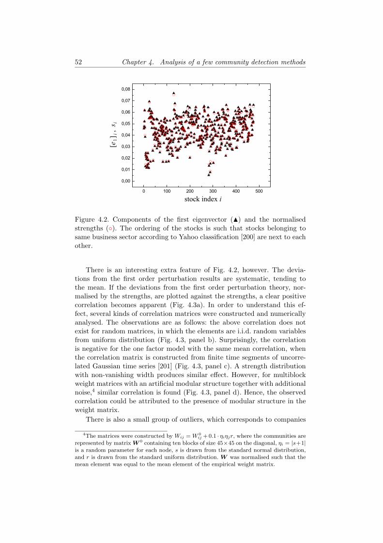
52 Chapter 4. Analysis of a few community detection methods
Figure 4.2. Components of the first eigenvector (N) and the normalisedstrengths (◦). The ordering of the stocks is such that stocks belonging tosame business sector according to Yahoo classification [200] are next to eachother.
There is an interesting extra feature of Fig. 4.2, however. The devia-tions from the first order perturbation results are systematic, tending tothe mean. If the deviations from the first order perturbation theory, nor-malised by the strengths, are plotted against the strengths, a clear positivecorrelation becomes apparent (Fig. 4.3a). In order to understand this ef-fect, several kinds of correlation matrices were constructed and numericallyanalysed. The observations are as follows: the above correlation does notexist for random matrices, in which the elements are i.i.d. random variablesfrom uniform distribution (Fig. 4.3, panel b). Surprisingly, the correlationis negative for the one factor model with the same mean correlation, whenthe correlation matrix is constructed from finite time segments of uncorre-lated Gaussian time series [201] (Fig. 4.3, panel c). A strength distributionwith non-vanishing width produces similar effect. However, for multiblockweight matrices with an artificial modular structure together with additionalnoise,4 similar correlation is found (Fig. 4.3, panel d). Hence, the observedcorrelation could be attributed to the presence of modular structure in theweight matrix.
There is also a small group of outliers, which corresponds to companies
4The matrices were constructed by Wij = W 0ij + 0.1 · ηiηjr, where the communities are
represented by matrix W 0 containing ten blocks of size 45×45 on the diagonal, ηi = |s+1|is a random parameter for each node, s is drawn from the standard normal distribution,and r is drawn from the standard uniform distribution. W was normalised such that themean element was equal to the mean element of the empirical weight matrix.
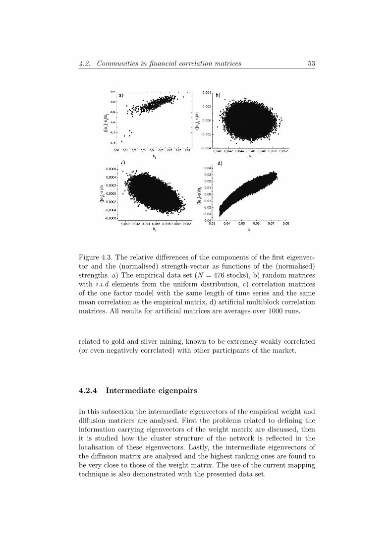
4.2. Communities in financial correlation matrices 53
Figure 4.3. The relative differences of the components of the first eigenvec-tor and the (normalised) strength-vector as functions of the (normalised)strengths. a) The empirical data set (N = 476 stocks), b) random matriceswith i.i.d elements from the uniform distribution, c) correlation matricesof the one factor model with the same length of time series and the samemean correlation as the empirical matrix, d) artificial multiblock correlationmatrices. All results for artificial matrices are averages over 1000 runs.
related to gold and silver mining, known to be extremely weakly correlated(or even negatively correlated) with other participants of the market.
4.2.4 Intermediate eigenpairs
In this subsection the intermediate eigenvectors of the empirical weight anddiffusion matrices are analysed. First the problems related to defining theinformation carrying eigenvectors of the weight matrix are discussed, thenit is studied how the cluster structure of the network is reflected in thelocalisation of these eigenvectors. Lastly, the intermediate eigenvectors ofthe diffusion matrix are analysed and the highest ranking ones are found tobe very close to those of the weight matrix. The use of the current mappingtechnique is also demonstrated with the presented data set.
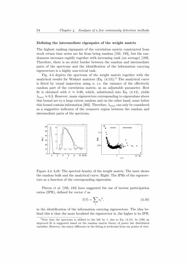
54 Chapter 4. Analysis of a few community detection methods
Defining the intermediate eigenpairs of the weight matrix
The highest ranking eigenpairs of the correlation matrix constructed fromstock return time series are far from being random [192, 193], but the ran-domness increases rapidly together with increasing rank (on average) [189].Therefore, there is no strict border between the random and intermediateparts of the spectrum and the identification of the information carryingeigenvectors is a highly non-trivial task.
Fig. 4.4 depicts the spectrum of the weight matrix together with theanalytical results for Wishart matrices (Eq. (4.13)).5 The analytical curveis fitted by visual inspection using σ, i.e. the variance of the effectivelyrandom part of the correlation matrix, as an adjustable parameter. Bestfit is obtained with σ ≈ 0.86, which, substituted into Eq. (4.14), yieldsλmax ≈ 0.3. However, many eigenvectors corresponding to eigenvalues abovethis bound are to a large extent random and on the other hand, some belowthis bound contain information [202]. Therefore, λmax can only be consideredas a suggestive indicator of the crossover region between the random andintermediate parts of the spectrum.
0 2 4 6 8 10 80 820
10
20
30
40
50
60
-0,8 -0,4 0,0 0,4 0,80
20
40
60
N(
)
1 10 82
0,01
0,1
IPR
+1
random intermediate
Figure 4.4. Left: The spectral density of the weight matrix. The inset showsthe random bulk and the analytical curve. Right: The IPRs of the eigenvec-tors as a function of the corresponding eigenvalue.
Plerou et al. [193, 194] have suggested the use of inverse participationratios (IPR), defined for vector ~v as
I(~v) =∑i
v 4i , (4.16)
in the identification of the information carrying eigenvectors. The idea be-hind this is that the more localised the eigenvector is, the higher is its IPR.
5Note that the spectrum is shifted to the left by 1, due to Eq. (4.15). In [199] animproved fit is suggested based on the random matrix theory of power law distributedvariables. However, the minor difference in the fitting is irrelevant from our points of view.
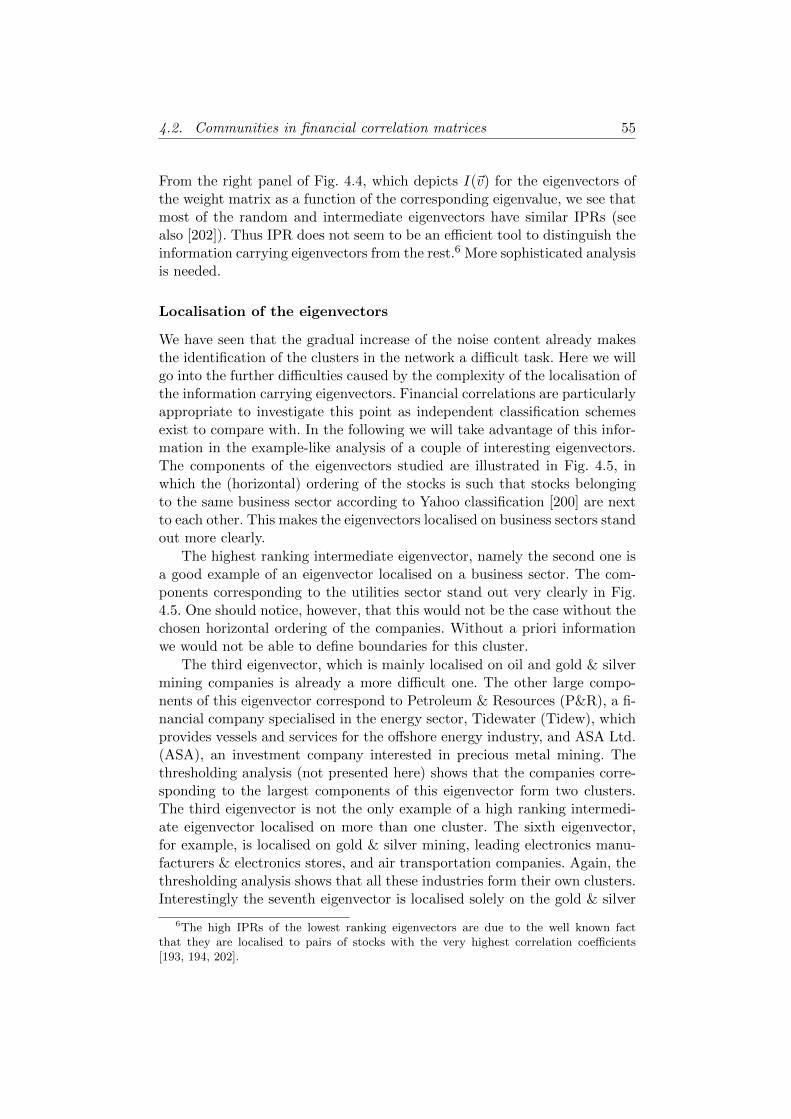
4.2. Communities in financial correlation matrices 55
From the right panel of Fig. 4.4, which depicts I(~v) for the eigenvectors ofthe weight matrix as a function of the corresponding eigenvalue, we see thatmost of the random and intermediate eigenvectors have similar IPRs (seealso [202]). Thus IPR does not seem to be an efficient tool to distinguish theinformation carrying eigenvectors from the rest.6 More sophisticated analysisis needed.
Localisation of the eigenvectors
We have seen that the gradual increase of the noise content already makesthe identification of the clusters in the network a difficult task. Here we willgo into the further difficulties caused by the complexity of the localisation ofthe information carrying eigenvectors. Financial correlations are particularlyappropriate to investigate this point as independent classification schemesexist to compare with. In the following we will take advantage of this infor-mation in the example-like analysis of a couple of interesting eigenvectors.The components of the eigenvectors studied are illustrated in Fig. 4.5, inwhich the (horizontal) ordering of the stocks is such that stocks belongingto the same business sector according to Yahoo classification [200] are nextto each other. This makes the eigenvectors localised on business sectors standout more clearly.
The highest ranking intermediate eigenvector, namely the second one isa good example of an eigenvector localised on a business sector. The com-ponents corresponding to the utilities sector stand out very clearly in Fig.4.5. One should notice, however, that this would not be the case without thechosen horizontal ordering of the companies. Without a priori informationwe would not be able to define boundaries for this cluster.
The third eigenvector, which is mainly localised on oil and gold & silvermining companies is already a more difficult one. The other large compo-nents of this eigenvector correspond to Petroleum & Resources (P&R), a fi-nancial company specialised in the energy sector, Tidewater (Tidew), whichprovides vessels and services for the offshore energy industry, and ASA Ltd.(ASA), an investment company interested in precious metal mining. Thethresholding analysis (not presented here) shows that the companies corre-sponding to the largest components of this eigenvector form two clusters.The third eigenvector is not the only example of a high ranking intermedi-ate eigenvector localised on more than one cluster. The sixth eigenvector,for example, is localised on gold & silver mining, leading electronics manu-facturers & electronics stores, and air transportation companies. Again, thethresholding analysis shows that all these industries form their own clusters.Interestingly the seventh eigenvector is localised solely on the gold & silver
6The high IPRs of the lowest ranking eigenvectors are due to the well known factthat they are localised to pairs of stocks with the very highest correlation coefficients[193, 194, 202].
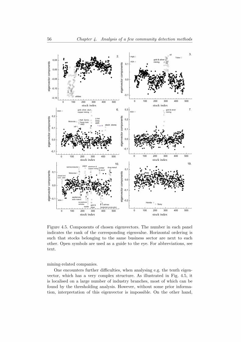
56 Chapter 4. Analysis of a few community detection methods
Figure 4.5. Components of chosen eigenvectors. The number in each panelindicates the rank of the corresponding eigenvalue. Horizontal ordering issuch that stocks belonging to the same business sector are next to eachother. Open symbols are used as a guide to the eye. For abbreviations, seetext.
mining-related companies.
One encounters further difficulties, when analysing e.g. the tenth eigen-vector, which has a very complex structure. As illustrated in Fig. 4.5, itis localised on a large number of industry branches, most of which can befound by the thresholding analysis. However, without some prior informa-tion, interpretation of this eigenvector is impossible. On the other hand,
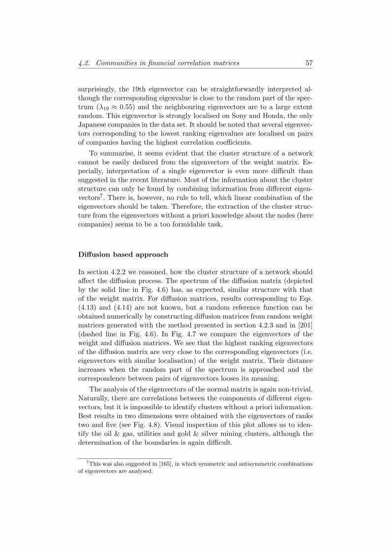
4.2. Communities in financial correlation matrices 57
surprisingly, the 19th eigenvector can be straightforwardly interpreted al-though the corresponding eigenvalue is close to the random part of the spec-trum (λ19 ≈ 0.55) and the neighbouring eigenvectors are to a large extentrandom. This eigenvector is strongly localised on Sony and Honda, the onlyJapanese companies in the data set. It should be noted that several eigenvec-tors corresponding to the lowest ranking eigenvalues are localised on pairsof companies having the highest correlation coefficients.
To summarise, it seems evident that the cluster structure of a networkcannot be easily deduced from the eigenvectors of the weight matrix. Es-pecially, interpretation of a single eigenvector is even more difficult thansuggested in the recent literature. Most of the information about the clusterstructure can only be found by combining information from different eigen-vectors7. There is, however, no rule to tell, which linear combination of theeigenvectors should be taken. Therefore, the extraction of the cluster struc-ture from the eigenvectors without a priori knowledge about the nodes (herecompanies) seems to be a too formidable task.
Diffusion based approach
In section 4.2.2 we reasoned, how the cluster structure of a network shouldaffect the diffusion process. The spectrum of the diffusion matrix (depictedby the solid line in Fig. 4.6) has, as expected, similar structure with thatof the weight matrix. For diffusion matrices, results corresponding to Eqs.(4.13) and (4.14) are not known, but a random reference function can beobtained numerically by constructing diffusion matrices from random weightmatrices generated with the method presented in section 4.2.3 and in [201](dashed line in Fig. 4.6). In Fig. 4.7 we compare the eigenvectors of theweight and diffusion matrices. We see that the highest ranking eigenvectorsof the diffusion matrix are very close to the corresponding eigenvectors (i.e.eigenvectors with similar localisation) of the weight matrix. Their distanceincreases when the random part of the spectrum is approached and thecorrespondence between pairs of eigenvectors looses its meaning.
The analysis of the eigenvectors of the normal matrix is again non-trivial.Naturally, there are correlations between the components of different eigen-vectors, but it is impossible to identify clusters without a priori information.Best results in two dimensions were obtained with the eigenvectors of rankstwo and five (see Fig. 4.8). Visual inspection of this plot allows us to iden-tify the oil & gas, utilities and gold & silver mining clusters, although thedetermination of the boundaries is again difficult.
7This was also suggested in [165], in which symmetric and antisymmetric combinationsof eigenvectors are analysed.

58 Chapter 4. Analysis of a few community detection methods
-1,05 -1,00 -0,95 -0,90 -0,851
10
N(
)
Figure 4.6. Spectral density of the diffusion matrix corresponding to thedataset (solid line), and the average spectral density over a system of 1000random references (dashed line). The trivial eigenvalue at 0 is not shown.
0 100 200 300 400 500
0,0
0,2
0,4
0,6
0,8
1,0
eWeD
eigenvector labels
Figure 4.7. Scalar products of the eigenvectors of the diffusion matrix andthe corresponding eigenvectors (i.e. eigenvectors with similar localisation)of the weight matrix. The eigenvectors of the diffusion matrix are orderedaccording to decreasing rank (x-axis).
4.2.5 Conclusions
It is well known that correlation matrices of stock prices have cluster struc-ture, which is reflected by the spectrum and the eigenvalues [165]. Here,I showed that the deviations from first order perturbation theory of theelements of the first eigenvector are positively correlated with the nodestrengths in an empirical network possessing a cluster structure. The positivecorrelation is absent for clusterless but otherwise similar artificial correlation
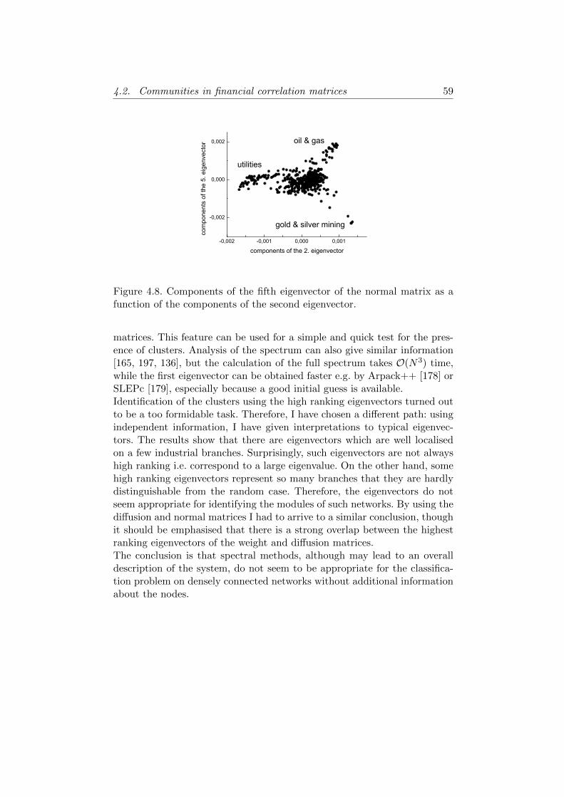
4.2. Communities in financial correlation matrices 59
-0,002 -0,001 0,000 0,001
-0,002
0,000
0,002
com
pone
nts
of th
e 5.
eig
enve
ctor
components of the 2. eigenvector
utilities
oil & gas
gold & silver mining
Figure 4.8. Components of the fifth eigenvector of the normal matrix as afunction of the components of the second eigenvector.
matrices. This feature can be used for a simple and quick test for the pres-ence of clusters. Analysis of the spectrum can also give similar information[165, 197, 136], but the calculation of the full spectrum takes O(N3) time,while the first eigenvector can be obtained faster e.g. by Arpack++ [178] orSLEPc [179], especially because a good initial guess is available.Identification of the clusters using the high ranking eigenvectors turned outto be a too formidable task. Therefore, I have chosen a different path: usingindependent information, I have given interpretations to typical eigenvec-tors. The results show that there are eigenvectors which are well localisedon a few industrial branches. Surprisingly, such eigenvectors are not alwayshigh ranking i.e. correspond to a large eigenvalue. On the other hand, somehigh ranking eigenvectors represent so many branches that they are hardlydistinguishable from the random case. Therefore, the eigenvectors do notseem appropriate for identifying the modules of such networks. By using thediffusion and normal matrices I had to arrive to a similar conclusion, thoughit should be emphasised that there is a strong overlap between the highestranking eigenvectors of the weight and diffusion matrices.The conclusion is that spectral methods, although may lead to an overalldescription of the system, do not seem to be appropriate for the classifica-tion problem on densely connected networks without additional informationabout the nodes.
60 Chapter 4. Analysis of a few community detection methods
4.3 Comparison of selected community detectionmethods on a large empirical network
Testing community detection methods is a problematic issue. Usually, testsare done on very small empirical networks, or on synthetic benchmarks incor-porating only a few features of real-world networks. Runs on large empiricalnetworks are lacking. The goal of this section is to start filling this gap.
Because the true community structure is unknown for empirical net-works, except really small ones, one cannot evaluate the result of a singlemethod in itself. Therefore, more methods are run on the same network,and their outputs are compared. The selection was aimed towards influen-tial methods which represent different underlying philosophies. Acceptablerunning time was also important, allowing only methods faster than O(N2).The Louvain method (LV) [62] (representing the modularity optimisationfamily), Infomap (IM) [98] and weighted Clique Percolation (wCP) [134]were chosen.
As the test network, a graph constructed from mobile phone calls wasused. Data are from a single European operator, covering 20% of the pop-ulation of its country. The records cover a period of 126 days. To ensureanonymity of customers, phone numbers have been replaced by surrogatekeys. Data from the same operator has been previously studied in [151, 59,166]. For this study, only voice calls were used, and only those that tookplace between customers of the operator in question. In addition edges wereexcluded where only one person had made calls to the other during thewhole period. Only the largest connected component is studied, which hasN = 4.9 × 10⁶ nodes and L = 10.9 × 10⁶ edges (mean degree 〈k〉 ≈ 4.44)8.The edges are weighted, edge weights are defined as sums of call durations(in seconds) between the two customers. The average weight is 〈w〉 ≈ 4634seconds. To sign that the community detection methods were applied to aweighted network, a “w” prefix will be put before their acronyms.
To evaluate the different methods, the results are compared in two ways:first at the level of single nodes, then on the scale of communities.
Two methods, wIM and wLV, are stochastic, they depend on the orderingof the nodes. Therefore, the stability of their results was tested9. They wererun 20 times, and the fraction of exactly matching communities among allthe 20 runs was calculated. It was found that on the weighted graph, for wIM(wLV) 92.5% (90.1%) of the communities were the same. The variation comesmostly from large communities. The high stability of wIM and wLV may bepartly explained by the fat-tailed distribution of call lengths in the mobilecall network [59]. An edge with a weight several orders of magnitude larger
8The largest connected component contains 92% of nodes and 98% of edges; the second-largest component has only 47 nodes.
9Appeared in the same paper as the results of this section, but found by anotherauthors.
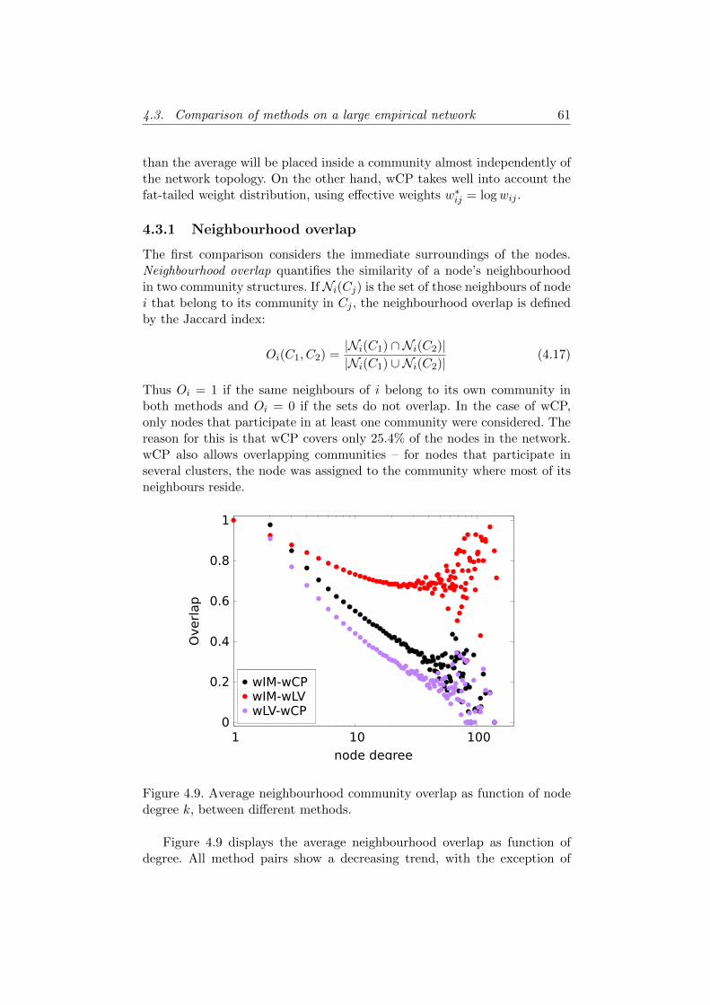
4.3. Comparison of methods on a large empirical network 61
than the average will be placed inside a community almost independently ofthe network topology. On the other hand, wCP takes well into account thefat-tailed weight distribution, using effective weights w∗ij = logwij .
4.3.1 Neighbourhood overlap
The first comparison considers the immediate surroundings of the nodes.Neighbourhood overlap quantifies the similarity of a node’s neighbourhoodin two community structures. If Ni(Cj) is the set of those neighbours of nodei that belong to its community in Cj , the neighbourhood overlap is definedby the Jaccard index:
Oi(C1, C2) =|Ni(C1) ∩Ni(C2)||Ni(C1) ∪Ni(C2)|
(4.17)
Thus Oi = 1 if the same neighbours of i belong to its own community inboth methods and Oi = 0 if the sets do not overlap. In the case of wCP,only nodes that participate in at least one community were considered. Thereason for this is that wCP covers only 25.4% of the nodes in the network.wCP also allows overlapping communities – for nodes that participate inseveral clusters, the node was assigned to the community where most of itsneighbours reside.
0
0.2
0.4
0.6
0.8
1
1 10 100
Overl
ap
node degree
wIM-wCP wIM-wLV wLV-wCP
Figure 4.9. Average neighbourhood community overlap as function of nodedegree k, between different methods.
Figure 4.9 displays the average neighbourhood overlap as function ofdegree. All method pairs show a decreasing trend, with the exception of
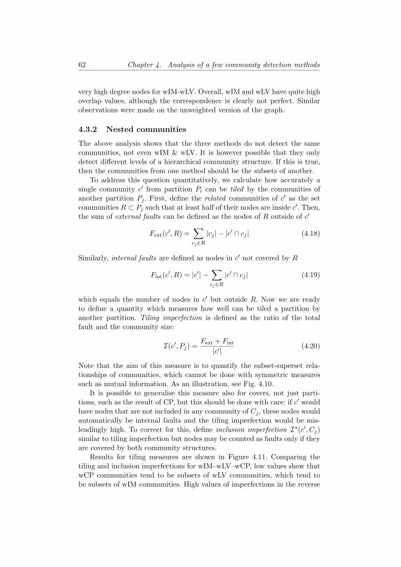
62 Chapter 4. Analysis of a few community detection methods
very high degree nodes for wIM-wLV. Overall, wIM and wLV have quite highoverlap values, although the correspondence is clearly not perfect. Similarobservations were made on the unweighted version of the graph.
4.3.2 Nested communities
The above analysis shows that the three methods do not detect the samecommunities, not even wIM & wLV. It is however possible that they onlydetect different levels of a hierarchical community structure. If this is true,then the communities from one method should be the subsets of another.
To address this question quantitatively, we calculate how accurately asingle community c′ from partition Pi can be tiled by the communities ofanother partition Pj . First, define the related communities of c′ as the setcommunities R ⊂ Pj such that at least half of their nodes are inside c′. Then,the sum of external faults can be defined as the nodes of R outside of c′
Fext(c′, R) =
∑cj∈R|cj | − |c′ ∩ cj | (4.18)
Similarly, internal faults are defined as nodes in c′ not covered by R
Fint(c′, R) = |c′| −
∑cj∈R|c′ ∩ cj | (4.19)
which equals the number of nodes in c′ but outside R. Now we are readyto define a quantity which measures how well can be tiled a partition byanother partition. Tiling imperfection is defined as the ratio of the totalfault and the community size:
I(c′, Pj) =Fext + Fint
|c′|(4.20)
Note that the aim of this measure is to quantify the subset-superset rela-tionships of communities, which cannot be done with symmetric measuressuch as mutual information. As an illustration, see Fig. 4.10.
It is possible to generalise this measure also for covers, not just parti-tions, such as the result of CP, but this should be done with care: if c′ wouldhave nodes that are not included in any community of Cj , these nodes wouldautomatically be internal faults and the tiling imperfection would be mis-leadingly high. To correct for this, define inclusion imperfection I∗(c′, Cj)similar to tiling imperfection but nodes may be counted as faults only if theyare covered by both community structures.
Results for tiling measures are shown in Figure 4.11. Comparing thetiling and inclusion imperfections for wIM–wLV–wCP, low values show thatwCP communities tend to be subsets of wLV communities, which tend tobe subsets of wIM communities. High values of imperfections in the reverse
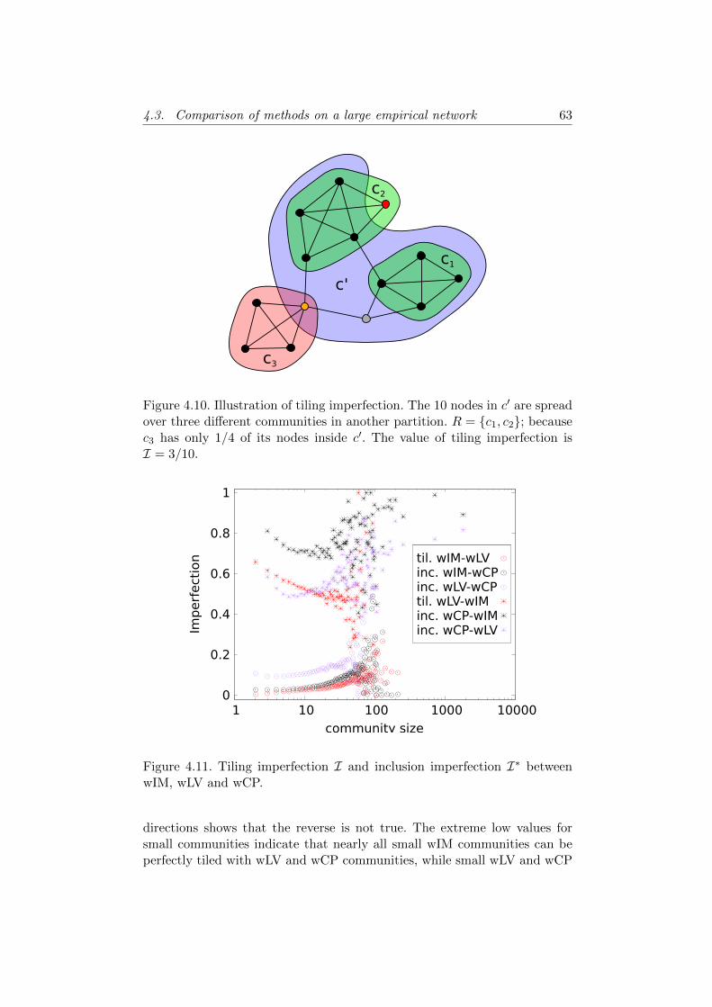
4.3. Comparison of methods on a large empirical network 63
c'
c1
c2
c3
Figure 4.10. Illustration of tiling imperfection. The 10 nodes in c′ are spreadover three different communities in another partition. R = {c1, c2}; becausec3 has only 1/4 of its nodes inside c′. The value of tiling imperfection isI = 3/10.
0
0.2
0.4
0.6
0.8
1
1 10 100 1000 10000
Imperf
ect
ion
community size
til. wIM-wLV inc. wIM-wCP inc. wLV-wCP til. wLV-wIM inc. wCP-wIM inc. wCP-wLV
Figure 4.11. Tiling imperfection I and inclusion imperfection I∗ betweenwIM, wLV and wCP.
directions shows that the reverse is not true. The extreme low values forsmall communities indicate that nearly all small wIM communities can beperfectly tiled with wLV and wCP communities, while small wLV and wCP
64 Chapter 4. Analysis of a few community detection methods
communities can rarely be tiled with wIM communities.Hierarchical relations can be obtained also for the unweighted version of
the network; however, in that case the IM and LV methods’ output is lessstable (in 20 runs, 13.2% and 36.7% of the communities were exact matches,respectively).
4.3.3 Conclusions
As we saw, the communities produced by three different methods on a largeempirical network corresponded surprisingly well to the different levels of asingle hierarchical (nested, multilevel) community structure. There are im-portant remarks, though. The weighted Clique Percolation method coveredonly 25.4% of the graph, so similarity of wCP holds only on this subset.Furthermore, it is known10 that a large portion of the graph is tree-like(very far from the picture of a good community), and this tree-like part isclustered into several small communities. The concordance of the weightedInfomap and Louvain methods for small communities may be increased bythem. Strong weights may also cause convergence. For larger communities,agreement between the methods decreases, but still surprisingly strong.
10Appeared in the same paper as the matter of this section, but found by anotherauthors.
Chapter 5
Criterions for locally densesubgraphs
After being the subject of active research for several years, it is getting clearthat the following stages appear during community detection:
1 defining the term “community”;
2 finding the objects corresponding to the definition;
3 determining the significance of the found communities.
Although community detection attracted a lot of attention in the last decade,there is still no real definition of the term “community”. This is the funda-mental reason for the proliferation of methods, and for our inability to judgethe output of them. Of course, the latter fact strongly limits the possibleapplications. The current chapter contributes to this issue. First, a list ofrequired properties are established, along with the review of the currentmethods, then an implementation (a new detection method) is presentedalong with test results.
5.1 Local criteria for communities
A fundamental problem of community detection is to define the term “com-munity”. There are different approaches to this question. One is the algorith-mic approach, giving a computational procedure for finding clusters. Thisnaturally incorporates a mathematically precise definition, although differ-ent algorithms usually result in diverse definitions, and there is no theoreticalframework currently to help their differentiation. Another possibility is topresent a general concept, on which a precise definition can be based. In thischapter, the latter approach is taken, although an algorithmic realisation isalso presented.
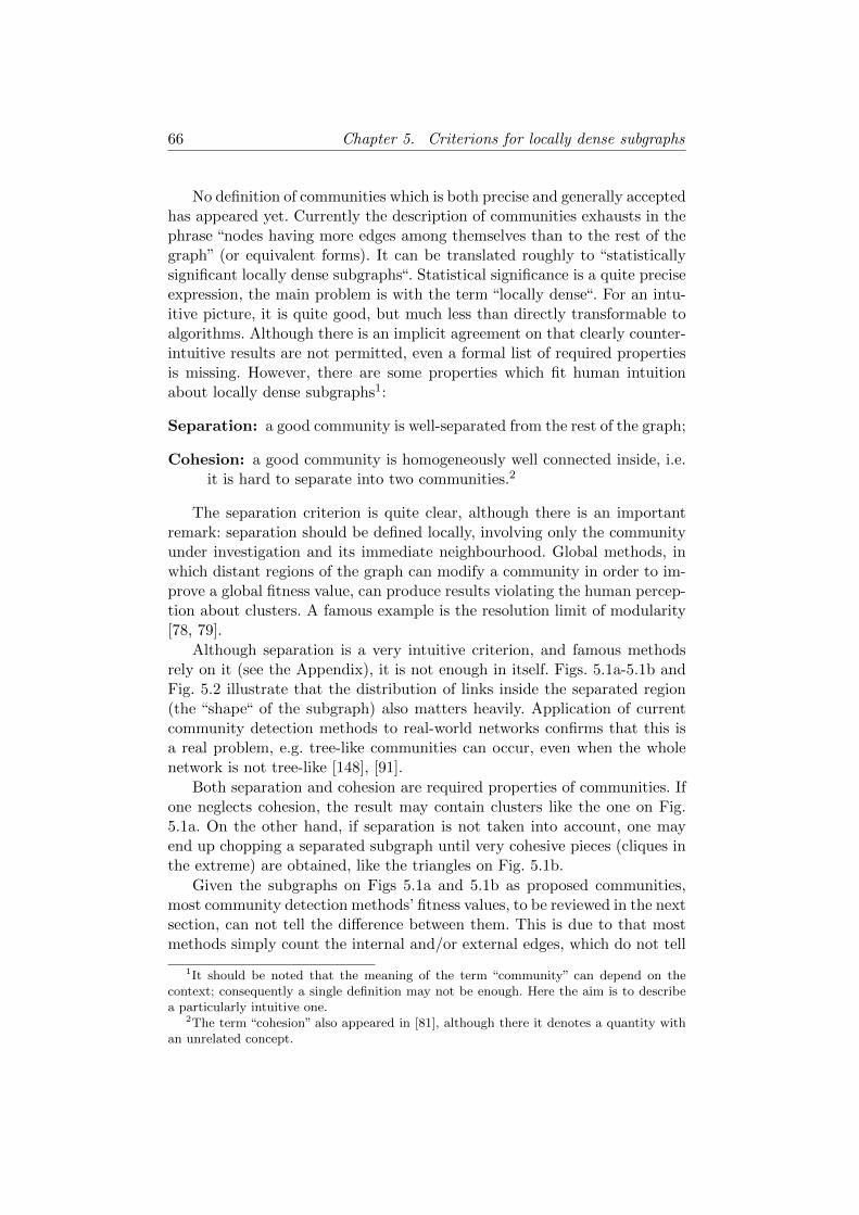
66 Chapter 5. Criterions for locally dense subgraphs
No definition of communities which is both precise and generally acceptedhas appeared yet. Currently the description of communities exhausts in thephrase “nodes having more edges among themselves than to the rest of thegraph” (or equivalent forms). It can be translated roughly to “statisticallysignificant locally dense subgraphs“. Statistical significance is a quite preciseexpression, the main problem is with the term “locally dense“. For an intu-itive picture, it is quite good, but much less than directly transformable toalgorithms. Although there is an implicit agreement on that clearly counter-intuitive results are not permitted, even a formal list of required propertiesis missing. However, there are some properties which fit human intuitionabout locally dense subgraphs1:
Separation: a good community is well-separated from the rest of the graph;
Cohesion: a good community is homogeneously well connected inside, i.e.it is hard to separate into two communities.2
The separation criterion is quite clear, although there is an importantremark: separation should be defined locally, involving only the communityunder investigation and its immediate neighbourhood. Global methods, inwhich distant regions of the graph can modify a community in order to im-prove a global fitness value, can produce results violating the human percep-tion about clusters. A famous example is the resolution limit of modularity[78, 79].
Although separation is a very intuitive criterion, and famous methodsrely on it (see the Appendix), it is not enough in itself. Figs. 5.1a-5.1b andFig. 5.2 illustrate that the distribution of links inside the separated region(the “shape“ of the subgraph) also matters heavily. Application of currentcommunity detection methods to real-world networks confirms that this isa real problem, e.g. tree-like communities can occur, even when the wholenetwork is not tree-like [148], [91].
Both separation and cohesion are required properties of communities. Ifone neglects cohesion, the result may contain clusters like the one on Fig.5.1a. On the other hand, if separation is not taken into account, one mayend up chopping a separated subgraph until very cohesive pieces (cliques inthe extreme) are obtained, like the triangles on Fig. 5.1b.
Given the subgraphs on Figs 5.1a and 5.1b as proposed communities,most community detection methods’ fitness values, to be reviewed in the nextsection, can not tell the difference between them. This is due to that mostmethods simply count the internal and/or external edges, which do not tell
1It should be noted that the meaning of the term “community” can depend on thecontext; consequently a single definition may not be enough. Here the aim is to describea particularly intuitive one.
2The term “cohesion” also appeared in [81], although there it denotes a quantity withan unrelated concept.
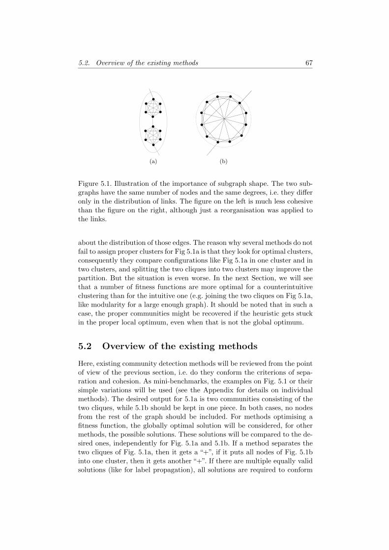
5.2. Overview of the existing methods 67
(a) (b)
Figure 5.1. Illustration of the importance of subgraph shape. The two sub-graphs have the same number of nodes and the same degrees, i.e. they differonly in the distribution of links. The figure on the left is much less cohesivethan the figure on the right, although just a reorganisation was applied tothe links.
about the distribution of those edges. The reason why several methods do notfail to assign proper clusters for Fig 5.1a is that they look for optimal clusters,consequently they compare configurations like Fig 5.1a in one cluster and intwo clusters, and splitting the two cliques into two clusters may improve thepartition. But the situation is even worse. In the next Section, we will seethat a number of fitness functions are more optimal for a counterintuitiveclustering than for the intuitive one (e.g. joining the two cliques on Fig 5.1a,like modularity for a large enough graph). It should be noted that in such acase, the proper communities might be recovered if the heuristic gets stuckin the proper local optimum, even when that is not the global optimum.
5.2 Overview of the existing methods
Here, existing community detection methods will be reviewed from the pointof view of the previous section, i.e. do they conform the criterions of sepa-ration and cohesion. As mini-benchmarks, the examples on Fig. 5.1 or theirsimple variations will be used (see the Appendix for details on individualmethods). The desired output for 5.1a is two communities consisting of thetwo cliques, while 5.1b should be kept in one piece. In both cases, no nodesfrom the rest of the graph should be included. For methods optimising afitness function, the globally optimal solution will be considered, for othermethods, the possible solutions. These solutions will be compared to the de-sired ones, independently for Fig. 5.1a and 5.1b. If a method separates thetwo cliques of Fig. 5.1a, then it gets a “+”, if it puts all nodes of Fig. 5.1binto one cluster, then it gets another “+”. If there are multiple equally validsolutions (like for label propagation), all solutions are required to conform
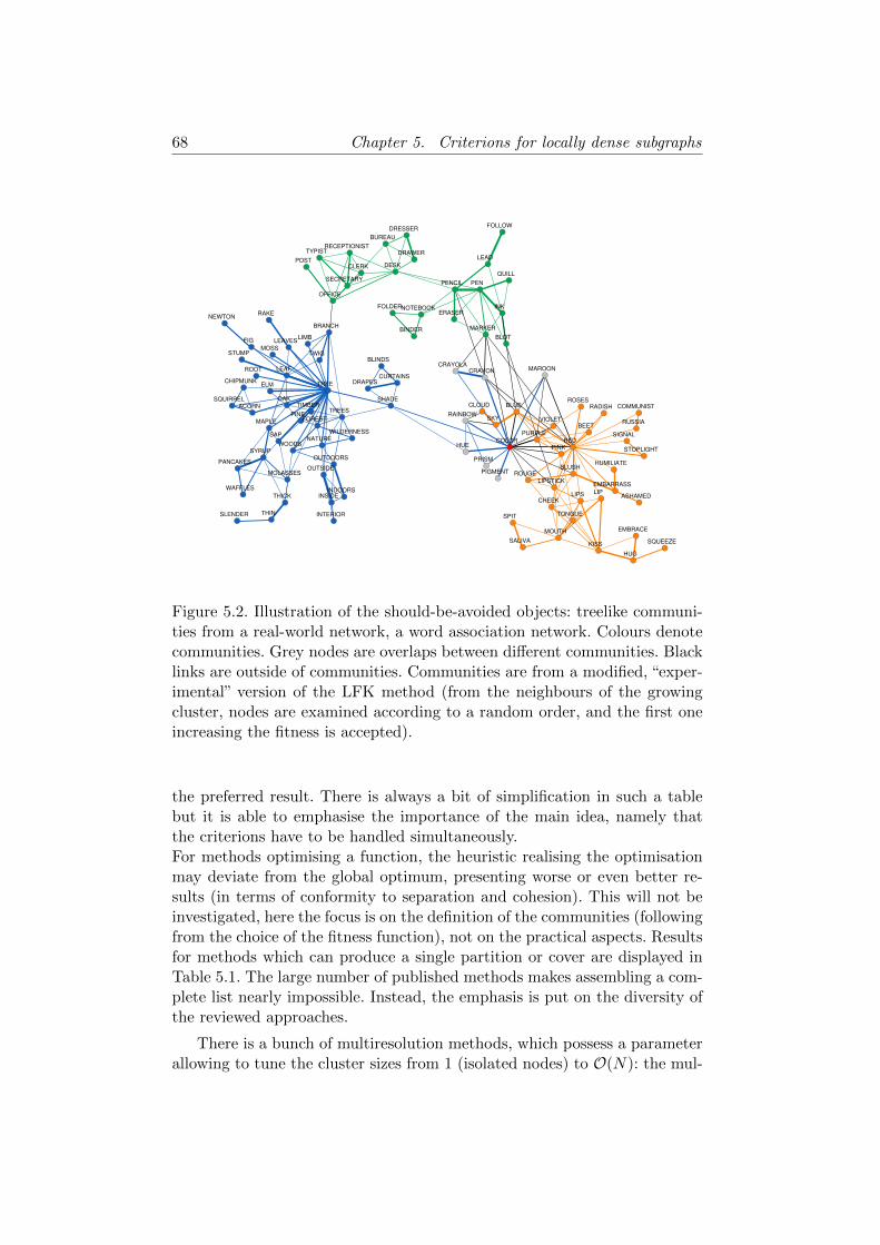
68 Chapter 5. Criterions for locally dense subgraphs
OFFICE
RECEPTIONIST
POSTDRAWER
DRESSER
DESK
TYPIST
SECRETARY
CLERK
BUREAU
LIMB
BRANCH
TWIGMOSS
RAKE
STUMP
NEWTON
LEAVESFIG
ROOT LEAF
CHIPMUNKELM
ACORNSQUIRREL OAK
TIMBER
PENCIL
NOTEBOOK
PEN
ERASER
BINDER
FOLDER
MARKER
RAINBOW
BLOT
LEAD
FOLLOW
QUILL
INK
CRAYOLA
THIN
PANCAKES
MOLASSES
THICK
WAFFLES
SLENDER
SYRUPWOODS
MAPLEPINE
FOREST
SAP WILDERNESS
TREES
NATURE
OUTDOORS
INSIDEINDOORS
INTERIOR
OUTSIDE
CURTAINS
SHADE
DRAPESTREE
BLINDS
RED
STOPLIGHT
RADISH COMMUNISTROSES
SIGNAL
VIOLET
PINK
RUSSIABEET
LIP
BLUSH
CHEEK
LIPSTICK
HUMILIATE
EMBARRASS
LIPS ASHAMED
TONGUE
SALIVAKISS
SPIT
MOUTH
HUG
EMBRACE
SQUEEZE
ROUGE
PURPLE
MAROON
BLUE
COLOR
CRAYON
PIGMENT
CLOUD
HUE
PRISM
SKY
Figure 5.2. Illustration of the should-be-avoided objects: treelike communi-ties from a real-world network, a word association network. Colours denotecommunities. Grey nodes are overlaps between different communities. Blacklinks are outside of communities. Communities are from a modified, “exper-imental” version of the LFK method (from the neighbours of the growingcluster, nodes are examined according to a random order, and the first oneincreasing the fitness is accepted).
the preferred result. There is always a bit of simplification in such a tablebut it is able to emphasise the importance of the main idea, namely thatthe criterions have to be handled simultaneously.For methods optimising a function, the heuristic realising the optimisationmay deviate from the global optimum, presenting worse or even better re-sults (in terms of conformity to separation and cohesion). This will not beinvestigated, here the focus is on the definition of the communities (followingfrom the choice of the fitness function), not on the practical aspects. Resultsfor methods which can produce a single partition or cover are displayed inTable 5.1. The large number of published methods makes assembling a com-plete list nearly impossible. Instead, the emphasis is put on the diversity ofthe reviewed approaches.
There is a bunch of multiresolution methods, which possess a parameterallowing to tune the cluster sizes from 1 (isolated nodes) to O(N): the mul-
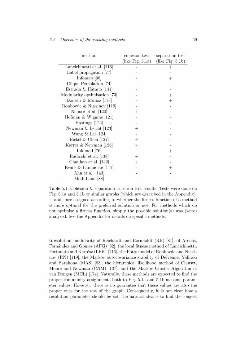
5.2. Overview of the existing methods 69
method cohesion test separation test(like Fig. 5.1a) (like Fig. 5.1b)
Lancichinetti et al. [116] - +Label propagation [77] - -
Infomap [98] - +Clique Percolation [74] - -Estrada & Hatano [141] - -
Modularity optimisation [73] - +Donetti & Munoz [173] - +
Ronhovde & Nussinov [119] - -Nepusz et al. [120] + -
Hofman & Wiggins [121] - -Hastings [122] - -
Newman & Leicht [123] + -Wang & Lai [124] + -
Bickel & Chen [127] + -Karrer & Newman [126] + -
Infomod [76] - +Radicchi et al. [138] + -Chauhan et al. [142] + -
Evans & Lambiotte [117] - +Ahn et al. [143] - -ModuLand [88] - -
Table 5.1. Cohesion & separation criterion test results. Tests were done onFig. 5.1a and 5.1b or similar graphs (which are described in the Appendix).+ and - are assigned according to whether the fitness function of a methodis more optimal for the preferred solution or not. For methods which donot optimise a fitness function, simply the possible solution(s) was (were)analysed. See the Appendix for details on specific methods.
tiresolution modularity of Reichardt and Bornholdt (RB) [81], of Arenas,Fernandez and Gomez (AFG) [82], the local fitness method of Lancichinetti,Fortunato and Kertesz (LFK) [116], the Potts model of Ronhovde and Nussi-nov (RN) [119], the Markov autocovariance stability of Delvenne, Yalirakiand Barahona (MAS) [83], the hierarchical likelihood method of Clauset,Moore and Newman (CNM) [137], and the Markov Cluster Algorithm ofvan Dongen (MCL) [174]. Naturally, these methods are expected to find theproper community assignments both to Fig. 5.1a and 5.1b at some param-eter values. However, there is no guarantee that these values are also theproper ones for the rest of the graph. Consequently, it is not clear how aresolution parameter should be set: the natural idea is to find the longest
70 Chapter 5. Criterions for locally dense subgraphs
interval of the resolution parameter value in which the community structuredoes not change, but when the optimal parameter value is different for dif-ferent regions in the graph, the longest stable interval not necessarily reflectsthe optimal communities.Furthermore, the fitness values do not help us to tell good clusters from badones, like Fig. 5.1a from Fig. 5.1b. For most multiresolution methods (RB,AFG, LFK, RN), it is very easy to see that the fitnesses of two clusters arethe same given that all nodes has the same in- and outdegrees, indepen-dently of the shape of the clusters. Note that it is also true for most singleresolution methods. For MAS it is not trivial. Therefore, empirical tests wereconducted to check it. According to them, Fig. 5.1a was found empiricallyto be at least as good as 5.1b3. Finally, regarding MCL and CNM, theyhave no fitness function4, the only accessible quantity about the communitystructure is the parameter interval in which it is stable.
Finally, there are hierarchical methods, which look for series of smallerand smaller (or larger and larger) clusters hierarchically embedded into theprevious ones. Similarly to multiresolution methods, they are expected tocontain good clusters in the outputted hierarchy. However, when looking ata graph having a simple one-level community structure, the question how toselect the proper levels of the outputted hierarchy arises. The easiest wayis to use the lowest level communities. Unfortunately, it is not a reliableprocedure, as the lowest-level clusters may be just parts of the communitiesof the optimal partition or cover (see the Appendix for details). A second ideacan be to assign significance scores to the communities on different levels, inthe spirit of [93]. Although this approach might reliably qualify the foundcommunities, a new version of statistical significance taking into account theinternal cohesion is required. Furthermore, one should be very careful not toimpose unnecessary constraints, like prohibiting overlaps, when constructinga hierarchical method.
A further question is whether a method provides information about theshape of the found communities or not. Recent analysis of real-world net-works highlights the relevance of this issue [148], [91]. Several methods arebased on simply counting the internal and/or external edges, or degreesat most: LFK, Label propagation, Infomap, modularity optimisation (andequivalents), Hofman & Wiggins, Hastings, Ronhovde & Nussinov, Newman& Leicht, Wang & Lai, Bickel & Chen, Karrer & Newman, Infomod, Ahnet al., OSLOM. Consequently, they do not see any difference in the distri-bution of the links, e.g. Fig 5.1a and 5.1b get the same fitness values. Only
3In this case, only 1 link to the rest of the graph was used. Rest of the graph, representedby a single node having self-loops, was assigned 118 edges inside, resulting in a total ofL = 150 edges. Stability values were calculated from 0.01 to 100, the step size being 0.01below 1.0 and 1 above.
4CNM does have a fitness function, but it corresponds to a full hierarchical dendrogram,not to any partitions obtained by cutting the dendrogram at some point

5.3. Community detection in a two dimensional parameter space 71
Clique Percolation and Radicchi et al.’s5 method have some very limitedrequirement about cohesion built in the definition of communities.
The conclusion is that none of the reviewed methods is able to success-fully apply both the separation and the cohesion criterions. They susceptibleeither to glue together well-separated subgraphs or to overpartition a cohe-sive subgraph. Future network designs should consider cohesion as well asseparation.
5.3 Community detection in a two dimensional pa-rameter space
In this section, a new method for community detection is introduced. Itsmain goal is to present a method which takes into account both criterionsdefined in Sec. 5.1. First, a composite fitness will be constructed which takesinto account the separation and cohesion criterions. Then, a heuristic opti-misation procedure for the composite fitness will be described, which findslocally dense subgraphs on all scales, and also able to recover hierarchicalstructures.
5.3.1 Implementing the criterions
For the separation criterion, the following function will be applied
fCS =KCin
KCin +KC
out
(5.1)
where C is a subgraph, Kin and Kout are the sums of in-community andout-community degrees, respectively. This is the fitness of LFK [116], withthe multiresolution parameter being set to one. For detecting hierarchicalstructures, a different solution will be described. Eq. 5.1 clearly focuses onthe external separation of the clusters, therefore it is suitable as an imple-mentation of the first criterion of the communities.
For the internal cohesion criterion, a possible solution is to consider thesecond eigenvalue of the Laplacian matrix of the community. The Laplacianof a graph is the matrix L = A −D, where A is the adjacency (or weight)matrix, Aij being 1 if there is a link between nodes i and j (Wij a real numberas the weight of the link), and D = diag(ki) is a diagonal matrix containingcontaining each node’s sum of links (weights). Its largest eigenvalue is always0 (corresponding to the trivial eigenvector (1, 1, . . . , 1)). The multiplicity ofthe largest eigenvalue equals to the number of connected components in thegraph. This gives the hint that if two distinct graphs are got connected by asingle (weak) link, the Laplacian gets only a slight perturbation (compared to
5If the stopping criterion of their heuristic is considered as part of the definition.
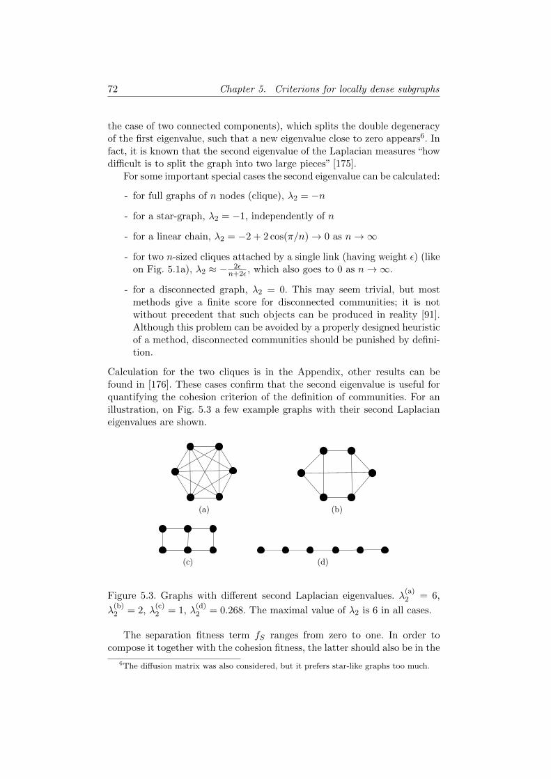
72 Chapter 5. Criterions for locally dense subgraphs
the case of two connected components), which splits the double degeneracyof the first eigenvalue, such that a new eigenvalue close to zero appears6. Infact, it is known that the second eigenvalue of the Laplacian measures “howdifficult is to split the graph into two large pieces” [175].
For some important special cases the second eigenvalue can be calculated:
- for full graphs of n nodes (clique), λ2 = −n
- for a star-graph, λ2 = −1, independently of n
- for a linear chain, λ2 = −2 + 2 cos(π/n)→ 0 as n→∞
- for two n-sized cliques attached by a single link (having weight ε) (likeon Fig. 5.1a), λ2 ≈ − 2ε
n+2ε , which also goes to 0 as n→∞.
- for a disconnected graph, λ2 = 0. This may seem trivial, but mostmethods give a finite score for disconnected communities; it is notwithout precedent that such objects can be produced in reality [91].Although this problem can be avoided by a properly designed heuristicof a method, disconnected communities should be punished by defini-tion.
Calculation for the two cliques is in the Appendix, other results can befound in [176]. These cases confirm that the second eigenvalue is useful forquantifying the cohesion criterion of the definition of communities. For anillustration, on Fig. 5.3 a few example graphs with their second Laplacianeigenvalues are shown.
(a) (b)
(c) (d)
Figure 5.3. Graphs with different second Laplacian eigenvalues. λ(a)2 = 6,
λ(b)2 = 2, λ
(c)2 = 1, λ
(d)2 = 0.268. The maximal value of λ2 is 6 in all cases.
The separation fitness term fS ranges from zero to one. In order tocompose it together with the cohesion fitness, the latter should also be in the
6The diffusion matrix was also considered, but it prefers star-like graphs too much.
5.3. Community detection in a two dimensional parameter space 73
interval [0, 1]. Therefore, λ2 needs some transformations before applicationas fitness.As can be seen from the above examples, for the worst cases |λ2| is of theorder of 1/n, therefore the lowest point of the |λ2|-scale will be set to 1/n.The highest point is trivially given by n. It is reasonable to assume thatmost subgraphs have |λ2| = o(|C|). Furthermore, several subgraphs canhave worse internal cohesion than the star graph, thus having |λ2| ∈ [0, 1].To take into account these effect, log |λ2| will be more useful than λ2. So, inorder to obtain a quantity between 0 and 1, the minimum will be subtractedand divided by the maximum,
fCC =log |λ2| − log 1/|C|log |C| − log 1/|C|
=1
2+
1
2
log |λ2|log |C|
, if |C| > 1
= 0 if |C| = 1
(5.2)
where |C| is the number of nodes in the community. The above measurehappens to be 0.5 if λ2 is 1, e.g. for the star-graph. I wish to emphasise thateq. 5.2 is only one possible proposition for taking into account the internalcohesion, although a promising one – better measures may exist. The sameis true for the choice of fS .
The cohesion fitness fCC opens the way for constructing tests assessingthe performance of community detection methods regarding the cohesion ofthe found communities. One may generate a graph with built-in communi-ties which separation is controlled, like in the LFR benchmark [102], thenrandomly select pairs of clusters and increase the interconnection betweenthe two members of each pairs to some predefined value, finally calculatingfCC of the pairs. Running the detection method and measuring the ratio ofpairs not split as a function of fCC may indicate how strongly focuses themethod on cohesion.
The next question is how to combine fCseparation and fCcohesion. Thinking
in a two dimensional space of fCS and fCC , a natural approach is to get asfar from the point (0, 0) as possible. This implies
fC =√
(fCS )2 + (fCC )2 (5.3)
so the fitness is the euclidean distance from (0, 0). Again, this is just onepossibility, better combinations may exist. E.g. the relative weight of fSand fC may be adjusted in a more well-grounded way. However, eq. 5.3is able to pass the test raised by Fig. 5.1: for Fig. 5.1a, λ2cliques
2 = 0.258,
f2cliquesC = 0.228, f2cliques = 0.995 while for a single clique λ1clique
2 = 6,
f1cliqueC = 1, f1clique = 1.371. For Fig. 5.1b, λ12nodes
2 = 3.268, f12nodesC =
0.738, f12nodes = 1.218, and for the best subgraph, a triangle, λtriangle2 = 3,
f triangleC = 1, f triangle = 1.077.
74 Chapter 5. Criterions for locally dense subgraphs
Beyond enabling one to decide whether a given subgraph is a communityor not (by requiring local optimality), the above definition makes it possi-ble to assess how good community it is. This is also possible with anotherdefinitions, e.g. by using the modularity function, but here, communitiesare placed on a 2-dimensional space instead of 1 dimension. This gives riseto an interesting possibility for characterising the communities, like “verycohesive but densely connected outwards” or “well-separated but poorly in-terconnected”. Considering Fig. 5.1a, one may think that the latter is notreally a community. But for large subgraphs, it may make sense to considera well-separated subgraph as a community, as common sense says that largecommunities should be looser than small ones.
5.3.2 Community detection in reality
In this subsection, the details of practical implementation of the new methodare discussed. Most importantly, in order to actually find the communities,a heuristic carrying out the optimisation of eq. 5.3 is needed. Furthermore,there is a second problem of detecting communities hierarchically embeddedinto each other. These two questions will be answered by a common solution.
The heuristic is based on the one of the LFK method [116]. Among itsdetails, the LFK heuristic contains a tunable parameter (denoted as α),which is claimed to be able to recover communities at different hierarchicallevels. Lowering this parameter α results in increased community sizes. Hier-archical levels are supposed to be stable against the variation of α, so thereshould be long intervals for α for which the communities do not change.However, large graphs may lack long stable intervals, as some changes occuraround any parameter value (data not shown). Therefore, a new method forinvestigating hierarchical structure is needed. I dropped the idea of usingthreshold values of α, corresponding to community structures at differentscales, which should be simultaneously valid for all communities, and I willtreat each community separately.
Similarly to [116], each community is grown from a seed node. It is im-portant to note that each seed node can result in a series of (successivelylarger) communities. Growth consists of successively including the neigh-bouring node which increases most the fitness defined by eq. 5.3. Whenthere is no neighbouring node which inclusion can improve the fitness, thestage of node removal begins. Here, the fitness of the cluster is tried to beimproved by excluding nodes from it (with the exception of the seed node,which is not permitted to be excluded). It finishes when no further removalcan improve the fitness. Then, growth begins again, if possible. The grow-shrink cycle is iterated, as long as the fitness can be improved. When noimprovement is possible (there is a local optimum of the fitness), the actuallist of nodes is registered as a valid community. After that, the algorithmtries to find a larger community, which contains the current one. This way,
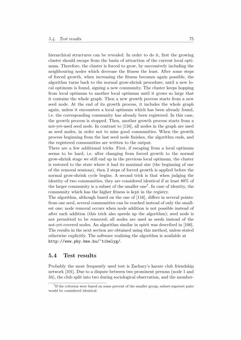
5.4. Test results 75
hierarchical structures can be revealed. In order to do it, first the growingcluster should escape from the basin of attraction of the current local opti-mum. Therefore, the cluster is forced to grow, by successively including theneighbouring nodes which decrease the fitness the least. After some stepsof forced growth, when increasing the fitness becomes again possible, thealgorithm turns back to the normal grow-shrink procedure, until a new lo-cal optimum is found, signing a new community. The cluster keeps hoppingfrom local optimum to another local optimum until it grows so large thatit contains the whole graph. Then a new growth process starts from a newseed node. At the end of its growth process, it includes the whole graphagain, unless it encounters a local optimum which has been already found,i.e. the corresponding community has already been registered. In this case,the growth process is stopped. Then, another growth process starts from anot-yet-used seed node. In contrast to [116], all nodes in the graph are usedas seed nodes, in order not to miss good communities. When the growthprocess beginning from the last seed node finishes, the algorithm ends, andthe registered communities are written to the output.There are a few additional tricks. First, if escaping from a local optimumseems to be hard, i.e. after changing from forced growth to the normalgrow-shrink stage we still end up in the previous local optimum, the clusteris restored to the state where it had its maximal size (the beginning of oneof the removal sessions), then 2 steps of forced growth is applied before thenormal grow-shrink cycle begins. A second trick is that when judging theidentity of two communities, they are considered identical if at least 80% ofthe larger community is a subset of the smaller one7. In case of identity, thecommunity which has the higher fitness is kept in the registry.The algorithm, although based on the one of [116], differs in several points:from one seed, several communities can be reached instead of only the small-est one; node removal occurs when node addition is not possible instead ofafter each addition (this trick also speeds up the algorithm); seed node isnot permitted to be removed; all nodes are used as seeds instead of thenot-yet-covered nodes. An algorithm similar in spirit was described in [100].The results in the next section are obtained using this method, unless statedotherwise explicitly. The software realising the algorithm is available athttp://www.phy.bme.hu/~tibelyg/.
5.4 Test results
Probably the most frequently used test is Zachary’s karate club friendshipnetwork [101]. Due to a dispute between two prominent persons (node 1 and34), the club split into two during sociological observation, and the member-
7If the criterion were based on some percent of the smaller group, subset-superset pairswould be considered identical.
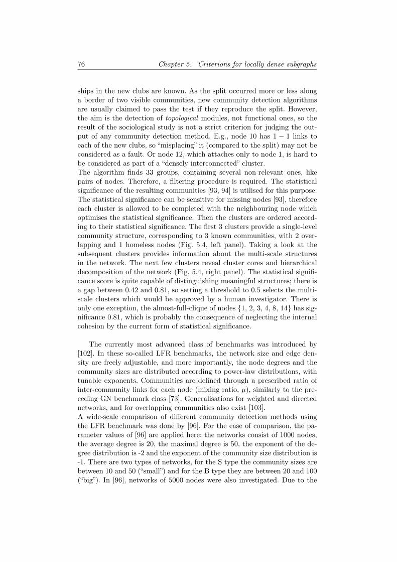
76 Chapter 5. Criterions for locally dense subgraphs
ships in the new clubs are known. As the split occurred more or less alonga border of two visible communities, new community detection algorithmsare usually claimed to pass the test if they reproduce the split. However,the aim is the detection of topological modules, not functional ones, so theresult of the sociological study is not a strict criterion for judging the out-put of any community detection method. E.g., node 10 has 1 − 1 links toeach of the new clubs, so “misplacing” it (compared to the split) may not beconsidered as a fault. Or node 12, which attaches only to node 1, is hard tobe considered as part of a “densely interconnected” cluster.The algorithm finds 33 groups, containing several non-relevant ones, likepairs of nodes. Therefore, a filtering procedure is required. The statisticalsignificance of the resulting communities [93, 94] is utilised for this purpose.The statistical significance can be sensitive for missing nodes [93], thereforeeach cluster is allowed to be completed with the neighbouring node whichoptimises the statistical significance. Then the clusters are ordered accord-ing to their statistical significance. The first 3 clusters provide a single-levelcommunity structure, corresponding to 3 known communities, with 2 over-lapping and 1 homeless nodes (Fig. 5.4, left panel). Taking a look at thesubsequent clusters provides information about the multi-scale structuresin the network. The next few clusters reveal cluster cores and hierarchicaldecomposition of the network (Fig. 5.4, right panel). The statistical signifi-cance score is quite capable of distinguishing meaningful structures; there isa gap between 0.42 and 0.81, so setting a threshold to 0.5 selects the multi-scale clusters which would be approved by a human investigator. There isonly one exception, the almost-full-clique of nodes {1, 2, 3, 4, 8, 14} has sig-nificance 0.81, which is probably the consequence of neglecting the internalcohesion by the current form of statistical significance.
The currently most advanced class of benchmarks was introduced by[102]. In these so-called LFR benchmarks, the network size and edge den-sity are freely adjustable, and more importantly, the node degrees and thecommunity sizes are distributed according to power-law distributions, withtunable exponents. Communities are defined through a prescribed ratio ofinter-community links for each node (mixing ratio, µ), similarly to the pre-ceding GN benchmark class [73]. Generalisations for weighted and directednetworks, and for overlapping communities also exist [103].A wide-scale comparison of different community detection methods usingthe LFR benchmark was done by [96]. For the ease of comparison, the pa-rameter values of [96] are applied here: the networks consist of 1000 nodes,the average degree is 20, the maximal degree is 50, the exponent of the de-gree distribution is -2 and the exponent of the community size distribution is-1. There are two types of networks, for the S type the community sizes arebetween 10 and 50 (“small”) and for the B type they are between 20 and 100(“big”). In [96], networks of 5000 nodes were also investigated. Due to the
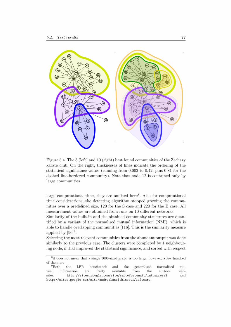
5.4. Test results 77
Figure 5.4. The 3 (left) and 10 (right) best found communities of the Zacharykarate club. On the right, thicknesses of lines indicate the ordering of thestatistical significance values (running from 0.002 to 0.42, plus 0.81 for thedashed line-bordered community). Note that node 12 is contained only bylarge communities.
large computational time, they are omitted here8. Also for computationaltime considerations, the detecting algorithm stopped growing the commu-nities over a predefined size, 120 for the S case and 220 for the B case. Allmeasurement values are obtained from runs on 10 different networks.Similarity of the built-in and the obtained community structures are quan-tified by a variant of the normalised mutual information (NMI), which isable to handle overlapping communities [116]. This is the similarity measureapplied by [96]9.Selecting the most relevant communities from the abundant output was donesimilarly to the previous case. The clusters were completed by 1 neighbour-ing node, if that improved the statistical significance, and sorted with respect
8it does not mean that a single 5000-sized graph is too large, however, a few hundredof them are
9Both the LFR benchmark and the generalised normalised mu-tual information are freely available from the authors’ web-sites, http://sites.google.com/site/santofortunato/inthepress2 andhttp://sites.google.com/site/andrealancichinetti/software
78 Chapter 5. Criterions for locally dense subgraphs
0
0.2
0.4
0.6
0.8
1
0 0.2 0.4 0.6 0.8 1
fCC
fCS
Figure 5.5. Positions of the Zachary communities on the fS-fC plane. Smallgroups tend to cluster at North, and large groups at East.
to the statistical significance scores. The clusters containing at least 1 un-covered node were accepted one by one until all nodes were covered.To see the potential of the new method, and check the effect of the output-filtering, the communities corresponding best to the built-in original oneswere also selected from the algorithm’s output. The results are plotted onFig. 5.6 (a). The filtered results are similar to the ones of the lower perform-ing algorithms in [96], while optimal selection provides much better scores,although still not as good as the best methods. The large difference betweenthe optimal and the statistical significance-based results is quite surprising,especially in the light of the fact that statistical significance in itself is ableto provide excellent results on the LFR benchmark [94].The algorithm was also tested on networks with overlapping communities. Inthis case, clusters having significance score below 0.1 were accepted, similarlyto [94]. Fig. 5.6 (b) shows that the effect of the imperfect output-filteringis again very large, an ideal selection scheme would allow very good results.This is not surprising, as other algorithms based on the one of [116] also giveexcellent results on overlapping communities [139].
Finally, the new method was applied to a word association network builtfrom the University of South Florida Free Association Norms [177]. Here,nodes are words and edges show that some people associated the correspond-ing two words. The network has 5018 nodes with mean degree 〈k〉 = 22.0. Itis a frequently used example of overlapping community structure [94], [74].Although edge weights are accessible, the algorithm was applied to the un-weighted version of the network. As an illustration, low-level communitiesaround the word bright are plotted on Fig. 5.7. An interesting effect is the
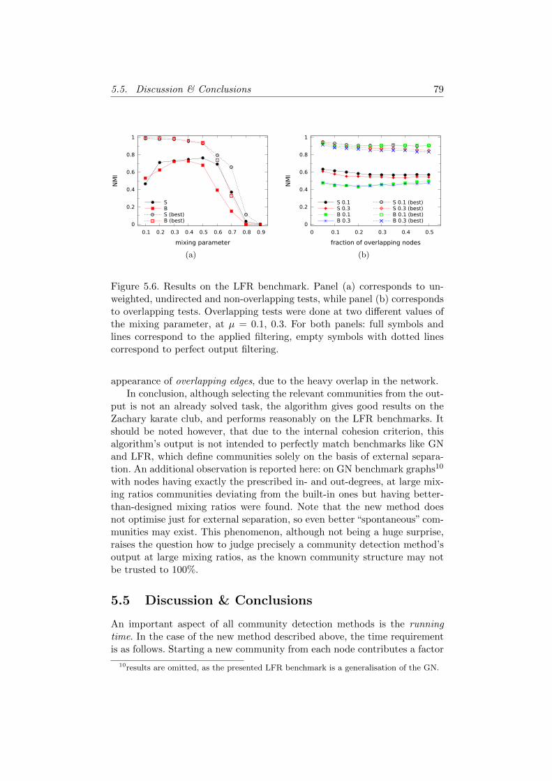
5.5. Discussion & Conclusions 79
0
0.2
0.4
0.6
0.8
1
0.1 0.2 0.3 0.4 0.5 0.6 0.7 0.8 0.9
NM
I
mixing parameter
SBS (best)B (best)
(a)
0
0.2
0.4
0.6
0.8
1
0 0.1 0.2 0.3 0.4 0.5
NM
I
fraction of overlapping nodes
S 0.1S 0.3B 0.1B 0.3
S 0.1 (best)S 0.3 (best)B 0.1 (best)B 0.3 (best)
(b)
Figure 5.6. Results on the LFR benchmark. Panel (a) corresponds to un-weighted, undirected and non-overlapping tests, while panel (b) correspondsto overlapping tests. Overlapping tests were done at two different values ofthe mixing parameter, at µ = 0.1, 0.3. For both panels: full symbols andlines correspond to the applied filtering, empty symbols with dotted linescorrespond to perfect output filtering.
appearance of overlapping edges, due to the heavy overlap in the network.In conclusion, although selecting the relevant communities from the out-
put is not an already solved task, the algorithm gives good results on theZachary karate club, and performs reasonably on the LFR benchmarks. Itshould be noted however, that due to the internal cohesion criterion, thisalgorithm’s output is not intended to perfectly match benchmarks like GNand LFR, which define communities solely on the basis of external separa-tion. An additional observation is reported here: on GN benchmark graphs10
with nodes having exactly the prescribed in- and out-degrees, at large mix-ing ratios communities deviating from the built-in ones but having better-than-designed mixing ratios were found. Note that the new method doesnot optimise just for external separation, so even better “spontaneous” com-munities may exist. This phenomenon, although not being a huge surprise,raises the question how to judge precisely a community detection method’soutput at large mixing ratios, as the known community structure may notbe trusted to 100%.
5.5 Discussion & Conclusions
An important aspect of all community detection methods is the runningtime. In the case of the new method described above, the time requirementis as follows. Starting a new community from each node contributes a factor
10results are omitted, as the presented LFR benchmark is a generalisation of the GN.
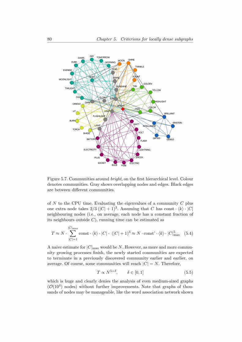
80 Chapter 5. Criterions for locally dense subgraphs
LAMP
BATTERY
GLOW
LIGHT
SHADE
DARK
FLASHLIGHT
EINSTEIN
VOLT
INTELLIGENTWATT
GIFTEDFLASH
GENIUS
BRILLIANT
NIGHT STARS
TWINKLESTAR
SQUINT
GOLDENTANSUNSHINE
FADE
SUN
YELLOW
HIGHLIGHT
BRIGHTCOLOR
MOONLIGHT
TWILIGHT
LIT
DIM
BURN
CANDLE
EVENING
TORCH
FUSEELECTRIC
SHOCK
LIGHTNING
PLUG
SOCKETBULB
ELECTRICITY
DAWN
DUSK
DAY TOMORROW
MORNINGMOON SHINE
Figure 5.7. Communities around bright, on the first hierarchical level. Colourdenotes communities. Gray shows overlapping nodes and edges. Black edgesare between different communities.
of N to the CPU time. Evaluating the eigenvalues of a community C plusone extra node takes 2/3 (|C| + 1)3. Assuming that C has const · 〈k〉 · |C|neighbouring nodes (i.e., on average, each node has a constant fraction ofits neighbours outside C), running time can be estimated as
T ≈ N ·|C|max∑|C|=1
const · 〈k〉 · |C| · (|C|+ 1)3 ≈ N · const’ · 〈k〉 · |C|5max (5.4)
A naive estimate for |C|max would be N . However, as more and more commu-nity growing processes finish, the newly started communities are expectedto terminate in a previously discovered community earlier and earlier, onaverage. Of course, some communities will reach |C| = N . Therefore,
T ∝ N5+δ, δ ∈ [0, 1] (5.5)
which is huge and clearly denies the analysis of even medium-sized graphs(O(104) nodes) without further improvements. Note that graphs of thou-sands of nodes may be manageable, like the word association network shown
5.5. Discussion & Conclusions 81
above, which took 56 hours on a single CPU. One possibility is to choose theinitial seed more intelligently, starting communities from promising seeds.[139] achieved good results in this aspect. An intelligent seed selection isalso important if the number of communities in a cover is larger than N ,or if some communities have only overlapping nodes – in this case, it mayhappen that all growth processes miss a certain community.Other important question is the applicability of an advanced eigenvaluesolver. Arpack++ [178] and SLEPc [179] were tried. The experience wasthat – despite their good asymptotic performance in the large matrix limit –for the occurring several small subgraphs the overhead of these complicatedmachineries was so large that made the final running time much higher thanthose obtained with the QR-decomposition algorithm.Doing optimisation in a multi-parameter space is a nontrivial task, becausedifferent parameters can lie in different ranges. Therefore, an important di-rection for future research is to investigate the best combination of the pa-rameters in the fitness function, based on the evaluation of empirical data.Finally, filtering the relevant communities from the found ones is also achallenging task. The natural approach is to apply statistical significance,which should be applied even if filtering was not needed. However, decidingthe threshold significance value is not necessarily trivial in all cases. Fur-thermore, the current form of statistical significance accounts only for theseparation of the community, not for its internal cohesion. This manifestsitself e.g. in the low score of the almost-full-clique subgraph in the Zacharykarate club (the dark purple group on Fig. 5.4). As the main advantageof the fitness function of eq. 5.3 is the inclusion of cohesion, it would beimportant to develop a statistical significance taking it into account.
Conclusions. The community detection problem currently suffers fromtwo fundamental deficiencies. First, there is no definition of communitywhich is precise enough to allow constructing community finding methods.Second, thorough testing a proposed algorithm is problematic, not indepen-dently from the previous difficulty. I attempted to improve both issues.
I proposed a formal list of required properties for locally dense subgraphs,taking a step towards an applicable definition of the term“community”. Twoproperties, external separation and internal cohesion (“shape”) were named.External separation has already been applied by some of the communitydetection methods, and also by benchmarks. Internal cohesion was not con-sidered explicitly earlier. No current method was found which satisfactorilyapplies both criterions. I demonstrated on simple examples that both proper-ties are necessary; discarding either of them leads to counterintuitive results.Beyond allowing to construct new methods, these two criterions can also beused as a basis for testing existing ones. They also allow the characterisationof a community by two independent quantities, instead of a single scalar.
I proposed a new composite fitness function which takes the two cri-terions into account. For the quantification of the internal cohesion of a

82 Chapter 5. Criterions for locally dense subgraphs
subgraph, the second eigenvalue of the Laplacian matrix (of the subgraph)is applied, which provides appropriate results on characteristic graphs likecliques or chains. I also proposed a heuristic, by redesigning the LFK heuris-tic [116], which can find strongly overlapping locally dense subgraphs of allscales, producing much less output than multiresolution methods but with-out the restrictions implied by assuming a hierarchical structure. Runs onthe Zachary network and LFR benchmarks showed that the method is ableto provide the expected results. Overlapping communities can be detectedespecially efficiently, similarly to other LFK-based heuristics [139]. However,significant improvements are yet to be implemented; e.g. reducing the run-ning time, finding a more effective filtering procedure for the output, orfine-tuning the relative weight of the separation and the cohesion terms inthe fitness function.

Chapter 6
Telecommunication networkplanning
6.1 Introduction
This work was done as a joint project of Nokia Siemens Networks and theBudapest University of Technology and Economics.
6.1.1 Problem definition
This chapter considers designing telecommunication networks. The telecom-munication network (abbreviated as network from this point) design canbe formulated as follows: given a set of nodes, a set of edges between thenodes (representing possible physical connections), a set of traffic demandsbetween the nodes, and a set of available equipments with their prices, finda set of equipments with their proper connections which satisfies the trafficdemands at the lowest possible cost.1
The aim of this chapter is to improve the existing solutions in this aspect,by introducing a new cluster-based design.
6.1.2 Motivation
Efficiently designing a telecommunication network which satisfies a given setof traffic demands is a hard task, exact optimal solutions can be reached onlyfor very small-sized networks. For larger networks, usually a set of heuristicsare applied to achieve as good results as possible.A possible approach is to partition the network into clusters, and designclusters separately. Due to their small size, clusters can be designed effi-ciently. The traffic crossing the clusters may be routed via one node in each
1This also includes determining the so-called logical links of the electrical layer (seeSec. 6.1.3).
84 Chapter 6. Telecommunication network planning
cluster (the hub node of the cluster), and the set of the hubs can be designedas an extra cluster. This way, the problem of designing a large network (thehardness of finding a good solution) can be reduced to the design of severalindependent small networks, which is a much easier problem.
6.1.3 Short introduction to network planning
The task of network planning is to satisfy a given set of traffic demands(like “10Gb/s from Hannover to Dortmund”) between a given set of sites(e.g. cities), represented as network nodes in the design process. The pos-sible physical connections between sites are also fixed. In this work, theresulting network will consist of only two layers, an electric (OTN) andan optical (DWDM) one. Layers correspond to different technologies in thenetwork. The optical layer consists of the optical cables and the devicessending/receiving optical signals through the optical cables. The electricallayer consists of electronic devices sending and receiving electronic signals.The two layers are in a hierarchical relationship: the original traffic demandto be served steps into the network as an electrical signal, and handled bysome electronic devices first, which pass it “down” to the optical devices fortransmission. After roaming a bit in the optical cables, the signal comes“up” to the electronic layer (e.g. to an Ethernet card) at its destination. Theintermediate sites between the source and the destination can be passed inthe optical layer, without touching their electrical layer, meaning that noelectronic resources are needed by the passing traffic. The task is to planthe detailed flow of all the traffic to be served, considering all technologicallayers. From this detailed plan, the necessary devices can be read out, andtheir prices give the cost of the network, which should be minimised. Themain problem is to find an optimal route for each demand. At first sight, itis as easy as to find the shortest paths between the sources and their tar-gets, which is indeed a valid solution. However, this design wastes a lot ofresources, as most devices will serve a single traffic demand, which is usuallymuch smaller than the available capacity of the allocated devices. Therefore,a good routing should take into account all traffic demands simultaneouslyin order to require only a few fully utilised devices, shared by many de-mands. This should be true both for the electrical and for the optical layers.For the optical layer, it means that as few fibers should be used as possible(although for realisations using protected paths this is dominated by theeffect of grooming, see a few lines later). That can be achieved by choosingroutes for different traffic demands such that they share as many fibers aspossible. This is a hard geometrical problem in alone, but unfortunately itis coupled to the other hard problem of the electrical layer. In the electricallayer, which consists of Ethernet cards at the sites, the problem is to spendas few money on the cards as possible. It can be reached either by a highutilisation of the cards or using cards with the best capacity/price ratio,
6.1. Introduction 85
or preferably both. Cards have a number of ports of varying capacity. Theaim is to utilise high as many ports on each cards as possible, in order tospare the allocation of additional cards. To this end, traffic demands maybe re-routed and broken into pieces, such that each piece terminates in theelectrical layer. This procedure, called grooming, is a fundamental optimisa-tion method. For further reading, see e.g. [205]-[207].A further difficulty is that alternative routes are usually also required, as aprotection against failures. The alternative paths may exclude the links ofthe original path, the nodes, or both. For efficient planning, the protectedand unprotected cases require different optimisation methods.
6.1.4 Input data
The working environment in which the new designing methods described inthis document were tested consists of the followings.
7 realistic test cases were used: Cost266, G17, G50, NewYork, Nobel-US,Pioro40, TA2. All of them consist of one set of traffic demands and onenetwork of possible physical connections between sites in a certain countryof city. The networks of physical connections are displayed on Figs. 6.2-6.3on pages 94-95, and some basic characteristics are summarised in Table 6.1.For simplicity, the test cases will be denoted by the single word “network”.The physical networks’ sizes, measured in the number of nodes (sites), rangefrom 14 (Nobel-US) to 65 (TA2). On average, the nodes have 2-6 physicalconnections, so the physical networks are quite sparse. Physical connectionsare usually made between geographically close nodes. Contrasting the phys-ical links, the traffic demands form a dense network, the majority of nodepairs possessing a demand. The test networks are all freely accessible fromthe SNDlib library [208].
The telecommunication network to be designed is modelled by two layers:an optical layer and an electrical layer. The optical layer consists of fibersbetween sites, 2 PXC (Photonic Cross-Connect) equipments at each end ofa fiber, and DWDM shelves containing the PXCs (providing power supply,mechanical protection, etc.). Each DWDM shelf can support only a limitednumber of PXCs. The electrical layer consists of electronic cards of varyingnumber of ports, which, in turn, can be of various capacities. E.g. a card canhave 16 ports, each with a capacity of 1Gb/s, and another card can have2 ports of 40Gb/s. There are also basenodes for supporting the electroniccards (providing power supply, mechanical protection, etc.). The number ofavailable slots for cards on each basenode is limited.
Exhaustive optimisation by network designing tools can be done for net-works up to 20-30 nodes. For a more efficient planning, a natural idea isto partition the network into small groups such that the groups have muchlarger traffic demands inside than outside. Then, each cluster can be designedindependently, using only the inside demands, and the inter-cluster traffic

86 Chapter 6. Telecommunication network planning
name N Lphys 〈k〉phys Ldem ρdemCost266 37 44 2.4 666 1
G17 17 26 3.1 121 0.89G50 50 88 3.5 662 0.54
NewYork 16 49 6.1 120 1Nobel-US 14 21 3.0 91 1Pioro40 40 89 4.5 780 1
TA2 42(65) 108 3.3 807 0.93
Table 6.1. List of test networks. N is the number of node, Lphys is thenumber of physical links, 〈k〉phys is the mean physical link degree, Ldem isthe number of undirected traffic demands, and ρdem is the ratio of Ldem toN(N − 1)/2. TA2 has some nodes without any traffic demand; the networksize including them is presented in parentheses.
can be designed later as a small correction. Unfortunately, for backbone net-works like the ones in Table 6.1 the existence of such an almost disconnectedpartitioning is not expected. Table 6.1 shows that the considered networksare indeed dense, usually fully connected. Efficient designing needs clustersnot larger than 20-30 nodes; for fully connected networks this requires thatthe inside links (traffic demands) should be much stronger than the out-side ones. For example, take a fully connected graph of N = 100 nodes andsearch for clusters having inside/outside traffic ratio of at least 3, and notlarger than 20 nodes. Then, on average, the inside traffic demands shouldbe at least 30 times larger than the outside ones. This is unreasonable; andindeed, experimenting with different clustering methods showed that suchpartitionings cannot be found [210].
6.2 New network designs
6.2.1 Overview
In this section, the traditional (flat) network design currently applied byNSN will be compared to hierarchical (clustered) and star topologies, tar-geting cost efficiency.
The hierarchical topology partitions the network into clusters and as-signs a hub node to each cluster. Any inter-cluster traffic demand is routedvia the corresponding hub nodes of the source and the target of the trafficdemand. For the intra-cluster traffic, there are two possible routing: usingthe shortest path between the source and the target, or routing via thehub2. Both strategies will be investigated. A schematic illustration of the
2A technical note for expert readers: in some cases, the post-processing optimisation
6.2. New network designs 87
hierarchical topology can be found on Fig. 6.1 a). Hierarchical topologieswere constructed using the clustering tool3 described on pages 87-89. Theapplied maximal cluster sizes for the test networks are the same as in Table6.2 on page 89. A few tests were done on the dependence of the results onthe maximal cluster sizes, but the results did not change very strongly overdifferent reasonable max. cluster sizes.
In the star topology, there are no clusters. One hub node is assigned tothe whole network, and all traffic demands are routed via the global hub.This is also true for traffic demands originating far from the hub in termsof optical links; in their case the the traffic travels along some intermedi-ate nodes before reaching the hub. Star topologies are also built using theclustering tool of Sec. 6.2.2, because it is a special case of the hierarchi-cal topology, using only one cluster and via-hub intra-cluster routing. Aschematic illustration of the star topology can be found on Fig. 6.1 b).
All network designs were built by the current4 MLO software (Multi-Layer Optimization, a custom network planning tool developed and appliedby NSN), using a realistic cost model. The relative equipment prices (com-pared to each other) are confidential, therefore they are not shown. Costs ofthe networks are given in a fictive unit, not in real currency. The differenttopologies were tested on the networks described in Sec. 6.1.4.
It should be noted here that all network designs are protectionless, i.e.for each traffic demand only 1 route is constructed. When implementing ina real network planning process, this issue should be addressed.
6.2.2 Clustering tool
During the NSN project a clustering tool was developed which integratesinto NSN’s network planning workflow, by reformatting the MLO networkplanning tool’s standard input such that running MLO on the new inputresults in a clustered network design.
The clustering tool applies the average-linkage hierarchical clustering topartition the network of physical connections into clusters. Although hier-archical clustering is much less sophisticated than the recent communitydetection methods, experiments showed that the telecommunication back-bone network problems have such a homogeneous structure that even thebest current methods were not able to produce really good partitions. Onthe other hand, hierarchical clustering has some practical advantages. Nev-ertheless, in section 6.2.3 Infomap will also be applied for comparison for
can alter the routing such that some routes are redirected and do not reach hubs. Thiscan affect both intra-cluster and inter-cluster routing.
3For G17, the result of the clustering tool was slightly modified by hand; node“Norden”was detached its original cluster and put in its own one. This was motivated by its demandstructure, consisting of a single demand to node 1.
4as of the autumn of 2010
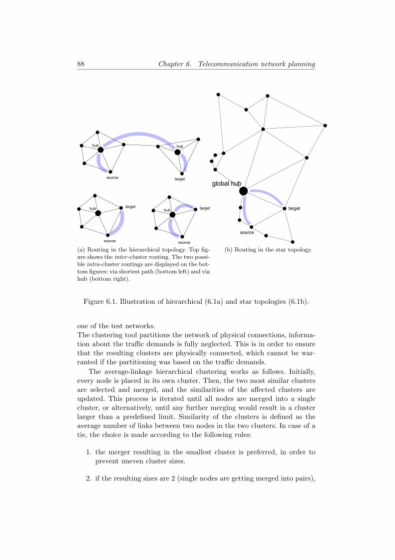
88 Chapter 6. Telecommunication network planning
source target
source
target
hub hub
hub
source
targethub
(a) Routing in the hierarchical topology. Top fig-ure shows the inter -cluster routing. The two possi-ble intra-cluster routings are displayed on the bot-tom figures: via shortest path (bottom left) and viahub (bottom right).
global hub
source
target
(b) Routing in the star topology.
Figure 6.1. Illustration of hierarchical (6.1a) and star topologies (6.1b).
one of the test networks.The clustering tool partitions the network of physical connections, informa-tion about the traffic demands is fully neglected. This is in order to ensurethat the resulting clusters are physically connected, which cannot be war-ranted if the partitioning was based on the traffic demands.
The average-linkage hierarchical clustering works as follows. Initially,every node is placed in its own cluster. Then, the two most similar clustersare selected and merged, and the similarities of the affected clusters areupdated. This process is iterated until all nodes are merged into a singlecluster, or alternatively, until any further merging would result in a clusterlarger than a predefined limit. Similarity of the clusters is defined as theaverage number of links between two nodes in the two clusters. In case of atie, the choice is made according to the following rules:
1. the merger resulting in the smallest cluster is preferred, in order toprevent uneven cluster sizes.
2. if the resulting sizes are 2 (single nodes are getting merged into pairs),

6.2. New network designs 89
the pair for which the sum of the two nodes’ degrees5 is minimal willbe merged. This is because low-degree nodes are supposed to haveneighbours from their own cluster, while a high-degree node may haveneighbours from many clusters.
This average-linkage hierarchical clustering has the following advantages:
• the clusters are always connected (since the clustering process finishesin the absence of nonzero similarities),
• it is very easy to prescribe an upper size limit for the clusters. Thus, itcan be ensured that the clusters remain small enough to be designedvery precisely,
• it is fast6.
Each cluster is assigned a hub node. For each cluster, the hub is selectedas
1. the node for which the sum of shortest paths to the other nodes in thecluster is minimal,
2. in case of a tie, the node for which the sum of shortest paths to allother nodes in the network is minimal.
The following maximal cluster sizes were applied:
Cost266 G17 G50 NewYork Nobel-US Pioro40 TA210 10 20 12 7 7 30
Table 6.2. Applied maximal cluster sizes for the test networks in the clus-tering tool.
6.2.3 Results
Using the “MLO” network planning tool of NSN, two hierarchical topologiesand a star topology were contrasted to the standard clusterless topology.The difference between the two hierarchical topologies is how they route theintra-cluster traffic: one topology uses shortest paths, the other routes allintra-cluster traffic via the hub of the cluster. Besides choosing a topology,there is also a tuning option in the MLO tool: it can be used in severalmodes, from which “basic” and “cost-based” were used.
5The degree of a node is the number of its neighbours.6The industrial partner required that the clustering process should not take more than
1-2 minutes, while the input might be even a dense network of several hundred nodes.

90 Chapter 6. Telecommunication network planning
fig:graphs1 The MLO tool was applied to the networks listed in Table 6.1:Cost266 (37 nodes), G17 (17 nodes), G50 (50 nodes), NewYork (16 nodes),Nobel-US (14 nodes), Pioro40 (40 nodes), TA2 (65 nodes).
The results are shown on Table 6.3. An immediate observation is thatconsidering the difference between the two clustered topologies, the one us-ing via-hub routing inside the clusters is always better than the other. Insome cases (NewYork, Nobel-US, G50) it happens that the “via-hub” topol-ogy is better than the traditional one, while the other is worse. For thesereasons, we will concentrate on the“via-hub”topology from the two clusteredalternatives.
Regarding the difference between the clustered and the traditional flattopology, results are mixed: for a number of networks (G17, TA2, G50,Nobel-US), the cluster-based topology is more efficient than the traditionalclusterless one. The gains are 18.3% (G17)7, 18.1% (TA2), 9.5% (G50), and4.8% (Nobel-US). On the other side, for some networks the traditional topol-ogy is the better (Cost266: −4.4%, NewYork: −2.3%, Pioro40: −2.1%).
On the G50 network, a different partitioning was also tested, obtainedby the Infomap partitioning method (see page 27). Its results are quite closeto those obtained by the default clustering, and tend to be somewhat worse.
A closer look on Table 6.3 shows that the potential advantage of theclustered topology lies in the usage of optical instruments (DWDM layer &fibers): in all cases when the “clusters-viahub” topology was better than thetraditional, the DWDM cost of the ”clusters-viahub“ network was lower thanthe traditional one. Not surprisingly, the fiber costs behave very similarly8.It suggests that the clustered networks can satisfy the traffic demands usingfewer physical links than the clusterless ones. On the other hand, the costsof the electronic cards (OTN layer) tend to be higher, due to the obliga-tory electronic termination of connections at the hubs (which effect can bereduced by MLO’s optimisation process). The success of the cluster-baseddesign depends on whether the gain in the optical (DWDM+fiber) layer ishigh enough to compensate the loss in the electrical (OTN) layer.
Although it is not straightforward to forecast whether the clusteredtopology is going to be better than the traditional one, there are some impor-tant notes. First of all, the cluster-based topology can only spare connectionsif there is a redundancy of physical links, i.e. on networks being close to atree the clustered topology has no potential advantage. The simplest man-ifestation of redundant connections is a triangle: 1/3 of its links may bespared. If one node in the triangle is a hub, then using only 2 links evennot increases the length of the shortest paths. There are two networks whichhave extremely low number of triangles, Cost266 (0 triangle) and Nobel-US (1 triangle). For Cost266, the traditional topology was indeed better.
7Percentages represent the best flat design and the best via-hub clustered design.8Fiber & DWDM costs both depends on the used fibers.

6.2. New network designs 91
Cost266 Hhub (b) Hsp (b) F (b) S (b) Hhub (c) Hsp (c) F (c) S (c)OTN 26757 26787 26712 26827 21167 21032 19447 21497DWDM 3372 3778 3438 3590 4444 4714 4986 4482Fibers 401 480 454 424 554 593 640 532total 30530 31045 30604 30841 26165 26339 25072.9 26511
G17OTN 1886 1856 1816 1916 906 906 906 921DWDM 756 1016 1104 696 756 1016 1104 696Fibers 86 108 130 72 86 108 130 72total 2728 2980 3050 2684 1748 2030 2140 1689
G50OTN 7251 7016 7271 7236 3611 3441 3271 3446DWDM 2470 3662 3932 2148 2998 4102 4020 2912Fibers 56 82 88 49 68 92 90 66total 9777 10760 11291 9433 6677 7635 7381 6424
G50-IMOTN 7216 7221 3636 3486DWDM 2468 3508 3100 4088Fibers 56 79 70 92total 9740 10808 6806 7666
NewYorkOTN 9022 8667 8677 9057 6247 5952 5032 5637DWDM 838 1832 2184 752 1406 2052 2404 1542Fibers 38 82 98 34 64 92 108 70total 9898 10581 10959 9843 7717 8096 7544 7249
Nobel-USOTN 4057 4032 4072 4087 4102 3987 3512 3897DWDM 660 944 944 574 660 944 944 574Fibers 3771 4461 4461 2633 3771 4461 4461 2633total 8488 9437 9477 7294 8533 9392 8917 7104
Pioro40OTN 112197 111932 111592 112212 112717 111702 110307 113572DWDM 12840 13632 11960 13280 6720 7780 7120 6636Fibers 57217 59319 47790 71264 29650 33122 28596 35787total 182254 184884 171342 196756 149087 152604 146023 155995
TA2OTN 10819 10739 10739 10714 8054 7749 7709 8199DWDM 2682 3578 3670 1994 4730 5310 4522 3734Fibers 9873 13367 14118 6547 17136 19434 16566 12356total 23374 27684 28527 19255 29920 32493 28797 24289
Table 6.3. Costs of the test networks. Lines correspond to types of cost (OTNis the electronic equipment, DWDM is the optical). Columns correspondto topology types: H is hierarchical, F is flat, S is star. The “hub” and“sp” subscripts refer to the intra-cluster routing method. In parentheses, theMLO optimisation mode is signed: (b) for basic, (c) for cost-based. The G50-IM subtable corresponds to results on the G50 network using the Infomapmethod for clustering.

92 Chapter 6. Telecommunication network planning
For Nobel-US, the clustered topology wins only due to the large fiber costs.Without fiber costs, the flat topology is the better one by 5.9%.This leads us to the second important factor, the price of the fibers andthe DWDM equipment. As the clustered topology can save on these costs,they should be high enough, compared to the OTN cost, in order to gainadvantage for the clustered topology.The question how much can be spared on the physical links is very important.However, it seems that it does not determine fully the success of the clus-tered topology. E.g. on the NewYork network, although the DWDM+fibercosts still take up 1/3 of the total cost and there is a very large abundanceof triangles, the flat topology is the better. For the Pioro40, it has less tri-angles and smaller DWDM+fiber cost / OTN cost ratio, but the clusteredtopology performs better than for the NewYork. It can be observed thatthese networks have a low average shortest path length (Table 6.4). Lowaverage shortest path length indicates that all regions of the network arewell connected to the rest of the graph, and this feature might make thetraditional topology more effective. Although it is a quite speculative argu-ment, it is interesting to note some features in Table 6.4. For NewYork, theaverage shortest path length is much shorter than for the similarly sized G17& Nobel-US. In case of NewYork, the flat topology is the better, in case ofG17 and Nobel-US, the clustered topology. For Pioro40, the average shortestpath is shorter than for the somewhat smaller Cost266 and the TA2.
name Nnodes N∆DWDM+fiber cost
OTN cost 〈l〉 cost(clustered)cost(flat)
Nobel-US 14 1 1.54 2.14 0.95NewYork 16 57 0.50 1.72 1.02G17 17 5 1.36 2.70 0.82Cost266 37 0 0.29 3.74 1.04Pioro40 40 39 0.32 3.31 1.02TA2 45 23 1.66 3.59 0.82G50 50 15 1.26 4.05 0.90
Table 6.4. Important features of the investigated networks: number of nodes,number of triangles, ratio of DWDM+fiber costs and OTN costs (for the bestflat design), mean shortest path length, ratio of best cluster-based cost andbest clusterless cost. Note: the TA2 network contains an additional 20 nodeswhich have no traffic demand and do not carry any shortest paths; thesenodes are not counted as they do not expected to alter the costs.
Considering the star topology, the same general observations holds asfor the clustered topology: it spares cost on the optical layer by using lessphysical links, and it is better than the traditional topology usually whenthe clustered topology is also better.
6.3. Conclusions 93
Apart from the results described above, an important observation is thatcost reduction can be achieved in connection with the choice of the shortestpaths. Shortest paths are often degenerate (more than one solution exist),and choices that maximise overlaps between shortest paths of different pairsof nodes can spare a number of physical links, with their corresponding PXCequipments.
6.3 Conclusions
To improve network planning efficiency a possible idea is to partition thenetwork into clusters. My investigation shows that using clusters can indeeddecrease the network cost, under certain conditions.
A first guess can be trying to separate the network into clusters suchthat the traffic between clusters is much smaller than inside clusters. Fornetworks having a dense traffic demand matrix (there is a traffic demandbetween most pairs of nodes) it is improbable that such a partitioning exists.
However, using clusters along with a well-chosen routing method canachieve more efficient network designs than the currently used clusterlessones, at least when each traffic demand is served by a single path (protec-tionless design). Including protection is expected to reduce the advantagesof the new designs. I created a clustering tool which partitions the networkand assigns a hub node to each cluster. The output of the tool is acceptedby NSN’s MLO network planning tool. Using this clustering tool with theMLO on test cases, I found that after partitioning the network, assigning ahub node to each cluster, and routing all traffic demands via the hubs of thesource and the target node’s hub, the total cost of the network was reducedby 5-18%, under proper conditions. In the unfavourable cases, cost increasedby 2-4%. Assigning a single hub node to the whole network gave comparableresults.
The new designs rely on reducing the number of used physical connec-tions. Consequently, for favourable performance, they require the presenceof redundant links in the input network, e.g. in the form of triangles, andalso require that the price of the equipments associated with the physicalconnections (optical devices) should be significant compared to the price ofother equipment (electronic cards). Low optical device prices or few redun-dant links mean that there is little to win by using the new designs, so thelosses in the electronic card costs may not be compensated. Less clear fac-tors also influence the performance; results suggest that the compactness ofthe network (quantified by low average shortest path length) also can givean advantage to the traditional clusterless design. On networks either hav-ing very few triangles, low optical equipment costs or being compact, thetraditional topology was better.
Along with these result, it was also found that when there are multiple
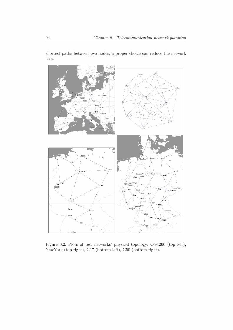
94 Chapter 6. Telecommunication network planning
shortest paths between two nodes, a proper choice can reduce the networkcost.
Figure 6.2. Plots of test networks’ physical topology: Cost266 (top left),NewYork (top right), G17 (bottom left), G50 (bottom right).
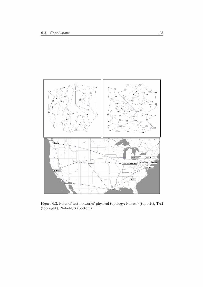
6.3. Conclusions 95
Figure 6.3. Plots of test networks’ physical topology: Pioro40 (top left), TA2(top right), Nobel-US (bottom).
Chapter 7
Summary
Clustering of objects is an old problem, however a general solution has notbeen found yet. A recently appeared interest from researchers working oncomplex networks resulted in significant improvements, although a majorpart of the work is still ahead. Even the most basic question, the definition ofclusters, called communities, is lacking, in spite of the apparent intuitivenessof the issue. The goal of this work is to contribute to the understanding andapplication of community structure in networks.
7.1 New scientific results
1. I showed that the label propagation method is equivalent to findingthe local minima of energy of a simple zero-temperature kinetic Pottsmodel. I found that 1) on the tested empirical networks, the number oflocal minima is unexpectedly large, 2) the algorithm is highly unstable,different runs resulting in different local minima [92].
2. For the matrix of the absolute values of correlation coefficients of stockreturns, which is equivalent to a weighted fully connected graph, Ifound that contrary to previous suggestions in the literature, the highranking eigenvectors are inappropriate for the identification of clusters,at least without further a priori information, because the eigenvectorsare frequently localised on combinations of clusters instead of singleclusters. Using diffusion-related matrices instead of the correlation ma-trix does not enhance the situation.I also found that the deviations of the first eigenvector’s componentsfrom the first-order perturbation theory are strongly correlated withthe square of the node strengths. Comparing it to a proper 0-model –an ensemble of matrices lacking cluster structure but otherwise havingsimilar features – I found that this feature is absent in the 0-model,consequently it can be attributed to the presence of cluster structure.
7.1. New scientific results 97
Checking the presence of clusters in correlation matrices can be donequicker in this way than by analysing the whole spectrum [136].
3. I defined a measure, tiling imperfection, for quantifying hierarchicalrelationship of partitions and covers. I found that on a multimillion-node, phone call data-based network, the results of different commu-nity detection methods – Infomap, Clique Percolation and modularityoptimisation by the Louvain method – have low tiling imperfections, inother words, they are quite close to each other, up to subset-supersetrelations [91].
4. I pointed out that the definition of communities should include notonly the property characterising the subgraph’s isolation from its sur-roundings, which I termed separation and was considered previously,but also cohesion – resistance against splitting into two –, thus I pro-posed a 2-dimensional system of requirements instead of the former1-dimensional criterion. I explicitly declared the required properties ofcommunities.I created a simple test for the two criterions. I proposed a measure forquantifying the cohesion of a subgraph, based on the second eigenvalueof the corresponding Laplacian matrix of the subgraph. I introduced anew community detection method, taking into account both separationand cohesion. The method is capable of handling strongly overlappingcommunities and multi-level structures. Tests were conducted on thestate-of-the-art benchmark (LFR), as well as on some real-world net-works [209].
5. For optimising telecommunication network planning, I elaborated amethod, which partitions the network into clusters, assigns a hub-nodeto each cluster and routes all traffic via the corresponding hubs. Underfavourable conditions, the costs of the test networks were reduced by5-18%, using the current network planning tool of Nokia Siemens Net-works. Redundant links, and not very compact networks are requiredfor success [210].

8. fejezet
Osszefoglalo
Regi problema kulonbozo objektumok csoportokba sorolasa (klaszterezese).Bar altalanos megoldas mindmaig nincs, az utobbi evekben a komplex halo-zatok teruleten dolgozo kutatok elenk erdeklodest mutattak a kerdes irant,komoly haladast eredmenyezve. Ennek ellenere a munka jelentos resze meghatravan. Meg a legalapvetobb kerdes, a
”suru csoport” definıcioja se tisz-
tazott, barmennyire intuitıvnak is tunjon. Jelen munka celja, hogy hozzaja-ruljon a halozatok csoportszerkezetenek megertesehez es felhasznalasahoz.
8.1. Uj tudomanyos eredmenyek
1. Megmutattam, hogy a label propagation csoportkereso modszer ekvi-valens egy egyszeru nulla homersekletu kinetikus Potts-modell lokalisenergia-minimumainak megkeresesevel. Valos halozatokat vizsgalva azttalaltam, hogy egyreszt a lokalis minimumok szama joval nagyobb avartnal, masreszt a modszer igen instabil, kulonbozo futtatasok kulon-bozo lokalis minimumokban vegzodnek [92].
2. Tozsdei hozamok korrelacios egyutthatoi abszolut ertekenek matrixatvizsgalva (ami ekvivalens egy sulyozott teljes graffal) megallapıtottam,hogy a matrix elso utan kovetkezo sajatvektorai - szemben a szakiro-dalomban talalhato javaslatokkal - alkalmatlanok a csoportok azono-sıtasara, legalabbis tovabbi elozetes informacio nelkul, mert a sajat-vektorok 1-1 csoport helyett sokszor csoportok kombinacioin lokalizal-tak. Diffuzio-alapu matrixokat alkalmazva korrelacios matrix helyett ahelyzet nem javul.A matrix elso sajatvektorarol megallapıtottam, hogy a komponensei-nek az elterese az elsorendu perturbacio-szamıtas eredmenyetol erosenkorrelalt a csomopontok erossegeinek negyzetevel. Ezt osszevetve egymegfelelo null-modellel - csoportszerkezet nelkuli, amde egyeb szem-pontokbol hasonlo matrixok sokasagaval - megallapıtottam, hogy a
8.1. Uj tudomanyos eredmenyek 99
korrelacio a null-modell eseten hianyzik, tehat jelenlete a csoportszer-kezet jelenletenek tulajdonıthato. Ez egy uj, a teljes spektrum elemze-senel gyorsabb eszkozt ad a csoportszerkezet jelenletenek ellenorzeserekorrelacios matrixokban [136].
3. Definialtam egy mennyiseget, a reszgrafok parkettazhatosaganak hi-bajat, ami partıciok es lefedesek hierarchikus viszonyait meri. Egytobb millio csomopontbol allo, telefonhıvas-adatokon alapulo haloza-ton kulonbozo csoportkereso modszerek - Infomap, klikk perkolacio esmodularitas-optimalizalas a Louvain modszerrel - eredmenyeit ossze-hasonlıtva megallapıtottam, hogy a kapott csoportok kis parkettazha-tosagi hibaval rendelkeznek, vagyis hasonloak, ha a reszhalmaz-anya-halmaz relacioktol eltekintunk [91].
4. Ramutattam, hogy a helyes csoport-definıcionak nemcsak az altalamszeparacionak nevezett, mar korabban vizsgalt, a csoporthoz tartozopontoknak a kornyezetuktol valo elkulonulesere jellemzo tulajdonsagotkell tartalmaznia, hanem a koheziot - ket reszre bontassal szembeniellenallast - is, vagyis a korabbi egydimenzios kriterium helyett egyketdimenzios kovetelmenyrendszert javasoltam. A csoportoktol elvarttulajdonsagokat explicit modon kimondtam.Keszıtettem egy egyszeru tesztet a kriteriumoknak valo megfeleles el-lenorzesere. Javaslatot tettem egy, a koheziot mero mennyiseg definıci-ojara, a reszgraf Laplace matrixanak masodik sajaterteke alapjan. Let-rehoztam egy uj csoportkereso eljarast, ami mind a szeparaciot, minda koheziot figyelembe veszi. A modszer kepes kezelni erosen atfedo estobbszintes csoportszerkezeteket is. A modszert teszteltem a jelenleglegjobbnak tekintett tesztgrafokon (LFR benchmark), es nehany valoshalozaton is [209].
5. Telekommunikacios halozatok optimalizacios tervezesere kidolgoztamegy modszert, amely a halozatot csoportokba osztja, minden csoport-hoz hozzarendel egy kozeppontot, es a teljes forgalmat a megfelelokozeppontokon keresztul iranyıtja. Megfelelo korulmenyek eseten a ha-lozat koltsegeit ıgy 5-18%-al lehetett csokkenteni a tesztek alapjan, aNokia Siemens Networks jelenlegi halozattervezo eszkozet hasznalva.A jo eredmenyhez redundans elek es nem tul kompakt halozat szukse-gesek [210].

Appendix A
Second eigenvalue of twoweakly connected cliques
Assume two cliques of n nodes, edge weights are 1. The two cliques areattached by a single edge having weight ε. Then the eigenvalue equationsfor the Laplacian matrix are∑
j<nj 6=i
xj + xn − (n− 1 + λ)xi = 0 ∀i < n (A.1)
∑k>nk 6=i
xk + xn+1 − (n− 1 + λ)xi = 0 ∀i > n+ 1 (A.2)
∑j<n
xj + ε · xn+1 − (n− 1 + ε+ λ)xi = 0 i = n (A.3)
∑k>n+1
xk + ε · xn − (n− 1 + ε+ λ)xi = 0 i = n+ 1 (A.4)
Adding the last two equations gives∑j
xj−xn−xn+1 +εxn+εxn+1− (n−1+ε+λ)xn− (n−1+ε+λ)xn+1 = 0
(A.5)The eigenvector corresponding to the first eigenvalue (which is zero) is theconstant vector, therefore for all other eigenvectors the sum of componentsshould be zero in order to be orthogonal to the first one. Consequently∑
j xj = 0. Applying this and a minimal algebra results
xn(λ+ n) + xn+1(λ+ n) = 0 (A.6)
xn = −xn−1 if λ 6= −n (A.7)
If λ = −n then eqs. A.1-A.2 reduce to∑
j≤n xj = 0 and∑
k≥n+1 xk = 0.Now consider the eigenspace corresponding to λ = −n, and look for eigen-vectors such that xn = xn+1 = c,
∑j<n xj = −c,
∑j>n+1 xj = −c. In this
101
eigenspace the number of free parameters are 1+2 ·(n−2), corresponding toc and x1 . . . xn−1, xn+2 . . . x2n with two constraints. Altogether the dimen-sion of the eigenspace (the multiplicity of λ = −n) is 2n − 3. Adding theλ = 0 case, we are left with at most two unknown eigenvalues.
For λ 6= −n, we look for the solutions in the form (a, . . . , a, b,−b,−a,N. . . ,−a)T .Then the eigenvalue equations are
(n− 2)a+ b− (n− 1 + λ)a = 0 (A.8)
(n− 1)a− ε · b− (n− 1 + ε+ λ)b = 0 (A.9)
After simplifications,
−(1 + λ)a+ b = 0 (A.10)
(n− 1)a− (n− 1 + 2ε+ λ)b = 0 (A.11)
Expressing λ from these equations reads
λ =b
a− 1 (A.12)
λ = −(n− 1 + 2ε) + (n− 1)a
b(A.13)
Writing λ = λ results
− n+ 1− 2ε+ (n− 1)a
b=b
a− 1 (A.14)
(−n+ 1− 2ε)b
a+ (n− 1) =
(b
a
)2
− b
a(A.15)
Introducing x = b/a gives
− x2 + (−n+ 2− 2ε)x+ (n− 1) = 0 (A.16)
x1,2 =n− 2 + 2ε±
√(n− 2 + 2ε)2 + 4(n− 1)
−2(A.17)
The term under the radical symbol can be approximated using the first twoterms of the Taylor series
√1− x ≈ 1− x/2
√. . . =
√(n+ 2ε)2
(1− 8ε
(n+ 2ε)2
)≈ (A.18)
≈ (n+ 2ε)
(1− 4ε
(n+ 2ε)2
)(A.19)
which gives
x1 ≈ 1− 2ε
n+ 2ε(A.20)
x2 ≈ 1− (n+ 2ε) +2ε
n+ 2ε(A.21)
102 Appendix A. Second eigenvalue of two weakly connected cliques
which, using eq. A.12, leads to
λ1 ≈ −2ε
n+ 2ε(A.22)
λ2 ≈ −(n+ 2ε) +2ε
n+ 2ε(A.23)
meaning that the last two eigenvalues of the Laplacian are found.
Appendix B
Review of currentcommunity detectionmethods
Here, a one-by-one review of methods follows, from the point of view of theseparation & cohesion criterions.
B.1 Separation-targeted methods
Method of Lancichinetti et al. (LFK) [116] – although being a mul-tiresolution method, it is informative to take a look at it with the resolutionparameter (see eq. 3.19) fixed at α = 1. Then the fitness function of a com-munity, which is to be optimised, is simply the sum of in-degrees divided bythe sum of degrees of the community members. Thus, this method is a clearimplementation of the separation criterion. Consequently, it is not sensitiveto the internal distribution of edges (Fig. 5.1a and 5.1b get the same fitness).The cohesion criterion is absent, so one clique on Fig. 5.1a has lower fitnessthan the union of the two cliques.Label propagation [77] – label propagation does not qualify the commu-nities, just finds partitions obeying the majority rule. Consequently Fig. 5.1acan be judged as a proper single community, and Fig. 5.1b can be split bycollecting each second node to the same cluster.Infomap [98] – it is straightforward to calculate that for the configura-tion on Fig. 5.1a, Infomap will properly separate the two cliques unless thenumber of inter-community links is larger than 6.9 · 107. Although this res-olution limit looks practically unimportant, shows that Infomap has someconceptual problems. If 3 edges are placed instead of 1 between the 2 cliqueson Fig. 5.1a, Infomap will merge the two cliques if the number of inter-community edges in the rest of the network is larger than 149, which ismore than 5 orders of magnitude smaller than the previous threshold. Two
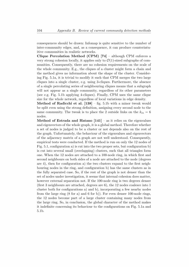
104 Appendix B. Review of current community detection methods
consequences should be drawn: Infomap is quite sensitive to the number ofinter-community edges, and, as a consequence, it can produce counterintu-itive communities in realistic networks.Clique Percolation Method (CPM) [74] – although CPM enforces avery strong cohesion locally, it applies only to O(1)-sized subgraphs of com-munities. Consequently, there are no cohesion requirements on the scale ofthe whole community. E.g., the cliques of a cluster might form a chain andthe method gives no information about the shape of the cluster. Consider-ing Fig. 5.1a, it is trivial to modify it such that CPM merges the two largecliques into a single cluster, e.g. using 3-cliques. Furthermore, the absenceof a single percolating series of neighbouring cliques means that a subgraphwill not appear as a single community, regardless of its other parameters(see e.g. Fig. 5.1b applying 4-cliques). Finally, CPM uses the same cliquesize for the whole network, regardless of local variations in edge density.Method of Radicchi et al. [138] – fig. 5.1b with a minor tweak wouldbe split even using the strong definition, assigning every second node to thesame community. The tweak is to place the 2 outside links on the kin = 6nodes.Method of Estrada and Hatano [141] – as it relies on the eigenvaluesand eigenvectors of the whole graph, it is a global method. Therefore whethera set of nodes is judged to be a cluster or not depends also on the rest ofthe graph. Unfortunately, the behaviour of the eigenvalues and eigenvectorsof the adjacency matrix of a graph are not well understood. Consequently,empirical tests were conducted. If the method is run on only the 12 nodes ofFig. 5.1, configuration a) is cut into the two proper sets, but configuration b)is cut into several small (overlapping) clusters, such that all triangles formone. When the 12 nodes are attached to a 100-node ring, in which first andsecond neighbours on both sides of a node are attached to the node (degreesare 4), then for configuration a) the two clusters expand to the first neigh-bouring nodes in the ring, and configuration b) has the same clusters as inthe fully separated case. So, if the rest of the graph is not denser than theset of nodes under investigation, it seems that internal cohesion does matter,however external separation not. If the 100-node ring is two degrees denser(first 3 neighbours are attached, degrees are 6), the 12 nodes coalesce into 1cluster both for configurations a) and b), incorporating a few nearby nodesfrom the large ring (8 for a) and 6 for b)). For even denser 100-node rings,the 12 nodes become part of a large cluster containing many nodes fromthe large ring. So, in conclusion, the global character of the method makesit indefinite concerning its behaviour to the configurations on Fig. 5.1a and5.1b.

B.2. Stochastic blockmodels and spin-based methods 105
B.2 Stochastic blockmodels and spin-based meth-ods
Modularity optimisation [73] – due to the well-known resolution limitproblem [78, 79], the optimal modularity merge the two cliques on Fig. 5.1afor sufficiently large graphs.Laplacian spectral algorithm by Donetti and Munoz [173] – althoughthe method produces candidate partitions using the spectrum of the Lapla-cian matrix, the partitions are evaluated using modularity. Consequently, itis equivalent to modularity optimisation using a special heuristic, implyingall the drawbacks of modularity.Link partitioning method of Evans and Lambiotte [117] – as the goalfunctions (variants of modularity) are based on counting intra-communityedges and subtracting some expected value, the resolution limit problemshould appear for large enough graphs.Method of Ronhovde and Nussinov (RN) [119] – the Hamiltonianoptimises simply for the edge densities inside clusters (distorted by the γ res-olution parameter), which tends to be the largest for cliques. ConsequentlyFig. 5.1b worth to be split into 4 if γ > 19/35. Similarly, for γ < 1/35, thetwo cliques of 5.1a are merged. The fact that the proper value of γ may varyfrom cluster to cluster can render the global optimisation process locallyunsuccessful.Method of Nepusz et al. [120] – the proposed method, when restrictedto conventional hard memberships (and unweighted networks), is equivalentto the previous method with γ = 1, and with a different heuristic.Stochastic blockmodel of Hofman and Wiggins [121] – a simple cal-culation for Fig. 5.1a shows that the two cliques will be merged if (1 −ϑc)/(1− ϑd) > 2−12/35(ϑd/ϑc)
1/35, which can be approximated by 1− ϑc >0.79(1 − ϑd), assuming that (ϑd/ϑc)
(1/35) ≈ 1. As ϑc corresponds to theintra-cluster edge probability, it is a reasonable criterion. Furthermore, it issimilarly simple to show that for Fig. 5.1b, splitting into four is profitable if(1− ϑd)/(1− ϑc) > 412/35(ϑc/ϑd)
19/35.Mixture model of Newman and Leicht [123] – considering Fig. 5.1band assuming hard node memberships (i.e. qir is 0 or 1 for all nodes), it iseasy to show that splitting into 4 is favoured over putting all nodes into onecluster.Mixture model of Wang and Lai [124] – for a hard clustering (qir = 0or 1) it is easy to calculate that Fig. 5.1b is preferred in 4 pieces over 1.Likelihood modularity of Bickel and Chen [127] – first, it should benoted that QLM penalises clusters in which the edge density deviates signif-icantly from its maximal value. Then, it is easy to calculate that it worth tocut Fig. 5.1b into 4 clusters.Stochastic blockmodel of Karrer and Newman [126] – it is similar to
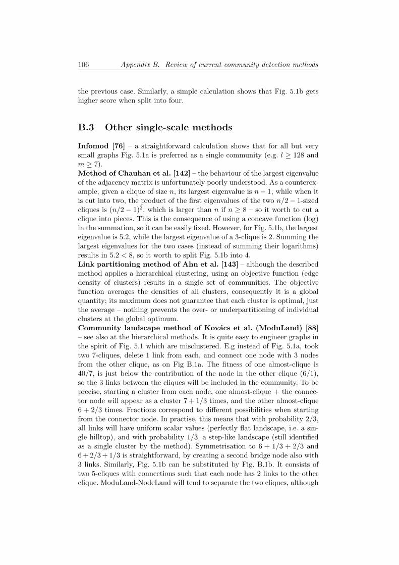
106 Appendix B. Review of current community detection methods
the previous case. Similarly, a simple calculation shows that Fig. 5.1b getshigher score when split into four.
B.3 Other single-scale methods
Infomod [76] – a straightforward calculation shows that for all but verysmall graphs Fig. 5.1a is preferred as a single community (e.g. l ≥ 128 andm ≥ 7).Method of Chauhan et al. [142] – the behaviour of the largest eigenvalueof the adjacency matrix is unfortunately poorly understood. As a counterex-ample, given a clique of size n, its largest eigenvalue is n− 1, while when itis cut into two, the product of the first eigenvalues of the two n/2− 1-sizedcliques is (n/2 − 1)2, which is larger than n if n ≥ 8 – so it worth to cut aclique into pieces. This is the consequence of using a concave function (log)in the summation, so it can be easily fixed. However, for Fig. 5.1b, the largesteigenvalue is 5.2, while the largest eigenvalue of a 3-clique is 2. Summing thelargest eigenvalues for the two cases (instead of summing their logarithms)results in 5.2 < 8, so it worth to split Fig. 5.1b into 4.Link partitioning method of Ahn et al. [143] – although the describedmethod applies a hierarchical clustering, using an objective function (edgedensity of clusters) results in a single set of communities. The objectivefunction averages the densities of all clusters, consequently it is a globalquantity; its maximum does not guarantee that each cluster is optimal, justthe average – nothing prevents the over- or underpartitioning of individualclusters at the global optimum.Community landscape method of Kovacs et al. (ModuLand) [88]– see also at the hierarchical methods. It is quite easy to engineer graphs inthe spirit of Fig. 5.1 which are misclustered. E.g instead of Fig. 5.1a, tooktwo 7-cliques, delete 1 link from each, and connect one node with 3 nodesfrom the other clique, as on Fig B.1a. The fitness of one almost-clique is40/7, is just below the contribution of the node in the other clique (6/1),so the 3 links between the cliques will be included in the community. To beprecise, starting a cluster from each node, one almost-clique + the connec-tor node will appear as a cluster 7 + 1/3 times, and the other almost-clique6 + 2/3 times. Fractions correspond to different possibilities when startingfrom the connector node. In practise, this means that with probability 2/3,all links will have uniform scalar values (perfectly flat landscape, i.e. a sin-gle hilltop), and with probability 1/3, a step-like landscape (still identifiedas a single cluster by the method). Symmetrisation to 6 + 1/3 + 2/3 and6 + 2/3 + 1/3 is straightforward, by creating a second bridge node also with3 links. Similarly, Fig. 5.1b can be substituted by Fig. B.1b. It consists oftwo 5-cliques with connections such that each node has 2 links to the otherclique. ModuLand-NodeLand will tend to separate the two cliques, although
B.4. Hierarchical methods 107
their union is much more well-separated from the rest of the graph.
(a) (b)
Figure B.1. Subgraphs on which ModuLand-NodeLand gives counterintu-itive results. Dashed lines show the desired communities.
B.4 Hierarchical methods
Here, some hierarchical methods will be investigated. The question is whetherthe lowest level can be reliably used as an optimal partition (or cover). Asa benchmark graph, Fig. B.2 will be utilised. The desired output is a singlecommunity of 12 nodes, due to their extreme separation from the rest of thegraph.Method of Ruan and Zhang [85] – the proposition is to iteratively
Figure B.2. Test case for the lowest level of the hierarchical methods.
run modularity optimisation in the found clusters, until the best modularityinside a cluster is not larger significantly than those of a corresponding ran-dom graph. Numerical calculations show that at the lowest level, Fig. B.2 isdivided into parts1.
1z-score is 5.3, Qmax = 0.36. Z-score is defined as the difference of the modularity of theactual graph and the modularity of a 0-model graph, divided by the standard deviation
108 Appendix B. Review of current community detection methods
Method of Sales-Pardo et al. [84] – it uses the co-occurrence of nodesin different local optima of modularity to construct a new similarity matrix,which is fitted by a block diagonal form. Communities are defined by theblocks. The method is iteratively re-applied to each community until struc-ture deviating from a corresponding random graph is found. Again, runningthe method on Fig. B.2 results in overpartitioning (z-score of the split Fig.B.2 is 3.9, the threshold used by [84] is 2.3).Hierarchical Infomap [86] – this is an extension of the Infomap method[98]. It is easy to calculate that, similarly to the previous cases, splitting Fig.B.2 on a lower hierarchical level improves the partition.ModuLand [88] – ModuLand can also produce hierarchical structures, byiteratively re-running the clustering procedure on the network of clusters(links between clusters are defined by node overlaps). Accordingly, the low-est level clusters are the ones obtained by a simple ModuLand run, which issusceptible to mispartitioning, as described some paragraphs above.OSLOM [94] – the method applies statistical significance as fitness. Al-though its output depends to a certain degree on the whole graph, runningit on Fig. B.2 (as the whole graph) results in a bisection. As the method triesto find the so-called minimal significant clusters, by trying to split alreadyfound significant subgraphs while the rest of the graph is neglected, it willdivide Fig. B.2 independently of the rest of the graph.
of the modularity of the 0-model graph, z-score = (Q − Q0-model)/σ0-model. Criterion of[85] is z-score ≥ 2, Qmax ≥ 0.3. Modularities were optimised using the Radatools software[211].
Bibliography
[1] A.-L. Barabasi: Linked: The New Science of Networks, Perseus BooksGroup (2002).Barabasi Albert-Laszlo: Behalozva: a halozatok uj tudomanya, MagyarKonyvklub (2003).
[2] M. Buchanan: Nexus: Small Worlds and the Groundbreaking Scienceof Networks, W. W. Norton & Company (2002).
[3] Csermely Peter: A rejtett halozatok ereje, Vince Kiado (2005).P. Csermely: Weak Links: Stabilizers of Complex Systems from Pro-teins to Social Networks, Springer (2006).
[4] S. Bornholdt, H. G. Schuster (eds.): Handbook of Graphs and Net-works: From the Genome to the Internet, Wiley-VCH (2003).
[5] D. J. Watts: Small Worlds: The Dynamics of Networks between Orderand Randomness, Princeton University Press (2003).
[6] R. Pastor-Satorras, A. Vespignani: Evolution and Structure of the In-ternet: A Statistical Physics Approach, Cambridge University Press(2004).
[7] E. Ben-Naim, H. Frauenfelde, Z. Toroczkai (eds.): Complex Networks,Springer (2004).
[8] National Research Council (U.S., ed.): Network Science, NationalAcademies Press (2005).
[9] M. Newman, A.-L. Barabasi, D. J. Watts: The Structure and Dynamicsof Networks, Princeton University Press (2006).
[10] S. N. Dorogovtsev, J. F. F. Mendes: Evolution of Networks: FromBiological Nets to the Internet and WWW, Oxford University Press,New York (2003).
[11] D. J. Watts, S. H. Strogatz, Collective dynamics of ’small-world’ net-works, Nature 393, 440-442 (1998).
110 Bibliography
[12] P. Erdos, A. Renyi, On random graphs, Publicationes MathematicaeDebrecen 6, 290-297 (1959).
[13] R. Albert, A.-L. Barabasi, Emergence of scaling in random networks,Science 286, 509-512 (1999).
[14] H. Jeong, B. Tombor, R. Albert, Z. Oltvai, A.-L. Barabasi, The large-scale organization of metabolic networks, Nature 407, 651-655 (2000).
[15] I. Farkas, H. Jeong, T. Vicsek, A.-L. Barabasi, Z. N. Oltvai, The topol-ogy of the transcription regulatory network in the yeast S. cerevisiae,Physica A 318, 601-612 (2003).
[16] T. Korcsmaros, I. J. Farkas, M. S. Szalay, P. Rovo, D. Fazekas, Z.Spiro, Cs. Bode, K. Lenti, T. Vellai, P. Csermely, Uniformly curatedsignaling pathways reveal tissue-specific cross-talks and support drugtarget discovery. Bioinformatics 26, 2042 (2010).
[17] Robert M. May, Stability and complexity in model ecosystems, Prince-ton University Press (2001).
[18] J. Loscalzo, I. Kohane, A.-L. Barabasi, Human disease classification inthe postgenomic era: A complex systems approach to human pathobi-ology, Molecular Systems Biology 3, 124 (2007).
[19] D. Lusseau, The emergent properties of a dolphin social network. Bi-ology Letters, Proc. R. Soc. London B (suppl.) (2003).
[20] J. Ø. H. Bakke, A. Hansen, J. Kertesz, Failure and avalanches in com-plex networks, Europhys. Lett. 76, 717 (2006).
[21] G. O’Danleyman, J. J. Lee, H. Seebens, B. Blasius, D. Brockmann,Complexity in human transportation networks: A comparative analy-sis of worldwide air transportation and global cargo ship movements,arXiv:1103.5451v1 (2011).
[22] C. M. Schneider, A. A. Moreira, J. S. Andrade Jr., S. Havlin, H. J.Herrmann, Mitigation of Malicious Attacks on Networks, PNAS 108,3838 (2011).
[23] S. Valverde, R. F. Cancho, R. V. Sole, Scale-free networks from optimaldesign, Europhys. Lett. 60, 512-517 (2002).
[24] R. F. Cancho, C. Janssen, R. V. Sole, Topology of technology graphs:Small world patterns in electronic circuits, Phys. Rev. E 64, 046119(2001).
Bibliography 111
[25] S. Carmi, S. Havlin, C. Song, K. Wang, H. A. Makse, Energy-landscapenetwork approach to the glass transition, J. Phys. A: Math. Theor. 42,105101 (2009).
[26] J. H. Snoeijer, T. J. H. Vlugt, M. van Hecke, W. van Saarloos, ForceNetwork Ensemble: A New Approach to Static Granular Matter, Phys.Rev. Lett. 92, 054302 (2004).
[27] S. C. Chae, Y. Horibe, D. Y. Jeong, S. Rodan, N. Lee, S.-W. Cheong,Self-organization, condensation, and annihilation of topological vor-tices and antivortices in a multiferroic, PNAS 107, 21366 (2010).
[28] S. H. Strogatz, Exploring complex networks, Nature 410, 268 (2001).
[29] R. Milo, S. Itzkovitz, N. Kashtan, R. Levitt, S. Shen-Orr, I. Ayzen-shtat, M. Sheffer, U. Alon, Superfamilies of Evolved and DesignedNetworks, Science 303, 1538-1542 (2004).
[30] Y.-M. Choi, H.-J. Kim, A Directed Network of Greek and RomanMythology, Physica A 382, 665 (2007).
[31] M. A. Serrano, M. Boguna, Topology of the world trade web, Phys.Rev. E 68, 015101 (2003).
[32] K. Yamasaki, A. Gozolchiani, S. Havlin, Climate Networks aroundthe Globe are Significantly Effected by El Nino, Phys. Rev. Lett. 100,228501 (2008).
[33] A. V. Goltsev, S. N. Dorogovtsev, J. F. F. Mendes, Percolation oncorrelated networks, Phys. Rev. E 78, 051105 (2008).
[34] A. V. Goltsev, S. N. Dorogovtsev, J. F. F. Mendes, Critical phenomenain complex networks, Rev. Mod. Phys. 80, 1275 (2008).
[35] J. D. Noh, H. Rieger, Random Walks on Complex Networks, Phys.Rev. E 92, 118701 (2004).
[36] R. Pastor-Satorras, A. Vespignani, Epidemic dynamics and endemicstates in complex networks, Phys. Rev. Lett. 86, 3200-3203 (2001).
[37] D. Garlaschelli, A. Capocci, G. Caldarelli, Self-organized network evo-lution coupled to extremal dynamics, Nature Physics 3, 813 (2007).
[38] Stefan Bornholdt, Less Is More in Modeling Large Genetic Networks,Science 310, 449 (2005).
[39] R. V. Donner, J. Heitzig, J. F. Donges, Y. Zou, N. Marwan, J. Kurths,The Geometry of Chaotic Dynamics – A Complex Network Perspec-tive, arXiv:1102.1853 (2011).
112 Bibliography
[40] M. Perc, A. Szolnoki, Coevolutionary games – a mini review, BioSys-tems 99, 109 (2010).
[41] K. D. Lafferty, J. A. Dunne, Stochastic ecological network occupancy(SENO) models, a new tool for analyzing ecological networks acrossspatial scales, Theoretical Ecology 3, 123 (2010).
[42] R. Albert, A.-L. Barabasi, Statistical Mechanics of Complex Networks,Rev. Mod. Phys. 74, 47 (2002).
[43] M. E. J. Newman, The structure and function of complex networks,SIAM Rev. 45, 167 (2003).
[44] S. Boccaletti, V. Latora, Y. Moreno, M. Chavez, D.-U. Hwang, Com-plex networks: Structure and dynamics, Phys. Reports 424, 175(2006).
[45] R. Cohen, S. Havlin, Scale-Free Networks are Ultrasmall, Phys. Rev.Lett. 90, 058701 (2003).
[46] R. Albert, H. Jeong, A.-L. Barabasi: Error and attack tolerance ofcomplex networks, Nature 406, 378 (2000).
[47] R. Pastor-Satorras, A. Vespignani, Epidemic spreading in scale-freenetworks, Phys. Rev. Lett. 86, 3200 (2001).
[48] V. Colizza, A. Flammini, M. A. Serrano, A. Vespignani, Detectingrich-club ordering in complex networks, Nature Physics 2, 110 (2006).
[49] S. Shen-Orr, R. Milo, S. Mangan, U. Alon, Network motifs in thetranscriptional regulation network of Escherichia coli, Nature Genetics,31, 64 (2002).
[50] M. L. Goldstein, S. A. Morris, G. G. Yen, Problems with fitting to thepower-law distribution, Eur. Phy. J. B 41, 255 (2004).
[51] R. Tanaka, T.-M. Yi, J. Doyle, Some protein interaction data do notexhibit power law statistics, FEBS Letters 579 514 (2005).
[52] C. Song, S. Havlin, H. A. Makse, Self-similarity of complex networks,Nature 433, 392 (2005).
[53] C. Song, S. Havlin, H. A. Makse Origins of fractality in the growth ofcomplex networks, Nature Physics 2, 275 (2006).
[54] K.-I. Goh, G. Salvi, B. Kahng, es D. Kim: Skeleton and fractal scalingin complex networks, Phys. Rev. Lett. 96, 018701 (2006).
Bibliography 113
[55] G. Palla, I. J. Farkas, P. Pollner, I. Derenyi, T. Vicsek, Fundamentalstatistical features and self-similar properties of tagged networks, NewJ. Phys. 10, 123026 (2008).
[56] R. Albert, H. G. Othmer, The topology of the regulatory interactionspredicts the expression pattern of the Drosophila segment polaritygenes, J. Theor. Biology 223, 1 (2003).
[57] A. E. Motter, N. Gulbahce, E. Almaas, A.-L. Barabasi, Predictingsynthetic rescues in metabolic networks, Molecular Systems Biology4, 168 (2008).
[58] S. Sahasrabudhe, A. E. Motter, Rescuing ecosystems from extinctioncascades through compensatory perturbations, Nature Communica-tions 2, 170 (2011).
[59] J.-P. Onnela, J. Saramaki, J. Hyvonen, G. Szabo, M. A. de Menezes, K.Kaski, A.-L. Barabasi, J. Kertesz, Analysis of a large-scale weightednetwork of one-to-one human communication, New J. Phys. 9 179(2007).
[60] L. Euler, Solutio Problematis ad Geometriam Situs Pertinentis, Com-mentarii Academiae Scientiarum Imperialis Petropolitanae 8 128(1741) = Opera Omnia (1), Vol. 7, 1-10.
[61] O. Boruvka, Acta Societ. Scient. Natur. Moraviae, 3 37 (1926).
[62] V. D. Blondel, J.-L. Guillaume, R. Lambiotte, E. Lefebvre, Fast un-folding of communities in large networks, J. Stat. Mech. P10008 (2008).
[63] C. A. Hidalgo, B. Klinger, A.-L. Barabasi, R. Hausmann, The productspace conditions the development of nations, Science 317 482 (2007).
[64] S. Wasserman, K. Faust: Social Network Analysis, Cambridge Univer-sity Press, (1994).
[65] S. Fortunato, Community detection in graphs, Phys. Rep. 486, 75(2010).
[66] M. Blatt, S. Wiseman, E. Domany, Super-paramagnetic clustering ofdata, Phys. Rev. Lett. 76, 3251 (1996).
[67] J.-P. Eckmann, E. Moses, Curvature of co-links uncovers hidden the-matic layers in the World Wide Web, PNAS 99, 5825 (2002).
[68] S. Maslov, K. Sneppen, Specificity and Stability in Topology of ProteinNetworks, Science 296, 910 (2002).

114 Bibliography
[69] M. Girvan, M. E. J. Newman, Community structure in social andbiological networks, PNAS 99, 7821 (2002).
[70] J. Podani, Z. N. Oltvai, H. Jeong, B. Tombor, A.-L. Barabasi, E.Szathmary, Comparable system-level organization of Archaea and Eu-karyotes, Nature Genetics 29, 54 (2001).
[71] E. Ravasz, A. L. Somera, D. A. Mongru, Z. N. Oltvai, A.-L. Barabasi,Hierarchical Organization of Modularity in Metabolic Networks, Sci-ence 297, 1551 (2002).
[72] F. Wu, B.A. Huberman, Finding communities in linear time: a physicsapproach, Eur. Phys. J. B 38, 331 (2004).
[73] M. E. J. Newman, M. Girvan, Finding and evaluating communitystructure in networks, Phys. Rev. E 69, 026113 (2004).
[74] G. Palla, I. Derenyi, I. Farkas, T. Vicsek, Uncovering the overlappingcommunity structure of complex networks in nature and society, Na-ture 435, 814 (2005).
[75] S. Sreenivasan, H. Kim, Z. Toroczkai, Emergence of functional modu-larity in multitasking networks, preprint (2010).
[76] M. Rosvall, C. T.Bergstrom, An information-theoretic framework forresolving community structure in complex networks, PNAS 104 7327(2007).
[77] U. N. Raghavan, R. Albert, S. Kumara, Near linear time algorithm todetect community structures in large-scale networks, Phys. Rev. E 76036106 (2007).
[78] S. Fortunato, M. Barthelemy, Resolution limit in community detection,PNAS 104 36 (2007).
[79] J. M. Kumpula, J. Saramaki, K. Kaski, J. Kertesz, Limited resolutionin complex network community detection with Potts model approach,Eur. Phys. J. B 56, 41 (2007).
[80] J. M. Kumpula, J. Saramaki, K. Kaski, J. Kertesz, Limited resolutionand multiresolution methods in complex network community detec-tion, Fluct. Noise Lett. 7, L209 (2007).
[81] J. Reichardt, S. Bornholdt, Statistical mechanics of community detec-tion, Phys. Rev. E 74, 016110 (2006).
[82] A. Arenas, A. Fernandez, S. Gomez, Analysis of the structure of com-plex networks at different resolution levels, New J. Phys. 10, 053039(2008).

Bibliography 115
[83] J.-C. Delvenne, S. N. Yaliraki, M. Barahona, Stability of graph com-munities across time scales, PNAS 107, 12755 (2010).
[84] M. Sales-Pardo, R. Guimera, A. A. Moreira, L. A. N. Amaral, Ex-tracting the hierarchical organization of complex systems, PNAS 104,15224 (2007).
[85] J. Ruan, W. Zhang, Identifying network communities with a high res-olution, Phys. Rev. E 77, 016104 (2008).
[86] M. Rosvall, C. T. Bergstrom, Multilevel compression of random walkson networks reveals hierarchical organization in large integrated sys-tems, arXiv:1010.0431v1 (2010).
[87] A. V. Esquivel, M. Rosvall, Compression of flow can reveal overlappingmodular organization in networks, arXiv:1105.0812v1 (2011).
[88] I. A. Kovacs, R. Palotai, M. S. Szalay, P. Csermely, Community Land-scapes: An Integrative Approach to Determine Overlapping NetworkModule Hierarchy, Identify Key Nodes and Predict Network Dynam-ics, PLoS ONE 5, 12528 (2010).
[89] R. Guimera, M. Sales-Pardo, L. A. N. Amaral, Modularity from fluc-tuations in random graphs and complex networks, Phys. Rev. E 70,025101 (2004).
[90] B. H. Good, Y.-A. de Montjoye, A. Clauset, Performance of modularitymaximization in practical contexts, Phys. Rev. E 81, 046106 (2010).
[91] G. Tibely, M. Karsai, L. Kovanen, K. Kaski, J. Kertesz, J. Saramaki,Communities and beyond: mesoscopic analysis of a large social networkwith complementary methods, Phys. Rev. E 83, 056125 (2011).
[92] G. Tibely, J. Kertesz, On the equivalence of the label propagationmethod of community detection and a Potts model approach, PhysicaA 387, 4982 (2008).
[93] A. Lancichinetti, F. Radicchi, J.J. Ramasco, Statistical significance ofcommunities in networks, Phys. Rev. E 81, 046110 (2010).
[94] A. Lancichinetti, F. Radicchi, J. J. Ramasco, S. Fortunato, Find-ing statistically significant communities in networks, arXiv:1012.2363(2010).
[95] U. Brandes, D. Delling, M. Gaertler, R. Goerke, M. Hoefer, Z.Nikoloski, D. Wagner, On Modularity Clustering, IEEE Trans. Knowl.Data Eng. 20, 172 (2008).
116 Bibliography
[96] A. Lancichinetti, S. Fortunato, Community detection algorithms: acomparative analysis, Phys. Rev. E 80, 056117 (2009).
[97] K. A. Eriksen, I. Simonsen, S. Maslov, K. Sneppen, Modularity andExtreme Edges of the Internet, Phys. Rev. Lett. 90, 148701 (2003).
[98] M. Rosvall, C. T. Bergstrom, Maps of information flow reveal commu-nity structure in complex networks, PNAS 105 1118 (2008).
[99] M. T. Schaub, R. Lambiotte, M. Barahona, Coding of Markov dy-namics for multiscale community detection in complex networks,arXiv:1109.6642 (2011).
[100] A. Clauset, Finding local community structure in networks, Phys. Rev.E 72, 026132 (2005).
[101] W. W. Zachary, An Information Flow Model for Conflict and Fissionin Small Groups, J. Anthropol. Res. 33, 452 (1977).
[102] A. Lancichinetti, S. Fortunato, F. Radicchi, Benchmark graphs fortesting community detection algorithms, Phys. Rev. E 78, 046110(2008).
[103] A. Lancichinetti, S. Fortunato, Benchmarks for testing community de-tection algorithms on directed and weighted graphs with overlappingcommunities, Phys. Rev. E 80, 016118 (2009).
[104] J. MacQueen, Some methods for classification and analysis of multi-variate observations, Proc. Fifth Berkeley Symp. on Math. Statist. andProb. 281–297 (1967).
[105] R. S. Tsay, Analysis of Financial Time Series, John Wiley (2002).
[106] R. Sokal, C. Michener, A statistical method for evaluating systematicrelationships, University of Kansas Science Bulletin 38, 1409 (1958).
[107] T. Hastie, R. Tibshirani, J. Friedman, The Elements of StatisticalLearning: Data Mining, Inference, and Prediction, Springer-Verlag(2009).
[108] P. Boldi, M. Rosa, M. Santini, S. Vigna, Layered Label Propagation:A MultiResolution Coordinate-Free Ordering for Compressing SocialNetworks, arXiv:1011.5425 (2010).
[109] A. Capocci, V. D. P. Servedio, G. Caldarelli, F. Colaiori, Detectingcommunities in large networks, Physica A 352, 669 (2005).
[110] M. Latapy, P. Pons, Computing Communities in Large Networks UsingRandom Walks, Lect. Notes Comp. Sci. 3733, 284 (2005).
Bibliography 117
[111] H. Zhou, Distance, dissimilarity index, and network community struc-ture, Phys. Rev. E 67, 061901 (2003).
[112] R. Lambiotte, J.-C. Delvenne, M. Barahona, Laplacian Dynamics andMultiscale Modular Structure in Networks,. arXiv:0812.1770 (2008).
[113] G. Krings, V. D. Blondel, An upper bound on community size in scal-able community detection, arXiv:1103.5569 (2011).
[114] A. Lancichinetti, S. Fortunato, Limits of modularity maximization incommunity detection, arXiv:1107.1155 (2011).
[115] V. A. Traag, P. Van Dooren, Y. Nesterov, Narrow scope for resolution-free community detection, arXiv:1104.3083 (2011).
[116] A. Lancichinetti, S. Fortunato, J. Kertesz, Detecting the overlappingand hierarchical community structure of complex networks, New J. ofPhys. 11 033015 (2009).
[117] T. Evans, R. Lambiotte, Line graphs, link partitions, and overlappingcommunities, Phys. Rev. E 80, 016105 (2009).
[118] T. S. Evans, Clique Graphs and Overlapping Communities, J. Stat.Mech. P12037 (2010).
[119] P. Ronhovde, Z. Nussinov, Multiresolution community detection formegascale networks by information-based replica correlations, Phys.Rev. E 80, 016109 (2009).
[120] T. Nepusz, A. Petroczi, L. Negyessy, F. Bazso, Fuzzy communitiesand the concept of bridgeness in complex networks, Phys. Rev. E 77016107 (2008).
[121] J. M Hofman, C. H. Wiggins, Bayesian Approach to Network Modu-larity, Phys. Rev. Lett. 100, 258701 (2008).
[122] M. B. Hastings, Community Detection as an Inference Problem, Phys.Rev. E 74 035102 (2006).
[123] M. E. J. Newman, E. A. Leicht, Mixture models and exploratory anal-ysis in networks, PNAS 104 9564 (2007).
[124] J. Wang, C-H Lai, Detecting groups of similar components in complexnetworks, New J. Phys. 10, 123023 (2008).
[125] A. McDaid, N.J. Hurley, Detecting highly overlapping communitieswith Model-based Overlapping Seed Expansion, ASONAM 2010
[126] B. Karrer, M. E. J. Newman, Stochastic blockmodels and communitystructure in networks, Phys. Rev. E 83, 016107 (2011).
118 Bibliography
[127] P. J. Bickel, A. Chen, A nonparametric view of network models andNewman–Girvan and other modularities, PNAS 106, 21068 (2009).
[128] S. Gregory, Finding overlapping communities in networks by labelpropagation, New J. Phys. 12, 103018 (2010).
[129] M. J. Barber, J. W. Clark, Detecting network communities by propa-gating labels under constraints, Phys. Rev. E 80, 026129 (2009).
[130] I. X. Y. Leung, P. Hui, P. Lio, J. Crowcroft, Towards real-time com-munity detection in large networks, Phys. Rev. E 79, 066107 ((2009).
[131] L. Subelj, M. Bajec, Unfolding communities in large complex networks:Combining defensive and offensive label propagation for core extrac-tion, Phys. Rev. E 83, 036103 (2011).
[132] L. Subelj, M. Bajec, Robust network community detection using bal-anced propagation, Eur. Phys. J. B 81, 353 (2011).
[133] C. M. Fortuin, P. W. Kasteleyn: On the random-cluster model, Physica57, 536-564 (1972).
[134] I. J. Farkas, D. Abel, G. Palla, T. Vicsek, Weighted network modules,New J. Phys. 9, 180 (2007).
[135] G. Palla, I. J. Farkas, P. Pollner, I. Derenyi, T. Vicsek, Directed net-work modules, New J. Phys. 9, 186 (2007).
[136] T. Heimo, G. Tibely, J. Saramaki, K. Kaski, J. Kertesz, Spectral meth-ods and cluster structure in correlation-based networks, Physica A387, 5930 (2008).
[137] A. Clauset, C. Moore, M. E. J. Newman, Hierarchical structure andthe prediction of missing links in networks, Nature 453, 98 (2008).
[138] F. Radicchi, C. Castellano, F. Cecconi, V. Loreto, D. Parisi, Definingand identifying communities in networks, PNAS 101 2658 (2004).
[139] C. Lee, F. Reid, A. McDaid, N. Hurley, Detecting highly overlappingcommunity structure by greedy clique expansion, arXiv:1002.1827v1(2010).
[140] F. Havemann, M. Heinz, A. Struck, J. Glaser, Identification ofoverlapping communities and their hierarchy by locally calculatingcommunity-changing resolution levels, J. Stat. Mech. P01023 (2011).
[141] E. Estrada, N. Hatano, Communicability in complex networks, Phys.Rev. E 77, 036111 (2008).
Bibliography 119
[142] S. Chauhan, M. Girvan, E. Ott, Using Network Function to Defineand Identify Community Structure, arXiv:0911.2735v1 (2009).
[143] Y.-Y. Ahn, J. P. Bagrow, S. Lehmann, Link communities reveal mul-tiscale complexity in networks, Nature 466, 761 (2010).
[144] V. Gudkov, V. Montealegre, S. Nussinov, Z. Nussinov, Communitydetection in complex networks by dynamical simplex evolution, Phys.Rev. E 78, 016113 (2008).
[145] A. Arenas, A. Dıaz-Guilera, C. J. Perez-Vicente, Synchronization Re-veals Topological Scales in Complex Networks, Phys. Rev. Lett. 96,114102 (2006).
[146] S. Boccaletti, M. Ivanchenko, V. Latora, A. Pluchino, A. Rapisarda,Detecting complex network modularity by dynamical clustering, Phys.Rev. E 75, 045102 (2007).
[147] X. Li, M. Li, Y. Hu, Z. Di, Y. Fan, Detecting community structure fromcoherent oscillation of excitable systems Physica A 389, 164 (2010).
[148] A. Lancichinetti, M. Kivela, J. Saramaki, S. Fortunato, Characterizingthe community structure of complex networks, PLoS ONE 5, e11976(2010).
[149] M. Karsai, M. Kivela, R. K. Pan, K. Kaski, J. Kertesz, A.-L. Barabasi,J. Saramaki, Small but slow world: how network topology and bursti-ness slow down spreading, Phys. Rev. E 83, 025102 (2011).
[150] A. Arenas, A. Dıaz-Guilera, J. Kurths, Y. Moreno, C. Zhou, Synchro-nization in complex networks, Phys. Reports 469, 93 (2008).
[151] G. Palla, A.-L. Barabasi, T. Vicsek, Quantifying social group evolu-tion, Nature 446, 664 (2007).
[152] M. C. Gonzalez, H. J. Herrmann, J. Kertesz, T.Vicsek, Communitystructure and ethnic preferences in school friendship networks, PhysicaA 379, 307 (2007).
[153] K. T. Macon, P. J. Mucha, M. A. Porter, Community Structure in theUnited Nations General Assembly, arXiv:1010.3757 (2010).
[154] P. J. Mucha, T. Richardson, K. Macon, M. A. Porter, J.-P. Onnela,Community Structure in Time-Dependent, Multiscale, and MultiplexNetworks, Science 328, 876 (2010).
[155] G. Boross, K. Orosz, I. J. Farkas, Human microRNAs co-silence in well-separated groups and have different predicted essentialities, Bioinfor-matics 25, 1063 (2009).
120 Bibliography
[156] P. Csermely, K. S. Sandhu, E. Hazai, Zs. Hoksza, H. J. M. Kiss, F.Miozzo, D. V. Veres, F. Piazza, R. Nussinov, Disordered proteins andnetwork disorder in network descriptions of protein structure, dynam-ics and function. Hypotheses and a comprehensive review, CurrentProtein and Peptide Science 12 (2011).
[157] R. Guimera, L. A. N. Amaral, Functional cartography of complexmetabolic networks, Nature 433, 895 (2005).
[158] R. Guimera, D. B. Stouffer, M. Sales-Pardo, E. A. Leicht, M. E. J.Newman, L. A. N. Amaral, Origin of compartmentalization in foodwebs, Ecology 91, 2941 (2010).
[159] E. M. Airoldi, E. A. Erosheva, S. E. Fienberg, C. Joutard, T. Love,S. Shringarpure, Reconceptualizing the classification of PNAS articles,PNAS 107, 20899 (2010).
[160] C. P. Massen, J. P. K. Doye, Identifying communities within energylandscapes, Phys. Rev. E 71, 046101 (2005).
[161] C. P. Massen, J. P.K. Doye, Preferential attachment during the evo-lution of a potential energy landscape, J. Chem. Phys. 127, 114306(2007).
[162] P. Ronhovde, S. Chakrabarty, M. Sahu, K. K. Sahu, K. F. Kelton, N.A. Mauro, Z. Nussinov, Detection of hidden structures on all scales inamorphous materials and complex physical systems: basic notions andapplications to networks, lattice systems, and glasses, arXiv:1101.0008(2011).
[163] P. Ronhovde, S. Chakrabarty, M. Sahu, K. F. Kelton, N. A. Mauro,Detecting hidden spatial and spatio-temporal structures in glassesand complex physical systems by multiresolution network clustering,arXiv:1102.1519 (2011).
[164] D. S. Bassett, E. T. Owens, K. E. Daniels, M. A. Porter, The Influ-ence of Topology on Signal Propagation in Granular Force Networks,arXiv:1110.1858 (2011).
[165] P. Gopikrishnan, B. Rosenow, V. Plerou, H. E. Stanley, Identi-fying Business Sectors from Stock Price Fluctuations, arXiv:cond-mat/0011145 (2000).
[166] M. C. Gonzalez, C. A. Hidalgo, A.-L. Barabasi, Understanding indi-vidual human mobility patterns, Nature 453, 779 (2008).
[167] L. Freeman, A set of measures of centrality based on betweenness,Sociometry 40, 35 (1977).
Bibliography 121
[168] V. Spirin, P. L. Krapivsky, S. Redner, Freezing in Ising ferromagnets,Phys. Rev. E 65, 016119 (2001).
[169] P. Sundaramurthy, D. L. Stein, Zero-temperature dynamics of 2D and3D Ising ferromagnets, J. Phys. A 38, 349 (2005).
[170] E. E. Ferrero, S. A. Cannas, Long-term ordering kinetics of the two-dimensional q-state Potts model, Phys. Rev. E 76, 031108 (2007).
[171] H. Jeong, S.P. Mason, A.-L. Barabasi, Z.N. Oltvai, Lethality and cen-trality in protein networks, Nature 411, 41 (2001).
[172] A. Clauset, M. E. J. Newman, C. Moore, Finding community structurein very large networks, Phys. Rev. E 70, 066111 (2004).
[173] L. Donetti, M. A. Munoz, Detecting network communities: a new sys-tematic and efficient algorithm, J. Stat. Mech. P10012 (2004).
[174] S. van Dongen, Ph.D. thesis, Dutch National Research Institute forMathematics and Computer Science, University of Utrecht, Nether-lands (2000).
[175] B. Mohar, S. Poljak, Combinatorial and Graph-Theoretical Problemsin Linear Algebra 50, 107 (1993).
[176] M. Fiedler, Algebraic connectivity of graphs, Czechoslovak Math. J.23, 298 (1973).
[177] D. L. Nelson, C. L. McEvoy, T. A. Schreiber, “The university of southflorida word association, rhyme, and word fragment norms” (1998).
[178] http://www.ime.unicamp.br/~chico/arpack++/, referenced in June2009.
[179] V. Hernandez, J. E. Roman, V. Vidal, SLEPc: A Scalable and FlexibleToolkit for the Solution of Eigenvalue Problems, ACM Transactionson Mathematical Software 31, 351 (2005).
[180] H. Markowitz, Portfolio Selection, The Journal of Finance 7, 77(1952).
[181] J.-P. Bouchaud, M. Potters, Theory of Financial Risk and Deriva-tive Pricing; From Statistical Physics to Risk Management, CambridgeUniversity Press (2003).
[182] R. N. Mantegna, Hierarchical structure in financial markets, Eur.Phys. J. B 11, 193 (1999).
[183] G. Bonanno, N. Vandewalle, R.N. Mantegna, Taxonomy of stock mar-ket indices, Phys. Rev. E 62, 7615 (2000).
122 Bibliography
[184] G. Bonanno, G. Caldarelli, F. Lillo, R. N. Mantegna, Topology ofcorrelation-based minimal spanning trees in real and model markets,Phys. Rev. E 68, 046130 (2003).
[185] G. Bonanno, G. Caldarelli, F. Lillo, S. Micciche, N. Vandewalle, R. N.Mantegna, Networks of equities in financial markets, Eur. Phys. J. B38, 363 (2004).
[186] J.-P. Onnela, A. Chakraborti, K. Kaski, J. Kertesz, A. Kanto, Dynam-ics of market correlations: Taxonomy and portfolio analysis, Phys. Rev.E 68, 056110 (2003).
[187] J.-P. Onnela, A. Chakraborti, K. Kaski, J. Kertesz, A. Kanto, AssetTrees and Asset Graphs in Financial Markets, Physica Scripta T38,48 (2003).
[188] J.-P. Onnela, K. Kaski, J. Kertesz, Clustering and information in cor-relation based financial networks, Eur. Phys. J. B 38, 353 (2004).
[189] T. Heimo, J. Saramaki, J.-P. Onnela, K. Kaski, Spectral and networkmethods in the analysis of correlation matrices of stock returns, Phys-ica A 383, 147 (2007).
[190] M. Tumminello, T. Aste, T. Di Matteo, R. N. Mantegna, A tool forfiltering information in complex systems PNAS 102, 10421 (2005).
[191] L. Giada, M. Marsili, Data clustering and noise undressing of correla-tion matrices, Phys. Rev. E 63, 061101 (2001).
[192] L. Laloux, P. Cizeau, J.-P. Bouchaud, M. Potters, Noise Dressing ofFinancial Correlation Matrices, Phys. Rev. Lett. 83, 1467 (1999).
[193] V. Plerou, P. Gopikrishnan, B. Rosenow, L.A.N. Amaral, H.E. Stan-ley, Universal and Nonuniversal Properties of Cross Correlations inFinancial Time Series, Phys. Rev. Lett. 83, 1471 (1999).
[194] V. Plerou, P. Gopikrishnan, B. Rosenow, L.A.N. Amaral, T. Guhr,H.E. Stanley, Random matrix approach to cross correlations in finan-cial data, Phys. Rev. E 65, 066126 (2002).
[195] Z. Burda, J. Jurkiewicz, M.A. Nowak, Is Econophysics a Solid Science?Acta Physica Polonica B34, 87 (2003).
[196] A. Barrat, M. Barthelemy, R. Pastor-Satorras, A. Vespignani, Thearchitecture of complex weighted networks, PNAS 101, 3747 (2004).
[197] D.-H. Kim, H. Jeong, Systematic analysis of group identification instock markets, Phys. Rev. E 72, 046133 (2005).
Bibliography 123
[198] V. A. Marchenko, L. A. Pastur, Distribution of eigenvalues for somesets of random matrices, Math. USSR-Sbornik, 1 457 (1967).
[199] Z. Burda, A. T. Gorlich, B. Waclaw, Spectral properties of empiricalcovariance matrices for data with power-law tails, Phys. Rev. E 74,041129 (2006).
[200] Yahoo Finance at http://finance.yahoo.com, referenced in August2006.
[201] Sz. Pafka, I. Kondor, Noisy covariance matrices and portfolio opti-mization II, Physica A 319, 487 (2003).
[202] A. Utsugi, K. Ino, M. Oshikawa, Random matrix theory analysis ofcross correlations in financial markets, Phys. Rev. E 70, 026110 (2004).
[203] I. Simonsen, K. A. Eriksen, S. Maslov, K. Sneppen, Diffusion on com-plex networks: a way to probe their large-scale topological structures,Physica A 336, 163 (2004).
[204] I. Simonsen, Diffusion and networks: A powerful combination! PhysicaA 357, 317 (2005).
[205] R. Huelsermann, M. Gunkel, C. Meusburger, D. A. Schupke, Costmodeling and evaluation of capital expenditures in optical multilayernetworks, J. Optical Networking 7, 814 (2008).
[206] M. Scheffel, R. G. Prinz, C. G. Gruber, A. Autenrieth, D. A.Schupke, Optimal Routing and Grooming for Multilayer Networkswith Transponders and Muxponders, IEEE GLOBECOM 2006 Pro-ceedings 1–6 (2006).
[207] B. Chen, G. N. Rouskas, R. Dutta, Clustering Methods for HierarchicalTraffic Grooming in Large-Scale Mesh WDM, J. Optical Communica-tions and Networking 2, 502–514 (2010).
[208] http://sndlib.zib.de/, referenced in June 2010.
[209] G. Tibely, Criterions for locally dense subgraphs, arXiv:1103.3397, toappear in Physica A (2011).
[210] G. Tibely, J. Kertesz, Zs. Lakatos, Cs. Vulkan, internal report, NokiaSiemens Networks (2010).
[211] http://deim.urv.cat/~sgomez/radatools.php, referenced in June2010.