Embed Size (px)
Citation preview
Electronic Conduction of Mesoscopic Systems and Reson
ant States
Electronic Conduction of Mesoscopic Systems and Reson
ant StatesNaomichi Hatano
Institute of Industrial Science, Unviersity of TokyoCollaborators: Akinori Nishino (IIS, U. Tokyo) Takashi Imamura (IIS, U. Tokyo) Keita Sasada (Dept. Phys., U. Tokyo) Hiroaki Nakamura (NIFS) Tomio Petrosky (U. Texas at Austin) Sterling Garmon (U. Texas at Austin)

2/342/34
ContentsContents
1.Conductance and the Landauer Fo
rmula
2.Definition of Resonant States
3. Interference of Resonant States an
d the Fano Peak
3/343/34
What are mesoscipic systems?What are mesoscipic systems?
QuickTime˛ Ç∆ êLí£ÉvÉçÉOÉâÉÄ
ǙDZÇÃÉsÉNÉ`ÉÉÇ å©ÇÈÇΩÇflÇ…ÇÕïKóvÇ≈Ç∑ÅB
QuickTime˛ Ç∆ êLí£ÉvÉçÉOÉâÉÄ
ǙDZÇÃÉsÉNÉ`ÉÉÇ å©ÇÈÇΩÇflÇ…ÇÕïKóvÇ≈Ç∑ÅB
QuickTime˛ Ç∆ êLí£ÉvÉçÉOÉâÉÄ
ǙDZÇÃÉsÉNÉ`ÉÉÇ å©ÇÈÇΩÇflÇ…ÇÕïKóvÇ≈Ç∑ÅB
T. Machida (IIS, U. Tokyo)
S. Katsumoto (ISSP, U. Tokyo)
T. Machida (IIS, U. Tokyo)
4/344/34
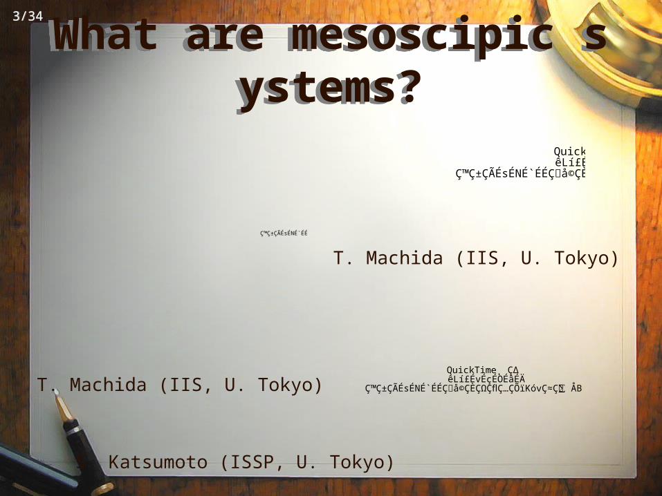
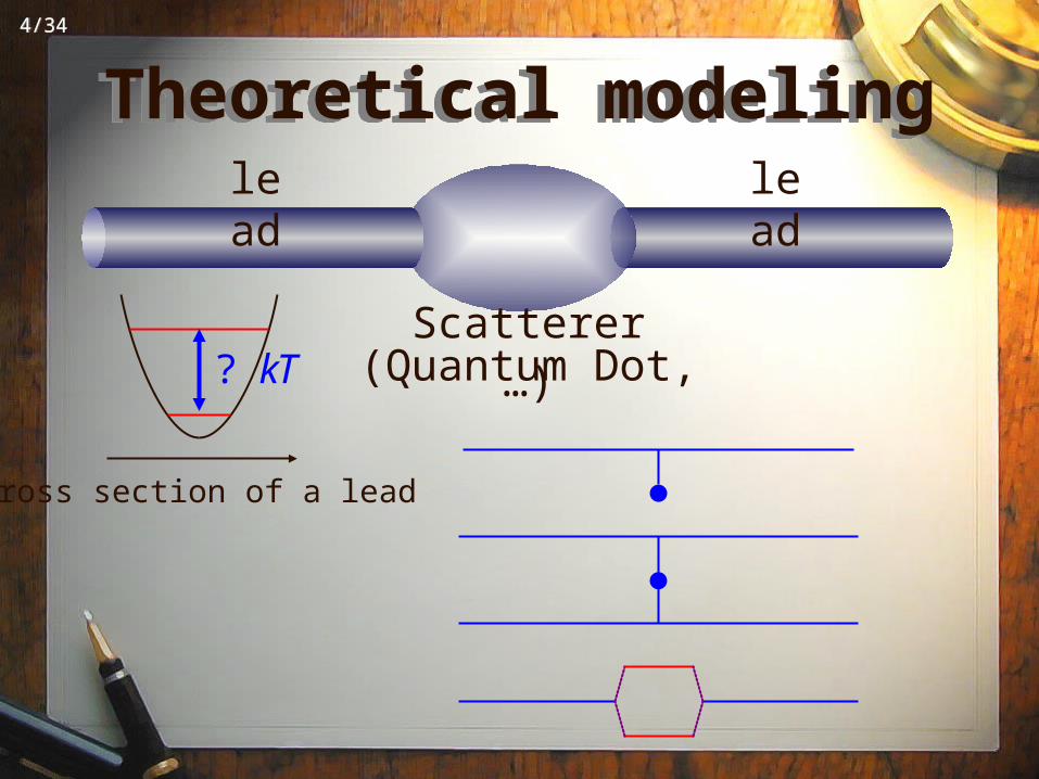
Theoretical modelingTheoretical modelinglead
Scatterer(Quantum Dot, …)
Cross section of a lead
lead
? kT
5/345/34
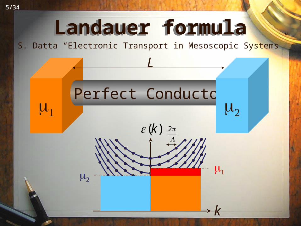
k
ε(k) 2πL
Landauer formulaLandauer formulaS. Datta “Electronic Transport in Mesoscopic Systems”
Perfect Conductor
L
6/346/34
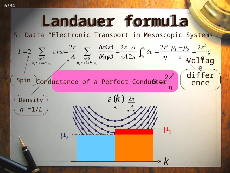
Landauer formulaLandauer formulaS. Datta “Electronic Transport in Mesoscopic Systems”
I = envv>0
<ε (k)<
∑ =eL
dε(k)d(hk)
=v>0
<ε (k)<
∑ ehL
Lπ
dε
∫ =e
h −
e=e
hV
k
ε(k)
2πL
G =e
hConductance of a Perfect ConductorSpin
Density
n =1/L
Voltage differenc
e
7/347/34
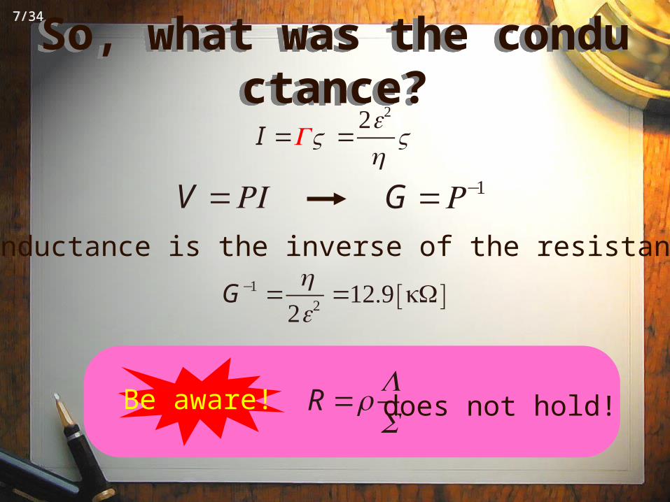
So, what was the conductance?So, what was the conductance?
I =GV =e
hV
V =RI G =R−
G− =he
=.9 kΩ[ ]
Conductance is the inverse of the resistance.
Be aware! R =ρLS does not hold!
8/348/34
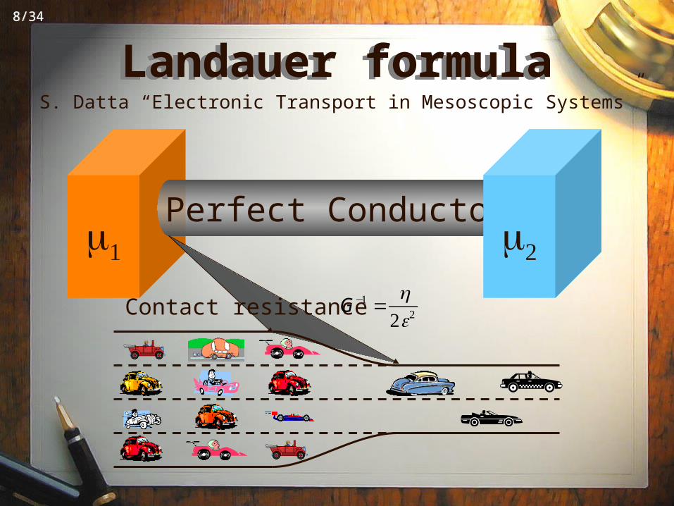
Perfect Conductor
Landauer formulaLandauer formulaS. Datta “Electronic Transport in Mesoscopic Systems”
Contact resistance G− =he
9/349/34
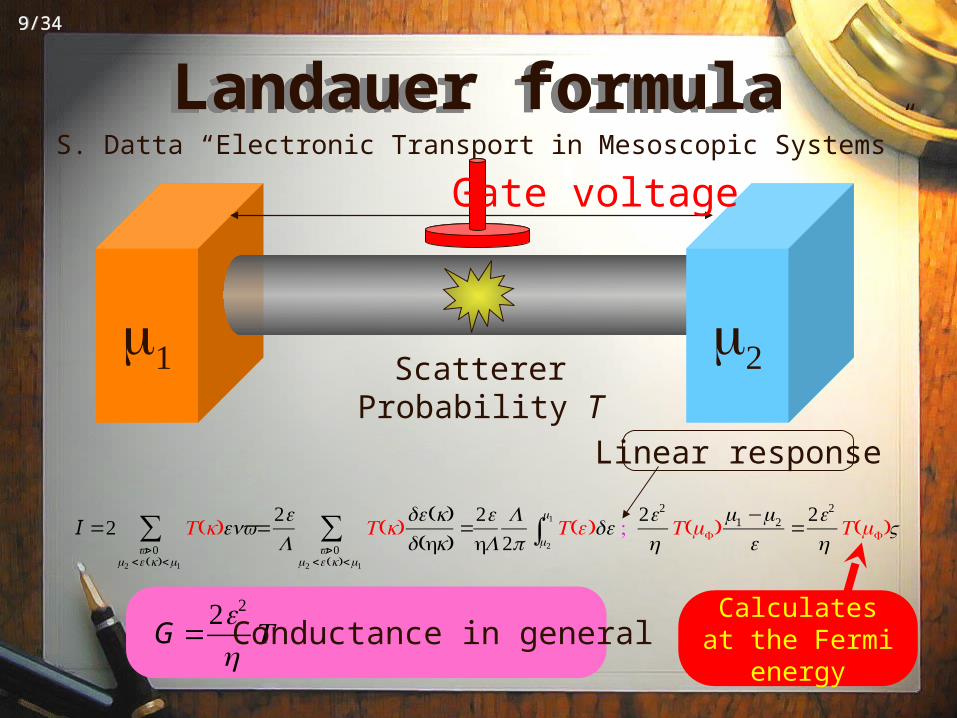
Landauer formulaLandauer formulaS. Datta “Electronic Transport in Mesoscopic Systems”
L
ScattererProbability T
I = T(k)envv>0
<ε (k)<
∑ =eL
T(k)dε(k)d(hk)
=v>0
<ε (k)<
∑ ehL
Lπ
T(ε)dε
∫ ;e
hT(F )
−e
=e
hT(F )V
G =e
hT Conductance in general
Linear response
Calculates at the Fermi energy
Gate voltage
10/3410/34
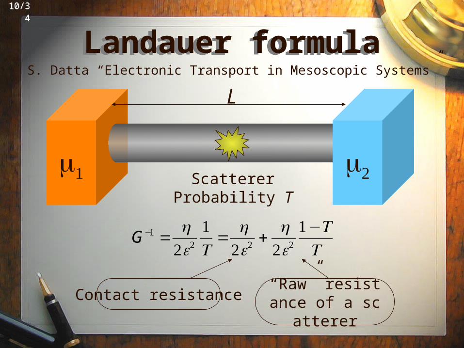
Landauer formulaLandauer formulaS. Datta “Electronic Transport in Mesoscopic Systems”
L
G− =he
T=
he+
he−T
T
Contact resistance “Raw” resistance of a scatterer
ScattererProbability T
11/3411/34
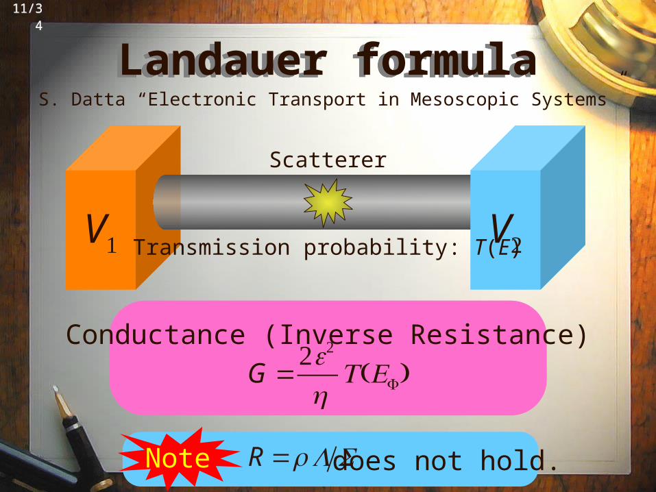
Landauer formulaLandauer formulaS. Datta “Electronic Transport in Mesoscopic Systems”
V VTransmission probability: T(E)
Scatterer
Conductance (Inverse Resistance)
G =e
hT(EF )
Note R =ρ L S does not hold.
12/3412/34
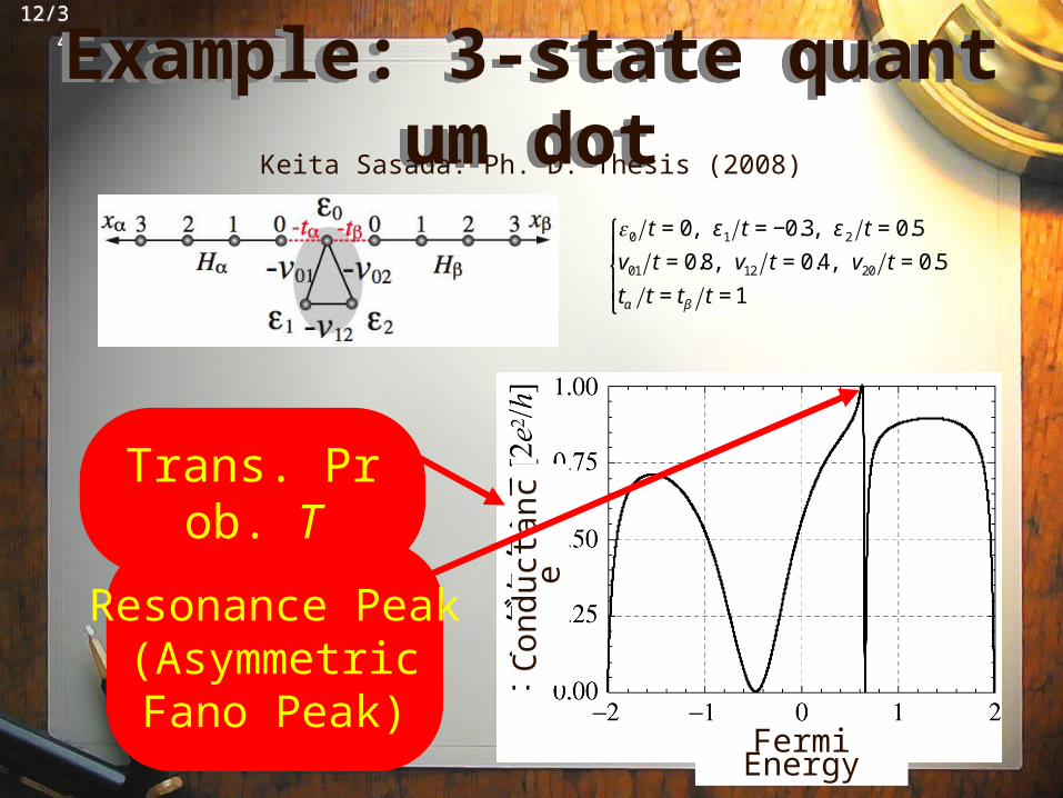
Example: 3-state quantum dotExample: 3-state quantum dotKeita Sasada: Ph. D. Thesis (2008)
ε0 t = 0, ε1 t = −0.3, ε 2 t = 0.5
v01 t = 0.8, v12 t = 0.4, v20 t = 0.5
tα t = tβ t = 1
⎧
⎨⎪
⎩⎪
Resonance Peak(AsymmetricFano Peak)
Trans. Prob. T
Fermi Energy
Con
duct
ance
13/3413/34
ContentsContents
1.Conductance and the Landauer Fo
rmula
2.Definition of Resonant States
3. Interference of Resonant States an
d the Fano Peak
14/3414/34
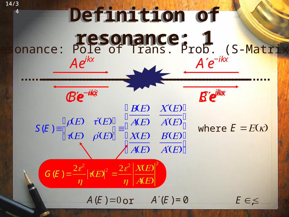
Definition of resonance: 1Definition of resonance: 1
Aeikx
CeikxBe−ikx
S(E)≡r(E) ′t (E)t(E) ′r (E)
⎛
⎝⎜
⎞
⎠⎟≡
B(E)A(E)
′C (E)′A (E)
C(E)A(E)
′B (E)′A (E)
⎛
⎝
⎜⎜⎜⎜
⎞
⎠
⎟⎟⎟⎟
′A e−ikx
′B eikx′C e−ikx
Pole → or , whereA(E)=0 ′A (E) = 0 E ∈£
where E =E(k)
Resonance: Pole of Trans. Prob. (S-Matrix)
G(E)=e
ht(E) =
e
hC(E)A(E)
15/3415/34
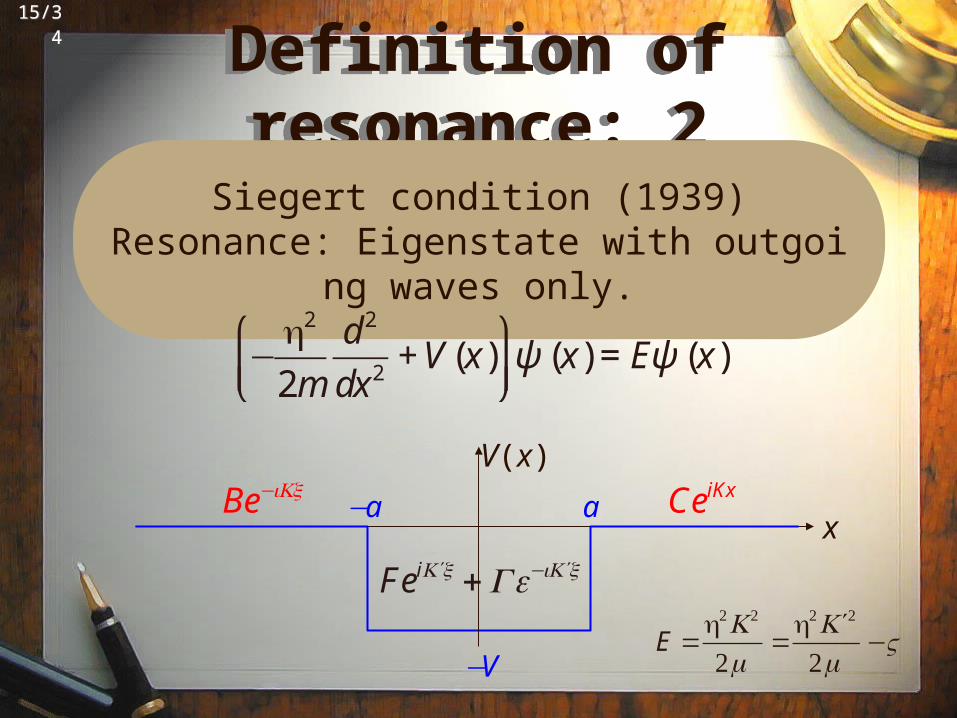
Definition of resonance: 2Definition of resonance: 2
Siegert condition (1939)Resonance: Eigenstate with outgoing waves only.
a−ax
Be−iKx CeiKx
−
h2
2m
d 2
dx2+ V (x)
⎛
⎝⎜⎞
⎠⎟ψ (x) = Eψ (x)
V(x)
−V
Fei ′K x +Ge−i ′K x
E =
hK
m=
h ′K
m−V
16/3416/34
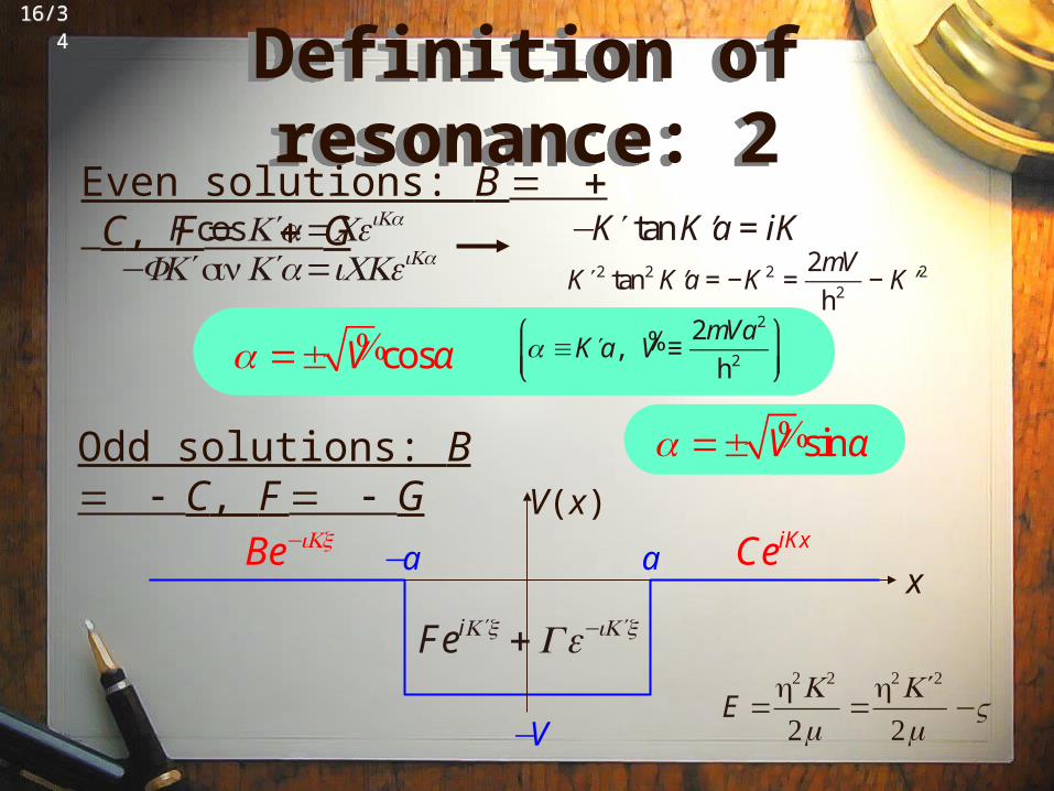
Definition of resonance: 2Definition of resonance: 2
a−ax
Be−iKx CeiKx
Fei ′K x +Ge−i ′K x
V(x)
−V
Even solutions: B C, F G
E =
hK
m=
h ′K
m−V
F cos ′K a=CeiKa
−F ′K sin ′K a=iCKeiKa
Odd solutions: B C, F G
− ′K tan ′K a = iK
′K 2 tan2 ′K a = −K 2 =
2mV
h2− ′K 2
α =± %V cosα
α =± %V sinα
α ≡ ′K a, %V ≡
2mVa2
h2
⎛
⎝⎜⎞
⎠⎟
17/3417/34
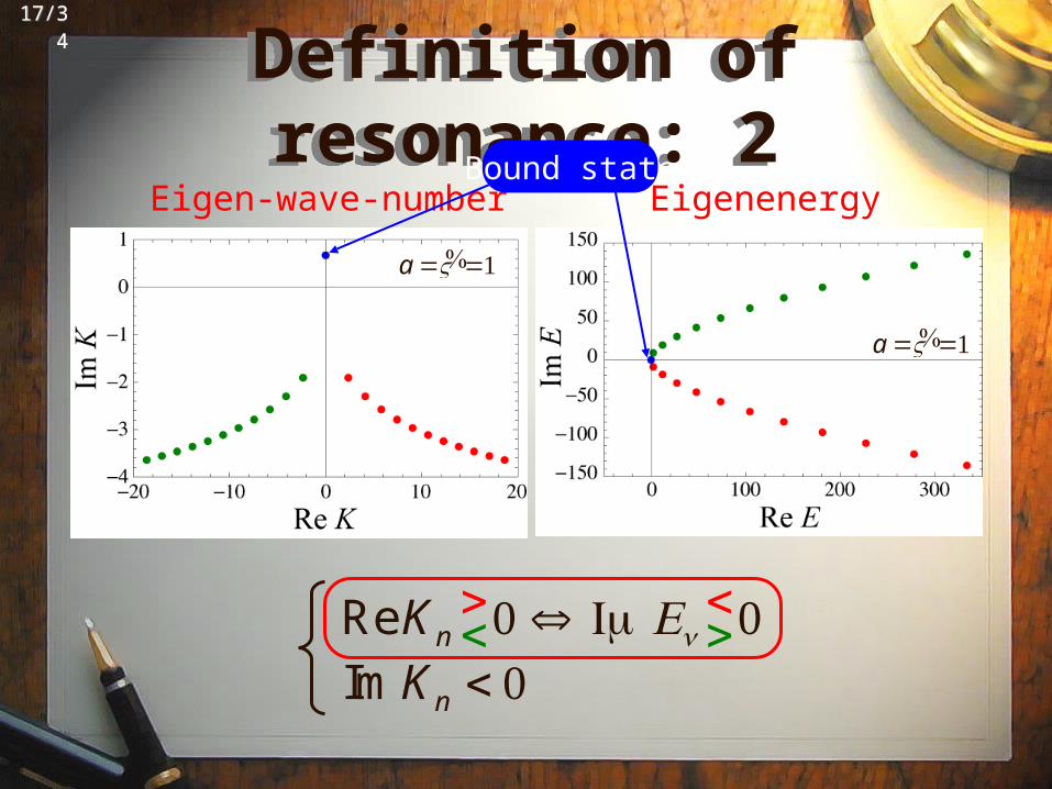
Definition of resonance: 2Definition of resonance: 2
Im Kn < 0Re Kn
><0 ⇔ ImEn
<>0
Eigen-wave-number EigenenergyBound state
a = %V =
a = %V =
18/3418/34
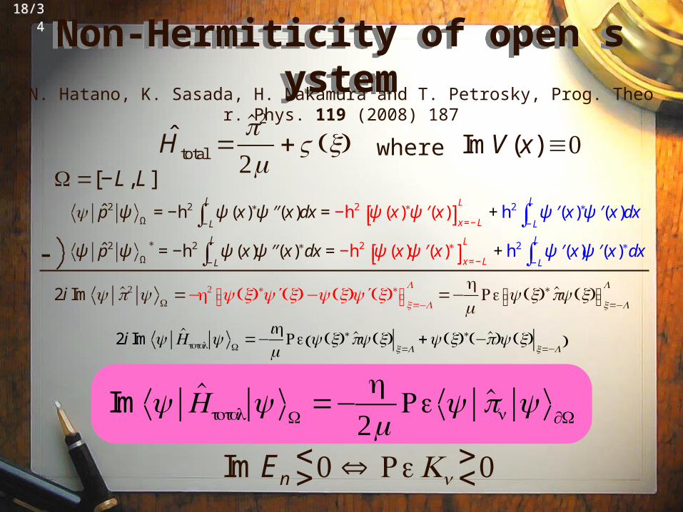
Non-Hermiticity of open systemNon-Hermiticity of open system
ψ p2 ψΩ
= −h2 ψ (x)∗ ′′ψ (x)dx− L
L
∫ = −h2 ψ (x)∗ ′ψ (x)⎡⎣ ⎤⎦x=− L
L+ h2 ′ψ (x)∗
− L
L
∫ ′ψ (x)dx
ψ p2 ψΩ
∗= −h2 ψ (x) ′′ψ (x)∗dx
− L
L
∫ = −h2 ψ (x) ′ψ (x)∗⎡⎣ ⎤⎦x=− L
L+ h2 ′ψ (x)
− L
L
∫ ′ψ (x)∗dx
2i Im ψ Htotal ψ Ω
=−ihm
Re ψ (x)∗pψ (x)x=L+ψ (x)∗(−p)ψ (x)
x=−L( )
Im ψ Htotal ψ Ω
=−hm
Reψ pn ψ ∂Ω
N. Hatano, K. Sasada, H. Nakamura and T. Petrosky, Prog. Theor. Phys. 119 (2008) 187
H total =p
m+V(x)
2i Im ψ p ψ
Ω=−h ψ (x)∗ ′ψ (x)−ψ (x) ′ψ (x)∗⎡⎣ ⎤⎦x=−L
L=−
hm
Re ψ (x)∗pψ (x)⎡⎣ ⎤⎦x=−L
L
where ImV (x)≡0
Im En<>0 ⇔ ReKn
><0
Ω=[−L, L]
19/3419/34
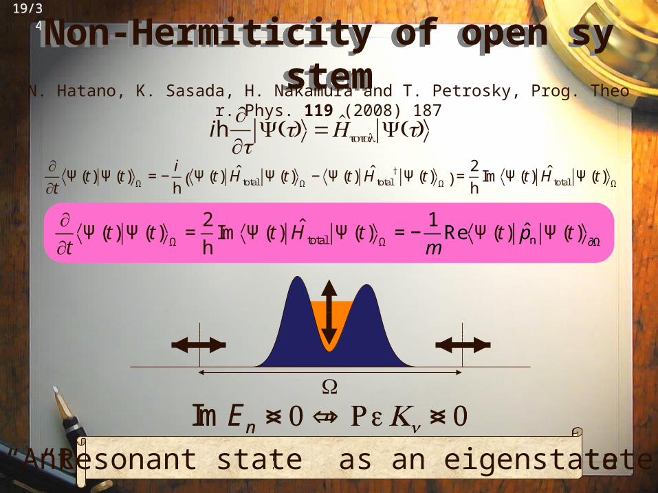
Non-Hermiticity of open systemNon-Hermiticity of open system
∂∂t
Ψ(t) Ψ(t)Ω
=2
hIm Ψ(t) H total Ψ(t)
Ω= −
1
mRe Ψ(t) pn Ψ(t)
∂Ω
N. Hatano, K. Sasada, H. Nakamura and T. Petrosky, Prog. Theor. Phys. 119 (2008) 187
Im En > 0 ⇔ ReKn < 0
ih∂∂tΨ(t) =Htotal Ψ(t)
∂∂t
Ψ(t) Ψ(t)Ω
= −i
hΨ(t) H total Ψ(t)
Ω− Ψ(t) H total
† Ψ(t)Ω( ) =
2
hIm Ψ(t) H total Ψ(t)
Ω
Im En < 0 ⇔ ReKn > 0Ω
“Anti-resonant state as an eigenstate“Resonant state” as an eigenstate
20/3420/34
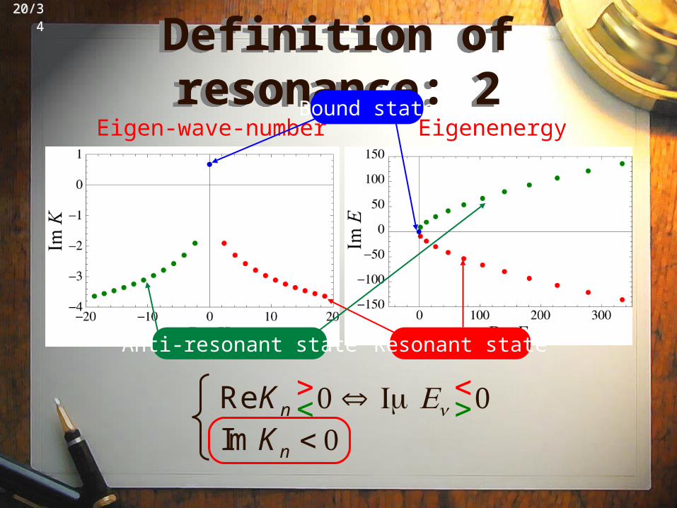
Definition of resonance: 2Definition of resonance: 2
Im Kn < 0Re Kn
><0 ⇔ ImEn
<>0
Eigen-wave-number EigenenergyBound state
Resonant stateAnti-resonant state
21/3421/34
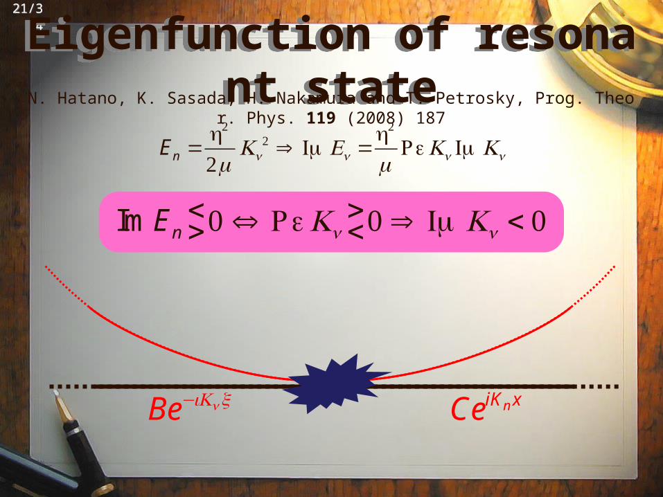
Eigenfunction of resonant stateEigenfunction of resonant stateN. Hatano, K. Sasada, H. Nakamura and T. Petrosky, Prog. Theor. Phys. 119 (2008) 187
Im En<>0 ⇔ ReKn
><0 ⇒ ImKn < 0
En =
h
mKn
⇒ ImEn =h
mReKn ImKn
CeiKn xBe−iKnx
22/3422/34
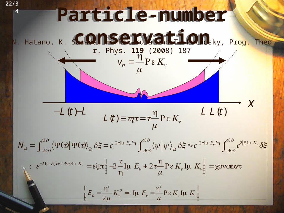
Particle-number conservationParticle-number conservationN. Hatano, K. Sasada, H. Nakamura and T. Petrosky, Prog. Theor. Phys. 119 (2008) 187
En =
h
mKn
⇒ ImEn =h
mReKn ImKn
⎛
⎝⎜⎞
⎠⎟
vn =
hm
ReKn
x
NΩ = Ψ(t) Ψ(t) Ω dx−L(t)
L(t)
∫ =e−t ImEn /h ψ ψΩ
dx−L(t)
L(t)
∫ ≈e−t ImEn /h e x ImKndx−L(t)
L(t)
∫: e− ImEnt+L(t) ImKn =exp −
th
ImEn + thm
ReKn ImKn⎛⎝⎜
⎞⎠⎟=constant
L−L L(t)−L(t)
L(t)≡vnt=t
hm
ReKn
23/3423/34
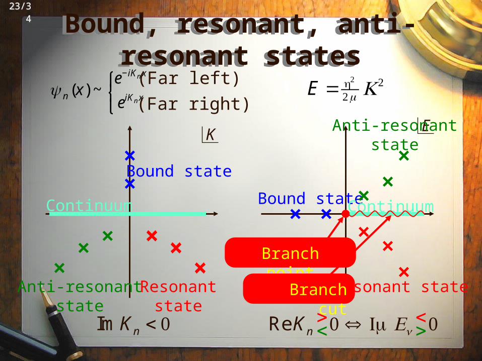
Bound, resonant, anti-resonant statesBound, resonant, anti-resonant states
K
Bound state
Resonantstate
Anti-resonantstate
Continuum
E
Bound state
Resonant state
Anti-resonantstate
Continuum
E =h
mK
Branch point
Branch cut
ψ n (x) ~e−iKn x
eiKn x
⎧⎨⎩
(Far left)
Im Kn < 0 Re Kn><0 ⇔ ImEn
<>0
(Far right)
24/3424/34
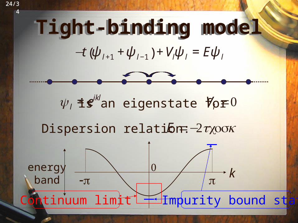
Tight-binding modelTight-binding model−t ψ l +1 +ψ l −1( ) + Vlψ l = Eψ l
Vl =0ψ l = eiklis an eigenstate for
E =−tcoskDispersion relation:
kππ0
Continuum limit Impurity bound state
energyband
25/3425/34
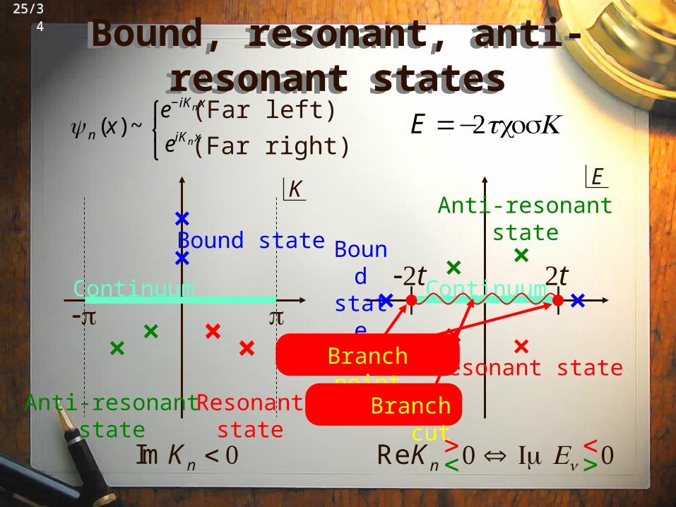
t t
Bound, resonant, anti-resonant statesBound, resonant, anti-resonant states
K
Bound state
Resonantstate
Anti-resonantstate
Continuum
E
Bound state
Resonant state
Anti-resonantstate
Continuum
E =−tcosK
Branch point
Branch cut
ψ n (x) ~e−iKn x
eiKn x
⎧⎨⎩
(Far left)
Im Kn < 0 Re Kn><0 ⇔ ImEn
<>0
(Far right)
π π
26/3426/34
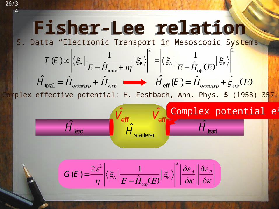
H leadH lead
Fisher-Lee relationFisher-Lee relation
T (E)∝ xL
E−H total + iη
xR
= xL
E−Heff (E)
xR
H eff (E)=Hscatterer + Veff (E)
H scatterer
H total =Hscatterer + H lead
Veff Veff
Complex effective potential: H. Feshbach, Ann. Phys. 5 (1958) 357
G(E)=e
hxL
E−Heff (E)
xR
dεL
dkdεR
dk
S. Datta “Electronic Transport in Mesoscopic Systems”
Complex potential eikx
27/3427/34
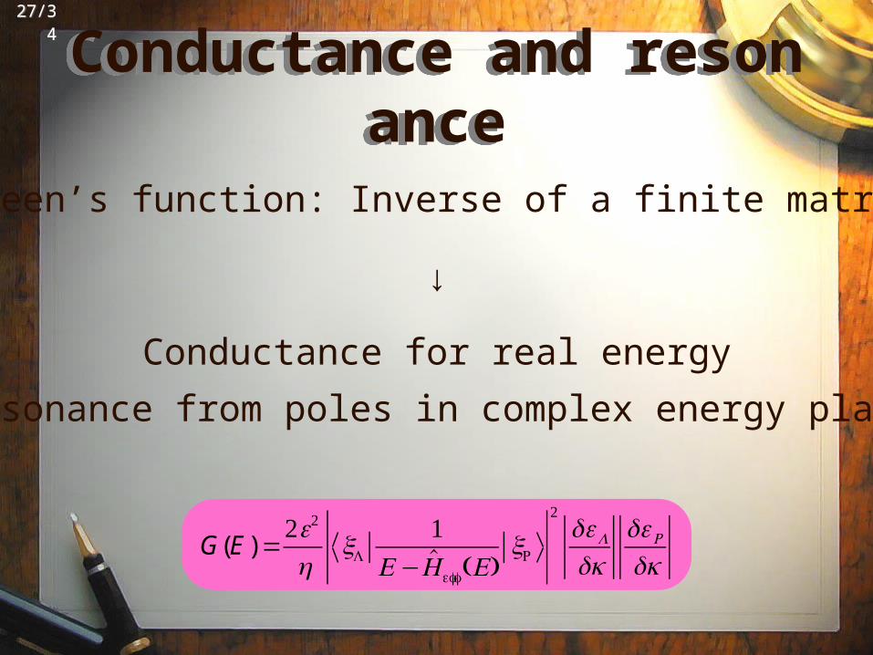
Conductance and resonanceConductance and resonance
G(E)=e
hxL
E−Heff (E)
xR
dεL
dkdεR
dk
Green’s function: Inverse of a finite matrix
↓
Conductance for real energy
Resonance from poles in complex energy plane

28/3428/34
ContentsContents
1.Conductance and the Landauer Fo
rmula
2.Definition of Resonant States
3. Interference of Resonant States an
d the Fano Peak
29/3429/34
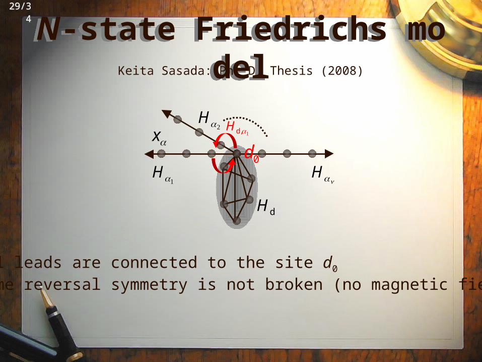
N-state Friedrichs modelN-state Friedrichs model
xα
Hα
Hd,α
Hd
Hα
Hαn
d0
Keita Sasada: Ph. D. Thesis (2008)
• All leads are connected to the site d0
• Time reversal symmetry is not broken (no magnetic field)
30/3430/34
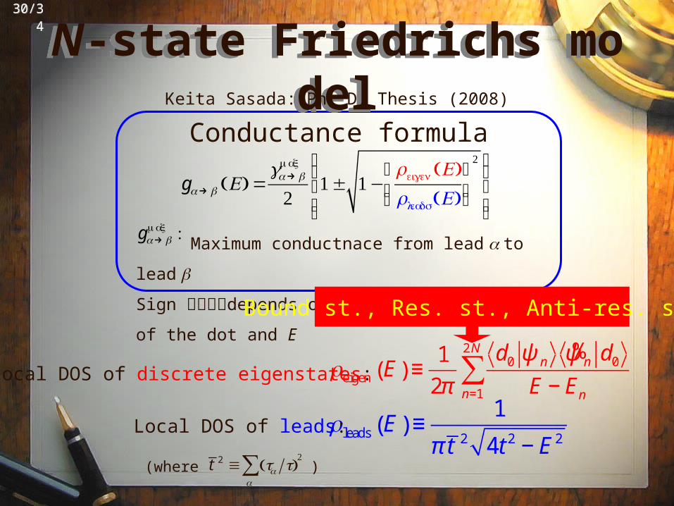
Conductance formula
N-state Friedrichs modelN-state Friedrichs model
ρleads E( ) ≡1
π t 2 4t 2 − E2
Local DOS of discrete eigenstates:
gα→ β E( ) =gα→ β
max
± −
ρeigen E( )ρleads E( )
⎛
⎝⎜⎞
⎠⎟
⎧⎨⎪
⎩⎪
⎫⎬⎪
⎭⎪
ρeigen E( ) ≡
1
2π
d0 ψ n%ψ n d0
E − Enn=1
2 N
∑
Local DOS of leads:
Maximum conductnace from lead α to lead β
Sign depends on the inner structure of the dot and
E
gα→ βmax :
t 2 ≡ tα t( )
α∑(where )
Bound st., Res. st., Anti-res. st.
Keita Sasada: Ph. D. Thesis (2008)
31/3431/34
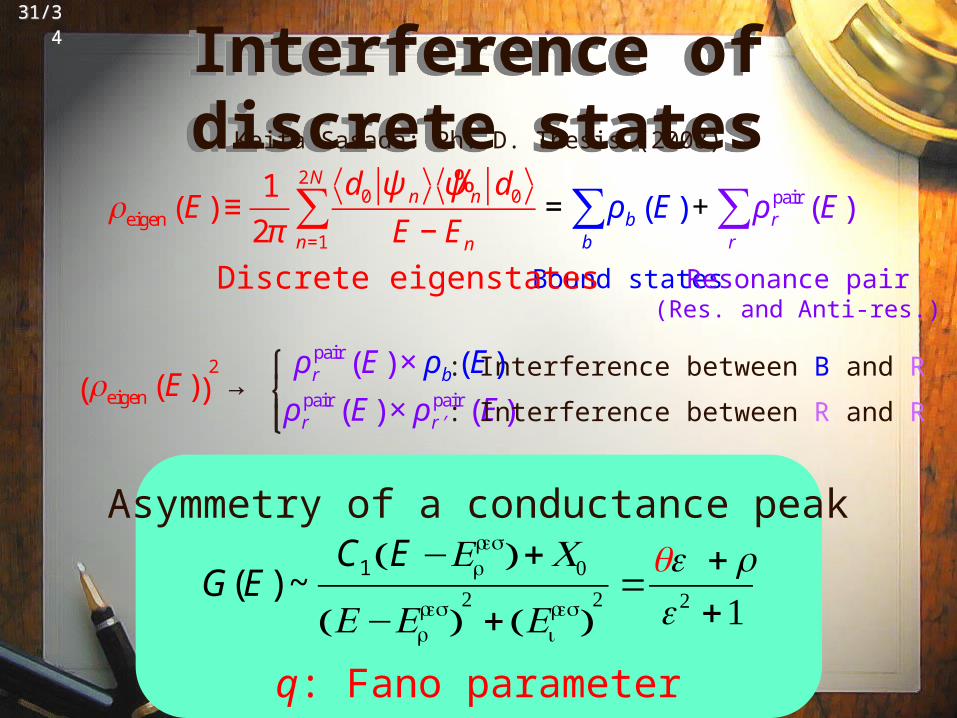
Interference of discrete statesInterference of discrete states
Bound states Resonance pair(Res. and Anti-res.)
: Interference between B and R
ρeigen E( ) ≡
1
2π
d0 ψ n%ψ n d0
E − Enn=1
2 N
∑ = ρb E( )b
∑ + ρ rpair E( )
r∑
Keita Sasada: Ph. D. Thesis (2008)
Discrete eigenstates
G(E) ~C1 E −Er
res( ) +C0
E−Erres( )
+ Ei
res( ) =
qε + rε +
Asymmetry of a conductance peak
q: Fano parameter
ρeigen E( )( )2
→ρ r
pair E( ) × ρb E( )
ρ rpair E( ) × ρ ′r
pair E( )
⎧⎨⎩⎪ : Interference between R and R
32/3432/34
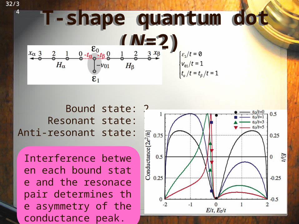
T-shape quantum dot (N=2) T-shape quantum dot (N=2)ε1 t = 0
v01 t = 1
tα t = tβ t = 1
⎧
⎨⎪
⎩⎪
Bound state: 2 Resonant state: 1
Anti-resonant state: 1
Interference between each bound state and the resonace pair determines the asymmetry of the conductance peak.
Bound state 1 Bound state 2
Anti-resonant state
Resonant state
33/3433/34
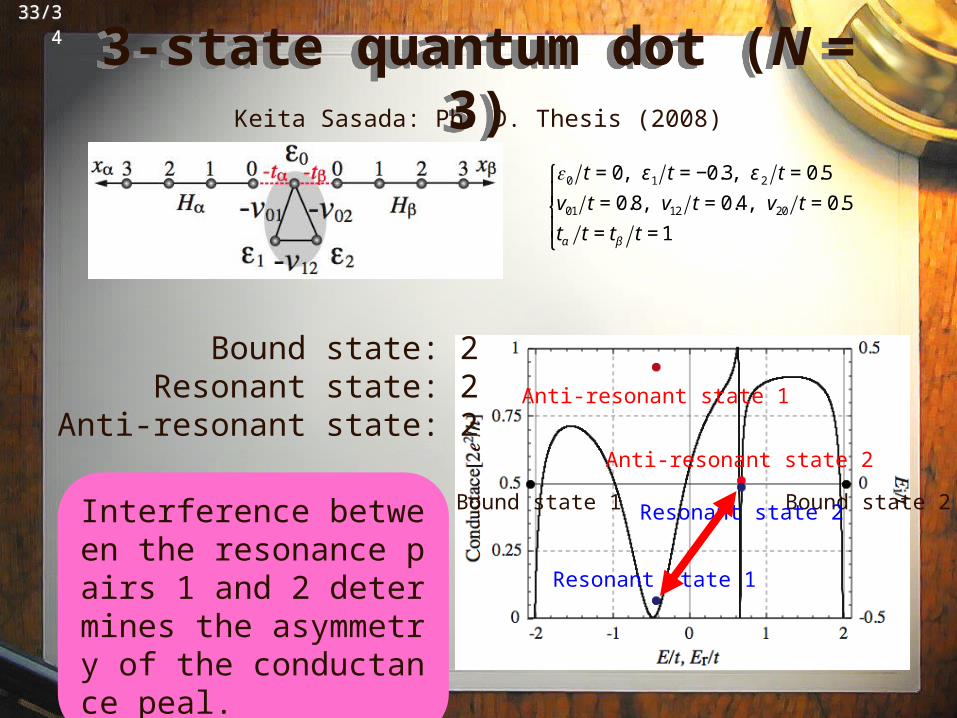
3-state quantum dot (N = 3)3-state quantum dot (N = 3)Keita Sasada: Ph. D. Thesis (2008)
ε0 t = 0, ε1 t = −0.3, ε 2 t = 0.5
v01 t = 0.8, v12 t = 0.4, v20 t = 0.5
tα t = tβ t = 1
⎧
⎨⎪
⎩⎪
Bound state 1 Bound state 2
Anti-resonant state 2
Anti-resonant state 1
Resonant state 1
Resonant state 2Interference between the resonance pairs 1 and 2 determines the asymmetry of the conductance peal.
Bound state: 2 Resonant state: 2
Anti-resonant state: 2
34/3434/34
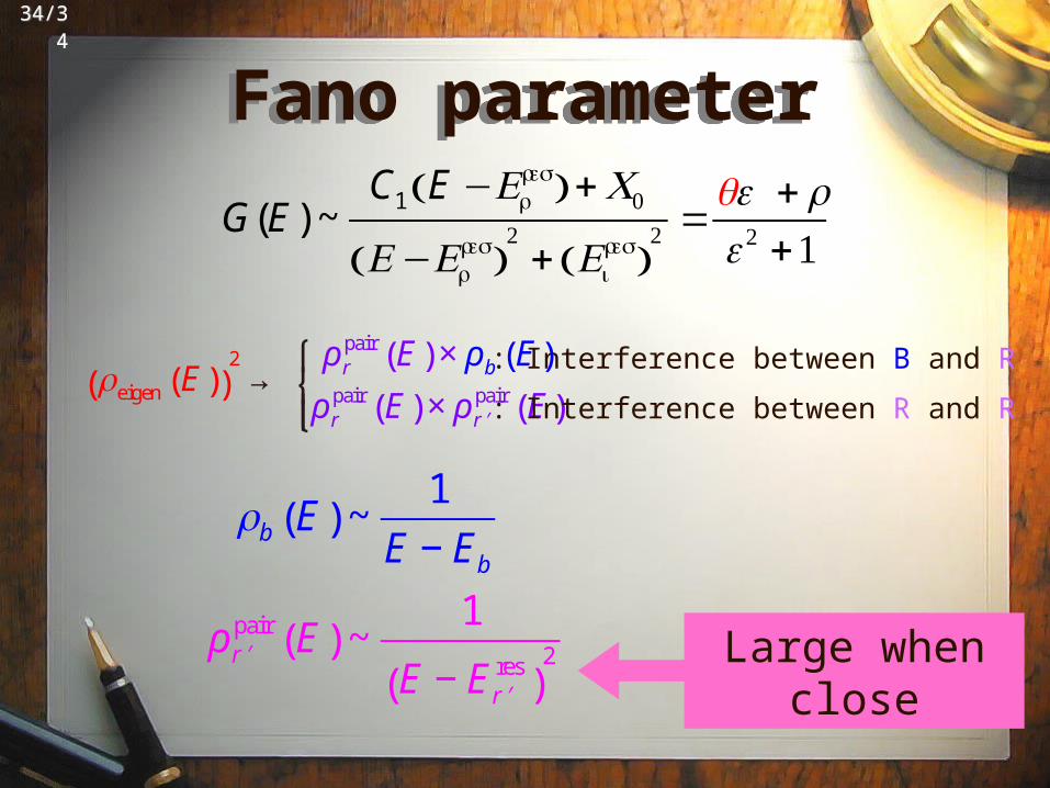
Fano parameterFano parameter
ρb E( ) ~1
E − Eb
ρ ′rpair E( ) ~
1
E − E ′rres( )
2
G(E) ~C1 E −Er
res( ) +C0
E−Erres( )
+ Ei
res( ) =
qε + rε +
Large when close
: Interference between B and Rρeigen E( )( )2
→ρ r
pair E( ) × ρb E( )
ρ rpair E( ) × ρ ′r
pair E( )
⎧⎨⎩⎪ : Interference between R and R
35/3435/34
SummarySummary
- Electronic conduction and resonance scattering
- Definition and physics of resonant states
- Particle-number conservation
- Interference between resonant states
36/3436/34
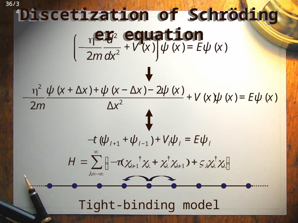
Discetization of Schrödinger equationDiscetization of Schrödinger equation
−
h2
2m
d 2
dx2+ V (x)
⎛
⎝⎜⎞
⎠⎟ψ (x) = Eψ (x)
−
h2
2m
ψ (x + Δx) + ψ (x − Δx) − 2ψ (x)
Δx2+ V (x)ψ (x) = Eψ (x)
−t ψ l +1 +ψ l −1( ) + Vlψ l = Eψ l
H = −t cl+†cl + cl
†cl+( ) +Vlcl†cl⎡⎣ ⎤⎦
l=−∞
∞
∑
Tight-binding model