Methodology for diagnosing of skin cancer on images of ...usuario.cicese.mx/~josue/pdf/biomedical_optics_express_2015.pdf · Methodology for diagnosing of skin cancer on images of

Methodology for diagnosing of skin cancer on images of dermatologic spots by spectral analysis

Esperanza Guerra-Rosas1,2 and Josué Álvarez-Borrego3,4 1Departamento de Investigación en Física, Universidad de Sonora (UNISON), Luis Encinas y Rosales S/N, Col.

Centro, Hermosillo, Sonora, C.P. 83000, Mexico [email protected]

3Centro de Investigación Científica y de Educación Superior de Ensenada (CICESE), División de Física Aplicada, Departamento de Óptica, Carretera Ensenada-Tijuana No. 3918, Fraccionamiento Zona Playitas, Ensenada, Baja

California, C.P. 22860, Mexico [email protected]

Abstract: In this paper a new methodology for the diagnosing of skin cancer on images of dermatologic spots using image processing is presented. Currently skin cancer is one of the most frequent diseases in humans. This methodology is based on Fourier spectral analysis by using filters such as the classic, inverse and k-law nonlinear. The sample images were obtained by a medical specialist and a new spectral technique is developed to obtain a quantitative measurement of the complex pattern found in cancerous skin spots. Finally a spectral index is calculated to obtain a range of spectral indices defined for skin cancer. Our results show a confidence level of 95.4%.

©2015 Optical Society of America

OCIS codes: (100.2000) Digital image processing, (070.2615) Frequency filtering.

References and links

1. M. J. Eide, M. M. Asgari, S. W. Fletcher, A. C. Geller, A. C. Halpern, W. R. Shaikh, L. Li, G. L. Alexander, A. Altschuler, S. W. Dusza, A. A. Marghoob, E. A. Quigley, and M. A. Weinstock; Informed (Internet course for Melanoma Early Detection) Group, “Effects on skills and practice from a web-based skin cancer course for primary care providers,” J. Am. Board Fam. Med. 26(6), 648–657 (2013).

2. American Cancer Society. Cancer Facts and Figs. (2014). 3. N. R. Telfer, G. B. Colver, and C. A. Morton; British Association of Dermatologists, “Guidelines for the

management of basal cell carcinoma,” Br. J. Dermatol. 159(1), 35–48 (2008). 4. A. Kricker, B. Armstrong, V. Hansen, A. Watson, G. Singh-Khaira, C. Lecathelinais, C. Goumas, and A. Girgis,

“Basal cell carcinoma and squamous cell carcinoma growth rates and determinants of size in community patients,” J. Am. Acad. Dermatol. 70(3), 456–464 (2014).

5. E. A. Gordon Spratt and J. A. Carucci, “Skin cancer in immunosuppressed patients,” Facial Plast. Surg. 29(5), 402–410 (2013).

6. S. Ogden and N. R. Telfer, “Skin cancer,” Medicine (Baltimore) 37(6), 305–308 (2009). 7. K. Korotkov and R. Garcia, “Computerized analysis of pigmented skin lesions: a review,” Artif. Intell. Med.

56(2), 69–90 (2012). 8. A. O. Berg, D. Best; US Preventive Services Task Force, “Screening for Skin Cancer: recommendations and

rationale,” Am. J. Prev. Med. 20(3 Suppl), 44–46 (2001). 9. M. M. Rahman and P. Bhattacharya, “An integrated and interactive decision support system for automated

melanoma recognition of dermoscopic images,” Comput. Med. Imaging Graph. 34(6), 479–486 (2010). 10. A. G. Isasi, B. G. Zapirain, and A. M. Zorrilla, “Melanomas non-invasive diagnosis application based on the

ABCD rule and pattern recognition image processing algorithms,” Comput. Biol. Med. 41(9), 742–755 (2011). 11. P. G. Cavalcanti and J. Scharcanski, “Automated prescreening of pigmented skin lesions using standard

cameras,” Comput. Med. Imaging Graph. 35(6), 481–491 (2011). 12. J. A. Jaleel, S. Salim, and R. B. Aswin, “Artificial neural network based detection of skin cancer,” IJAREEIE 1,

200–205 (2012). 13. M. Sadeghi, M. Razmara, T. K. Lee, and M. S. Atkins, “A novel method for detection of pigment network in

dermoscopic images using graphs,” Comput. Med. Imaging Graph. 35(2), 137–143 (2011). 14. C. Barata, J. S. Marques, and J. Rozeira, “A system for the detection of pigment network in dermoscopy images

using directional filters,” IEEE Trans. Biomed. Eng. 59(10), 2744–2754 (2012).

#242232 Received 8 Jun 2015; revised 21 Jul 2015; accepted 24 Aug 2015; published 9 Sep 2015 (C) 2015 OSA 1 Oct 2015 | Vol. 6, No. 10 | DOI:10.1364/BOE.6.003876 | BIOMEDICAL OPTICS EXPRESS 3876

15. G. Betta, G. Di Leo, G. Fabbrocini, A. Paolillo, and P. Sommella, “Dermoscopic image-analysis system: Estimation of atypical pigment network and atypical vascular pattern,” presented at the International Workshop on Medical Measurement and Applications, Benevento, Italy, 20–21 April 2006.

16. M. E. Celebi, H. A. Kingravi, B. Uddin, H. Iyatomi, Y. A. Aslandogan, W. V. Stoecker, and R. H. Moss, “A methodological approach to the classification of dermoscopy images,” Comput. Med. Imaging Graph. 31(6), 362–373 (2007).

17. N. Smaoui and S. Bessassi, “A developed system for melanoma diagnosis,” Int. J. Comput. Vis. 3(1), 10–17 (2013).

18. J. Premaladha and K. S. Ravichandran, “Asymmetry analysis of malignant melanoma using image processing: a survey,” Science Alert 7(2), 45–53 (2014).

19. E. Guerra-Rosas, J. Álvarez-Borrego, and Á. Coronel-Beltrán, “Diagnosis of skin cancer ussing image processing,” Proceedings of AIP Conference 1618, 155 (2014).

20. S. Uchida, “Image processing and recognition for biological images,” Dev. Growth Differ. 55(4), 523–549 (2013).

21. A. B. Vander Lugt, “Signal detection by complex spatial filtering,” IEEE Trans. Inf. Theory 10(2), 139–145 (1964).

22. A. A. S. Awwal, M. A. Karim, and S. R. Jahan, “Improved correlation discrimination using an amplitude-modulated phase-only filter,” Appl. Opt. 29(2), 233–236 (1990).

23. B. V. K. V. Kumar and L. Hassebrook, “Performance measures for correlation filters,” Appl. Opt. 29(20), 2997–3006 (1990).

24. R. E. Guerrero and J. Álvarez Borrego, “Nonlinear composite filter performance,” Opt. Eng. 48(6), 067021 (2009).

25. M. A. Bueno-Ibarra, M. C. Chávez-Sánchez, and J. Álvarez-Borrego, “Nonlinear law spectral technique to analyze white spot syndrome virus infection,” IJALS 2(3,4), 125–132 (2010).

1. Introduction

Skin cancer is one of the diseases that affect humans. It is caused by the development of cancerous cells on any of the layers of skin and occurs when cells in a body part begin to grow out of control and spread to other organs and tissues. United States is one of the countries that has had greater incidence of this disease and represents an important health problem. There are three major types of skin cancer which are basal cell carcinoma, squamous cell carcinoma and melanoma [1, 2]. Basal cell carcinoma is the most common skin cancer, however is the least dangerous if it is detected early. This cancer appears in cells that are in the deeper layers of skin, usually in parts of the body that are exposed to the sun such as the face, head, neck, ears, shoulders and back, however occurs most often in the face, this type rarely causes a metastasis [3–6]. Squamous cell carcinoma is the second most common type of skin cancer, which appears in the cells that make up the upper skin layers, it is more likely to spread to areas under the skin. It is usually found on parts of the body that are exposed to uv light, therefore it can appear on legs or feet, it can be locally invasive, it may be able to reach large sizes if is not detected early. It is able to cause metastasis [6], classically it is presented as a nodule, papule or tumor [5]. Melanoma is the least common compared to other types, but is the most dangerous because it can cause death if is not detected early. It is able to take place anywhere on the skin, but is more likely to develop in certain locations. Like basal cell and squamous cell cancers, melanoma is almost always curable in its early stages [6, 7].

Skin cancer is very common in Europe, Australia and USA [6] and is almost always curable if recognized and treated early. The major risk factors related are skin color, sun exposure, climate, advanced age, genetic and familial history. The best way to detect melanoma is to recognize a new spot in the skin or a spot that is changing in size, shape and color. Early detection of skin cancer can avoid death [8].

Currently this disease represents a serious health problem, the search for an accurate clinical diagnosis has been a constant concern for dermatologists. Nowadays some methodologies on the area of image processing have been developed using algorithms or systems for detection and classification by means of techniques and computational methods, which have been applied in solving medical problems. These methodologies can be a very effective tool especially where there are not specialists, on other hand it is also a noninvasive tool for the patient [7–9]. Over the last decades image processing has been applied in different


areas, allowing to improve the information on an image for its interpretation, representation, description, and processing.

In the last years several studies and works related with images of pigmented skin lesions for diagnosis and classifying skin lesion such as skin cancer have been developed by means of digital images analysis. Their main objective have been to provide an accurate diagnosis. Most studies are related to the diagnosis of malignant melanoma. Gola et al. [10] developed an automated dermatological tool to identify melanoma. Their algorithms are based on identifying three categories: reticular, globular and homogeneous blue pigmentation. An important aspect of their work is to extract the shape of the skin lesion and then extract features of interest. Each algorithm cannot make a final decision therefore they will develop a system correlating all algorithms in order to perform a correct diagnosis. Rahman and Bhattacharya [9] proposed a similar method to recognize melanoma malignant. They presented a decision system using different classifiers such as support vector machine (SVMs), k-nearest neighbors (K-NNs) and Gaussian maximum likelihood (G-ML). The morphology of the lesion is detected applying a thresholding-based segmentation method then the lesion mask is obtained which contains the area of the lesion in the grey level. Color features are extracted from the lesion mask to train the respective classifiers after a comparison of single classifiers are performed, where the highest percentage of precision obtained with one of the classifiers was 72.45%. In their method melanoma, benign lesions and dysplastic nevi were classified. Cavalcanti and Scharcanski [11] proposed a method for classifying pigmented skin lesions as benign or malignant using two classifiers: the k-nearest neighbors (KNN) and the KNN followed by a Decision three (KNN-DT). First a preprocessing is applied to the image where shading effects are attenuated, for this the original image of the RGB color space is converted to HSV color space. Then a segmentation method is developed considering texture and color patterns of the image, in this step some operation are applied to eliminate imperfections caused by noise. Of the segmented image a set of features is extracted according to the ABCD rule (i.e., asymmetry, border irregularity color variation and diameter). Both classifiers were trained with these features. The result showed an accuracy of 94.54% to predict a lesion as benign or malignant. The methodology proposed by Jaleel et al. [12] is based on image processing techniques using Artificial Neuronal Network. Their main objective was classify melanoma from other skin diseases. The image was preprocessed in order to remove the noise present in it. Then it is smoothed by the median filter. After the image is segmented and binarized using threshold segmentation. 2D wavelet transform is applied over the segmented image to extract the features such as mean, standard deviation, absolute mean, L1 norm and L2 norm. The network was trained with features. Therefore its accuracy rate is good however it can be improved for this system. Given a dermoscopic image Sadegui et al. [13] classified the absence or presence of a pigmented network. First the image was preprocessed applying a high-pass filter to remove the low-frequency noise. This step was made on different color transformations (NTSC, L*a*b*, red, green and blue). A Laplacian of Gaussian filter (LoG) was applied in order to find meshes or cyclic structures, which represent the presence of a pigmented network region. The set of subgraphs obtained is converted to a graph using an eight connected components analysis, after noise or unwanted structures are removed. Considering distance between nodes corresponding to a hole found in each subgraph a high-level graph is created. By mean of this graph is obtained the density ratio, which compares the number of edges in the graph with its vertices and the entire lesion area. Density is used to detect a pigmented network. They reported a percentage of classification of 94.3%. Barata et al. [14] proposed a system for detecting a pigmented network. This method uses directional filters. The image is converted in grayscale to remove hair and reflections caused by the dermoscopy gel. The intensity property is taken to enhance the pigment network applying directional filters and geometry or spatial organization is used to generate a binary net-mask. Therefore spatial organization is carried out whit the connection of all pixels. Then a label is assigned to each binary image


that is with or without pigmented network. Features are extracted and used to train a classifier using the boosting algorithm. The algorithm was tested on a data set of 200 dermoscopy image (88 with pigment network and 112 without). They reported results of 82.1% for the classification. Betta et al. [15] described a method for detecting a typical pigmented network. This methodology is based on the combination of structural and spectral technique. The structural technique is made to identify the texture defined by local discontinuities such as lines and/or points. This is obtained by comparing the monochromatic image with the image which applied median filter. The spectral technique is based on the Fourier analysis of the image to obtain the spatial period of texture in this way a “regions with network” mask is created. Therefore this mask joins with segmented mask obtaining a “network image”, where the lesion area and pigment network are highlight. Finally to quantify the nature of the network two indices related to the spatial and chromatic variability have been obtained. To evaluate the performance of this method 30 images were evaluated.

The majority of the studies published in the literature such as [16–18] include similar stages as in the works mentioned above. These methods consists, generally of four stages which are: (i) acquire de image set, (ii) segmentation (which include several methods i.e techniques based on edges, thresholding, histogram segmentation, region growing, etc.), (iii) feature extraction (iv) classification or detection of a lesion for diagnosis.

It is important to evaluate patients with spotted skin quickly and efficiently through a noninvasive technique easy to implement. The importance of obtaining an accurate diagnostic method has led to develop techniques based on image processing

The aim of this work has been to develop a new methodology for diagnosing skin cancer based on images processing techniques applying different techniques of Fourier spectral filtering such as classic, inverse and k-law nonlinear [19].

Fourier spectral analysis techniques have demonstrated the capability to analyze important features from images in several fields being one of the most powerful tools.

2. Materials and methods

2.1 Image acquisition and construction of image bank

The image bank was created with images of skin cancer provided by the Dermatology Department of Centenario Hospital Hidalgo and the Instituto Nacional de Cancerología (INcan) in Mexico City. The images were classified as basal cell carcinoma, squamous cell carcinoma and melanoma by certified dermatologists after histopathological examination. Some images are shown in Fig. 1.


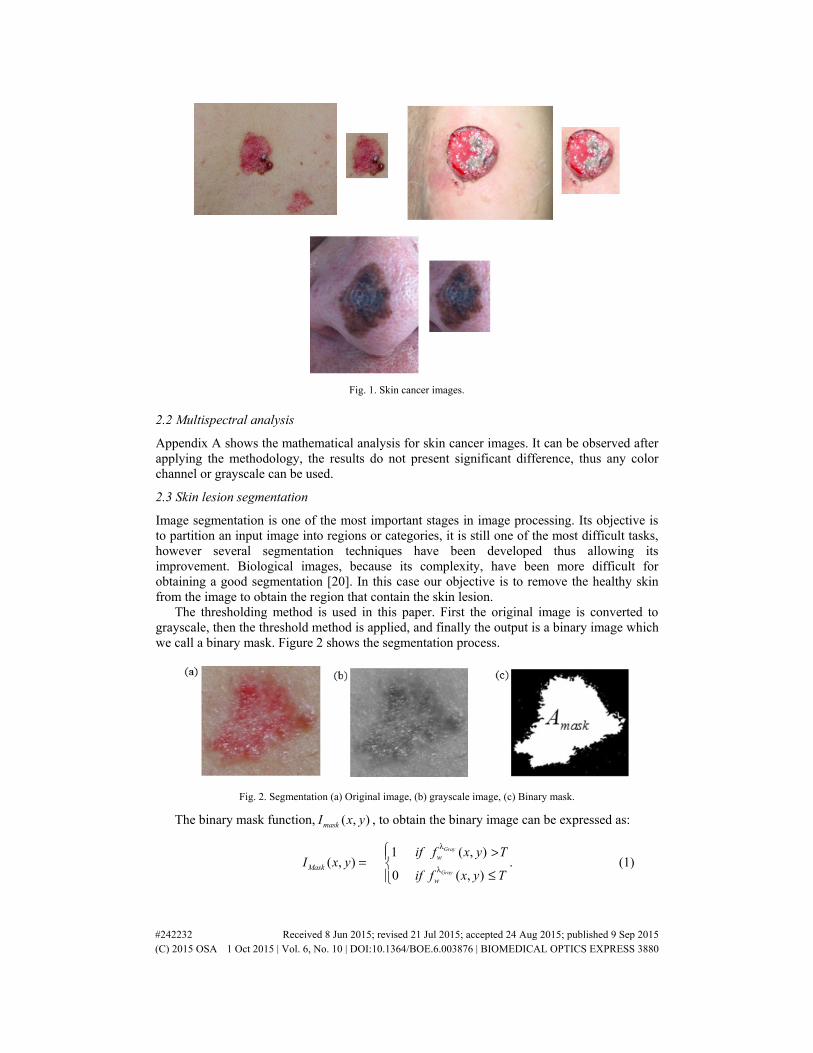
Fig. 1. Skin cancer images.

2.2 Multispectral analysis

Appendix A shows the mathematical analysis for skin cancer images. It can be observed after applying the methodology, the results do not present significant difference, thus any color channel or grayscale can be used.

2.3 Skin lesion segmentation

Image segmentation is one of the most important stages in image processing. Its objective is to partition an input image into regions or categories, it is still one of the most difficult tasks, however several segmentation techniques have been developed thus allowing its improvement. Biological images, because its complexity, have been more difficult for obtaining a good segmentation [20]. In this case our objective is to remove the healthy skin from the image to obtain the region that contain the skin lesion.

The thresholding method is used in this paper. First the original image is converted to grayscale, then the threshold method is applied, and finally the output is a binary image which we call a binary mask. Figure 2 shows the segmentation process.

Fig. 2. Segmentation (a) Original image, (b) grayscale image, (c) Binary mask.

The binary mask function, ( , )maskI x y , to obtain the binary image can be expressed as:

1 ( , )

( , ) .0 ( , )

Gray

Gray

wMask

w

if f x y TI x y

if f x y T

λ

λ

>= ≤

(1)


Where T is a threshold value and x, y are the coordinates of the threshold value point. Then all the gray level values greater than T will be classified as white taking the value 1, and all values less than or equal to T will be black taking the value 0. Finally, in order to do the binary mask the values are interchanged, of this way the interest area is filled with ones.

To avoid problems when determining the threshold value, the Otsu method was used which provides the optimal threshold value under the criterion of maximum variance between the background and the object. This can be expressed by

2( ).T max= σ (2)

The function maskA contains the total area of binary mask over the region of interest to

analyze, given by:

,

( , ), 0.mask Mask Maskx y

A I x y for I= > (3)

The intensity matrix data of the selected channel are bitwise multiplied by the binary mask

function ( ),MaskI x y , obtaining the function ( , )cwI x yλ which contains the information of

interest of the spot that will be analyzed, thus ( , ) ( , ) ( , )ccw w MaskI x y f x y I x y

λλ = where the

symbol represents a multiplication.

2.4 Sub-images

The binary image was divided into twenty five sub-images ( , )MaskI x y , where each sub-image

jMaskA has its respective area, ( 1,..., 25t hj = ). The sub-images are show in Fig. 3.

Fig. 3. Sub-images jmaskI of the binary mask.

Moreover, the image of the function ( , )cwI x yλ is divided into twenty five sub-images as

shown in Fig. 4 each sub-image is represented by the corresponding function ( , ).c

jwI x yλ


Fig. 4. Sub-images 1, ..., 25( , ),c t h

jw jI x yλ = .

The sub-image ( , )c

jwI x yλ is selected under the condition 1

3( , ) ,

j jMask MaskA I x y ≥ in

order to select only sub-images that contain information greater than or equal to one third of the total area of the sub-image. Figure 5 shows the sub-images that meet the condition for this case.

Fig. 5. Sub-image ( , )c

jwI x yλ with information greater than or equal to one third of the area.


2.5 Digital filters (spatial filters)

Appendix B gives us a complete description of the three spatial filters used in this work: classic filter [21], inverse filter [22, 23] and the k-law nonlinear filter [24].

2.6 Spectral index

The spectral density SSF may be defined as a function that contains the spectral properties of

( , )c

jwf u vλ function, therefore the spectral index is described as a quantitative measure of

complex patterns [25].

The function ( , )c

jwf u vλ is analyzed with the conditions

1

2

3

4

1, ( ( , )) 0( ( , )) ,

0,

1, ( ( , )) 0( ( , )) ,

0,

1, ( ( , )) 0( ( , )) ,

0,

1,( ( , ))

c

c

c

c

c

c

c

j

j

j

j

j

j

j

w

w

w

w

w

w

w

If Re f u vSSF f u v

otherwise

If Re f u vSSF f u v

otherwise

If Im f u vSSF f u v

otherwise

If ImSSF f u v

λλ

λλ

λλ

λ

≥ = < = ≥ =

=( ( , )) 0

,0,

c

jwf u v

otherwise

λ <

(4)

where ( ( , )), ( ( , ))c c

j jw wRe f u v Im f u vλ λ are the real and imaginary parts respectively. These

conditions are applied to determine which provides better results. The spectral index for each sub-image is obtained by the ratio of the sum of the unit values

present in Eq. (4), and the sum of the unit values of the binary mask present in Eq. (3) defined by

( ( , ))

.c

j

j

j

wss

Mask

SSF f u vi

A

λ =

(5)

Finally the spectral index of the image analyzed is obtained by averaging the indices computed as

1 .

jss

ss

ii

j=

(6)

3. Results

The methodology was applied to a set of 332 dermatologic images of different sizes provided by medical specialists. This image set contains images of skin cancer (260) and benign lesions (72). The classic, inverse and k-law nonlinear filter using different color transformation was applied to each image.


Fig. 6. Malignant-benign classification. Box plot of the spectral indices of k-law filter using RGB channels and grayscale: a) red channel, b) green channel, c) blue channel and d) grayscale images.

Figure 6 shows the boxplots of the spectral indices using the mean of the values with two standard errors ( )2SE± , using a k-law filter. Box plots in red color makes reference to images

of skin cancer and box plots in green color indicates the conditions for benign lesions. We observe that there is not an overlap of the whiskers in each of the conditions for images of skin cancer and benign lesions. The different filters showed results very similar in all cases. Letters A, B, C and D show the used conditions for skin cancer and A’, B’, C’ and D’ show the used conditions for benign lesions (Table 1). In this figure all three categories of skin cancer defined above are considered.

Table 1. Conditions given for real and imaginary part

Cancer Benign lesion Conditions A A’ ( ( , )) 0c

jwR e f u vλ ≥

B B’ ( ( , )) 0c

jwR e f u vλ <

C C’ ( ( , )) 0c

jwIm f u vλ ≥

D D’ ( ( , )) 0c

jwIm f u vλ <

Table 2 presents the intervals of spectral indices obtained by statistical analysis applying the k-law filter. In each channel it can be seen that there is a clear difference between the intervals obtained for skin cancer and lesion benign images, so the results shows that the both groups can be located in well-defined fringe. The classical and inverse filters were also analyzed obtaining the same values, this is due to the conditions applied over the spectral densities in each sub-image. This methodology has a confidence level of 95.4%.


Table 2. Intervals

Conditions Intervals for skin

cancer Intervals for benign

lesions

R channel 0Re ≥ 0.7166 -

0.7393 0.7556 -

0.8239

R channel 0Re < 0.7195 -

0.7428 0.7538 -

0.8233

R channel 0Im ≥ 0.7765 -

0.7897 0.8106 -

0.8605

R channel 0Im < 0.7167 -

0.7393 0.7544 -

0.8230

G channel 0Re ≥ 0.7171 -

0.7397 0.7553 -

0.8237

G channel 0Re < 0.7190 -

0.7425 0.7541 -

0.8234

G channel 0Im ≥ 0.7765 -

0.7897 0.8106 -

0.8605

G channel 0Im < 0.7167 -

0.7393 0.7544 -

0.8230

B channel 0Re ≥ 0.7170 -

0.7399 0.7556 -

0.8239

B channel 0Re < 0.7190 -

0.7423 0.7538 -

0.8233

B channel 0Im ≥ 0.7765 -

0.7897 0.8106 -

0.8605

B channel 0Im < 0.7167 -

0.7393 0.7544 -

0.8230

Grayscale 0Re ≥ 0.7170 -

0.7397 0.7557 -

0.8240

Grayscale 0Re < 0.7191 -

0.7425 0.7537 -

0.8231

Grayscale 0Im ≥ 0.7765 -

0.7897 0.8106 -

0.8605

Grayscale 0Im < 0.7167 -

0.7393 0.7544 -

0.8230

Considering now, separately different skin lesions like Basal cell carcinoma, Squamous cell carcinoma and Melanoma, Figs. 7, 8, and 9 show the boxplots of the spectral indices using the mean of the values with two standard errors, using a k-law filter. For Basal cell carcinoma 32 images, for Squamous cell carcinoma 30 images and for Melanoma 198 images were used. Again, we observe that there is not an overlap of the whiskers in each of the conditions for images of skin cancer and benign lesions. The different filters showed very similar results in all the cases. The range of values for the first two cancer types are a little lower when are compared with the range of values for melanoma. However, these well-defined fringes can be useful to determine the kind of skin cancer. The biological variability (hence the error bars) are much larger on benign than on malignant lesions. The main difference between Figs. 7 and 8 is the condition C (Table 1). Thus the results in the three channels and in the grayscale are very similar, the numerical differences can be observed in the Tables 3, 4, and 5.


Fig. 7. Basal cell carcinoma. Box plot of the spectral indices of k-law filter using RGB channels and grayscale: a) red channel, b) green channel, c) blue channel and d) grayscale images.

Fig. 8. Squamous cell carcinoma. Box plot of the spectral indices of k-law filter using RGB channels and grayscale: a) red channel, b) green channel, c) blue channel and d) grayscale images.


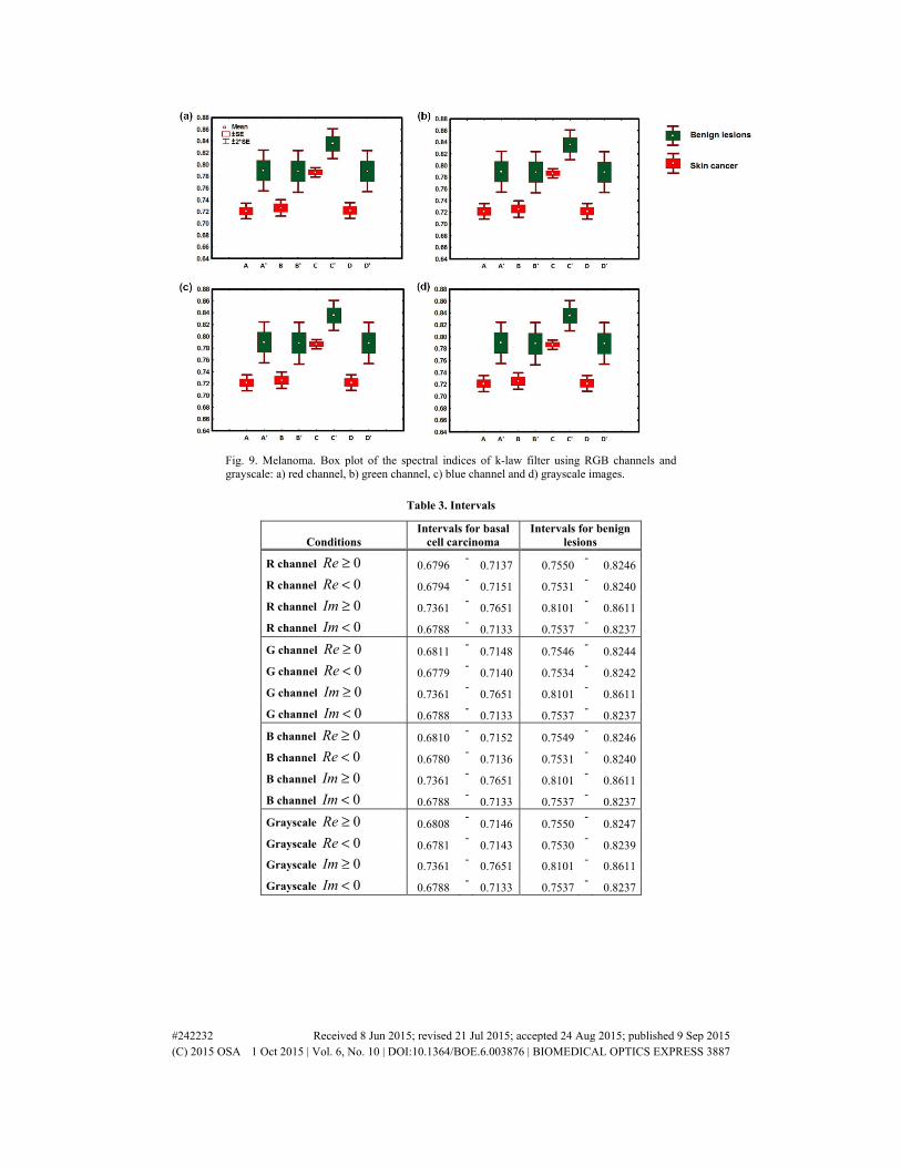
Fig. 9. Melanoma. Box plot of the spectral indices of k-law filter using RGB channels and grayscale: a) red channel, b) green channel, c) blue channel and d) grayscale images.

Table 3. Intervals

Conditions Intervals for basal

cell carcinoma Intervals for benign

lesions


0.7137 0.7550-

0.8246


0.7151 0.7531-

0.8240


0.7651 0.8101-

0.8611


0.7133 0.7537-

0.8237


0.7148 0.7546-

0.8244


0.7140 0.7534-

0.8242


0.7651 0.8101-

0.8611


0.7133 0.7537-

0.8237


0.7152 0.7549-

0.8246


0.7136 0.7531-

0.8240


0.7651 0.8101-

0.8611


0.7133 0.7537-

0.8237


0.7146 0.7550-

0.8247


0.7143 0.7530-

0.8239


0.7651 0.8101-

0.8611


0.7133 0.7537-

0.8237


Table 4. Intervals

Conditions

Intervals for squamous cell

carcinoma

Intervals for benign lesions


0.7143 0.7556 -

0.8239


0.7194 0.7538 -

0.8233


0.7058 0.8106 -

0.8605


0.7162 0.7544 -

0.8230


0.7146 0.7553 -

0.8237


0.7191 0.7541 -

0.8234


0.7058 0.8106 -

0.8605


0.7162 0.7544 -

0.8230


0.7145 0.7556 -

0.8239


0.7193 0.7538 -

0.8233


0.7058 0.8106 -

0.8605


0.7162 0.7544 -

0.8230


0.7149 0.7557 -

0.8240


0.7189 0.7537 -

0.8231


0.7058 0.8106 -

0.8605


0.7162 0.7544 -

0.8230

Table 5. Interval

Conditions Intervals for melanoma

Intervals for benign lesions


0.7340 0.7556 -

0.8239


0.7398 0.7538 -

0.8233


0.7945 0.8106 -

0.8605


0.7349 0.7544 -

0.8230


0.7347 0.7553 -

0.8237


0.7391 0.7541 -

0.8234


0.7945 0.8106 -

0.8605


0.7349 0.7544 -

0.8230


0.7346 0.7556 -

0.8239


0.7393 0.7538 -

0.8233


0.7945 0.8106 -

0.8605


0.7349 0.7544 -

0.8230


0.7345 0.7557 -

0.8240


0.7393 0.7537 -

0.8231


0.7945 0.8106 -

0.8605


0.7349 0.7544 -

0.8230


Table 6 shows a comparison about level of confidence with others works.

Table 6. Comparison with other works

Authors Confidence level

Gola et al. 86%

Rahmana and P. Bhattacharya 72.45%

Cavalcanti and J. Scharcanski 94.54%

Jaleel et al. Good accuracy

Sadegui et al. 94.3%

Barata et al. 82.1%

Betta et al. Good accuracy

Celebi et al. 92.34%

Premaladha and Ravichandran 92%

This work 95.4%

4. Conclusions

This paper presents a new methodology for the diagnosis of skin cancer on images with spots through a spectral analysis using different types of filters such as classic, inverse and k-law nonlinear, making a frequency analysis into the RGB and grayscale channels. The confidence level is of 95.4%.

After testing the filters the results obtained show a no significant difference, this is due to apply the conditions of the spectral density for obtaining the binarized image, therefore any filter on any channel can be used. Images of skin cancer and benign lesion were analyzed. The results show a clear difference between the intervals for the diagnosing of skin cancer and benign lesions. The results show that skin cancer presents a well-defined fringe of spectral indices, so the values obtained inside this fringe will be diagnosed as skin cancer.

It may be helpful for medical doctors who do not have enough experience in dermatology. Finally this system will provide a fast diagnosis for the medical field and it will be a non-invasive tool for the patient, therefore it can help prevent skin cancer

Appendix A

The image is intensity data set in the spatial domain, which is represented by the multispectral

function ( , )cwf x yλ where every pixel coordinate x and y and , ,c R G Bλ = {λ λ λ } where red

(R), green (G) and blue (B) are the channels represented by RGB color model produced by a digital image with a range of [0, 255].

The filter bank is made up of 1 2 3, , ,..., wf f f fλ λ λ λ multispectral functions, w is the image

taken of size N x P pixels where 1,..., N, 1,..., Px y= = .

Each image ( , )cwf x yλ can be separated in their respective RGB channels, thus obtaining

the data for three intensity matrices ( , ), ( , )GRw wf x y f x yλλ and ( , )B

wf x yλ .

Every intensity matrix channel of skin cancer is analyzed by taking an intensity profile

vector set { }q w

λξ where 1,...,q Q= vectors and { } ( , ),cq ww

f x yλλξ ∈ thus{ }q w

λξ can be defined by

{ } ( ), , for ,..., ,2 2

cq w Vtw

Q Qf x Vtλλ ξ = ζ = −

(7)

where ,2t Vt

NV Vt

∈ ζ = + and 1,..., .x P=


Let λΨ

be a vector of mean values of intensity profile vector set, on each channel, where λΨ ∈

, using Eq. (7) these mean values can be calculated as

{ }

ˆ .q wq

w Q

λ

λΣ ξ

Ψ = (8)

30Q = was the value taken in this study for all images. Figure 10 shows the intensity profile

vector set { }q w

λξ with calculated graphics from each skin cancer channel using Eq. (7),

afterwards, using Eq. (8) can be obtained the pattern measurement for every skin cancer

channel , ,GR Bλλ λΨ Ψ Ψ

and GrayΨ

respectively. The x axes represents the distance along

profile

Fig. 10. Intensity profiles, (a) Intensity vector set, (b) mean values of red channel (c) mean values or green channel, (d) mean values of blue channel and (e) mean values of grayscale.

Fig. 11 shows all the intensity profiles, where a small difference between each intensity profile can be observed, however after applying the methodology the results do not present significant difference, thus any color channel or grayscale can be used.


0 100 200 300 4000

50

100

150

200

Frecuencies

Inte

nsity

R channelG channelB channel Grayscale

Fig. 11. Intensity profiles of all channels and grayscale.

Appendix B

Filters allow us to extract the interested information on an image, the methodology presented in this work is based on the classic, inverse and nonlinear k-law.

a) A classic filter [21] is denoted as

( , ) exp ( , ) ,c

j jw w

CF I u v j u vλ= ϕ (9)

where ( , )c

jwI u vλ is the Fourier transformation of the function ( , )c

jwI x yλ and ( ),jw u vϕ is the

phase. b) Inverse filter [22, 23] is defined as

exp ( , )

.( , )

j

c

j

w

w

j u vIF

I u vλ

− ϕ=

(10)

c) A k-law nonlinear filter [24] is expressed as follows

( , ) exp ( , ) ,c

j j

k

w wk lawF I u v j u vλ− = ϕ (11)

Where ( , )c

jwI u vλ is the modulus of the Fourier transform and u, v are variables obtained in the

frequency domain, k is the level of nonlinearity that takes values 0 1k< < , ( ),jw u vϕ is the

phase of the Fourier transform. The nonlinearity factor 0.1k = was used.

Then each filter was applied over the function ( , )c

jwI x yλ to obtain the function for each

filter respectively.

Acknowledgments

This document is based on work partially supported by CONACYT under grant No. 169274 and partially supported by Centro de Investigación Científica y de Educación Superior de Ensenada (CICESE). Esperanza Guerra-Rosas is a student in the PhD Departamento de Investigación en Física offered by Universidad de Sonora and supported by CONACyT’s scholarship.


Documents

Methodology for diagnosing of skin cancer on images of ...usuario.cicese.mx/~josue/pdf/biomedical_optics_express_2015.pdf · Methodology for diagnosing of skin cancer on images of