Embed Size (px)
Citation preview
The Islamic University of Gaza غـــزة - ـامـعـة االسالميةــالج Deanery of Graduate Studies اـــــــات الـعـلـيـــــادة الدراسـعــم Faculty of Engineering ةــــــــــــــــــــندســـهـــــة الـــــــليــــــك
Electrical Engineering Department الكـهربائيـــة ةـــالـهـــندسقسم
Modeling and Control of 5DOF Robot Arm Using Supervisory Control
Ahmed Zakari Alassar
Advisors Dr. Hatem Elaydi
Dr. Iyad Abuhadrous
A Thesis Submitted in Partial Fulfillment of the Requirements for the Degree of Master of Science in
Electrical Engineering
March 2010 1431ربيع أول

iii
ABSTRACT
Modeling and control of 5 degree of freedom (DOF) robot arm is the subject of this thesis. The modeling problem is necessary before applying control techniques to guarantee the execution of any task according to a desired input with minimum error. Deriving both forward and inverse kinematics is an important step in robot modeling based on Denavit Hartenberg (DH) representation.
The main objective of this thesis is to control a robot arm using three controllers to acquire the desired position. Proportional integral derivative (PID) controller is used as a reference benchmark to compare its results with fuzzy logic controller (FLC) and fuzzy supervisory controller (FSC) results. FLC is applied as a second controller because of the nonlinearity in the robot manipulators. We compare the result of the PID controller and FLC results in terms of time response specifications. FSC is a hybrid between the previous two controllers. The FSC is used for tuning PID gains since PID alone performs not satisfactory in nonlinear systems. Hence, comparison of tuning of PID parameters is utilized using classical method and FSC method. Based on simulation results, FLC gives better results than classical PID controller in terms of time response and FSC is better than classical methods such as Ziegler-Nichols (ZN) in tuning PID parameters in terms of time response.

iv
ملخص
مفاصل روبوت من ذوي الخمسة التحكم المراقب لجهاز
ومنذجة الروبوت ضرورية قبل تطبيق . من ذوي اخلمسة مفاصل عىن هذه الرسالة مبشاكل النمذجة والتحكم لذراع آيلت وعند منذجة الروبوت فان . انظمة التحكم وذلك لضمان تنفيذ املهمة املطلوبة وفقا للمدخالت بأقل نسبة خطأ ممكنة
Denavit( احلركة األمامية واحلركة اخللفية حملاور الروبوت هو خطوة اساسية استنادا اىل طريقة اشتقاق كل من
Hartenberg(.
إن اهلدف الرئيس هلذه الرسالة هو التحكم بذراع الربوت باستخدام ثالثة متحكمات للوصول اىل اهلدف كأساس مرجعي ملقارنة نتائجه بنتائج املتحكم ) PID(حيث مت استخدام املتحكم التناسيب التكاملي التفاضلي املطلوب،
كمتحكم ثان نظرا لعدم FLCوقد مت تطبيق املتحكم . (FSC)واملتحكم اإلشرايف الغامض (FLC)املنطقي الغامض لقد مت . بداللة مقياس استجابة الزمن PID مقارنة نتائج هذا املتحكم بنتائج املتحكم ذراع الروبوت، ومن مث متت خطية
بواسطة PIDجيمع بني كال املتحكمني السابقني، ويهدف اىل ضبط معامالت املتحكم FSCتصميم متحكم ثالث وبالتايل سوف نقوم مبقارنة . يف حالة األنظمة الغري خطية يعطي نتائج غري جيدة PIDحيث إن املتحكم FLC املتحكم
بالنتائج اليت مت احلصول عليها باستخدام اساليب الضبط FSCالنتائج اليت مت احلصول عليها باستخدام املتحكم يعطي نتائج FSCو FLCكل من املتحكمني واستنادا اىل نتائج احملاكاة، فان هذه الرسالة تبني أن استخدام . التقليدية
.PIDجيدة مقارنة بالنتائج اليت مت احلصول عليها باستخدام املتحكم

v
Dedicated to
My Father Dr. Zakari Ahmed Alassar
vi
ACKNOWLEDGEMENT
I thank Allah, the lord of the worlds, for His mercy and limitless help and guidance. My peace and blessings be upon Mohammed the last of the messengers.
I would like to express my deep appreciation to my thesis advisor Dr. Hatem Elaydi for providing his advice and encouragement. Also, I am heavily indebted to my supervisor Dr. Iyad Abu Hadrous for his excellent guidance, the warm discussion and regular meeting I had with him during research. I would like to thank the other committee members Dr. Assad Abu-Jasser and Dr. Basel Hamed for providing their valuable suggestions. In addition, my thanks go to my friends and colleagues for their advices and supports.
There are no words that describe how grateful I am to my parents Dr. Zakari Alassar and my mother for raising me and for their support and encouragement through years. My deepest thanks go to my brothers Mohammed and Yahiya and my sister. Lastly, I am grateful to my wife and my kids Yusuf and Zakaria for their patience and understanding during my busy schedule.
vii
TABLE OF CONTENTS
ABSTRACT ................................................................................................................................................. III
IV ............................................................................................................................................................ ملخص
ACKNOWLEDGEMENT .......................................................................................................................... VI
TABLE OF CONTENTS ......................................................................................................................... VII
LIST OF FIGURES .................................................................................................................................... IX
LIST OF TABLES ...................................................................................................................................... XI
NOMENCLATURE .................................................................................................................................. XII
ABBREVIATIONS .................................................................................................................................... XV
CHAPTER 1 INTRODUCTION ........................................................................................................... 1
1.1. MOTIVATION ................................................................................................................................ 1 1.2. BACKGROUND .............................................................................................................................. 2
1.2.1. Linear and Nonlinear Control .................................................................................................... 5 1.2.2. Independent Joint Control .......................................................................................................... 5 1.2.3. Control Techniques ..................................................................................................................... 6
1.3. LITERATURE REVIEW ................................................................................................................... 7 1.4. PROBLEM STATEMENT ................................................................................................................. 9 1.5. THESIS OBJECTIVES AND METHODOLOGIES ................................................................................ 9 1.6. THESIS CONTRIBUTION .............................................................................................................. 10 1.7. THESIS STRUCTURE .................................................................................................................... 10
CHAPTER 2 KINEMATICS AND MATHEMATICAL MODELING ......................................... 12
2.1. INTRODUCTION ........................................................................................................................... 12 2.2. KINEMATIC ANALYSIS ............................................................................................................... 14
2.2.1 Forward Kinematic .................................................................................................................... 14 2.2.2. Inverse Kinematic ...................................................................................................................... 17
2.3. DC MOTOR MODELING .............................................................................................................. 17 2.4. SUMMARY .................................................................................................................................. 22
CHAPTER 3 PID CONTROLLER DESIGN .................................................................................... 23
3.1. INTRODUCTION ........................................................................................................................... 23 3.2. PID STRUCTURE ......................................................................................................................... 23
3.2.1. Controller Design Methods ....................................................................................................... 25 3.2.2. PID Characteristic Parameters ................................................................................................ 28
3.3. FEEDFORWARD DISTURBANCE REJECTION ................................................................................ 31 3.4. IMPLEMENTATION OF N INDEPENDENT JOINT CONTROL ........................................................... 33 3.5. SUMMARY .................................................................................................................................. 36
CHAPTER 4 FUZZY LOGIC CONTOLLER ................................................................................... 37
4.1. INTRODUCTION ........................................................................................................................... 37 4.2. PRELIMINARIES ON FLC ............................................................................................................. 38
4.2.1. Fuzzy Sets, Fuzzy Subset, and Null Fuzzy Set .......................................................................... 38 4.2.2. Membership Function Features ................................................................................................ 39 4.2.3. Linguistic Variable .................................................................................................................... 40 4.2.4. Linguistic Value......................................................................................................................... 40 4.2.5. Fuzzy Conditional Statement .................................................................................................... 41 4.2.6. Operations on Fuzzy Sets .......................................................................................................... 41
4.3. FLC STRUCTURE ........................................................................................................................ 43 4.3.1. Fuzzification .............................................................................................................................. 44 4.3.2. Knowledge Base ........................................................................................................................ 46 4.3.3. Inference Mechanism ................................................................................................................ 48 4.3.4 Defuzzification ............................................................................................................................ 49
viii
4.4. FUZZY CONTROL ........................................................................................................................ 50 4.5. SUMMARY .................................................................................................................................. 53
CHAPTER 5 FUZZY SUPERVISORY CONTROLLER ................................................................ 55
5.1. INTRODUCTION ........................................................................................................................... 55 5.2. FUZZY SUPERVISORY CONTROLLER STRUCTURE ...................................................................... 55 5.3. FUZZY CONTROLLER DESIGN ..................................................................................................... 59 5.4. RULE BASE DERIVATION............................................................................................................ 61 5.5. SUMMARY .................................................................................................................................. 64
CHAPTER 6 RESULTS ....................................................................................................................... 65
6.1. INTRODUCTION ........................................................................................................................... 65 6.2. LYNX6 AS CASE STUDY ............................................................................................................. 65 6.3. SUMMARY .................................................................................................................................. 78
CHAPTER 7 CONCLUSION AND FUTURE WORK .................................................................... 79
7.1. CONCLUSION .............................................................................................................................. 79 7.2. FUTURE WORK ............................................................................................................................ 80
REFERENCES ........................................................................................................................................... 81
PUBLICATION ......................................................................................................................................... 85
APPENDIX A: FORWARD AND INVERSE KINEMATICS ANALYSIS ........................................ 86
APPENDIX B: ROOT LOCUS ANALYSES METHOD ....................................................................... 94
APPENDIX C: FUZZY MEMBERSHIP FUNCTION AND DEFUZZIFICATION ......................... 96
APPENDIX D: MATLAB, SIMULINK AND GUI .............................................................................. 102
ix
LIST OF FIGURES
Figure 1.1: Manipulator with Revolute and Prismatic Joints [1] ................................ 3 Figure 1.2: Block diagram of a closed-loop control system ........................................ 4 Figure 1.3: The basic structure of (SISO) system ....................................................... 5 Figure 2.1: Robot manipulator with PPP joints ......................................................... 12 Figure 2.2: Schematic of DC motor system .............................................................. 18 Figure 2.3: Block diagram for DC motor system. ..................................................... 19 Figure 2.4: DC motor subsystem using SIMULINK ................................................ 19 Figure 2.5: DC motor open loop step response without load .................................... 21 Figure 2.6: DC motor model simulation with load disturbance ................................ 21 Figure 3.1: PID controller structure .......................................................................... 24 Figure 3.2: Step response of P, PD, and PID controllers .......................................... 25 Figure 3.3: Plant step response in Z-N method ......................................................... 27 Figure 3.4: SIMULINK model of PID controller ...................................................... 28 Figure 3.5: Unit step response curve showing , , .r st t O S and SSE ............................. 29
Figure 3.6: Transient response to step reference input .............................................. 30 Figure 3.7: Transient response to step disturbance input .......................................... 30 Figure 3.8: Servomotor model ................................................................................... 31 Figure 3.9: Closed loop system with disturbance input ............................................ 32 Figure 3.10: Feedforward compensation ..................................................................... 32 Figure 3.11: PID controller with feedforward compensator ....................................... 33 Figure 3.12: IJC for 5DOF using SIMULINK ............................................................ 34 Figure 3.13: Input angles with saturation boundaries ................................................. 34 Figure 3.14: Input menu .............................................................................................. 35 Figure 3.15: Subsystem 3 under the mask ................................................................... 35 Figure 3.16: One joint variable .................................................................................... 36 Figure 4.1: (a) Triangular MFs (b) Singleton MFs ................................................... 39 Figure 4.2: Example of fuzzy linguistic variable ...................................................... 40 Figure 4.3: Union of fuzzy set A and B ..................................................................... 41 Figure 4.4: Intersection of fuzzy set A and B ............................................................ 42 Figure 4.5: Complement of fuzzy set A ..................................................................... 42 Figure 4.6: Fuzzy control system structure ............................................................... 44 Figure 4.7: Membership functions shapes ................................................................. 45 Figure 4.8: Membership function for inputs e and e ............................................... 45 Figure 4.9: Membership function for output u .......................................................... 46 Figure 4.10: Inference process using Mamdani and Larson methods ......................... 49 Figure 4.11: Defuzzification methods ......................................................................... 50 Figure 4.12: Three input fuzzy PID (Type I) .............................................................. 51 Figure 4.13: Three input fuzzy PID (Type II) ............................................................. 51 Figure 4.14: Two input fuzzy PID (Type I) ................................................................ 52 Figure 4.15: Two input fuzzy PID (Type II) ............................................................... 52 Figure 4.16: Output of fuzzy PD and fuzzy PI for r = 60. .......................................... 53 Figure 4.17: a) fuzzy PD + fuzzy I, b) fuzzy PD +I .................................................... 53 Figure 5.1: Fuzzy supervisory control structure ........................................................ 57 Figure 5.2: Fuzzy inference block ............................................................................. 58 Figure 5.3: Input variables of fuzzy controller .......................................................... 58 Figure 5.4: PID parameters membership functions ................................................... 59 Figure 5.5: Fuzzy supervisory: first method ............................................................. 60
x
Figure 5.6: Fuzzy supervisory: second method ......................................................... 60 Figure 5.7: Waveform showing (a) output, (b) error ................................................. 62 Figure 5.8: Step response .......................................................................................... 62 Figure 6.1: Lynx6 robot arm ..................................................................................... 65 Figure 6.2: Frame assignment for the Lynx 6 robot arm. .......................................... 66 Figure 6.3: Lynx6 home position .............................................................................. 67 Figure 6.4: Lynx6 desired position ............................................................................ 67 Figure 6.5: PID control step response for 1 2, ......................................................... 68
Figure 6.6: PID control step response for 3 ............................................................. 68
Figure 6.7: PID control step response for 4 5and .................................................. 69
Figure 6.8: Output with disturbance for 1 2, ........................................................... 70
Figure 6.9: Output with disturbance for 5 ................................................................ 71
Figure 6.10: Output with disturbance rejection for 1 ................................................ 71
Figure 6.11: Output with disturbance rejection for 2 and 5 ..................................... 72
Figure 6.12: FLC step response for 1 and 2 ............................................................... 73
Figure 6.13: FLC step response for 3 ........................................................................ 74
Figure 6.14: FLC step response for 4 ......................................................................... 74
Figure 6.15: FLC step response for 5 ......................................................................... 75
Figure 6.16: Output response using classical tuning methods .................................... 76 Figure 6.17: Output response using fuzzy supervisory control ................................... 76 Figure 6.18: PID parameters variations ....................................................................... 77 Figure A.1: Obtain DH parameters using MATHEMATICA .................................... 86 Figure A.2: A matrices for Lynx6 robot arm .............................................................. 87 Figure C.1: Centroid defuzzification method ............................................................. 97 Figure C.2: Bisector defuzzification method .............................................................. 97 Figure C.3: Mean of Max defuzzification method ..................................................... 98 Figure C.4: Largest of Maximum defuzzification method ......................................... 98 Figure C.5: Smallest of Maximum defuzzification method ....................................... 99 Figure D.1: Independent joint control of five DOF robot arm ................................. 102 Figure D.2: Fuzzy PID controller ............................................................................. 103 Figure D.3: Fuzzy supervisory controller ................................................................. 103 Figure D.4: PID controller ........................................................................................ 104 Figure D.5: Output response using FSC with PID parameter variations……….…..104
xi
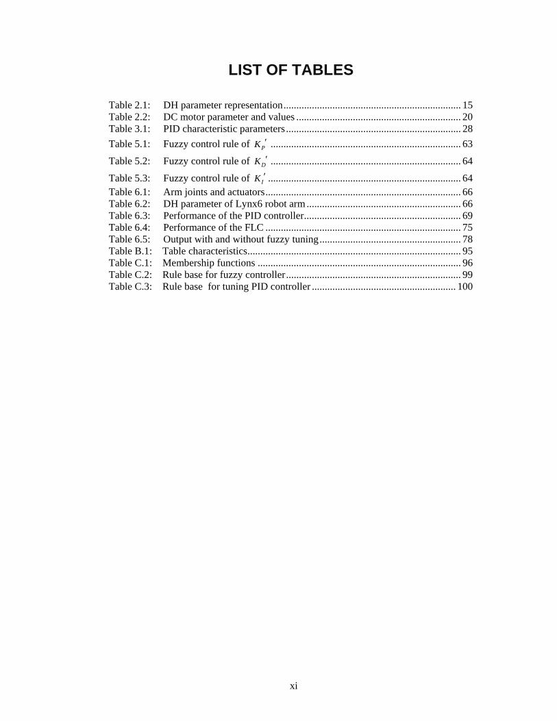
LIST OF TABLES
Table 2.1: DH parameter representation ..................................................................... 15 Table 2.2: DC motor parameter and values ................................................................ 20 Table 3.1: PID characteristic parameters .................................................................... 28
Table 5.1: Fuzzy control rule of PK .......................................................................... 63
Table 5.2: Fuzzy control rule of DK .......................................................................... 64
Table 5.3: Fuzzy control rule of IK ........................................................................... 64 Table 6.1: Arm joints and actuators ............................................................................ 66 Table 6.2: DH parameter of Lynx6 robot arm ............................................................ 66 Table 6.3: Performance of the PID controller ............................................................. 69 Table 6.4: Performance of the FLC ............................................................................ 75 Table 6.5: Output with and without fuzzy tuning ....................................................... 78 Table B.1: Table characteristics ................................................................................... 95 Table C.1: Membership functions ............................................................................... 96 Table C.2: Rule base for fuzzy controller .................................................................... 99 Table C.3: Rule base for tuning PID controller ........................................................ 100
xii
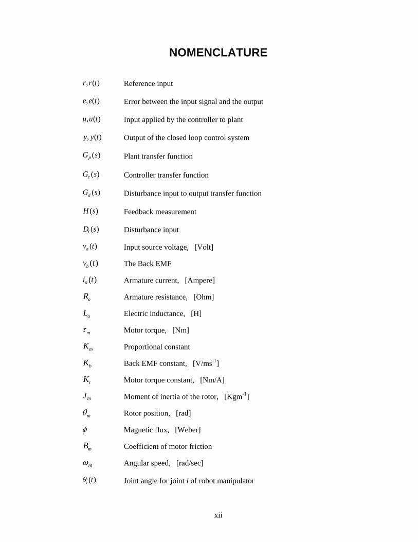
NOMENCLATURE
, ( )r r t Reference input
, ( )e e t Error between the input signal and the output
, ( )u u t Input applied by the controller to plant
, ( )y y t Output of the closed loop control system
( )pG s Plant transfer function
( )cG s Controller transfer function
( )dG s Disturbance input to output transfer function
( )H s Feedback measurement
( )tD s Disturbance input
( )av t Input source voltage, [Volt]
( )bv t The Back EMF
( )ai t Armature current, [Ampere]
aR Armature resistance, [Ohm]
aL Electric inductance, [H]
m Motor torque, [Nm]
mK Proportional constant
bK Back EMF constant, [V/ms-1]
tK Motor torque constant, [Nm/A]
mJ Moment of inertia of the rotor, [Kgm-1]
m Rotor position, [rad]
Magnetic flux, [Weber]
mB Coefficient of motor friction
m Angular speed, [rad/sec]
( )i t Joint angle for joint i of robot manipulator
xiii
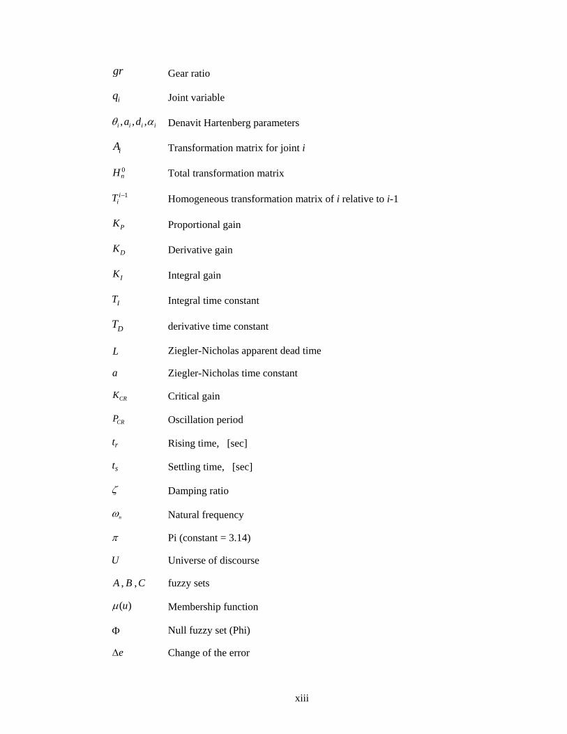
gr Gear ratio
iq Joint variable
, , ,i i i ia d Denavit Hartenberg parameters
iA Transformation matrix for joint i
0nH Total transformation matrix
1iiT Homogeneous transformation matrix of i relative to i-1
PK Proportional gain
DK Derivative gain
IK Integral gain
IT Integral time constant
DT derivative time constant
L Ziegler-Nicholas apparent dead time
a Ziegler-Nicholas time constant
CRK Critical gain
CRP Oscillation period
rt Rising time, [sec]
st Settling time, [sec]
Damping ratio
n Natural frequency
Pi (constant = 3.14)
U Universe of discourse
A , B ,C fuzzy sets
( )u Membership function
Null fuzzy set (Phi)
e Change of the error
xiv
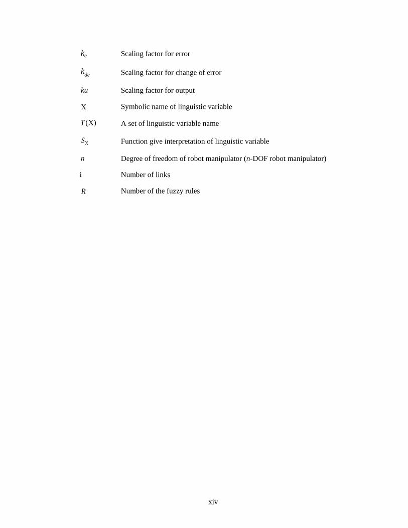
ek Scaling factor for error
dek Scaling factor for change of error
ku Scaling factor for output
Symbolic name of linguistic variable
( )T A set of linguistic variable name
S Function give interpretation of linguistic variable
n Degree of freedom of robot manipulator (n-DOF robot manipulator)
i Number of links
R Number of the fuzzy rules
xv
ABBREVIATIONS
BOA Bisector of Area
COA Centroid of Area
CL Closed Loop
DOF Degree of Freedom
DH Denavit Hartenberg
DC Direct Current
DFC Direct Fuzzy Controller
EMF Electromagnetic Force
FITA First Inference Then Aggregation
FK Forward Kinematic
FGS Fuzzy Gain Scheduling
FLC Fuzzy Logic Controller
FPD Fuzzy Proportional Derivative Controller
FPI Fuzzy Proportional Integral Controller
FSC Fuzzy Supervisory Control
GMP General Modus Ponens
GMT General Modus Tollens
GUI Graphical User Interface
IJC Independent Joint Control
IFC Indirect Fuzzy Controller
IK Inverse Kinematic
LOM Largest of Maximum
Max Maximum
MM Maximum Method
MOM Mean of Maximum
xvi
MF Membership Function
Min Minimum
MIMO Multi Input Multi Output
MISO Multi Input Single Output
NN Neural Network
OL Open Loop
P Prismatic
PID Proportional Integrated Derivative
R Revolute
SIMO Single Input Multi Output
SISO Single Input Single Output
SOM Smallest of Maximum
TS Takagi Sugeno
TF Transfer Function
Z-N Ziegler-Nicholas
Modeling and Control of 5DOF Robot Arm Using Supervisory Control
1
CHAPTER 1 INTRODUCTION
1.1. Motivation
In recent years, industrial and commercial systems with high efficiency and great performance have taken advantages of robot technology. Large number of control researches and numerous control applications were presented during the last years, concentrated on control of robotic systems. Robot manipulator field is one of the interested fields in industrial, educational and medical applications. It works in unpredictable, hazard and inhospitable circumstances which human cannot reach. For example, working in chemical or nuclear reactors is very dangerous, while when a robot instead human it involves no risk to human life. Therefore, modeling and analysis of the robot manipulators and applying control techniques are very important before using them in these circumstances to work with high accuracy.
In Gaza strip, many industrial applications can utilize robot technology and develop robot manipulators. It is an attractive field to be applied and developed for industrial applications. This thesis is meant to be suitable for these applications. On the other side, some universities and colleges offers, some courses related to robotics. These courses mainly focus on the theoretical concepts without giving much attention for controlling different robot manipulators in the practical side. This thesis may be considered as a valuable educational tool in their laboratories.
The essential problem is to study the robot manipulator problem from two sides: the first one is the mathematical modeling of the manipulator and the actuators, which includes an analysis for the forward kinematic, the inverse kinematic and modeling the direct current (DC) motor because it is an important issue in a robot manipulator. The second problem is the control of the robot manipulator.
The main objective of this thesis is concerned with designing a controller for the motion of the robot manipulator to meet the requirement of the desired trajectory input with suitable error and disturbance values. The motivation of control technique designs the usage of the high precision performance of the robot manipulators in complicated and hazardous environments.
Various controllers have been designed and applied in the robot manipulator. The first question that may arise is the different types of these controllers and the difference between these controllers in terms of best performance will be shown.
Proportional Integral Derivative (PID) controller may be the most widely used controller in the industrial and commercial applications for the early decades, due to its simplicity of designing and implementation, so the first attempt is to apply PID control; however, PID does not give optimal performance due to the nonlinear elements. Robot manipulators are classified as nonlinear systems, so classical controllers are not sufficient to give the best results. Fuzzy logic controller (FLC) was found to be an efficient tool to control nonlinear systems. Designing and testing FLC will be shown as a second option.
In recent years, hybrid between fuzzy and classical controllers has combined to design a controller such as fuzzy plus PID and fuzzy logic supervisory (FLS) creates more appropriate solution to control robot manipulator. Through the thesis, FLC is considered as an important controller for on-line tuning of PID parameters. FLC may design to monitor and enhance the PID parameters online.
Chapter 1 Introduction
2
The robot movements' analysis is important before the implementation of the actual system in order to prevent possible environmental hazards. Therefore, computer simulations are important to perform any controller, where developing distinct mathematical model for any robot manipulator is an important issue to perform the simulations.
1.2. Background
According to the RIA1, a robot is a “reprogrammable multifunctional manipulator designed to move material, parts, tools, or specialized devices through variable programmed motions for the performance of a variety of tasks” [1]. Through this thesis, the term “robot manipulator” is used.
Robot manipulator is one of the motivating disciplines in industrial and educational applications, and an essential branch to control sciences because of its intelligent aspects, nonlinear characteristics, and its real time implementation. It was developed to enhance human’s work such as in the manufacturing or manipulation of heavy materials, and unpredictable environments. Whatever the kind of task robot manipulator may be provided with, robot performance measures the high quality and large quantity of work that it can do in the desired time and place. Robot manipulator has immeasurable tasks, so it is designed to be flexible in general motions to move from one position to another with smooth movement to avoid sharp jolt in the robot arm. These jolts may damage the arm.
There are three main subsystems in robot manipulators: mechanical system, electrical system, and control system [2]. Mechanical system comprises of all movable parts. It consists of a group of links (rigid bodies) connected together by joints which allow the motion for the desired link. The mechanical system is used to move the end effector (the top link) to xyz position with respect to the base. This movement depends on the electrical system (e.g. motors, power amplifiers, and other electronic circuits) and it is done by some rotations and translations to the other links. Due to the varity of tasks and duties in robot manipulators, its construction is divided into two main classes: serial manipulator and parallel manipulators [2].
Serial manipulators consist of some links connected in series, which form an open loop chain. At the end of the chain, the end effector is connected to the base by single kinematic chain. On the other side, the parallel manipulators form a closed loop chain finished by the end effector and is connected to the base by two, or more kinematic chains (e.g. arm, or legs). The only drawback of the parallel manipulator over the serial manipulator is that the parallel robots manipulators suffer from limited workspace as compared with serial robot manipulators.
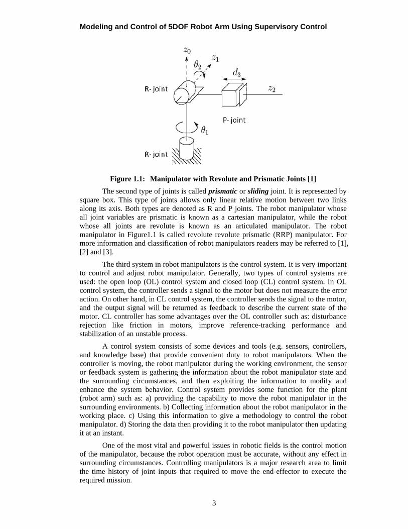
Figure 1.1 shows a schematic diagram of a robot manipulator. It consists of three joints and each one of these joints will have a motor to actuate the desired link. There are two widespread types of joints on this manipulator. The first type is represented by a cylinder, and it allows only relative rotation between two links. This type of joint is called revolute or rotary joint (e.g. human joints), and it is the most common joint type in robots.
1 RIA: Robot Institute of America
Modeling and Control of 5DOF Robot Arm Using Supervisory Control
3
Figure 1.1: Manipulator with Revolute and Prismatic Joints [1]
The second type of joints is called prismatic or sliding joint. It is represented by square box. This type of joints allows only linear relative motion between two links along its axis. Both types are denoted as R and P joints. The robot manipulator whose all joint variables are prismatic is known as a cartesian manipulator, while the robot whose all joints are revolute is known as an articulated manipulator. The robot manipulator in Figure1.1 is called revolute revolute prismatic (RRP) manipulator. For more information and classification of robot manipulators readers may be referred to [1], [2] and [3].
The third system in robot manipulators is the control system. It is very important to control and adjust robot manipulator. Generally, two types of control systems are used: the open loop (OL) control system and closed loop (CL) control system. In OL control system, the controller sends a signal to the motor but does not measure the error action. On other hand, in CL control system, the controller sends the signal to the motor, and the output signal will be returned as feedback to describe the current state of the motor. CL controller has some advantages over the OL controller such as: disturbance rejection like friction in motors, improve reference-tracking performance and stabilization of an unstable process.
A control system consists of some devices and tools (e.g. sensors, controllers, and knowledge base) that provide convenient duty to robot manipulators. When the controller is moving, the robot manipulator during the working environment, the sensor or feedback system is gathering the information about the robot manipulator state and the surrounding circumstances, and then exploiting the information to modify and enhance the system behavior. Control system provides some function for the plant (robot arm) such as: a) providing the capability to move the robot manipulator in the surrounding environments. b) Collecting information about the robot manipulator in the working place. c) Using this information to give a methodology to control the robot manipulator. d) Storing the data then providing it to the robot manipulator then updating it at an instant.
One of the most vital and powerful issues in robotic fields is the control motion of the manipulator, because the robot operation must be accurate, without any effect in surrounding circumstances. Controlling manipulators is a major research area to limit the time history of joint inputs that required to move the end-effector to execute the required mission.
Chapter 1 Introduction
4
Generally, a controller is used to modify the behavior of the physical system according to the input value through computations and actuations. Over the early decade, numerous control techniques and methodologies have been proposed to control the motion of the robot manipulators such as point-to-point, sequencing “continuous path”, speed and incremental motions. As an example, the first control method capable for stopping at several different programmed positions, it can be used to pick and place operations. The required control method is chosen depending on the type of the robot manipulator and its possible applications. Varity of robot manipulators and their architectures influence the control methodology, for example, to control the robot manipulator movement between two points x and y (point to point) needs a different controller than the continuous path tracking. On the other hand, the mechanical design of the manipulator affects the controller type; for example, if there are two robots: one has RRR or (3R) joints as PUMA 560 and the other has PPP or (3P) joints as cartesian robot, then the control problems encountered with the RRR different from those encountered the PPP.
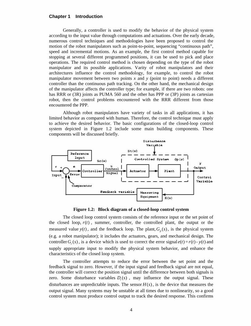
Although robot manipulators have variety of tasks in all applications, it has limited behavior as compared with human. Therefore, the control technique must apply to achieve the desired behavior. The basic configurations of the closed-loop control system depicted in Figure 1.2 include some main building components. These components will be discussed briefly.
Figure 1.2: Block diagram of a closed-loop control system
The closed loop control system consists of the reference input or the set point of the closed loop, ( )r t , summer, controller, the controlled plant, the output or the
measured value ( )y t , and the feedback loop. The plant, ( )pG s , is the physical system
(e.g. a robot manipulator); it includes the actuators, gears, and mechanical design. The controller ( )cG s , is a device which is used to correct the error signal ( )e t = ( )r t - ( )y t and
supply appropriate input to modify the physical system behavior, and enhance the characteristics of the closed loop system.
The controller attempts to reduce the error between the set point and the feedback signal to zero. However, if the input signal and feedback signal are not equal, the controller will correct the position signal until the difference between both signals is zero. Some disturbance variables ( )tD s , may influence the output signal. These
disturbances are unpredictable inputs. The sensor ( )H s , is the device that measures the output signal. Many systems may be unstable at all times due to nonlinearity, so a good control system must produce control output to track the desired response. This confirms
Modeling and Control of 5DOF Robot Arm Using Supervisory Control
5
that the important issue in designing a control system is to ensure that the dynamic response of the closed loop systems is stable.
1.2.1. Linear and Nonlinear Control
There are two methods used in control theory to control systems, linear method and nonlinear method. Using linear control is applicable only when the controlled system can be modeled mathematically [3]. The facts that the majority of physical systems have nonlinear characteristics; hence, linear controllers fail to meet the requirements due to system nonlinearities. The variations and the nonlinear parameters such as gear backlash, load variations and other parameters have unpredictable effects on the controlled systems (e.g. robot manipulator) diminish the performance. Therefore, the robot manipulator may be considered as a linear model when it works on small space, or it has a large gear ratio between the joints and their links. Nonlinear methods considered as general case when compared to linear methods because it can be applied successfully on the linear methods, but linear method is not sufficient to solve and control nonlinear problems. Common methodologies are used to solve the nonlinearities in control systems such as sliding mode control, and state feedback control are discussed in [4].
1.2.2. Independent Joint Control
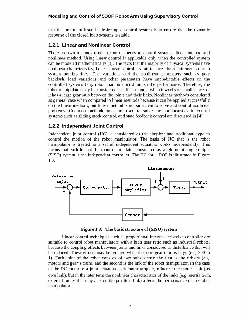
Independent joint control (IJC) is considered as the simplest and traditional type to control the motion of the robot manipulator. The basis of IJC that is the robot manipulator is treated as a set of independent actuators works independently. This means that each link of the robot manipulator considered as single input single output (SISO) system it has independent controller. The IJC for 1 DOF is illustrated in Figure 1.3.
Figure 1.3: The basic structure of (SISO) system
Linear control techniques such as proportional integral derivative controller are suitable to control robot manipulators with a high gear ratio such as industrial robots, because the coupling effects between joints and links considered as disturbance that will be reduced. These effects may be ignored when the joint gear ratio is large (e.g. 200 to 1). Each joint of the robot consists of two subsystems: the first is the drivers (e.g. motors and gear’s train), and the second is the link of the robot manipulator. In the case of the DC motor as a joint actuators each motor torque t influence the motor shaft (its
own link), but in the later term the nonlinear characteristics of the links (e.g. inertia term, external forces that may acts on the practical link) affects the performance of the robot manipulator.
Chapter 1 Introduction
6
1.2.3. Control Techniques
Due to uncertainty and instability effects, unknown or unpredictable inputs that manipulate the plant output to the incorrect target. These inputs are called disturbance or noise, so analyzing and designing the mathematical model of the system includes the controller and plants to get the desired behavior is required. Many control techniques have been proposed to control robot manipulator ranging in complexity from linear to the advanced control system, which compute the robot dynamic and save it from damage in real environments. Three different control schemes namely PID controller, FLC, and the fuzzy supervisory controller (FSC) will be implemented through this thesis. The performance of these controllers will be based on the high precision in reducing the overshoot, minimizing steady state error, damping unwanted vibration of robot manipulator, and handling the unpredictable disturbances.
PID controller is one of the earliest controllers in the industrial robot manipulators, so the first attempt to control the plant is use the PID controller. PID controller is still considered the most widely used in industry [5] and [6]. The popularity of using the PID or the PID-types controllers is that they have a simple structure, and they give satisfactory results when the requirements are reasonable and the process parameters variations are limited. In addition, the majority of applications are familiar with the PID controller based on the knowledge of the system characteristics. Several techniques used for tuning PID parameters that have been developed over the past decade such as Ziegler-Nichols (Z-N) tuning methods [7]. One of the drawbacks for using the PID control techniques is that, they are not sufficient to obtain the desired tracking control performance because of the nonlinearity of the robot manipulator. Hence, a lot of time is required to tune the PID parameters. On the other hand, other techniques are used to overcome the previous problem, such as fuzzy controller that emulates human operation.
FLC is an emerging technique in control systems. It is considered as intelligent controller. Many studies show that the fuzzy controller (FC) performs superior to conventional controller algorithms will be discussed in the next section. Zadeh [8] did the main idea of FLC and fuzzy set theory. Mamdani and his colleagues [9] have done a pioneering research work on FLC in the mid-’70 for engine steam boiler. The benefit of FLC is obvious when the controlled process is too complicated to be analyzed using PID controller or when the information about the controlled system does not exist.
FLC is classified into two categories: the first, involves the fuzzy logic system based on a rule based on expert system, to determine the control action. The second used FL to provide online adjustment for the parameters of the conventional controller such as the PID control [10]. This method attempts to combine the merits of FL with those control techniques to expand the capability of linear control technique to handle the nonlinearity in the physical system. Fuzzy supervisory is used to reduce the amount of tuning the PID controller with a fuzzy system [11]. It is considered as an attractive method to solve the nonlinear control problems, one of the advantages of fuzzy supervisory that the control parameters changed rapidly with respect to the variation of the system response. The fuzzy supervisor operates in a manner similar to that of the FLC and adds a higher level of control to the existing system. Fuzzy supervisory is hybrid between the PID controller and FLC that designed to overcome the problem of tuning PID in nonlinear systems using FLC as an adaptive controller [12]. The basic structure of FSC resembles the structure of PID controller, but the controlled parameter of PID controller depends on the output of the fuzzy controller.
Modeling and Control of 5DOF Robot Arm Using Supervisory Control
7
1.3. Literature Review
Generally, robotic system is designed and developed to assist or replace a human in doing and accomplishing tasks that are boring, complex, too dangerous, and impossible for human. As an advanced investigation in this emerging field, a vast number of researches have been proposed over the last two decades for robot manipulator fields, some of these literatures discussed the kinematics analysis of industrial and educational robots such as PUMA 560, SCARA, and SG5-UT robot manipulators [11], [13] [14] and [15]. Other papers discussed control technique problems, such as PID, FLC and other techniques [16], [17], [18], [19] and [20]. A good review of some literatures is listed next:
Kinematics of robot arm was mathematically modeled using a Denavit Hartenberg (DH) method [1], [2] and [3]. Forward and Inverse equation analysis, were generated and implemented using a simulation program [21] and [22]. In [14] Annand derived the kinematics analysis of PUMA 560, and calculated the equation of motion of the robot by deriving the so-called Euler-Lagrange equations. In [23] achieving a high level of complexity for robotic system design was straightforward and highly intuitive when using the PTOLEMY II software environment. After deriving the inverse kinematics equations, Antonia used PTOLEMY II to design, and simulate robot arm. The benefit of this software is that designing complicated system requires simple building blocks.
Elgazzar presented in her paper [15] efficient solutions for the kinematics positions, velocities, and accelerations for the 6DOF PUMA 560 robots. The solution method was based on a method that fully exploits the special geometry of the robot in the derivation of the solution. Elgazzar showed that for the accurate control of the arm motions all these solutions were needed, resulting in a substantial saving in computation time, and a critical consideration for real time control.
Position control performed using independent joint control in [1]. This method was using PID controller, and it worked by controlling each joint independently. The coupling effect between the joints and links could be ignored if the gear ratio was large.
The work presented by Delibasi [24] illustrated the position control of DC motor using FLC and PID control algorithms. Both two controllers were designed based on LABVIEW program. After applying controllers, results showed that the desired position was achieved with 0.4% overshoot, and 80msec settling time for fuzzy controller, but when using PID controller with the overshoot is 4%, and the settling time is 120msec. Delibasi featured the influence of FLC upon the performance of robot movement simulation, which was controlled by a digital controller. Khoury [18] presented the design of a fuzzy logic controller of 5DOF robot arm. Through his paper, he introduced two structures of FLC: first three inputs with coupled rule base and the second structure was two inputs with coupled rules. Khoury confirmed the success of the proposed fuzzy controller. In addition, when a fuzzy controller in comparison to other nonlinear controls, it confirmed again the success in tracking control system.
In [25] the performance between proportional derivative fuzzy logic controllers (PDFLC) with 5 membership functions (MF) controller and PDFLC with 7 MFs controller was analyzed in terms of time response specifications and integral square error. Based on the simulation result Samin proved that PDFLC with 5 MFs was better than PDFLC with 7 MFs. For the time response performance, the PDFLC with 5 MFs produced settling time and rise time of 0.247sec and 0.156sec respectively whereas the
Chapter 1 Introduction
8
PDFLC with 7 MFs produced settling time and rise time of 0.298sec and 0.184sec respectively. It showed that the PDFLC with 35 rules and 7 MFs resulted in a slower response as in comparison to PDFLC with 11 rules and 5 MFs.
Wei_Li [26] presented an approach to combining a fuzzy logic controller with PID controller. In his paper, he replaced the proportional term in the conventional controller with fuzzy P controller for implementing fuzzy P+ID controller. The proposed controller (fuzzy P+ID) combined the advantages of the fuzzy controller and conventional controller. Comparison between the existing controller and PID controller Wei_Li shows that the fuzzy P term improved the overshoot and rising time while as the conventional terms; I and D controllers reduced the steady state error and enhanced the system stability. Wei_Li presented two features of his controller: first fuzzy P+ID controller kept the simple structure of PID controller, second the stability condition unchanged if the fuzzy P + ID controller replaced the PID controller.
In [19], the PDFLC fuzzy controller was combined with PID controller to enhance the performance and robustness of the controller. Simulation results showed that the combined structure did a very good controller. The work presented by Yang and Chen in [27] compared two fuzzy controllers: PDFLC and PIFLC. They proved by simulation that the PDFLC better than PIFLC. In PDFLC, response had a larger steady-state error than PIFLC response and the PIFLC response was less damped with an overshoot. Therefore, he combined two controllers to improve the step response.
In [16], two controllers were used for robot movement, with and without FLC. Soh and Alwi proved that the system with FC was found to be more efficient, where it increased the system stability. Mathematical model was developed for 3 DOF robot arm, FLC and neural network (NN) was developed to trace desired trajectory for 3 DOF robot arm. A fuzzy controller was applied to an inverted pendulum and was presented in [28]. Chopra and colleagues proved that increasing the rules beyond that limit was ineffective. Secondly, the rules can be reduced using the fuzzy subtractive clustering (FSC) approach, and it gave similar performance as by the larger rule set. The rules were reduced to 8 from 81, 49 and 25. Simulation and comparison of results had shown effectiveness of a proposed fuzzy controller using FSC approach. MATLAB simulation was presented in [17] proved that the fuzzy PID controller achieved better performance as in comparison to traditional controllers.
Khong [29] was applied FLC to control the position of DC servomotor. He explained that the result of the experiment with fuzzy controller reached the reference position and speed without any overshoot. The results of an experiment showed that the position control of DC servomotor was investigated with optimal performance and the proposed controller achieved and overcame the disadvantage of the conventional PID control sensitivity to inertia variation and sensitivity to variation of the position with the drive system of DC servomotor.
Sreentha and Pradhanb in [30] designed FLC for the position control of a revolute, single flexible link. The FLC was based on 49 IF-THEN rules and used the error in the angular displacement at the joint and its time rate of change as input variables. Both theoretical and experimental results showed that the angular displacement at the base joint was highly oscillatory and suffered from an excessively large settling time.
Surdhar and White [31] focused on the control of a nonlinear two-axis manipulator with a single flexible link. They used a PD controller with the gain of the derivative term being adjusted by a FLC whose measured inputs are the error and error
Modeling and Control of 5DOF Robot Arm Using Supervisory Control
9
change. The results showed that the fuzzy PD controller exhibited shorter settling time, smaller steady state error and handled some nonlinearity than the conventional PD controller. In [32] Nil and Yuzgec proved that the proposed FLC and NN control had reached the desired performance, and NN control traced the desired trajectory closer and smoother than the FLC.
The study, fuzzy supervisory have attracted attention in many papers through the history of FLC. Good presentation on this subject presented by Zhen-Yu [11] when he developed a fuzzy gain scheduling (FGS) of PID controller, the main idea presented how the parameters of the PID controller adapted on-line. The results showed that the variety of the process can be satisfactory controlled by the FGS and these results better as in comparison to the PID results. Due to the characteristic variations in the physical system, PID controller may not be sufficient. Therefore, [33] and [34] presented solutions for adapting PID parameters on-line. The results verified that the efficiency of the fuzzy supervisory control in improving the system response by making online modification to the original parameters.
In [12] and [20], the authors presented the fuzzy supervisory method for tuning PID parameters. This method was used to improve the performance given by Z-N parameters. The simulation results showed the superiority of the FLC, and it proved that it guaranteed very good performance in the set point and the load disturbance, and promising in an industrial environment. Limei presented a fuzzy self-adjusting PID controller [35]. This controller had advantages over PID control and fuzzy control. This controller was used to adjust the PID parameters according to the two inputs of the fuzzy controller. Limei showed that the fuzzy self-adjusting PID controller had shorter time and more robustness as in comparison to traditional PI controller.
In [36] Kyoung and Bao applied adaptive self tuning fuzzy PID control to real time position for Shape Memory Alloy. The results proved that the self-tuning fuzzy PID control achieved better performance as compared with PID controller without fuzzy tuning. Tzafestas [37] and Zhen [38] proposed approach for self-tuning PID control based on fuzzy logic. This approach assumed that through a classical tuning technique such as Z-N method, there were one available controller parameters. Then, using fuzzy logic as self-tuning for PID, these parameters were varied during system operation.
1.4. Problem Statement
Generally, any robot consists of motors and arms. DC motor modeling and robot arm kinematic analysis are rich research areas in literatures. The control task is to move the robot arm from an initial position to a final position. To achieve that we require prior knowledge of either desired position or angle of each joint, where using the angels is called forward kinematic while using the position is called inverse kinematic. This is done using many types of controllers. The controller is used to minimize the error between the desired and the actual positions. In doing so, the controller must meet certain specifications. These specifications such as reducing overshoot, minimizing rising time and eliminating steady state error. In addition reducing the load disturbances, which modeled on each motor.
1.5. Thesis Objectives and Methodologies
This work investigates modeling and control of the robot manipulator by analyzing the kinematics of the robot and applying control techniques. Thesis work is undertaken in
Chapter 1 Introduction
10
the following developmental stages; first, we derive the forward and inverse kinematics equations of the robot. Then the complete mathematical model for a 5DOF robot arm including the dynamics of the motor actuators in both time and frequency domains is to be developed. The next stage we apply the PID controller with a feedforward compensator to reject the load of the motor, which is modeled as disturbance. The fuzzy logic controller is the second controller to be implemented. To form the third controller, the FSC, we combine both the PID controller and FLC in order to improve the tuning of the PID parameters.
The performance of the PID controller is to be compared with FLC in terms of time response, and then we compare the results of the PID classical tuning methods with the FSC. MATLAB will be the platform to simulate the 1 DOF and the 5DOF robot arm as a case study in this thesis.
1.6. Thesis Contribution
In this thesis, a mathematical model for the educational Lynx6 robot arm was used to implement three different controllers’ techniques; a classical PID controller was tuned and used as a reference benchmark for the two other controllers, which are FLC and FSC. The feedforward compensator is added to the PID controller for disturbance rejection. Remodeling of the DC motor was required to achieve this goal. The FLC controller was used and a special rule base designed, the number, shape and range of the memberships were chosen to achieve the best performance. The third applied controller is the FSC. 49-rule base was designed for the PID parameters, Numbers and types of membership function for the FSC controller are chosen to give the desired performance. This comparative study can be used as a document of reference for other researches that are interested in this area of research.
1.7. Thesis Structure
This section outlines the overall structure of the thesis, and provides a brief description for each chapter.
Chapter 2 provides some basic knowledge about robot manipulators and presents two common problems in a robot manipulator: the first one is the kinematics analysis of the robot manipulator; the kinematics problem separated into two parts: the forward kinematics and the inverse kinematics. The second problem that will be discussed through this chapter is the modeling of the DC motor.
Chapter 3 presents one of the most commonly controllers used in control theory; it is the PID control. Review of the structure and concepts of the PID control and several tuning technique for PID parameters is presented. The characteristics of PID parameters and the effects of each parameter on the system response are illustrated. Following these sections, a good method for disturbance rejection namely feedforward method for disturbance rejection is presented. Finally independent joint control technique is presented for designing N DOF controllers for robot manipulator.
Chapter 4 presents the idea of the fuzzy logic control. Preliminaries of some basic concepts for fuzzy theory are discussed. First definition of the fuzzy set, the fuzzy subset and some operation of fuzzy logic are explained. Followed by the main block diagram of fuzzy controllers. Detailed description is discussed for each block of the

Modeling and Control of 5DOF Robot Arm Using Supervisory Control
11
FLC such as fuzzifier, inference mechanism and defuzzifier. Finally, designing the fuzzy PID and its several types is presented.
Chapter 5 presents FSC for auto tuning PID control. FSC is designed to adjust the PID parameters on-line to acquire the best results. Chapter 6 shows the simulation results of the three different controllers. The three different controllers PID, FLC and FSC are implemented using SIMULINK and MATLAB. Comparison between the different controllers is presented. Chapter 7 summarizes the work presented in this thesis and indicates some recommendation and suggestion for future works.
Chapter 2 Kinematics and Mathematical Modeling
12
CHAPTER 2 KINEMATICS AND MATHEMATICAL MODELING
2.1. Introduction
There are two main classes in a robot manipulator: serial manipulators designed using an open loop kinematic chain and parallel manipulator designed using closed loop kinematic chains.
This thesis handles serial manipulators. Robot manipulator consists of a collection of n-links that connected together by joints. Each one of these joints has a motor allowing the motion to the commanded link. The motors have feedback sensors to measure the output (e.g. position, velocity, and torque) at each instant. Links and joints form a kinematic chain connected to ground from one side, and the other is free. At the end of the open side, the end-effector (e.g. gripper, welding tool, or another tool) is used to do some tasks as welding, or handle materials [2]. Robot manipulator is named according to number of DOF, which refers to the number of joints. As an example, robot manipulator has 5 joints, which mean the robot has 5DOF, and so on.
In physical applications, it is important to describe the position of the end effector of the robot manipulator in one global coordinates. In transforming, the coordinates of the end effector from the local position to the global position, the robot movements are represented by a series of movements of rigid links. Each link defines a proper transformation matrix relating the position of the current link to the previous one.
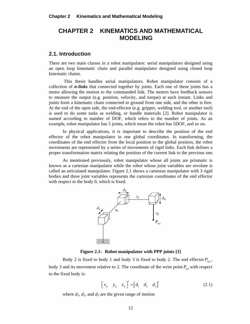
As mentioned previously, robot manipulator whose all joints are prismatic is known as a cartesian manipulator while the robot whose joint variables are revolute is called an articulated manipulator. Figure 2.1 shows a cartesian manipulator with 3 rigid bodies and three joint variables represents the cartesian coordinates of the end effector with respect to the body 0, which is fixed.
xyzP
Figure 2.1: Robot manipulator with PPP joints [1]
Body 2 is fixed to body 1 and body 3 is fixed to body 2. The end effector xyzP ,
body 3 and its movement relative to 2. The coordinate of the wrist point xyzP with respect
to the fixed body is:
1 2 3p p px y z d d d (2.1)
where d1, d2, and d3 are the given range of motion
Modeling and Control of 5DOF Robot Arm Using Supervisory Control
13
Kinematics is the motion geometry of the robot manipulator from the reference position to the desired position with no regard to forces or other factors that influence robot motion [3]. In other words, the kinematics deals with the movement of the robot manipulator with respect to fixed frame as a function of time. The fixed frame in robot represents the base and all other movements measured from the base as reference. It is one of the most fundamental disciplines in robots, providing tools for describing the structure and behavior of robot manipulator mechanisms, and it is important in practical applications such as trajectory planning and control purposes.
Generally, to control any robot manipulator the core of the controller is a description of kinematic analysis, this is done by using a common method in industrial and academic research, namely Denavit-Hartenberg method [1], [2] and [3]. The distinct of this method gives a mathematical description for all serial manipulators depending on the robot geometry, and it defines the position and orientation of the current link with respect to previous one. In addition, it allows the desired frame to create a set of steps to bring the other links coordinate into corresponding with another one. For more information, readers may return to the previous references. The kinematic solution in this chapter will focus on two important problem arises in robot manipulator. Section (2.2) discusses methodologies to solve the forward and inverse kinematic respectively.
The first problem is determining the forward kinematic (FK) where the robot manipulator end-effector will be if all joints are known. This means what rigid motion each joint effect on its link to obtain the desired configuration. The configuration space of the end-effector contains the transformation matrix T that relates the position and orientation of the end-effector. The following equation explains the forward kinematic problem.
1 2( , , , ) [ , , , ] n dF x y z R (2.2)
where 1 2, and n are the input variables, [ , , ] x y z are the desired position and
dR the desired rotation.
The second problem is determining the inverse kinematic (IK), which calculates the value of each joint variable if the desired position and orientation of end-effector are known. That means if the final link configuration is known, what is the possible configuration (e.g. solutions) of the robot manipulator to move the end effector of the robot arm to desired position and orientation in space. Inverse kinematic problem may express mathematically as follows:
1 2( , , , ) , , , nF x y z R (2.3)
For serial manipulators with revolute or prismatic joints the FK is derived using procedures such as the DH convention matrix [3], but in the parallel manipulator, the forward kinematic be not easy to be solved due to the complexity of the robot manipulator. Therefore, it may solved by using a set of nonlinear equations. On the other hand, solving the IK for parallel manipulator is easier than FK solution, and there are many solutions to achieve the desired task.
The second issue that will be discussed through Chapter 2 is the DC motor modeling. DC motor modeling is an important issue before designing a controller to know the system characteristics and its mathematical model.
Chapter 2 Kinematics and Mathematical Modeling
14
To have a good model, it is important to understand the system behavior and to solve the associated problems. In general, an accurate model means that a designer would be able to predict the action of the system, diagnoses failure and simulates it in a precise manner or controls it to go to the desired position. Section (2.3) presents modeling and analysis of DC motor to derive the motor speed and position transfer functions.
2.2. Kinematic Analysis
This section will discuss the main two problems in the robot manipulator kinematic: the forward and inverse kinematic respectively and develop general steps to obtain the kinematic equations for the configuration of any serial robot arm to determine the position and orientation of the end effector relative to the base.
2.2.1. Forward Kinematic
The forward kinematic equations, describe the functional relationship between the joint variables and the position and orientation of the end-effector. Suppose the robot has i-links, the joints and links numbered from 1 to i and 0 to i respectively. The joint variables are denoted by iq . In the case of prismatic joint, iq represents the displacement,
similarly iq represent the angle of rotation for the revolute joint.
Figure 1.1 illustrates the kinematic diagram and the frame assignment of a robot manipulator with n-DOF. We will derive the forward kinematics for i-links robot manipulator according to the DH convention.
Consider a fixed frame 0 0 0 0o x y z and the rotation frame 1 1 1 1o x y z . The orientation is
represented as a series of three revolute about a combination of the principle axes of the link frame. The rotation of the rotated frame about the fixed frame represented by the three angles , and . The first rotation about z axis by angle , and the next rotation about current y by angle and the third rotation about the current z axis by the angle .
According to [1] the rotational transformation matrix that represents the position of the frame i with respect to frame 0 is expressed in equation (2.4). This equation represents the rotation matrix of the ZYZ Euler angles:
, , ,
ZYZ Z Y ZR R R R
c c c s s c c s s c c s
s c c c c s c s c c s s
s c s s c
(2.4)
To obtain the forward kinematic equations the following steps should be done:
a) Obtain the DH parameters.
To describe the kinematics of any robot, four parameters are given for each link , , ,i i i ia d where two of them described the link, and the others describe the
connection with other links. In the case of revolute and prismatic robots, the variable i and id are denoted as joint variable. DH parameter is computed manually or
using computer programs such as MATHEMATICA or MATLAB programs. Table (2.1) shows the DH parameters for i-link robot manipulator.
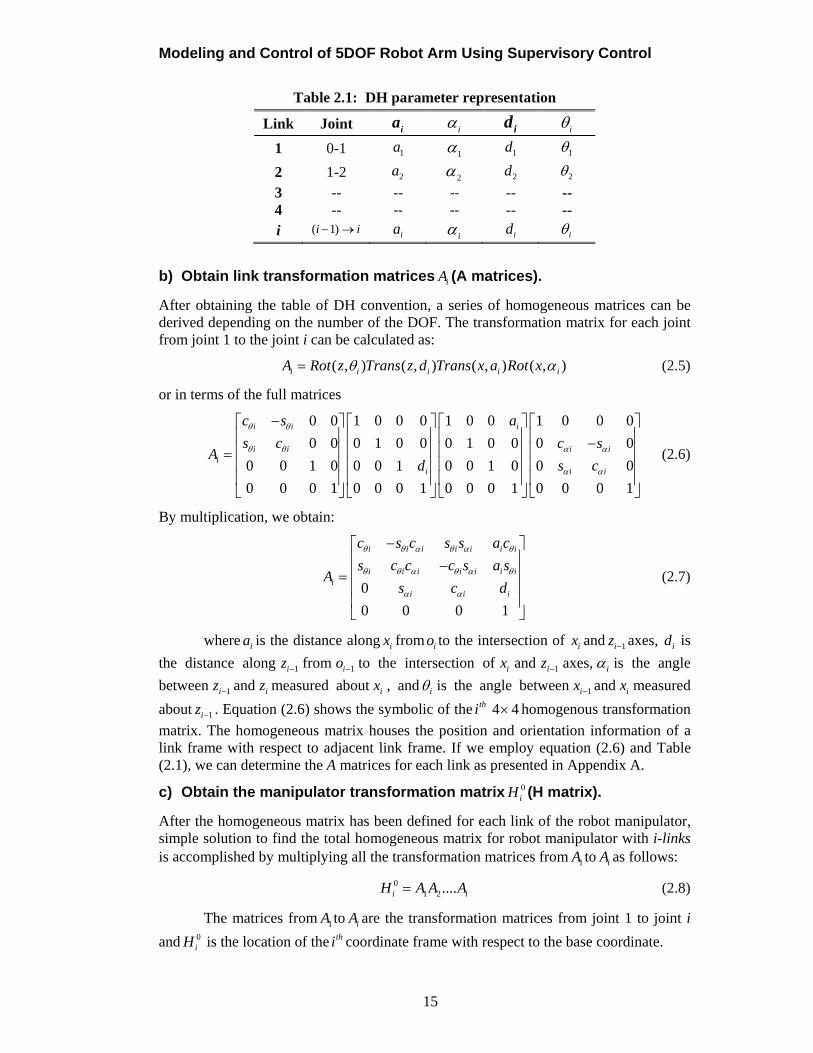
Modeling and Control of 5DOF Robot Arm Using Supervisory Control
15
Table 2.1: DH parameter representation
Link Joint ia i id i
1 0-1 1a 1 1d 1
2 1-2 2a 2 2d 2
3 -- -- -- -- -- 4 -- -- -- -- -- i ( 1)i i ia
i id i
b) Obtain link transformation matrices iA (A matrices).
After obtaining the table of DH convention, a series of homogeneous matrices can be derived depending on the number of the DOF. The transformation matrix for each joint from joint 1 to the joint i can be calculated as:
( , ) ( , ) ( , ) ( , )i i i i iA Rot z Trans z d Trans x a Rot x (2.5)
or in terms of the full matrices
0 0 1 0 0 0 1 0 0 1 0 0 0
0 0 0 1 0 0 0 1 0 0 0 0
0 0 1 0 0 0 1 0 0 1 0 0 0
0 0 0 1 0 0 0 1 0 0 0 1 0 0 0 1
i i i
i i i ii
i i i
c s a
s c c sA
d s c
(2.6)
By multiplication, we obtain:
0
0 0 0 1
i i i i i i i
i i i i i i ii
i i i
c s c s s a c
s c c c s a sA
s c d
(2.7)
where ia is the distance along ix from io to the intersection of ix and 1iz axes, id is
the distance along 1iz from 1io to the intersection of ix and 1iz axes, i is the angle
between 1iz and iz measured about ix , and i is the angle between 1ix and ix measured
about 1iz . Equation (2.6) shows the symbolic of the 4 4thi homogenous transformation
matrix. The homogeneous matrix houses the position and orientation information of a link frame with respect to adjacent link frame. If we employ equation (2.6) and Table (2.1), we can determine the A matrices for each link as presented in Appendix A.
c) Obtain the manipulator transformation matrix 0iH (H matrix).
After the homogeneous matrix has been defined for each link of the robot manipulator, simple solution to find the total homogeneous matrix for robot manipulator with i-links is accomplished by multiplying all the transformation matrices from 1A to iA as follows:
01 2....i iH A A A (2.8)
The matrices from 1A to iA are the transformation matrices from joint 1 to joint i
and 0iH is the location of the thi coordinate frame with respect to the base coordinate.

Chapter 2 Kinematics and Mathematical Modeling
16
d) Calculate the position and orientation of the end-effector.
The general homogeneous matrix for the desired position and orientation of the end-effector that obtained from Table (2.1) as follows:
11 12 13
21 22 2301 2
31 32 32
....
0 0 0 1
i i
r r r x
r r r yH A A A
r r r z
(2.9)
Equation (2.9) consists of two main components: the rotation matrix and the position vector of the end-effector as follows:
11 12 13
21 22 23
31 32 33
d
r r r
R r r r
r r r
(2.10)
x
P y
z
(2.11)
The orientation and the position of the end-effector solved directly once the homogeneous matrices for manipulator with i-links are multiplied.
The 3 3 rotation matrix provides the orientation of frame i with respect to the base frame. The position vector ( , , )Td x y z represents the desired position from the
origin 0o to the origin 1o expressed in the frame 0 0 0 0o x y z . In the previous equations
1 11 21 31( , , )Tc r r r is a vector represents the direction of ix in the 0 0 0 0o x y z system,
2 12 22 32( , , )Tc r r r is a vector represents the direction of iy , and 3 13 23 33( , , )Tc r r r represents
the direction of iz .
Solutions of the Euler angles are given as:
233 33tan 2( , 1 )A r r (2.12)
or
233 33tan 2( , 1 )A r r (2.13)
If 0s then:
13 23tan 2( , )A r r (2.14)
13 32tan 2( , )A r r (2.15)
If the value of 0s is chosen, then
13 23tan 2( , )A r r (2.16)
31 32tan 2( , )A r r (2.17)
Modeling and Control of 5DOF Robot Arm Using Supervisory Control
17
2.2.2. Inverse Kinematic
This section is concerned with the IK problem to find the joint variables of the robot manipulator for a given position and orientation of the end effector [1]. The problem of the inverse kinematics (IK) is more difficult than the forward kinematics problem. It can be mathematically expressed as:
( , , , , , )k kf x y z (2.18)
where 1, ,k i , k joint angles and ( , , , , , )x y z represents the position and
orientation.
There are steps used to solve the inverse kinematics for robot manipulator as follows:
1. Equate the general transformation matrix to the final transformation matrix of the robot manipulator.
11 12 13
0 21 22 231 2
31 32 33
0 0 0 1
....i i
r r r xr r r yr r r z
H A A A
(2.19)
2. For the both matrices define: a) The elements that contain one joint variable. b) Pairs of elements, which contain only one joint variable. c) Elements, or combinations of elements, contain more than one joint variable.
3. After defining these elements, equate it to the corresponding elements in the other matrix to form equations, and then solve these equations to find the values of joint variables.
4. Repeat step (3) to identify all elements in the two matrices. 5. In the case of inaccuracy, solutions look for another one. 6. If there is more joint variable to be found, multiply equation (2.19) by the inverse of
A matrix for the specified links. 7. Repeat steps (2) through (6) until solution to all joint variables have been found. 8. If there is no solution to the joint variable in terms of an element transformation
matrix, it means that the arm cannot achieve the specified position and orientation; the position is outside the robot manipulator workspace.
Calculation of the inverse of iA matrices and solution of the inverse kinematics
for joint variables of the experimental robot are derived in Appendix A.
2.3. DC Motor Modeling
Generally, modeling refers to system (e.g. plant) description in mathematical terms, which characterizes the input-output relationship [39]. Direct current (DC) motor is a common actuator found in many mechanical systems and industrial applications such as industrial and educational robots [3]. DC motor converts the electrical energy to mechanical energy. The motor directly has a rotary motion, and when combined with mechanical part it can provide translation motion for the desired link.
Equation (2.20) states the relation between the current and developed torque in the motor shaft.
( ) ( )m m at K i t (2.20)
Chapter 2 Kinematics and Mathematical Modeling
18
where ( )m t , is the motor torque produced by the motor shaft, , the magnetic
flux, ( )ai t , the armature current, and mK , is a proportional constant.
Equation (2.21) illustrates the relation between the produced EMF and the shaft velocity:
( )b m mv t K (2.21)
where ( )bv t , denotes the back EMF, and m , is the shaft velocity of the motor.
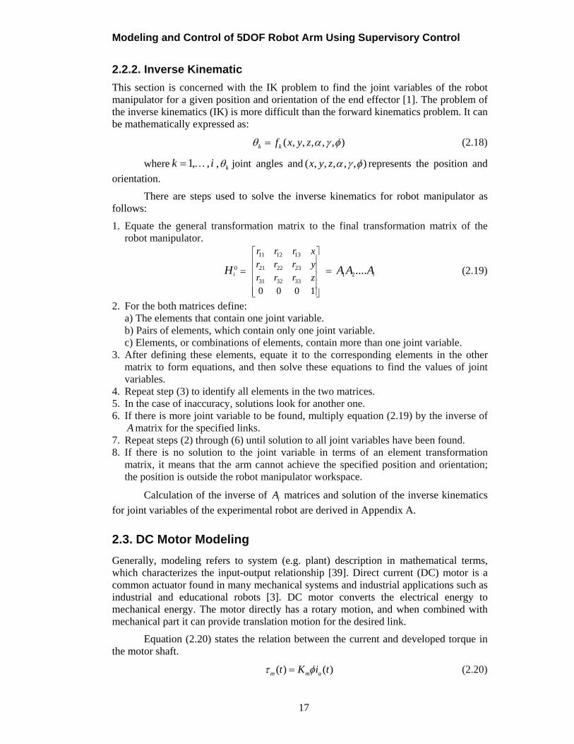
DC motors are important in control systems, so it is necessary to establish and analyze the mathematical model of the DC motors [39]. Figure 2.2 shows the schematic of the armature controlled DC motor with a fixed field circuit.
( )av t ( )bv t
aLaR
Figure 2.2: Schematic of DC motor system
It is modeled as circuit with resistance and inductance connected in series. The input voltage ( )av t , is the voltage supplied by amplifier to move the motor. The back
EMF voltage ( )bv t , is induced by the rotation of the armature windings in the fixed
magnetic field. To derive the transfer function of the DC motor, the system is divided into three major components of equation: electrical equation, mechanical equation, and electro-mechanical equation [28]. Equation (2.22) and (2.23) are derived in Appendix A. The transfer function of the motor speed is:
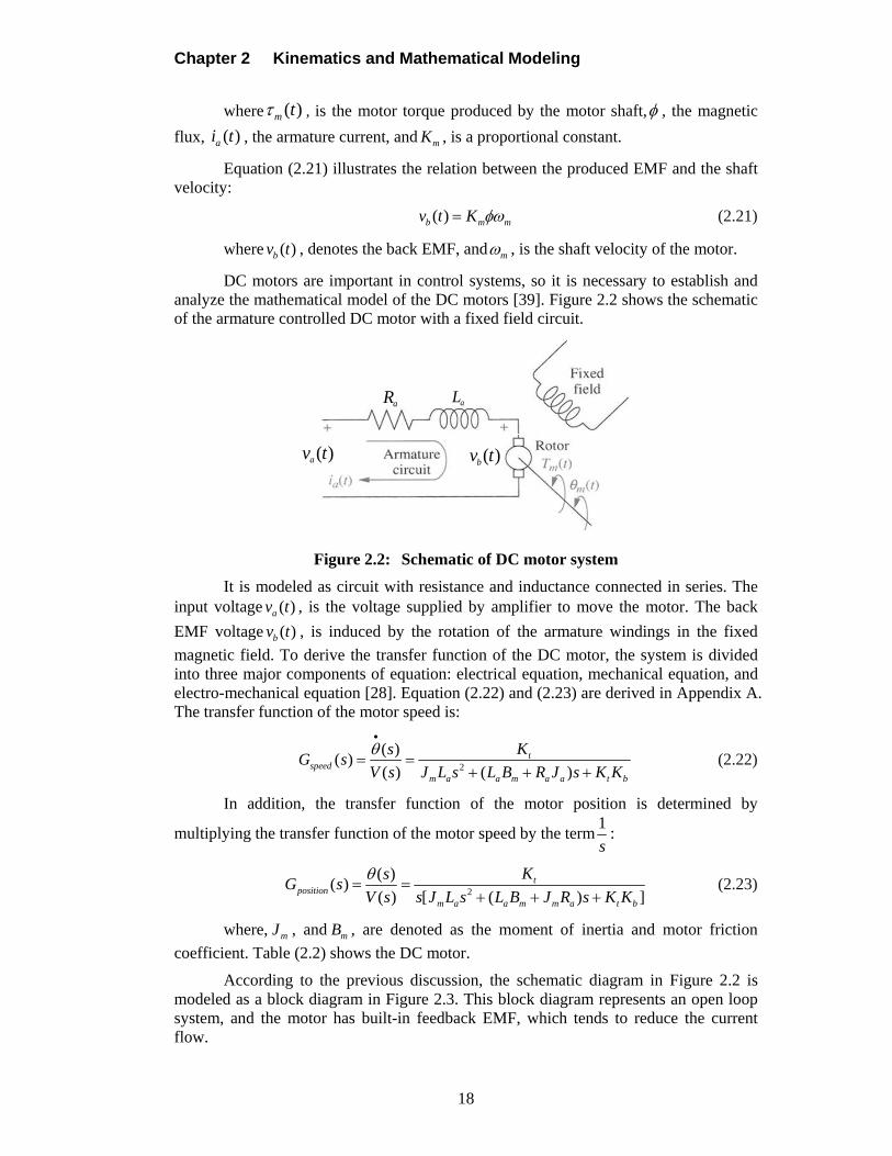
2
( )( )
( ) ( )t
speedm a a m a a t b
KsG s
V s J L s L B R J s K K
(2.22)
In addition, the transfer function of the motor position is determined by
multiplying the transfer function of the motor speed by the term1
s:
2
( )( )
( ) [ ( ) ]t
positionm a a m m a t b
KsG s
V s s J L s L B J R s K K
(2.23)
where, mJ , and mB , are denoted as the moment of inertia and motor friction
coefficient. Table (2.2) shows the DC motor.
According to the previous discussion, the schematic diagram in Figure 2.2 is modeled as a block diagram in Figure 2.3. This block diagram represents an open loop system, and the motor has built-in feedback EMF, which tends to reduce the current flow.
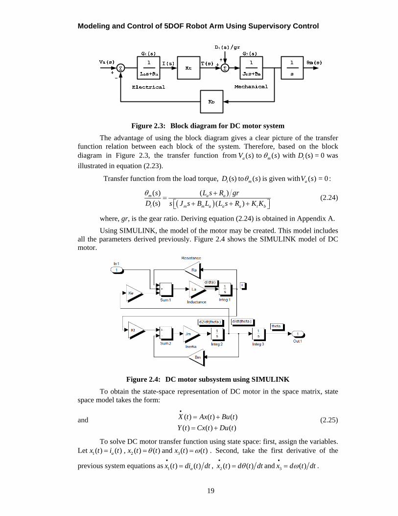
Modeling and Control of 5DOF Robot Arm Using Supervisory Control
19
Figure 2.3: Block diagram for DC motor system
The advantage of using the block diagram gives a clear picture of the transfer function relation between each block of the system. Therefore, based on the block diagram in Figure 2.3, the transfer function from ( )aV s to ( )m s with (s) = 0tD was
illustrated in equation (2.23).
Transfer function from the load torque, (s)tD to ( )m s is given with ( ) = 0aV s :
( ) ( )
(s) ( )m a a
t m m a a a t b
s L s R gr
D s J s B L L s R K K
(2.24)
where, gr, is the gear ratio. Deriving equation (2.24) is obtained in Appendix A.
Using SIMULINK, the model of the motor may be created. This model includes all the parameters derived previously. Figure 2.4 shows the SIMULINK model of DC motor.
Figure 2.4: DC motor subsystem using SIMULINK
To obtain the state-space representation of DC motor in the space matrix, state space model takes the form:
and ( ) ( ) ( )
( ) ( ) ( )
X t Ax t Bu t
Y t Cx t Du t
(2.25)
To solve DC motor transfer function using state space: first, assign the variables. Let 1( ) ( )ax t i t , 2 ( ) ( )x t t and 3( ) ( )x t t . Second, take the first derivative of the
previous system equations as 1( ) ( )ax t di t dt
, 2 ( ) ( )x t d t dt
and 3 ( )x d t dt
.
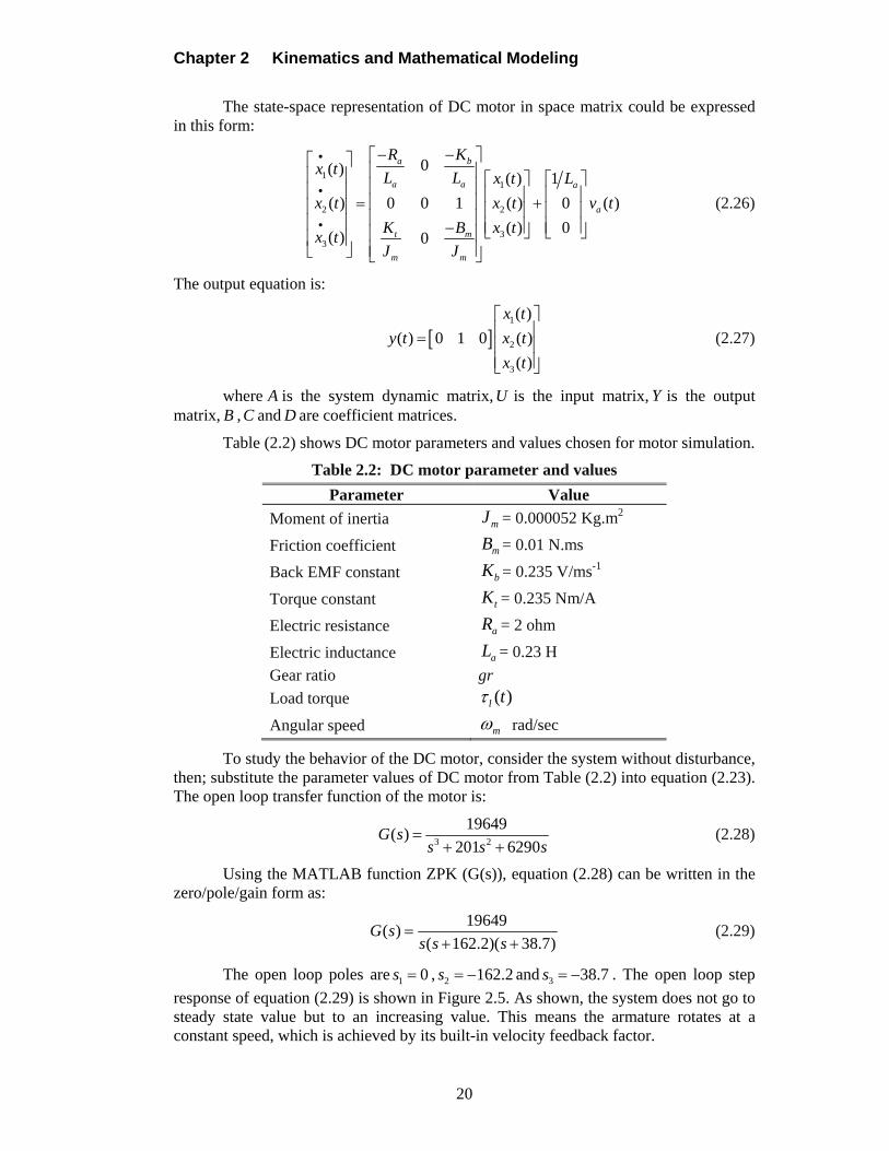
Chapter 2 Kinematics and Mathematical Modeling
20
The state-space representation of DC motor in space matrix could be expressed in this form:
11
2 2
33
0( )( ) 1
( ) 0 0 1 ( ) 0 ( )
( ) 0( ) 0
a b
a a a
a
t m
m m
R Kx t L L x t L
x t x t v t
K B x tx t
J J
(2.26)
The output equation is:
1
2
3
( )
( ) 0 1 0 ( )
( )
x t
y t x t
x t
(2.27)
where A is the system dynamic matrix, U is the input matrix, Y is the output matrix, B , C and D are coefficient matrices.
Table (2.2) shows DC motor parameters and values chosen for motor simulation.
Table 2.2: DC motor parameter and values
Parameter Value
Moment of inertia mJ = 0.000052 Kg.m2
Friction coefficient mB = 0.01 N.ms
Back EMF constant bK = 0.235 V/ms-1
Torque constant tK = 0.235 Nm/A
Electric resistance aR = 2 ohm
Electric inductance aL = 0.23 H
Gear ratio gr
Load torque ( )l t
Angular speed m rad/sec
To study the behavior of the DC motor, consider the system without disturbance, then; substitute the parameter values of DC motor from Table (2.2) into equation (2.23). The open loop transfer function of the motor is:
3 2
19649(
2)
201 6 90s sG
ss
(2.28)
Using the MATLAB function ZPK (G(s)), equation (2.28) can be written in the zero/pole/gain form as:
( 162.2)( 38.
1964( )
)
9
7G s
s s s (2.29)
The open loop poles are 1 0s , 2 162.2s and 3 38.7s . The open loop step
response of equation (2.29) is shown in Figure 2.5. As shown, the system does not go to steady state value but to an increasing value. This means the armature rotates at a constant speed, which is achieved by its built-in velocity feedback factor.
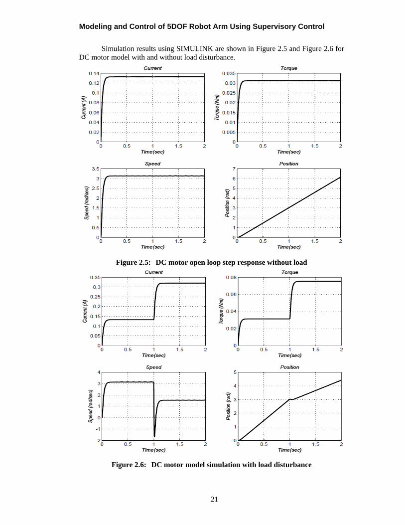
Modeling and Control of 5DOF Robot Arm Using Supervisory Control
21
Simulation results using SIMULINK are shown in Figure 2.5 and Figure 2.6 for DC motor model with and without load disturbance.
Figure 2.5: DC motor open loop step response without load
Figure 2.6: DC motor model simulation with load disturbance
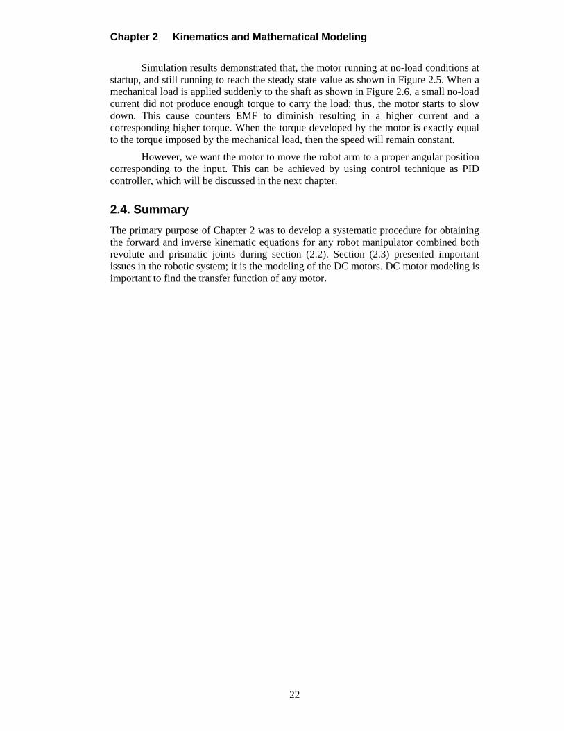
Chapter 2 Kinematics and Mathematical Modeling
22
Simulation results demonstrated that, the motor running at no-load conditions at startup, and still running to reach the steady state value as shown in Figure 2.5. When a mechanical load is applied suddenly to the shaft as shown in Figure 2.6, a small no-load current did not produce enough torque to carry the load; thus, the motor starts to slow down. This cause counters EMF to diminish resulting in a higher current and a corresponding higher torque. When the torque developed by the motor is exactly equal to the torque imposed by the mechanical load, then the speed will remain constant.
However, we want the motor to move the robot arm to a proper angular position corresponding to the input. This can be achieved by using control technique as PID controller, which will be discussed in the next chapter.
2.4. Summary
The primary purpose of Chapter 2 was to develop a systematic procedure for obtaining the forward and inverse kinematic equations for any robot manipulator combined both revolute and prismatic joints during section (2.2). Section (2.3) presented important issues in the robotic system; it is the modeling of the DC motors. DC motor modeling is important to find the transfer function of any motor.
Modeling and Control of 5DOF Robot Arm Using Supervisory Control
23
CHAPTER 3 PID CONTROLLER DESIGN
3.1. Introduction
PID controller is considered the most control technique that is widely used in control applications. A huge number of applications and control engineers had used the PID controller in daily life. On the other hand, many research papers, number of master and doctoral theses and books have been written on this subject. PID control offers an easy method of controlling a process by varying its parameters. PID works well in industrial applications such as slow industrial manipulators were large components of joint inertia added by actuators. Since the invention of PID control in 1910, and Ziegler-Nichols’ (ZN) tuning method in 1942 [7] and [38], PID controllers became dominant and popular issues in control theory due to simplicity of implementation, simplicity of design, and the ability to be used in a wide range of applications [40]. Moreover, they are available at low cost. Finally, it provides robust and reliable performance for most systems if the parameters are tuned properly. According to different sources like JEMIMA2, PID controllers or PID variations (P, PD, and PI) are widely used in more than 90% to 95% of control applications. However, the PID controller has its own limitation; the PID performances can give only satisfactory performance if the requirement is reasonable and the process parameters variation are limited.
Setting the PID parameters is called tuning. During the last six decades, several methods have been proposed for determining the PID controller gains. Some of those methods use the information concerning the open loop characteristics such as Cohen-Coon method. Other methods use the Nyquist curve plotting of the plant such as Ziegler-Nichols tuning method [41]. All of these tuning formulas need to know a prior knowledge about the system. PID control technique is used to control and enhance the system characteristics such as reducing the overshoot, speed up rising time, and eliminating the steady state error. Each one of the PID parameters has specific criteria to enhance the characteristics of the controlled system. These specifications will be discussed through this chapter, and the result will be presented and included in Chapter 6.
3.2. PID Structure
PID algorithm, assumes the controlled plant is known, such as a robot manipulator [17]. As shown in Figure 1.2, the error signal, ( )e t , is the difference between the set point,
( )r t , and the process output, ( )y t . If the error between the output and the input values is large, then large input signal is applied to the physical system. If the error is small, a small input signal is used. As its name suggested, any change in the control signal, ( )u t
is directly proportional to change in the error signal for a given proportional gain PK .
Mathematically the output of the proportional controller is given as follows:
( ) ( )Pu t K e t (3.1)
where ( )e t , the error signal and ( ) ( )PK u t e t indicates the change of the output
signal to the change of the error signal. 2 Japan Electric Measuring Instrument Manufacture’s Association
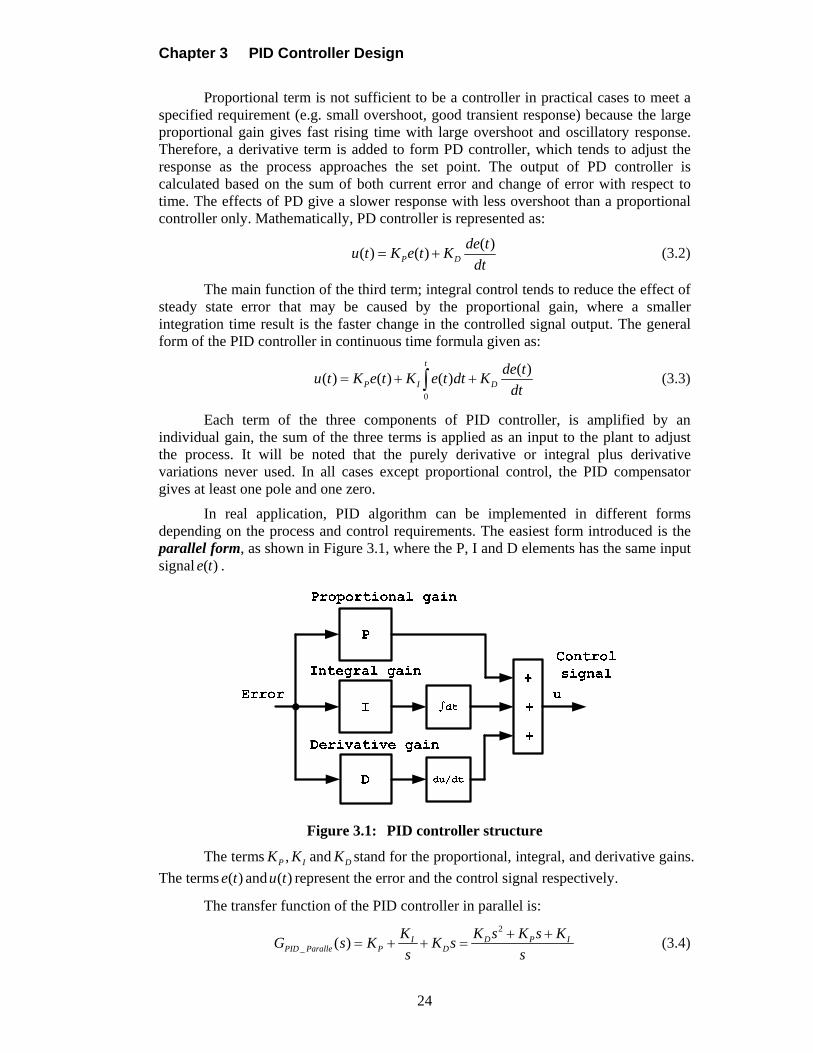
Chapter 3 PID Controller Design
24
Proportional term is not sufficient to be a controller in practical cases to meet a specified requirement (e.g. small overshoot, good transient response) because the large proportional gain gives fast rising time with large overshoot and oscillatory response. Therefore, a derivative term is added to form PD controller, which tends to adjust the response as the process approaches the set point. The output of PD controller is calculated based on the sum of both current error and change of error with respect to time. The effects of PD give a slower response with less overshoot than a proportional controller only. Mathematically, PD controller is represented as:
( )
( ) ( )P D
de tu t K e t K
dt (3.2)
The main function of the third term; integral control tends to reduce the effect of steady state error that may be caused by the proportional gain, where a smaller integration time result is the faster change in the controlled signal output. The general form of the PID controller in continuous time formula given as:
0
( )( ) ( ) ( )
t
P I D
de tu t K e t K e t dt K
dt (3.3)
Each term of the three components of PID controller, is amplified by an individual gain, the sum of the three terms is applied as an input to the plant to adjust the process. It will be noted that the purely derivative or integral plus derivative variations never used. In all cases except proportional control, the PID compensator gives at least one pole and one zero.
In real application, PID algorithm can be implemented in different forms depending on the process and control requirements. The easiest form introduced is the parallel form, as shown in Figure 3.1, where the P, I and D elements has the same input signal ( )e t .
Figure 3.1: PID controller structure
The terms ,P IK K and DK stand for the proportional, integral, and derivative gains.
The terms ( )e t and ( )u t represent the error and the control signal respectively.
The transfer function of the PID controller in parallel is:
2
_ ( ) I D P IPID Paralle P D
K K s K s KG s K K s
s s
(3.4)
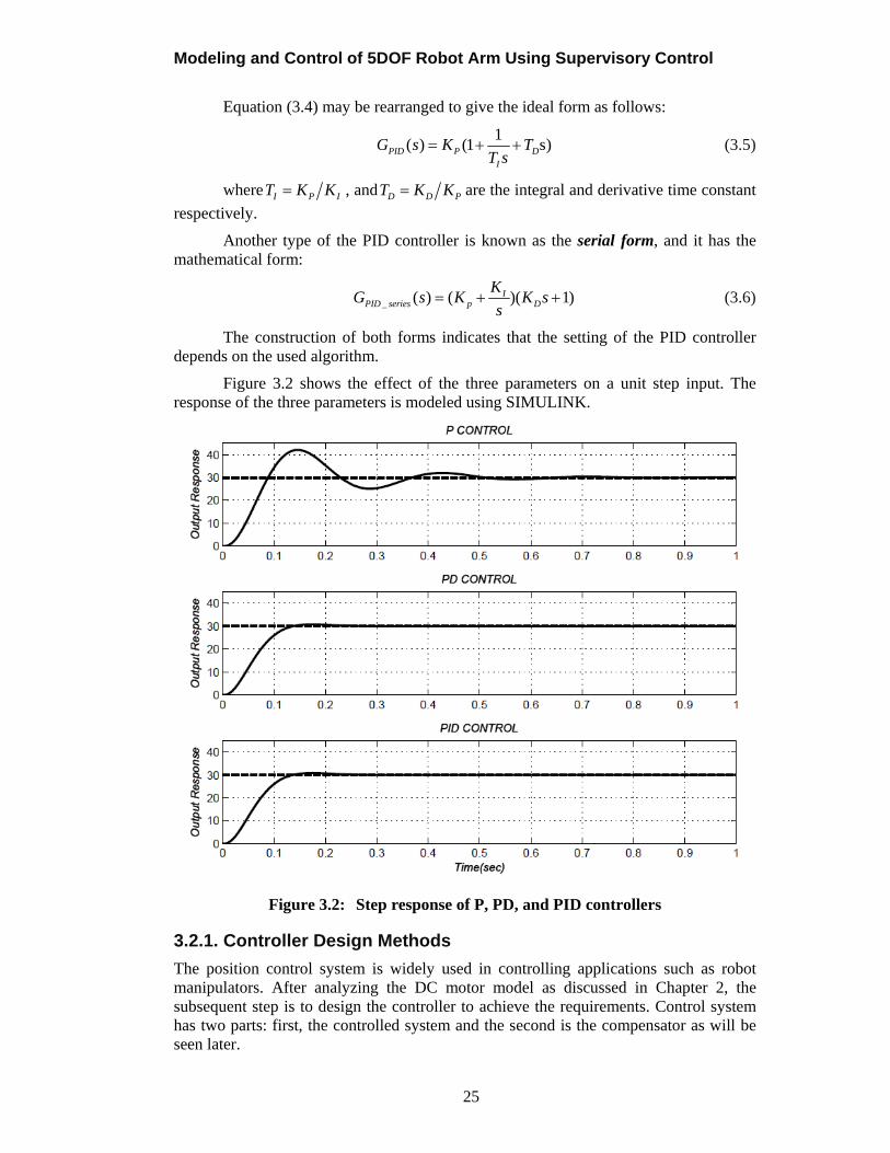
Modeling and Control of 5DOF Robot Arm Using Supervisory Control
25
Equation (3.4) may be rearranged to give the ideal form as follows:
1
( ) (1 s)PID P DI
G s K TT s
(3.5)
where I P IT K K , and D D PT K K are the integral and derivative time constant
respectively.
Another type of the PID controller is known as the serial form, and it has the mathematical form:
_ ( ) ( )( 1)IPID series p D
KG s K K s
s (3.6)
The construction of both forms indicates that the setting of the PID controller depends on the used algorithm.
Figure 3.2 shows the effect of the three parameters on a unit step input. The response of the three parameters is modeled using SIMULINK.
Figure 3.2: Step response of P, PD, and PID controllers
3.2.1. Controller Design Methods
The position control system is widely used in controlling applications such as robot manipulators. After analyzing the DC motor model as discussed in Chapter 2, the subsequent step is to design the controller to achieve the requirements. Control system has two parts: first, the controlled system and the second is the compensator as will be seen later.
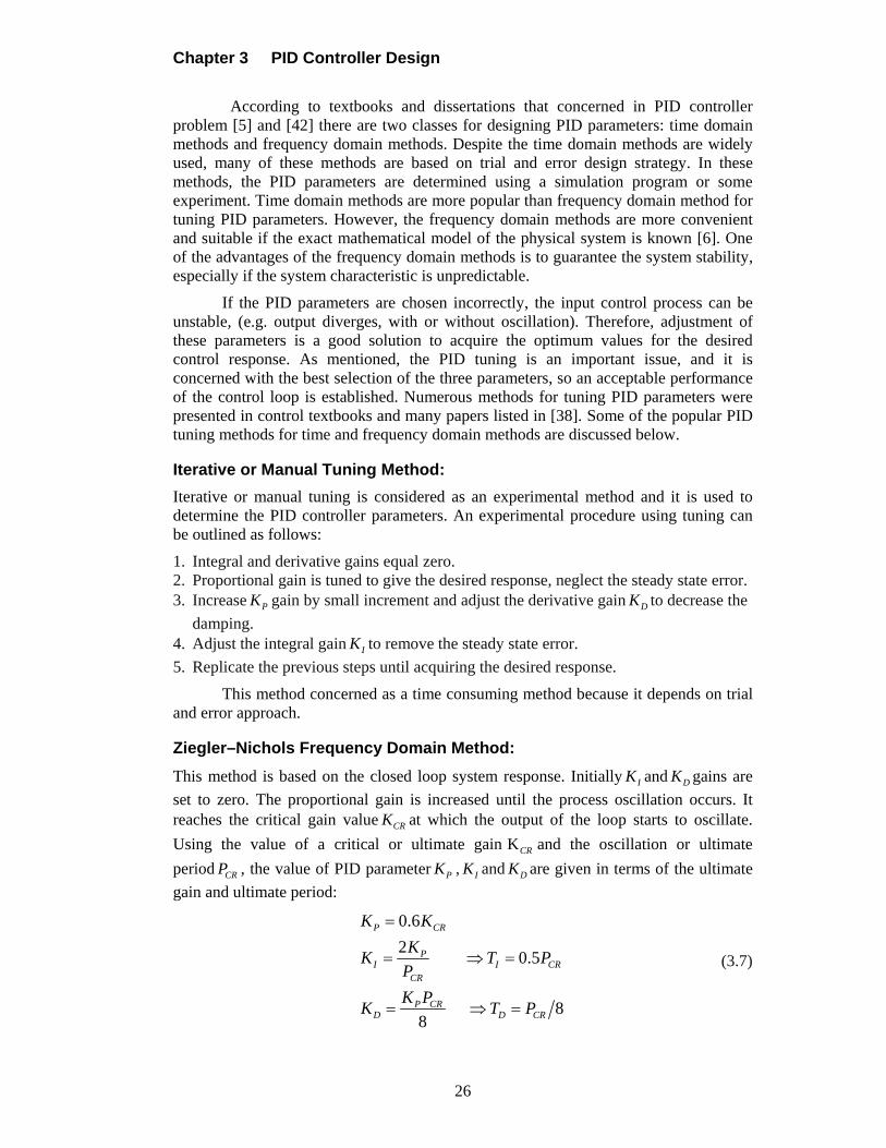
Chapter 3 PID Controller Design
26
According to textbooks and dissertations that concerned in PID controller problem [5] and [42] there are two classes for designing PID parameters: time domain methods and frequency domain methods. Despite the time domain methods are widely used, many of these methods are based on trial and error design strategy. In these methods, the PID parameters are determined using a simulation program or some experiment. Time domain methods are more popular than frequency domain method for tuning PID parameters. However, the frequency domain methods are more convenient and suitable if the exact mathematical model of the physical system is known [6]. One of the advantages of the frequency domain methods is to guarantee the system stability, especially if the system characteristic is unpredictable.
If the PID parameters are chosen incorrectly, the input control process can be unstable, (e.g. output diverges, with or without oscillation). Therefore, adjustment of these parameters is a good solution to acquire the optimum values for the desired control response. As mentioned, the PID tuning is an important issue, and it is concerned with the best selection of the three parameters, so an acceptable performance of the control loop is established. Numerous methods for tuning PID parameters were presented in control textbooks and many papers listed in [38]. Some of the popular PID tuning methods for time and frequency domain methods are discussed below.
Iterative or Manual Tuning Method:
Iterative or manual tuning is considered as an experimental method and it is used to determine the PID controller parameters. An experimental procedure using tuning can be outlined as follows:
1. Integral and derivative gains equal zero. 2. Proportional gain is tuned to give the desired response, neglect the steady state error. 3. Increase PK gain by small increment and adjust the derivative gain DK to decrease the
damping. 4. Adjust the integral gain IK to remove the steady state error.
5. Replicate the previous steps until acquiring the desired response.
This method concerned as a time consuming method because it depends on trial and error approach.
Ziegler–Nichols Frequency Domain Method:
This method is based on the closed loop system response. Initially IK and DK gains are
set to zero. The proportional gain is increased until the process oscillation occurs. It reaches the critical gain value CRK at which the output of the loop starts to oscillate.
Using the value of a critical or ultimate gain KCR and the oscillation or ultimate
period CRP , the value of PID parameter PK , IK and DK are given in terms of the ultimate
gain and ultimate period:
0.6
2 0.5
88
P CR
PI I CR
CR
P CRD D CR
K K
KK T P
P
K PK T P
(3.7)
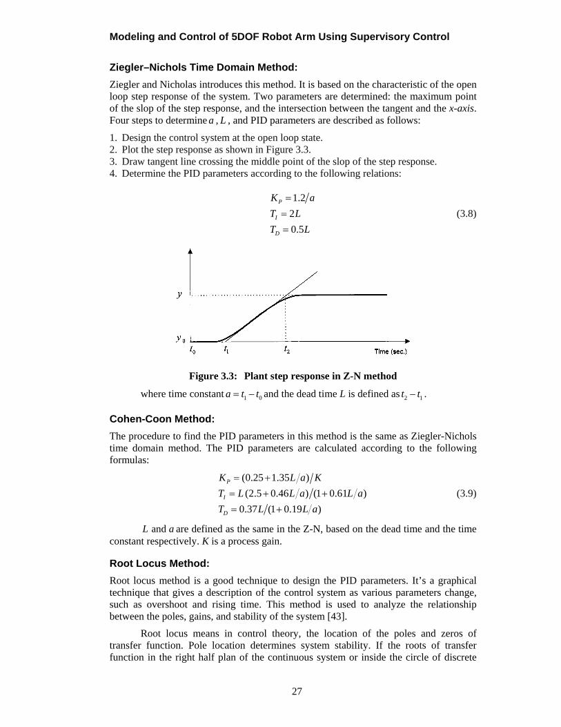
Modeling and Control of 5DOF Robot Arm Using Supervisory Control
27
Ziegler–Nichols Time Domain Method:
Ziegler and Nicholas introduces this method. It is based on the characteristic of the open loop step response of the system. Two parameters are determined: the maximum point of the slop of the step response, and the intersection between the tangent and the x-axis. Four steps to determine a , L , and PID parameters are described as follows:
1. Design the control system at the open loop state. 2. Plot the step response as shown in Figure 3.3. 3. Draw tangent line crossing the middle point of the slop of the step response. 4. Determine the PID parameters according to the following relations:
1.2
2
0.5
P
I
D
K a
T L
T L
(3.8)
Figure 3.3: Plant step response in Z-N method
where time constant 1 0a t t and the dead time L is defined as 2 1t t .
Cohen-Coon Method:
The procedure to find the PID parameters in this method is the same as Ziegler-Nichols time domain method. The PID parameters are calculated according to the following formulas:
(0.25 1.35 )
(2.5 0.46 ) (1 0.61 )
0.37 (1 0.19 )
P
I
D
K L a K
T L L a L a
T L L a
(3.9)
and L a are defined as the same in the Z-N, based on the dead time and the time constant respectively. K is a process gain.
Root Locus Method:
Root locus method is a good technique to design the PID parameters. It’s a graphical technique that gives a description of the control system as various parameters change, such as overshoot and rising time. This method is used to analyze the relationship between the poles, gains, and stability of the system [43].
Root locus means in control theory, the location of the poles and zeros of transfer function. Pole location determines system stability. If the roots of transfer function in the right half plan of the continuous system or inside the circle of discrete
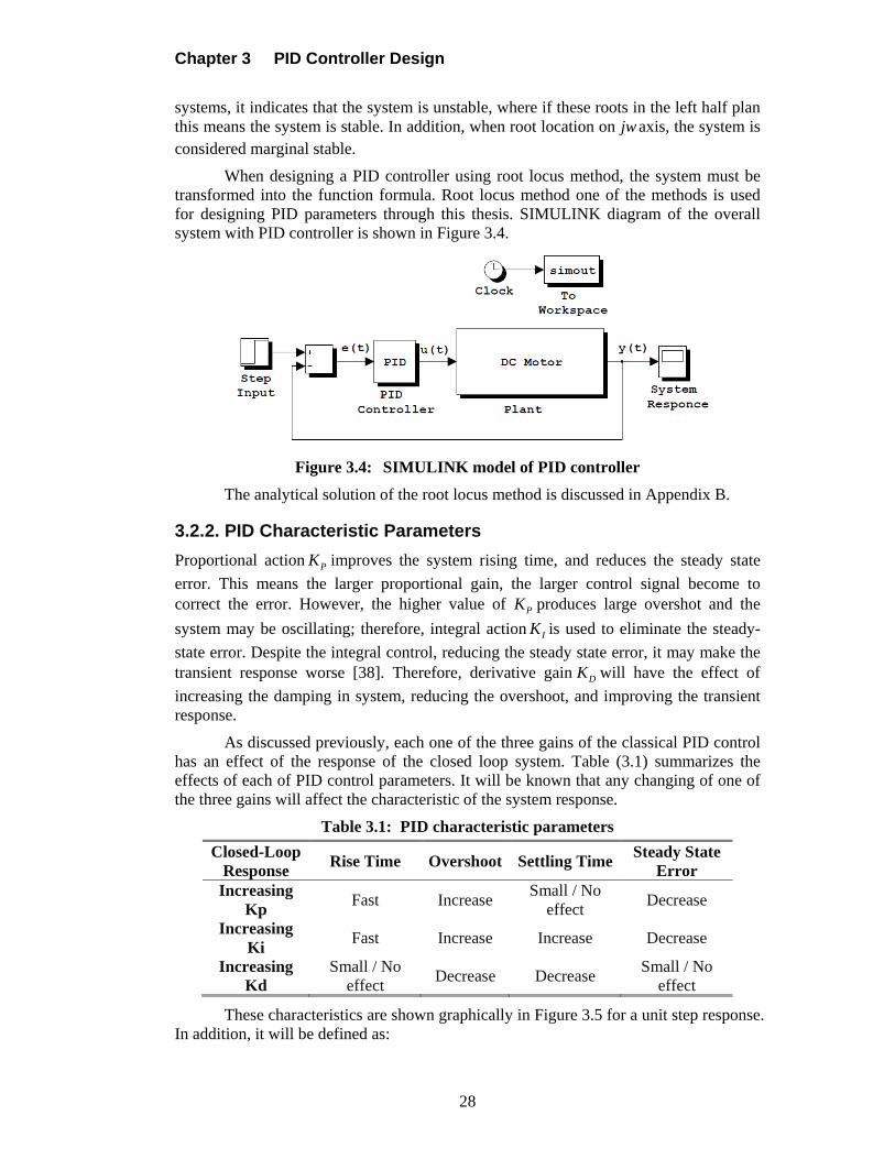
Chapter 3 PID Controller Design
28
systems, it indicates that the system is unstable, where if these roots in the left half plan this means the system is stable. In addition, when root location on jw axis, the system is considered marginal stable.
When designing a PID controller using root locus method, the system must be transformed into the function formula. Root locus method one of the methods is used for designing PID parameters through this thesis. SIMULINK diagram of the overall system with PID controller is shown in Figure 3.4.
Figure 3.4: SIMULINK model of PID controller
The analytical solution of the root locus method is discussed in Appendix B.
3.2.2. PID Characteristic Parameters
Proportional action PK improves the system rising time, and reduces the steady state
error. This means the larger proportional gain, the larger control signal become to correct the error. However, the higher value of PK produces large overshot and the
system may be oscillating; therefore, integral action IK is used to eliminate the steady-
state error. Despite the integral control, reducing the steady state error, it may make the transient response worse [38]. Therefore, derivative gain DK will have the effect of
increasing the damping in system, reducing the overshoot, and improving the transient response.
As discussed previously, each one of the three gains of the classical PID control has an effect of the response of the closed loop system. Table (3.1) summarizes the effects of each of PID control parameters. It will be known that any changing of one of the three gains will affect the characteristic of the system response.
Table 3.1: PID characteristic parameters
Closed-Loop Response
Rise Time Overshoot Settling Time Steady State
Error Increasing
Kp Fast Increase
Small / No effect
Decrease
Increasing Ki
Fast Increase Increase Decrease
Increasing Kd
Small / No effect
Decrease Decrease Small / No
effect
These characteristics are shown graphically in Figure 3.5 for a unit step response. In addition, it will be defined as:
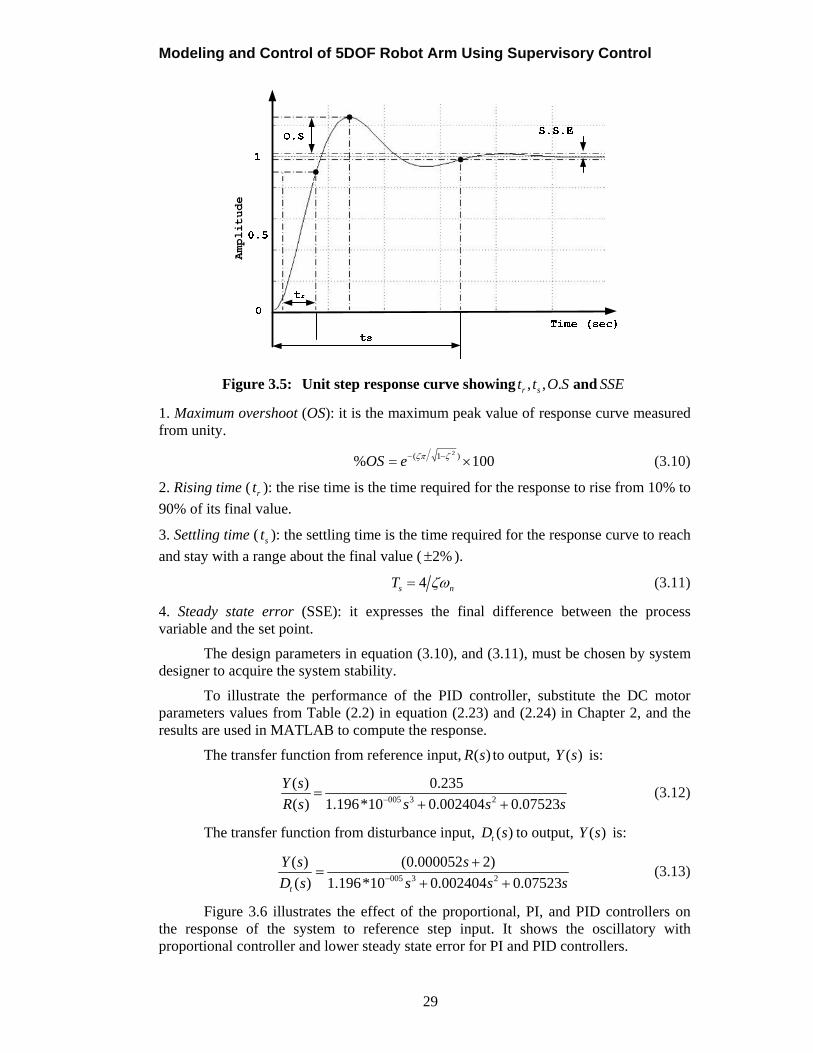
Modeling and Control of 5DOF Robot Arm Using Supervisory Control
29
Am
pl
it
ud
e
Figure 3.5: Unit step response curve showing , , .r st t O S and SSE
1. Maximum overshoot (OS): it is the maximum peak value of response curve measured from unity.
2( 1 )% 100OS e (3.10)
2. Rising time ( rt ): the rise time is the time required for the response to rise from 10% to
90% of its final value.
3. Settling time ( st ): the settling time is the time required for the response curve to reach
and stay with a range about the final value ( 2% ).
4s nT (3.11)
4. Steady state error (SSE): it expresses the final difference between the process variable and the set point.
The design parameters in equation (3.10), and (3.11), must be chosen by system designer to acquire the system stability.
To illustrate the performance of the PID controller, substitute the DC motor parameters values from Table (2.2) in equation (2.23) and (2.24) in Chapter 2, and the results are used in MATLAB to compute the response.
The transfer function from reference input, ( )R s to output, ( )Y s is:
005 3 21.196*10 0.002404 0.07
( ) 0.235
( ) 523
Y s
s sR s s (3.12)
The transfer function from disturbance input, ( )tD s to output, ( )Y s is:
005 3 21.196*
( )
10 0.002404 0.0
(0.0
7523
00052 2)
( )t s
Y s s
sD s s
(3.13)
Figure 3.6 illustrates the effect of the proportional, PI, and PID controllers on the response of the system to reference step input. It shows the oscillatory with proportional controller and lower steady state error for PI and PID controllers.
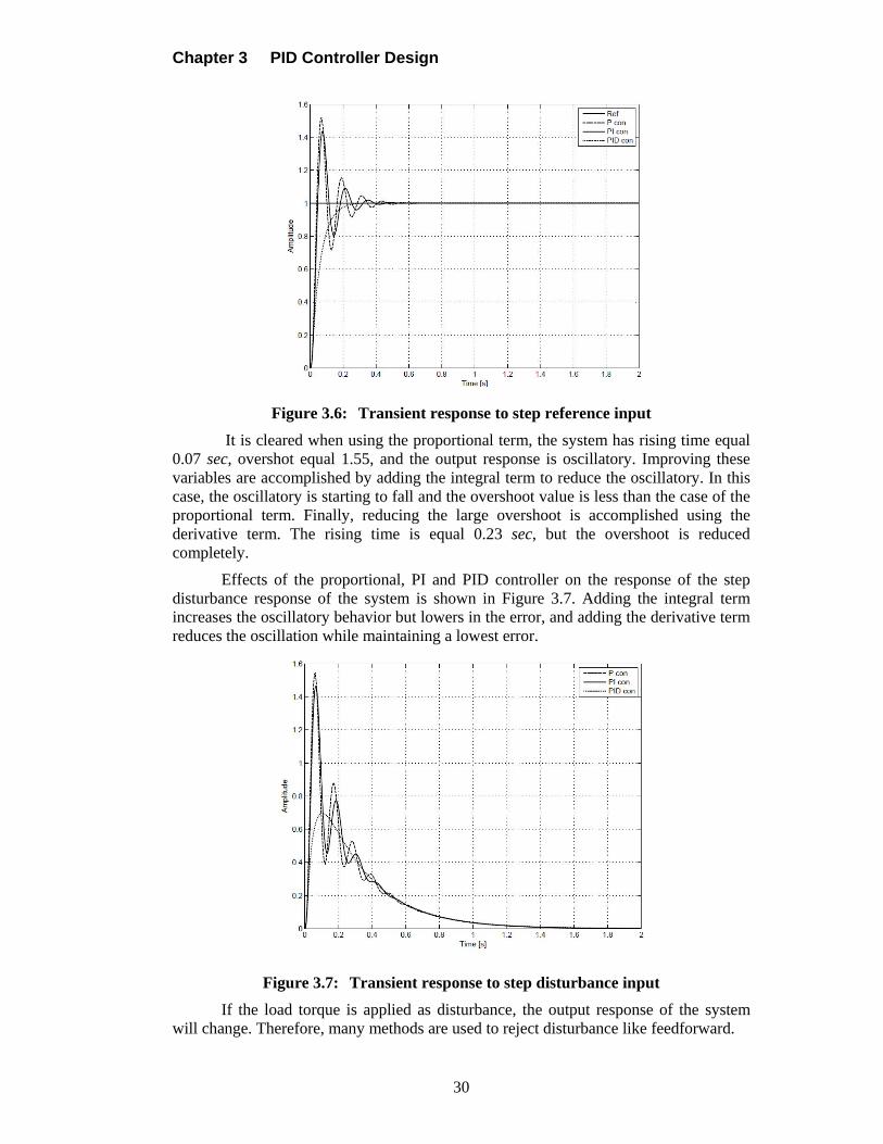
Chapter 3 PID Controller Design
30
Figure 3.6: Transient response to step reference input
It is cleared when using the proportional term, the system has rising time equal 0.07 sec, overshot equal 1.55, and the output response is oscillatory. Improving these variables are accomplished by adding the integral term to reduce the oscillatory. In this case, the oscillatory is starting to fall and the overshoot value is less than the case of the proportional term. Finally, reducing the large overshoot is accomplished using the derivative term. The rising time is equal 0.23 sec, but the overshoot is reduced completely.
Effects of the proportional, PI and PID controller on the response of the step disturbance response of the system is shown in Figure 3.7. Adding the integral term increases the oscillatory behavior but lowers in the error, and adding the derivative term reduces the oscillation while maintaining a lowest error.
Figure 3.7: Transient response to step disturbance input
If the load torque is applied as disturbance, the output response of the system will change. Therefore, many methods are used to reject disturbance like feedforward.
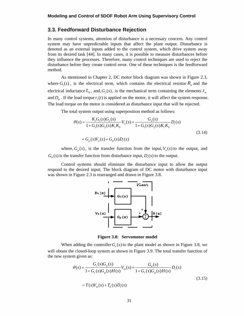
Modeling and Control of 5DOF Robot Arm Using Supervisory Control
31
3.3. Feedforward Disturbance Rejection
In many control systems, attention of disturbance is a necessary concern. Any control system may have unpredictable inputs that affect the plant output. Disturbance is denoted as an external inputs added to the control system, which drive system away from its desired task [44]. In many cases, it is possible to measure disturbances before they influence the processes. Therefore, many control techniques are used to reject the disturbance before they create control error. One of these techniques is the feedforward method.
As mentioned in Chapter 2, DC motor block diagram was shown in Figure 2.3, where 1( )G s , is the electrical term, which contains the electrical resistor aR and the
electrical inductance aL , and, 2 ( )G s , is the mechanical term containing the elements mJ
and mD . If the load torque ( )l t is applied on the motor, it will affect the system response.
The load torque on the motor is considered as disturbance input that will be rejected.
The total system output using superposition method as follows:
1 2 2
1 2 1 2
( ) ( ) ( )( ) ( ) ( )
1 ( ) ( ) 1 ( ) ( )
( ) ( ) ( ) ( )
ta t
t b t b
p a d t
K G s G s G ss V s D s
G s G s K K G s G s K K
G s V s G s D s
(3.14)
where, ( )pG s , is the transfer function from the input, ( )aV s to the output, and
( )dG s is the transfer function from disturbance input, ( )tD s to the output.
Control systems should eliminate the disturbance input to allow the output respond to the desired input; The block diagram of DC motor with disturbance input was shown in Figure 2.3 is rearranged and drawn in Figure 3.8.
Figure 3.8: Servomotor model
When adding the controller ( )cG s to the plant model as shown in Figure 3.8, we
will obtain the closed-loop system as shown in Figure 3.9. The total transfer function of the new system given as:
( ) ( ) ( )( ) ( ) ( )
1 ( ) ( ) ( ) 1 ( ) ( ) ( )
( ) ( ) ( ) ( )
c p din t
c p c p
in d t
G s G s G ss V s D s
G s G s H s G s G s H s
T s V s T s D s
(3.15)
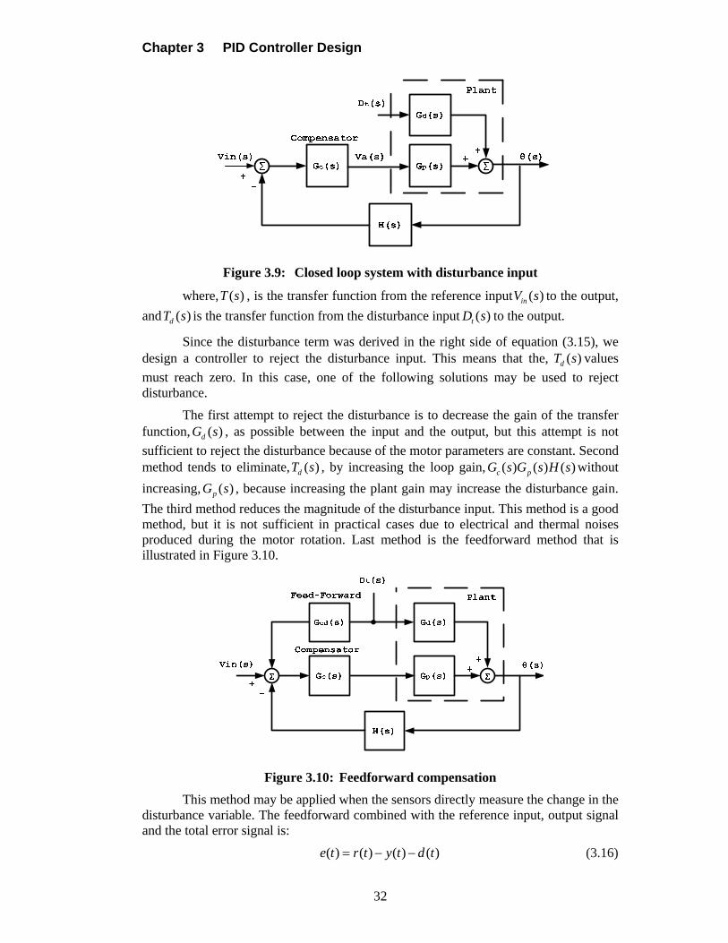
Chapter 3 PID Controller Design
32
Figure 3.9: Closed loop system with disturbance input
where, ( )T s , is the transfer function from the reference input ( )inV s to the output,
and ( )dT s is the transfer function from the disturbance input ( )tD s to the output.
Since the disturbance term was derived in the right side of equation (3.15), we design a controller to reject the disturbance input. This means that the, ( )dT s values
must reach zero. In this case, one of the following solutions may be used to reject disturbance.
The first attempt to reject the disturbance is to decrease the gain of the transfer function, ( )dG s , as possible between the input and the output, but this attempt is not
sufficient to reject the disturbance because of the motor parameters are constant. Second method tends to eliminate, ( )dT s , by increasing the loop gain, ( ) ( ) ( )c pG s G s H s without
increasing, ( )pG s , because increasing the plant gain may increase the disturbance gain.
The third method reduces the magnitude of the disturbance input. This method is a good method, but it is not sufficient in practical cases due to electrical and thermal noises produced during the motor rotation. Last method is the feedforward method that is illustrated in Figure 3.10.
Figure 3.10: Feedforward compensation
This method may be applied when the sensors directly measure the change in the disturbance variable. The feedforward combined with the reference input, output signal and the total error signal is:
( ) ( ) ( ) ( )e t r t y t d t (3.16)
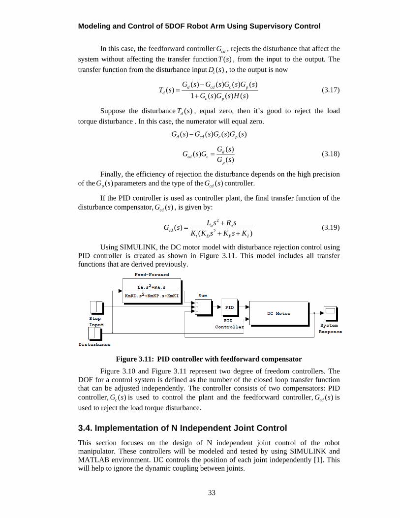
Modeling and Control of 5DOF Robot Arm Using Supervisory Control
33
In this case, the feedforward controller cdG , rejects the disturbance that affect the
system without affecting the transfer function ( )T s , from the input to the output. The
transfer function from the disturbance input ( )tD s , to the output is now
( ) ( ) ( ) ( )
( )1 ( ) ( ) ( )
d cd c pd
c p
G s G s G s G sT s
G s G s H s
(3.17)
Suppose the disturbance ( )dT s , equal zero, then it’s good to reject the load
torque disturbance . In this case, the numerator will equal zero.
( ) ( ) ( ) ( )d cd c pG s G s G s G s
( )
( )( )
dcd c
p
G sG s G
G s (3.18)
Finally, the efficiency of rejection the disturbance depends on the high precision of the ( )pG s parameters and the type of the ( )cdG s controller.
If the PID controller is used as controller plant, the final transfer function of the disturbance compensator, ( )cdG s , is given by:
2
2( )
( )a a
cdt D P I
L s R sG s
K K s K s K
(3.19)
Using SIMULINK, the DC motor model with disturbance rejection control using PID controller is created as shown in Figure 3.11. This model includes all transfer functions that are derived previously.
Figure 3.11: PID controller with feedforward compensator
Figure 3.10 and Figure 3.11 represent two degree of freedom controllers. The DOF for a control system is defined as the number of the closed loop transfer function that can be adjusted independently. The controller consists of two compensators: PID controller, ( )cG s is used to control the plant and the feedforward controller, ( )cdG s is
used to reject the load torque disturbance.
3.4. Implementation of N Independent Joint Control
This section focuses on the design of N independent joint control of the robot manipulator. These controllers will be modeled and tested by using SIMULINK and MATLAB environment. IJC controls the position of each joint independently [1]. This will help to ignore the dynamic coupling between joints.
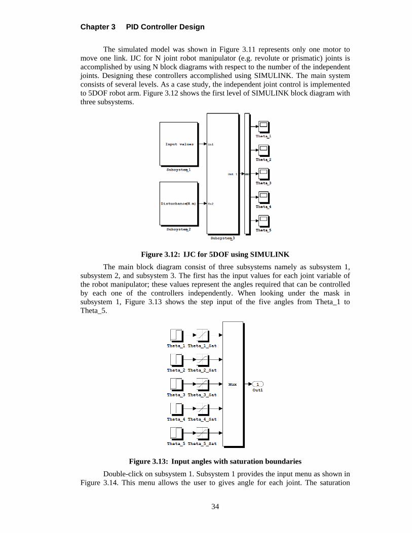
Chapter 3 PID Controller Design
34
The simulated model was shown in Figure 3.11 represents only one motor to move one link. IJC for N joint robot manipulator (e.g. revolute or prismatic) joints is accomplished by using N block diagrams with respect to the number of the independent joints. Designing these controllers accomplished using SIMULINK. The main system consists of several levels. As a case study, the independent joint control is implemented to 5DOF robot arm. Figure 3.12 shows the first level of SIMULINK block diagram with three subsystems.
Figure 3.12: IJC for 5DOF using SIMULINK
The main block diagram consist of three subsystems namely as subsystem 1, subsystem 2, and subsystem 3. The first has the input values for each joint variable of the robot manipulator; these values represent the angles required that can be controlled by each one of the controllers independently. When looking under the mask in subsystem 1, Figure 3.13 shows the step input of the five angles from Theta_1 to Theta_5.
Figure 3.13: Input angles with saturation boundaries
Double-click on subsystem 1. Subsystem 1 provides the input menu as shown in Figure 3.14. This menu allows the user to gives angle for each joint. The saturation
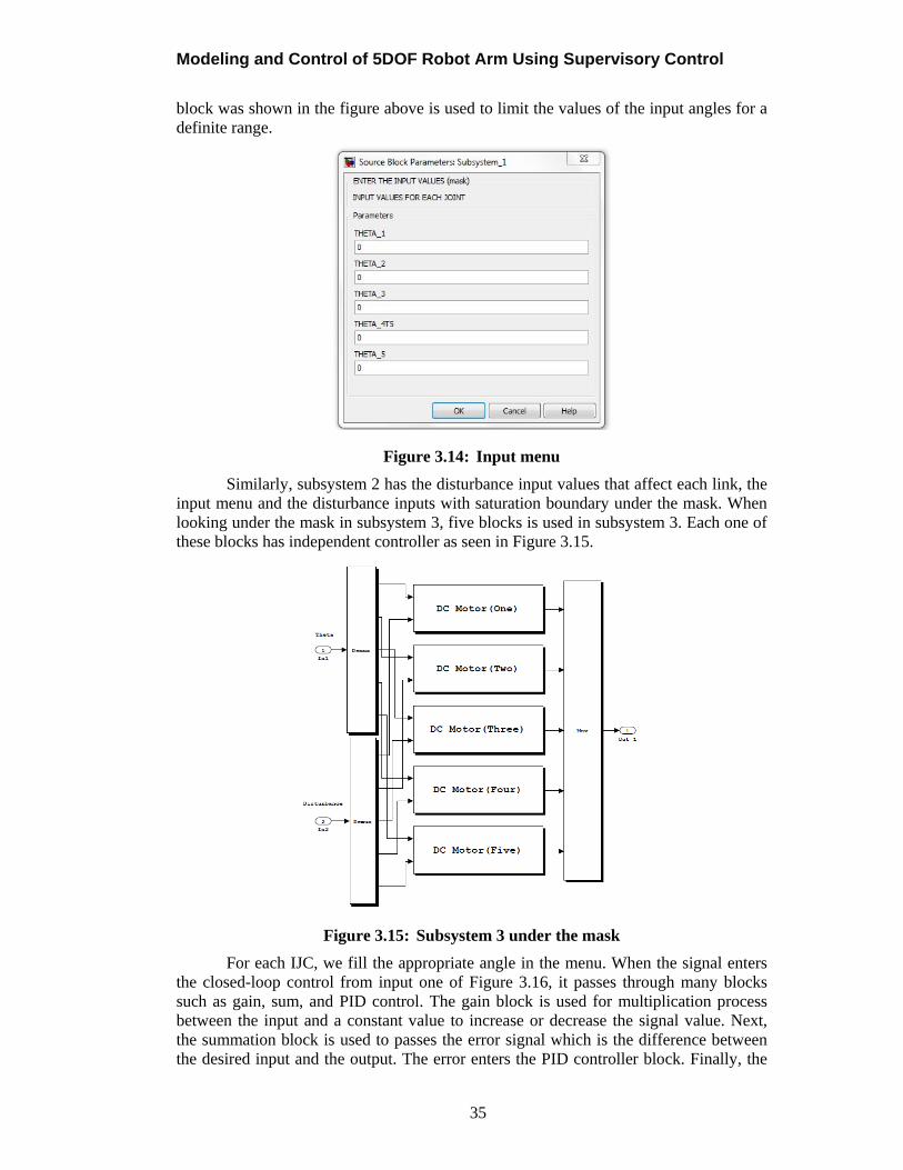
Modeling and Control of 5DOF Robot Arm Using Supervisory Control
35
block was shown in the figure above is used to limit the values of the input angles for a definite range.
Figure 3.14: Input menu
Similarly, subsystem 2 has the disturbance input values that affect each link, the input menu and the disturbance inputs with saturation boundary under the mask. When looking under the mask in subsystem 3, five blocks is used in subsystem 3. Each one of these blocks has independent controller as seen in Figure 3.15.
Figure 3.15: Subsystem 3 under the mask
For each IJC, we fill the appropriate angle in the menu. When the signal enters the closed-loop control from input one of Figure 3.16, it passes through many blocks such as gain, sum, and PID control. The gain block is used for multiplication process between the input and a constant value to increase or decrease the signal value. Next, the summation block is used to passes the error signal which is the difference between the desired input and the output. The error enters the PID controller block. Finally, the
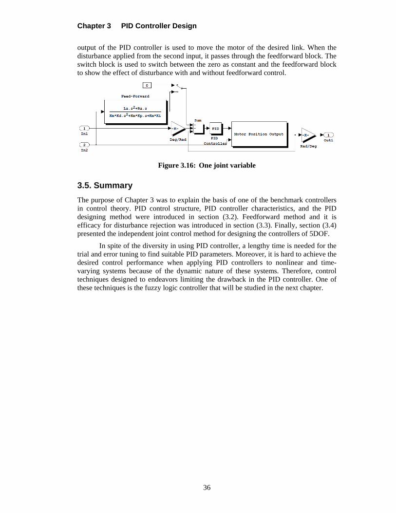
Chapter 3 PID Controller Design
36
output of the PID controller is used to move the motor of the desired link. When the disturbance applied from the second input, it passes through the feedforward block. The switch block is used to switch between the zero as constant and the feedforward block to show the effect of disturbance with and without feedforward control.
Figure 3.16: One joint variable
3.5. Summary
The purpose of Chapter 3 was to explain the basis of one of the benchmark controllers in control theory. PID control structure, PID controller characteristics, and the PID designing method were introduced in section (3.2). Feedforward method and it is efficacy for disturbance rejection was introduced in section (3.3). Finally, section (3.4) presented the independent joint control method for designing the controllers of 5DOF.
In spite of the diversity in using PID controller, a lengthy time is needed for the trial and error tuning to find suitable PID parameters. Moreover, it is hard to achieve the desired control performance when applying PID controllers to nonlinear and time-varying systems because of the dynamic nature of these systems. Therefore, control techniques designed to endeavors limiting the drawback in the PID controller. One of these techniques is the fuzzy logic controller that will be studied in the next chapter.
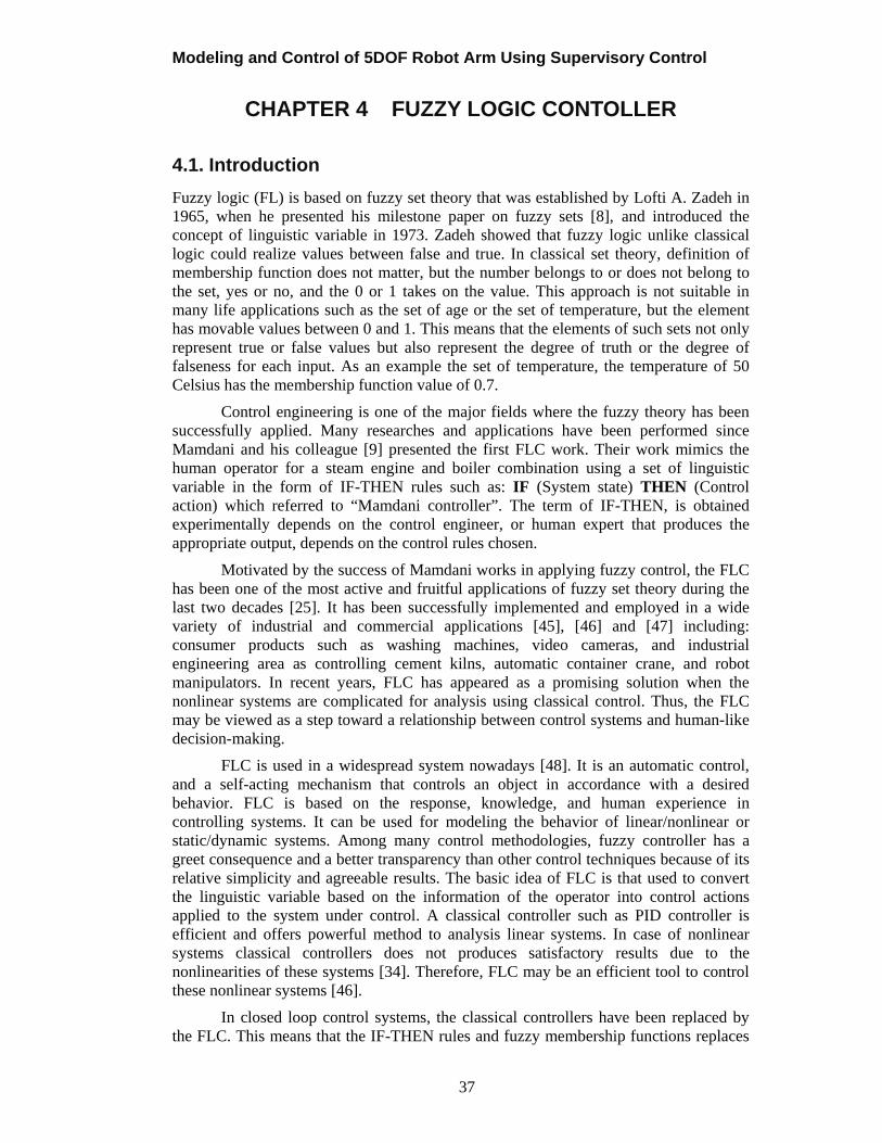
Modeling and Control of 5DOF Robot Arm Using Supervisory Control
37
CHAPTER 4 FUZZY LOGIC CONTOLLER
4.1. Introduction
Fuzzy logic (FL) is based on fuzzy set theory that was established by Lofti A. Zadeh in 1965, when he presented his milestone paper on fuzzy sets [8], and introduced the concept of linguistic variable in 1973. Zadeh showed that fuzzy logic unlike classical logic could realize values between false and true. In classical set theory, definition of membership function does not matter, but the number belongs to or does not belong to the set, yes or no, and the 0 or 1 takes on the value. This approach is not suitable in many life applications such as the set of age or the set of temperature, but the element has movable values between 0 and 1. This means that the elements of such sets not only represent true or false values but also represent the degree of truth or the degree of falseness for each input. As an example the set of temperature, the temperature of 50 Celsius has the membership function value of 0.7.
Control engineering is one of the major fields where the fuzzy theory has been successfully applied. Many researches and applications have been performed since Mamdani and his colleague [9] presented the first FLC work. Their work mimics the human operator for a steam engine and boiler combination using a set of linguistic variable in the form of IF-THEN rules such as: IF (System state) THEN (Control action) which referred to “Mamdani controller”. The term of IF-THEN, is obtained experimentally depends on the control engineer, or human expert that produces the appropriate output, depends on the control rules chosen.
Motivated by the success of Mamdani works in applying fuzzy control, the FLC has been one of the most active and fruitful applications of fuzzy set theory during the last two decades [25]. It has been successfully implemented and employed in a wide variety of industrial and commercial applications [45], [46] and [47] including: consumer products such as washing machines, video cameras, and industrial engineering area as controlling cement kilns, automatic container crane, and robot manipulators. In recent years, FLC has appeared as a promising solution when the nonlinear systems are complicated for analysis using classical control. Thus, the FLC may be viewed as a step toward a relationship between control systems and human-like decision-making.
FLC is used in a widespread system nowadays [48]. It is an automatic control, and a self-acting mechanism that controls an object in accordance with a desired behavior. FLC is based on the response, knowledge, and human experience in controlling systems. It can be used for modeling the behavior of linear/nonlinear or static/dynamic systems. Among many control methodologies, fuzzy controller has a greet consequence and a better transparency than other control techniques because of its relative simplicity and agreeable results. The basic idea of FLC is that used to convert the linguistic variable based on the information of the operator into control actions applied to the system under control. A classical controller such as PID controller is efficient and offers powerful method to analysis linear systems. In case of nonlinear systems classical controllers does not produces satisfactory results due to the nonlinearities of these systems [34]. Therefore, FLC may be an efficient tool to control these nonlinear systems [46].
In closed loop control systems, the classical controllers have been replaced by the FLC. This means that the IF-THEN rules and fuzzy membership functions replaces
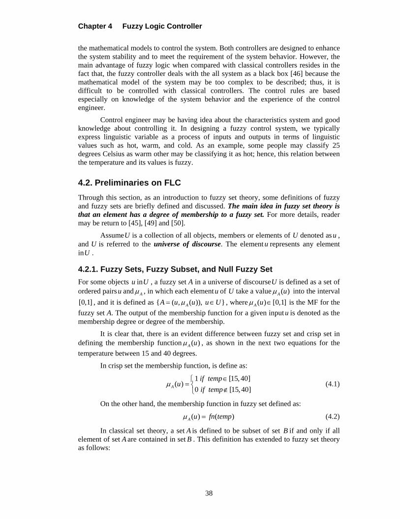
Chapter 4 Fuzzy Logic Controller
38
the mathematical models to control the system. Both controllers are designed to enhance the system stability and to meet the requirement of the system behavior. However, the main advantage of fuzzy logic when compared with classical controllers resides in the fact that, the fuzzy controller deals with the all system as a black box [46] because the mathematical model of the system may be too complex to be described; thus, it is difficult to be controlled with classical controllers. The control rules are based especially on knowledge of the system behavior and the experience of the control engineer.
Control engineer may be having idea about the characteristics system and good knowledge about controlling it. In designing a fuzzy control system, we typically express linguistic variable as a process of inputs and outputs in terms of linguistic values such as hot, warm, and cold. As an example, some people may classify 25 degrees Celsius as warm other may be classifying it as hot; hence, this relation between the temperature and its values is fuzzy.
4.2. Preliminaries on FLC
Through this section, as an introduction to fuzzy set theory, some definitions of fuzzy and fuzzy sets are briefly defined and discussed. The main idea in fuzzy set theory is that an element has a degree of membership to a fuzzy set. For more details, reader may be return to [45], [49] and [50].
AssumeU is a collection of all objects, members or elements of U denoted as u , and U is referred to the universe of discourse. The element u represents any element inU .
4.2.1. Fuzzy Sets, Fuzzy Subset, and Null Fuzzy Set
For some objects u inU , a fuzzy set A in a universe of discourseU is defined as a set of ordered pairsu and A , in which each elementu of U take a value ( )A u into the interval
[0,1] , and it is defined as { ( , ( )), }AA u u u U , where ( ) [0,1]A u is the MF for the
fuzzy set A. The output of the membership function for a given input u is denoted as the membership degree or degree of the membership.
It is clear that, there is an evident difference between fuzzy set and crisp set in defining the membership function ( )A u , as shown in the next two equations for the
temperature between 15 and 40 degrees.
In crisp set the membership function, is define as:
1 [15, 40]
( )0 [15,40]A
if tempu
if temp
(4.1)
On the other hand, the membership function in fuzzy set defined as:
( ) ( )A u fn temp (4.2)
In classical set theory, a set A is defined to be subset of set B if and only if all element of set A are contained in set B . This definition has extended to fuzzy set theory as follows:
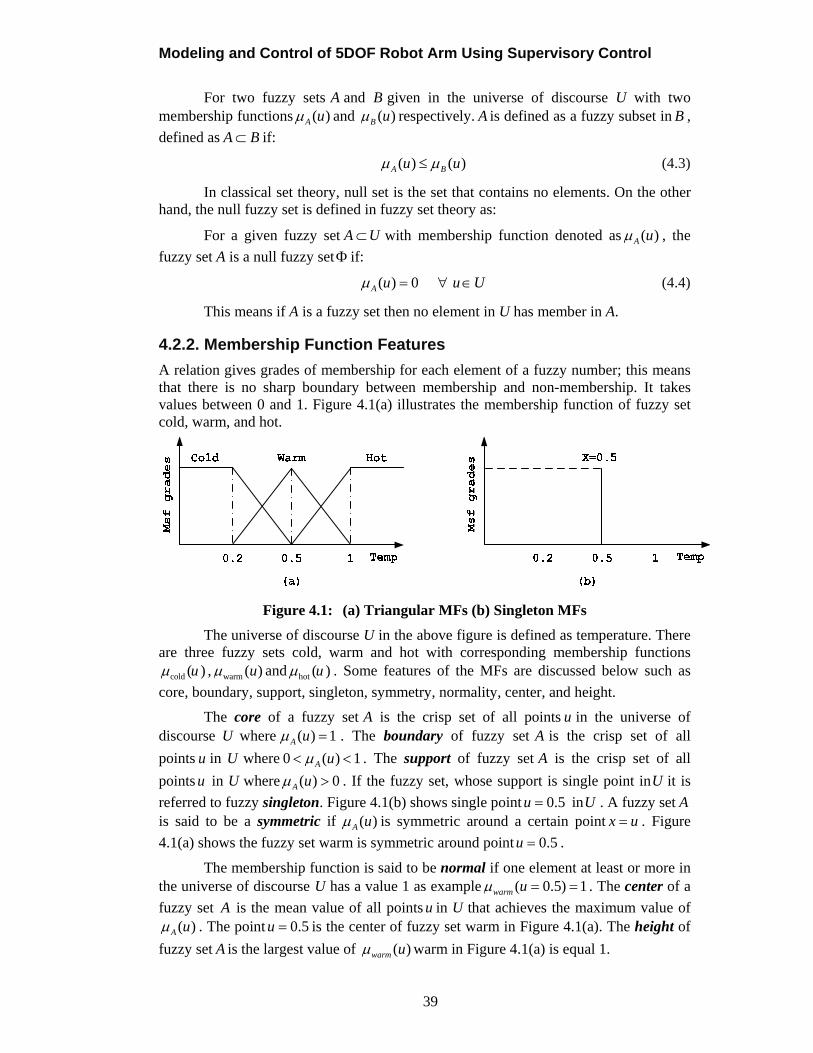
Modeling and Control of 5DOF Robot Arm Using Supervisory Control
39
For two fuzzy sets A and B given in the universe of discourse U with two membership functions ( )A u and ( )B u respectively. A is defined as a fuzzy subset in B ,
defined as A B if:
( ) ( )A Bu u (4.3)
In classical set theory, null set is the set that contains no elements. On the other hand, the null fuzzy set is defined in fuzzy set theory as:
For a given fuzzy set A U with membership function denoted as ( )A u , the
fuzzy set A is a null fuzzy set if:
( ) 0 A u u U (4.4)
This means if A is a fuzzy set then no element in U has member in A.
4.2.2. Membership Function Features
A relation gives grades of membership for each element of a fuzzy number; this means that there is no sharp boundary between membership and non-membership. It takes values between 0 and 1. Figure 4.1(a) illustrates the membership function of fuzzy set cold, warm, and hot.
Figure 4.1: (a) Triangular MFs (b) Singleton MFs
The universe of discourse U in the above figure is defined as temperature. There are three fuzzy sets cold, warm and hot with corresponding membership functions
cold ( )u , warm ( )u and hot ( )u . Some features of the MFs are discussed below such as
core, boundary, support, singleton, symmetry, normality, center, and height.
The core of a fuzzy set A is the crisp set of all points u in the universe of discourse U where ( ) 1A u . The boundary of fuzzy set A is the crisp set of all
points u in U where 0 ( ) 1A u . The support of fuzzy set A is the crisp set of all
points u in U where ( ) 0A u . If the fuzzy set, whose support is single point inU it is
referred to fuzzy singleton. Figure 4.1(b) shows single point 0.5u inU . A fuzzy set A is said to be a symmetric if ( )A u is symmetric around a certain point x u . Figure
4.1(a) shows the fuzzy set warm is symmetric around point 0.5u .
The membership function is said to be normal if one element at least or more in the universe of discourse U has a value 1 as example ( 0.5) 1warm u . The center of a
fuzzy set A is the mean value of all points u in U that achieves the maximum value of ( )A u . The point 0.5u is the center of fuzzy set warm in Figure 4.1(a). The height of
fuzzy set A is the largest value of ( )warm u warm in Figure 4.1(a) is equal 1.
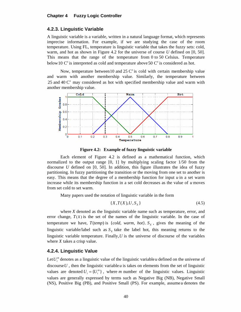
Chapter 4 Fuzzy Logic Controller
40
4.2.3. Linguistic Variable
A linguistic variable is a variable, written in a natural language format, which represents imprecise information. For example, if we are studying the case of the room temperature. Using FL, temperature is linguistic variable that takes the fuzzy sets: cold, warm, and hot as shown in Figure 4.2 for the universe of course U defined on [0, 50]. This means that the range of the temperature from 0 to 50 Celsius. Temperature below o10 C is interpreted as cold and temperature above o50 C is considered as hot.
Now, temperature between o10 and 25 C is cold with certain membership value and warm with another membership value. Similarly, the temperature between
o25 and 40 C may considered as hot with specified membership value and warm with another membership value.
Figure 4.2: Example of fuzzy linguistic variable
Each element of Figure 4.2 is defined as a mathematical function, which normalized to the output range [0, 1] by multiplying scaling factor 1/50 from the discourse U defined on [0, 50]. In addition, this figure illustrates the idea of fuzzy partitioning. In fuzzy partitioning the transition or the moving from one set to another is easy. This means that the degree of a membership function for input u in a set warm increase while its membership function in a set cold decreases as the value of u moves from set cold to set warm.
Many papers used the notation of linguistic variable in the form
{ , ( ), , }XX T X U S (4.5)
where X denoted as the linguistic variable name such as temperature, error, and error change, ( )XT is the set of the names of the linguistic variable. In the case of
temperature we have, ( )T temp is {cold, warm, hot}. XS , gives the meaning of the
linguistic variable/label such as XS take the label hot, this meaning returns to the
linguistic variable temperature. Finally,U is the universe of discourse of the variables where X takes a crisp value.
4.2.4. Linguistic Value
Let miU denotes as a linguistic value of the linguistic variableu defined on the universe of
discourseU , then the linguistic variable u is takes on elements from the set of linguistic values are denoted { }m
i iU U , where m number of the linguistic values. Linguistic
values are generally expressed by terms such as Negative Big (NB), Negative Small (NS), Positive Big (PB), and Positive Small (PS). For example, assume u denotes the

Modeling and Control of 5DOF Robot Arm Using Supervisory Control
41
linguistic variable temperature, then the linguistic values of the temperature variables are 1 ,iU cold 2 ,iU warm and 3
iU hot , so that miu U where 1 2 3
1 1 1 1{ , , }mU U U U .
4.2.5. Fuzzy Conditional Statement
For two inputs e and e and output u with a universe of discourses ,E E and U respectively. The fuzzy conditional statement consists of two parts: antecedent that represents the condition in the application domain and the consequent represents the control action for the controlled system. The IF-THEN fuzzy control rule has the form:
1 1 1 1
2 2 2 2
:
:
: j j j j
R e is A e is B u is C
R e is A e is B u is C
R e is A e is B u is C
IF AND THEN
IF AND THEN
IF AND THEN
.
where ,e e and u are linguistic variable representing two process state and one control variable. ,A B and C are linguistic values of the linguistic variables , e e and u in the universe of discourse ,E E andU respectively and 1, 2, ,j n .
4.2.6. Operations on Fuzzy Sets
The following operations are suggested by Zadeh to establish the concept of the fuzzy set theory. Assuming A and B are two fuzzy sets inU with MFs A and B respectively.
Fuzzy mathematics denoted as relation between the elements of A and B described using 1 2( , )A B u u , where 1 2, ,u u A B . The commonly used set operations are union,
intersection, and complement. The union of A and B means that all elements belong to A or B . The intersection of A and B is mean that, the collection of all elements belong to A and B. The complement of A is the elements, which do not belong to A. Figure 4.3, Figure 4.4, and Figure 4.5 shows the basic operation of the fuzzy set respectively.
1. Union
The union of two fuzzy sets A and B on the universe of discourse U is a fuzzy set C is described in the relation C A B , and the membership function of the fuzzy set C is described as following:
( ) ( ) max{ ( ), ( )}C A B A Bu u u u (4.6)
Moreover, it shown as:
( ) ( ) ( )C A Bu u u (4.7)
Figure 4.3: Union of fuzzy set A and B
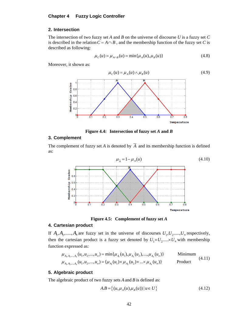
Chapter 4 Fuzzy Logic Controller
42
2. Intersection
The intersection of two fuzzy set A and B on the universe of discourse U is a fuzzy set C is described in the relationC A B , and the membership function of the fuzzy set C is described as following:
( ) ( ) min{ ( ), ( )}C A B A Bu u u u (4.8)
Moreover, it shown as:
( ) ( ) ( )C A Bu u u (4.9)
Figure 4.4: Intersection of fuzzy set A and B
3. Complement
The complement of fuzzy set A is denoted by A and its membership function is defined as:
1 ( )AAu (4.10)
Figure 4.5: Complement of fuzzy set A
4. Cartesian product
If 1 2, ,....., nA A A are fuzzy set in the universe of discourses 1 2, ....., nU U U respectively,
then the cartesian product is a fuzzy set denoted by 1 2..... nU U U with membership
function expressed as:
1 2 1 2
1 2 1 2
, ,..., 1 2 1 2
, ,..., 1 2 1 2
( , ,..., ) min{ ( ), ( ),..., ( )} Minimum
( , ,..., ) { ( ) ( ) ... ( )} Productn n
n n
n A A A n
n A A A n
A A A
A A A
u u u u u u
u u u u u u
(4.11)
5. Algebraic product
The algebraic product of two fuzzy sets A and B is defined as:
. ( , ( ). ( )) |A BA B u u u u U (4.12)
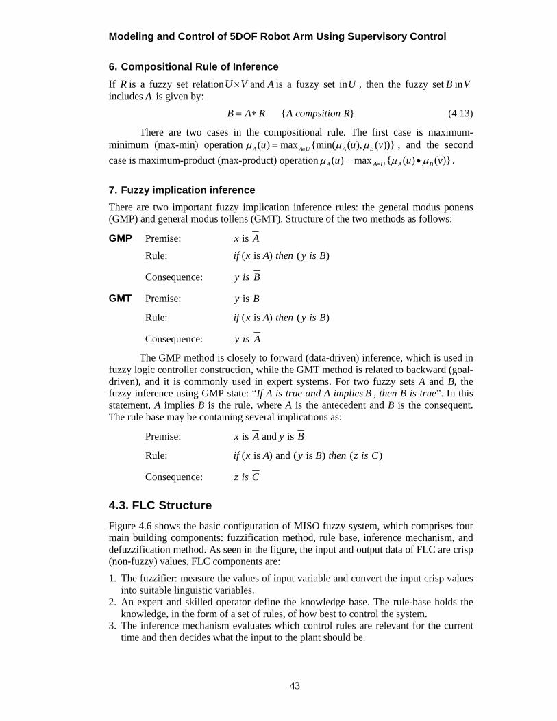
Modeling and Control of 5DOF Robot Arm Using Supervisory Control
43
6. Compositional Rule of Inference
If R is a fuzzy set relationU V and A is a fuzzy set inU , then the fuzzy set B inV includes A is given by:
{ }B A R A compsition R (4.13)
There are two cases in the compositional rule. The first case is maximum-minimum (max-min) operation ( ) max {min( ( ), ( ))}A A U A Bu u v , and the second
case is maximum-product (max-product) operation ( ) max { ( ) ( )}A A BA Uu u v .
7. Fuzzy implication inference
There are two important fuzzy implication inference rules: the general modus ponens (GMP) and general modus tollens (GMT). Structure of the two methods as follows:
GMP Premise: is x A
Rule: ( is ) ( )if x A then y is B
Consequence: y is B
GMT Premise: is y B
Rule: ( is ) ( )if x A then y is B
Consequence: y is A
The GMP method is closely to forward (data-driven) inference, which is used in fuzzy logic controller construction, while the GMT method is related to backward (goal-driven), and it is commonly used in expert systems. For two fuzzy sets A and B, the fuzzy inference using GMP state: “If A is true and A implies B , then B is true”. In this statement, A implies B is the rule, where A is the antecedent and B is the consequent. The rule base may be containing several implications as:
Premise: is and is x A y B
Rule: ( is ) and ( is ) ( )if x A y B then z is C
Consequence: z is C
4.3. FLC Structure
Figure 4.6 shows the basic configuration of MISO fuzzy system, which comprises four main building components: fuzzification method, rule base, inference mechanism, and defuzzification method. As seen in the figure, the input and output data of FLC are crisp (non-fuzzy) values. FLC components are:
1. The fuzzifier: measure the values of input variable and convert the input crisp values into suitable linguistic variables.
2. An expert and skilled operator define the knowledge base. The rule-base holds the knowledge, in the form of a set of rules, of how best to control the system.
3. The inference mechanism evaluates which control rules are relevant for the current time and then decides what the input to the plant should be.

Chapter 4 Fuzzy Logic Controller
44
4. The defuzzifier is the opposite operator of fuzzifier interface; it converts the conclusions reached by an inference mechanism into a real value as inputs to plant.
Figure 4.6: Fuzzy control system structure
Before illustrating FLC components, it is important to define the FLC inputs and output variables. As mentioned in Chapter 1, the controller is used to correct the error signal then supply appropriate input to the plant. Two inputs are used for FLC: the error that generated from the feedback loop and derivative of the error, or it may also have an integral input for fuzzy like PI controller. In addition, when designing a fuzzy like PID controller the three inputs are used, and the output is a control signal feeds the plant.
The three variables , e e and u of the FLC are the error, error change, and the
output action, and the variables , , e e u are their fuzzy counterparts respectively, y is
the output, and r is the set point, ek is the scale factor of the error input, dek is the scale
factor of the error derivative, and the uk is the output gain.
4.3.1. Fuzzification
Fuzzification is the first block inside the controller, which scale the input crisp value into a normalized universe of discourseU , then converts each crisp input data e and e to a degree of membership function ( )A u . In other word, the purpose of fuzzifier is to
transform the crisp input to fuzzy set defined in U and characterized by membership function ( ) : [0,1]A u U . The input and output memberships overlaps, and they are
scaled with respect to input-output of the fuzzy control. It is labeled by linguistic terms such as short, medium, and tall. For example, if the integer value 40 is the input, the fuzzification process converts the integer value into a linguistic variable.
The number of the linguistic variables for the input output domains specified by the designer. In addition, they should be as small as possible because the larger number of linguistic variables, the more complicated inference mechanism. The domain of the input variables e and e are chosen from the specification of the controlled system, similarly the domain of the output variable (control signal) u is chosen according to the desired output. Each of the two inputs and output are covered by seven fuzzy set variables: NB, NM, NS, ZE, PS, PM, and PB. Figure 4.7 shows several types of membership functions [51], such as a triangular, trapezoidal, Gaussian, singleton, and
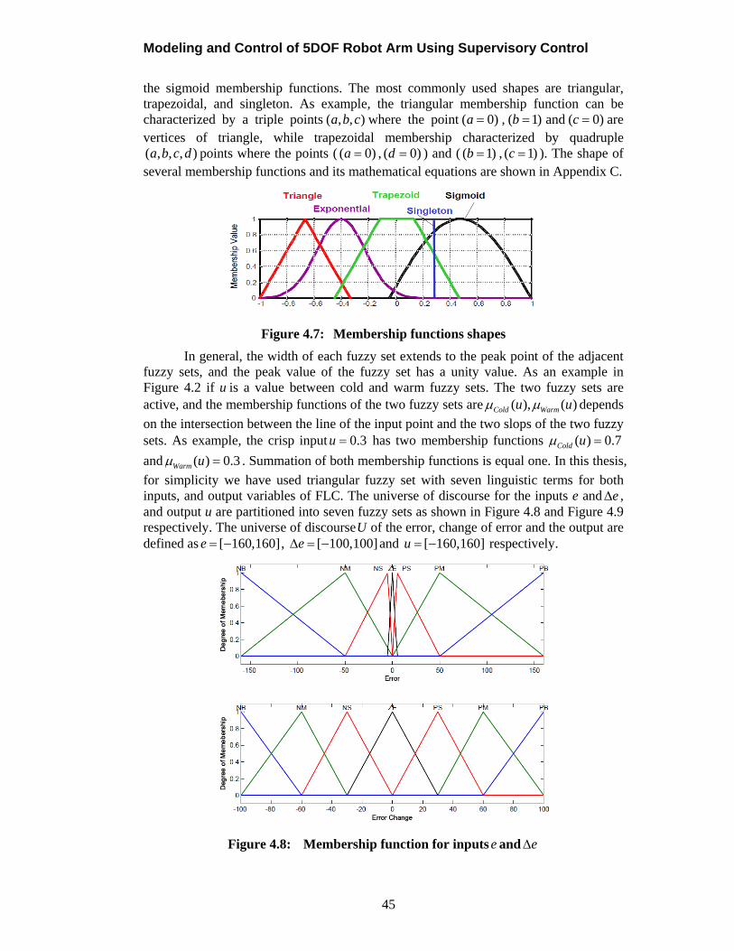
Modeling and Control of 5DOF Robot Arm Using Supervisory Control
45
the sigmoid membership functions. The most commonly used shapes are triangular, trapezoidal, and singleton. As example, the triangular membership function can be characterized by a triple points ( , , )a b c where the point ( 0)a , ( 1)b and ( 0)c are vertices of triangle, while trapezoidal membership characterized by quadruple ( , , , )a b c d points where the points ( ( 0)a , ( 0)d ) and ( ( 1)b , ( 1)c ). The shape of several membership functions and its mathematical equations are shown in Appendix C.
Figure 4.7: Membership functions shapes
In general, the width of each fuzzy set extends to the peak point of the adjacent fuzzy sets, and the peak value of the fuzzy set has a unity value. As an example in Figure 4.2 if u is a value between cold and warm fuzzy sets. The two fuzzy sets are active, and the membership functions of the two fuzzy sets are ( ), ( )Cold Warmu u depends
on the intersection between the line of the input point and the two slops of the two fuzzy sets. As example, the crisp input 0.3 u has two membership functions ( ) 0.7Cold u
and ( ) 0.3Warm u . Summation of both membership functions is equal one. In this thesis,
for simplicity we have used triangular fuzzy set with seven linguistic terms for both inputs, and output variables of FLC. The universe of discourse for the inputs e and e , and output u are partitioned into seven fuzzy sets as shown in Figure 4.8 and Figure 4.9 respectively. The universe of discourseU of the error, change of error and the output are defined as [ 160,160]e , [ 100,100]e and [ 160,160]u respectively.
Figure 4.8: Membership function for inputs e and e
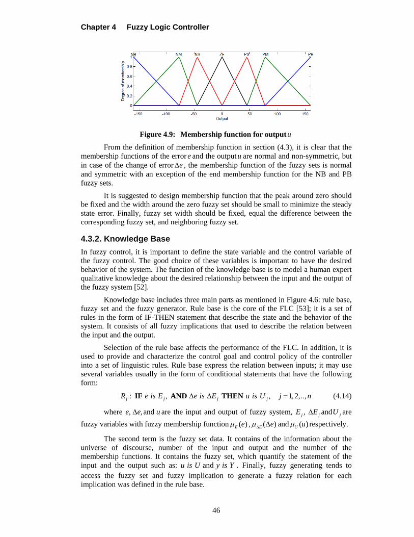
Chapter 4 Fuzzy Logic Controller
46
Figure 4.9: Membership function for outputu
From the definition of membership function in section (4.3), it is clear that the membership functions of the error e and the outputu are normal and non-symmetric, but in case of the change of error e , the membership function of the fuzzy sets is normal and symmetric with an exception of the end membership function for the NB and PB fuzzy sets.
It is suggested to design membership function that the peak around zero should be fixed and the width around the zero fuzzy set should be small to minimize the steady state error. Finally, fuzzy set width should be fixed, equal the difference between the corresponding fuzzy set, and neighboring fuzzy set.
4.3.2. Knowledge Base
In fuzzy control, it is important to define the state variable and the control variable of the fuzzy control. The good choice of these variables is important to have the desired behavior of the system. The function of the knowledge base is to model a human expert qualitative knowledge about the desired relationship between the input and the output of the fuzzy system [52].
Knowledge base includes three main parts as mentioned in Figure 4.6: rule base, fuzzy set and the fuzzy generator. Rule base is the core of the FLC [53]; it is a set of rules in the form of IF-THEN statement that describe the state and the behavior of the system. It consists of all fuzzy implications that used to describe the relation between the input and the output.
Selection of the rule base affects the performance of the FLC. In addition, it is used to provide and characterize the control goal and control policy of the controller into a set of linguistic rules. Rule base express the relation between inputs; it may use several variables usually in the form of conditional statements that have the following form:
: , , 1, 2,..,j j j jR e is E e is E u is U j n IF AND THEN (4.14)
where , , and e e u are the input and output of fuzzy system, , j jE E and jU are
fuzzy variables with fuzzy membership function ( )E e , ( )E e and ( )U u respectively.
The second term is the fuzzy set data. It contains of the information about the universe of discourse, number of the input and output and the number of the membership functions. It contains the fuzzy set, which quantify the statement of the input and the output such as: u is U and y is Y . Finally, fuzzy generating tends to access the fuzzy set and fuzzy implication to generate a fuzzy relation for each implication was defined in the rule base.
Modeling and Control of 5DOF Robot Arm Using Supervisory Control
47
Many categories was proposed to form the IF-THEN statement. Two prevalent methods are Mamdani and Takagi-Sugeno [54]. The first method, is considered as the most popular method is used to design FLC because it is simple to be implemented. The second is Takage-Sugeno (TS) method, which is called TS fuzzy rule. The two methods have a fuzzy antecedent part. The antecedent evaluation of the IF-THEN statement is the same for both methods, but the essential difference between them lies in the consequent part structure, where the consequent part of TS rule is a function of real value. The next two rules structure describes Mamdani and TS fuzzy methods.
Mamdani style
is / is is i i j j ij ije E e E u U IF AND OR THEN (4.15)
Sugeno style
is / is i i j j ij i i j je E e E u k u k u IF AND OR THEN (4.16)
In Mamdani fuzzy rule method, the knowledge of the system (antecedent) and the set of the action (consequent) depend on the human operator. Through the thesis, Mamdani fuzzy rule is adopted to construct the fuzzy model of the system, which is a robot manipulator with SISO. This method was structured with two inputs as antecedent and one output as the consequence with variables (e, e , u and R) as error, error change, output, and rules respectively.
Generally, for nonlinear systems the linguistic rule is one of four forms. Each one of these forms expressed linguistically as:
Single Input single output (SISO)
e is E u is UIF THEN (4.17)
Multi input single output (MISO)
1 1 2 2 e is E e is E u is UIF AND THEN (4.18)
Single Input multi output (SIMO)
1 1 1 1 2 2 e is E u is U u is UIF THEN AND (4.19)
Multi input multi output (MIMO)
1 1 1 1 ... ... r r r re is E e is E u is U u is UIF AND AND THEN AND AND (4.20)
In this thesis, the rule base is constructed as referred in the second and fourth cases. These cases will use in Chapter 4 and Chapter 5 respectively.
There are some techniques are used for generating rule base. These techniques may combine to construct an effective method to derive rule base [45] and [47]. Derivation rule base depends on using the antecedent (error and error change) and the consequent (control signal) to describe the relation between the inputs and outputs of the fuzzy controller. First technique is based on the knowledge of the controlled system by analyzing the behavior of the system. We can use the input output relation that obtained from system identification to generate a set of fuzzy rules to achieve the optimal behavior of the system. Although this method does not effective for all systems due to complexity and nonlinearity, it gives good results.
The second method is based on experienced human operator [52]. In many industrial control systems, the relation between the inputs and the output are not known
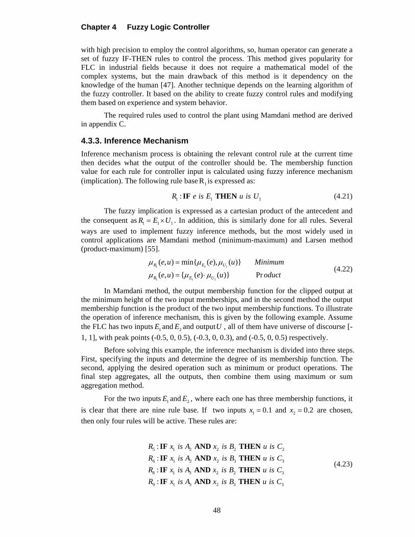
Chapter 4 Fuzzy Logic Controller
48
with high precision to employ the control algorithms, so, human operator can generate a set of fuzzy IF-THEN rules to control the process. This method gives popularity for FLC in industrial fields because it does not require a mathematical model of the complex systems, but the main drawback of this method is it dependency on the knowledge of the human [47]. Another technique depends on the learning algorithm of the fuzzy controller. It based on the ability to create fuzzy control rules and modifying them based on experience and system behavior.
The required rules used to control the plant using Mamdani method are derived in appendix C.
4.3.3. Inference Mechanism
Inference mechanism process is obtaining the relevant control rule at the current time then decides what the output of the controller should be. The membership function value for each rule for controller input is calculated using fuzzy inference mechanism (implication). The following rule base 1R is expressed as:
1 1 1: R e is E u is UIF THEN (4.21)
The fuzzy implication is expressed as a cartesian product of the antecedent and the consequent as 1 1 1R E U . In addition, this is similarly done for all rules. Several
ways are used to implement fuzzy inference methods, but the most widely used in control applications are Mamdani method (minimum-maximum) and Larsen method (product-maximum) [55].
1 1 1
1 1 1
( , ) min{ ( ), ( )}
( , ) { ( ) ( )} Pr
R E U
R E U
e u e u Minimum
e u e u oduct
(4.22)
In Mamdani method, the output membership function for the clipped output at the minimum height of the two input memberships, and in the second method the output membership function is the product of the two input membership functions. To illustrate the operation of inference mechanism, this is given by the following example. Assume the FLC has two inputs 1E and 2E and outputU , all of them have universe of discourse [-
1, 1], with peak points (-0.5, 0, 0.5), (-0.3, 0, 0.3), and (-0.5, 0, 0.5) respectively.
Before solving this example, the inference mechanism is divided into three steps. First, specifying the inputs and determine the degree of its membership function. The second, applying the desired operation such as minimum or product operations. The final step aggregates, all the outputs, then combine them using maximum or sum aggregation method.
For the two inputs 1E and 2E , where each one has three membership functions, it
is clear that there are nine rule base. If two inputs 1 0.1 x and 2 0.2 x are chosen,
then only four rules will be active. These rules are:
5 1 2 2 2 2
6 1 2 2 3 3
8 1 3 2 2 3
9 1 3 2 3 3
:
:
:
:
R x is A x is B u is C
R x is A x is B u is C
R x is A x is B u is C
R x is A x is B u is C
IF AND THEN
IF AND THEN
IF AND THEN
IF AND THEN
(4.23)
Modeling and Control of 5DOF Robot Arm Using Supervisory Control
49
Figure 4.10: Inference process using Mamdani and Larson methods
From Figure 4.10, the values of the membership functions of the proposed fuzzy sets are: 2 1( ) 0.8A x , 3 1( ) 0.2A x , 2 2( ) 0.18B x and 3 2( ) 0.82B x . Two inference
methods are used to calculate the weight of the four rules: first, Mamdani method. The weight of the rules is 1 2 1 2 2min( ( ), ( )) min(0.8,0.18) 0.18A Bw x x . Similarly,
3 0.18w and 4 0.2w . Weight of the rules solved using Larson inference mechanism
is 1 2 1 2 2( ). ( ) 0.144A Bw x x , similarly 2 0.656,w 3 0.036w and 4 0.164w . The
control action of both rules will be determined using a centroid of area defuzzification method in the next section.
In this example, the inference mechanism is called First Inference Then Aggregation (FITA), since the output of each rule is inferred first using composition rule of inference in each rule of the rule set, and the overall output is obtained using the max operation. Simulation test is carried out with the Fuzzy Toolbox for MATLAB and SIMULINK.
4.3.4 Defuzzification
Defuzzification method is the final stage of the FLC. After the inference mechanism is finished. The defuzzification method tends converts the resulting fuzzy set into a crisp values that can be sent to the plant as a control signal.
In general, there are several methods used for defuzzification such as centroid of area (COA), maximum method (MM), mean of maximum (MOM), and bisector of area (BOA) [56]. The most frequently used are COA, MM, and MOM methods. First, MOM method produces the control action that represents the mean value of the all control actions whose membership function has the max value. Second is MM method that produces control action, which the fuzzy set reaches the maximum point. This method is divided into two parts: first, the smallest of max (SOM), which has the minimum value of the support of fuzzy set. The second method is the largest of max (LOM), which has the maximum value of the support of the fuzzy set.
The last is COA method that is used through this thesis. This method produces a control action that represents the center of the output of the fuzzy set. The weighted average of the membership function or the COA bounded by the membership function curve and it is converted to a typical crisp value. This method yield:
Chapter 4 Fuzzy Logic Controller
50
1
1
( ).
( )
m
i ii
m
ii
x xu
x
(4.24)
A graphical interpretation of defuzzification methods is presented in Appendix C. Figure 4.11 shows the various defuzzification methods.
Figure 4.11: Defuzzification methods
The control action for the values, which obtained using Mamdani and Larson methods through section (4.4.3) using COA method, is determined as follows.
Mamdani Method
Control action = 1
1
( ).
( )
m
i ii
m
ii
x x
x
=
0.18*0 0.8*0.5 0.18*0.5 0.2*0.50.4338
0.18 0.8 0.18 0.2
Larson Method
Control action = 0.144*0 0.656*0.5 0.036*0.5 0.164*0.5
0.4280.144 0.656 0.036 0.164
4.4. Fuzzy Control
Fuzzy PID controller has been applied successfully in many applications of control fields. Different design methods of fuzzy PID controller are used nowadays [10], [26] and [57] that present significant performance comparing to classical PID controller; moreover, designing and tuning fuzzy PID controller with simple structure gives satisfactory results for the system. Fuzzy PID controller is good controller because its components help to provide convenient closed loop response characteristics. It combines the advantages of each term of PID controller individually as mentioned in Chapter 3, taking into account that the fuzzy PID terms are better than the classical PID terms [46]. Fuzzy proportional term reduces the rising time, while the fuzzy integral term eliminates the steady state error, and the third fuzzy derivative term enhances the system stability by reducing the overshoot and improving the transient response.
Generally, the number of rules, which cover all possible inputs equal number of fuzzy sets of first input multiplied by the number of the fuzzy sets of the second input. As an example, a fuzzy controller with two inputs (error and change of error) each one has 7 fuzzy sets. The possible rules are 49 (7 7) rules that cover all possible input variation. Similarly if number of the inputs are (increased / decreased) the number of the

Modeling and Control of 5DOF Robot Arm Using Supervisory Control
51
rules will (increased/decreased) [28]. As mentioned above, there are several types of fuzzy PID controller discussed. Through this thesis, two categories of fuzzy PID controller will be discussed as follows:
1. Three inputs structure with and without coupled rules. 2. Two inputs structure with and without coupled rules.
In the first category, the similarities between the three input structure of fuzzy PID controller with and without coupled rules each have three inputs and one output. In the first structure, the three inputs fed the same fuzzy PID controller, but in the second. Each input feeds individual fuzzy controller.
Type I of the first category is three input structure with coupled rules. This type is difficult because the number of the rules increases as the number of the input variables increases. For example, if there are three inputs each one has N fuzzy sets, this means that the total number of the required rules for this structure is 1 2 3N N N . So
this operation becomes very tedious and complicated. This requires the computer to process a huge database, mathematical operation and longer computational time. Type I of fuzzy PID controller expressed as:
is is E is is PID PIDe E e e E u U IF AND AND THEN (4.25)
The final PID control output is produced after taking the cumulative sum of the FLC output as shown in Figure 4.12.
Figure 4.12: Three input fuzzy PID (Type I)
Type II is the three input structure without coupled (with decoupled) rules. Figure 4.13 shows structure of fuzzy PID controller of the three inputs with decoupled rules. In this structure, each one of the controller inputs has independent controller unlike type I. In addition, the control output is represented by a separated set of rules.
Figure 4.13: Three input fuzzy PID (Type II)
The rule base in this structure is represented as follows:
is is
is E is
is is
P P
D D
I I
e E u U
e u U
e E u U
IF THEN
IF THEN
IF THEN
(4.26)
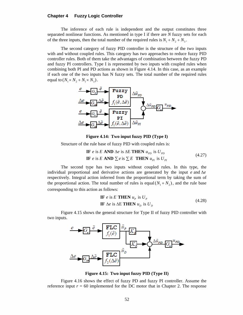
Chapter 4 Fuzzy Logic Controller
52
The inference of each rule is independent and the output constitutes three separated nonlinear functions. As mentioned in type I if there are N fuzzy sets for each of the three inputs, then the total number of the required rules is 1 2 3N N N .
The second category of fuzzy PID controller is the structure of the two inputs with and without coupled rules. This category has two approaches to reduce fuzzy PID controller rules. Both of them take the advantages of combination between the fuzzy PD and fuzzy PI controllers. Type I is represented by two inputs with coupled rules when combining both PI and PD actions as shown in Figure 4.14. In this case, as an example if each one of the two inputs has N fuzzy sets. The total number of the required rules equal to 1 2 1 3( )N N N N .
Figure 4.14: Two input fuzzy PID (Type I)
Structure of the rule base of fuzzy PID with coupled rules is:
is is E is
is is is PD PD
PI PI
e E e u U
e E e E u U
IF AND THEN
IF AND THEN (4.27)
The second type has two inputs without coupled rules. In this type, the individual proportional and derivative actions are generated by the input and e e respectively. Integral action inferred from the proportional term by taking the sum of the proportional action. The total number of rules is equal 1 2( )N N , and the rule base
corresponding to this action as follows:
is is
is E is P P
D D
e E u U
e u U IF THEN
IF THEN (4.28)
Figure 4.15 shows the general structure for Type II of fuzzy PID controller with two inputs.
Figure 4.15: Two input fuzzy PID (Type II)
Figure 4.16 shows the effect of fuzzy PD and fuzzy PI controller. Assume the reference input r = 60 implemented for the DC motor that in Chapter 2. The response
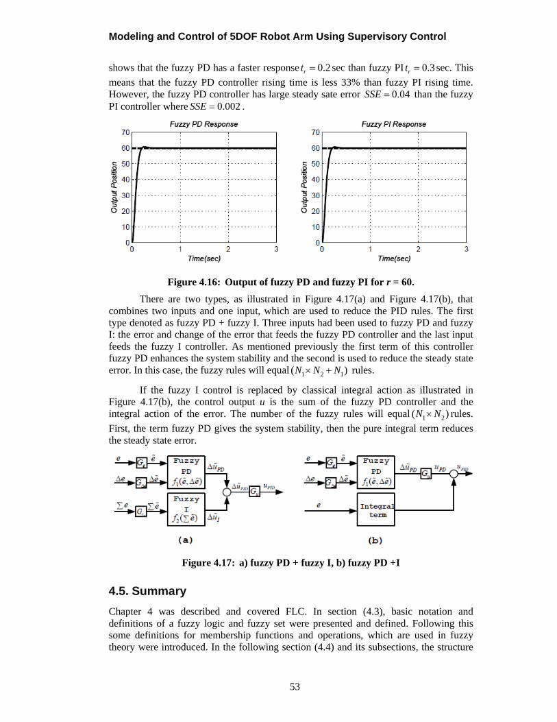
Modeling and Control of 5DOF Robot Arm Using Supervisory Control
53
shows that the fuzzy PD has a faster response 0.2rt sec than fuzzy PI 0.3rt sec. This
means that the fuzzy PD controller rising time is less 33% than fuzzy PI rising time. However, the fuzzy PD controller has large steady sate error 0.04SSE than the fuzzy PI controller where 0.002SSE .
Figure 4.16: Output of fuzzy PD and fuzzy PI for r = 60.
There are two types, as illustrated in Figure 4.17(a) and Figure 4.17(b), that combines two inputs and one input, which are used to reduce the PID rules. The first type denoted as fuzzy PD + fuzzy I. Three inputs had been used to fuzzy PD and fuzzy I: the error and change of the error that feeds the fuzzy PD controller and the last input feeds the fuzzy I controller. As mentioned previously the first term of this controller fuzzy PD enhances the system stability and the second is used to reduce the steady state error. In this case, the fuzzy rules will equal 1 2 1( )N N N rules.
If the fuzzy I control is replaced by classical integral action as illustrated in Figure 4.17(b), the control output u is the sum of the fuzzy PD controller and the integral action of the error. The number of the fuzzy rules will equal 1 2( )N N rules.
First, the term fuzzy PD gives the system stability, then the pure integral term reduces the steady state error.
Figure 4.17: a) fuzzy PD + fuzzy I, b) fuzzy PD +I
4.5. Summary
Chapter 4 was described and covered FLC. In section (4.3), basic notation and definitions of a fuzzy logic and fuzzy set were presented and defined. Following this some definitions for membership functions and operations, which are used in fuzzy theory were introduced. In the following section (4.4) and its subsections, the structure
Chapter 4 Fuzzy Logic Controller
54
of the FLC was presented. It consists of four components: fuzzifier, rule base, inference mechanism, and defuzzifier. Finally, section (4.5) was presented method for designing fuzzy controller and the effect of the number of the input and output variables on the derivation of the rule base.
This chapter is concluded by the following characteristics of the FLC in comparison to PID control techniques, which is used as reference benchmark for other techniques:
Fuzzy logic control deals with the system without requiring a lot of information about the dynamics of the system.
Fuzzy logic controller is nonlinear control and the design of FLC parameters depends on the characteristics of the system.
Fuzzy logic controller is more robust than a classical controller is, and it uses the linguistic data to find the suitable step response.
Modeling and Control of 5DOF Robot Arm Using Supervisory Control
55
CHAPTER 5 FUZZY SUPERVISORY CONTROLLER
5.1. Introduction
Although a large amount of literature discussed the FLC and PID control problem, the research in tuning PID parameters using supervisory control is still at an early stage.
In fuzzy theory, FLC grouped into two classes [57]: direct fuzzy controller (DFC) and indirect fuzzy controller (IFC). Through this thesis, the first type of fuzzy controller is used. DFC computes the controller action through the fuzzy mechanism, then the output control signal of the fuzzy controller feeds the plant. DFC is classified into three categories: First, the direct (pure) fuzzy controller, second FSC, and the third is a combination between both two categories [10]. In the first and the second type of direct fuzzy controller, the fuzzy reasoning attempts to provide a nonlinear action to control the output. Therefore, the fuzzy tuning PID controller is considered as nonlinear controller in contrast to linear PID controller in the conventional theory.
An adaptive controller is “a controller with adjustable parameters and a mechanism for adjusting parameters” [51]. A supervisory controller is a type of adaptive controllers since it searches to observe the current behavior of the plant and modifies the controlling unit “PID” to improve the performance. In other words, the design task of FSC has two main issues: first determine the knowledge parameter to generate the necessary crisp control action, then tune these parameters to obtain the desired performance for the plant. Fuzzy adaptive controller has two types: in first type, the rule base of the FLC is updated via a fuzzy system [58]. In the second type, the supervisory controller tends to monitors the controller when it does not properly tuned, then seeks to adjust the controller to obtain the desired response. The appreciation of fuzzy controller is easier to implement because it needs a little knowledge about the process, it reduces the difficulty of fine-tuning of the PID parameters and improves the response online during operation.
FLC is better than the PID controller when dealing with nonlinear systems. On the other hand, PID controller is used in more than 90% of control applications. Therefore, it is costly to replace the PID controller with FLC in all applications. Thus, one of the motivating and attractive solutions is to combine the PID controller and FLC to form the FSC. In real environments, unexpected changes in system characteristics may occurs, which causes the system to produce undesirable output. Therefore, the adaptive “supervisor” controller has the capabilities to change the PID parameters under varying process conditions. In other words, it should change the parameters of the control system to prevent the undesired behavior from occurring because the adaptive action is based upon the performance indices of the system.
5.2. Fuzzy Supervisory Controller Structure
This section is divided into three sections: first PID controller, second FLC and the third is FSC. As mentioned previously PID controller is considered as one of the most popular control technique used to control systems. Designing of the PID controller tends to tune PK , IK and DK parameters to observe how the system effect by these parameters.
Tuning PID parameters is classified into two methods: first, classical tuning and the second is tuning PID using supervisory controller [59]. PID parameters are fixed

Chapter 5 Fuzzy Supervisory Controller
56
during process control after they have been tuned for the first time. Since the fixed PID, parameters do not produce satisfactory results for systems. Therefore, this method is not a good choice in nonlinear circumstances. Therefore, the second method is used to overcome the limitation of tuning PID gains. This method depends on tuning these parameters on-line during process operation. This is accomplished using FLC, as supervisory for tuning PID parameters.
Some rules for tuning PID parameters are discussed as follows:
If the error ( ) ( ) ( )e t r t y t is positive large, then the proportional gain PK must be
large, integral term IK small and the derivative term DK is small. Therefore, this will
speed the system output.
If the current error is very small, the PID parameters will have to be a smaller value for proportional gain, larger value of integral time constant and larger value of derivative gain. Therefore, the speed of the system response will be small to reduce the overshoot of the output.
If the current error and its first difference are approaching zero (i.e. the system output will approach the steady state), then these parameters of PID controller must keep the values of the last state (i.e. the changes of these parameters must be very small). Therefore, this work will maintain the system output at the set point, and let the system output approach the steady state, etc....
Classical tuning methods are boring because a lot of time has to be spent to obtain the values of the three parameters. Therefore, FLC is a good choice for tuning PID gains online. Research in fuzzy controller design method is divided into two strategies: fuzzy control structure design and fuzzy control parameters design methods. First strategy intends to achieve the optimal control solution based on choice of the fuzzy controller structure such as number of inputs and outputs, fuzzification method, number and shape of membership function, defuzzification method, and rule base structure. Disadvantages of the first that the complexity of the fuzzy controller is increased as the number of the inputs increased. On the other side, the purpose of fuzzy controller parameter design is to find the optimal control solution by adjusting the parameters of the fuzzy controller with fixed structure. The parameter adjusting depends on the shape and the position of the membership function, and the scaling factor of the fuzzy controller.
The third controller is the FSC. Many papers [34], [35], [60], [61] and [62] discussed the FSC problem. FSC means that the fuzzy controller tunes PID parameters
PK , IK and DK . The constant PID parameters are not properly for nonlinear plants with
unpredictable variables. Hence, it is necessary to be tuned automatically. The basic structure of fuzzy supervisory PID controller is shown in Figure 5.1. This structure has the form of PID controller but its parameters are adopted using the FLC, which provides a rule base on the fuzzy inference. Fuzzy inference provides a rule base to change these parameters within initial parameters [62]. Regarding the supervisory structure, it consists of two levels. FLC that is represent the upper level and the PID controller as a lower level, which is tuned using FLC.
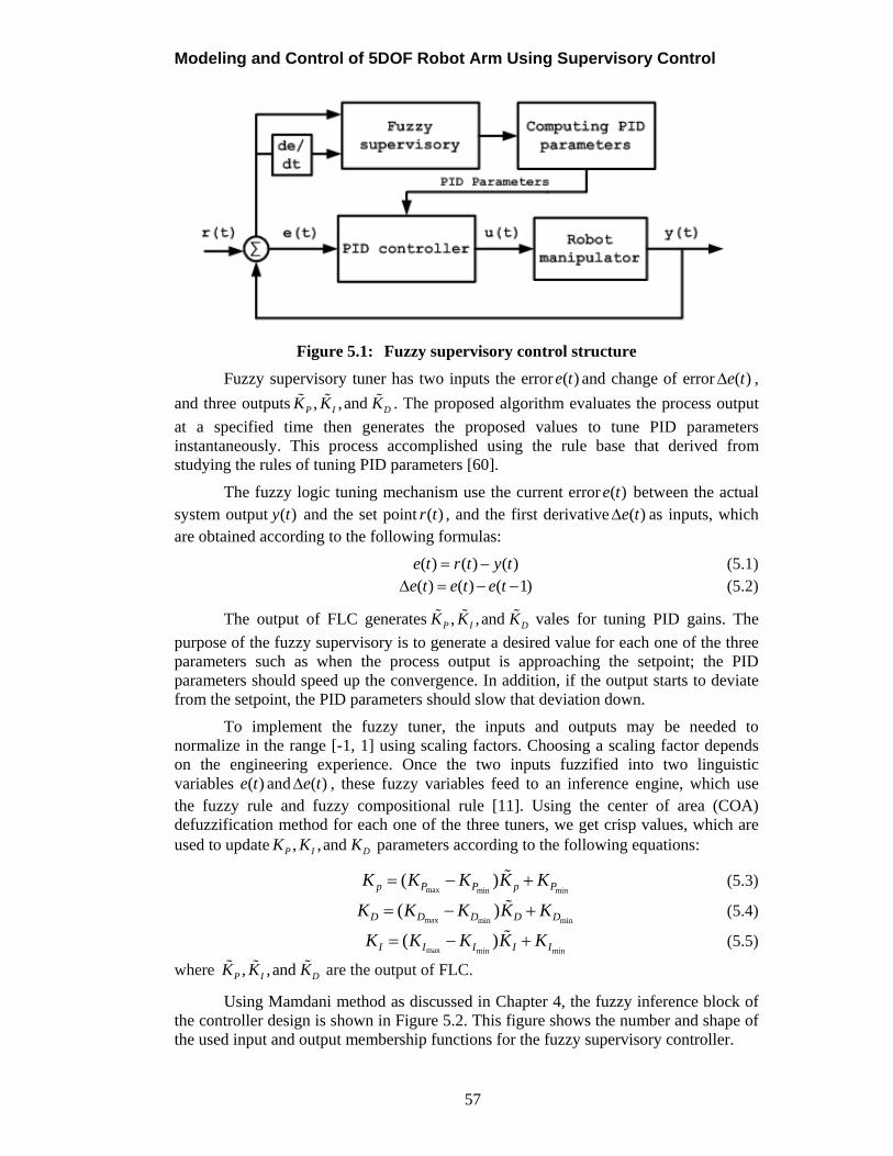
Modeling and Control of 5DOF Robot Arm Using Supervisory Control
57
Figure 5.1: Fuzzy supervisory control structure
Fuzzy supervisory tuner has two inputs the error ( )e t and change of error ( )e t ,
and three outputs , , and P I DK K K . The proposed algorithm evaluates the process output
at a specified time then generates the proposed values to tune PID parameters instantaneously. This process accomplished using the rule base that derived from studying the rules of tuning PID parameters [60].
The fuzzy logic tuning mechanism use the current error ( )e t between the actual system output ( )y t and the set point ( )r t , and the first derivative ( )e t as inputs, which are obtained according to the following formulas:
( ) ( ) ( )e t r t y t (5.1) ( ) ( ) ( 1)e t e t e t (5.2)
The output of FLC generates , , and P I DK K K vales for tuning PID gains. The
purpose of the fuzzy supervisory is to generate a desired value for each one of the three parameters such as when the process output is approaching the setpoint; the PID parameters should speed up the convergence. In addition, if the output starts to deviate from the setpoint, the PID parameters should slow that deviation down.
To implement the fuzzy tuner, the inputs and outputs may be needed to normalize in the range [-1, 1] using scaling factors. Choosing a scaling factor depends on the engineering experience. Once the two inputs fuzzified into two linguistic variables ( )e t and ( )e t , these fuzzy variables feed to an inference engine, which use the fuzzy rule and fuzzy compositional rule [11]. Using the center of area (COA) defuzzification method for each one of the three tuners, we get crisp values, which are used to update , , and P I DK K K parameters according to the following equations:
max min min
( )p pP P PK K K K K (5.3)
max min min
( )D D D D DK K K K K (5.4)
max min min
( )I I I I IK K K K K (5.5)
where , , and P I DK K K are the output of FLC.
Using Mamdani method as discussed in Chapter 4, the fuzzy inference block of the controller design is shown in Figure 5.2. This figure shows the number and shape of the used input and output membership functions for the fuzzy supervisory controller.
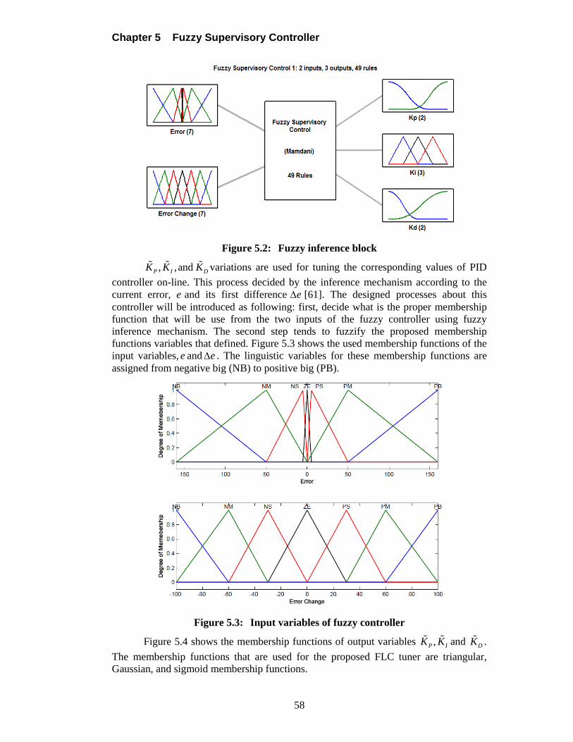
Chapter 5 Fuzzy Supervisory Controller
58
Figure 5.2: Fuzzy inference block
, , and P I DK K K variations are used for tuning the corresponding values of PID
controller on-line. This process decided by the inference mechanism according to the current error, e and its first difference e [61]. The designed processes about this controller will be introduced as following: first, decide what is the proper membership function that will be use from the two inputs of the fuzzy controller using fuzzy inference mechanism. The second step tends to fuzzify the proposed membership functions variables that defined. Figure 5.3 shows the used membership functions of the input variables, e and e . The linguistic variables for these membership functions are assigned from negative big (NB) to positive big (PB).
Figure 5.3: Input variables of fuzzy controller
Figure 5.4 shows the membership functions of output variables ,P IK K and DK .
The membership functions that are used for the proposed FLC tuner are triangular, Gaussian, and sigmoid membership functions.
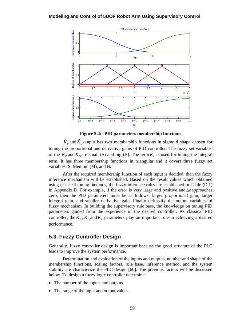
Modeling and Control of 5DOF Robot Arm Using Supervisory Control
59
Figure 5.4: PID parameters membership functions
PK and DK output has two membership functions in sigmoid shape chosen for
tuning the proportional and derivative gains of PID controller. The fuzzy set variables of the PK and DK are small (S) and big (B). The term IK is used for tuning the integral
term. It has three membership functions in triangular and it covers three fuzzy set variables: S, Medium (M), and B.
After the required membership function of each input is decided, then the fuzzy inference mechanism will be established. Based on the result values which obtained using classical tuning methods, the fuzzy inference rules are established in Table (D.1) in Appendix D. For example, if the error is very large and positive and e approaches zero, then the PID parameters must be as follows: larger proportional gain, larger integral gain, and smaller derivative gain. Finally defuzzify the output variables of fuzzy mechanism. In building the supervisory rule base, the knowledge on tuning PID parameters gained from the experience of the desired controller. As classical PID controller, the PK , DK and IK parameters play an important role in achieving a desired
performance.
5.3. Fuzzy Controller Design
Generally, fuzzy controller design is important because the good structure of the FLC leads to improve the system performance.
Determination and evaluation of the inputs and outputs, number and shape of the membership functions, scaling factors, rule base, inference method, and the system stability are characterize the FLC design [60]. The previous factors will be discussed below. To design a fuzzy logic controller determine:
The number of the inputs and outputs
The range of the input and output values
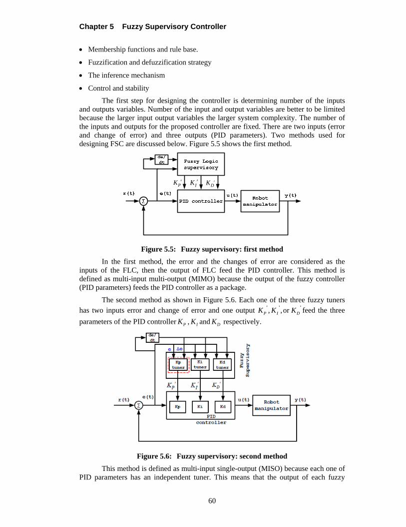
Chapter 5 Fuzzy Supervisory Controller
60
Membership functions and rule base.
Fuzzification and defuzzification strategy
The inference mechanism
Control and stability
The first step for designing the controller is determining number of the inputs and outputs variables. Number of the input and output variables are better to be limited because the larger input output variables the larger system complexity. The number of the inputs and outputs for the proposed controller are fixed. There are two inputs (error and change of error) and three outputs (PID parameters). Two methods used for designing FSC are discussed below. Figure 5.5 shows the first method.
IK DK
PK
Figure 5.5: Fuzzy supervisory: first method
In the first method, the error and the changes of error are considered as the inputs of the FLC, then the output of FLC feed the PID controller. This method is defined as multi-input multi-output (MIMO) because the output of the fuzzy controller (PID parameters) feeds the PID controller as a package.
The second method as shown in Figure 5.6. Each one of the three fuzzy tuners has two inputs error and change of error and one output ' ' ', , or P I DK K K feed the three
parameters of the PID controller PK , IK and DK respectively.
Figure 5.6: Fuzzy supervisory: second method
This method is defined as multi-input single-output (MISO) because each one of PID parameters has an independent tuner. This means that the output of each fuzzy
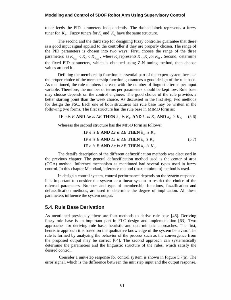
Modeling and Control of 5DOF Robot Arm Using Supervisory Control
61
tuner feeds the PID parameters independently. The dashed block represents a fuzzy tuner for PK . Fuzzy tuners for IK and DK have the same structure.
The second and the third step for designing fuzzy controller guarantee that there is a good input signal applied to the controller if they are properly chosen. The range of the PID parameters is chosen into two ways: First, choose the range of the three parameters as
min maxx x xK K K , where xK represents , ,or P I DK K K . Second, determine
the fixed PID parameters, which is obtained using Z-N tuning method, then choose values around it.
Defining the membership function is essential part of the expert system because the proper choice of the membership function guarantees a good design of the rule base. As mentioned, the rule numbers increase with the number of linguistic terms per input variable. Therefore, the number of terms per parameters should be kept low. Rule base may choose depends on the control engineer. The good choice of the rule provides a better starting point than the week choice. As discussed in the first step, two methods for design the FSC. Each one of both structures has rule base may be written in the following two forms. The first structure has the rule base in MIMO form as:
p P i I d De is E e is E k is K k is K k is K IF AND THEN AND AND (5.6)
Whereas the second structure has the MISO form as follows:
p P
i I
d D
e is E e is E k is K
e is E e is E k is K
e is E e is E k is K
IF AND THEN
IF AND THEN
IF AND THEN
(5.7)
The detail's description of the different defuzzification methods was discussed in the previous chapter. The general defuzzification method used is the center of area (COA) method. Inference mechanism as mentioned had several types used in fuzzy control. In this chapter Mamdani, inference method (max-minimum) method is used.
In design a control system, control performance depends on the system response. It is important to consider the system as a linear system to restrict the choice of the referred parameters. Number and type of membership functions, fuzzification and defuzzification methods, are used to determine the degree of implication. All these parameters influence the system output.
5.4. Rule Base Derivation
As mentioned previously, there are four methods to derive rule base [46]. Deriving fuzzy rule base is an important part in FLC design and implementation [63]. Two approaches for deriving rule base: heuristic and deterministic approaches. The first, heuristic approach it is based on the qualitative knowledge of the system behavior. The rule is formed by analyzing the behavior of the process such as the convergence from the proposed output may be correct [64]. The second approach can systematically determine the parameters and the linguistic structure of the rules, which satisfy the desired control.
Consider a unit-step response for control system is shown in Figure 5.7(a). The error signal, which is the difference between the unit step input and the output response,
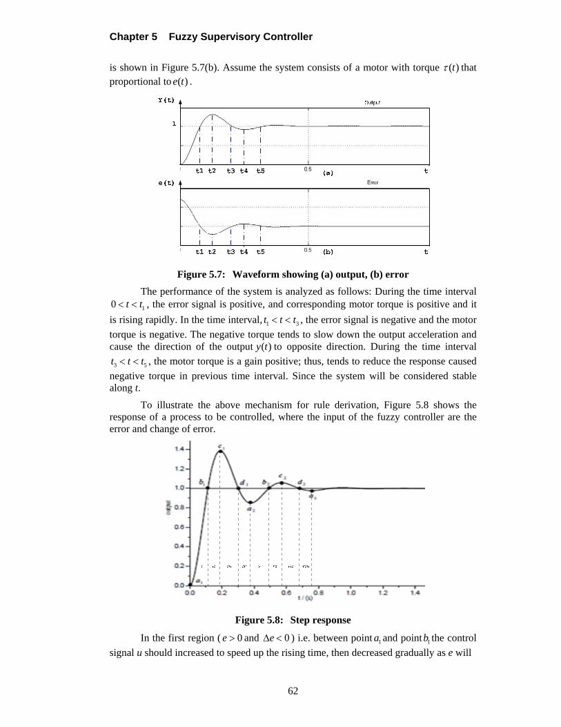
Chapter 5 Fuzzy Supervisory Controller
62
is shown in Figure 5.7(b). Assume the system consists of a motor with torque ( )t that proportional to ( )e t .
Figure 5.7: Waveform showing (a) output, (b) error
The performance of the system is analyzed as follows: During the time interval
10 t t , the error signal is positive, and corresponding motor torque is positive and it
is rising rapidly. In the time interval, 1 3t t t , the error signal is negative and the motor
torque is negative. The negative torque tends to slow down the output acceleration and cause the direction of the output ( )y t to opposite direction. During the time interval
3 5t t t , the motor torque is a gain positive; thus, tends to reduce the response caused
negative torque in previous time interval. Since the system will be considered stable along t.
To illustrate the above mechanism for rule derivation, Figure 5.8 shows the response of a process to be controlled, where the input of the fuzzy controller are the error and change of error.
Figure 5.8: Step response
In the first region ( 0e and 0e ) i.e. between point 1a and point 1b the control
signal u should increased to speed up the rising time, then decreased gradually as e will
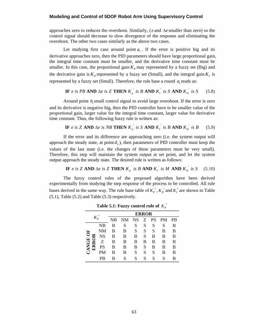
Modeling and Control of 5DOF Robot Arm Using Supervisory Control
63
approaches zero to reduces the overshoot. Similarly, (e and e smaller than zero) so the control signal should decrease to slow divergence of the response and eliminating the overshoot. The other two cases similarly as the above two cases.
Let studying first case around point 1a . If the error is positive big and its
derivative approaches zero, then the PID parameters should have large proportional gain, the integral time constant must be smaller, and the derivative time constant must be smaller. In this case, the proportional gain PK may represented by a fuzzy set (Big) and
the derivative gain is DK represented by a fuzzy set (Small), and the integral gain IK is
represented by a fuzzy set (Small). Therefore, the rule base a round 1a reads as:
' ' ' p I De is PB e is Z K is B K is S K is SIF AND THEN AND AND (5.8)
Around point 1b small control signal to avoid large overshoot. If the error is zero
and its derivative is negative big, then the PID controller have to be smaller value of the proportional gain, larger value for the integral time constant, larger value for derivative time constant. Thus, the following fuzzy rule is written as:
' ' ' p I De is Z e is NB K is S K is B K is BIF AND THEN AND AND (5.9)
If the error and its difference are approaching zero (i.e. the system output will approach the steady state, at point 2d ), then parameters of PID controller must keep the
values of the last state (i.e. the changes of these parameters must be very small). Therefore, this step will maintain the system output at set point, and let the system output approach the steady state. The desired rule is written as follows:
' ' ' p I De is Z e is Z K is B K is M K is SIF AND THEN AND AND (5.10)
The fuzzy control rules of the proposed algorithm have been derived experimentally from studying the step response of the process to be controlled. All rule
bases derived in the same way. The rule base table of PK , DK and IK are shown in Table (5.1), Table (5.2) and Table (5.3) respectively.
Table 5.1: Fuzzy control rule of PK
PK ERROR
NB NM NS Z PS PM PB
CA
NG
E O
F
ER
RO
R
NB B S S S S S B NM B B S S S B B NS B B B S B B B Z B B B B B B B
PS B B B S B B B PM B B S S S B B PB B S S S S S B
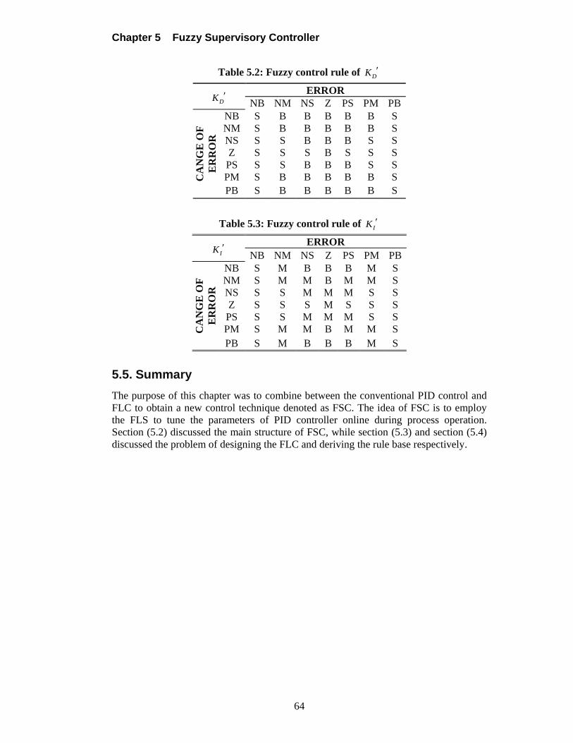
Chapter 5 Fuzzy Supervisory Controller
64
Table 5.2: Fuzzy control rule of DK
DK ERROR
NB NM NS Z PS PM PB
CA
NG
E O
F
ER
RO
R
NB S B B B B B S NM S B B B B B S NS S S B B B S S Z S S S B S S S
PS S S B B B S S PM S B B B B B S PB S B B B B B S
Table 5.3: Fuzzy control rule of IK
IK ERROR
NB NM NS Z PS PM PB
CA
NG
E O
F
ER
RO
R
NB S M B B B M S NM S M M B M M S NS S S M M M S S Z S S S M S S S
PS S S M M M S S PM S M M B M M S PB S M B B B M S
5.5. Summary
The purpose of this chapter was to combine between the conventional PID control and FLC to obtain a new control technique denoted as FSC. The idea of FSC is to employ the FLS to tune the parameters of PID controller online during process operation. Section (5.2) discussed the main structure of FSC, while section (5.3) and section (5.4) discussed the problem of designing the FLC and deriving the rule base respectively.
Modeling and Control of 5DOF Robot Arm Using Supervisory Control
65
CHAPTER 6 RESULTS
6.1. Introduction
Implementation of the proposed controllers for the robot arm has been presented in the previous three chapters. In this chapter, the results will be discussed. MATLAB and SIMULINK are used to simulate and evaluate the performance of the proposed controllers that applied on the robot. The three types of control algorithms are PID controller, FLC, and FSC are implemented to control the 5DOF robot arm using an independent joint control mechanism. The purpose of the three controllers is to improve the performance of the robot arm to acquire the desired tasks.
6.2. Lynx6 as Case Study
The proposed controllers will be used to control the Lynx 6 robot arm as a case study. Lynx6 is an articulated manipulator RRR, with 5DOF, 5 rotational joints. The robot mounted with moving gripper at the end of the chain. Figure 6.1 shows the Lynx6 robot arm.
Figure 6.1: Lynx6 robot arm
(Source: http: //www.lynxmotion.com)
The 5 joints are namely as the base, shoulder, elbow, wrist, and gripper designed to catch and hold work pieces respectively. A dedicated servomotor controls each of these joints; these motors are connected to a serial servo controller card (SSC32) to control the Lynx 6 from a computer through the serial port.
As mentioned previously, this thesis was discussed the method to model and controls the different kinds of robot manipulator without regarding to the number of joint variable and its types. Lynx6 robot arm was chosen as a case study due to its small size, lightweight, and it is inexpensive unlike industrial robots such as PUMA 560. In addition, if any kind of robot manipulator available the modeling procedure will be the same. Figure 6.2 depicts a geometric model for the Lynx 6 robot arm, which will be used for its kinematics derivation. The joint angles of Lynx6 are 1 2 3 4, , , and 5 .
Chapter 6 Results
66
Figure 6.2: Frame assignment for the Lynx 6 robot arm.
Lynx6 robot arm contains six servomotors as seen in Figure 6.1. Table (6.1) gives joint names and the combination of actuators that control the movements of these joints.
Table 6.1: Arm joints and actuators
Joint name Actuators Shoulder rotation HS-442 Shoulder 2x HS-442 Elbow HS-442 Wrist HS-442 Wrist rotation HS-81 Gripper HS-81
Table (6.2) shows the DH parameters of Lynx6 robot arm. By using the equations derived in the Chapter 2, mathematical derivation of the forward kinematic and inverse kinematic of the Lynx6 robot arm is obtained in Appendix A.
Table 6.2: DH parameter of Lynx6 robot arm
Link Joint ia i id i
1 0-1 0 90o 8 cm 1
2 1-2 12 cm 0 0 2
3 2-3 12 cm 0 0 3
4 3-4 6 -90o 0 4
5 4-5 0 0 6 cm 5
For testing the 5DOF Lynx6 robot arm, the joint desired input angles are {120 ,66 ,100 , 45 ,15 } , with initial position of the robot arm is the home
position int {0 ,0 ,0 ,0 ,0 } . Figure 6.3 shows the home position for the Lynx6 and
Figure 6.4 shows the final configuration for the input joint variables.

Modeling and Control of 5DOF Robot Arm Using Supervisory Control
67
Figure 6.3: Lynx6 home position
Figure 6.4: Lynx6 desired position
In order to assess the efficacy of the proposed controller, simulation studies have been conducted to check the efficiency of the system. PID controller is tested as the first attempt to control the Lynx6 robot arm.
Figure 6.5, Figure 6.6 and Figure 6.7 show the output response of the motors of the 5DOF Lynx6 using PID controllers.
Chapter 6 Results
68
Figure 6.5: PID control step response for 1 2,
Figure 6.6: PID control step response for 3
Modeling and Control of 5DOF Robot Arm Using Supervisory Control
69
Figure 6.7: PID control step response for 4 5and
Table (6.3) tabulated the performance of the five motors using PID controller.
Table 6.3: Performance of the PID controller
Motor number
System characteristics
Overshoot( .O S )Rising
Time( rt ) sec Steady state
error ( . .S S E )
Motor one 0.03 0.246 0.03 Motor two 0.008 0.247 0.001 Motor three 0.06 0.274 0.005 Motor four 0.02 0.277 0.01 Motor five 0.01 0.21 0.002
Effect of disturbance is studied by performing simulation of the control system in the presence of the disturbance. The disturbance is considered as the load torque that applied to the motor for each joint. The type of disturbance used in the simulation is
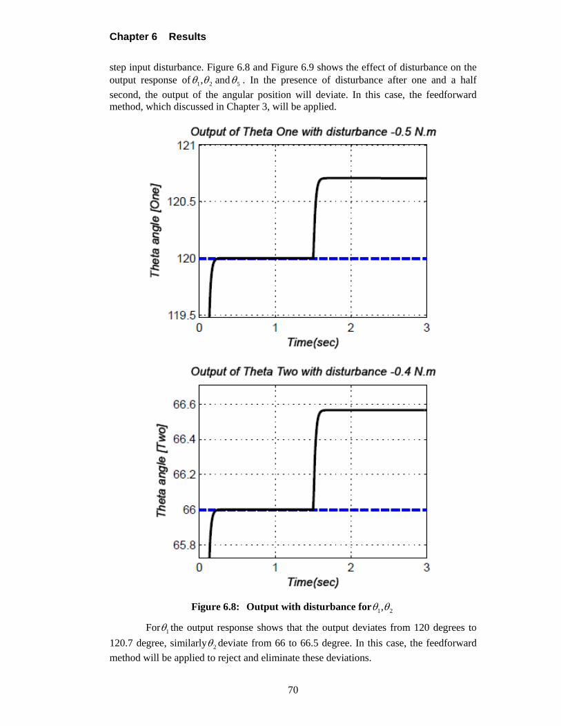
Chapter 6 Results
70
step input disturbance. Figure 6.8 and Figure 6.9 shows the effect of disturbance on the output response of 1 2, and 5 . In the presence of disturbance after one and a half
second, the output of the angular position will deviate. In this case, the feedforward method, which discussed in Chapter 3, will be applied.
Figure 6.8: Output with disturbance for 1 2,
For 1 the output response shows that the output deviates from 120 degrees to
120.7 degree, similarly 2 deviate from 66 to 66.5 degree. In this case, the feedforward
method will be applied to reject and eliminate these deviations.
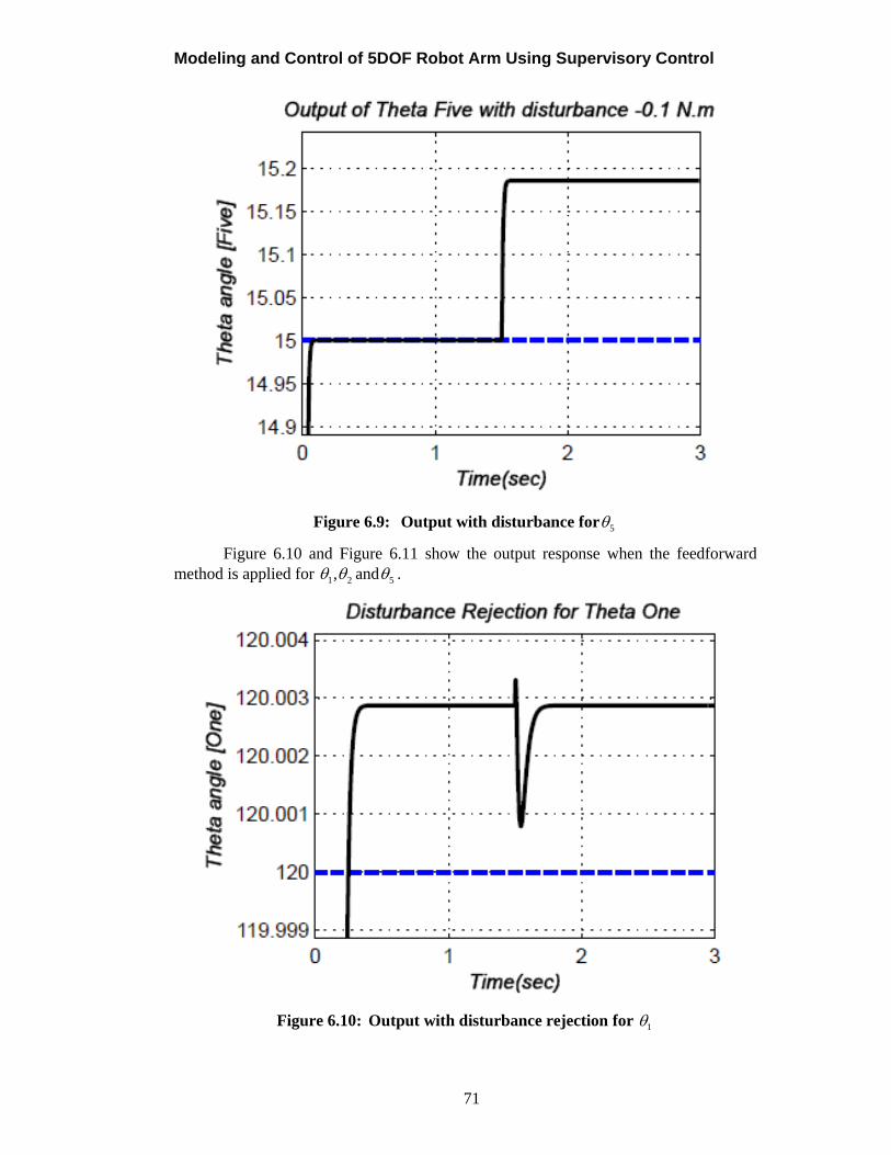
Modeling and Control of 5DOF Robot Arm Using Supervisory Control
71
Figure 6.9: Output with disturbance for 5
Figure 6.10 and Figure 6.11 show the output response when the feedforward method is applied for 1 2, and 5 .
Figure 6.10: Output with disturbance rejection for 1
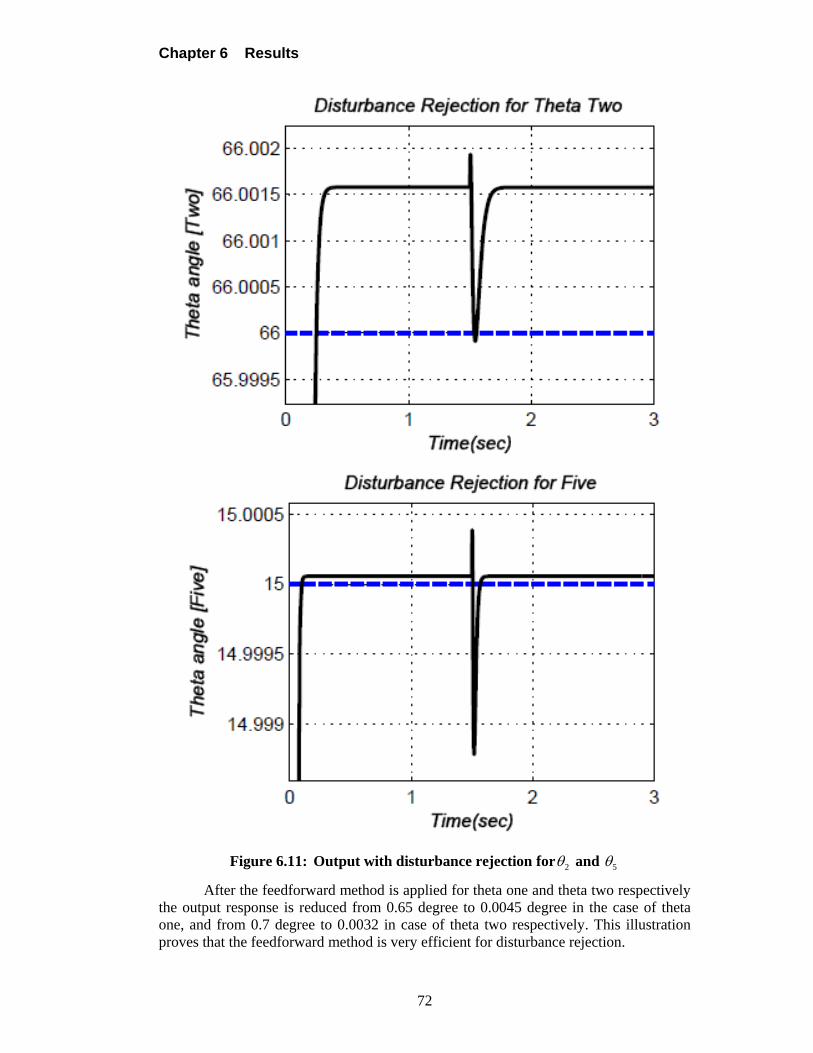
Chapter 6 Results
72
Figure 6.11: Output with disturbance rejection for 2 and 5
After the feedforward method is applied for theta one and theta two respectively the output response is reduced from 0.65 degree to 0.0045 degree in the case of theta one, and from 0.7 degree to 0.0032 in case of theta two respectively. This illustration proves that the feedforward method is very efficient for disturbance rejection.
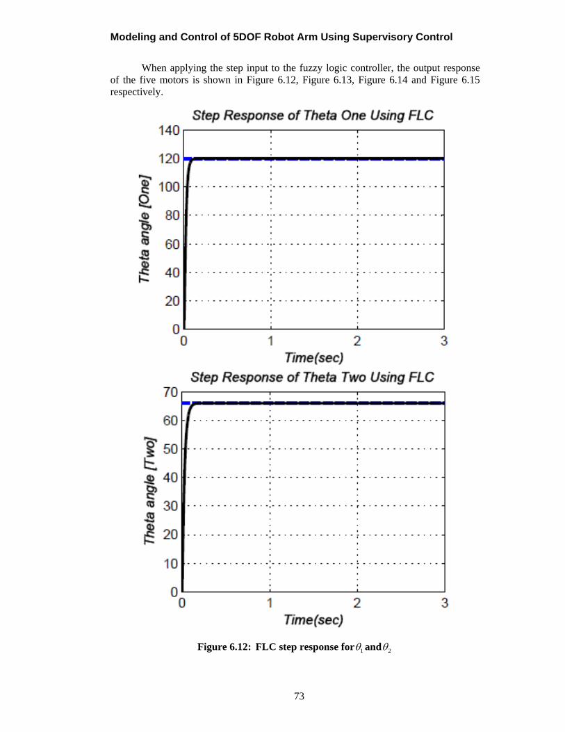
Modeling and Control of 5DOF Robot Arm Using Supervisory Control
73
When applying the step input to the fuzzy logic controller, the output response of the five motors is shown in Figure 6.12, Figure 6.13, Figure 6.14 and Figure 6.15 respectively.
Figure 6.12: FLC step response for 1 and 2

Chapter 6 Results
74
Figure 6.13: FLC step response for 3
Figure 6.14: FLC step response for 4
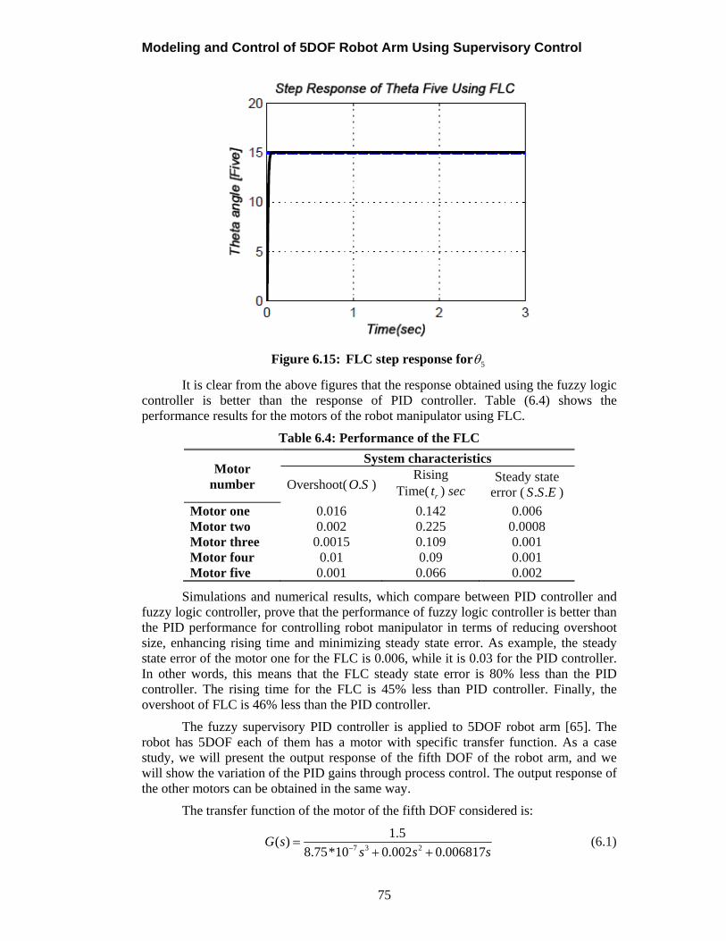
Modeling and Control of 5DOF Robot Arm Using Supervisory Control
75
Figure 6.15: FLC step response for 5
It is clear from the above figures that the response obtained using the fuzzy logic controller is better than the response of PID controller. Table (6.4) shows the performance results for the motors of the robot manipulator using FLC.
Table 6.4: Performance of the FLC
Motor number
System characteristics
Overshoot( .O S )Rising
Time( rt ) sec Steady state
error ( . .S S E )
Motor one 0.016 0.142 0.006 Motor two 0.002 0.225 0.0008 Motor three 0.0015 0.109 0.001 Motor four 0.01 0.09 0.001 Motor five 0.001 0.066 0.002
Simulations and numerical results, which compare between PID controller and fuzzy logic controller, prove that the performance of fuzzy logic controller is better than the PID performance for controlling robot manipulator in terms of reducing overshoot size, enhancing rising time and minimizing steady state error. As example, the steady state error of the motor one for the FLC is 0.006, while it is 0.03 for the PID controller. In other words, this means that the FLC steady state error is 80% less than the PID controller. The rising time for the FLC is 45% less than PID controller. Finally, the overshoot of FLC is 46% less than the PID controller.
The fuzzy supervisory PID controller is applied to 5DOF robot arm [65]. The robot has 5DOF each of them has a motor with specific transfer function. As a case study, we will present the output response of the fifth DOF of the robot arm, and we will show the variation of the PID gains through process control. The output response of the other motors can be obtained in the same way.
The transfer function of the motor of the fifth DOF considered is:
7 3 2
1.5( )
8.75*10 0.002 0.006817G s
s s s
(6.1)
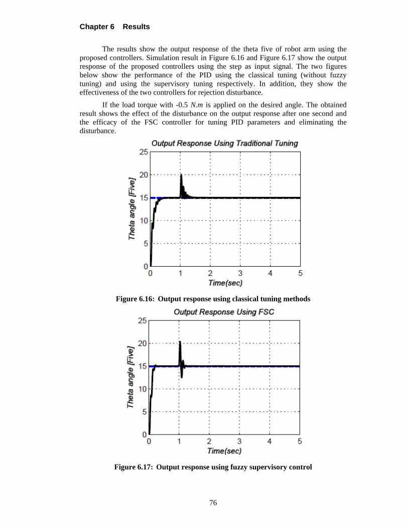
Chapter 6 Results
76
The results show the output response of the theta five of robot arm using the proposed controllers. Simulation result in Figure 6.16 and Figure 6.17 show the output response of the proposed controllers using the step as input signal. The two figures below show the performance of the PID using the classical tuning (without fuzzy tuning) and using the supervisory tuning respectively. In addition, they show the effectiveness of the two controllers for rejection disturbance.
If the load torque with -0.5 N.m is applied on the desired angle. The obtained result shows the effect of the disturbance on the output response after one second and the efficacy of the FSC controller for tuning PID parameters and eliminating the disturbance.
Figure 6.16: Output response using classical tuning methods
Figure 6.17: Output response using fuzzy supervisory control
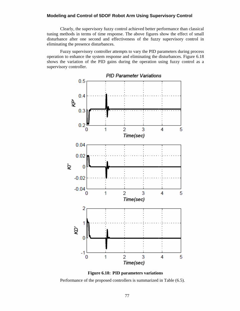
Modeling and Control of 5DOF Robot Arm Using Supervisory Control
77
Clearly, the supervisory fuzzy control achieved better performance than classical tuning methods in terms of time response. The above figures show the effect of small disturbance after one second and effectiveness of the fuzzy supervisory control in eliminating the presence disturbances.
Fuzzy supervisory controller attempts to vary the PID parameters during process operation to enhance the system response and eliminating the disturbances. Figure 6.18 shows the variation of the PID gains during the operation using fuzzy control as a supervisory controller.
Figure 6.18: PID parameters variations
Performance of the proposed controllers is summarized in Table (6.5).
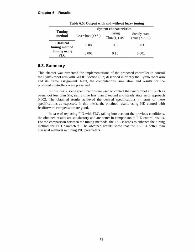
Chapter 6 Results
78
Table 6.5: Output with and without fuzzy tuning
Tuning method
System characteristics
Overshoot( .O S )Rising
Time( rt ) sec Steady state
error ( . .S S E )
Classical tuning method
0.08 0.3 0.03
Tuning using FLC
0.001 0.15 0.001
6.3. Summary
This chapter was presented the implementations of the proposed controller to control the Lynx6 robot arm with 5DOF. Section (6.2) described in briefly the Lynx6 robot arm and its frame assignment. Next, the computations, simulation and results for the proposed controllers were presented.
In this thesis, some specifications are used to control the lynx6 robot arm such as overshoot less than 5%, rising time less than 2 second and steady state error approach 0.002. The obtained results achieved the desired specifications in terms of these specifications as expected. In this thesis, the obtained results using PID control with feedforward compensator are good.
In case of replacing PID with FLC, taking into account the previous conditions, the obtained results are satisfactory and are better in comparison to PID control results. For the comparison between the tuning methods, the FSC is tends to enhance the tuning method for PID parameters. The obtained results show that the FSC is better than classical methods in tuning PID parameters.
Modeling and Control of 5DOF Robot Arm Using Supervisory Control
79
CHAPTER 7 CONCLUSION AND FUTURE WORK
7.1. Conclusion
Robotics has become recently an interesting area of research. In this thesis, we study the robot manipulator from two sides: modeling and control. Modeling process includes kinematic analysis and DC motor modeling. This process is important before controlling the robot to save the robot from being damaged. Appling a control technique is important to guarantee high efficiency and lower error for the motion of the robot.
The desired tasks were accomplished using three stages: the first stage was to provide systematic rules for analyzing forward and inverse kinematics solutions for the robot manipulator with revolute or prismatic joints using DH parameters, then analyzing the mathematical model of the DC motor in both frequency and time domains. In the second stage, we discussed the problem of control techniques. PID controller was applied, to control the robot manipulator, then FLC was implemented and considered as a second choice to control the robot. The third controller was a hybrid one between the previous controllers, denoted as FSC. In the third stage, we compared the results of using the three controllers for controlling the robot manipulator. First, we compared the results of the PID and the FLC techniques in terms of overshoot, transient response and steady state error. Second, we compared the results of PID classical tuning methods and fuzzy supervisory tuning method. All simulations were presented using MATLAB and SIMULINK, which are used widely in control applications.
The objective of this thesis was to control Lynx6 robot arm to reach the specified location with minimum error while meeting certain specification. The tracking path from the initial position to the final position was not considered in this thesis; we set the final position for each motor used independent joint control method. This thesis used the PID controller to compare its results with FLC and FSC. Feedforward method was used to overcome the disturbances, which loaded on each motor. The system was model as 5DOF, which means it has five motors to control their positions independently. In this thesis, we applied Mamdani method in FLC. This was applied using 30 rules to control robot arm. Tuning PID parameters was accomplished using FSC using 49 rules in order to fine tune KP, KI, and KD of the PID controller. By doing so, we overcame the tuning limitation of PID parameters using classical tuning methods. Both controllers used the center of area defuzzification method, and min max inference mechanism.
The simulations and numerical results of the previous controllers were presented in this thesis. We proved that the FLC is more efficient in the time response behavior than the PID controller. The average steady state error for the five motors for the FLC was 0.0105 while it was 0.042 for PID controller, in other words, the FLC steady state error is 0.75% less than the PID steady state error. We also showed that the rising time for the FLS was 49.6% less than the PID controller. The overshoot size for FLC was 73% less than the PID controller. On the other side, we proved that the FSC is more efficient to control the robot arm to reach the desired output compared to classical tuning methods. Whereas the steady state error of motor five was minimized from 0.03 to 0.001, overshoot size reduced from 0.08 to 0.001and the rising time for the FSC was 50% less than PID controller. These numerical results showed that the FSC gives satisfactory results in tuning PID parameters compared to traditional methods. To summarize, the obtained results achieved the desired performance in terms of reducing time response as expected.
Chapter 7 Conclusion and Future Work
80
7.2. Future work
A good research problem in mind is to study different fuzzy approaches. Mamdani approach may be replaced by Takagi-Sugeno model and compared with Mamdani.
This thesis recommends applying other type of inputs like cubic trajectory.
In future, we will search for methods to extract the optimum rule base to control DC motor automatically. We also apply different method of inference mechanism and defuzzification methods.
In the proposed design, we completely used off-line simulation. It can be extended to an on-line controlling for any serial robot manipulator.
The work done in this thesis was based on having PID control structure. Since the system is nonlinear, it would be interesting to apply nonlinear controllers such sliding mode control algorithms.
Modeling and Control of 5DOF Robot Arm Using Supervisory Control
81
REFERENCES
[1] M.W. Spong, S. Hutchinson and M. Vidyasagar, Robot Modeling and Control, 1st Edition, Jon Wiley & Sons, Inc, 2005.
[2] J. Angeles, Fundamentals of Robotic Mechanical Systems: Theory, Methods, and Algorithms, 2nd Edition, Springer, 2003.
[3] J.J. Crage, Introduction to Robotics Mechanics and Control, 3rd Edition, Prentice Hall, 2005.
[4] K. H. Kalil, Nonlinear Systems, 3rd Edition, Prentice-Hall, 2002. [5] R. Gorez, “A Survey of PID Auto-Tuning Methods,” Journal A, Vol. 38, No. 1,
pp. 3–10, 1997. [6] K.J. Astrom and T. Hagglund, PID Controllers: Theory, Design and Tuning, 2nd
Edition, Research Triangle Park, NC: Instrument Society of America, 1995. [7] J.G. Ziegler and N.B. Nichols, “Optimum Settings for Automatic Controllers,”
Transaction American Society of Mechanical Engineering., Vol. 64, pp. 759–768, 1942.
[8] L.A. Zadeh, “Fuzzy Sets,” Information and Control., Vol. 8, pp. 335–353, 1965. [9] E.H. Mamdani, “Applications of fuzzy logic to approximate reasoning using
linguistic synthesis,” IEEE Transactions on Computers, Vol. 26, No. 12, pp. 1182–1191, Dec. 1977.
[10] G.K.I. Mann, B.-G. Hu, and R.G. Gosine, “Analysis of Direct Action Fuzzy PID Controller Structures,” IEEE Transactions on Systems, Man, and Cybernetics, Part B, Vol. 29, No. 3, pp. 371–388, Jun. 1999.
[11] Z.-Y. Zhao, M. Tomizuka and S. Isaka, “Fuzzy Gain Scheduling PID Controller,” IEEE Transactions on Systems, Man., Cybernetics Society, Vol. 23, No. 5, pp. 1392–1398, Sep/Oct. 1993.
[12] A. Visioli, “Tuning of PID Controllers with Fuzzy Logic,” IEEE Proceedings Control Theory and Applications., Vol. 148, No. 1, pp. 1-8, 2001.
[13] X. Wang, X. Chen, W. Jia, Y. Sun and H. Pu, “Forward Kinematics Analysis and 3-Dimmision Gait Simulation of a MiniQuad Walking Robot,” IEEE International Conference on Mechatronics and Automation, pp. 1932–1937, Aug. 2007.
[14] S. Annand, Software for Control and Dynamic Simulation of Unimate Puma 560 Robot, MS Thesis, The Faculty of the College of Engineering and Technology, Ohio University, June 1993.
[15] S. Elgazzar, “Efficient Kinematic Transformations for the Puma 560 Robot,” IEEE Journal of Robotics and Automation., Vol. 1, No. 3, pp. 142–151, 1985.
[16] A.C. Soh, E.A. Alwi, R.Z. Abdul Rahman and L.H. Fey, “Effect of Fuzzy Logic Controller Implementation on a Digitally Controlled Robot Movement,” Kathmandu University Journal of Science, Engineering and Technology., Vol. I, No. V, pp 28–39, Sep. 2008.
[17] D.P. Kwok, Z.Q. Sun and P. Wang, “Linguistic PID Controller for Robot Arms,” IEEE International Conference, Vol. 1, pp. 341–346, Mar. 1991.
[18] G.M. Khoury, M. Saad, H.Y. Kanaan and C. Asmar, “Fuzzy PID Control of a Five DOF Robot Arm,” Journal of Intelligent and Robotic systems., Vol. 40, No. 3, pp.299–320, 2004.
[19] S.G. Anavatti, S.A. Salman and J.Y. Choi, “Fuzzy + PID Controller for Robot Manipulator,” International Conference on Computational Intelligence for Modelling Control and Automation., pp. 75, Dec. 2006.

References
82
[20] B.W. Bekit, L.D. Seneviratne, J.F. Whidborne and K. Althoefer, “Fuzzy PID Tuning for Robot Manipulators,” IEEE Industrial Electronics Society, in 24th Annual Conference., Vol. 4, pp. 2452–2457, Sep. 1998.
[21] B. Koyuncu and M. Güzel, “Software Development for the Kinematic Analysis of a Lynx 6 Robot Arm,” Proceedings of World Academy of Science, Engineering and Technology., Oct. 2007.
[22] O. Gürdal, M. Albayrak and T. Aydogan, “Computer Aided Control and Simulation of Robot Arm Moving in Three Dimension,” Gazi University and Suleiman Demirel University., Turkey.
[23] A.Y. -Nones, “Heterogeneous Modeling & Design of Robot Arm Control System,” University of Puerto Rico, 2004.
[24] A. Delibasi, T. Türker and G. Cansever, “Real Time Dc Motor Position Control by Fuzzy Logic and PID Controllers Using Labview,”
[25] R.E. Samin, M.S. Ramli and M.A. Ahmad, “Performance Comparison of PD-type Fuzzy Logic Controller of USBM Simplified Model,” Proceedings of The 2nd International Power Engineering and Optimization Conference., pp. 217–221, 2008.
[26] W. Li, "Design of a Hybrid Fuzzy Logic Proportional plus Conventional Integral-Derivative Controller", IEEE Transaction on Fuzzy Systems., Vo1. 6, No. 4, pp.449–463, Nov 1998.
[27] Y.C. Yung and C.Y. Chen, “PD type vs. PID type Fuzzy Controller,” IEEE 10th Region Conference Melbourne, Australia., Vol.1, pp. 341-345, Nov. 1992.
[28] S. Chopra, R. Mitra and V. Kumar, “Fuzzy Controller: Choosing an Appropriate and Smallest Rule Set,” International Journal of Computational Cognition, Vol. 3, No. 4, Dec.2005.
[29] N. Khong, A. Kanch, S. Nopna, S. Tanut, S. Tuny and R. Kagawa, “Control of the Position Dc Servo Motor by Fuzzy Logic,” IEEE Proceedings of TENCON., Vol. 3, pp.354–357, Sep.2000.
[30] A.G. Sreenatha and P. Makarand, “Fuzzy Logic Controller for Position Control of Flexible Structures,” Acta Astronaut journal., Vol. 50, No. 11, pp. 665–671, 2002.
[31] J.S. Surdhar and A.S. White, “A Parallel Fuzzy-Controlled Flexible Manipulator Using Optical Tip Feedback,” Journal of Robotics and Computer Integrated Manufacturing, Vol. 19, No. 3, pp. 273–282, 2002.
[32] M. Nil, U. Yuzgec, M. Sonmez and B. Cakir, “Fuzzy Neural Network Based Intelligent Controller For 3-DOF Robot Manipulators,” the 5th International Symposium on Intelligent Manufacturing Systems., pp. 884–895, May.2006.
[33] R.P. Copeland and K.S. Rattan, “A Fuzzy Logic Supervisor for PID Control of Unknown Systems,” IEEE International Symposium on Intelligent Control., pp. 22–26, Aug.1994.
[34] M. Dotoli, B. Maione and B. Turchiano, “Fuzzy-Supervised PID Control: Experimental Results,” EUNITE the 1st European Symposium on Intelligent Technologies, Hybrid Systems and their Implementation on Smart Adaptive Systems, pp. 31–35, 2001
[35] L. Wang, M. Tian and Y. Gao, “Fuzzy Self-adapting PID Control of PMSM Servo System,” IEEE International Electric Machines & Drives Conference., Vol. 1, pp. 860–863, May.2007.
[36] K.K. Ahn and N.B. Kha, “Position Control of Shape Memory Alloy Actuators Using Self Tuning Fuzzy PID Controller,” IEEE Conference on Industrial Electronics and Applications., pp. 1–5, May.2006.
Modeling and Control of 5DOF Robot Arm Using Supervisory Control
83
[37] S.G. Tzafestas and N.P. Papanikolopoulos, “Incremental fuzzy expert PID Control,” IEEE Transactions on Industrial Electronics., Vol. 37, No. 5, pp. 365–371, Oct.1990.
[38] K.H. Ang, G.C.Y. Chong, and Y. Li, “PID Control System Analysis, Design, and Technology,” IEEE Transactions on Control Systems Technology., Vol. 13, No. 4, pp. 559–576, July.2005.
[39] C.K. Benjamin, Automatic Control System, 7th Edition, Englewood Cliffs, Prentice Hall, pp. 175–180, 1995.
[40] Z.-Y. Zhao, M. Tomizuka and S. Isaka, “Fuzzy Gain Scheduling of PID Controllers,” IEEE Conference on Control Applications., Vol. 2, pp. 698–703, Sep.1992.
[41] C.C. Hang, K.J. Astrom, and W.K. Ho, “Refinements of the Ziegler–Nichols Tuning Formula,” IEE Proceedings D Control Theory and Applications., Vol. 138, No. 2, pp. 111–118, Mar. 1991.
[42] T.C. Chi, Analog and Digital Control System Design: Transfer-Function, State-Space, and Algebraic Methods, Saunders College, pp. 551–563, 1993.
[43] N.S. Nise, Control System Engineering, 4th Edition, Wiley, 2004. [44] S.W. Zhao and N.C. Cheung, “Disturbances Rejection for Precise Position
Control of Linear Switched Reluctance Motors,” Proceedings of the 17th World Congress the International Federation of Automatic Control, July. 2008.
[45] G. Feng, “A Survey on Analysis and Design of Model-Based Fuzzy Control Systems,” IEEE Transactions on Fuzzy Systems., Vol. 14, No. 5, pp. 676–697, Oct. 2006.
[46] C.C. Lee, “Fuzzy Logic in Control Systems: Fuzzy Logic Controller-Part I”, IEEE Transactions on Systems, Man and Cybernetics., Vol. 20, No.2, pp. 404–418, March/April 1990.
[47] M. Sugeno, “An Introductory Survey of Fuzzy Control,” Information Sciences., 36, pp. 59–83, 1995.
[48] V. Kumar and A.P. Mittal, “Parallel Fuzzy P + Fuzzy I + Fuzzy D controller: Design and Performance Evaluation,” International Journal of Automation and Computing., 2009.
[49] C.C. Lee, “Fuzzy logic in control systems: Fuzzy Logic Controller-part II,” IEEE Transactions on Systems, Man and Cybernetics., Vol. 20, No.2, pp. 419–435, March/April 1990.
[50] T. Terano, K. Asia, and M. Sugeno, Fuzzy Systems Theory and its Applications, Academic Press, pp. 34–59, 1992.
[51] J. Jantzen, Foundations of Fuzzy Control, John Wiley & Sons, pp. 17-19, 2007. [52] E.H. Mamdani, H.J. Efstathiou and K. Sugiyama., “Development of Fuzzy Logic
Control,” The 23rd IEEE Conference on Decision and Control., Vol. 23, pp. 888–893, 1984.
[53] V.G. Moudgal, S. Yurkovich, and K.M. Passino, “Rule-Based Control for A Flexible-Link Robot,” IEEE Transactions on Control Systems Technology., Vol .2, No. 4, pp. 392–405, Dec.1994.
[54] H. Ying, “The Takagi-Sugeno Fuzzy Controllers Using The Simplified Linear Rules Are Nonlinear Variable Gain Controllers”, Automatica, Vol. 34, No. 2, pp. 157–167, 1998.
[55] O.A.S. Youssef, “Applications of Fuzzy Inference Mechanisms to Power System Relaying,” IEEE Power Systems Conference and Exposition., Vol. 1, pp. 560–567, Oct. 2004.
References
84
[56] S.N. Sivanandam, S. Sumathi and S.N. Deepa, Introduction to Fuzzy Logic Using MATLAB, Springer, pp. 97–107, 2007.
[57] G.K.I. Mann, B.G. Hu and R.G. Gosine, “A systematic study of fuzzy PID controllers - function-based evaluation approach,” IEEE Transactions on Fuzzy System., Vol. 9, No. 5, pp. 699–712, Oct. 2001.
[58] R. Ketata, D. De Geest, and A. Titli, “Fuzzy controllers: Design, evaluation, parallel, and hierarchical combination with a PID controllers,” Fuzzy Sets System., Vol. 71, No. 1, pp. 113–129, Apr. 1995.
[59] A.Z. Alassar, I.M. Abuhadrous and H.A. Elaydi “Control of 5DOF Robot Arm Using PID Controller with Feedforward Compensation”, Accepted in the 2nd Conference on Computer and Automation Engineering, Singapore, 5. Dec. 2009.
[60] K.-N. Luo, C.-Y. Kuo, and L.-T. Sheu, “A Novel Method for Fuzzy Self-Tuning PID Controllers,” IEEE Proceedings of the Asian Fuzzy Systems Symposium, pp. 194–199, Dec. 1996.
[61] L. Yao and C.-C. Lin, “Design of Gain Scheduled Fuzzy PID Controller,” International Conference on Computational Intelligence., pp. 432-436, Nov. 2004.
[62] Y. Yang, W. Wang, D.-J. Yu and G. Ding, “A Fuzzy Parameters Adaptive PID Controller Design of Digital Positional Servo System,” IEEE Proceeding of the First International Conference on Machine Learning and Cybernetics., Vol. 1, pp. 310–314, Nov. 2002.
[63] A.Z. Alassar, I.M. Abuhadrous and H.A. Elaydi “Comparison between FLC and PID Controller for 5DOF Robot Arm”, The 2nd IEEE International Conference on Advanced Computer Control, Shenyang, Dec. 2009.
[64] Y.-Y. Chen, “Rules Extraction for Fuzzy Control System,” IEEE international Conference on System Man and Cybernetics., Vol. 2, pp. 526–527, Nov 1989.
[65] A.Z. Alassar, I.M. Abuhadrous and H.A. Elaydi “Modeling and Control of 5DOF Robot Arm Using Supervisory Control”, The 2nd International Conference on Computer and Automation Engineering, Singapore, Jan. 2010.
Modeling and Control of 5DOF Robot Arm Using Supervisory Control
85
PUBLICATIONS
[1] A.Z. Alassar, I.M. Abuhadrous and H.A. Elaydi “Control of 5DOF Robot Arm Using PID Controller with Feedforward Compensation”, Accepted in the 2nd Conference on Computer and Automation Engineering, Singapore, 5. Dec. 2009.
[2] A.Z. Alassar, I.M. Abuhadrous and H.A. Elaydi “Comparison between FLC and PID Controller for 5DOF Robot Arm”, The 2nd IEEE International Conference on Advanced Computer Control, Shenyang, Dec. 2009.
[3] A.Z. Alassar, I.M. Abuhadrous and H.A. Elaydi “Modeling and Control of 5DOF Robot Arm Using Supervisory Control”, The 2nd Conference on Computer and Automation Engineering, Singapore, Jan. 2010.
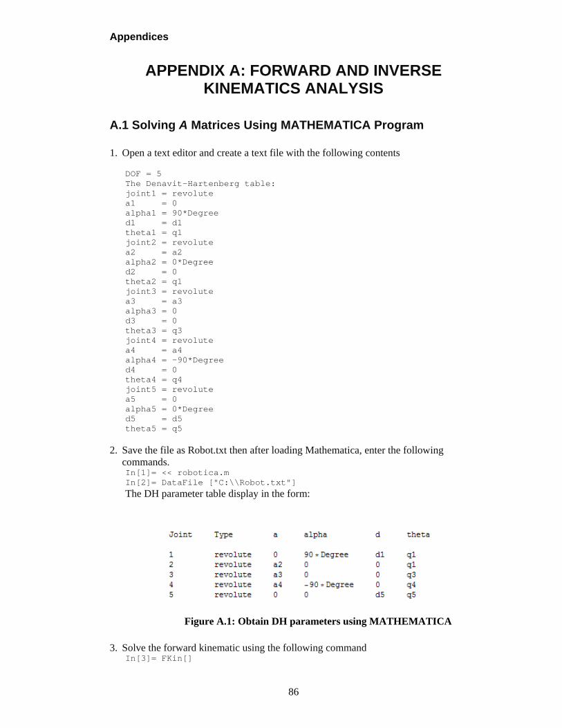
Appendices
86
APPENDIX A: FORWARD AND INVERSE KINEMATICS ANALYSIS
A.1 Solving A Matrices Using MATHEMATICA Program 1. Open a text editor and create a text file with the following contents
DOF = 5 The Denavit-Hartenberg table: joint1 = revolute a1 = 0 alpha1 = 90*Degree d1 = d1 theta1 = q1 joint2 = revolute a2 = a2 alpha2 = 0*Degree d2 = 0 theta2 = q1 joint3 = revolute a3 = a3 alpha3 = 0 d3 = 0 theta3 = q3 joint4 = revolute a4 = a4 alpha4 = -90*Degree d4 = 0 theta4 = q4 joint5 = revolute a5 = 0 alpha5 = 0*Degree d5 = d5 theta5 = q5
2. Save the file as Robot.txt then after loading Mathematica, enter the following commands. In[1]= << robotica.m In[2]= DataFile ["C:\\Robot.txt"] The DH parameter table display in the form:
Figure A.1: Obtain DH parameters using MATHEMATICA
3. Solve the forward kinematic using the following command
In[3]= FKin[]
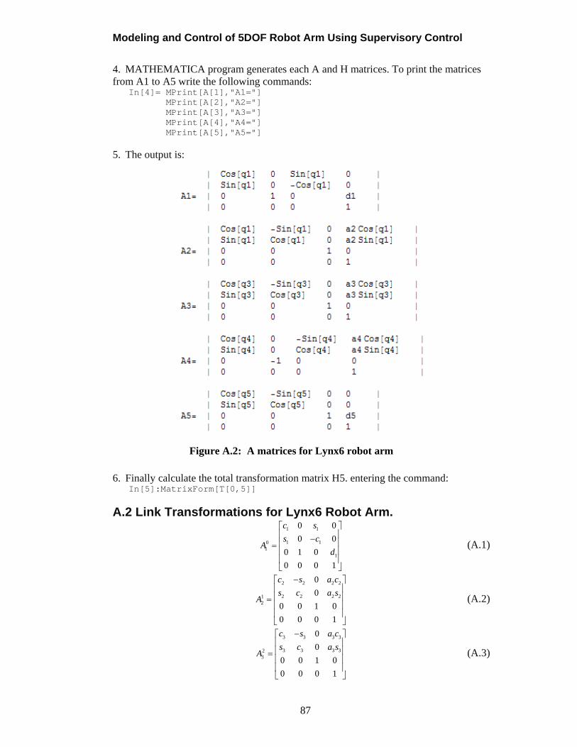
Modeling and Control of 5DOF Robot Arm Using Supervisory Control
87
4. MATHEMATICA program generates each A and H matrices. To print the matrices from A1 to A5 write the following commands:
In[4]= MPrint[A[1],"A1="] MPrint[A[2],"A2="] MPrint[A[3],"A3="] MPrint[A[4],"A4="] MPrint[A[5],"A5="]
5. The output is:
Figure A.2: A matrices for Lynx6 robot arm
6. Finally calculate the total transformation matrix H5. entering the command:
In[5]:MatrixForm[T[0,5]]
A.2 Link Transformations for Lynx6 Robot Arm.
1 1
1 101
1
0 0
0 0
0 1 0
0 0 0 1
c s
s cA
d
(A.1)
2 2 2 2
2 2 2 212
0
0
0 0 1 0
0 0 0 1
c s a c
s c a sA
(A.2)
3 3 3 3
3 3 3 323
0
0
0 0 1 0
0 0 0 1
c s a c
s c a sA
(A.3)
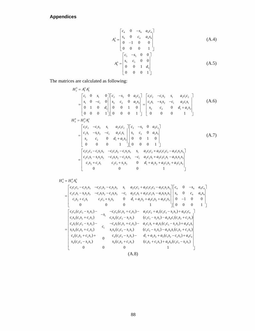
Appendices
88
4 4 4 4
4 4 4 434
0
0
0 1 0 0
0 0 0 1
c s a c
s c a sA
(A.4)
5 5
5 545
5
0 0
0 0
0 0 1
0 0 0 1
c s
s cA
d
(A.5)
The matrices are calculated as following:
0 0 12 1 2
1 1 2 2 2 2 1 2 1 2 1 2 1 2
1 1 2 2 2 2 2 1 1 2 1 2 1 1
1 2 2 1 2 2
0 0 0
0 0 0
0 1 0 0 0 1 0 0
0 0 0 1 0 0 0 1 0 0 0 1
H A A
c s c s a c c c c s s a c c
s c s c a s c s s s c a c s
d s c d a s
(A.6)
0 0 23 2 3
1 2 1 2 1 2 1 2 3 3 3 3
2 1 1 2 1 2 1 1 3 3 3 3
2 2 1 2 2
1 2 3 1 2 3 1 3 2 1 2 3 1 2 1 2 3 1 2 3 3 1 2 3
2 3 1 1 2 3 3 1 2
0
0
0 0 0 1 0
0 0 0 1 0 0 0 1
H H A
c c c s s a c c c s a c
c s s s c a c s s c a s
s c d a s
c c c c s s c c s c s s s a c c a c c c a c s s
c c s s s s c s s
2 1 3 1 2 2 1 3 3 2 1 3 1 2 3
3 2 2 1 2 3 2 3 1 2 2 3 3 2 3 2 3
0
0 0 0 1
c s s c a c s a c c s a s s s
c s c s c c s s d a s a c s a c s
(A.7)
0 0 34 3 4
1 2 3 1 2 3 1 3 2 1 2 3 1 2 1 2 3 1 2 3 3 1 2 3 4 4 4 4
2 3 1 1 2 3 3 1 2 2 1 3 1 2 2 1 3 3 2 1 3 1 2 3 4 4 4 4
3 2 2 1 2 3 2 3 1 2 2 3 3 2 3 2 3
0
0
0 0
0 0 0 1
H H A
c c c c s s c c s c s s s a c c a c c c a c s s c s a c
c c s s s s c s s c s s c a c s a c c s a s s s s c a s
c s c s c c s s d a s a c s a c s
1 4 2 3 2 3 1 4 3 2 2 3 2 1 2 3 2 3 2 3 4 1 41
1 4 3 2 2 3 1 4 2 3 2 3 2 3 2 3 4 4 1 3 2 2 3
4 1 2 3 2 3 4 1 3 2 2 31
1 4 3 2 2 3 1
1 0 0
0 0 0 1
( ) ( ) ( )
( ) ( ) ( ) ( )
( ) ( )
( )
c c c c s s c c c s c s a c c a c c s s a c cs
c s c s c s c s c c s s c c s s a s c c s c s
c s c c s s c s c s c sc
s s c s c s s s
2 2 1 3 1 2 3 2 3 4 4 1
4 2 3 2 3 2 3 2 3 4 4 1 3 2 2 3
4 3 2 2 3 4 2 3 2 3 1 2 2 3 3 2 2 3 4 4
4 2 3 2 3 4 3 2 2 3 3 2 2 3 4 4 2 3 2 3
( )
( ) ( ) ( )
( ) ( ) ( )0
( ) ( ) ( ) ( )
0 0 0 1
a c s a s c c s s a c s
c c s s c c s s a s s c s c s
c c s c s c c c s s d a s a c s c s a c
s c c s s s c s c s c s c s a s c c s s
(A.8)
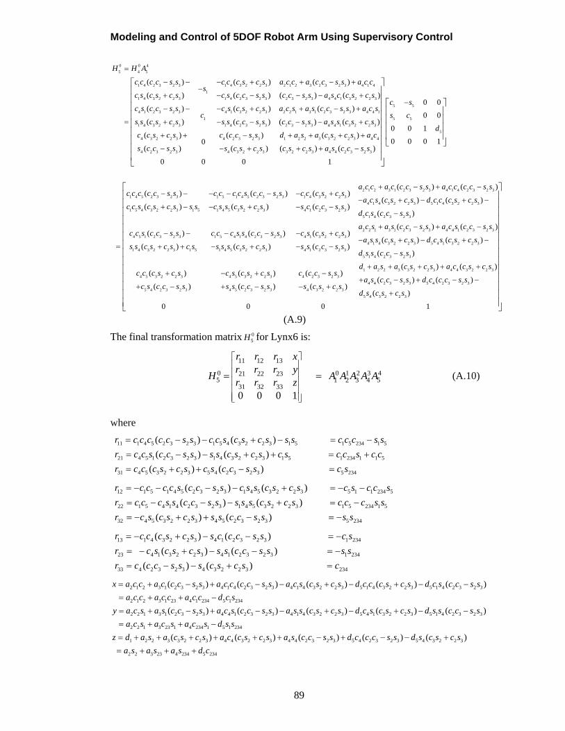
Modeling and Control of 5DOF Robot Arm Using Supervisory Control
89
0 0 4
5 4 5
1 4 2 3 2 3 1 4 3 2 2 3 2 1 2 3 2 3 2 3 4 1 4
1
1 4 3 2 2 3 1 4 2 3 2 3 2 3 2 3 4 4 1 3 2 2 3
4 1 2 3 2 3 4 1 3 2 2 3
1
1 4 3 2 2 3 1 4 2 3 2
( ) ( ) ( )
( ) ( ) ( ) ( )
( ) ( )
( ) (
H H A
c c c c s s c c c s c s a c c a c c s s a c cs
c s c s c s c s c c s s c c s s a s c c s c s
c s c c s s c s c s c sc
s s c s c s s s c c s
5 5
2 2 1 3 1 2 3 2 3 4 4 1
3 2 3 2 3 4 4 1 3 2 2 3
4 3 2 2 3 4 2 3 2 3 1 2 2 3 3 2 2 3 4 4
4 2 3 2 3 4 3 2 2 3 3 2 2 3 4 4 2 3 2 3
( )
) ( ) ( )
( ) ( ) ( )0
( ) ( ) ( ) ( )
0 0 0 1
c sa c s a s c c s s a c s
s c c s s a s s c s c s
c c s c s c c c s s d a s a c s c s a c
s c c s s s c s c s c s c s a s c c s s
5 5
5
0 0
0 0
0 0 1
0 0 0 1
s c
d
2 1 2 3 1 2 3 2 3 4 1 4 2 3 2 3
1 4 5 2 3 2 3 1 5 1 4 5 2 3 2 3 1 4 3 2 2 3
4 1 4 3 2 2 3 5 1 4 3 2 2 3
1 5 4 3 2 2 3 1 5 1 4 5 3 2 2 3 4 1 2 3 2 3
5 1
( ) ( )( ) ( ) ( )
( ) ( )( ) ( ) ( )
a c c a c c c s s a c c c c s sc c c c c s s c c c c s c c s s c c c s c s
a c s c s c s d c c c s c sc c s c s c s s s c s s c s c s s c c c s s
d c
4 2 3 2 3
2 2 1 3 1 2 3 2 3 4 4 1 2 3 2 3
4 5 1 2 3 2 3 1 5 4 1 4 2 3 2 3 4 1 3 2 2 3
4 1 4 3 2 2 3 5 4 1 3 2 2 3
1 4 3 2 2 3 1 5 1 4 5 3 2 2 3 4 1 2 3 2 3
( )
( ) ( )( ) ( ) ( )
( ) ( )( ) ( ) ( )
s c c s s
a c s a s c c s s a c s c c s sc c s c c s s c c c s s c c s s c s c s c s
a s s c s c s d c s c s c ss s c s c s c s s s s c s c s s s c c s s
5 1 4 2 3 2 3
1 2 2 3 3 2 2 3 4 4 3 2 2 3
4 5 3 2 2 3 4 5 3 2 2 3 4 2 3 2 3
4 4 2 3 2 3 5 4 2 3 2 3
5 4 2 3 2 3 4 5 2 3 2 3 4 3 2 2 3
5 4 3 2 2 3
( )
( ) ( )( ) ( ) ( )
( ) ( )( ) ( ) ( )
( )
0 0 0 1
d s s c c s s
d a s a c s c s a c c s c sc c c s c s c s c s c s c c c s s
a s c c s s d c c c s sc s c c s s s s c c s s s c s c s
d s c s c s
(A.9)
The final transformation matrix 05H for Lynx6 is:
11 12 13
0 0 1 2 3 421 22 235 51 2 3 4
31 32 33
0 0 0 1
r r r xr r r y
H A A A A Ar r r z
(A.10)
where
11 1 4 5 2 3 2 3 1 5 4 3 2 2 3 1 5 1 5 234 1 5
21 4 5 1 2 3 2 3 1 4 3 2 2 3 1 5 1 234 1 1 5
31 4 5 3 2 2 3 5 4 2 3 2 3
( ) ( )
( ) ( )
( ) ( )
r c c c c c s s c c s c s c s s s c c c s s
r c c s c c s s s s c s c s c s c c s c c
r c c c s c s c s c c s s
5 234 c s
12 1 5 1 4 5 2 3 2 3 1 4 5 3 2 2 3 5 1 1 234 5
22 1 5 4 1 4 2 3 2 3 1 4 5 3 2 2 3 1 5 234 1 5
32 4 5 3 2 2 3 4 5 2 3 2 3 5 2
( ) ( )
( ) ( )
( ) ( )
r c c c c s c c s s c s s c s c s c s c c s
r c c c s s c c s s s s s c s c s c c c s s
r c s c s c s s s c c s s s s
34
13 1 4 3 2 2 3 4 1 2 3 2 3 1 234
23 4 1 3 2 2 3 4 1 2 3 2 3 1 234
33 4 2 3 2 3 4 3 2 2 3 234
( ) ( )
( ) ( )
( ) ( )
r c c c s c s s c c c s s c s
r c s c s c s s s c c s s s s
r c c c s s s c s c s c
2 1 2 3 1 2 3 2 3 4 1 4 2 3 2 3 4 1 4 3 2 2 3 5 1 4 3 2 2 3 5 1 4 2 3 2 3
2 1 2 3 1 23 4 1 234 5 1 234
2 2 1 3 1 2 3 2 3 4 4 1 2 3 2 3 4 1 4 3 2 2 3 5 4 1
( ) ( ) ( ) ( ) ( )
( ) ( ) ( ) (
x a c c a c c c s s a c c c c s s a c s c s c s d c c c s c s d c s c c s s
a c c a c c a c c d c s
y a c s a s c c s s a c s c c s s a s s c s c s d c s c
3 2 2 3 5 1 4 2 3 2 3
2 2 1 3 23 1 4 234 1 5 1 234
1 2 2 3 3 2 2 3 4 4 3 2 2 3 4 4 2 3 2 3 5 4 2 3 2 3 5 4 3 2 2 3
2 2 3 23 4 234 5 234
) ( )
( ) ( ) ( ) ( ) ( )
s c s d s s c c s s
a c s a c s a c s d s s
z d a s a c s c s a c c s c s a s c c s s d c c c s s d s c s c s
a s a s a s d c
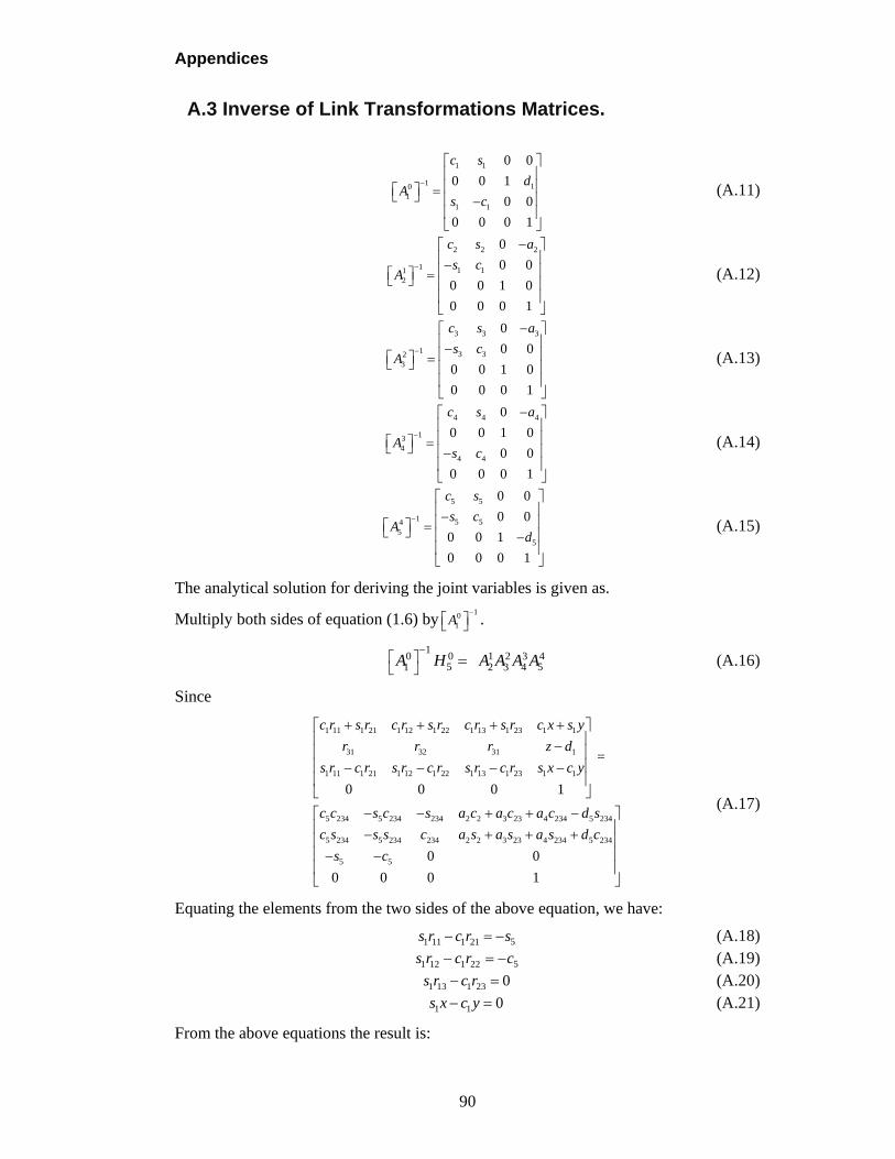
Appendices
90
A.3 Inverse of Link Transformations Matrices.
1 1
1 101
1 1
0 0
0 0 1
0 0
0 0 0 1
c s
dA
s c
(A.11)
2 2 2
1 1 112
0
0 0
0 0 1 0
0 0 0 1
c s a
s cA
(A.12)
3 3 3
1 3 323
0
0 0
0 0 1 0
0 0 0 1
c s a
s cA
(A.13)
4 4 4
134
4 4
0
0 0 1 0
0 0
0 0 0 1
c s a
As c
(A.14)
5 5
1 5 545
5
0 0
0 0
0 0 1
0 0 0 1
c s
s cA
d
(A.15)
The analytical solution for deriving the joint variables is given as.
Multiply both sides of equation (1.6) by10
1A
.
1
0 0 1 2 3 45 51 2 3 4 A H A A A A
(A.16)
Since
1 11 1 21 1 12 1 22 1 13 1 23 1 1
31 32 31 1
1 11 1 21 1 12 1 22 1 13 1 23 1 1
5 234 5 234 234 2 2 3 23 4 234 5 234
5 234 5 234 234 2 2 3 23 4 234 5 234
5 5
=
0 0 0 1
c r s r c r s r c r s r c x s y
r r r z d
s r c r s r c r s r c r s x c y
c c s c s a c a c a c d s
c s s s c a s a s a s d c
s c
0 0
0 0 0 1
(A.17)
Equating the elements from the two sides of the above equation, we have:
51 11 1 21s r c r s (A.18) 51 12 1 22s r c r c (A.19) 1 13 1 23 0s r c r (A.20) 1 1 0s x c y (A.21)
From the above equations the result is:
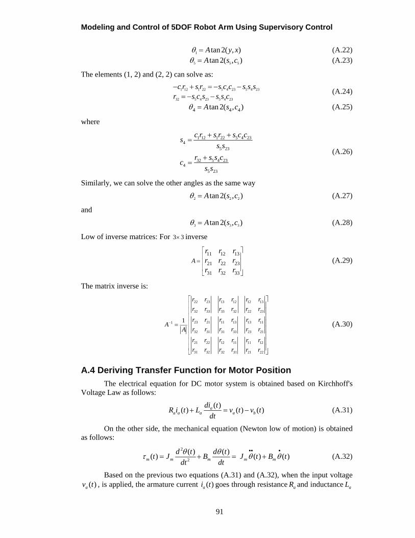
Modeling and Control of 5DOF Robot Arm Using Supervisory Control
91
1 tan 2( , )A y x (A.22) 5 5 5tan 2( , )A s c (A.23)
The elements (1, 2) and (2, 2) can solve as:
1 12 1 22 5 4 23 5 4 23
32 5 4 23 5 4 23
c r s r s c c s s sr s c s s s c
(A.24)
4 4 4tan 2( , )A s c (A.25)
where
1 12 1 22 5 4 234
5 23
32 5 4 234
5 23
c r s r s c cs
s s
r s s cc
s s
(A.26)
Similarly, we can solve the other angles as the same way
2 2 2tan 2( , )A s c (A.27)
and
3 3 3tan 2( , )A s c (A.28)
Low of inverse matrices: For 3 3 inverse
11 12 13
21 22 23
31 32 33
A
r r rr r rr r r
(A.29)
The matrix inverse is:
22 23 13 12 12 13
32 33 33 32 22 23
23 21 11 13 13 111
32 31 31 33 23 21
21 22 12 11 11 12
31 32 32 31 21 22
1
r r r r r r
r r r r r r
r r r r r rA
r r r r r rA
r r r r r r
r r r r r r
(A.30)
A.4 Deriving Transfer Function for Motor Position
The electrical equation for DC motor system is obtained based on Kirchhoff's Voltage Law as follows:
( )
( ) ( ) ( )aa a a a b
di tR i t L v t v t
dt (A.31)
On the other side, the mechanical equation (Newton low of motion) is obtained as follows:
2
2
( ) ( )( ) ( ) ( )m m m m m
d t d tt J B J t B t
dt dt
(A.32)
Based on the previous two equations (A.31) and (A.32), when the input voltage ( )av t , is applied, the armature current ( )ai t goes through resistance aR and inductance aL
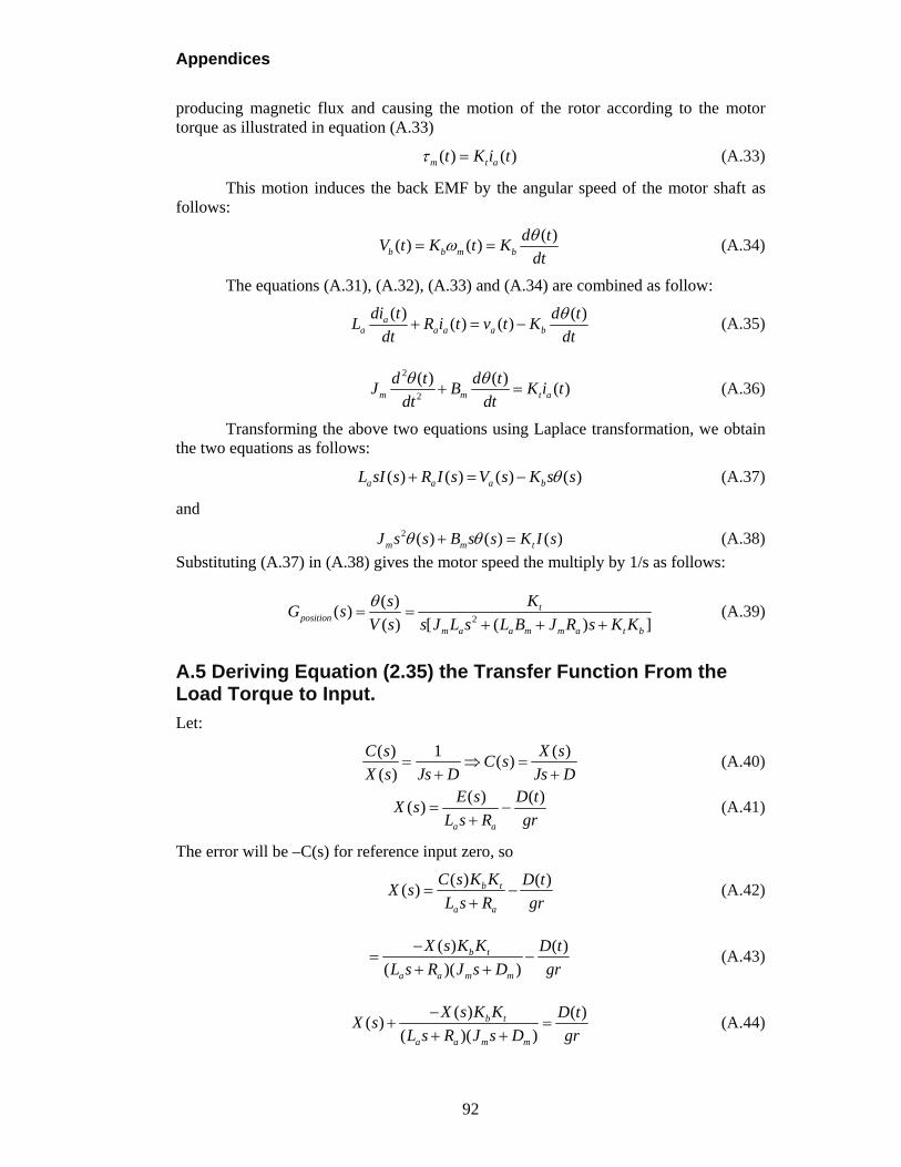
Appendices
92
producing magnetic flux and causing the motion of the rotor according to the motor torque as illustrated in equation (A.33)
( ) ( )m t at K i t (A.33)
This motion induces the back EMF by the angular speed of the motor shaft as follows:
( )
( ) ( )b b m b
d tV t K t K
dt
(A.34)
The equations (A.31), (A.32), (A.33) and (A.34) are combined as follow:
( ) ( )
( ) ( )aa a a a b
di t d tL R i t v t K
dt dt
(A.35)
2
2
( ) ( )( )m m t a
d t d tJ B K i t
dt dt
(A.36)
Transforming the above two equations using Laplace transformation, we obtain the two equations as follows:
( ) ( ) ( ) ( )a a a bL sI s R I s V s K s s (A.37)
and
2 ( ) ( ) ( )m m tJ s s B s s K I s (A.38)
Substituting (A.37) in (A.38) gives the motor speed the multiply by 1/s as follows:
2
( )( )
( ) [ ( ) ]t
positionm a a m m a t b
KsG s
V s s J L s L B J R s K K
(A.39)
A.5 Deriving Equation (2.35) the Transfer Function From the Load Torque to Input.
Let:
( ) 1 ( )
( )( )
C s X sC s
X s Js D Js D
(A.40)
( ) ( )
( )a a
E s D tX s
L s R gr
(A.41)
The error will be –C(s) for reference input zero, so
( ) ( )
( ) b t
a a
C s K K D tX s
L s R gr
(A.42)
( ) ( )
( )( )b t
a a m m
X s K K D t
L s R J s D gr
(A.43)
( ) ( )
( )( )( )
b t
a a m m
X s K K D tX s
L s R J s D gr
(A.44)
Modeling and Control of 5DOF Robot Arm Using Supervisory Control
93
( )
( )1
( )( )b t
a a m m
D t grX s
K K
L s R J s D
(A.45)
( ) 1( )( ) 1
( ) ( )
b t
a a m m
m m
K KgrC s
L s R J s D
D t J s D
(A.46)
( ) 1
( )( ) 1
( )( )b t
m ma a m m
grC s
D t K KJ s D
L s R J s D
(A.47)
( )( )
( ) ( )( )a a
a a m m b t
L s R grC s
D t L s R J s D K K
(A.48)
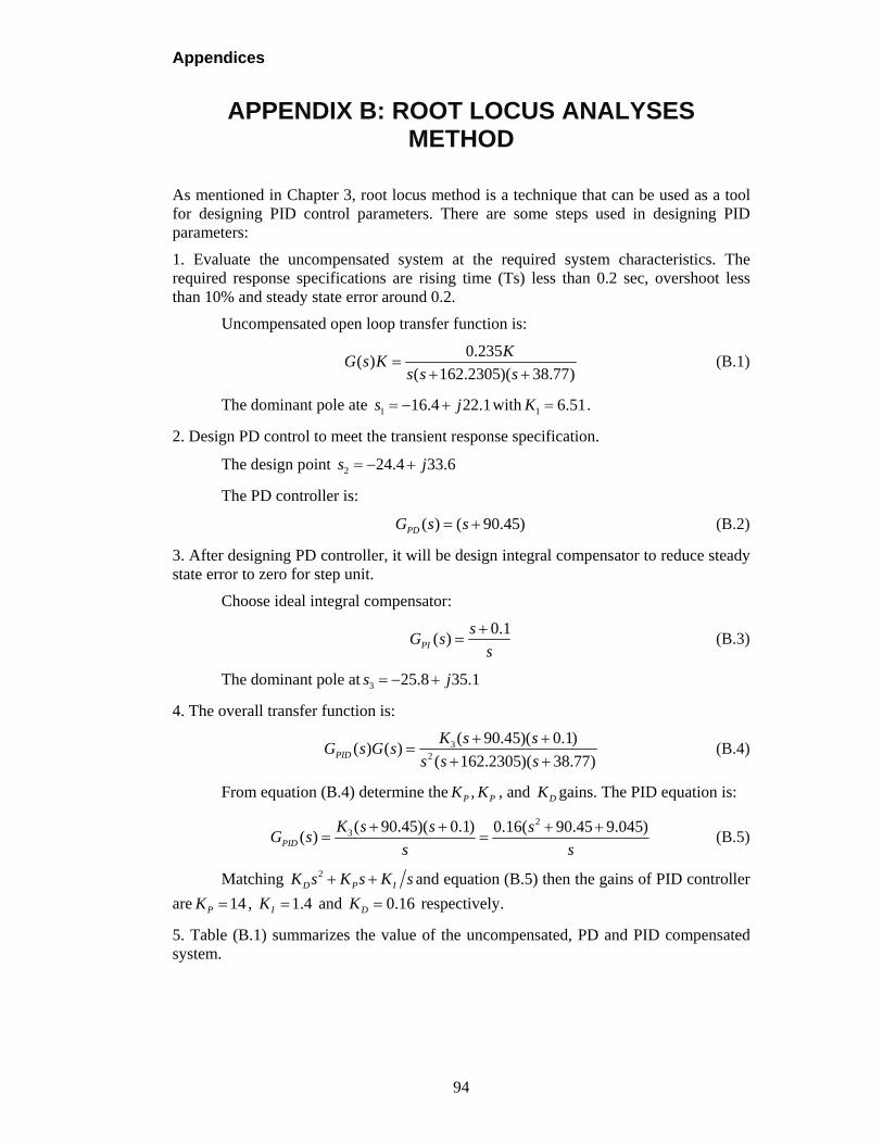
Appendices
94
APPENDIX B: ROOT LOCUS ANALYSES METHOD
As mentioned in Chapter 3, root locus method is a technique that can be used as a tool for designing PID control parameters. There are some steps used in designing PID parameters:
1. Evaluate the uncompensated system at the required system characteristics. The required response specifications are rising time (Ts) less than 0.2 sec, overshoot less than 10% and steady state error around 0.2.
Uncompensated open loop transfer function is:
0.235
( )( 162.2305)( 38.77)
KG s K
s s s
(B.1)
The dominant pole ate 1 16.4 22.1s j with 1 6.51K .
2. Design PD control to meet the transient response specification.
The design point 2 24.4 33.6s j
The PD controller is:
( ) ( 90.45)PDG s s (B.2)
3. After designing PD controller, it will be design integral compensator to reduce steady state error to zero for step unit.
Choose ideal integral compensator:
0.1
( )PI
sG s
s
(B.3)
The dominant pole at 3 25.8 35.1s j
4. The overall transfer function is:
32
( 90.45)( 0.1)( ) ( )
( 162.2305)( 38.77)PID
K s sG s G s
s s s
(B.4)
From equation (B.4) determine the ,P PK K , and DK gains. The PID equation is:
2
3 ( 90.45)( 0.1) 0.16( 90.45 9.045)( )PID
K s s sG s
s s
(B.5)
Matching 2D P IK s K s K s and equation (B.5) then the gains of PID controller
are 14PK , 1.4IK and 0.16DK respectively.
5. Table (B.1) summarizes the value of the uncompensated, PD and PID compensated system.
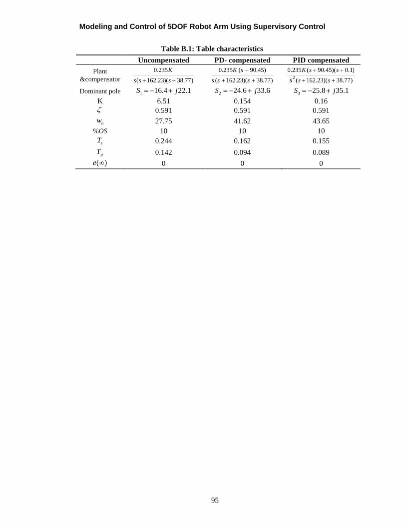
Modeling and Control of 5DOF Robot Arm Using Supervisory Control
95
Table B.1: Table characteristics
Uncompensated PD- compensated PID compensated
Plant &compensator
0.235
( 162.23)( 38.77)
K
s s s
0.235 ( 90.45)
( 162.23)( 38.77)
K s
s s s
2
0.235 ( 90.45)( 0.1)
( 162.23)( 38.77)
K s s
s ss
Dominant pole 1 16.4 22.1S j 2 24.6 33.6S j 3 25.8 35.1S j
K 6.51 0.154 0.16 0.591 0.591 0.591
nw 27.75 41.62 43.65 %OS 10 10 10
sT 0.244 0.162 0.155
pT 0.142 0.094 0.089 ( )e 0 0 0
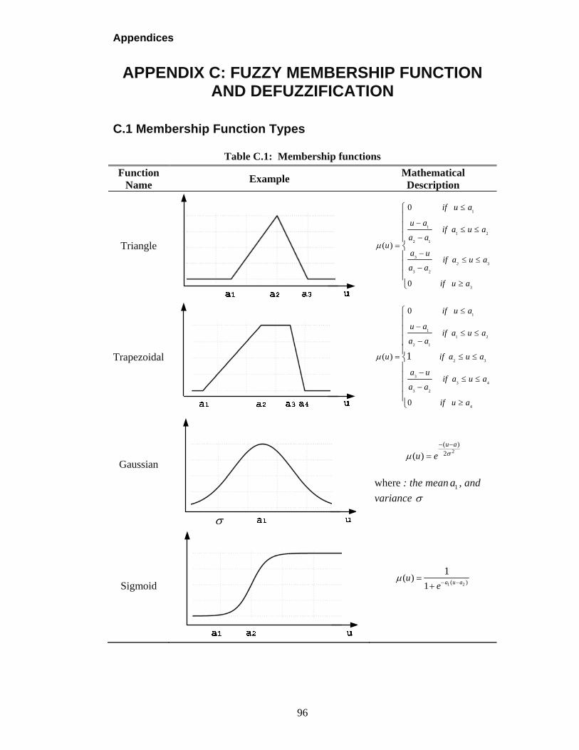
Appendices
96
APPENDIX C: FUZZY MEMBERSHIP FUNCTION AND DEFUZZIFICATION
C.1 Membership Function Types
Table C.1: Membership functions
Function Name Example
Mathematical Description
Triangle
1
1
1 2
2 1
3
2 3
3 2
3
0
( )
0
if u a
u aif a u a
a au
a uif a u a
a a
if u a
Trapezoidal
1
1
1 2
2 1
2 3
3
3 4
3 2
4
0
( )
0
1
if u a
u aif a u a
a a
u if a u a
a uif a u a
a a
if u a
Gaussian
2( )2( )u a
u e
where : the mean 1a , and
variance
Sigmoid 1 2( )( )
1
1a u a
ue
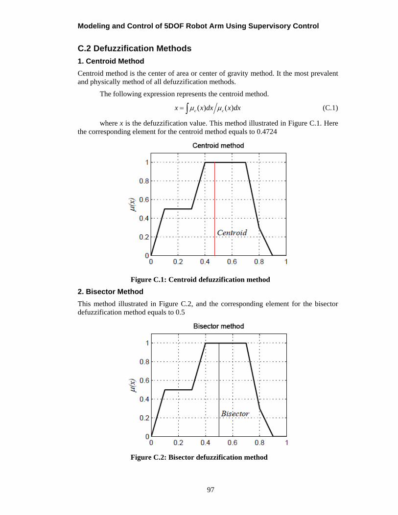
Modeling and Control of 5DOF Robot Arm Using Supervisory Control
97
C.2 Defuzzification Methods
1. Centroid Method
Centroid method is the center of area or center of gravity method. It the most prevalent and physically method of all defuzzification methods.
The following expression represents the centroid method.
( ) ( )c cx x dx x dx (C.1)
where x is the defuzzification value. This method illustrated in Figure C.1. Here the corresponding element for the centroid method equals to 0.4724
Figure C.1: Centroid defuzzification method
2. Bisector Method
This method illustrated in Figure C.2, and the corresponding element for the bisector defuzzification method equals to 0.5
Figure C.2: Bisector defuzzification method
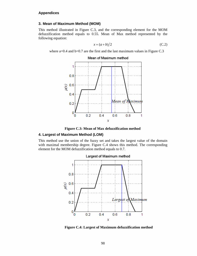
Appendices
98
3. Mean of Maximum Method (MOM)
This method illustrated in Figure C.3, and the corresponding element for the MOM defuzzification method equals to 0.55. Mean of Max method represented by the following equation:
( ) 2x a b (C.2)
where a=0.4 and b=0.7 are the first and the last maximum values in Figure C.3
Figure C.3: Mean of Max defuzzification method
4. Largest of Maximum Method (LOM)
This method use the union of the fuzzy set and takes the largest value of the domain with maximal membership degree. Figure C.4 shows this method. The corresponding element for the MOM defuzzification method equals to 0.7.
Figure C.4: Largest of Maximum defuzzification method
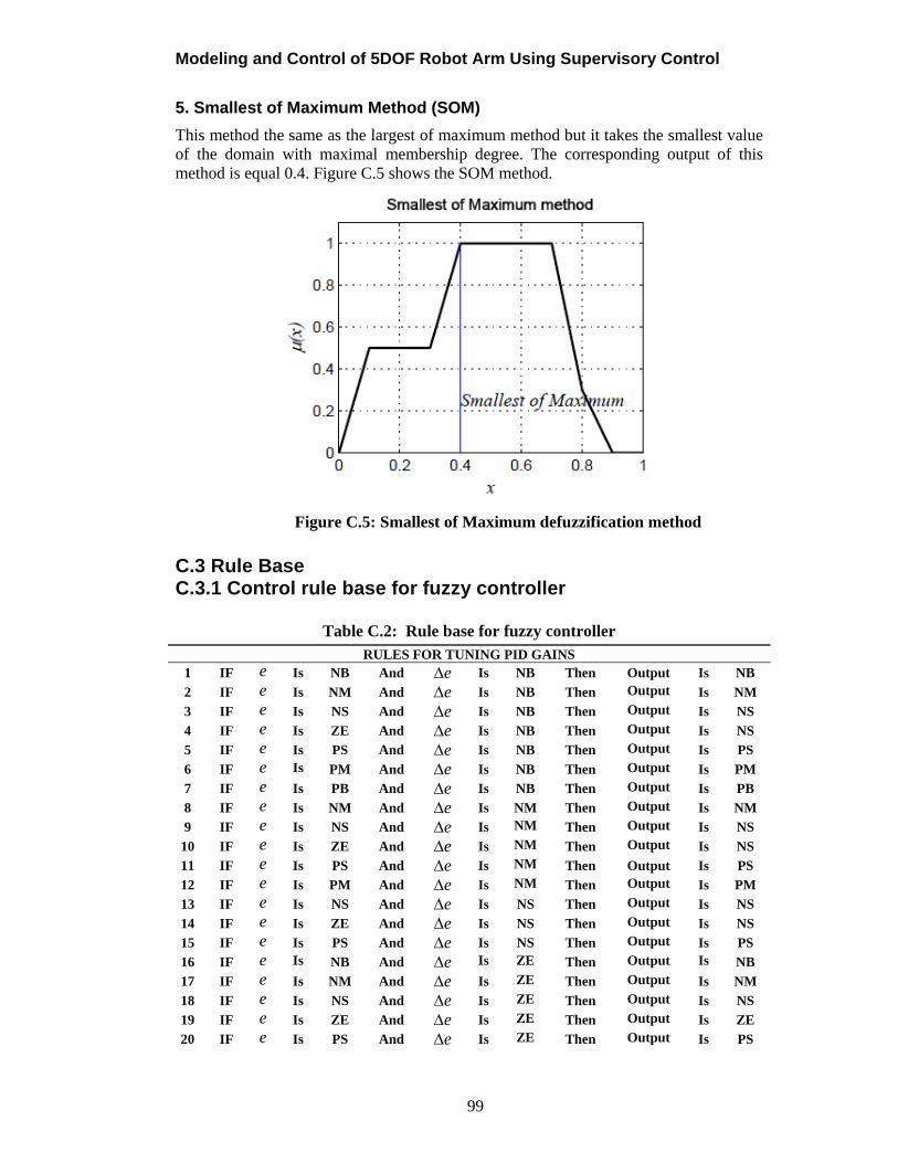
Modeling and Control of 5DOF Robot Arm Using Supervisory Control
99
5. Smallest of Maximum Method (SOM)
This method the same as the largest of maximum method but it takes the smallest value of the domain with maximal membership degree. The corresponding output of this method is equal 0.4. Figure C.5 shows the SOM method.
Figure C.5: Smallest of Maximum defuzzification method
C.3 Rule Base C.3.1 Control rule base for fuzzy controller
Table C.2: Rule base for fuzzy controller RULES FOR TUNING PID GAINS
1 IF e Is NB And e Is NB Then Output Is NB
2 IF e Is NM And e Is NB Then Output Is NM
3 IF e Is NS And e Is NB Then Output Is NS
4 IF e Is ZE And e Is NB Then Output Is NS
5 IF e Is PS And e Is NB Then Output Is PS
6 IF e Is PM And e Is NB Then Output Is PM
7 IF e Is PB And e Is NB Then Output Is PB
8 IF e Is NM And e Is NM Then Output Is NM
9 IF e Is NS And e Is NM Then Output Is NS
10 IF e Is ZE And e Is NM Then Output Is NS
11 IF e Is PS And e Is NM Then Output Is PS
12 IF e Is PM And e Is NM Then Output Is PM
13 IF e Is NS And e Is NS Then Output Is NS
14 IF e Is ZE And e Is NS Then Output Is NS
15 IF e Is PS And e Is NS Then Output Is PS
16 IF e Is NB And e Is ZE Then Output Is NB
17 IF e Is NM And e Is ZE Then Output Is NM
18 IF e Is NS And e Is ZE Then Output Is NS
19 IF e Is ZE And e Is ZE Then Output Is ZE
20 IF e Is PS And e Is ZE Then Output Is PS
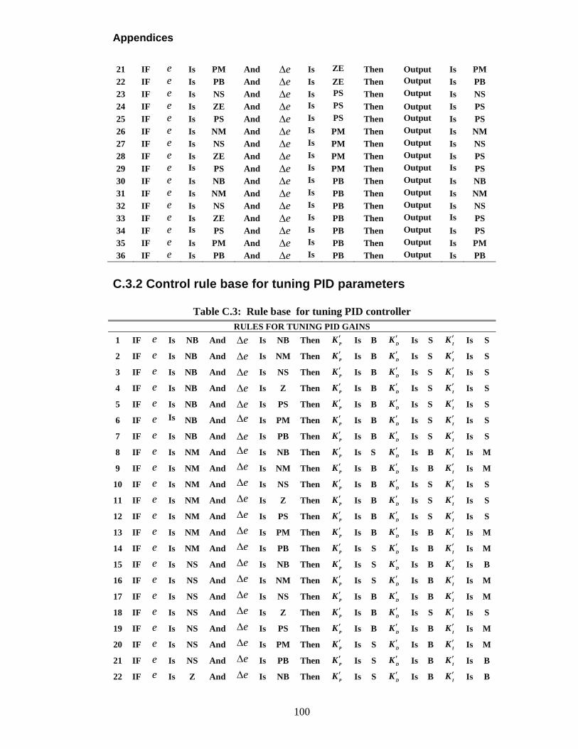
Appendices
100
21 IF e Is PM And e Is ZE Then Output Is PM
22 IF e Is PB And e Is ZE Then Output Is PB
23 IF e Is NS And e Is PS Then Output Is NS
24 IF e Is ZE And e Is PS Then Output Is PS
25 IF e Is PS And e Is PS Then Output Is PS
26 IF e Is NM And e Is PM Then Output Is NM
27 IF e Is NS And e Is PM Then Output Is NS
28 IF e Is ZE And e Is PM Then Output Is PS
29 IF e Is PS And e Is PM Then Output Is PS
30 IF e Is NB And e Is PB Then Output Is NB
31 IF e Is NM And e Is PB Then Output Is NM
32 IF e Is NS And e Is PB Then Output Is NS
33 IF e Is ZE And e Is PB Then Output Is PS
34 IF e Is PS And e Is PB Then Output Is PS
35 IF e Is PM And e Is PB Then Output Is PM
36 IF e Is PB And e Is PB Then Output Is PB
C.3.2 Control rule base for tuning PID parameters
Table C.3: Rule base for tuning PID controller RULES FOR TUNING PID GAINS
1 IF e Is NB And e Is NB Then P
K Is B D
K Is S I
K Is S
2 IF e Is NB And e Is NM Then P
K Is B D
K Is S I
K Is S
3 IF e Is NB And e Is NS Then P
K Is B D
K Is S I
K Is S
4 IF e Is NB And e Is Z Then P
K Is B D
K Is S I
K Is S
5 IF e Is NB And e Is PS Then P
K Is B D
K Is S I
K Is S
6 IF e Is NB And e Is PM Then P
K Is B D
K Is S I
K Is S
7 IF e Is NB And e Is PB Then P
K Is B D
K Is S I
K Is S
8 IF e Is NM And e Is NB Then P
K Is S D
K Is B I
K Is M
9 IF e Is NM And e Is NM Then P
K Is B D
K Is B I
K Is M
10 IF e Is NM And e Is NS Then P
K Is B D
K Is S I
K Is S
11 IF e Is NM And e Is Z Then P
K Is B D
K Is S I
K Is S
12 IF e Is NM And e Is PS Then P
K Is B D
K Is S I
K Is S
13 IF e Is NM And e Is PM Then P
K Is B D
K Is B I
K Is M
14 IF e Is NM And e Is PB Then P
K Is S D
K Is B I
K Is M
15 IF e Is NS And e Is NB Then P
K Is S D
K Is B I
K Is B
16 IF e Is NS And e Is NM Then P
K Is S D
K Is B I
K Is M
17 IF e Is NS And e Is NS Then P
K Is B D
K Is B I
K Is M
18 IF e Is NS And e Is Z Then P
K Is B D
K Is S I
K Is S
19 IF e Is NS And e Is PS Then P
K Is B D
K Is B I
K Is M
20 IF e Is NS And e Is PM Then P
K Is S D
K Is B I
K Is M
21 IF e Is NS And e Is PB Then P
K Is S D
K Is B I
K Is B
22 IF e Is Z And e Is NB Then P
K Is S D
K Is B I
K Is B
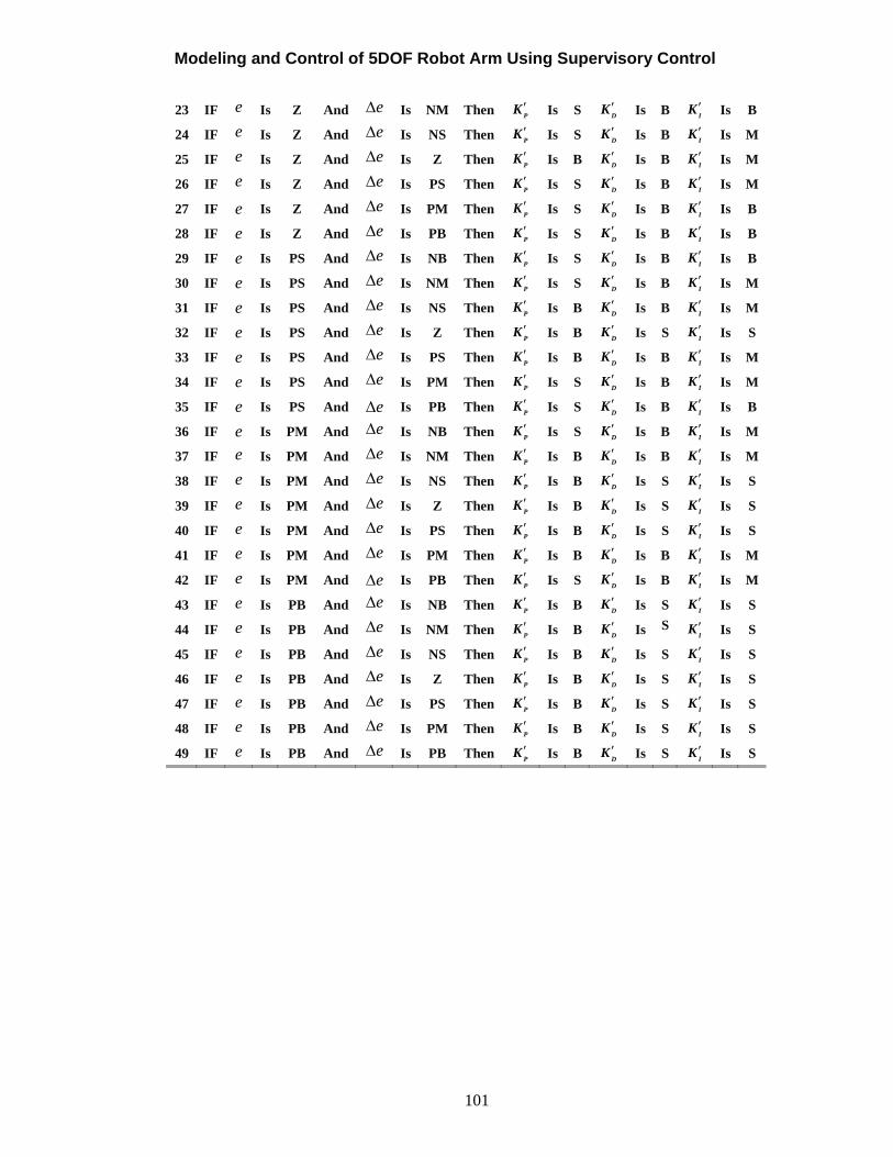
Modeling and Control of 5DOF Robot Arm Using Supervisory Control
101
23 IF e Is Z And e Is NM Then P
K Is S D
K Is B I
K Is B
24 IF e Is Z And e Is NS Then P
K Is S D
K Is B I
K Is M
25 IF e Is Z And e Is Z Then P
K Is B D
K Is B I
K Is M
26 IF e Is Z And e Is PS Then P
K Is S D
K Is B I
K Is M
27 IF e Is Z And e Is PM Then P
K Is S D
K Is B I
K Is B
28 IF e Is Z And e Is PB Then P
K Is S D
K Is B I
K Is B
29 IF e Is PS And e Is NB Then P
K Is S D
K Is B I
K Is B
30 IF e Is PS And e Is NM Then P
K Is S D
K Is B I
K Is M
31 IF e Is PS And e Is NS Then P
K Is B D
K Is B I
K Is M
32 IF e Is PS And e Is Z Then P
K Is B D
K Is S I
K Is S
33 IF e Is PS And e Is PS Then P
K Is B D
K Is B I
K Is M
34 IF e Is PS And e Is PM Then P
K Is S D
K Is B I
K Is M
35 IF e Is PS And e Is PB Then P
K Is S D
K Is B I
K Is B
36 IF e Is PM And e Is NB Then P
K Is S D
K Is B I
K Is M
37 IF e Is PM And e Is NM Then P
K Is B D
K Is B I
K Is M
38 IF e Is PM And e Is NS Then P
K Is B D
K Is S I
K Is S
39 IF e Is PM And e Is Z Then P
K Is B D
K Is S I
K Is S
40 IF e Is PM And e Is PS Then P
K Is B D
K Is S I
K Is S
41 IF e Is PM And e Is PM Then P
K Is B D
K Is B I
K Is M
42 IF e Is PM And e Is PB Then P
K Is S D
K Is B I
K Is M
43 IF e Is PB And e Is NB Then P
K Is B D
K Is S I
K Is S
44 IF e Is PB And e Is NM Then P
K Is B D
K Is S I
K Is S
45 IF e Is PB And e Is NS Then P
K Is B D
K Is S I
K Is S
46 IF e Is PB And e Is Z Then P
K Is B D
K Is S I
K Is S
47 IF e Is PB And e Is PS Then P
K Is B D
K Is S I
K Is S
48 IF e Is PB And e Is PM Then P
K Is B D
K Is S I
K Is S
49 IF e Is PB And e Is PB Then P
K Is B D
K Is S I
K Is S
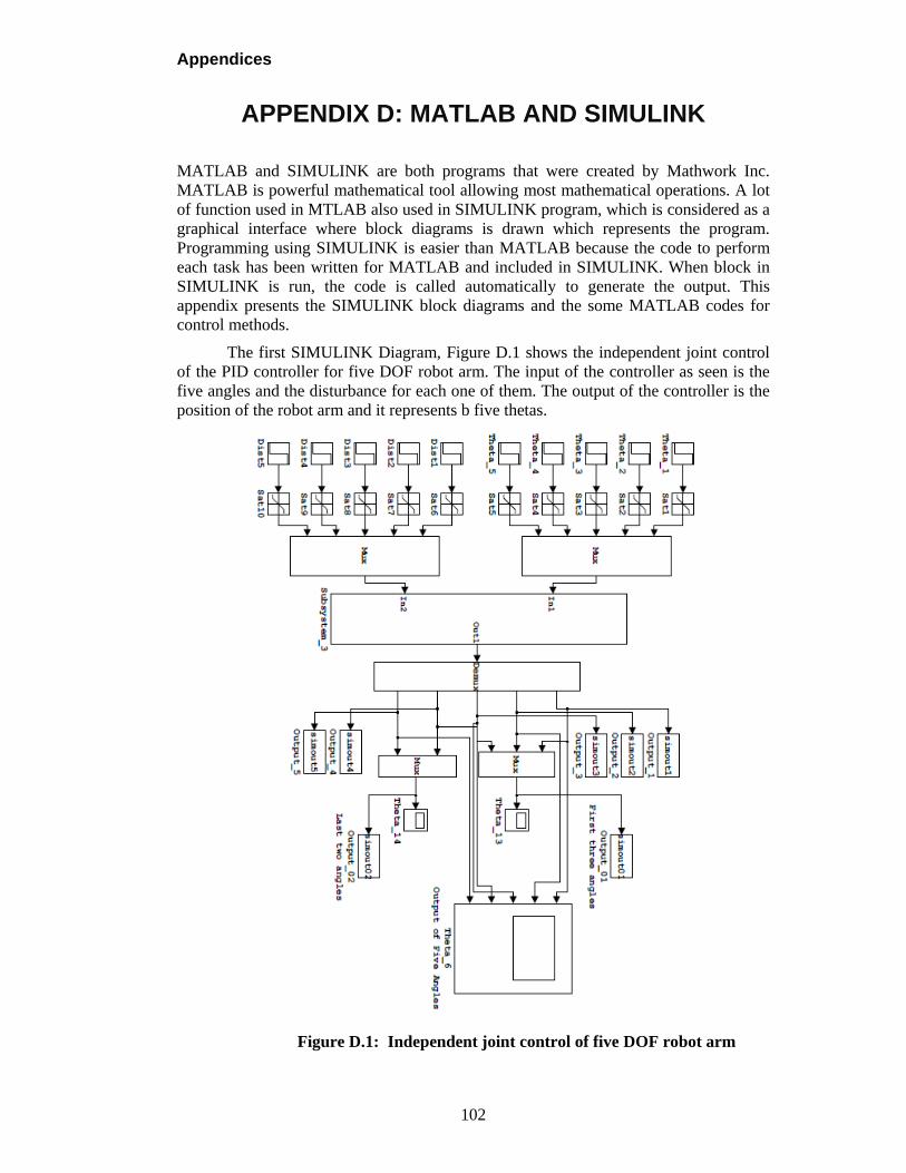
Appendices
102
APPENDIX D: MATLAB AND SIMULINK
MATLAB and SIMULINK are both programs that were created by Mathwork Inc. MATLAB is powerful mathematical tool allowing most mathematical operations. A lot of function used in MTLAB also used in SIMULINK program, which is considered as a graphical interface where block diagrams is drawn which represents the program. Programming using SIMULINK is easier than MATLAB because the code to perform each task has been written for MATLAB and included in SIMULINK. When block in SIMULINK is run, the code is called automatically to generate the output. This appendix presents the SIMULINK block diagrams and the some MATLAB codes for control methods.
The first SIMULINK Diagram, Figure D.1 shows the independent joint control of the PID controller for five DOF robot arm. The input of the controller as seen is the five angles and the disturbance for each one of them. The output of the controller is the position of the robot arm and it represents b five thetas.
Figure D.1: Independent joint control of five DOF robot arm
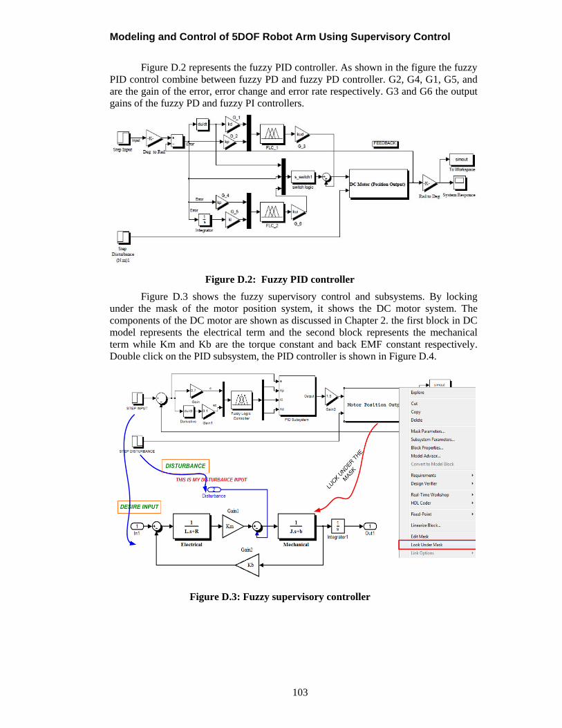
Modeling and Control of 5DOF Robot Arm Using Supervisory Control
103
Figure D.2 represents the fuzzy PID controller. As shown in the figure the fuzzy PID control combine between fuzzy PD and fuzzy PD controller. G2, G4, G1, G5, and are the gain of the error, error change and error rate respectively. G3 and G6 the output gains of the fuzzy PD and fuzzy PI controllers.
Figure D.2: Fuzzy PID controller
Figure D.3 shows the fuzzy supervisory control and subsystems. By locking under the mask of the motor position system, it shows the DC motor system. The components of the DC motor are shown as discussed in Chapter 2. the first block in DC model represents the electrical term and the second block represents the mechanical term while Km and Kb are the torque constant and back EMF constant respectively. Double click on the PID subsystem, the PID controller is shown in Figure D.4.
Figure D.3: Fuzzy supervisory controller
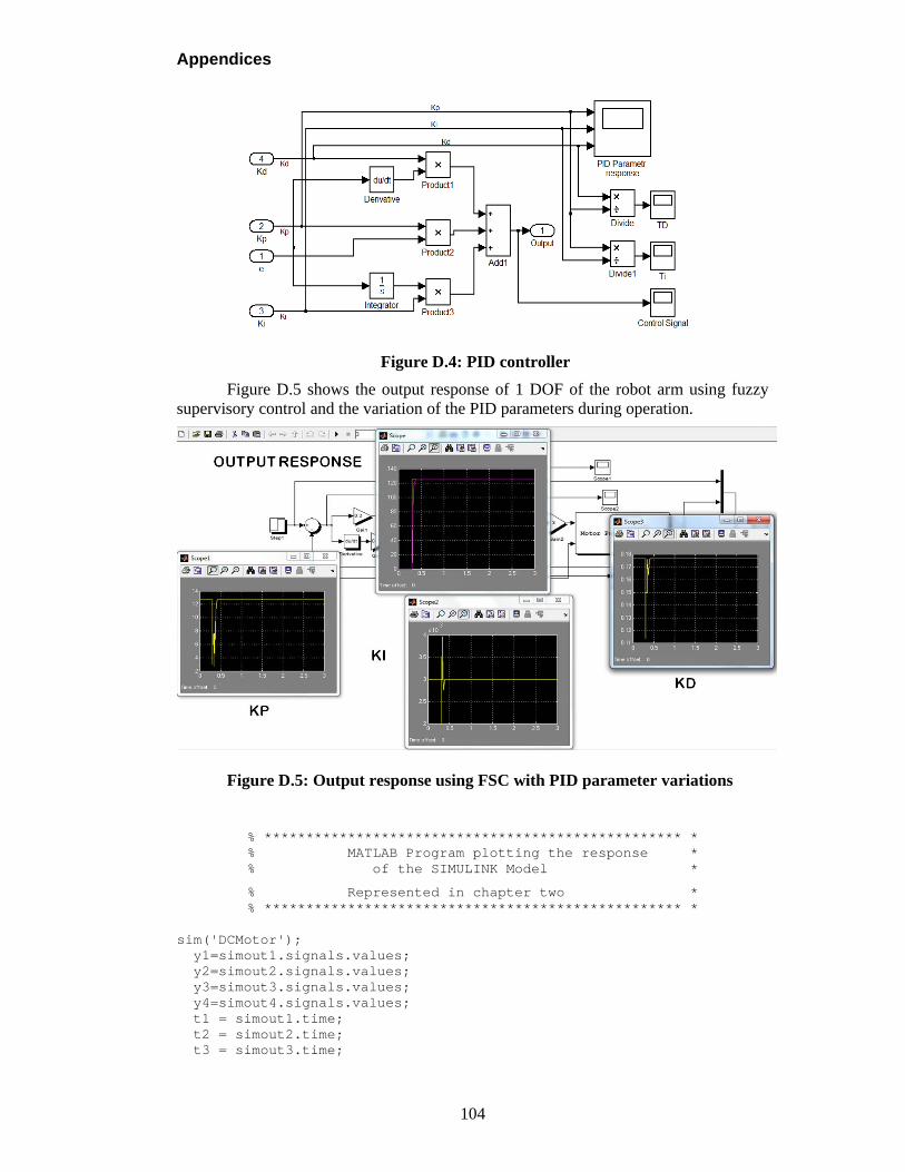
Appendices
104
Figure D.4: PID controller
Figure D.5 shows the output response of 1 DOF of the robot arm using fuzzy supervisory control and the variation of the PID parameters during operation.
Figure D.5: Output response using FSC with PID parameter variations
% ************************************************** * % MATLAB Program plotting the response * % of the SIMULINK Model *
% Represented in chapter two * % ************************************************** *
sim('DCMotor'); y1=simout1.signals.values; y2=simout2.signals.values; y3=simout3.signals.values; y4=simout4.signals.values; t1 = simout1.time; t2 = simout2.time; t3 = simout3.time;
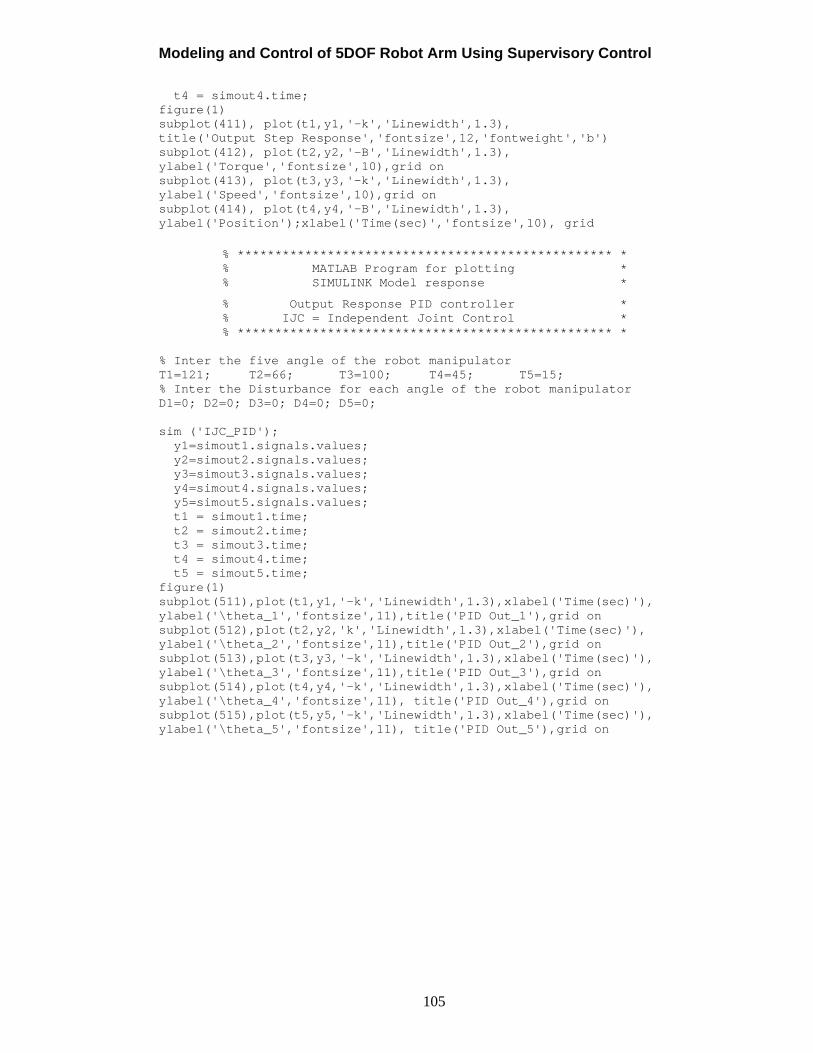
Modeling and Control of 5DOF Robot Arm Using Supervisory Control
105
t4 = simout4.time; figure(1) subplot(411), plot(t1,y1,'-k','Linewidth',1.3), title('Output Step Response','fontsize',12,'fontweight','b') subplot(412), plot(t2,y2,'-B','Linewidth',1.3), ylabel('Torque','fontsize',10),grid on subplot(413), plot(t3,y3,'-k','Linewidth',1.3), ylabel('Speed','fontsize',10),grid on subplot(414), plot(t4,y4,'-B','Linewidth',1.3), ylabel('Position');xlabel('Time(sec)','fontsize',10), grid
% ************************************************** * % MATLAB Program for plotting * % SIMULINK Model response *
% Output Response PID controller * % IJC = Independent Joint Control * % ************************************************** *
% Inter the five angle of the robot manipulator T1=121; T2=66; T3=100; T4=45; T5=15; % Inter the Disturbance for each angle of the robot manipulator D1=0; D2=0; D3=0; D4=0; D5=0; sim ('IJC_PID'); y1=simout1.signals.values; y2=simout2.signals.values; y3=simout3.signals.values; y4=simout4.signals.values; y5=simout5.signals.values; t1 = simout1.time; t2 = simout2.time; t3 = simout3.time; t4 = simout4.time; t5 = simout5.time; figure(1) subplot(511),plot(t1,y1,'-k','Linewidth',1.3),xlabel('Time(sec)'), ylabel('\theta_1','fontsize',11),title('PID Out_1'),grid on subplot(512),plot(t2,y2,'k','Linewidth',1.3),xlabel('Time(sec)'), ylabel('\theta_2','fontsize',11),title('PID Out_2'),grid on subplot(513),plot(t3,y3,'-k','Linewidth',1.3),xlabel('Time(sec)'), ylabel('\theta_3','fontsize',11),title('PID Out_3'),grid on subplot(514),plot(t4,y4,'-k','Linewidth',1.3),xlabel('Time(sec)'), ylabel('\theta_4','fontsize',11), title('PID Out_4'),grid on subplot(515),plot(t5,y5,'-k','Linewidth',1.3),xlabel('Time(sec)'), ylabel('\theta_5','fontsize',11), title('PID Out_5'),grid on