Embed Size (px)
Citation preview
Atmos. Chem. Phys., 15, 11753–11772, 2015
www.atmos-chem-phys.net/15/11753/2015/
doi:10.5194/acp-15-11753-2015
© Author(s) 2015. CC Attribution 3.0 License.
Modelling marine emissions and atmospheric distributions of
halocarbons and dimethyl sulfide: the influence of prescribed water
concentration vs. prescribed emissions
S. T. Lennartz1, G. Krysztofiak2,a, C. A. Marandino1, B.-M. Sinnhuber2, S. Tegtmeier1, F. Ziska1, R. Hossaini3,
K. Krüger4, S. A. Montzka5, E. Atlas6, D. E. Oram7, T. Keber8, H. Bönisch8, and B. Quack1
1GEOMAR Helmholtz-Centre for Ocean Research Kiel, Kiel, Germany2Karlsruhe Institute of Technology, Institute for Meteorology and Climate Research, Karlsruhe, Germany3School of Earth and Environment, University of Leeds, Leeds, UK4University of Oslo, Department of Geosciences, Oslo, Norway5NOAA/CMDL, Boulder, CO, USA6RSMAS/MAC, University of Miami, Florida, USA7National Centre for Atmospheric Science, Centre for Oceanography and Atmospheric Science,
University of East Anglia, Norwich, UK8Goethe University Frankfurt a. M., Institute for Atmospheric and Environmental Sciences, Frankfurt, Germanyanow at: LPC2E, UMR 7328, CNRS-Université d’Orléans, 45071 Orléans CEDEX 2, France
Correspondence to: S. T. Lennartz ([email protected])
Received: 24 April 2015 – Published in Atmos. Chem. Phys. Discuss.: 30 June 2015
Revised: 23 September 2015 – Accepted: 30 September 2015 – Published: 22 October 2015
Abstract. Marine-produced short-lived trace gases such as
dibromomethane (CH2Br2), bromoform (CHBr3), methylio-
dide (CH3I) and dimethyl sulfide (DMS) significantly im-
pact tropospheric and stratospheric chemistry. Describing
their marine emissions in atmospheric chemistry models as
accurately as possible is necessary to quantify their im-
pact on ozone depletion and Earth’s radiative budget. So
far, marine emissions of trace gases have mainly been pre-
scribed from emission climatologies, thus lacking the inter-
action between the actual state of the atmosphere and the
ocean. Here we present simulations with the chemistry cli-
mate model EMAC (ECHAM5/MESSy Atmospheric Chem-
istry) with online calculation of emissions based on surface
water concentrations, in contrast to directly prescribed emis-
sions. Considering the actual state of the model atmosphere
results in a concentration gradient consistent with model real-
time conditions at the ocean surface and in the atmosphere,
which determine the direction and magnitude of the com-
puted flux. This method has a number of conceptual and
practical benefits, as the modelled emission can respond con-
sistently to changes in sea surface temperature, surface wind
speed, sea ice cover and especially atmospheric mixing ra-
tio. This online calculation could enhance, dampen or even
invert the fluxes (i.e. deposition instead of emissions) of very
short-lived substances (VSLS). We show that differences be-
tween prescribing emissions and prescribing concentrations
(−28 % for CH2Br2 to+11 % for CHBr3) result mainly from
consideration of the actual, time-varying state of the atmo-
sphere. The absolute magnitude of the differences depends
mainly on the surface ocean saturation of each particular gas.
Comparison to observations from aircraft, ships and ground
stations reveals that computing the air–sea flux interactively
leads in most of the cases to more accurate atmospheric mix-
ing ratios in the model compared to the computation from
prescribed emissions. Calculating emissions online also en-
ables effective testing of different air–sea transfer velocity
(k) parameterizations, which was performed here for eight
different parameterizations. The testing of these different k
values is of special interest for DMS, as recently published
parameterizations derived by direct flux measurements using
eddy covariance measurements suggest decreasing k values
at high wind speeds or a linear relationship with wind speed.
Published by Copernicus Publications on behalf of the European Geosciences Union.
11754 S. T. Lennartz et al.: Modelling marine emissions and atmospheric distributions
Implementing these parameterizations reduces discrepancies
in modelled DMS atmospheric mixing ratios and observa-
tions by a factor of 1.5 compared to parameterizations with a
quadratic or cubic relationship to wind speed.
1 Introduction
The oceans emit large amounts of halogen- (Penkett et al.,
1985; Quack and Wallace, 2003) and sulfur-containing sub-
stances (Bates et al., 1992; Watts, 2000) that influence atmo-
spheric chemistry. Organic bromine and iodine in the atmo-
sphere is largely supplied by oceanic emissions of very short-
lived substances (VSLS) such as dibromomethane (CH2Br2),
bromoform (CHBr3) and methyliodide (CH3I) (Lovelock
and Maggs, 1973; Hossaini et al., 2013). Also, a large frac-
tion of the atmospheric sulfur loading is due to oceanic
emissions of OCS, CS2, H2S and dimethyl sulfide (DMS;
CH3SCH3), the latter being the major compound transport-
ing sulfur from the ocean to the atmosphere (Watts, 2000;
Sheng et al., 2015). Thus, we focus on DMS in this study.
Assessing marine emissions of VSLS is crucial, as they
significantly influence Earth’s atmosphere in both the tro-
posphere and the stratosphere. In the troposphere, bromine-
containing VSLS such as CHBr3 and CH2Br2 contribute
to ozone destruction and alter the oxidative capacity (von
Glasow et al., 2004; Salawitch, 2006). Oceanic CH3I is the
main organic iodine compound in the atmosphere (Lovelock
and Maggs, 1973) and impacts tropospheric oxidative ca-
pacity and ozone destruction (Chameides and Davis, 1980;
Saiz-Lopez et al., 2012). Iodine oxides, which can be prod-
uct gases of CH3I are likely to contribute to nucleation and
growth of secondary marine aerosol production (O’Dowd
and De Leeuw, 2007). DMS emitted to the troposphere is
a precursor of secondary organic aerosol and potentially
cloud condensation nuclei and thus influences the radiative
budget (Charlson et al., 1987). Halogenated VSLS also en-
hance stratospheric ozone depletion (Sinnhuber and Meul,
2015) and thus contribute to the ozone-driven radiative forc-
ing of climate (Hossaini et al., 2015). Despite the short life-
time of CH3I (4–7 days) compared to the bromocarbons (6–
120 days), there is potential for a small fraction of marine-
produced CH3I to be transported to the stratosphere where
it also contributes to ozone depletion (Tegtmeier et al., 2013;
Solomon et al., 1994). DMS has a shorter lifetime of 11 min–
46 h (Barnes et al., 2006; Osthoff et al., 2009) compared
to CH3I. Despite the short lifetime, there is potential even
for the very short-lived DMS to be transported to the trop-
ical tropopause layer (TTL) in convective hot spot regions
(Marandino et al., 2013a, b).
The impact of marine VSLS emissions on atmospheric
chemistry has been studied in chemistry–climate and trans-
port models (e.g. Salawitch et al., 2005; Kerkweg et al.,
2006b; Sinnhuber et al., 2009; Liang et al., 2010; Ordóñez
et al., 2012). Therein, marine emissions of the VSLS have
mainly been based on prescribed boundary layer mixing ra-
tios (Aschmann et al., 2009) or emission scenarios (Warwick
et al., 2006; Liang et al., 2010; Ordóñez et al., 2012; Hossaini
et al., 2013). However, prescribing emissions in atmospheric
models lacks the impact of the atmospheric boundary layer
mixing ratio on the concentration gradient. This concentra-
tion gradient at the interface between ocean and atmosphere
directly influences the emissions, as it determines the direc-
tion and magnitude of the flux. The lack of potential feed-
backs can result in a modelled atmospheric surface concen-
tration inconsistent with the oceanic surface concentration.
Here, we evaluate a conceptually different way of consid-
ering marine emissions in chemical climate models that is
based on a consistent concentration gradient between ocean
and atmosphere. In contrast to previous approaches of ei-
ther specifying atmospheric surface mixing ratios or speci-
fying sea-to-air fluxes, water concentrations are prescribed
and emissions are calculated online. Thus, the concentra-
tion gradient at the interface and the emissions are consis-
tent with the atmospheric boundary layer and the ocean sur-
face, and the emissions can respond to the actual state of
the atmosphere. The approach is applied to established con-
centration climatologies of short-lived halocarbons (CH2Br2,
CHBr3, CH3I) and sulfur compounds (DMS) that share com-
mon characteristics such as supersaturation in the surface
ocean and marine production. For the halocarbons, this set-
up is applied for the first time and uses surface ocean con-
centration climatologies derived from observations by Ziska
et al. (2013). Oceanic DMS emissions have been evaluated
in coupled ocean–atmosphere models (Kloster et al., 2006;
Cameron-Smith et al., 2011) or modelled online during a test
for the implementation of different submodels (Kerkweg et
al., 2006b). In our study, the focus lies on how to consider
oceanic emissions in a stand-alone atmospheric model, and
uses the most updated DMS concentrations available (Lana
et al., 2011). Additionally, we compare the output of the two
methods with observations from aircraft and ship campaigns.
Prescribing water concentrations and calculating emis-
sions online enables convenient testing of different air–sea
gas exchange parameterizations. Air–sea gas exchange is cal-
culated as the product of the concentration gradient between
air and water at the surface and the transfer velocity. The lat-
ter needs to be parameterized, and many different parameteri-
zations have been published (see e.g. Wanninkhof et al., 2009
for a summary). Most parameterizations relate the transfer
velocity to wind speed (e.g. Liss and Merlivat, 1986; Wan-
ninkhof and McGillis, 1999; Nightingale et al., 2000; Ho et
al., 2006), but others take the effect of bubble-mediated trans-
fer (Asher and Wanninkhof, 1998) or enhancement by rain
(Ho et al., 1997, 2004) into account. Testing a variety of dif-
ferent parameterizations on prescribed water concentrations
to calculate atmospheric abundances provides information on
the uncertainties of global emission estimates.
The experimental set-up consists of two steps. First, we
prescribed surface water concentrations in the chemistry cli-
Atmos. Chem. Phys., 15, 11753–11772, 2015 www.atmos-chem-phys.net/15/11753/2015/

S. T. Lennartz et al.: Modelling marine emissions and atmospheric distributions 11755
mate model EMAC (ECHAM5/MESSy Atmospheric Chem-
istry) (Jöckel et al., 2006, 2010) and air–sea exchange of
VSLS was then calculated online by the submodel AIRSEA
(Pozzer et al., 2006). The model results are then evaluated
and compared to a simulation where the difference results
from prescribed VSLS emissions (PE). To compare the sim-
ulation set-up with prescribed emissions to the set-up with
prescribed water concentrations, we used the same concen-
tration climatologies that were used to create the emission
climatologies. In our study, these concentration and corre-
sponding emission climatologies were published by Ziska
et al. (2013) for the halocarbons and Lana et al. (2011) for
DMS. The modelled atmospheric mixing ratios of the gases
are compared to measurements from time series of ground-
based stations, ship and aircraft campaigns in order to iden-
tify whether the online calculation is simulating the atmo-
spheric mixing ratios more accurately. In a second step, we
use the coupled module to test the sensitivity of the global
emissions to eight different, frequently used or recently pub-
lished, transfer velocity parameterizations.
2 Model set-up and data description
2.1 The atmosphere-chemistry model EMAC
The EMAC model is a global atmospheric chemistry
climate model described in Jöckel et al. (2006, 2010).
ECHAM5/MESSy includes submodels describing processes
of the troposphere and middle atmosphere as well as interac-
tion with land and human influences. Air–sea gas exchange
is calculated in EMAC with the submodule AIRSEA, as de-
scribed by Pozzer et al. (2006).
The numerical simulations were nudged towards the
European Centre for Medium-Range Weather Forecasts
(ECMWF) ERA-Interim reanalysis (Dee et al., 2011) every
6 h (temperature, divergence, vorticity, surface pressure). The
resolution of the EMAC atmosphere was∼ 2.8◦× 2.8◦ (T42)
and 39 vertical hybrid pressure levels up to 0.01 hPa (L39).
The effect of resolution on the results tested with a finer res-
olution (T106) was only minor (see Table S2 in the Sup-
plement). The atmospheric model as well as the submodel
AIRSEA uses a time step of 600 s. The convective transport
follows the scheme of Tiedtke (1989) and the tracer advec-
tion is described in Lin and Rood (1996). An overview of
these nudged simulation set-ups can be found in Sect. 2.3.
The simulations include the four very short-lived species,
CH2Br2, CHBr3, CH3I and DMS, and simplified atmo-
spheric loss reactions for them. The loss reactions include
– oxidation with OH, O(1D), Cl and photolysis for CHBr3
and CH2Br2 following the reactions rates by Sander et
al. (2011);
– oxidation with OH, Cl and photolysis for CH3I (Sander
et al., 2011);
– and oxidation with OH and O(3P) for DMS (Sander et
al., 2011).
EMAC uses monthly mean concentrations of OH, devel-
oped and evaluated for the TransCom-CH4 model intercom-
parison project, and discussed in detail by Patra et al. (2014).
Monthly mean photolysis rates for VSLS were calculated by
the TOMCAT CTM (chemical transport model) which has
been used extensively to examine the tropospheric chem-
istry of VSLS (e.g. Hossaini et al., 2013). These fields
were provided at a horizontal resolution of 2.8◦× 2.8◦
(longitude× latitude) and on 60 vertical levels (surface to
∼ 60 km). TOMCAT calculates photolysis rates online us-
ing the code of Hough (1988) which considers both di-
rect and scattered radiation. Within TOMCAT, this scheme
is supplied with surface albedo, monthly mean climatolog-
ical cloud fields and ozone and temperature profiles. The
photolysis rates have recently been used and evaluated as
part of the ongoing TransCom-VSLS model intercomparison
project (http://www.transcom-vsls.com).
The simulated atmospheric lifetimes in our set-up gener-
ally agree well with published estimates for these gases, indi-
cating that the basic assumption of the simplified chemistry
applied here is valid. The local mean tropical (20◦ N–20◦ S)
lifetime of CH2Br2 in the troposphere in our model study is
143 days and thus lies below 167 days, which was found in
Hossaini et al. (2010). The mean tropospheric tropical life-
time of CHBr3 is 20 days in our study, which is consistent
within 10 % with a recent reevaluation of CHBr3 lifetime by
Papanastasiou et al. (2014), together with a recent reevalua-
tion of the reaction of OH with CHBr3 by Orkin et al. (2013).
The local lifetime of CH3I in our study is 3 days, which is in
accordance with the study of Tegtmeier et al. (2013). The
tropical lifetime of DMS in our study ranges between less
than 1 day and up to 3 days and is thus within but at the
higher end of the range of 11 min–46 h (Barnes et al., 2006;
Osthoff et al., 2009).
2.2 Parameterizations of air-sea gas exchange
In this study, the AIRSEA submodel (Pozzer et al., 2006) and
its approach for air–sea gas exchange was adopted, using the
two-layer model (Liss and Slater, 1974). Marine emissions
(F ) of gases are calculated as the product of the concentra-
tion gradient between air and water concentration of the gas
(1c) and the transfer velocity (k; Eq. 1), which needs to be
parameterized.
F = k ·1c = k · (cw−H · cair) (1)
with cw being the water concentration, H the Henry constant
(dimensionless, water over air) and cair the concentration of
the gas in air which was taken from the modelled atmosphere
in the respective time step. Henry constants and their temper-
ature dependencies are taken from Moore et al. (1995) for the
halocarbons and De Bruyn et al. (1995) for DMS.
www.atmos-chem-phys.net/15/11753/2015/ Atmos. Chem. Phys., 15, 11753–11772, 2015
11756 S. T. Lennartz et al.: Modelling marine emissions and atmospheric distributions
The transfer velocity k comprises air- (kair) and water-side
(kw) transfer velocities (Eq. 2) in all parameterizations with
the Henry constant (H ), air temperature (Tair) and the ideal
gas constant (R):
k =
(1
kw
+R ·H · Tair
kair
)−1
. (2)
The water-side transfer velocity kw is often parameterized
in relation to wind speed with linear (e.g. Liss and Merli-
vat, 1986), quadratic (e.g. Ho et al., 2006) or cubic (e.g.
Wanninkhof and McGillis, 1999) dependencies. Differences
between these parameterizations arise from different tech-
niques to determine kw. The kw parameterizations tested in
our study result from tracer release experiments in wind
tanks (Liss and Merlivat, 1986), from deliberate tracer tech-
niques in the open ocean (Nightingale et al., 2001; Ho et al.,
2006) or from direct flux measurements using eddy covari-
ance (Wanninkhof et al., 1999; Marandino et al., 2009; Bell
et al., 2013). Additional drivers of gas exchange, e.g. bubble-
mediated transfer (e.g. Asher and Wanninkhof, 1998) and en-
hancement in the presence of rain (e.g. Ho et al., 2004) are
discussed. Bubble-mediated transfer has been suggested to
be influential for gases with low solubilities since they more
quickly escape from the liquid phase into the bubbles. Asher
and Wanninkhof (1998) reanalysed data from a dual tracer
experiment and found a better fit when bubble-mediated gas
transfer was considered in the flux calculations. Bubbles are
more easily transported to the surface and released to the at-
mosphere, thereby adding to the total flux. Rain is believed
to increase the flux under calm wind conditions due to an al-
teration of the sea surface, which was tested in a dual tracer
experiment in the laboratory (Ho et al., 2004). Other factors
are known to influence air–sea gas exchange such as the pres-
ence of surfactants, but parameterizations including that ef-
fect are only marginally explored (Tsai and Liu, 2003) and
require global distributions of surfactants that are currently
not available. First steps of including surfactants in global
models are currently discussed (Elliott et al., 2014; Burrows
et al., 2014).
For sparingly soluble gases, kw dominates the transfer ve-
locity, and kair is often neglected as a simplification. For more
soluble gases, McGillis et al. (2000) found that considering
kair alters the flux to the atmosphere significantly when low
temperatures or moderate wind speeds prevail. The parame-
terizations of kair according to Kerkweg et al. (2006a, Eqs. 3
and 4 therein) assumes a dependency on the friction velocity
and surface wind speed, which is considered in the AIRSEA
submodel.
The transfer velocity needs to be adapted to each gas by
scaling it with the dimensionless Schmidt number in water
for kw and the Schmidt number in air for kair divided by the
Schmidt number that the specific parameterization was nor-
malized to, which is in most cases either 600 or 660. The
Schmidt number is the ratio of the diffusion coefficient of
the compound to the kinematic viscosity of the surround-
ing medium. Following the approach of the AIRSEA sub-
model, the Schmidt number in water is estimated by scaling
the CO2 Schmidt number in water (Wannikof, 1992; Wilke
and Chang, 1955), while the Schmidt number in air is cal-
culated from air viscosity and diffusivity of the gas in air
(Lymann et al., 1990).
2.3 Experimental set-up
2.3.1 Prescribed concentrations and prescribed
emissions
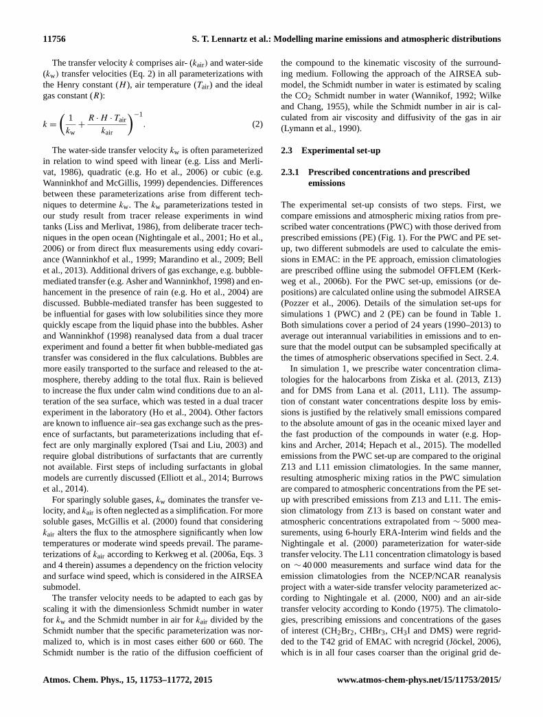
The experimental set-up consists of two steps. First, we
compare emissions and atmospheric mixing ratios from pre-
scribed water concentrations (PWC) with those derived from
prescribed emissions (PE) (Fig. 1). For the PWC and PE set-
up, two different submodels are used to calculate the emis-
sions in EMAC: in the PE approach, emission climatologies
are prescribed offline using the submodel OFFLEM (Kerk-
weg et al., 2006b). For the PWC set-up, emissions (or de-
positions) are calculated online using the submodel AIRSEA
(Pozzer et al., 2006). Details of the simulation set-ups for
simulations 1 (PWC) and 2 (PE) can be found in Table 1.
Both simulations cover a period of 24 years (1990–2013) to
average out interannual variabilities in emissions and to en-
sure that the model output can be subsampled specifically at
the times of atmospheric observations specified in Sect. 2.4.
In simulation 1, we prescribe water concentration clima-
tologies for the halocarbons from Ziska et al. (2013, Z13)
and for DMS from Lana et al. (2011, L11). The assump-
tion of constant water concentrations despite loss by emis-
sions is justified by the relatively small emissions compared
to the absolute amount of gas in the oceanic mixed layer and
the fast production of the compounds in water (e.g. Hop-
kins and Archer, 2014; Hepach et al., 2015). The modelled
emissions from the PWC set-up are compared to the original
Z13 and L11 emission climatologies. In the same manner,
resulting atmospheric mixing ratios in the PWC simulation
are compared to atmospheric concentrations from the PE set-
up with prescribed emissions from Z13 and L11. The emis-
sion climatology from Z13 is based on constant water and
atmospheric concentrations extrapolated from ∼ 5000 mea-
surements, using 6-hourly ERA-Interim wind fields and the
Nightingale et al. (2000) parameterization for water-side
transfer velocity. The L11 concentration climatology is based
on ∼ 40 000 measurements and surface wind data for the
emission climatologies from the NCEP/NCAR reanalysis
project with a water-side transfer velocity parameterized ac-
cording to Nightingale et al. (2000, N00) and an air-side
transfer velocity according to Kondo (1975). The climatolo-
gies, prescribing emissions and concentrations of the gases
of interest (CH2Br2, CHBr3, CH3I and DMS) were regrid-
ded to the T42 grid of EMAC with ncregrid (Jöckel, 2006),
which is in all four cases coarser than the original grid de-
Atmos. Chem. Phys., 15, 11753–11772, 2015 www.atmos-chem-phys.net/15/11753/2015/
S. T. Lennartz et al.: Modelling marine emissions and atmospheric distributions 11757
Fixed water concentrations (Z13, L11)
EMAC atmosphere
Fixed water concentrations
(Z13, L11)
Fixed atmospheric
vmr (Z13, L11)
EMAC atmosphere
Online flux calculation with
AIRSEA
Offline flux calculation
(Z13, L11)
Prescribed emissions (PE): Prescribed water concentration (PWC):
Pres
crib
ed
conc
entr
atio
ns
Pres
crib
ed
emiss
ions
with
O
FFLE
M
Figure 1. Schematic overview of the set-up of prescribed emissions (PE, left panel) and online-calculated fluxes based on prescribed water
concentrations (PWC, right panel) implemented in EMAC. Climatologies of fixed water and atmospheric concentrations in Ziska et al. (2013;
Z13) and Lana et al. (2011; L11) were used to compute a global emission estimate, and the resulting interannual mean emission climatology
is prescribed in EMAC using the submodule OFFLEM (PE, left panel). Calculating emissions online based on prescribed concentration (Z13,
L11) considers the current state of the atmosphere during the calculation of emissions in the submodule AIRSEA (PWC, right panel).
Table 1. Set-up of model simulations evaluated in this study. PWC: prescribed water concentration, PE: prescribed emissions, AIRSEA:
submodel for online calculation of emissions, OFFLEM: submodel for prescribing emissions.
Abbreviation kw- Emission calculation, Rain White cap Period
parameterization submodule effect coverage effect
1 PWC Nightingale et al. (2000) PWC, AIRSEA No No 1990–2013
2 PE Prescribed emissions, no online
calculation, kw in original pub-
lications N00
PE, OFFLEM No No 1990–2013
3 LM86 Liss and Merlivat (1986) PWC, AIRSEA No No 2010–2011
4 W99 Wanninkhof et al. (1999) PWC, AIRSEA No No 2010–2011
5 N00 Nightingale et al. (2000) PWC, AIRSEA No No 2010–2011
6 H06 Ho et al. (2006) PWC, AIRSEA No No 2010–2011
7 H06r Ho et al. (2006) PWC, AIRSEA Yes No 2010–2011
8 A98 Asher and Wanninkhof (1998) PWC, AIRSEA No Yes 2010–2011
9 B13m Bell et al. (2013) modified, only
DMS
PWC, AIRSEA No No 2004–2013
10 M09 Marandino et al. (2009) PWC, AIRSEA No No 2004–2013
scribed in Z13 and L11 (1◦× 1◦ in both). It has to be noted
that this leads to a smoothing of small, local hotspots, but we
assume this to be negligible since we compare emissions on
a global scale.
Besides the concentrations taken from the climatologies
Z13/L11, the air–sea calculation requires information on sea
surface temperature, salinity and wind. The mean sea sur-
face temperature in the model for simulation 1 (1990–2013)
was 15.95 ◦C, 15.82 ◦C in Z13 and 16.22 ◦C in L11. The
mean wind speed in the EMAC simulations (PWC, PE) was
7.51 m s−1, which is slightly larger than the wind speed used
to calculate the emission climatologies in Z13 (EMAC is
4.7 % larger) and L11 (EMAC is 2.7 % larger). Sea surface
salinity is prescribed with a constant value of 0.4 mol L−1 in
our model simulations as opposed to spatially varying salin-
ity in Z13 and L11. A 2-year simulation comparing the ef-
fects of a constant salinity versus the Z13 climatology re-
vealed a low effect on global emissions (< 3 %), which is in
accordance with findings of Ziska et al. (2013). Compared to
the calculation of the Schmidt number in the publications by
www.atmos-chem-phys.net/15/11753/2015/ Atmos. Chem. Phys., 15, 11753–11772, 2015
11758 S. T. Lennartz et al.: Modelling marine emissions and atmospheric distributions
Z13 and L11, the submodel AIRSEA uses a different empiri-
cal, temperature-dependent equation to calculate the Schmidt
number. In AIRSEA, the Schmidt number of CO2 at the re-
spective temperature is calculated and then adapted with the
molar volume to the Schmidt number of the gas of interest
(Wilke and Chang, 1955; Hayduk and Laudie, 1974). In Z13,
the Schmidt number is calculated by averaging the diffu-
sion coefficient according to Hayduk and Laudie (1974) and
Wilke and Chang (1955) and then dividing by the dynamic
viscosity of seawater at varying temperatures and a constant
salinity of 35. In L11, the Schmidt number is calculated ac-
cording to Saltzman et al. (1993). The resulting differences
are negligible at sea surface temperatures higher than 10 ◦C
and grow largest at 0 ◦C, where they are still less than 15 %.
Since the Schmidt number is then normalized to the Schmidt
number of CO2, the resulting difference becomes small and
does not lead to significant differences in the global emission
estimates of all four compounds. Differences in other influ-
ential input parameters for emission calculation between our
PWC set-up and Z13 and L11 are thus small, ensuring that
differences in emissions between PWC and Z13 and L11 can
be attributed to the consideration of the actual state of the
atmosphere in the PWC set-up.
2.3.2 Transfer velocity parameterizations
In the second part of the study, we test the sensitivity of the
global emissions towards eight different transfer velocity pa-
rameterizations. These tests cover a 2-year time span (2010–
2011) with 1 year (2009) as spin-up. The simulations 3–6
(Table 1) test the impact of different water-side transfer ve-
locity parameterizations related to wind speed. The parame-
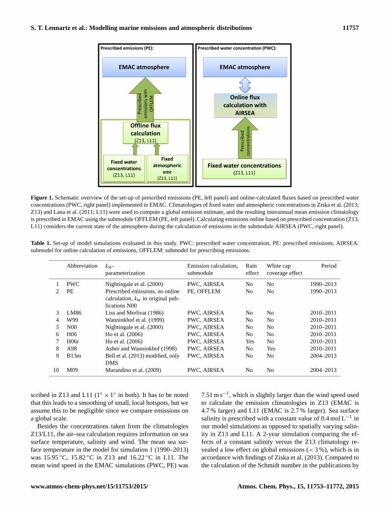
terizations tested in this study are illustrated in Fig. 2. With
increasing wind speed, the differences between the transfer
velocity parameterizations grow larger; hence, testing these
parameterizations yields a range of global emission estimates
that reflects this uncertainty. Parameterizations and the gen-
eral description of air–sea gas exchange calculation are de-
scribed in Sect. 2.2.
Table 1 provides an overview of all performed simulations.
Simulation 3 uses the 3-step linear parameterization of Liss
and Merlivat (1986, LM86), simulation 4 the cubic relation-
ship by Wanninkhof and McGillis (1999, W99), simulation
5 the quadratic parameterization by Nightingale et al. (2000,
N00), and simulation 6 the quadratic transfer velocity param-
eterization by Ho et al. (2006, H06). The effect of rain (simu-
lation 7 in Table 1) was tested adding the Ho et al. (1997) rain
effect parameterization to the H06 transfer velocity parame-
terization (see Pozzer et al., 2006, Eqs. 10 and 11). White cap
coverage according to Asher and Wanninkhof (1998, A98)
considers bubble-mediated gas exchange and is used in simu-
lation 8. The different parameterizations (LM86, W99, N00,
H06) were available from the AIRSEA version of Pozzer
et al. (2006). The N00 parameterization was normalized to
wind speed [m s-1]
0 5 10 15 20
k 660 [c
m h
r-1]
0
50
100
150
200
250LM86W99N00H06B13m
Figure 2. Parameterizations for water-side transfer velocity of air–
sea gas exchange kw for a Schmidt number of 660 that are tested
in this study: the linear parameterization LM96 (Liss and Merlivat,
1986), the cubic parameterization W99 (Wanninkhof and McGillis,
1999), the quadratic parameterization N00 (Nightingale et al., 2000)
and H06 (Ho et al., 2006), the parameterization modified according
to Bell et al. (2013, B13m) with a levelling off at wind speeds higher
than 11 m s−1, and the linear parameterization M09 (Marandino et
al., 2009).
the Schmidt number of 600 as in the original publication by
Nightingale et al. (2000), while 660 was used in Z13.
Two additional simulations including only DMS were per-
formed to test the effect of two recently published parame-
terizations of kw. These two parameterizations have been de-
rived from in situ DMS eddy covariance measurements and
deviate from previously published parameterizations. Bell et
al. (2003) observed that the transfer velocity does not in-
crease at wind speeds higher than 11 m s−1. Marandino et
al. (2009) found a linear dependency between wind speed
and the transfer velocity kw for DMS. Both simulations cover
the period of 2004–2013, since observations from this period
were available for comparison. These two parameterizations
for kw were added to the submodule code of AIRSEA (for
equations see Table 4). The modification of the code included
a parameterization based on results of the study from Bell
et al. (2013, B13m) with a conservative approach, in which
the N00 parameterization was used at wind speeds below
11 m s−1 and kept constant at higher wind speeds to account
for the missing increase of kw with increasing wind speed. Fi-
nally, the parameterization by Marandino et al. (2009, M09)
was used in simulation 10 for the same period as B13m. Both
newly implemented parameterizations are part of the most
recent release MESSy 2.52.
2.4 Observational data
Simulated atmospheric mixing ratios of the trace gases from
PWC and PE are compared to observations from ship cam-
Atmos. Chem. Phys., 15, 11753–11772, 2015 www.atmos-chem-phys.net/15/11753/2015/
S. T. Lennartz et al.: Modelling marine emissions and atmospheric distributions 11759
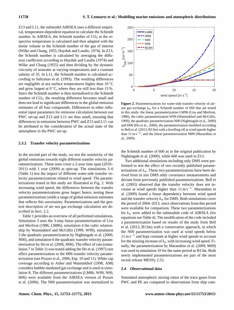
Figure 3. Locations of atmospheric data for comparison with model output used in this study. Panel (a) shows locations of atmospheric
measurements from 23 aircraft campaigns considered for comparison with halocarbon simulations. Panel (b) shows location of measurements
in the atmospheric boundary layer from ships (PHASE-1, Knorr-06, Knorr-07, M98) and from aircraft campaign (HIPPO 1–5) measurements
considered for comparison with DMS simulations.
paigns, aircraft campaigns and ground-based time series sta-
tions.
A total of 23 aircraft campaigns providing halocarbon data
are considered in order to create annual zonal mean clima-
tologies of these trace gases. The combined data set ranges
from 90◦ N to 75◦ S, transecting from the surface to the
upper troposphere/lower stratosphere over land and ocean
from 1992 to 2012 (see Table S1 for details on the aircraft
campaigns). Many of the more recent data sets are inter-
calibrated (see e.g. Brinckmann et al., 2012; Hall et al., 2014;
Sala et al., 2014; Wisher et al., 2014). The latitudinal and lon-
gitudinal distributions and names of the aircraft campaigns
are illustrated in Fig. 3a. The measurements were averaged
in zonal 10◦ wide latitude bins with a vertical extent ranging
from 10 to 50 hPa (10 hPa in boundary layer and TTL re-
gions). Most of the measurements are located around 30◦ N
of latitude with more than 150 points per bin. The tropical
region (20◦ N–20◦ S) has an average of 50 points per bin.
Figure S1 in the Supplement illustrates the numbers of the
measurements per bin. For the comparison of measured and
modelled data, the EMAC output of simulations 1 and 2 is
first sampled at the same location as the aircraft measure-
ments (longitude, latitude, altitude and time) by linear inter-
polation. Then, the same process of averaging per bin as for
the measurements is applied to the model output.
Nine coastal ground stations from NOAA/ESRL, where
halocarbons have been measured by the NOAA global flask
sampling network starting from 1990–2004 were chosen for
comparison due to their location close to the coast (Table 2).
These data are currently available at the HalOcAt (Halocar-
bons in the Ocean and Atmosphere) database (https://halocat.
geomar.de/). Two time series stations situated distant to the
coast (Park Falls, Wisconsin, Niwot Ridge Forest, Colorado,
both USA) were chosen to assess to contribution of marine
www.atmos-chem-phys.net/15/11753/2015/ Atmos. Chem. Phys., 15, 11753–11772, 2015
11760 S. T. Lennartz et al.: Modelling marine emissions and atmospheric distributions
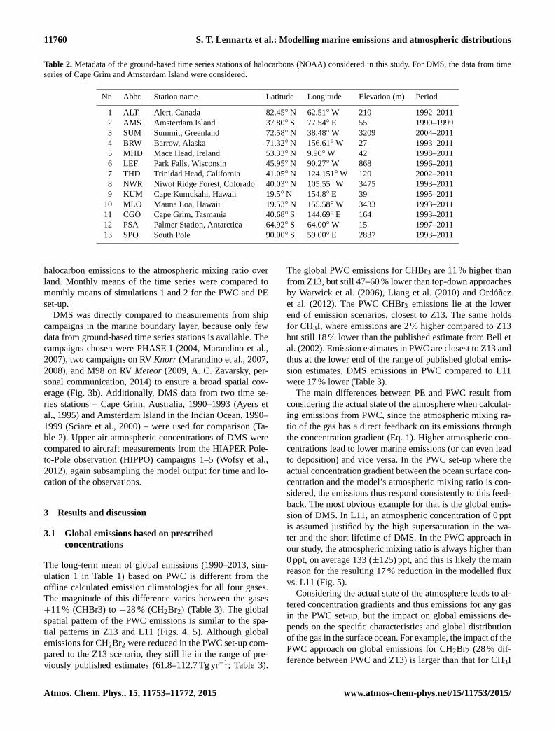
Table 2. Metadata of the ground-based time series stations of halocarbons (NOAA) considered in this study. For DMS, the data from time
series of Cape Grim and Amsterdam Island were considered.
Nr. Abbr. Station name Latitude Longitude Elevation (m) Period
1 ALT Alert, Canada 82.45◦ N 62.51◦W 210 1992–2011
2 AMS Amsterdam Island 37.80◦ S 77.54◦ E 55 1990–1999
3 SUM Summit, Greenland 72.58◦ N 38.48◦W 3209 2004–2011
4 BRW Barrow, Alaska 71.32◦ N 156.61◦W 27 1993–2011
5 MHD Mace Head, Ireland 53.33◦ N 9.90◦W 42 1998–2011
6 LEF Park Falls, Wisconsin 45.95◦ N 90.27◦W 868 1996–2011
7 THD Trinidad Head, California 41.05◦ N 124.151◦W 120 2002–2011
8 NWR Niwot Ridge Forest, Colorado 40.03◦ N 105.55◦W 3475 1993–2011
9 KUM Cape Kumukahi, Hawaii 19.5◦ N 154.8◦ E 39 1995–2011
10 MLO Mauna Loa, Hawaii 19.53◦ N 155.58◦W 3433 1993–2011
11 CGO Cape Grim, Tasmania 40.68◦ S 144.69◦ E 164 1993–2011
12 PSA Palmer Station, Antarctica 64.92◦ S 64.00◦W 15 1997–2011
13 SPO South Pole 90.00◦ S 59.00◦ E 2837 1993–2011
halocarbon emissions to the atmospheric mixing ratio over
land. Monthly means of the time series were compared to
monthly means of simulations 1 and 2 for the PWC and PE
set-up.
DMS was directly compared to measurements from ship
campaigns in the marine boundary layer, because only few
data from ground-based time series stations is available. The
campaigns chosen were PHASE-I (2004, Marandino et al.,
2007), two campaigns on RV Knorr (Marandino et al., 2007,
2008), and M98 on RV Meteor (2009, A. C. Zavarsky, per-
sonal communication, 2014) to ensure a broad spatial cov-
erage (Fig. 3b). Additionally, DMS data from two time se-
ries stations – Cape Grim, Australia, 1990–1993 (Ayers et
al., 1995) and Amsterdam Island in the Indian Ocean, 1990–
1999 (Sciare et al., 2000) – were used for comparison (Ta-
ble 2). Upper air atmospheric concentrations of DMS were
compared to aircraft measurements from the HIAPER Pole-
to-Pole observation (HIPPO) campaigns 1–5 (Wofsy et al.,
2012), again subsampling the model output for time and lo-
cation of the observations.
3 Results and discussion
3.1 Global emissions based on prescribed
concentrations
The long-term mean of global emissions (1990–2013, sim-
ulation 1 in Table 1) based on PWC is different from the
offline calculated emission climatologies for all four gases.
The magnitude of this difference varies between the gases
+11 % (CHBr3) to −28 % (CH2Br2) (Table 3). The global
spatial pattern of the PWC emissions is similar to the spa-
tial patterns in Z13 and L11 (Figs. 4, 5). Although global
emissions for CH2Br2 were reduced in the PWC set-up com-
pared to the Z13 scenario, they still lie in the range of pre-
viously published estimates (61.8–112.7 Tg yr−1; Table 3).
The global PWC emissions for CHBr3 are 11 % higher than
from Z13, but still 47–60 % lower than top-down approaches
by Warwick et al. (2006), Liang et al. (2010) and Ordóñez
et al. (2012). The PWC CHBr3 emissions lie at the lower
end of emission scenarios, closest to Z13. The same holds
for CH3I, where emissions are 2 % higher compared to Z13
but still 18 % lower than the published estimate from Bell et
al. (2002). Emission estimates in PWC are closest to Z13 and
thus at the lower end of the range of published global emis-
sion estimates. DMS emissions in PWC compared to L11
were 17 % lower (Table 3).
The main differences between PE and PWC result from
considering the actual state of the atmosphere when calculat-
ing emissions from PWC, since the atmospheric mixing ra-
tio of the gas has a direct feedback on its emissions through
the concentration gradient (Eq. 1). Higher atmospheric con-
centrations lead to lower marine emissions (or can even lead
to deposition) and vice versa. In the PWC set-up where the
actual concentration gradient between the ocean surface con-
centration and the model’s atmospheric mixing ratio is con-
sidered, the emissions thus respond consistently to this feed-
back. The most obvious example for that is the global emis-
sion of DMS. In L11, an atmospheric concentration of 0 ppt
is assumed justified by the high supersaturation in the wa-
ter and the short lifetime of DMS. In the PWC approach in
our study, the atmospheric mixing ratio is always higher than
0 ppt, on average 133 (±125) ppt, and this is likely the main
reason for the resulting 17 % reduction in the modelled flux
vs. L11 (Fig. 5).
Considering the actual state of the atmosphere leads to al-
tered concentration gradients and thus emissions for any gas
in the PWC set-up, but the impact on global emissions de-
pends on the specific characteristics and global distribution
of the gas in the surface ocean. For example, the impact of the
PWC approach on global emissions for CH2Br2 (28 % dif-
ference between PWC and Z13) is larger than that for CH3I
Atmos. Chem. Phys., 15, 11753–11772, 2015 www.atmos-chem-phys.net/15/11753/2015/

S. T. Lennartz et al.: Modelling marine emissions and atmospheric distributions 11761
A C
B D
Figure 4. Emissions from PWC (N00 parameterization for kw) for the trace gases dibromomethane (CH2Br2, panel a), bromoform (CHBr3,
panel b), methyliodide (CH3I, panel c) and dimethyl sulfide (DMS, panel d), their annual mean of the period 1990–2013 (simulation 1,
Table 1).
(2 % difference) (Table 3). This difference can be explained
by the saturation of the two gases: CH3I is mainly oversat-
urated in the surface ocean with a mean saturation ratio (ac-
tual concentration divided by equilibrium concentration) of
18.2 in Z13. CH2Br2 with a mean saturation ratio of 2 is
concentrated closer to equilibrium. The distance from equi-
librium is thus larger for CH3I than for CH2Br2. Changes in
atmospheric mixing ratio therefore affect the concentration
gradient for CH2Br2 more than for CH3I. For CHBr3 with
a similar global ocean surface saturation ratio as CH2Br2, a
drastic change in emissions between PWC and Z13 can be
seen in the Southern Hemisphere (50–90◦ S; Table 3), where
the emissions increase 2 orders of magnitude in the PWC
compared to Z13. The Z13 emission climatology displays a
latitudinal band of elevated atmospheric mixing ratios around
60◦ S, which result in this region being a sink for atmospheric
CHBr3. In our PWC set-up, atmospheric mixing ratios in this
region are not as elevated and hence PWC leads to larger
emissions. In general, gases that are concentrated close to
equilibrium in the surface ocean respond more strongly to
changes in atmospheric concentrations and thus to the PWC
set-up than more supersaturated gases.
Comparing integrated regional fluxes, the halocarbons dis-
play the largest differences in the polar regions (Table 3).
Besides dynamic atmospheric concentrations that may alter
emissions in the PE set-up, two other reasons for differences
in this specific set-up apply for the halocarbons. First, no sea
ice is considered in Z13 whereas EMAC uses prescribed sea
ice in our PWC set-up. L11 considers sea-ice. When sea ice is
present in the model EMAC/AIRSEA, the flux is reduced by
the fraction of surface that is covered by it. This may lead to
the lower flux estimations in our PWC set-up and may partly
explain e.g. the reduced emissions in the Arctic for CHBr3.
Furthermore, our PWC approach takes into account air-side
transfer velocity (Eq. 2) instead of only the water-side trans-
fer velocity as Z13, which can control the flux of more sol-
uble gases at low temperatures and thus decrease emissions
(McGillis et al., 2000). At high latitudes (60–90◦ N and S),
where low temperatures and high winds prevail, the trans-
fer velocity can be reduced by up to 68 % (CH2Br2), 32 %
(CHBr3) and 61 % (CH3I) using kair in the PWC set-up. L11
takes the kair and sea ice into account, so this difference does
not apply.
3.2 Atmospheric mixing ratios based on PWC and PE
The atmospheric mixing ratios in EMAC sustained by emis-
sions either from PWC or PE are compared to available atmo-
spheric observations from aircraft campaigns (halocarbons,
DMS), ground-based time series stations from NOAA/ESRL
(halocarbons) and ship campaigns (DMS). The model output
of simulations 1 and 2 (Tables 1, 4) was subsampled at the
times and locations of the observations. A scatterplot for di-
rect comparison between model output and observations is
provided in the Supplement in Fig. S2.
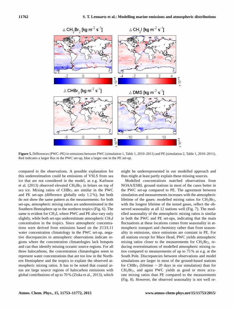
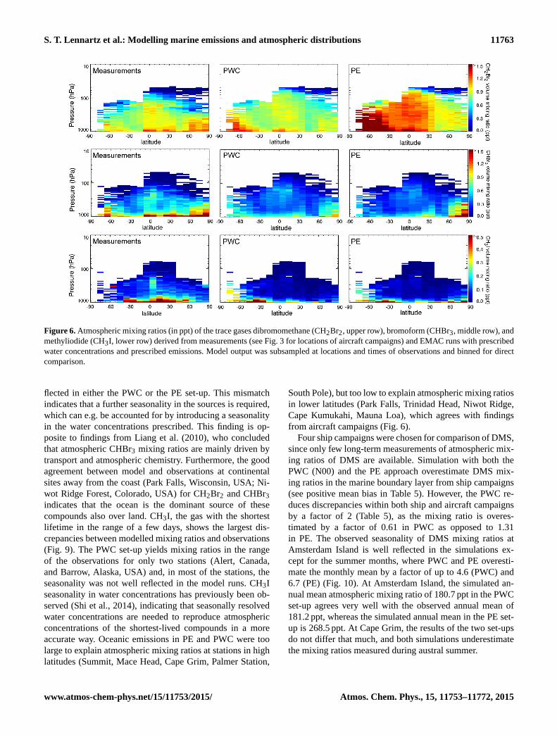
The largest difference between PWC and PE in the at-
mospheric mixing ratio is again found for CH2Br2 in the
Southern Hemisphere (Fig. 6), where the PWC set-up yields
lower emissions and therefore also lower atmospheric mixing
ratios. For CH2Br2, atmospheric mixing ratios globally de-
crease on average by 28 % compared to the PE set-up, which
is the same percentage as the reduction in the global emis-
sions. Concentrations derived from these reduced fluxes gen-
erally agree better with the measurements, even though Arc-
tic emissions still seem to be underestimated in the model
www.atmos-chem-phys.net/15/11753/2015/ Atmos. Chem. Phys., 15, 11753–11772, 2015
11762 S. T. Lennartz et al.: Modelling marine emissions and atmospheric distributions
Figure 5. Differences (PWC–PE) in emissions between PWC (simulation 1, Table 1, 2010–2011) and PE (simulation 2, Table 1, 2010–2011).
Red indicates a larger flux in the PWC set-up, blue a larger one in the PE set-up.
compared to the observations. A possible explanation for
this underestimation could be emissions of VSLS from sea
ice that are not considered in the model, as e.g. Karlsson
et al. (2013) observed elevated CH2Br2 in brines on top of
sea ice. Mixing ratios of CHBr3 are similar in the PWC
and PE set-ups (difference globally only 1.2 %), but both
do not show the same pattern as the measurements: for both
set-ups, atmospheric mixing ratios are underestimated in the
Southern Hemisphere up to the northern tropics (Fig. 6). The
same is evident for CH3I, where PWC and PE also vary only
slightly, while both set-ups underestimate atmospheric CH3I
concentration in the tropics. Since atmospheric concentra-
tions were derived from emissions based on the Z13/L11
water concentration climatology in the PWC set-up, nega-
tive discrepancies to atmospheric observations indicate re-
gions where the concentration climatologies lack hotspots
and can thus identify missing oceanic source regions. For all
three halocarbons, the concentration climatologies seem to
represent water concentrations that are too low in the North-
ern Hemisphere and the tropics to explain the observed at-
mospheric mixing ratios. It has to be noted that coastal ar-
eas are large source regions of halocarbon emissions with
global contributions of up to 70 % (Ziska et al., 2013), which
might be underrepresented in our modelled approach and
thus might at least partly explain these missing sources.
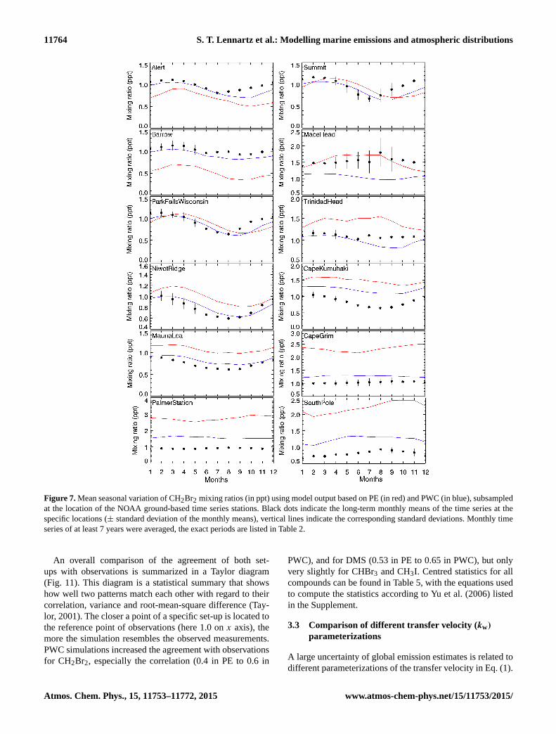
Modelled concentrations matched observations from
NOAA/ESRL ground stations in most of the cases better in
the PWC set-up compared to PE. The agreement between
simulation and measurements increases with the atmospheric
lifetime of the gases: modelled mixing ratios for CH2Br2,
with the longest lifetime of the tested gases, reflect the ob-
served seasonality at all 12 stations well (Fig. 7). The mod-
elled seasonality of the atmospheric mixing ratios is similar
in both the PWC and PE set-ups, indicating that the main
fluctuations at these locations comes from seasonality in at-
mospheric transport and chemistry rather than from season-
ality in emissions, since emissions are constant in PE. For
all stations except for Mace Head, PWC yields atmospheric
mixing ratios closer to the measurements for CH2Br2, re-
ducing overestimations of modelled atmospheric mixing ra-
tios compared to measurements of up to 75 % as e.g. at the
South Pole. Discrepancies between observations and model
simulations are larger in most of the ground-based stations
for CHBr3 (lifetime ∼ 20 days in our simulation) than for
CH2Br2, and again PWC yields as good or more accu-
rate mixing ratios than PE compared to the measurements
(Fig. 8). However, the observed seasonality is not well re-
Atmos. Chem. Phys., 15, 11753–11772, 2015 www.atmos-chem-phys.net/15/11753/2015/
S. T. Lennartz et al.: Modelling marine emissions and atmospheric distributions 11763
Figure 6. Atmospheric mixing ratios (in ppt) of the trace gases dibromomethane (CH2Br2, upper row), bromoform (CHBr3, middle row), and
methyliodide (CH3I, lower row) derived from measurements (see Fig. 3 for locations of aircraft campaigns) and EMAC runs with prescribed
water concentrations and prescribed emissions. Model output was subsampled at locations and times of observations and binned for direct
comparison.
flected in either the PWC or the PE set-up. This mismatch
indicates that a further seasonality in the sources is required,
which can e.g. be accounted for by introducing a seasonality
in the water concentrations prescribed. This finding is op-
posite to findings from Liang et al. (2010), who concluded
that atmospheric CHBr3 mixing ratios are mainly driven by
transport and atmospheric chemistry. Furthermore, the good
agreement between model and observations at continental
sites away from the coast (Park Falls, Wisconsin, USA; Ni-
wot Ridge Forest, Colorado, USA) for CH2Br2 and CHBr3
indicates that the ocean is the dominant source of these
compounds also over land. CH3I, the gas with the shortest
lifetime in the range of a few days, shows the largest dis-
crepancies between modelled mixing ratios and observations
(Fig. 9). The PWC set-up yields mixing ratios in the range
of the observations for only two stations (Alert, Canada,
and Barrow, Alaska, USA) and, in most of the stations, the
seasonality was not well reflected in the model runs. CH3I
seasonality in water concentrations has previously been ob-
served (Shi et al., 2014), indicating that seasonally resolved
water concentrations are needed to reproduce atmospheric
concentrations of the shortest-lived compounds in a more
accurate way. Oceanic emissions in PE and PWC were too
large to explain atmospheric mixing ratios at stations in high
latitudes (Summit, Mace Head, Cape Grim, Palmer Station,
South Pole), but too low to explain atmospheric mixing ratios
in lower latitudes (Park Falls, Trinidad Head, Niwot Ridge,
Cape Kumukahi, Mauna Loa), which agrees with findings
from aircraft campaigns (Fig. 6).
Four ship campaigns were chosen for comparison of DMS,
since only few long-term measurements of atmospheric mix-
ing ratios of DMS are available. Simulation with both the
PWC (N00) and the PE approach overestimate DMS mix-
ing ratios in the marine boundary layer from ship campaigns
(see positive mean bias in Table 5). However, the PWC re-
duces discrepancies within both ship and aircraft campaigns
by a factor of 2 (Table 5), as the mixing ratio is overes-
timated by a factor of 0.61 in PWC as opposed to 1.31
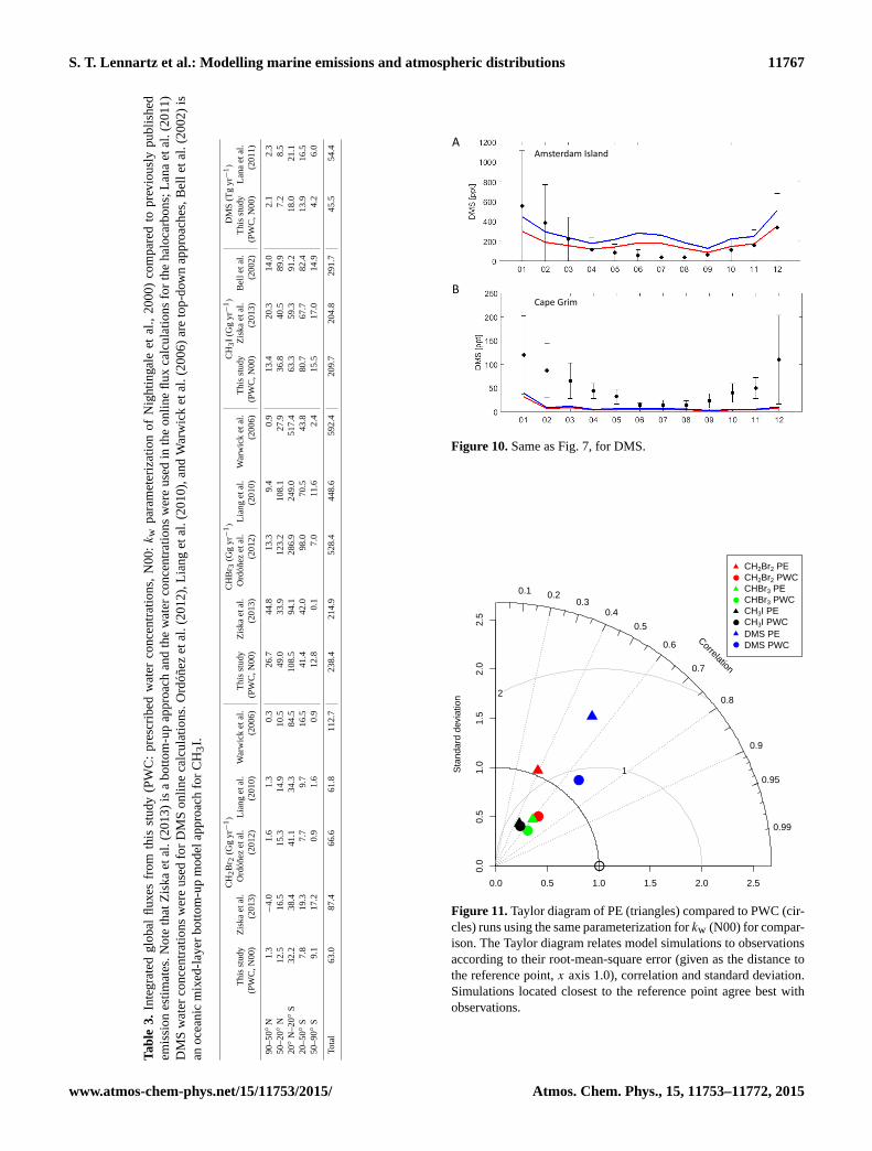
in PE. The observed seasonality of DMS mixing ratios at
Amsterdam Island is well reflected in the simulations ex-
cept for the summer months, where PWC and PE overesti-
mate the monthly mean by a factor of up to 4.6 (PWC) and
6.7 (PE) (Fig. 10). At Amsterdam Island, the simulated an-
nual mean atmospheric mixing ratio of 180.7 ppt in the PWC
set-up agrees very well with the observed annual mean of
181.2 ppt, whereas the simulated annual mean in the PE set-
up is 268.5 ppt. At Cape Grim, the results of the two set-ups
do not differ that much, and both simulations underestimate
the mixing ratios measured during austral summer.
www.atmos-chem-phys.net/15/11753/2015/ Atmos. Chem. Phys., 15, 11753–11772, 2015
11764 S. T. Lennartz et al.: Modelling marine emissions and atmospheric distributions
Figure 7. Mean seasonal variation of CH2Br2 mixing ratios (in ppt) using model output based on PE (in red) and PWC (in blue), subsampled
at the location of the NOAA ground-based time series stations. Black dots indicate the long-term monthly means of the time series at the
specific locations (± standard deviation of the monthly means), vertical lines indicate the corresponding standard deviations. Monthly time
series of at least 7 years were averaged, the exact periods are listed in Table 2.
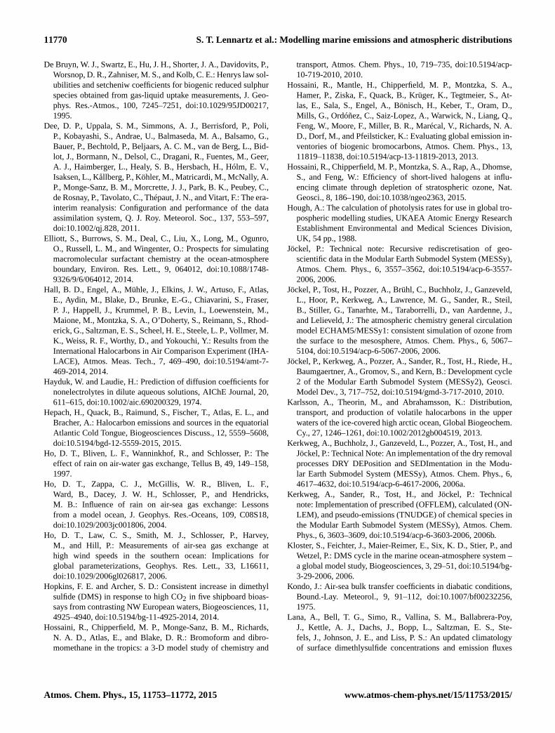
An overall comparison of the agreement of both set-
ups with observations is summarized in a Taylor diagram
(Fig. 11). This diagram is a statistical summary that shows
how well two patterns match each other with regard to their
correlation, variance and root-mean-square difference (Tay-
lor, 2001). The closer a point of a specific set-up is located to
the reference point of observations (here 1.0 on x axis), the
more the simulation resembles the observed measurements.
PWC simulations increased the agreement with observations
for CH2Br2, especially the correlation (0.4 in PE to 0.6 in
PWC), and for DMS (0.53 in PE to 0.65 in PWC), but only
very slightly for CHBr3 and CH3I. Centred statistics for all
compounds can be found in Table 5, with the equations used
to compute the statistics according to Yu et al. (2006) listed
in the Supplement.
3.3 Comparison of different transfer velocity (kw)
parameterizations
A large uncertainty of global emission estimates is related to
different parameterizations of the transfer velocity in Eq. (1).
Atmos. Chem. Phys., 15, 11753–11772, 2015 www.atmos-chem-phys.net/15/11753/2015/

S. T. Lennartz et al.: Modelling marine emissions and atmospheric distributions 11765
Figure 8. Same as Fig. 7, for CHBr3.
Calculating emissions online enables a simple way of testing
different transfer velocity parameterizations, which was real-
ized here with eight 2-year simulations described in Table 1
(simulations 3–10).
The largest sensitivity for the emissions of all gases is
introduced by different parameterizations of the water-side
transfer velocity kw tested in simulations 3–6 (Table 4). The
4 parameterizations that were tested (simulation 3–6, Ta-
ble 1) comprised linear (LM86, simulation 3), cubic (W99,
simulation 4) and quadratic (N00, simulation 5, H06, sim-
ulation 6) relations to wind speed. The resulting global
emission estimates in these parameterizations range 53.7–
65.1 Gg yr−1 for CH2Br2, 189.0–249.7 Gg yr−1 for CHBr3,
151.9–225.7 Gg yr−1 for CH3I and 33.4–48.7 Tg yr−1 for
DMS (Table 4). As expected, the linear kw parameterization
(LM86) yields the lowest global emission estimates, since
it produces the lowest kw values (Fig. 2). The N00 parame-
terization produces the highest global fluxes for CHBr3 and
CH2Br2 but not for DMS and CH3I, where the highest fluxes
were obtained by H06 (DMS) and W99 (CH3I) (Table 4).
The fact that different parameterizations lead to higher global
estimates for different gases is explained by the varying spa-
tial distribution of concentration hot spots and regional vari-
ations of wind.
The kw parameterization in simulation 7 increases the flux
under calm conditions due to precipitation. This increase
www.atmos-chem-phys.net/15/11753/2015/ Atmos. Chem. Phys., 15, 11753–11772, 2015

11766 S. T. Lennartz et al.: Modelling marine emissions and atmospheric distributions
Figure 9. Same as Fig. 7, for CH3I.
ranged from 4 % (CH2Br2) to 6 % (DMS) (Table 4) when
compared to the reference flux using H06 alone (simula-
tion 6, Table 4). Additional flux due to precipitation is in-
versely correlated to the Schmidt number, so that under iden-
tical conditions, increasing flux would be added in the order
CHBr3 > CH2Br2 > DMS > CH3I. The global flux estima-
tions compared to the reference run do not increase in this or-
der (Table 4), rather DMS > CHBr3∼CH3I > CH2Br2. This
non-uniform response among the gases is explained by the
globally and regionally varying distance from equilibrium
for the four gases, which together with regional precipita-
tion patterns leads to variations in the emissions increased
by rain. The parameterization based on white-cap coverage
(A98) also has small but ambivalent effects on the global flux
for the different compounds (simulation 8, Table 4). Com-
pared to the mean of all nonlinear parameterizations for each
gas, global emissions were higher when the white cap cover-
age parameterization was used for CHBr3 (4 %) and CH2Br2
(2 %) but lower for CH3I (−8 %) and DMS (−6 %) (Table 4).
The parameterizations tested only for DMS are both de-
rived from eddy covariance measurements at sea. Both pa-
rameterizations changed the global emissions by −4.4 %
(B13m) and −1.2 % (M09) compared to the average flux
of simulations 3–6 (Table 4). Although the modelled atmo-
spheric mixing ratios at the time and location of observations
is for both of the parameterizations higher than the observa-
Atmos. Chem. Phys., 15, 11753–11772, 2015 www.atmos-chem-phys.net/15/11753/2015/
S. T. Lennartz et al.: Modelling marine emissions and atmospheric distributions 11767
Ta
ble
3.
Inte
gra
ted
glo
bal
flu
xes
fro
mth
isst
ud
y(P
WC
:p
resc
rib
edw
ater
con
cen
trat
ion
s,N
00
:k
wp
aram
eter
izat
ion
of
Nig
hti
ngal
eet
al.,
20
00
)co
mp
ared
top
rev
iou
sly
pu
bli
shed
emis
sio
nes
tim
ates
.N
ote
that
Zis
ka
etal
.(2
01
3)
isa
bo
tto
m-u
pap
pro
ach
and
the
wat
erco
nce
ntr
atio
ns
wer
eu
sed
inth
eo
nli
ne
flu
xca
lcu
lati
on
sfo
rth
eh
alo
carb
on
s;L
ana
etal
.(2
01
1)
DM
Sw
ater
con
cen
trat
ion
sw
ere
use
dfo
rD
MS
on
lin
eca
lcu
lati
on
s.O
rdó
ñez
etal
.(2
01
2),
Lia
ng
etal
.(2
01
0),
and
War
wic
ket
al.
(20
06
)ar
eto
p-d
ow
nap
pro
ach
es,
Bel
let
al.
(20
02
)is
ano
cean
icm
ixed
-lay
erb
ott
om
-up
mo
del
app
roac
hfo
rC
H3I.
CH
2B
r 2(G
gy
r−1)
CH
Br 3
(Gg
yr−
1)
CH
3I
(Gg
yr−
1)
DM
S(T
gy
r−1)
Th
isst
ud
yZ
isk
aet
al.
Ord
óñ
ezet
al.
Lia
ng
etal
.W
arw
ick
etal
.T
his
stu
dy
Zis
ka
etal
.O
rdó
ñez
etal
.L
ian
get
al.
War
wic
ket
al.
Th
isst
ud
yZ
isk
aet
al.
Bel
let
al.
Th
isst
ud
yL
ana
etal
.
(PW
C,
N0
0)
(20
13
)(2
01
2)
(20
10
)(2
00
6)
(PW
C,
N0
0)
(20
13
)(2
01
2)
(20
10
)(2
00
6)
(PW
C,
N0
0)
(20
13
)(2
00
2)
(PW
C,
N0
0)
(20
11
)
90
–5
0◦
N1
.3−
4.0
1.6
1.3
0.3
26
.74
4.8
13
.39
.40
.91
3.4
20
.31
4.0
2.1
2.3
50
–2
0◦
N1
2.5
16
.51
5.3
14
.91
0.5
49
.03
3.9
12
3.2
10
8.1
27
.93
6.8
40
.58
9.9
7.2
8.5
20◦
N–
20◦
S3
2.2
38
.44
1.1
34
.38
4.5
10
8.5
94
.12
86
.92
49
.05
17
.46
3.3
59
.39
1.2
18
.02
1.1
20
–5
0◦
S7
.81
9.3
7.7
9.7
16
.54
1.4
42
.09
8.0
70
.54
3.8
80
.76
7.7
82
.41
3.9
16
.5
50
–9
0◦
S9
.11
7.2
0.9
1.6
0.9
12
.80
.17
.01
1.6
2.4
15
.51
7.0
14
.94
.26
.0
To
tal
63
.08
7.4
66
.66
1.8
11
2.7
23
8.4
21
4.9
52
8.4
44
8.6
59
2.4
20
9.7
20
4.8
29
1.7
45
.55
4.4
A
B
Amsterdam Island
Cape Grim
Figure 10. Same as Fig. 7, for DMS.S
tand
ard
devi
atio
n
0.0 0.5 1.0 1.5 2.0 2.5
0.0
0.5
1.0
1.5
2.0
2.5
1
2
●
0.1 0.20.3
0.4
0.5
0.6
0.7
0.8
0.9
0.95
0.99
Correlation
●
●
●●
●
●
●
●
CH2Br2 PECH2Br2 PWCCHBr3 PECHBr3 PWCCH3I PECH3I PWCDMS PEDMS PWC
Figure 11. Taylor diagram of PE (triangles) compared to PWC (cir-
cles) runs using the same parameterization for kw (N00) for compar-
ison. The Taylor diagram relates model simulations to observations
according to their root-mean-square error (given as the distance to
the reference point, x axis 1.0), correlation and standard deviation.
Simulations located closest to the reference point agree best with
observations.
www.atmos-chem-phys.net/15/11753/2015/ Atmos. Chem. Phys., 15, 11753–11772, 2015

11768 S. T. Lennartz et al.: Modelling marine emissions and atmospheric distributions
Table 4. Integrated global emissions during 2010–2011 for sensitivity tests using different parameterizations for the transfer velocity kw
(simulations 3–6, same as in Table 1) and the effects of rain (simulation 7), bubble-mediated transfer parameterized using white cap coverage
(simulation 8) and parameterizations recently suggested for DMS (simulations 9 and 10). Equations for the parameterizations using wind
speed u are given for the Schmidt number (subscript after k) as in the original publications listed. u: wind speed at 10 m a.s.l. in metres per
second. k is given in centimetres per hour.
No. Parameterization CH2Br2 CHBr3 CH3I DMS
Gg yr−1 Gg yr−1 Gg yr−1 Tg yr−1
3 Liss and Merlivat (1986) for u≤ 3.6, k660 = 0.17u
for 3.6 < u< 13, k660 = 2.85u− 9.65
for u≥ 13, k660 = 5.9u
53.74 189.10 151.88 33.38
4 Wanninkhof et al. (1999) k660 = 0.0283u3 58.38 211.17 223.52 45.22
5 Nightingale et al. (2000) k600 = 0.22u2+ 0.333u 63.04 238.46 209.73 45.49
6 Ho et al. (2006) k660 = 0.266u2 62.71 236.10 213.47 45.91
7 Ho et al. (2006) + rain – 65.08 249.66 225.67 48.70
8 White cap coverage – 62.76 238.51 197.44 42.53
9 Bell et al. (2013), modified for u≤11, k600 = 0.22u2+ 0.333u
for u > 11, k600 = 30.283
– – – 40.63
10 Marandino et al. (2009) k720 = 1.92u− 1.0∗ – – – 42.45
Mean (simulations 3–6) 59.47 218.71 199.65 42.5
* Units converted, in original publication: k720 = 0.46u− 0.24 (m day−1).
Table 5. Error metrics for the comparison of model output from PWC (simulation 1) and PE (simulation 2) for all of the compounds
including all aircraft campaigns and ship observations, illustrated in Fig. S2 in the Supplement. Determination of error metrics according to
Yu et al. (2006).
CH2Br2 PE CH2Br2 PWC CHBr3 PE CHBr3 PWC CH3I PE CH3I PWC DMS PE DMS PWC
Mean bias (ppt) 0.24 −0.036 −0.23 −0.24 −0.14 −0.14 86.21 42.12
Mean absolute gross error (ppt) 0.30 0.15 0.31 0.31 0.15 0.16 102.9 67.39
RMSE (ppt) 0.381 0.21 0.53 0.53 0.26 0.26 236.2 135.8
Fractional bias (ppt) 0.26 0.0001 −0.23 −0.20 −0.89 −0.96 0.23 0.10
Fractional absolute error (ppt) 0.31 0.20 0.56 0.56 1.13 1.19 1.23 1.18
Normalized mean bias factor (–) 0.27 −0.04 −0.49 −0.53 −1.71 −1.96 1.31 0.64
tions, discrepancies between simulated and observed mixing
ratios were reduced compared to the N00 parameterization
by factors of 1.4 (B13m) and 1.2 (M09).
4 Summary and conclusions
Two different ways of considering marine emissions of trace
gases in global atmospheric chemistry models are discussed
here for the halocarbons CH2Br2, CHBr3, CH3I and the
sulfur-containing compound DMS. In contrast to prescribing
emissions (PE) from oceanic and atmospheric concentration
climatologies in the model, prescribing water concentrations
(PWC) with an online calculation of emissions results in a
consistent concentration gradient between ocean and atmo-
sphere. The approach of modelling emissions online was suc-
cessfully applied for the very short-lived halocarbons for the
first time. The approach is based on the submodel AIRSEA
coupled to EMAC by Pozzer et al. (2006). The method has
a number of conceptual and practical advantages, as in this
framework the modelled flux can respond in a consistent way
to changes in sea surface temperature, surface wind speed,
possible sea ice cover and marine atmospheric mixing ratios
in the model.
Global emission estimates of the four gases differ between
+11 % (CHBr3) and−28 % (CH2Br2) between PWC and PE
when the transfer velocity kw is parameterized according to
Nightingale et al. (2000) in both set-ups. Prescribing water
concentrations instead of emissions has the strongest effect
for gases close to equilibrium in the surface ocean such as
CH2Br2 (28 % reduced emissions in PWC compared to PE),
as its emissions are most sensitive to atmospheric concen-
trations. In contrast, only a 2 % difference is found for the
highly supersaturated gas CH3I. Considering PWC reduces
the global emissions of DMS by 17 %, a comparison to ob-
servations revealed that PWC compared to PE reproduces ob-
servations slightly (CHBr3, CH3I) or much (CH2Br2, DMS)
better for measurements made at ground-based time series
stations, aircraft campaigns and ship cruises. Even though it
is clear that more data for all compounds are needed glob-
ally, the PWC set-up can be used to identify oceanic regions
Atmos. Chem. Phys., 15, 11753–11772, 2015 www.atmos-chem-phys.net/15/11753/2015/

S. T. Lennartz et al.: Modelling marine emissions and atmospheric distributions 11769
where more measurements will be needed to improve the
global emission estimate. For example, there are clear dis-
crepancies in the Northern Hemisphere for CHBr3 and the
tropics for CH3I.
Global emission estimates display a large sensitivity to-
wards the parameterization of the transfer velocity kw,
with relative differences between 15.6 % (CH2Br2) and
35.9 % (CH3I) compared to the mean global emissions
of the four tested simulations including kw parameteriza-
tions according to Liss and Merlivat (1986, LM86), Wan-
ninkhof and McGillis (1999, W99), Nightingale et al. (2000,
N00) and Ho et al. (2006, H06). Sensitivity towards rain
or bubble-mediated transfer was generally low (< 10 %
change in global emission estimate). Two parameterization-
adapting results that have recently been suggested for DMS
(Marandino et al., 2009, M09; Bell et al., 2013, B13m) pro-
duced both a lower global emission estimate, which at the
same time reduced discrepancies between simulated and ob-
served atmospheric mixing ratios and yielded simulated at-
mospheric mixing ratios closer to observations than simu-
lated mixing ratios with the N00 parameterization.
In summary, prescribing water concentrations instead of
prescribing emissions in global atmospheric chemistry mod-
els leads to a consistent concentration gradient between
ocean and atmosphere and enables convenient testing of dif-
ferent air–sea gas exchange parameterizations. Based on the
results of our comparison between the PE and PWC, pre-
scribing concentrations leads to more consistent emissions
and mainly more accurate reproduction of observations of
atmospheric mixing ratios of the VSLS described here.
The Supplement related to this article is available online
at doi:10.5194/acp-15-11753-2015-supplement.
Acknowledgements. This work was supported through the German
Federal Ministry of Education and Research through the project
ROMIC-THREAT (BMBF-FK01LG1217A and 01LG1217B). Ad-
ditional funding for C. Marandino and S. Lennartz came from the
Helmholtz Young Investigator Group of C. Marandino, TRASE-EC
(VH-NG-819), from the Helmholtz Association through the
President’s Initiative and Networking Fund and the GEOMAR
Helmholtz-Zentrum für Ozeanforschung Kiel. We thank A. Pozzer
for advice on the use of AIRSEA and valuable comments on the
manuscript. Thanks to Donald R. Blake from the University of
California, Irvine for advice and the data access. Thanks to A. Lana
for providing emission and concentration fields of DMS and to
A. C. Zavarsky for atmospheric DMS measurements on the Meteor
98 cruise. We thank Prabir Patra for his help and for providing the
OH field used in the EMAC simulations. NOAA measurements
were supported in part by NOAA’s Atmospheric Chemistry, Carbon
Cycle and Climate Program of its Climate program Office. Data on
halocarbon mixing ratios from aircraft campaigns were obtained
from the ESPO NASA archive and from the EOL-NCAR database.
We acknowledge operational, technical and scientific support
provided by NCAR’s Earth Observing Laboratory, sponsored by
the National Science Foundation. The University of Frankfurt
would like to thank the DLR for organizing and funding the
ESMVal campaign and DFG (grant no. 367/8 and EN367/11) for
funding the TACTS campaign and the measurements.
Edited by: L. M. Russell
References
Aschmann, J., Sinnhuber, B.-M., Atlas, E. L., and Schauffler, S. M.:
Modeling the transport of very short-lived substances into the
tropical upper troposphere and lower stratosphere, Atmos. Chem.
Phys., 9, 9237–9247, doi:10.5194/acp-9-9237-2009, 2009.
Asher, W. E. and Wanninkhof, R.: The effect of bubble-
mediated gas transfer on purposeful dual-gaseous tracer
experiments, J. Geophys. Res.-Oceans, 103, 10555–10560,
doi:10.1029/98jc00245, 1998.
Ayers, G. P., Bentley, S. T., Ivey, J. P., and Forgan, B. W.: Dimethyl-
sulfide in marine air at cape grim, 41◦ s, J. Geophysical Res.-
Atmos., 100, 21013–21021, doi:10.1029/95jd02144, 1995.
Barnes, I., Hjorth, J., and Mihalopoulos, N.: Dimethyl sulfide and
dimethyl sulfoxide and their oxidation in the atmosphere, Chem-
ical Rev., 106, 940–975, doi:10.1021/cr020529+, 2006.
Bates, T. S., Lamb, B. K., Guenther, A., Dignon, J., and Stoiber, R.
E.: Sulfur emissions to the atmosphere from natural sources, J.
Atmos. Chem., 14, 315–337, doi:10.1007/bf00115242, 1992.
Bell, N., Hsu, L., Jacob, D. J., Schultz, M. G., Blake, D. R., Butler,
J. H., King, D. B., Lobert, J. M., and Maier-Reimer, E.: Methyl
iodide: Atmospheric budget and use as a tracer of marine con-
vection in global models, J. Geophys. Res.-Atmos., 107, 4340,
doi:10.1029/2001jd001151, 2002.
Bell, T. G., De Bruyn, W., Miller, S. D., Ward, B., Christensen,
K. H., and Saltzman, E. S.: Air–sea dimethylsulfide (DMS) gas
transfer in the North Atlantic: evidence for limited interfacial gas
exchange at high wind speed, Atmos. Chem. Phys., 13, 11073–
11087, doi:10.5194/acp-13-11073-2013, 2013.
Brinckmann, S., Engel, A., Bönisch, H., Quack, B., and Atlas,
E.: Short-lived brominated hydrocarbons – observations in the
source regions and the tropical tropopause layer, Atmos. Chem.
Phys., 12, 1213–1228, doi:10.5194/acp-12-1213-2012, 2012.
Burrows, S. M., Ogunro, O., Frossard, A. A., Russell, L. M., Rasch,
P. J., and Elliott, S. M.: A physically based framework for mod-
eling the organic fractionation of sea spray aerosol from bub-
ble film Langmuir equilibria, Atmos. Chem. Phys., 14, 13601–
13629, doi:10.5194/acp-14-13601-2014, 2014.
Cameron-Smith, P., Elliott, S., Maltrud, M., Erickson, D., and
Wingenter, O.: Changes in dimethyl sulfide oceanic distribu-
tion due to climate change, Geophys. Res. Lett., 38, L07704,
doi:10.1029/2011GL047069, 2011.
Chameides, W. L. and Davis, D. D.: Iodine – its possible role in
tropospheric photochemistry, J. Geophys. Res.-Oceans Atmos.,
85, 7383–7398, doi:10.1029/JC085iC12p07383, 1980.
Charlson, R. J., Lovelock, J. E., Andreae, M. O., and Warren, S.
G.: Oceanic phytoplankton, atmospheric sulfur, cloud albedo and
climate, Nature, 326, 655–661, doi:10.1038/326655a0, 1987.
www.atmos-chem-phys.net/15/11753/2015/ Atmos. Chem. Phys., 15, 11753–11772, 2015
11770 S. T. Lennartz et al.: Modelling marine emissions and atmospheric distributions
De Bruyn, W. J., Swartz, E., Hu, J. H., Shorter, J. A., Davidovits, P.,
Worsnop, D. R., Zahniser, M. S., and Kolb, C. E.: Henrys law sol-
ubilities and setcheniw coefficients for biogenic reduced sulphur
species obtained from gas-liquid uptake measurements, J. Geo-
phys. Res.-Atmos., 100, 7245–7251, doi:10.1029/95JD00217,
1995.
Dee, D. P., Uppala, S. M., Simmons, A. J., Berrisford, P., Poli,
P., Kobayashi, S., Andrae, U., Balmaseda, M. A., Balsamo, G.,
Bauer, P., Bechtold, P., Beljaars, A. C. M., van de Berg, L., Bid-
lot, J., Bormann, N., Delsol, C., Dragani, R., Fuentes, M., Geer,
A. J., Haimberger, L., Healy, S. B., Hersbach, H., Hólm, E. V.,
Isaksen, L., Kållberg, P., Köhler, M., Matricardi, M., McNally, A.
P., Monge-Sanz, B. M., Morcrette, J. J., Park, B. K., Peubey, C.,
de Rosnay, P., Tavolato, C., Thépaut, J. N., and Vitart, F.: The era-
interim reanalysis: Configuration and performance of the data
assimilation system, Q. J. Roy. Meteorol. Soc., 137, 553–597,
doi:10.1002/qj.828, 2011.
Elliott, S., Burrows, S. M., Deal, C., Liu, X., Long, M., Ogunro,
O., Russell, L. M., and Wingenter, O.: Prospects for simulating
macromolecular surfactant chemistry at the ocean-atmosphere
boundary, Environ. Res. Lett., 9, 064012, doi:10.1088/1748-
9326/9/6/064012, 2014.
Hall, B. D., Engel, A., Mühle, J., Elkins, J. W., Artuso, F., Atlas,
E., Aydin, M., Blake, D., Brunke, E.-G., Chiavarini, S., Fraser,
P. J., Happell, J., Krummel, P. B., Levin, I., Loewenstein, M.,
Maione, M., Montzka, S. A., O’Doherty, S., Reimann, S., Rhod-
erick, G., Saltzman, E. S., Scheel, H. E., Steele, L. P., Vollmer, M.
K., Weiss, R. F., Worthy, D., and Yokouchi, Y.: Results from the
International Halocarbons in Air Comparison Experiment (IHA-
LACE), Atmos. Meas. Tech., 7, 469–490, doi:10.5194/amt-7-
469-2014, 2014.
Hayduk, W. and Laudie, H.: Prediction of diffusion coefficients for
nonelectrolytes in dilute aqueous solutions, AIChE Journal, 20,
611–615, doi:10.1002/aic.690200329, 1974.
Hepach, H., Quack, B., Raimund, S., Fischer, T., Atlas, E. L., and
Bracher, A.: Halocarbon emissions and sources in the equatorial
Atlantic Cold Tongue, Biogeosciences Discuss., 12, 5559–5608,
doi:10.5194/bgd-12-5559-2015, 2015.
Ho, D. T., Bliven, L. F., Wanninkhof, R., and Schlosser, P.: The
effect of rain on air-water gas exchange, Tellus B, 49, 149–158,
1997.
Ho, D. T., Zappa, C. J., McGillis, W. R., Bliven, L. F.,
Ward, B., Dacey, J. W. H., Schlosser, P., and Hendricks,
M. B.: Influence of rain on air-sea gas exchange: Lessons
from a model ocean, J. Geophys. Res.-Oceans, 109, C08S18,
doi:10.1029/2003jc001806, 2004.
Ho, D. T., Law, C. S., Smith, M. J., Schlosser, P., Harvey,
M., and Hill, P.: Measurements of air-sea gas exchange at
high wind speeds in the southern ocean: Implications for
global parameterizations, Geophys. Res. Lett., 33, L16611,
doi:10.1029/2006gl026817, 2006.
Hopkins, F. E. and Archer, S. D.: Consistent increase in dimethyl
sulfide (DMS) in response to high CO2 in five shipboard bioas-
says from contrasting NW European waters, Biogeosciences, 11,
4925–4940, doi:10.5194/bg-11-4925-2014, 2014.
Hossaini, R., Chipperfield, M. P., Monge-Sanz, B. M., Richards,
N. A. D., Atlas, E., and Blake, D. R.: Bromoform and dibro-
momethane in the tropics: a 3-D model study of chemistry and
transport, Atmos. Chem. Phys., 10, 719–735, doi:10.5194/acp-
10-719-2010, 2010.
Hossaini, R., Mantle, H., Chipperfield, M. P., Montzka, S. A.,
Hamer, P., Ziska, F., Quack, B., Krüger, K., Tegtmeier, S., At-
las, E., Sala, S., Engel, A., Bönisch, H., Keber, T., Oram, D.,
Mills, G., Ordóñez, C., Saiz-Lopez, A., Warwick, N., Liang, Q.,
Feng, W., Moore, F., Miller, B. R., Marécal, V., Richards, N. A.
D., Dorf, M., and Pfeilsticker, K.: Evaluating global emission in-
ventories of biogenic bromocarbons, Atmos. Chem. Phys., 13,
11819–11838, doi:10.5194/acp-13-11819-2013, 2013.
Hossaini, R., Chipperfield, M. P., Montzka, S. A., Rap, A., Dhomse,
S., and Feng, W.: Efficiency of short-lived halogens at influ-
encing climate through depletion of stratospheric ozone, Nat.
Geosci., 8, 186–190, doi:10.1038/ngeo2363, 2015.
Hough, A.: The calculation of photolysis rates for use in global tro-
pospheric modelling studies, UKAEA Atomic Energy Research
Establishment Environmental and Medical Sciences Division,
UK, 54 pp., 1988.
Jöckel, P.: Technical note: Recursive rediscretisation of geo-
scientific data in the Modular Earth Submodel System (MESSy),
Atmos. Chem. Phys., 6, 3557–3562, doi:10.5194/acp-6-3557-
2006, 2006.
Jöckel, P., Tost, H., Pozzer, A., Brühl, C., Buchholz, J., Ganzeveld,
L., Hoor, P., Kerkweg, A., Lawrence, M. G., Sander, R., Steil,
B., Stiller, G., Tanarhte, M., Taraborrelli, D., van Aardenne, J.,
and Lelieveld, J.: The atmospheric chemistry general circulation
model ECHAM5/MESSy1: consistent simulation of ozone from
the surface to the mesosphere, Atmos. Chem. Phys., 6, 5067–
5104, doi:10.5194/acp-6-5067-2006, 2006.
Jöckel, P., Kerkweg, A., Pozzer, A., Sander, R., Tost, H., Riede, H.,
Baumgaertner, A., Gromov, S., and Kern, B.: Development cycle
2 of the Modular Earth Submodel System (MESSy2), Geosci.
Model Dev., 3, 717–752, doi:10.5194/gmd-3-717-2010, 2010.
Karlsson, A., Theorin, M., and Abrahamsson, K.: Distribution,
transport, and production of volatile halocarbons in the upper
waters of the ice-covered high arctic ocean, Global Biogeochem.
Cy., 27, 1246–1261, doi:10.1002/2012gb004519, 2013.
Kerkweg, A., Buchholz, J., Ganzeveld, L., Pozzer, A., Tost, H., and
Jöckel, P.: Technical Note: An implementation of the dry removal
processes DRY DEPosition and SEDImentation in the Modu-
lar Earth Submodel System (MESSy), Atmos. Chem. Phys., 6,
4617–4632, doi:10.5194/acp-6-4617-2006, 2006a.
Kerkweg, A., Sander, R., Tost, H., and Jöckel, P.: Technical
note: Implementation of prescribed (OFFLEM), calculated (ON-
LEM), and pseudo-emissions (TNUDGE) of chemical species in
the Modular Earth Submodel System (MESSy), Atmos. Chem.
Phys., 6, 3603–3609, doi:10.5194/acp-6-3603-2006, 2006b.
Kloster, S., Feichter, J., Maier-Reimer, E., Six, K. D., Stier, P., and
Wetzel, P.: DMS cycle in the marine ocean-atmosphere system –
a global model study, Biogeosciences, 3, 29–51, doi:10.5194/bg-
3-29-2006, 2006.
Kondo, J.: Air-sea bulk transfer coefficients in diabatic conditions,
Bound.-Lay. Meteorol., 9, 91–112, doi:10.1007/bf00232256,
1975.
Lana, A., Bell, T. G., Simo, R., Vallina, S. M., Ballabrera-Poy,
J., Kettle, A. J., Dachs, J., Bopp, L., Saltzman, E. S., Ste-
fels, J., Johnson, J. E., and Liss, P. S.: An updated climatology
of surface dimethlysulfide concentrations and emission fluxes
Atmos. Chem. Phys., 15, 11753–11772, 2015 www.atmos-chem-phys.net/15/11753/2015/
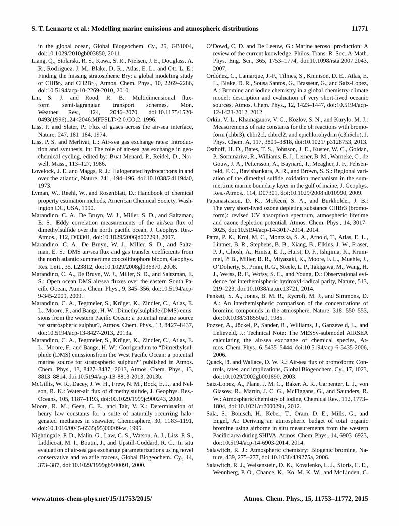
S. T. Lennartz et al.: Modelling marine emissions and atmospheric distributions 11771
in the global ocean, Global Biogeochem. Cy., 25, GB1004,
doi:10.1029/2010gb003850, 2011.
Liang, Q., Stolarski, R. S., Kawa, S. R., Nielsen, J. E., Douglass, A.
R., Rodriguez, J. M., Blake, D. R., Atlas, E. L., and Ott, L. E.:
Finding the missing stratospheric Bry: a global modeling study
of CHBr3 and CH2Br2, Atmos. Chem. Phys., 10, 2269–2286,
doi:10.5194/acp-10-2269-2010, 2010.
Lin, S. J. and Rood, R. B.: Multidimensional flux-
form semi-lagrangian transport schemes, Mon.
Weather Rev., 124, 2046–2070, doi:10.1175/1520-
0493(1996)124<2046:MFFSLT>2.0.CO;2, 1996.
Liss, P. and Slater, P.: Flux of gases across the air-sea interface,
Nature, 247, 181–184, 1974.
Liss, P. S. and Merlivat, L.: Air-sea gas exchange rates: Introduc-
tion and synthesis, in: The role of air-sea gas exchange in geo-
chemical cycling, edited by: Buat-Menard, P., Reidel, D., Nor-
well, Mass., 113–127, 1986.
Lovelock, J. E. and Maggs, R. J.: Halogenated hydrocarbons in and
over the atlantic, Nature, 241, 194–196, doi:10.1038/241194a0,
1973.
Lyman, W., Reehl, W., and Rosenblatt, D.: Handbook of chemical
property estimation mehods, American Chemical Society, Wash-
ington DC, USA, 1990.
Marandino, C. A., De Bruyn, W. J., Miller, S. D., and Saltzman,
E. S.: Eddy correlation measurements of the air/sea flux of
dimethylsulfide over the north pacific ocean, J. Geophys. Res.-
Atmos., 112, D03301, doi:10.1029/2006jd007293, 2007.
Marandino, C. A., De Bruyn, W. J., Miller, S. D., and Saltz-
man, E. S.: DMS air/sea flux and gas transfer coefficients from
the north atlantic summertime coccolithophore bloom, Geophys.
Res. Lett., 35, L23812, doi:10.1029/2008gl036370, 2008.
Marandino, C. A., De Bruyn, W. J., Miller, S. D., and Saltzman, E.
S.: Open ocean DMS air/sea fluxes over the eastern South Pa-
cific Ocean, Atmos. Chem. Phys., 9, 345–356, doi:10.5194/acp-
9-345-2009, 2009.
Marandino, C. A., Tegtmeier, S., Krüger, K., Zindler, C., Atlas, E.
L., Moore, F., and Bange, H. W.: Dimethylsulphide (DMS) emis-
sions from the western Pacific Ocean: a potential marine source
for stratospheric sulphur?, Atmos. Chem. Phys., 13, 8427–8437,
doi:10.5194/acp-13-8427-2013, 2013a.
Marandino, C. A., Tegtmeier, S., Krüger, K., Zindler, C., Atlas, E.
L., Moore, F., and Bange, H. W.: Corrigendum to “Dimethylsul-
phide (DMS) emissionsfrom the West Pacific Ocean: a potential
marine source for stratospheric sulphur?” published in Atmos.
Chem. Phys., 13, 8427–8437, 2013, Atmos. Chem. Phys., 13,
8813–8814, doi:10.5194/acp-13-8813-2013, 2013b.
McGillis, W. R., Dacey, J. W. H., Frew, N. M., Bock, E. J., and Nel-
son, R. K.: Water-air flux of dimethylsulfide, J. Geophys. Res.-
Oceans, 105, 1187–1193, doi:10.1029/1999jc900243, 2000.
Moore, R. M., Geen, C. E., and Tait, V. K.: Determination of
henry law constants for a suite of naturally-occurring halo-
genated methanes in seawater, Chemosphere, 30, 1183–1191,
doi:10.1016/0045-6535(95)00009-w, 1995.
Nightingale, P. D., Malin, G., Law, C. S., Watson, A. J., Liss, P. S.,
Liddicoat, M. I., Boutin, J., and Upstill-Goddard, R. C.: In situ
evaluation of air-sea gas exchange parameterizations using novel
conservative and volatile tracers, Global Biogeochem. Cy., 14,
373–387, doi:10.1029/1999gb900091, 2000.
O’Dowd, C. D. and De Leeuw, G.: Marine aerosol production: A
review of the current knowledge, Philos. Trans. R. Soc. A-Math.
Phys. Eng. Sci., 365, 1753–1774, doi:10.1098/rsta.2007.2043,
2007.
Ordóñez, C., Lamarque, J.-F., Tilmes, S., Kinnison, D. E., Atlas, E.
L., Blake, D. R., Sousa Santos, G., Brasseur, G., and Saiz-Lopez,
A.: Bromine and iodine chemistry in a global chemistry-climate
model: description and evaluation of very short-lived oceanic
sources, Atmos. Chem. Phys., 12, 1423–1447, doi:10.5194/acp-
12-1423-2012, 2012.
Orkin, V. L., Khamaganov, V. G., Kozlov, S. N., and Kurylo, M. J.:
Measurements of rate constants for the oh reactions with bromo-
form (chbr3), chbr2cl, chbrcl2, and epichlorohydrin (c3h5clo), J.
Phys. Chem. A, 117, 3809–3818, doi:10.1021/jp3128753, 2013.
Osthoff, H. D., Bates, T. S., Johnson, J. E., Kuster, W. C., Goldan,
P., Sommariva, R., Williams, E. J., Lerner, B. M., Warneke, C., de
Gouw, J. A., Pettersson, A., Baynard, T., Meagher, J. F., Fehsen-
feld, F. C., Ravishankara, A. R., and Brown, S. S.: Regional vari-
ation of the dimethyl sulfide oxidation mechanism in the sum-
mertime marine boundary layer in the gulf of maine, J. Geophys.
Res.-Atmos., 114, D07301, doi:10.1029/2008jd010990, 2009.
Papanastasiou, D. K., McKeen, S. A., and Burkholder, J. B.:
The very short-lived ozone depleting substance CHBr3 (bromo-
form): revised UV absorption spectrum, atmospheric lifetime
and ozone depletion potential, Atmos. Chem. Phys., 14, 3017–
3025, doi:10.5194/acp-14-3017-2014, 2014.
Patra, P. K., Krol, M. C., Montzka, S. A., Arnold, T., Atlas, E. L.,
Lintner, B. R., Stephens, B. B., Xiang, B., Elkins, J. W., Fraser,
P. J., Ghosh, A., Hintsa, E. J., Hurst, D. F., Ishijima, K., Krum-
mel, P. B., Miller, B. R., Miyazaki, K., Moore, F. L., Muehle, J.,
O’Doherty, S., Prinn, R. G., Steele, L. P., Takigawa, M., Wang, H.
J., Weiss, R. F., Wofsy, S. C., and Young, D.: Observational evi-
dence for interhemispheric hydroxyl-radical parity, Nature, 513,
219–223, doi:10.1038/nature13721, 2014.
Penkett, S. A., Jones, B. M. R., Rycroft, M. J., and Simmons, D.
A.: An interhemispheric comparison of the concentrations of
bromine compounds in the atmosphere, Nature, 318, 550–553,
doi:10.1038/318550a0, 1985.
Pozzer, A., Jöckel, P., Sander, R., Williams, J., Ganzeveld, L., and
Lelieveld, J.: Technical Note: The MESSy-submodel AIRSEA
calculating the air-sea exchange of chemical species, At-
mos. Chem. Phys., 6, 5435–5444, doi:10.5194/acp-6-5435-2006,
2006.
Quack, B. and Wallace, D. W. R.: Air-sea flux of bromoform: Con-
trols, rates, and implications, Global Biogeochem. Cy., 17, 1023,
doi:10.1029/2002gb001890, 2003.
Saiz-Lopez, A., Plane, J. M. C., Baker, A. R., Carpenter, L. J., von
Glasow, R., Martin, J. C. G., McFiggans, G., and Saunders, R.
W.: Atmospheric chemistry of iodine, Chemical Rev., 112, 1773–
1804, doi:10.1021/cr200029u, 2012.
Sala, S., Bönisch, H., Keber, T., Oram, D. E., Mills, G., and
Engel, A.: Deriving an atmospheric budget of total organic
bromine using airborne in situ measurements from the western
Pacific area during SHIVA, Atmos. Chem. Phys., 14, 6903–6923,
doi:10.5194/acp-14-6903-2014, 2014.
Salawitch, R. J.: Atmospheric chemistry: Biogenic bromine, Na-
ture, 439, 275–277, doi:10.1038/439275a, 2006.
Salawitch, R. J., Weisenstein, D. K., Kovalenko, L. J., Sioris, C. E.,
Wennberg, P. O., Chance, K., Ko, M. K. W., and McLinden, C.
www.atmos-chem-phys.net/15/11753/2015/ Atmos. Chem. Phys., 15, 11753–11772, 2015
11772 S. T. Lennartz et al.: Modelling marine emissions and atmospheric distributions
A.: Sensitivity of ozone to bromine in the lower stratosphere,
Geophys. Res. Lett., 32, L05811, doi:10.1029/2004gl021504,
2005.
Saltzman, E. S., King, D. B., Holmen, K., and Leck, C.: Exper-
imental determination of the diffusion coefficient of dimethyl-
sulfide in water, J. Geophys. Res.-Oceans, 98, 16481–16486,
doi:10.1029/93jc01858, 1993.
Sander, R., Baumgaertner, A., Gromov, S., Harder, H., Jöckel, P.,
Kerkweg, A., Kubistin, D., Regelin, E., Riede, H., Sandu, A.,
Taraborrelli, D., Tost, H., and Xie, Z.-Q.: The atmospheric chem-
istry box model CAABA/MECCA-3.0, Geosci. Model Dev., 4,
373–380, doi:10.5194/gmd-4-373-2011, 2011.
Sciare, J., Mihalopoulos, N., and Dentener, F. J.: Interannual
variability of atmospheric dimethylsulfide in the southern in-
dian ocean, J. Geophys. Res.-Atmos., 105, 26369–26377,
doi:10.1029/2000jd900236, 2000.
Sheng, J.-X., Weisenstein, D. K., Luo, B.-P., Rozanov, E., Stenke,
A., Anet, J., Bingemer, H., and Peter, T.: Global atmospheric
sulfur budget under volcanically quiescent conditions: Aerosol-
chemistry-climate model predictions and validation, J. Geophys.
Res.-Atmos., 120, 2014JD021985, doi:10.1002/2014jd021985,
2015.
Shi, Q., Petrick, G., Quack, B., Marandino, C., and Wallace, D.:
Seasonal variability of methyl iodide in the kiel fjord, J. Geo-
phys. Res.-Oceans, 119, 1609–1620, doi:10.1002/2013jc009328,
2014.
Sinnhuber, B.-M. and Meul, S.: Simulating the impact of emis-
sions of brominated very short lived substances on past strato-
spheric ozone trends, Geophys. Res. Lett., 42, 2449–2456,
doi:10.1002/2014gl062975, 2015.
Sinnhuber, B.-M., Sheode, N., Sinnhuber, M., Chipperfield, M. P.,
and Feng, W.: The contribution of anthropogenic bromine emis-
sions to past stratospheric ozone trends: a modelling study, At-
mos. Chem. Phys., 9, 2863–2871, doi:10.5194/acp-9-2863-2009,
2009.
Solomon, S., Garcia, R. R., and Ravishankara, A. R.: On the role of
iodine in ozone depletion, J. Geophys. Res.-Atmos., 99, 20491–
20499, doi:10.1029/94jd02028, 1994.
Taylor, K. E.: Summarizing multiple aspects of model performance
in a single diagram, J. Geophys. Res.-Atmos., 106, 7183–7192,
doi:10.1029/2000jd900719, 2001.
Tegtmeier, S., Krüger, K., Quack, B., Atlas, E., Blake, D. R.,
Boenisch, H., Engel, A., Hepach, H., Hossaini, R., Navarro, M.
A., Raimund, S., Sala, S., Shi, Q., and Ziska, F.: The contribution
of oceanic methyl iodide to stratospheric iodine, Atmos. Chem.
Phys., 13, 11869–11886, doi:10.5194/acp-13-11869-2013, 2013.
Tiedtke, M.: A comprehensive mass flux scheme for cu-
mulus parameterization in large-scale models, Mon.
Weather Rev., 117, 1779–1800, doi:10.1175/1520-
0493(1989)117<1779:ACMFSF>2.0.CO;2, 1989.
Tsai, W. T. and Liu, K. K.: An assessment of the effect of sea sur-
face surfactant on global atmosphere-ocean co2 flux, J. Geophys.
Res.-Oceans, 108, 3127, doi:10.1029/2000jc000740, 2003.
von Glasow, R., von Kuhlmann, R., Lawrence, M. G., Platt, U., and
Crutzen, P. J.: Impact of reactive bromine chemistry in the tropo-
sphere, Atmos. Chem. Phys., 4, 2481–2497, doi:10.5194/acp-4-
2481-2004, 2004.
Wanninkhof, R.: Relationship between wind speed and gas ex-
change over the ocean, J. Geophys. Res., 97, 7373–7382, 1992.
Wanninkhof, R. and McGillis, W. R.: A cubic relationship between
air-sea co2 exchange and wind speed, Geophys. Res. Lett., 26,
1889–1892, doi:10.1029/1999gl900363, 1999.
Wanninkhof, R., Asher, W. E., Ho, D. T., Sweeney, C., and
McGillis, W. R.: Advances in quantifying air-sea gas exchange
and environmental forcing, Ann. Rev. Marine Sci., 1, 213–244,
doi:10.1146/annurev.marine.010908.163742, 2009.
Warwick, N. J., Pyle, J. A., Carver, G. D., Yang, X., Savage, N.
H., O’Connor, F. M., and Cox, R. A.: Global modeling of bio-
genic bromocarbons, J. Geophys. Res.-Atmos., 111, D24305,
doi:10.1029/2006jd007264, 2006.
Watts, S. F.: The mass budgets of carbonyl sulfide, dimethyl sulfide,
carbon disulfide and hydrogen sulfide, Atmos. Environ., 34, 761–
779, doi:10.1016/s1352-2310(99)00342-8, 2000.
Wilke, C. R. and Chang, P.: Some measurements of diffusion in
liquids, J. Phys. Chem., 59, 592–596, 1955.
Wisher, A., Oram, D. E., Laube, J. C., Mills, G. P., van Velthoven,
P., Zahn, A., and Brenninkmeijer, C. A. M.: Very short-lived bro-
momethanes measured by the CARIBIC observatory over the
North Atlantic, Africa and Southeast Asia during 2009–2013,
Atmos. Chem. Phys., 14, 3557–3570, doi:10.5194/acp-14-3557-
2014, 2014.
Wofsy, S. C., B. C. Daube, R. Jimenez, Kort, E., Pittman, J.
V., Park, S., Commane, R., Xiang, B., Santoni, G., Jacob, D.,
Fisher, J., Pickett-Heaps, C., Wang, H., Wecht, K., Wang, Q.-Q.,
B.Stephens, B., Shertz, S., Watt, A. S., Romashkin, P., Campos,
T., Haggerty, J., Cooper, W. A., Rogers, D., Beaton, S., Hen-
dershot, R., Elkins, J. W., Fahey, D. W., Gao, R. S., Moore, F.,
Montzka, S. A., Schwarz, J. P., Perring, A. E., Hurst, D., Miller,
B. R., Sweeney, C., Oltmans, S., D.Nance, Hintsa, E., Dutton,
G., Watts, L. A., Spackman, J. R., Rosenlof, K. H., Ray, E. A.,
B. Hall, Zondlo, M. A., Diao, M., Keeling, R., Bent, J., Atlas,
E. L., Lueb, R., and Mahoney, M. J.: Hippo combined discrete
flask and gc sample ghg, halo-, hydrocarbon data (r_20121129),
Center, C. d. I. A., Oak Ridge National Laboratory, Oak Ridge,
Tenessee, USA, 2012.
Yu, S., Eder, B., Dennis, R., Chu, S.-H., and Schwartz, S. E.: New
unbiased symmetric metrics for evaluation of air quality models,
Atmos. Sci. Lett., 7, 26–34, doi:10.1002/asl.125, 2006.
Ziska, F., Quack, B., Abrahamsson, K., Archer, S. D., Atlas, E.,
Bell, T., Butler, J. H., Carpenter, L. J., Jones, C. E., Harris, N. R.
P., Hepach, H., Heumann, K. G., Hughes, C., Kuss, J., Krüger,
K., Liss, P., Moore, R. M., Orlikowska, A., Raimund, S., Reeves,
C. E., Reifenhäuser, W., Robinson, A. D., Schall, C., Tanhua,
T., Tegtmeier, S., Turner, S., Wang, L., Wallace, D., Williams, J.,
Yamamoto, H., Yvon-Lewis, S., and Yokouchi, Y.: Global sea-to-
air flux climatology for bromoform, dibromomethane and methyl
iodide, Atmos. Chem. Phys., 13, 8915–8934, doi:10.5194/acp-
13-8915-2013, 2013.
Atmos. Chem. Phys., 15, 11753–11772, 2015 www.atmos-chem-phys.net/15/11753/2015/