Embed Size (px)
Citation preview

UTMS 2005–48 December 13, 2005
Lipschitz stability in determining
density and two Lame coefficients
by
Mourad Bellassoued and Masahiro Yamamoto
UNIVERSITY OF TOKYO
GRADUATE SCHOOL OF MATHEMATICAL SCIENCES
KOMABA, TOKYO, JAPAN

LIPSCHITZ STABILITY IN DETERMINING
DENSITY AND TWO LAME COEFFICIENTS
Mourad Bellassoued1
and Masahiro Yamamoto2
1 Faculte des Sciences de Bizerte, Departement des Mathematiques,7021 Jarzouna Bizerte, Tunisia
e-mail:[email protected] Department of Mathematical Sciences, The University of Tokyo
Komaba Meguro Tokyo 153-8914 Japane-mail:[email protected] t. We consider an inverse problem of determining spatially varying density
and two Lame coefficients in a non-stationary isotropic elastic equation by a single
measuerment of data on the whole lateral boundary. We prove the Lipschitz stability
provided that initial data are suitablty chosen. The proof is based on a Carleman
estimate which can be obtained by the decomposition of the Lame system into the
rotation and the divergence components.
§1. Introduction and the main result.
We consider the three dimensional isotropic non-stationary Lame system:
ρ(x)∂2tu(x, t) − (Lλ,µu)(x, t) = f(x, t),
(x, t) ∈ Q ≡ Ω × (−T, T ), (1.1)
where
(Lλ,µv)(x) ≡ µ(x)∆v(x) + (µ(x) + λ(x))∇divv(x)
+(divv(x))∇λ(x) + (∇v + (∇v)T )∇µ(x), x ∈ Ω (1.2)
(e.g., Gurtin [12]). Throughout this paper, Ω ⊂ R3 is a bounded domain whose
boundary ∂Ω is of class C3, t and x = (x1, x2, x3) denote the time variable and the
1991 Mathematics Subject Classification. 35B60, 35R25, 35R30, 74B05.
Key words and phrases. Carleman estimate, Lame system, inverse problem.
Typeset by AMS-TEX
1
UTMS 2005–48 December 13, 2005
Lipschitz stability in determining
density and two Lame coefficients
by
Mourad Bellassoued and Masahiro Yamamoto
UNIVERSITY OF TOKYO
GRADUATE SCHOOL OF MATHEMATICAL SCIENCES
KOMABA, TOKYO, JAPAN
2 M. BELLASSOUED AND M. YAMAMOTO
spatial variable respectively, and u = (u1, u2, u3)T where ·T denotes the transpose
of matrices,
∂jφ =∂φ
∂xj, j = 1, 2, 3, ∂tφ =
∂φ
∂t.
For α = (α1, α2, α3) ∈ N∪ 03, we set ∂αx = ∂α1
1 ∂α2
2 ∂α3
3 and |α| = α1 +α2 +α3,
and ∂αx,t is similarly defined. We set ∇v = (∂kvj)1≤j,k≤3, ∇x,tv = (∇v, ∂tv)
for a vector function v = (v1, v2, v3)T . Moreover the coefficients ρ, λ, µ under
consideration, satisfy
ρ, λ, µ ∈ C2(Ω), ρ(x) > 0, µ(x) > 0, λ(x) + µ(x) > 0 for x ∈ Ω. (1.3)
Let u = u(λ, µ, ρ;p,q)(x, t) be sufficiently smooth and satisfy
ρ(x)(∂2tu)(x, t) = (Lλ,µu)(x, t), (x, t) ∈ Q, (1.4)
u(x, 0) = p(x), (∂tu)(x, 0) = q(x), x ∈ Ω. (1.5)
We consider
Inverse problem with finite measurements. Let ω ⊂ Ω be a suitable subdo-
main and let pj ,qj , 1 ≤ j ≤ N , be appropriately given. Then determine λ(x),
µ(x), ρ(x), x ∈ Ω, by
u(λ, µ, ρ;pj,qj)|ω×(−T,T ). (1.6)
As for the inverse problem of determining some (or all) of λ, µ and ρ with finite
measurements, we can first refer to:
Isakov [26] where the author proved the uniqueness in determining a single coeffi-
cient ρ(x), using four measurements (i.e., N = 4).
Ikehata, Nakamura and Yamamoto [14] which reduced the number N of measure-
ments to three for determining ρ.

INVERSE PROBLEM FOR LAME SYSTEM 3
Imanuvilov, Isakov and Yamamoto [16] which proved conditional stability and the
uniqueness in the determination of the three functions λ(x), µ(x), ρ(x), x ∈ Ω, with
two measurements (i.e., N = 2). See also Isakov [30].
Imanuvilov and Yamamoto [23] - [25] which reduced N = 2 to N = 1 (i.e., a single
measurement) in determining all of λ, µ, ρ by a single measurement u|ω×(−T,T ),
and established conditional stability of Holder type by means of an H−1-Carleman
estimate. See also [21].
As for similar inverse problems for the Lame system with residual stress, see
Isakov, Wang and Yamamoto [31], Lin and Wang [44].
Our method is based on the tool of Carleman estimates, which was originally
introduced in the field of coefficient inverse problems by Bukhgeim and Klibanov [8]
simultaneously and independently on each other for the proofs of global uniqueness
and stability theorems for these problems. Also see Klibanov [36]. In particular,
for the Lame system, we use a modification of the method in [8] by Imanuvilov
and Yamamoto [23]. In [23], only a Holder stability estimate is proved, but by the
ideas in Klibanov and Timonov [40], Klibanov and Yamamoto [41], we can prove
the Lipschitz stability for our inverse problem with N = 1. For a related technique,
see Chapter 3.5 in Klibanov and Timonov [39]. In [16] and [23], an H−1-Carleman
estimate is a key but requires more technical details. Here we will use a Carleman
estimate for the Lame system which is derived from a usual L2-Carleman estimate
for a scalar hyperbolic equation.
Thus the advantages of this paper are:
(1) the Lipschitz stability in our inverse problem with N = 1.
(2) use of a conventional Carleman estimate.

4 M. BELLASSOUED AND M. YAMAMOTO
On the other hand, for (2) we have to choose a neighbourhood ω of ∂Ω, although
it is sufficient that ω is a neighbourhood of a sufficiently large subboundary ([23]
- [25]). Then, u(λ, µ, ρ;p,q)(·, t), t ∈ (−T, T ), is given in a neighbourhood of
∂Ω, so that we do not directly assign boundary values but the observation data in
ω × (−T, T ) include information of boundary values.
For the statement of the main result, we introduce notations and an admissible
set of unknown coefficients λ, µ, ρ. Set
d = (supx∈Ω
|x− x0|2 − infx∈Ω
|x− x0|2)1
2 , (1.7)
where x0 6∈ Ω is arbitrarily fixed. Let M0 ≥ 0, 0 < θ0 ≤ 1 and θ1 > 0 be arbitrarily
fixed and let us introduce the conditions on a scalar function β:
β(x) ≥ θ1 > 0, x ∈ Ω,
‖β‖C3(Ω) ≤M0,(∇β(x) · (x− x0))
2β(x)≤ 1 − θ0, x ∈ Ω \ ω.
(1.8)
For fixed functions a(ℓ), a(ℓ)j , a
(ℓ)jk , b, bj , 1 ≤ ℓ ≤ 2, 1 ≤ j, k ≤ 3 on ∂Ω, we set
W = WM0,θ0,θ1 =
(λ, µ, ρ) ∈ C3(Ω)3;λ = a(1), ∂jλ = a
(1)j , ∂j∂kλ = a
(1)jk ,
µ = a(2), ∂jµ = a(2)j , ∂j∂kµ = a
(2)jk on ∂Ω,
λ+ 2µ
ρ,µ
ρsatisfy (1.8)
.
(1.9)
We choose θ > 0 such that
θ +M0d√θ1
√θ < θ0θ1, θ1 inf
x∈Ω|x− x0|2 − θ sup
x∈Ω|x− x0|2 > 0. (1.10)
Here we note that since x0 6∈ Ω, such θ > 0 exists.
Let E3 the 3 × 3 identity matrix. We note that (Lλ,µp)(x) is a 3-column vector
for 3-column vector p. Moreover by aj we denote the matrix (or vector) obtained
from a after deleting the j-th row and detj A means det Aj for a square matrix
A. Let (λ, µ, ρ) be an arbitrary element of W.
Now we are ready to state

INVERSE PROBLEM FOR LAME SYSTEM 5
Theorem. Let ω ⊂ Ω be a subdomain such that ∂ω ⊃ ∂Ω. For p = (p1, p2, p3)T
and q = (q1, q2, q3)T , we assume that there exist j1, j2 ∈ 1, 2, 3, 4, 5, 6 such that
detj1
((Lλ,µp)(x) (divp(x))E3 (∇p(x) + (∇p(x))T )(x− x0)(Lλ,µq)(x) (divq(x))E3 (∇q(x) + (∇q(x))T )(x− x0)
)6= 0,
∀x ∈ Ω, (1.11)
detj2
((Lλ,µp)(x) ∇p(x) + (∇p(x))T (divp)(x− x0)(Lλ,µq)(x) ∇q(x) + (∇q(x))T (divq)(x− x0)
)6= 0, ∀x ∈ Ω, (1.12)
and that
T >1√θd. (1.13)
Then, for any M1 > 0, there exists a constant C1 = C1(W,M1, ω,Ω, T, λ, µ, ρ)> 0
such that
‖λ− λ‖H2(Ω) + ‖µ− µ‖H2(Ω) + ‖ρ− ρ‖H1(Ω)
≤C1
(‖u(λ, µ, ρ;p,q)− u(λ, µ, ρ;p,q)‖H5(−T,T ;H2(ω))
+‖u(λ, µ, ρ;p,q)− u(λ, µ, ρ;p,q)‖H4(−T,T ;H
5
2 (ω))
), (1.14)
provided that (λ, µ, ρ) ∈ W and
‖u(λ, µ, ρ;p,q)‖W 7,∞(Q), ‖u(λ, µ, ρ;p,q)‖W 7,∞(Q) ≤M1. (1.15)
Inequality (1.14) gives the Lipschitz stability by a single measurement in a neigh-
bourhood of the whole boundary, and after artificial choice (1.11) and (1.12) of ini-
tial values, a single measurement yields such stability. Moreover conditions (1.11)
and (1.12) depend on a fixed (λ, µ, ρ), so that in our conclusion (1.14), we can not
change both (λ, µ, ρ), (λ, µ, ρ) ∈ W.
As the following example shows, we can take such p and q.

6 M. BELLASSOUED AND M. YAMAMOTO
Example of p, q satisfying (1.11) and (1.12). For simplicity, we assume that
λ, µ are positive constants. Noting that the fifth columns of the matrices in (1.11)
and (1.12) have x−x0 as factors, we will take quadratic functions in x. For example,
we take
p(x) =
0x1x2
0
, q(x) =
x2
2
0x2
2
.
Then, by choosing j1 = 6 and j2 = 5, we can satisfy (1.11) and (1.12).
We conclude this section with the references to other publications concerning
inverse problems by Carleman estimates after the originating paper Bukhgeim and
Klibanov [8].
(1) Baudouin and Puel [2], Bukhgeim [6] for an inverse problem of determining
potentials in Schrodinger equations,
(2) Imanuvilov and Yamamoto [17], [20], Isakov [27], [28], Klibanov [37] for the
corresponding inverse problems for parabolic equations,
(3) Amirov and Yamamoto [1], Bellassoued [3], [4], Bellassoued and Yamamoto
[5], Bukhgeim, Cheng, Isakov and Yamamoto [7], Imanuvilov and Yamamoto
[18], [19], [22] (especially for conditional stability), Isakov [27] - [29], Isakov
and Yamamoto [32], Khaıdarov [34], [35], Klibanov [36], [37], Klibanov and
Timonov [39], [40], Klibanov and Yamamoto [41], Puel and Yamamoto [45],
[46], Yamamoto [48] for inverse problems of determining potentials, damp-
ing coefficients or the principal terms in scalar hyperbolic equations.
(4) Li [42], Li and Yamamoto [43] for Maxwell’s equations.
(5) Yuan and Yamamoto [49] for plate equations.
§2. Proof of Theorem.

INVERSE PROBLEM FOR LAME SYSTEM 7
We set
ψ(x, t) = |x− x0|2 − θt2, ϕ(x, t) = eτψ(x,t), (x, t) ∈ Q
and
Qω = ω × (−T, T ).
First, in terms of (1.9) and (1.10), we can deduce the following lemma in the same
way as in [23]. Henceforth C, Cj denote constants which are independent of s but
dependent on Ω, ω, T and the choice of fixed λ, µ, ρ.
Lemma 2.1. Let (λ, µ, ρ) ∈ W and let (1.10) and (1.13) hold. There exists
τ > 0 such that for any τ > τ , we can choose s0 = s0(τ) > 0 and C1 =
C1(s0, τ0,Ω, ω, T ) > 0 such that
∫
Q
(s4|y|2 + s2|∇x,ty|2 +∑
|α|=2
|∂αxy|2
+s2|∇x,t(roty)|2 + s4|roty|2 + s2|∇x,t(divy)|2 + s4|divy|2)e2sϕdxdt
≤C1
∫
Q
(s|div f |2 + s|rot f |2 + s|f |2)e2sϕdxdt+ CeCs‖y‖2H1(−T,T ;H2(ω)), s ≥ s0
(2.1)
for any y ∈ H3(Q) such that
ρ∂2t y − Lλ,µy = f , ∂
jty(·,±T ) = 0, j = 0, 1.
The constants in (2.1) can be taken uniformly as long as (λ, µ, ρ) ∈ W.
Proof. Let us set v = divy and w = roty. Then we have (e.g., Eller, Isakov,
Nakamura and Tataru [11], Imanuvilov and Yamamoto [23]):
ρ∂2t y − µ∆y +Q1(y, v) = f in Q,
ρ∂2t v − (λ+ 2µ)∆v +Q2(y, v,w) = div f in Q
8 M. BELLASSOUED AND M. YAMAMOTO
and
ρ∂2tw − µ∆w +Q3(y, v,w) = rot f in Q,
whereQ1(y, v) =∑
|α|=1 a(1)α (x)∂αxy+
∑|α|≤1 b
(1)α (x)∂αx v, Qj(y, v,w) =
∑|α|=1 a
(j)α (x)∂αxy+
∑|α|=1 b
(j)α (x)∂αx v+
∑|α|=1 c
(j)α (x)∂αxw, j = 2, 3 and a
(j)α , b
(j)α , c
(j)α ∈ L∞(Q). There-
fore we apply a Carleman estimate by Imanuvilov [15] to the system, so that
∫
Q
s3(|roty|2 + |divy|2 + |y|2) + s(|∇x,t(roty)|2 + |∇x,t(divy)|2 + |∇x,ty|2)e2sϕdxdt
≤C∫
Q
(|div f |2 + |rot f |2 + |f |2)e2sϕdxdt+ CeCs‖y‖H1(−T,T ;H1(ω)) (2.2)
and
∫
Q
(s4|y|2 + s2|∇x,ty|2)e2sϕdxdt
≤C∫
Q
(s|div f |2 + s|rot f |2 + s|f |2)e2sϕdxdt+ CeCs‖y‖2H1(−T,T ;H1(ω)).
(2.3)
Next for all large s > 0, we have
∆(yesϕ) = ∇(div (yesϕ)) − rot (rot (yesϕ))
=3∑
j=1
∇(∂jesϕ)yj + (∂je
sϕ)∇yj + s(∇ϕ)esϕdivy + esϕ∇(divy)
+(y · ∇)(∇esϕ) − ((∇esϕ) · ∇)y
+(∇esϕ)divy − ydiv (∇esϕ) − (∇esϕ) × roty − esϕrot (roty)
=esϕ∇(divy) +O(s2)K1(y)esϕ +O(s)K2(∇y)esϕ − (rot (roty))esϕ,
where K1, K2 are linear operators. Therefore
|∆(yesϕ)| ≤ Cesϕs2|y| + s|∇y| + |∇(divy)| + |∇(roty)|,
so that
∫
Ω
|∆(y(x, t)esϕ(x,t))|2dx
≤C∫
Ω
(s4|y|2 + s2|∇y|2 + |∇(divy)|2 + |∇(roty)|2)e2sϕdx (2.4)
INVERSE PROBLEM FOR LAME SYSTEM 9
for any t ∈ [−T, T ]. The elliptic regularity and (2.4) yield
∑
|α|=2
∫
Ω
|∂αx (y(x, t)esϕ(x,t))|2dx
≤C∫
Ω
(|∆(yesϕ)|2 + |yesϕ|2)dx+ C‖yesϕ‖2
H3
2 (∂Ω)
≤C∫
Ω
(s4|y|2 + s2|∇y|2 + |∇(divy)|2 + |∇(roty)|2)e2sϕdx+ C‖yesϕ‖2H2(ω).
Therefore
∑
|α|=2
∫
Q
|(∂αxy)(x, t)esϕ(x,t)|2dxdt− Cs23∑
j=1
∫
Q
|∂jy|2e2sϕdxdt− Cs4∫
Q
|y|2e2sϕdxdt
≤C∫
Q
(s4|y|2 + s2|∇y|2 + |∇(divy)|2 + |∇(roty)|2)e2sϕdxdt
+CeCs‖y‖2L2(−T,T ;H2(ω)). (2.5)
Thus, in terms of (2.2), (2.3) and (2.5), we have
∫
Q
(s4|y|2 + s2|∇x,ty|2 +∑
|α|=2
|∂αxy|2
+s2|∇x,t(roty)|2 + s4|roty|2 + s2|∇x,t(divy)|2 + s4|divy|2)e2sϕdxdt
≤C∫
Q
(s|div f |2 + s|rot f |2 + s|f |2)e2sϕdxdt+ CeCs‖u‖2H1(−T,T ;H2(ω)).
Thus the proof of Lemma 2.1 is complete.
As for Carleman estimates, see also Hormander [13], Triggiani and Yao [47].
Next we consider a first order partial differential operator
(P0g)(x) = B(x) · ∇g(x) +B0(x)g(x), x ∈ Ω, (2.6)
where B = (b1, b2, b3) ∈ W 2,∞(Ω)3 and B0 ∈W 2,∞(Ω). Then
Lemma 2.2. We assume
|(B(x) · (x− x0))| > 0, x ∈ Ω. (2.7)

10 M. BELLASSOUED AND M. YAMAMOTO
Then there exists a constant τ0 > 0 such that for all τ > τ0, there exist s0 = s0(τ) >
0 and C2 = C2(s0, τ0,Ω, ω) > 0 such that
s2∫
Ω
∑
|α|≤2
|∂αx g(x)|2 e2sϕ(x,0)dx ≤ C2
∫
Ω
∑
|α|≤2
|∂αx (P0g)(x)|2 e2sϕ(x,0)dx
(2.8)
for all s > s0 and g ∈ C20 (Ω).
Proof of Lemma 2.2. We set F = P0g and ϕ0(x) = ϕ(x, t). By integration by
parts, we can prove
s2∫
Ω
|g|2e2sϕ0dx ≤ C2
∫
Ω
|F |2e2sϕ0dx (2.9)
(e.g., [23]). Since P0(∂jg) = ∂jF − (∂jP0)g and ∂jg|∂Ω = 0, we apply (2.9) to ∂jg,
so that
s2∫
Ω
|∂jg|2e2sϕ0dx
≤C2
∫
Ω
(|g|2 + |∇g|2)e2sϕ0dx+ C2
∫
Ω
|∂jF |2e2sϕ0dx
≤C2
∫
Ω
(|F |2 + |∂jF |2)e2sϕ0dx+ C2
∫
Ω
|∇g|2e2sϕ0dx.
Therefore
s2∫
Ω
|∇g|2e2sϕ0dx
≤C2
∫
Ω
(|F |2 + |∇F |2)e2sϕ0dx+ C2
∫
Ω
|∇g|2e2sϕ0dx.
Taking s0 > 0 sufficiently large, we have
s2∫
Ω
|∇g|2e2sϕ0dx ≤ C2
∫
Ω
(|F |2 + |∇F |2)e2sϕ0dx. (2.10)
Next we have
P0(∂k∂ℓg) = ∂k∂ℓF
−3∑
j=1
(∂kbj)(∂ℓ∂jg) + (∂ℓbj)(∂k∂jg) +K(g,∇g),

INVERSE PROBLEM FOR LAME SYSTEM 11
where K is a linear operator of g and ∇g. Noting that ∂k∂ℓg = 0 on ∂Ω, we apply
(2.9) to ∂k∂ℓg, and, similarly to (2.10), we can complete the proof of Lemma 2.2.
Finally we show an observability inequality, which may be an independent interest.
Lemma 2.3. Let (λ, µ, ρ) ∈ W and let us assume (1.13). Let u ∈ H3(Q) satisfy
(ρ∂2t − Lλ,µ)u = f . Then there exists a constant C3 > 0 such that
∫
Ω
(∑
|α|≤2
|∂αxu(x, t)|2 + |∂tu(x, t)|2)dx+
∫
Q
|∇∂tu(x, t)|2dxdt
≤C3
∫
Q
(|div f |2 + |rot f |2 + |f |2)dxdt+ C3(‖u‖2H1(−T,T ;H2(ω)) + ‖u‖2
L2(−T,T ;H5
2 (ω)))
for all t ∈ [−T, T ].
Starting from works of Klibanov and Malinsky [38] and Kazemi and Klibanov
[33], this kind of of inequality is usually proved by Carleman estimate. See e.g.,
Cheng, Isakov, Yamamoto and Zou [9], and we will prove it in Appendix for com-
pleteness.
Now we proceed to
Proof of Theorem. The proof is similar to Imanuvilov and Yamamoto [23].
Henceforth, for simplicity, we set
u = u(λ, µ, ρ;p,q), v = u(λ, µ, ρ;p,q) (2.11)
and
y = u − v, f = ρ− ρ, g = λ− λ, h = µ− µ. (2.12)
Then
ρ∂2t y = Leλ,eµ
y +Gu in Q (2.13)
and
y(x, 0) = ∂ty(x, 0) = 0, x ∈ Ω. (2.14)

12 M. BELLASSOUED AND M. YAMAMOTO
Here we set
Gu(x, t) = −f(x)∂2t u(x, t) + (g + h)(x)∇(divu)(x, t) + h(x)∆u(x, t)
+(divu)(x, t)∇g(x) + (∇u(x, t) + (∇u(x, t))T )∇h(x). (2.15)
By (1.13), we have the inequality θT 2 > d2. Therefore, by the definition of d
and the definition of the function ϕ, we have
ϕ(x, 0) ≥ d1, ϕ(x, T ) = ϕ(x,−T ) < d1, x ∈ Ω
with d1 = exp(τ infx∈Ω |x−x0|2). Thus, for given ε > 0, we can choose a sufficiently
small δ = δ(ε) > 0 such that
ϕ(x, t) ≥ d1 − ε, (x, t) ∈ Ω × [−δ, δ] (2.16)
and
ϕ(x, t) ≤ d1 − 2ε, x ∈ Ω, t ∈ [−T,−T + 2δ] ∪ [T − 2δ, T ]. (2.17)
In order to apply Lemma 2.1, it is necessary to introduce a cut-off function χ
satisfying 0 ≤ χ ≤ 1, χ ∈ C∞(R) and
χ =
0 on [−T,−T + δ] ∪ [T − δ, T ],
1 on [−T + 2δ, T − 2δ].(2.18)
In the sequel, Cj > 0 denote generic constants depending on s0, τ , M0, M1, θ0, θ1,
Ω, T , x0, ω, χ and p, q, ε, δ, but independent of s > s0.
Setting z1 = χ∂2t y, z2 = χ∂3
t y and z3 = χ∂4t y, we have
ρ∂2t z1 = Leλ,eµ
z1 + χG(∂2t u) + 2ρ(∂tχ)∂3
t y + ρ(∂2t χ)∂2
t y,
ρ∂2t z2 = Leλ,eµ
z2 + χG(∂3t u) + 2ρ(∂tχ)∂4
t y + ρ(∂2t χ)∂3
t y,
ρ∂2t z3 = Leλ,eµ
z3 + χG(∂4t u) + 2ρ(∂tχ)∂5
t y + ρ(∂2t χ)∂4
t y in Q.
(2.19)

INVERSE PROBLEM FOR LAME SYSTEM 13
We set
D = ‖y‖2H5(−T,T ;H2(ω)) + ‖y‖2
H4(−T,T ;H5
2 (ω)).
Noting that u ∈ W 7,∞(Q), in view of (2.18) and Lemma 2.1, we can Carleman
estimate (2.1) to (2.19), so that
4∑
j=2
∫
Q
(s4|∂jty|2χ2 + s2|∇∂jty|2χ2 +
∑
|α|=2
|∂αx ∂jty|2χ2
)e2sϕdxdt
≤Cs∫
Q
4∑
j=2
(χ2|∇(G(∂jtu))|2 + χ2|G(∂tu)|2)e2sϕdxdt
+Cs
∫
Q
(|∂tχ|2 + |∂2t χ|2)
5∑
j=2
(|div (∂jty)|2 + |rot (∂jty)|2 + |∂jty|2)
e2sϕdxdt
+CeCsD. (2.20)
Here we used div (ρ(∂tχ)∂jty) = ∇(ρ∂tχ)·∂jty+ρ(∂tχ)div (∂jty) and rot (ρ(∂tχ)∂jty) =
∇(ρ∂tχ) × ∂jty + ρ(∂tχ)rot (∂jty) for j = 2, 3, 4, 5.
Moreover by (1.15) we see that
|∇(G(∂jtu))| ≤ C
|∇f | + |f | +
∑
|α|≤2
|∂αx g(x)|+∑
|α|≤2
|∂αxh(x)|
in Q,
|G(∂jtu)| ≤ C(|f | + |∇g| + |∇h| + |g| + |h|) in Q (2.21)
and
|∂tχ|, |∂2t χ| 6= 0 only for t ∈ (T − 2δ, T − δ) ∪ (−T + δ,−T + 2δ). (2.22)
On the other hand, (2.13) implies
ρ∂2t (∂
jty) = Leλ,eµ
∂jty +G(∂jtu) in Q, j = 0, 1, 2, 3, 4.
14 M. BELLASSOUED AND M. YAMAMOTO
Therefore Lemma 2.3 and (2.21) yield
∫
Q
5∑
k=2
(|∇∂kt y|2 + |∂kt y|2) +
4∑
j=2
∑
|α|=2
|∂jt ∂αxy|2 dxdt
≤C4∑
j=0
(‖G(∂jtu)‖2
L2(Q) + ‖∇G(∂jtu)‖2L2(Q)
)+ CD
≤C∫
Q
∑
|α|≤2
|∂αx g(x)|2 +∑
|α|≤2
|∂αxh(x)|2 + |f(x)|2 + |∇f(x)|2 dxdt+ CD
≤C(‖f‖2H1(Ω) + ‖g‖2
H2(Ω) + ‖h‖2H2(Ω)) + CD. (2.23)
Hence inequalities (2.20), (2.21), (2.22) and (2.23) yield
4∑
j=2
∫
Q
(s4|∂jty|2χ2 + s2|∇∂jty|2χ2 +
∑
|α|=2
|∂αx∂jty|2χ2
)e2sϕdxdt
≤Cs∫
Q
|f |2 + |∇f(x)|2 +
∑
|α|≤2
|∂αx g(x)|2 +∑
|α|≤2
|∂αxh(x)|2 e2sϕdxdt
+Cse2s(d1−2ε)(‖f‖2H1(Ω) + ‖g‖2
H2(Ω) + ‖h‖2H2(Ω)) + CeCsD
≡CsE + Cs(‖f‖2H1(Ω) + ‖g‖2
H2(Ω) + ‖h‖2H2(Ω))e
2s(d1−2ε) + CeCsD.(2.24)
On the other hand, for |α| = 2, we use (2.23) and
∫
Ω
|(∂2t ∂
αxy)(x, 0)|2e2sϕ(x,0)dx
=
∫ 0
−T
∂
∂t
(∫
Ω
|(∂2t ∂
αxy)(x, t)|2χ(t)2e2sϕdx
)dt
=
∫ 0
−T
∫
Ω
2((∂3t ∂
αxy) · (∂2
t ∂αxy))χ2e2sϕdxdt
+2s
∫ 0
−T
∫
Ω
|∂2t ∂
αxy|2χ2(∂tϕ)e2sϕdxdt+
∫ 0
−T
∫
Ω
|∂2t ∂
αxy|2(∂t(χ2))e2sϕdxdt
≤C∫
Q
sχ2(|∂3t ∂
αxy|2 + |∂2
t ∂αxy|2)e2sϕdx
+Ce2s(d1−2ε)(‖f‖2H1(Ω) + ‖g‖2
H2(Ω) + ‖h‖2H2(Ω)) + CDeCs.
Therefore (2.24) yields
∑
|α|=2
∫
Ω
|(∂2t ∂
αxy)(x, 0)|2e2sϕ(x,0)dx
≤Cs2(‖f‖2H1(Ω) + ‖g‖2
H2(Ω) + ‖h‖2H2(Ω))e
2s(d1−2ε) + Cs2E + CeCsD

INVERSE PROBLEM FOR LAME SYSTEM 15
for all large s > 0. Similarly we can estimate∑
|α|=2
∫Ω|(∂3
t ∂αxy)(x, 0)|2e2sϕ(x,0)dx
to obtain
3∑
j=2
∑
|α|=2
∫
Ω
|∂αx ∂jty(x, 0)|2e2sϕ(x,0)dx
≤Cs2e2s(d1−2ε)(‖f‖2H1(Ω) + ‖g‖2
H2(Ω) + ‖h‖2H2(Ω)) + Cs2E + CeCsD
(2.25)
for all large s > 0.
Now we will consider first order partial differential equations satisfied by h, g
and f . That is, by (2.13), (2.14) and (1.15), we have
ρ∂2t y(x, 0) = Gu(x, 0), ρ∂3
t y(x, 0) = G∂tu(x, 0). (2.26)
For simplicity, we set
a =
(− 1ρLλ,µp
− 1ρLλ,µq
),
b1 =
divp00
divq00
, b2 =
0divp
00
divq0
, b3 =
00
divp00
divq
,
(d1,d2,d3) =
(∇p + (∇p)T
∇q + (∇q)T
),
G =
(ρ∂2t y(x, 0) − (g + h)∇(divp) − h∆p
ρ∂3t y(x, 0) − (g + h)∇(divq) − h∆q
)on Ω.
(2.27)
Then we can rewrite (2.26) as
af + b1∂1g + b2∂2g + b3∂3g = G− d1∂1h− d2∂2h− d3∂3h.
Therefore for j1 ∈ 1, 2, 3, 4, 5, 6, we have
aj1f + b1j1∂1g + b2j1∂2g + b3j1∂3g
=Gj1 − d1j1∂1h− d2j1∂2h− d3j1∂3h on Ω. (2.28)

16 M. BELLASSOUED AND M. YAMAMOTO
Equality (2.28) is a system of five linear equations with respect to four unknowns
f , ∂1g, ∂2g, ∂3g, and so for the existence of solutions, we need the consistency of
the coefficients, that is,
detj1 (a,b1,b2,b3,G− d1∂1h− d2∂2h− d3∂3h) = 0 on Ω,
that is,
3∑
k=1
detj1 (a,b1,b2,b3,dk)∂kh = detj1 (a,b1,b2,b3,G) on Ω (2.29)
by the linearity of the determinant. Here by (1.15) we note that p,q ∈ W 5,∞(Ω)
and
∑
|α|≤2
|∂αxG(x)| ≤ C
3∑
j=2
∑
|α|≤2
|∂αx ∂jty(x, 0)|
+C∑
|α|≤2
|∂αx g(x)|+ C∑
|α|≤2
|∂αxh(x)|.
In terms of condition (1.11) and h ≡ µ− µ ∈ C20 (Ω), considering (2.29) as a first
order partial differential operator in h, we can apply Lemma 2.2 to obtain
s2∫
Ω
∑
|α|≤2
|∂αxh|2e2sϕ(x,0)dx ≤ C
∫
Ω
3∑
j=2
∑
|α|≤2
|∂αx ∂jty(x, 0)|2e2sϕ(x,0)dx
+C
∫
Ω
∑
|α|≤2
|∂αx g(x)|2 +∑
|α|≤2
|∂αxh(x)|2 e2sϕ(x,0)dx
≤Cs2e2s(d1−2ε)(‖f‖2H1(Ω) + ‖g‖2
H2(Ω) + ‖h‖2H2(Ω)) + Cs2E + CeCsD
+C
∫
Ω
∑
|α|≤2
|∂αx g(x)|2 +∑
|α|≤2
|∂αxh(x)|2 e2sϕ(x,0)dx (2.30)
for all large s > 0. Here we used (2.25). Similarly to (2.30), in terms of (1.12), we

INVERSE PROBLEM FOR LAME SYSTEM 17
can argue for g. Hence with (2.30), we have
∫
Ω
∑
|α|≤2
|∂αx g(x)|2 +∑
|α|≤2
|∂αxh(x)|2 e2sϕ(x,0)dx
≤Ce2s(d1−2ε)(‖f‖2H1(Ω) + ‖g‖2
H2(Ω) + ‖h‖2H2(Ω))
+C
∫
Q
|f(x)|2 + |∇f(x)|2 +
∑
|α|≤2
|∂αx g(x)|2 +∑
|α|≤2
|∂αxh(x)|2 e2sϕdxdt+ CeCsD
+C
s2
∫
Ω
∑
|α|≤2
|∂αx g(x)|2 +∑
|α|≤2
|∂αxh(x)|2 e2sϕ(x,0)dx
for all large s > 0. Here we recall the definition of E in (2.24). Taking s > 0
sufficiently large, we can absorb the last term into the left hand side:
∫
Ω
∑
|α|≤2
|∂αx g(x)|2 +∑
|α|≤2
|∂αxh(x)|2 e2sϕ(x,0)dx
≤Ce2s(d1−2ε)(‖f‖2H1(Ω) + ‖g‖2
H2(Ω) + ‖h‖2H2(Ω))
+C
∫
Q
|f(x)|2 + |∇f(x)|2 +
∑
|α|≤2
|∂αx g(x)|2 +∑
|α|≤2
|∂αxh(x)|2 e2sϕdxdt+ CeCsD.
(2.31)
Finally, by (2.28), we have
af = −b1∂1g − b2∂2g − b3∂3g + G− d1∂1h− d2∂2h− d3∂3h in Ω.
Moreover, by (1.11) or (1.12), we see that |a(x)| > 0 for x ∈ Ω, so that
f(x) = K1G + K2(∇g,∇h) in Ω,
where K1, K2 are linear operators with W 1,∞-coefficients. Thus
|∇f(x)| ≤ C
|∇G(x)| +
∑
|α|≤2
|∂αx g(x)| +∑
|α|≤2
|∂αxh(x)|
≤C
3∑
j=2
(|∇(∂jty)(x, 0)|+ |∂jty(x, 0)|) +∑
|α|≤2
|∂αx g(x)|+∑
|α|≤2
|∂αxh(x)|
,
and
|f(x)| ≤ C
3∑
j=2
|∂jty(x, 0)| +∑
|α|≤2
|∂αx g(x)|+∑
|α|≤2
|∂αxh(x)|
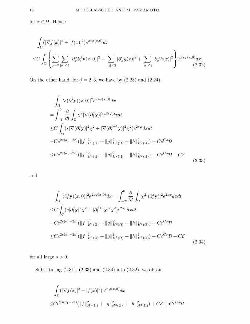
18 M. BELLASSOUED AND M. YAMAMOTO
for x ∈ Ω. Hence
∫
Ω
(|∇f(x)|2 + |f(x)|2)e2sϕ(x,0)dx
≤C∫
Ω
3∑
j=2
∑
|α|≤1
|∂αx∂jty(x, 0)|2 +∑
|α|≤2
|∂αx g(x)|2 +∑
|α|≤2
|∂αxh(x)|2 e2sϕ(x,0)dx.
(2.32)
On the other hand, for j = 2, 3, we have by (2.23) and (2.24),
∫
Ω
|∇(∂jty)(x, 0)|2e2sϕ(x,0)dx
=
∫ 0
−T
∂
∂t
∫
Ω
χ2|∇(∂jty)|2e2sϕdxdt
≤C∫
Q
(s|∇(∂jty)|2χ2 + |∇(∂j+1t y)|2χ2)e2sϕdxdt
+Ce2s(d1−2ε)(‖f‖2H1(Ω) + ‖g‖2
H2(Ω) + ‖h‖2H2(Ω)) + CeCsD
≤Ce2s(d1−2ε)(‖f‖2H1(Ω) + ‖g‖2
H2(Ω) + ‖h‖2H2(Ω)) + CeCsD + CE
(2.33)
and
∫
Ω
|(∂jty)(x, 0)|2e2sϕ(x,0)dx =
∫ 0
−T
∂
∂t
∫
Ω
χ2|(∂jty)|2e2sϕdxdt
≤C∫
Q
(s|∂jty|2χ2 + |∂j+1t y|2χ2)e2sϕdxdt
+Ce2s(d1−2ε)(‖f‖2H1(Ω) + ‖g‖2
H2(Ω) + ‖h‖2H2(Ω)) + CeCsD
≤Ce2s(d1−2ε)(‖f‖2H1(Ω) + ‖g‖2
H2(Ω) + ‖h‖2H2(Ω)) + CeCsD + CE
(2.34)
for all large s > 0.
Substituting (2.31), (2.33) and (2.34) into (2.32), we obtain
∫
Ω
(|∇f(x)|2 + |f(x)|2)e2sϕ(x,0)dx
≤Ce2s(d1−2ε)(‖f‖2H1(Ω) + ‖g‖2
H2(Ω) + ‖h‖2H2(Ω)) + CE + CeCsD.

INVERSE PROBLEM FOR LAME SYSTEM 19
Here with (2.31), we have
∫
Ω
∑
|α|≤2
|∂αx g|2 +∑
|α|≤2
|∂αxh|2 + |∇f |2 + |f |2 e2sϕ(x,0)dx
≤Ce2s(d1−2ε)(‖f‖2H1(Ω) + ‖g‖2
H2(Ω) + ‖h‖2H2(Ω)) + CeCsD
+C
∫
Q
∑
|α|≤2
|∂αx g|2 +∑
|α|≤2
|∂αxh|2 + |∇f |2 + |f |2 e2sϕdxdt.
Since
∫
Q
∑
|α|≤2
|∂αx g|2 +∑
|α|≤2
|∂αxh|2 + |∇f |2 + |f |2 e2sϕdxdt
=
∫
Ω
∑
|α|≤2
|∂αx g|2 +∑
|α|≤2
|∂αxh|2 + |∇f |2 + |f |2 e2sϕ(x,0)
(∫ T
−T
e2s(ϕ(x,t)−ϕ(x,0))dt
)dx
=o(1)
∫
Ω
∑
|α|≤2
|∂αx g|2 +∑
|α|≤2
|∂αxh|2 + |∇f |2 + |f |2 e2sϕ(x,0)dx,
as s −→ ∞ by the Lebesgue theorem and ϕ(x, t) < ϕ(x, 0) for t 6= 0, we can absorb
the last term at the right hand side into the left hand side, and
∫
Ω
∑
|α|≤2
|∂αx g|2 +∑
|α|≤2
|∂αxh|2 + |∇f |2 + |f |2 e2sϕ(x,0)dx
≤Ce2s(d1−2ε)(‖f‖2H1(Ω) + ‖g‖2
H2(Ω) + ‖h‖2H2(Ω)) + CeCsD
for all large s > 0. By ϕ(x, 0) ≥ d1, we divide the both sides by e2sd1 , we have
∫
Ω
∑
|α|≤2
|∂αx g|2 +∑
|α|≤2
|∂αxh|2 + |∇f |2 + |f |2 dx
≤Ce−4sε(‖f‖2H1(Ω) + ‖g‖2
H2(Ω) + ‖h‖2H2(Ω)) + CeCsD
for all large s > 0. Choosing s > 0 sufficiently large, we can absorb the first term
at the right hand side into the left hand side, so that we have conclusion (1.14).
Appendix. Proof of Lemma 2.3.
Let us set v = divu and w = rotu. Then, as in the proof of Lemma 2.1, we have
ρ∂2t u − µ∆u +Q1(u, v) = f in Q, (1)

20 M. BELLASSOUED AND M. YAMAMOTO
ρ∂2t v − (λ+ 2µ)∆v +Q2(u, v,w) = div f in Q (2)
and
ρ∂2tw − µ∆w +Q3(u, v,w) = rot f in Q, (3)
whereQ1(u, v) =∑
|α|=1 a(1)α (x)∂αxu+
∑|α|≤1 b
(1)α (x)∂αx v, Qj(u, v,w) =
∑|α|=1 a
(j)α (x)∂αxu+
∑|α|=1 b
(j)α (x)∂αx v +
∑|α|=1 c
(j)α (x)∂αxw, j = 2, 3 and a
(j)α , b
(j)α , c
(j)α ∈ L∞(Q).
Let t ≥ 0. We set
E1(t) ≡∫
Ω
(|∇x,tu(x, t)|2 + |∇x,tv(x, t)|2 + |∇x,tw(x, t)|2)dx.
Taking the scalar products of (1) and (3) with ∂tu and ∂tw respectively and mul-
tiplying (2) with ∂tv, we integrate by parts to have
E1(t) ≤ CE1(0) + C
(∫ t
0
E1(ξ)dξ + ‖f‖2L2(Q) + ‖div f‖2
L2(Q) + ‖rot f‖2L2(Q)
)
+C(‖∂tu‖2L2(∂Ω×(−T,T )) + ‖∂νu‖2
L2(∂Ω×(−T,T )) + ‖∂tv‖2L2(∂Ω×(−T,T )) + ‖∂νv‖2
L2(∂Ω×(−T,T ))
+‖∂tw‖2L2(∂Ω×(−T,T )) + ‖∂νw‖2
L2(∂Ω×(−T,T ))).
Applying the trace theorem, we have
E1(t) ≤ CE1(0) + CF + C
∫ t
0
E1(ξ)dξ, 0 ≤ t ≤ T.
Here we set
F = ‖u‖2H1(−T,T ;H2(ω))+‖u‖2
L2(−T,T ;H5
2 (ω))+‖div f‖2
L2(Q)+‖rot f‖2L2(Q)+‖f‖2
L2(Q).
The Gronwall inequality implies E1(t) ≤ C(F + E1(0)), 0 ≤ t ≤ T . Similarly we
can prove C−1E1(0) ≤ E1(t) + CF , 0 ≤ t ≤ T . For −T ≤ t ≤ 0, we can simiarly
argue to obtain
E1(t1) ≤ CE1(t2) + CF, −T ≤ t1, t2 ≤ T. (4)
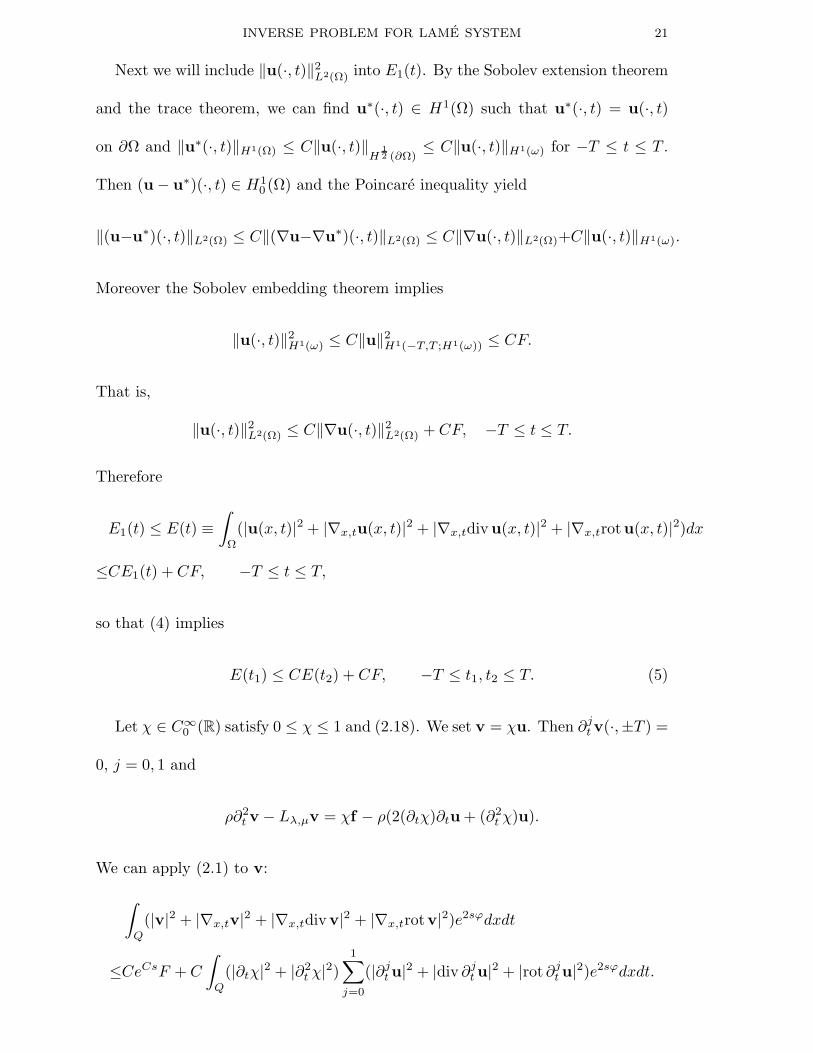
INVERSE PROBLEM FOR LAME SYSTEM 21
Next we will include ‖u(·, t)‖2L2(Ω) into E1(t). By the Sobolev extension theorem
and the trace theorem, we can find u∗(·, t) ∈ H1(Ω) such that u∗(·, t) = u(·, t)
on ∂Ω and ‖u∗(·, t)‖H1(Ω) ≤ C‖u(·, t)‖H
1
2 (∂Ω)≤ C‖u(·, t)‖H1(ω) for −T ≤ t ≤ T .
Then (u − u∗)(·, t) ∈ H10 (Ω) and the Poincare inequality yield
‖(u−u∗)(·, t)‖L2(Ω) ≤ C‖(∇u−∇u∗)(·, t)‖L2(Ω) ≤ C‖∇u(·, t)‖L2(Ω)+C‖u(·, t)‖H1(ω).
Moreover the Sobolev embedding theorem implies
‖u(·, t)‖2H1(ω) ≤ C‖u‖2
H1(−T,T ;H1(ω)) ≤ CF.
That is,
‖u(·, t)‖2L2(Ω) ≤ C‖∇u(·, t)‖2
L2(Ω) + CF, −T ≤ t ≤ T.
Therefore
E1(t) ≤ E(t) ≡∫
Ω
(|u(x, t)|2 + |∇x,tu(x, t)|2 + |∇x,tdivu(x, t)|2 + |∇x,trotu(x, t)|2)dx
≤CE1(t) + CF, −T ≤ t ≤ T,
so that (4) implies
E(t1) ≤ CE(t2) + CF, −T ≤ t1, t2 ≤ T. (5)
Let χ ∈ C∞0 (R) satisfy 0 ≤ χ ≤ 1 and (2.18). We set v = χu. Then ∂jtv(·,±T ) =
0, j = 0, 1 and
ρ∂2t v − Lλ,µv = χf − ρ(2(∂tχ)∂tu + (∂2
t χ)u).
We can apply (2.1) to v:
∫
Q
(|v|2 + |∇x,tv|2 + |∇x,tdivv|2 + |∇x,trotv|2)e2sϕdxdt
≤CeCsF + C
∫
Q
(|∂tχ|2 + |∂2t χ|2)
1∑
j=0
(|∂jtu|2 + |div ∂jtu|2 + |rot ∂jtu|2)e2sϕdxdt.
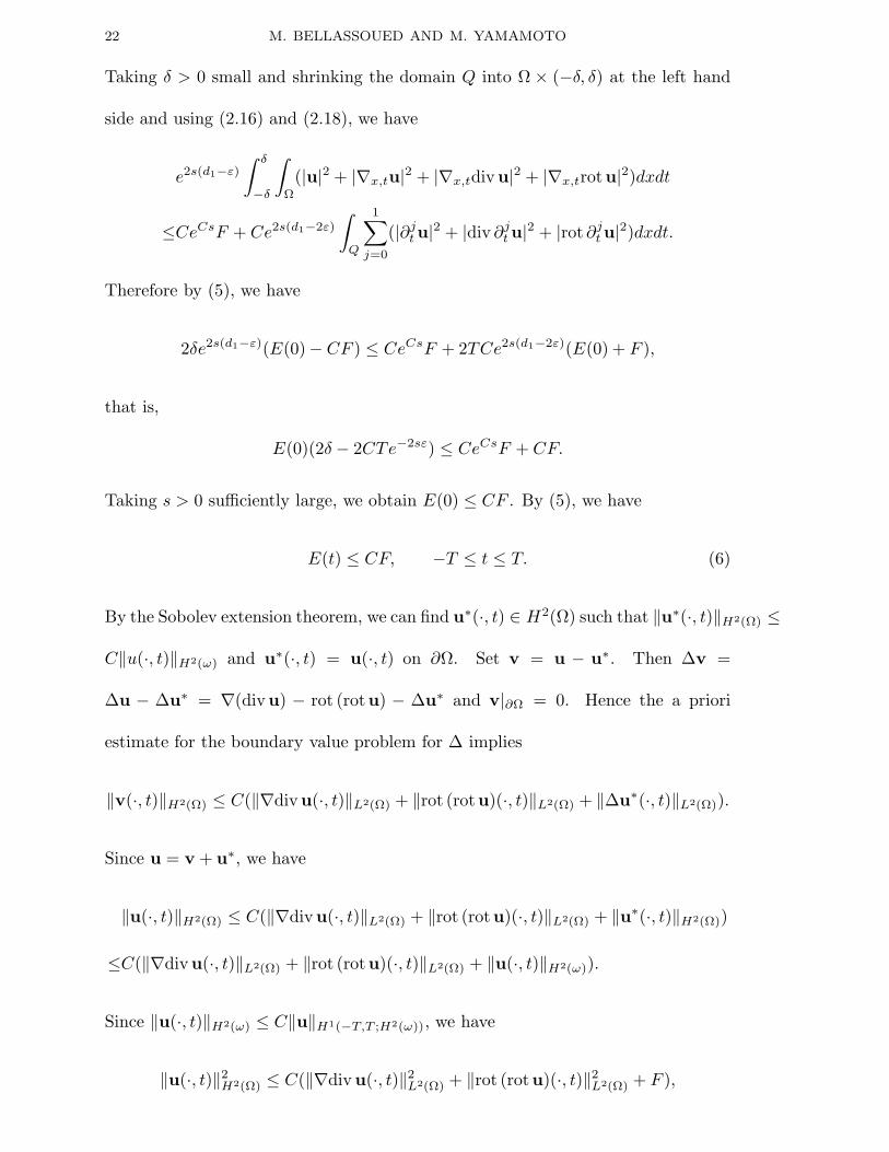
22 M. BELLASSOUED AND M. YAMAMOTO
Taking δ > 0 small and shrinking the domain Q into Ω × (−δ, δ) at the left hand
side and using (2.16) and (2.18), we have
e2s(d1−ε)∫ δ
−δ
∫
Ω
(|u|2 + |∇x,tu|2 + |∇x,tdivu|2 + |∇x,trotu|2)dxdt
≤CeCsF + Ce2s(d1−2ε)
∫
Q
1∑
j=0
(|∂jtu|2 + |div ∂jtu|2 + |rot ∂jtu|2)dxdt.
Therefore by (5), we have
2δe2s(d1−ε)(E(0)− CF ) ≤ CeCsF + 2TCe2s(d1−2ε)(E(0) + F ),
that is,
E(0)(2δ − 2CTe−2sε) ≤ CeCsF + CF.
Taking s > 0 sufficiently large, we obtain E(0) ≤ CF . By (5), we have
E(t) ≤ CF, −T ≤ t ≤ T. (6)
By the Sobolev extension theorem, we can find u∗(·, t) ∈ H2(Ω) such that ‖u∗(·, t)‖H2(Ω) ≤
C‖u(·, t)‖H2(ω) and u∗(·, t) = u(·, t) on ∂Ω. Set v = u − u∗. Then ∆v =
∆u − ∆u∗ = ∇(divu) − rot (rotu) − ∆u∗ and v|∂Ω = 0. Hence the a priori
estimate for the boundary value problem for ∆ implies
‖v(·, t)‖H2(Ω) ≤ C(‖∇divu(·, t)‖L2(Ω) + ‖rot (rotu)(·, t)‖L2(Ω) + ‖∆u∗(·, t)‖L2(Ω)).
Since u = v + u∗, we have
‖u(·, t)‖H2(Ω) ≤ C(‖∇divu(·, t)‖L2(Ω) + ‖rot (rotu)(·, t)‖L2(Ω) + ‖u∗(·, t)‖H2(Ω))
≤C(‖∇divu(·, t)‖L2(Ω) + ‖rot (rotu)(·, t)‖L2(Ω) + ‖u(·, t)‖H2(ω)).
Since ‖u(·, t)‖H2(ω) ≤ C‖u‖H1(−T,T ;H2(ω)), we have
‖u(·, t)‖2H2(Ω) ≤ C(‖∇divu(·, t)‖2
L2(Ω) + ‖rot (rotu)(·, t)‖2L2(Ω) + F ),

INVERSE PROBLEM FOR LAME SYSTEM 23
with which (6) yields
∫
Ω
∑
|α|≤2
|∂αxu(x, t)|2 + |∂tu(x, t)|2 + |∂tdivu(x, t)|2 + |∂trotu(x, t)|2 dx ≤ CF.
(7)
Finally we will estimate ∇(∂tu) at the right hand side of the conclusion. By the
Sobolev extension theorem and the trace theorem, for −T ≤ t ≤ T we can find
u∗1 such that u∗
1(·, t) = ∂tu(·, t) on ∂Ω and ‖u∗1(·, t)‖H1(Ω) ≤ C‖∂tu(·, t)‖
H1
2 (∂Ω)≤
C‖∂tu(·, t)‖H1(ω). Applying Theorem 6.1 (pp.358-359) in Duvaut and Lions [10],
we have
‖∂tu(·, t)− u∗1(·, t)‖H1(Ω) ≤ C‖∂tu(·, t)− u∗
1(·, t)‖L2(Ω)
+C‖div (∂tu(·, t) − u∗1(·, t))‖L2(Ω) + C‖rot (∂tu(·, t)− u∗
1(·, t))‖L2(Ω),
that is,
∫
Ω
|∂t∇u(x, t)|2dx
≤C∫
Ω
(|∂tu(x, t)|2 + |∂tdivu(x, t)|2 + |∂trotu(x, t)|2)dx+ C‖∂tu(·, t)‖2H1(ω).
Hence by (7), we obtain
∫
Q
|∂t∇u|2dxdt
≤C∫
Q
(|∂tu(x, t)|2 + |∂tdivu(x, t)|2 + |∂trotu(x, t)|2)dxdt+ CF ≤ CF.
(8)
Inequality (7) and (8) completes the proof of Lemma 2.3.
Acknowledgements. Most ot this paper has been written during the stays of the
first named author at Graduate School of Mathematical Sciences of the University
of Tokyo. The first named authors thanks the school for the hospitality. The second
named author was partly supported by Grant 15340027 from the Japan Society for
the Promotion of Science and Grant 17654019 from the Ministry of Education,
Cultures, Sports and Technology.

24 M. BELLASSOUED AND M. YAMAMOTO
References
1. A. Amirov and M. Yamamoto, Unique continuation and an inverse problemfor hyperbolic equations across a general hypersurface, J. Phys.: Conf. Ser. 12(2005), 1-12.
2. L. Baudouin and J.-P. Puel, Uniqueness and stability in an inverse problem forthe Schrodinger equation, Inverse Problems 18 (2002), 1537 – 1554.
3. M. Bellassoued, Uniqueness and stability in determining the speed of propaga-tion of second-order hyperbolic equation with variable coefficients, Appl. Anal.83 (2004), 983–1014.
4. M. Bellassoued, Global logarithmic stability in inverse hyperbolic problem byarbitrary boundary observation, Inverse Problems 20 (2004), 1033-1052.
5. M. Bellassoued and M. Yamamoto, Logarithmic stability in determination of acoefficient in an acoustic equation by arbitrary boundary observation, to appearin J. Math. Pures Appl.
6. A.L. Bukhgeim, Introduction to the Theory of Inverse Problems, VSP, Utrecht,2000.
7. A.L. Bukhgeim, J. Cheng, V. Isakov and M. Yamamoto, Uniqueness in de-termining damping coefficients in hyperbolic equations, in ”Analytic ExtensionFormulas and their Applications” (2001), Kluwer, Dordrecht, 27-46.
8. A.L. Bukhgeim and M.V. Klibanov, Global uniqueness of a class of multidi-mensional inverse problems, Soviet Math. Dokl. 24 (1981), 244–247.
9. J. Cheng, V. Isakov, M. Yamamoto and Q. Zhou, Lipschitz stability in thelateral Cauchy problem for elasticity system, J. Math. Kyoto Univ. 43 (2003),475–501.
10. G. Duvaut and J.L. Lions, Inequalities in Mechanics and Physics, Springer-Verlag, Berlin, 1976.
11. M. Eller, V. Isakov, G. Nakamura and D.Tataru, Uniqueness and stability in theCauchy problem for Maxwell’s and the elasticity systems, in ”Nonlinear PartialDifferential Equations”, Vol.14, College de France Seminar, Elsevier-GauthierVillars (2002), 329–350.
12. M.E. Gurtin, The Linear Theory of Elasticity, in ”Encyclopedia of Physics”Volume VIa/2, Mechanis of Solids II, C. Truesdell, ed., Springer-Verlag, Berlin,1972.
13. L. Hormander, Linear Partial Differential Operators, Springer-Verlag, Berlin,1963.
14. M. Ikehata, G. Nakamura and M. Yamamoto, Uniqueness in inverse problemsfor the isotropic Lame system, J. Math. Sci. Univ. Tokyo 5 (1998), 627–692.
15. O. Imanuvilov, On Carleman estimates for hyperbolic equations, AsymptoticAnalysis 32 (2002), 185–220.
16. O. Imanuvilov, V. Isakov and M. Yamamoto, An inverse problem for the dy-namical Lame system with two sets of boundary data, Comm. Pure Appl. Math56 (2003), 1366–1382.
17. O. Imanuvilov and M. Yamamoto, Lipschitz stability in inverse parabolic prob-lems by the Carleman estimate, Inverse Problems 14 (1998), 1229–1245.
18. O. Imanuvilov and M. Yamamoto, Global Lipschitz stability in an inverse hy-perbolic problem by interior observations, Inverse Problems 17 (2001), 717–728.
19. O. Imanuvilov and M. Yamamoto, Global uniqueness and stability in determin-ing coefficients of wave equations, Commun. in Partial Differential Equations
INVERSE PROBLEM FOR LAME SYSTEM 25
26 (2001), 1409–1425.
20. O. Imanuvilov and M. Yamamoto, Carleman estimate for a parabolic equa-tion in a Sobolev space of negative order and its applications, in ”Control ofNonlinear Distributed Parameter Systems” (2001), Marcel Dekker, New York,113–137.
21. O. Imanuvilov and M. Yamamoto, Remarks on Carleman estimates and con-trollability for the Lame system, Journees ”Equations aux Derivees Partielles”,Forges-les-Eaux, 3-7 juin 2002, GDR 2434 (CNRS), V-1-V-19.
22. O. Imanuvilov and M. Yamamoto, Determination of a coefficient in an acousticequation with a single measurement, Inverse Problems 19 (2003), 151–171.
23. O. Imanuvilov and M. Yamamoto, Carleman estimates for the non-stationaryLame system and the application to an inverse problem, ESAIM Control Optim.Calc. Var. 11, no.1 (2005), 1–56 (electronic).
24. O. Imanuvilov and M. Yamamoto, Carleman estimates for the three-dimensionalnonstationary Lame system and application to an inverse problem, in ”ControlTheory of Parital Differential Equations” (2005), Chapman & Hall/CRC, BocaRaton, 337–374.
25. O. Imanuvilov and M. Yamamoto, Carleman estimates for the Lame sys-tem with stress boundary condition and the application to an inverse problem,Preprint No. 2004-02, Department of Mathematical Sciences of The Univer-sity of Tokyo, also available at http://kyokan.ms.u-tokyo.ac.jp/users/preprint/preprint2004.html.
26. V. Isakov, A nonhyperbolic Cauchy problem for bc and its applications toelasticity theory, Comm. Pure and Applied Math. 39 (1986), 747–767.
27. V. Isakov, Inverse Source Problems, American Mathematical Society, Provi-dence, Rhode Island, 1990.
28. V. Isakov, Inverse Problems for Partial Differential Equations, Springer-Verlag,Berlin, 1998.
29. V. Isakov, Carleman type estimates and their applications, in ”New Analyticand Geometric Methods in Inverse Problems” (2004), Springer-Verlag, Berlin,93–125.
30. V. Isakov An inverse problem for the dynamical Lame system with two setsof local boundary data, in ”Control Theory of Parital Differential Equations”(2005), Chapman & Hall/CRC, Boca Raton, 101–110.
31. V. Isakov, J.-N. Wang and M. Yamamoto, Uniqueness and stability of deter-mining the residual stress by one measurement, preprint.
32. V. Isakov and M. Yamamoto, Carleman estimate with the Neumann bound-ary condition and its applications to the observability inequality and inversehyperbolic problems, Contem. Math. 268 (2000), 191–225.
33. M.A. Kazemi and M.V. Klibanov, Stability estimates for ill-posed Cauchy prob-lems involving hyperbolic equations and inequalities, Appl. Anal. 50 (1993),93-102.
34. A. Khaıdarov, Carleman estimates and inverse problems for second order hy-perbolic equations, Math. USSR Sbornik 58 (1987), 267-277.
35. A. Khaıdarov, On stability estimates in multidimensional inverse problems fordifferential equations, SovietMath.Dokl. 38 (1989), 614-617.
36. M.V. Klibanov, Inverse problems in the ”large” and Carleman bounds, Differ-ential Equations 20 (1984), 755-760.

26 M. BELLASSOUED AND M. YAMAMOTO
37. M.V. Klibanov, Inverse problems and Carleman estimates, Inverse Problems 8(1992), 575–596.
38. M.V. Klibanov and J. Malinsky, Newton-Kantorovich method for 3-dimensionalpotential inverse scattering problem and stability of the hyperbolic Cauchy prob-lem with time dependent data, Inverse Problems 7 (1992), 577–595.
39. M.V. Klibanov and A. Timonov, Carleman Estimates for Coefficient InverseProblems and Numerical Applications, VSP, Utrecht, 2004.
40. M.V. Klibanov and A. Timonov, Global uniqueness for a 3d/2d inverse con-ductivity problem via the modified method of Carleman estimtes, J. Inverse andIll-Posed Problems 13 (2005), 149-174.
41. M.V. Klibanov and M. Yamamoto, Lipschitz stability of an inverse problem foran accoustic equation, to appear in Applicable Analysis, 2005.
42. S. Li, An inverse problem for Maxwell’s equations in biisotropic media, toappear in SIAM J. Math. Anal.
43. S. Li and M. Yamamoto, Carleman estimate for Maxwell’s equations in anisotropicmedia and the observability inequality, J. Phys.: Conf. Ser. 12 (2005), 110-115.
44. C.-L. Lin and J.-N. Wang, Uniqueness in inverse problems for an elasticitysystem with residual stress, Inverse Problems 19 (2003), 807-820.
45. J.-P. Puel and M. Yamamoto, On a global estimate in a linear inverse hyperbolicproblem, Inverse Problems 12 (1996), 995-1002.
46. J.-P. Puel and M. Yamamoto, Generic well-posedness in a multidimensionalhyperbolic inverse problem, J. Inverse Ill-posed Problems 5 (1997), 55–83.
47. R.Triggiani and P.F.Yao, Carleman estimates with no lower-order terms forgeneral Riemann wave equation. global uniqueness and observability in oneshot, Appl. Math. Optim. 46 (2002), 331-375.
48. M. Yamamoto, Uniqueness and stability in multidimensional hyperbolic inverseproblems, J. Math. Pures Appl. 78 (1999), 65–98.
49. G. Yuan and M. Yamamoto, Lipschitz stability in inverse problems for a Kirch-hoff plate equation, Preprint No. 2005-36, The Department of MathematicalSciences of The University of Tokyo, also available at http://kyokan.ms.u-tokyo.ac.jp/users/preprint /preprint2005.html.

Preprint Series, Graduate School of Mathematical Sciences, The University of Tokyo
UTMS
2005–38 Noriaki Umeda: Existence and nonexistence of global solutions of a weaklycoupled system of reaction-diffusion equations.
2005–39 Yuji Morimoto: Homogeneous coherent value measures and their limits undermultiperiod collective risk processes.
2005–40 X. Q. Wan, Y. B. Wang, and M. Yamamoto: The local property of the regular-ized solutions in numerical differentiation.
2005–41 Yoshihiro Sawano: lq-valued extension of the fractional maximal operators fornon-doubling measures via potential operators .
2005–42 Yuuki Tadokoro: The pointed harmonic volumes of hyperelliptic curves withWeierstrass base points.
2005–43 X. Q. Wan, Y. B. Wang and M. Yamamoto: Detection of irregular points byregularization in numerical differentiation and an application to edge detection.
2005–44 Victor Isakov, Jenn-Nan Wang and Masahiro Yamamoto: Uniqueness andstability of determining the residual stress by one measurement.
2005–45 Yoshihiro Sawano and Hitoshi Tanaka: The John-Nirenberg type inequality fornon-doubling measures.
2005–46 Li Shumin and Masahiro Yamamoto: An inverse problem for Maxwell’s equa-tions in anisotropic media.
2005–47 Li Shumin: Estimation of coefficients in a hyperbolic equation with impulsiveinputs.
2005–48 Mourad Bellassoued and Masahiro Yamamoto: Lipschitz stability in determin-ing density and two Lame coefficients.
The Graduate School of Mathematical Sciences was established in the University ofTokyo in April, 1992. Formerly there were two departments of mathematics in the Uni-versity of Tokyo: one in the Faculty of Science and the other in the College of Arts andSciences. All faculty members of these two departments have moved to the new gradu-ate school, as well as several members of the Department of Pure and Applied Sciencesin the College of Arts and Sciences. In January, 1993, the preprint series of the formertwo departments of mathematics were unified as the Preprint Series of the GraduateSchool of Mathematical Sciences, The University of Tokyo. For the information aboutthe preprint series, please write to the preprint series office.
ADDRESS:Graduate School of Mathematical Sciences, The University of Tokyo3–8–1 Komaba Meguro-ku, Tokyo 153-8914, JAPANTEL +81-3-5465-7001 FAX +81-3-5465-7012