Embed Size (px)
Citation preview

Dissertation
submitted to the
Combined Faculties for the Natural Sciences and for Mathematics
of the Ruperto-Carola University of Heidelberg, Germany
for the degree of
Doctor of Natural Sciences
Put forward by
M.Sc. Olga Zacharopoulou
born in Athens, Greece
oral examination: 13.12.2010


On the Origin of the Unusually Hard
γ-ray Spectra of TeV Blazars
Referees:
Prof. Dr. Felix Aharonian
PD Dr. Christian Fendt


to my grandmother

AbstractThe observed Very High Energy (VHE) spectra from blazars may be significantly
modified due to interactions of γ-rays with intergalactic radiation fields. To study
the emission production in these kind of objects, one should reconstruct the intrin-
sic spectra using an Extragalactic Background Light (EBL) model. Interestingly,
this correction often leads to unusually hard spectra. In this dissertation we take
into account the EBL absorption by using different models to reconstruct blazars’
spectra and we study the formation of broad-band spectra in the framework of a
proton synchrotron scenario with non-negligible γγ absorption in the production
region. This internal absorption leads to rather hard VHE spectra. Moreover, a
significant fraction of the energy absorbed in the VHE band may be transferred
into secondary electron-positron pairs providing an additional radiation channel
that explains the observed radiation in the Optical/X-ray regimes. In order to
demonstrate the potential of the model, we model two relatively distant blazars,
1ES 0229+200 (z=0.1396) and 3C 66A (z=0.444). In addition, we perform numer-
ical simulations using relativistic Magnetohydrodynamic (MHD) in time variable
injection setup, in an attempt to understand better the conditions under which
radiation is produced in relativistic jets.
ZusammenfassungDie Wechselwirkung hoch-energetischer (VHE) Gammastrahlen mit dem inter-galaktischen Strahlungsfeld kann die beobachteten, Hochenergie-Spektren von Bla-zaren signifikant beeinflussen. Um die Entstehung der Strahlung in diesen Ob-jekten genauer untersuchen zu konnen, muss man daher die intrinsischen Spek-tren mit einem Extragalaktischen Strahlungshintergrund Model (EBL) rekonstru-ieren. Diese Korrektur fuhrt interessanterweise oft zu ungewohnlich harten Quell-spektren. In der vorliegenden Arbeit wird diese EBL-Korrektur anhand ver-schiedener Modelle vorgenommen. Wir studieren dabei die erhaltenen, intrinsis-chen Breitband-Spektren im Kontext eines Proton-Synchrotronstrahlung-Modellsmit nicht-vernachlassigbarer Gamma-Gamma-Absorption in der Quellregion selbst.Wie sich zeigt, konnen sich hierbei sehr harte VHE Spektren ausbilden. Daruberhin-aus kann ein signifikanter Anteil der im VHE Bereich absorbierten Energie in(sekundare) Elektron-Positron Paarbildung ubertragen werden. Dies kann eineErklarung der beobachteten Strahlung im optischen bzw. Rontgen-Bereich erma-glichen. Wir weisen das Potential eines derartigen Modells durch Anwendungauf die beiden, relativ entfernten Blazare, 1ES 0229+200 (z=0.1396) und 3C 66A(z=0.444), nach. Zusatzlich fuhren wir numerische MHD-Simulationen mit zeitlich-variabler Injektion durch, um die Bedingungen unter denen Strahlung in relativis-tischen Jets erzeugt wird besser verstehen zu konnen.


Contents
List of Figures 3
List of Tables 7
Introduction 11
1 AGN - Blazars 17
1.1 AGN Classification . . . . . . . . . . . . . . . . . . . . . . . . 19
1.2 γ-rays from AGN . . . . . . . . . . . . . . . . . . . . . . . . . 21
1.3 Blazars properties . . . . . . . . . . . . . . . . . . . . . . . . . 23
1.4 Models of Blazar Emission . . . . . . . . . . . . . . . . . . . . 24
2 γ-ray Radiation Processes and Absorption Mechanisms in
AGN 27
2.1 Production Mechanisms . . . . . . . . . . . . . . . . . . . . . 27
2.1.1 Bremsstrahlung . . . . . . . . . . . . . . . . . . . . . . 28
2.1.2 Inverse Compton Scattering . . . . . . . . . . . . . . . 29
2.1.3 Synchrotron Radiation . . . . . . . . . . . . . . . . . . 31
2.1.4 Electron-Positron Annihilation . . . . . . . . . . . . . . 32
2.1.5 Proton-Nucleon Interaction . . . . . . . . . . . . . . . 33
2.1.6 Nucleon de-excilation . . . . . . . . . . . . . . . . . . . 34
2.2 Attenuation Mechanisms . . . . . . . . . . . . . . . . . . . . . 34
1

Contents
2.2.1 Interaction with Matter
Photoelectric Absorption - Compton Scattering - Electron-
Positron Pair Production . . . . . . . . . . . . . . . . . 34
2.2.2 Interaction with Magnetic Fields . . . . . . . . . . . . 35
2.2.3 Interaction with Photons - Photon-Photon Pair Pro-
duction . . . . . . . . . . . . . . . . . . . . . . . . . . 35
3 γ-ray Telescopes 39
3.1 Ground Based Cherenkov Telescopes . . . . . . . . . . . . . . 41
3.1.1 Air Showers . . . . . . . . . . . . . . . . . . . . . . . . 42
3.1.2 Air Cherenkov Telescopes . . . . . . . . . . . . . . . . 45
3.2 Space-based γ-ray Telescopes . . . . . . . . . . . . . . . . . . 47
4 Extragalactic Background Light 49
4.1 Categories of EBL models . . . . . . . . . . . . . . . . . . . . 53
4.2 EBL Absorption and Blazars . . . . . . . . . . . . . . . . . . . 57
5 A Proton Synchrotron Model with Internal Absorption 63
5.1 Primary γ-rays . . . . . . . . . . . . . . . . . . . . . . . . . . 64
5.2 Internal absorption . . . . . . . . . . . . . . . . . . . . . . . . 67
5.3 Secondary emission . . . . . . . . . . . . . . . . . . . . . . . . 68
6 Fitting of the Sources 73
7 MHD Jets 83
7.1 Jets . . . . . . . . . . . . . . . . . . . . . . . . . . . . . . . . 83
7.2 MHD . . . . . . . . . . . . . . . . . . . . . . . . . . . . . . . . 87
7.2.1 (R)MHD . . . . . . . . . . . . . . . . . . . . . . . . . . 87
7.3 Numerical Simulations . . . . . . . . . . . . . . . . . . . . . . 90
7.3.1 Initial and Boundary Conditions . . . . . . . . . . . . . 90
7.3.2 Problem setup . . . . . . . . . . . . . . . . . . . . . . . 91
7.4 Results . . . . . . . . . . . . . . . . . . . . . . . . . . . . . . . 94
7.4.1 Variable and Non-Variable Jet Injection . . . . . . . . 96
2

Contents
7.4.2 Variable Lorentz factor and Differences in Pressure . . 103
Conlcusions 111
Acronyms 115
Aknowledgements 117
References 119
3

Contents
4

List of Figures
1.1 The AGN unification scheme for radio loud galaxies . . . . . . 18
1.2 Classification of AGN . . . . . . . . . . . . . . . . . . . . . . . 20
2.1 The cross section of the γγ interaction . . . . . . . . . . . . . 38
3.1 Absorption of the electromagnetic radiation by the atmosphere. 40
3.2 The distribution of the air shower of a 1 TeV photon vs. of a
1 TeV nucleon. . . . . . . . . . . . . . . . . . . . . . . . . . . 44
3.3 Detection profiles of a 1 TeV photon and 1 TeV nucleon. . . . 44
3.4 One of the four identical telescopes of H.E.S.S. . . . . . . . . . 46
3.5 Diagram of a space γ-ray detector. . . . . . . . . . . . . . . . 48
4.1 EBL, CMB SED and which γ-rays are attenuated . . . . . . . 50
4.2 EBL measurements and limits . . . . . . . . . . . . . . . . . . 54
4.3 The EBL number density for different models . . . . . . . . . 59
4.4 The optical depth of γγ interaction for different z. . . . . . . . 61
4.5 The deabsorbed spectrum of 1ES 0229+200. . . . . . . . . . . 61
4.6 The deabsorbed spectrum of 3C 66A. . . . . . . . . . . . . . . 62
5.1 A sketch of the proton synchrotron model with internal ab-
sorption. . . . . . . . . . . . . . . . . . . . . . . . . . . . . . . 64
6.1 High energy γ-ray spectrum of 1ES 0229+200 and its fit. . . . 75
6.2 The VERITAS spectrum of 3C 66A and its fit. . . . . . . . . . 77
6.3 Multiwavelength spectrum of 1ES 0229+200 and its fit. . . . . 79
5

List of Figures
6.4 The 1ES 0229+200 observed spectrum and the one before and
after internal absorption. . . . . . . . . . . . . . . . . . . . . . 80
6.5 The multiwavelength spectrum of 3C 66A and its fit. . . . . . 81
6.6 The high energy spectrum of 3C 66A and its fit. . . . . . . . . 82
7.1 Mechanical analogue of an element of the gas moving along a
magnetic field of a jet. . . . . . . . . . . . . . . . . . . . . . . 86
7.2 The PLUTO grid. . . . . . . . . . . . . . . . . . . . . . . . . . 91
7.3 Time variable Lorentz factor. . . . . . . . . . . . . . . . . . . 97
7.4 The density map for simulation A for four different times. . . 98
7.5 The density map for simulation B for four different times. . . . 99
7.6 Γ over the z-axis for r = 0.45rj, for two simulations with
variable Lorentz factor. . . . . . . . . . . . . . . . . . . . . . . 100
7.7 Γρ over the z-axis for r = 0.45rj, for two simulations with
variable Lorentz factor. . . . . . . . . . . . . . . . . . . . . . . 100
7.8 ρ over the z-axis for r = 0.45rj, for two simulations with vari-
able Lorentz factor. . . . . . . . . . . . . . . . . . . . . . . . . 101
7.9 The pressure over the z-axis for r = 0.45rj, for two simulations
with variable Lorentz factor. . . . . . . . . . . . . . . . . . . . 101
7.10 Bz over the z-axis for r = 0.45rj, for two simulations with
variable Lorentz factor. . . . . . . . . . . . . . . . . . . . . . . 101
7.11 Bφ over the z-axis for r = 0.45rj, for two simulations with
variable Lorentz factor. . . . . . . . . . . . . . . . . . . . . . . 102
7.12 The density map for simulation B for four different times. . . . 106
7.13 Γ over the z-axis for r = 0.45rj, for two simulations with
variable Lorentz factor. . . . . . . . . . . . . . . . . . . . . . . 107
7.14 Γρ over the z-axis for r = 0.45rj, for two simulations with
variable Lorentz factor. . . . . . . . . . . . . . . . . . . . . . . 108
7.15 ρ over the z-axis for r = 0.45rj, for two simulations with vari-
able Lorentz factor. . . . . . . . . . . . . . . . . . . . . . . . . 108
7.16 The pressure over the z-axis for r = 0.45rj, for two simulations
with variable Lorentz factor. . . . . . . . . . . . . . . . . . . . 108
6

List of Figures
7.17 Bz over the z-axis for r = 0.45rj, for two simulations with
variable Lorentz factor. . . . . . . . . . . . . . . . . . . . . . . 109
7.18 Bφ over the z-axis for r = 0.45rj, for two simulations with
variable Lorentz factor. . . . . . . . . . . . . . . . . . . . . . . 109
7.19 Γ over the z-axis for r = 0.45rj, for two simulations with
variable Lorentz factor. . . . . . . . . . . . . . . . . . . . . . . 109
7

List of Figures
8

List of Tables
3.1 Characteristics of selected Cherenkov telescopes. . . . . . . . . 47
6.1 The parameters used for the fitting of 1ES 0229+200 . . . . . 76
6.2 The parameters used for the fitting of 3C 66A . . . . . . . . . 78
7.1 The jet initial conditions for the simulations. . . . . . . . . . . 94
7.2 Quantities calculated for jet simulations with steady and vari-
able injection profiles. . . . . . . . . . . . . . . . . . . . . . . . 100
7.3 Quantities calculated for jet simulations with variable injec-
tion profiles. . . . . . . . . . . . . . . . . . . . . . . . . . . . . 104
9

List of Tables
10

Introduction
Man is not born to solve the problems of the universe,
but to find out where the problems begin,
and then to take his stand within the limits of the intelligible.
-Johann Wolfgang von Goethe
Over the last few years a number of Active Galactic Nuclei (AGN) with
redshifts z ≥ 0.1 have been detected in the VHE regime (E ≥ 100 GeV)1. The
fact of detection of VHE gamma-rays from such distant objects raises ques-
tions on the intensity and spectral shape of the Extragalactic Background
Light (EBL). EBL consists of the light coming from stars (UV/O-regime)
and a component in the IR-region coming from the absorbed and re-emitted
star light by dust. γ-rays are significantly absorbed while traveling over cos-
mological distances due to pair-production interactions with the EBL pho-
tons (Nikishov, 1962; Gould & Schreder, 1967). The level of attenuation
depends strongly on the intensity, spectral shape and redshift-dependence of
EBL, factors that needs to be estimated in order to obtain the intrinsic AGN
spectra. However, direct measurements of EBL contain large uncertainties
especially in the mid-infrared region because of dominant foregrounds (see
for a review Hauser & Dwek, 2001a; Hauser et al., 1998). Theoretical cal-
culations are not robust neither since they contain several assumptions on
1see http://tevcat.uchicago.edu/ for an updated list of VHE gamma-ray sources
11

Introduction
the formation and evolution of galaxies. The only robust conclusion about
the EBL spectrum is its lower limits derived from galaxy counts (Madau &
Pozzetti, 2000). Differences in the theoretical modeling of processes result in
different EBL models (see e.g. Primack et al., 2008; Kneiske & Dole, 2010;
Franceschini et al., 2008; Dominguez et al., 2010).
The mean free path of γ-rays due to interactions with EBL strongly de-
pends on energy, therefore the intergalactic absorption leads not only to the
attenuation of the absolute fluxes, but also changes significantly the spectral
shape of γ-rays. The proper understanding of spectral deformation is crucial
for correct interpretation of VHE observations of distant AGN. It is impor-
tant to note that because of strong Doppler boosting of non-thermal emission,
Fγ ∝ δ4, γ-ray emission from the brightest blazars remain detectable even
after severe intergalactic absorption. Thus the fact of intergalactic absorp-
tion alone does not allow robust constraints on the EBL models. In this
regard, the distortion of the initial spectral shape of gamma-rays contains
more information. The optical depth in the absorption regime is τ ≥ 1,
so even a slight change of the EBL flux can lead to strong change in the
energy-dependent spectral deformation factor exp[−τ(E)]. This allows quite
meaningful upper limits on EBL at relevant energy bands, based on a condi-
tion that the intrinsic spectrum of γ-rays should have a decent form, e.g. to
be not much harder than E−2. On the other hand, the absorption corrected
VHE γ-ray spectra of some AGN with z ≥ 0.1 in some cases appear very
hard with a power-law photon index quite close to the hardest conventional
value of Γini = 1.5, even for very low EBL models (Aharonian et al., 2006;
Franceschini et al., 2008). In the case of slightly higher flux of EBL, the
reconstructed spectra are getting harder, with Γini < 1.5.
Although currently there is a general consensus in the community that
EBL should be quite close to the robust lower limit derived from the galaxy
counts, the possibility of slightly higher fluxes of EBL cannot be excluded. In
particular, using Spitzer data and a profile fitting of the faint fringes of galax-
ies, Levenson & Wright (2008) claimed a new fiducial value for the contribu-
12

Introduction
tion of galaxies to the EBL at 3.6 µm of 9.0+1.7−0.9 nWm−2sr−1, which exceeds
by a factor of ∼ 1.6 the corresponding flux in the EBL model suggested by
Franceschini et al. (2008). Following Levenson & Wright (2008), Krennrich
et al. (2008) indicated that for this EBL intensity the initial (absorption
corrected) VHE spectra of distant blazars 1ES 0229+200, 1ES 1218+30.4
and 1ES 1101-232 (located at redshifts z = 0.1396, 0.182 and 0.186, respec-
tively) would have a photon index ≤ 1.3. This result apparently challenges
the conventional models for VHE production in AGN.
Generally, the X- and γ-ray non-thermal emission of blazars is interpreted
as a sum of synchrotron and IC components of radiation of relativistic elec-
trons in the framework of the so-called synchrotron self-Compton (SSC) or
external Compton scenarios. In the case of radiation-efficient models, i.e. as-
suming radiatively cooled particle distribution, the IC spectrum in the Thom-
son limit is expected to be steeper than the power law distribution with pho-
ton index 1.5. This limit does not depend on the electron initial (injection)
spectrum and can be achieved, for example, in the case of a mono-energetic
injection. At higher energies, the gamma-ray spectrum becomes steeper due
to the Klein-Nishina effect. We note however, that typically the spectra ob-
tained in the frameworks of SSC scenario are steeper, with photon indexes
∼ 2. Therefore, the spectrum with photon index Γ = 1.5 is often referred
as the hardest spectrum allowed by standard blazar models. However, at
expense of radiation efficiency it is possible to produce harder VHE spec-
tra being still in the framework of SSC models, for example assuming high
lower-energy cutoff in the electron spectrum. In particular, Katarzynski et al.
(2006) have proposed a SSC scenario which allows photon index as small as
Γini = 0.7. The postulation such a cutoff in the electron spectrum implies
very low efficiency of radiative cooling which, in its turn, increases the re-
quirements to the energy in accelerated electrons and, on the hand, requires
very small magnetic field. Thus, in such scenarios we face a significant (by
orders of magnitude) deviation from equipartition, We >> WB.
Alternatively, Aharonian et al. (2008) have suggested a scenario for the
13

Introduction
formation of VHE spectra of almost arbitrary hardness by involving addi-
tional absorption of VHE γ-rays interacting with dense radiation fields in
the vicinity of the γ-ray production region. The key element in this scenario
is the presence of a photon field with a narrow energy distribution or with a
sharp low energy cut-off around > 10 eV. In this case, γ-rays are attenuated
most effectively at energies ∼ 100 GeV compare to energies ∼ 1−10 TeV, and
therefore, for large optical depths (τ ≥ 1), the spectrum in the VHE band
should gradually harden towards higher energies (for detail, see Aharonian
et al., 2008).
While, the absorption of high energy γ-rays in the inner parts of AGN jets
generally is possible, or even unavoidable (McBreen, 1979; Liu & Bai, 2006;
Reimer, 2007; Sitarek & Bednarek, 2008; Liu et al., 2008; Bai et al., 2009;
Tavecchio & Mazin, 2009), the detailed modeling of this process requires addi-
tional assumptions concerning the presence of low-frequency radiation fields,
the location and size of the gamma-ray production region, the Doppler factor
of the jet, etc. We note that currently there is no observational evidence ex-
cluding the photon field properties required by Aharonian et al. (2008), also
in the case of BL Lacs. Remarkably, the internal absorption hypothesis pro-
vides an alternative explanation for the non-thermal X-ray emission, namely
as synchrotron radiation of secondary (pair-produced) electrons (Aharonian
et al., 2008), which suggests a possible solution to the problem of low ac-
celeration efficiency in leptonic models of high energy emission of blazars
(Costamante et al., 2009).
In the original paper, Aharonian et al. (2008) presented a general de-
scription of the scenario with calculations of model SEDs, but the obtained
spectra were not compared with available data. In the present dissertation we
discuss the multiwavelength properties of radiation in the framework of the
internal absorption scenario, and apply the model to the data of two distant
AGN (1ES 0229+200 and 3C 66A, with redshifts z = 0.1396 and z = 0.444,
respectively, detected in TeV energy band (Aharonian et al., 2007; Aliu et al.,
2009; Acciari et al., 2009; Reyes et al., 2009). We start from the observa-
14

Introduction
tional data that need to be reconstructed because of the EBL absorption. We
demonstrate how sensitive is the absorption to the EBL spectrum by using
different models. Two of the reconstructed spectra (using two different EBL
spectra) are chosen for each source to apply the theoretical γ-ray production
model to. We adopt the proton synchrotron radiation as the source of pri-
mary γ-rays which leave the source after significant absorption due to γ-γ
pair production both in the γ-ray production region and in the surroundings.
The absorption-created pairs in the production region give rise to an addi-
tional lower energy non-thermal component through synchrotron radiation
of secondary electrons. The latter is calculated self-consistently and depends
on the primary γ-ray spectrum, the target photon field and the relativistic
motion of the γ-ray production region.
In Chapter 1 an overview of the AGN is given and especially of the blazars.
The radiation and absorption processes that take place in such extreme envi-
ronments are presented in Chapter 2, while in Chapter 3 there is an introduc-
tion of the instruments with which we detect the γ-rays from astrophysical
objects. There is a discussion on the space- and ground-based telescopes,
how γ-ray photons interact with the Earth’s atmosphere when they enter it
(air-showers) and what are the advantages and disadvantages of each method
of observation.
The interaction of EBL with high energy photons is discussed in Chap-
ter 4. The different theoretical models and their assumptions are presented,
as well as examples on how different EBL spectra result into different re-
constructed blazar spectra. Once the reconstructed blazar spectra is ready
we move into Chapter 5 where our proton-synchrotron model is presented
in detail. The results of the successful fitting of 1ES 0229+200 and 3C 66A
multiwavelength spectra are presented in Chapter 6.
Chapter 7 deals with a different topic, MHD jets. AGN are associated
with relativistic jets and synchrotron radiation. Compression of the magnetic
field is consider to produce the right environment for emission of synchrotron
radiation. Here we run some numerical simulations solving the relativistic
15

List of Tables
MHD equations to understand how we can obtain strong shocks that will
lead to radiation. The results presented are only preliminary but promising.
A jet configuration with and without variable injection is discussed, as well
as the case of different plasma β parameters.
16

Chapter 1
AGN - Blazars
The night has a thousand eyes,
And the day but one;
Yet the light of the bright world dies,
With the dying Sun.
-Francis William Bourdillon
Normal galaxies emit in UV and Optical wavebands since their light comes
from stars. However, around one-in-ten galaxies – the “active galaxies” –
host an AGN in their centre. This is a compact region (less than 0.1 pc) that
shows higher emissivity (in most or even all of the wavebands) than the rest
of the galaxy. The nuclei of active galaxies are spatially unresolved, even for
nearby AGN. The only parts of AGN that are resolvable, sometimes, in the
radio are their jets, observed to extend to hundreds of kpc. AGN include the
most powerful, steady sources of luminosity in the universe. Their apparent
luminosity can be up to 1047−48 erg/s for some distant examples. Their
emission is spread across the electromagnetic spectrum, often peaking in the
UV, but with significant luminosity in the X-ray and infrared bands. The
favoured picture of AGN holds that they each host a massive black hole of
17

Chapter 1. AGN - Blazars
Jet
Obscuring Torus
Black Hole
Narrow Line Region
Broad Line Region
Accretion Disk
Figure 1.1 The AGN unification scheme for radio loud galaxies (Urry &Padovani, 1995).
mass >∼ 108 M⊙ in their centre which is surrounded by an accretion disc. The
matter falling into the black hole emits the excess of radiation we observe.
In Fig. 1.1 one can see the main components of the AGN paradigm (Urry
& Padovani, 1995). In the centre there is a massive black hole surrounded by
an accretion disc of size 2−100 Schwarzschild radii, Rsw. Matter is accreting
on to the black hole. Around the accretion disc, there is a torus of dust that
extends up to 103 Rsw and surrounds the main region of the active galaxy,
obscuring the central region from us. Within distances up to 103 Rsw from
the centre are found the Broad Line Regions (BLR) thought to be clouds of
fast-moving gas which are responsible for the broad emission lines observed
in the spectra of some galaxies. At distances of 104 − 106 Rsw from the
black hole are found Narrow Line Regions (NLR), slow moving clouds of gas,
which are responsible for the narrow emission lines observed in some cases.
Perpendicular to the accretion disc, outflows may be observed. These may
be highly collimated into a relativistic jet.
18

1.1. AGN Classification
1.1 AGN Classification
AGN are observed with a variety of characteristics, e.g. with or without
emission lines, with or without γ-ray emission. The presence of an accre-
tion disc and of an outflow – which break spherical symmetry – imply that
even otherwise identical AGN may appear different for purely geometrical
reasons. Consequently, a “unification” scheme (Urry & Padovani, 1995) has
been postulated that asserts that AGN are all members of a single class of
object (which differ only in terms of viewing angles and the degree to which
their outflows are collimated).
In Fig. 1.2 one can see the different geometries. The first categoriza-
tion depends on the degree of outflow collimation. If an outflow is loosely
collimated and creates two cones with large opening angle, a radio-quiet
source results, i.e., Seyfert galaxies and Broad Absorption Line Quasi Stellar
Objects (QSO). If the outflow is collimated then a radio-loud source results,
narrow line radio galaxies (NLRG) (Fanaroff-Riley I and II), broad line radio
galaxies (BLRG), steep spectrum radio Quasars (SSRQ), BL Lac Objects
and flat spectrum radio Quasarss (FSRQs). In practice, a working definition
of radio-quiet or radio-loud sources is that the radio/optical flux ratio (at 5
GHz and in B band) is smaller or larger than 10, respectively. The radio
loud sources constitute 5 − 10% of the AGN class.
The other relevant parameter is the angle at which we observe the source.
Variation of this results in different optical spectra. In the case of radio-quiet
active galaxies, if the angle is big then we get Seyfert 1 or Seyfert 2-type
galaxies. In the spectrum of Seyfert 2 galaxies we observe narrow lines and
according to Fig. 1.1, this is because their torii are almost parallel to our line
of sight so that the NLRs can be observed whereas the BLRs are obscured
(and broad lines are missing from their spectra). In Seyfert 1 galaxies, the
torus and our line of sight form such an angle that the BLRs are visible and
in their spectra we observe both broad and narrow lines. In the case that the
torus is almost perpendicular to us we observe a QSO. Here the outflow is
moving towards the observer and the radiation emitted by matter falling on
19

Chapter 1. AGN - Blazars
Figure 1.2 The AGN classification (Urry & Padovani, 1995).
to the black hole is stronger than the disc radiation and that coming from
the surrounding galaxy.
On the other hand, radio-loud galaxies have collimated outflows. Fanaroff-
Riley I galaxies have their jets almost perpendicular to the observer’s line of
sight. If a jet is moving towards us a (strongly-polarized and luminous) BL
Lac Object is observed. Fanaroff-Riley II galaxies are similar to Fanaroff-
Rilley I, with the jet perpendicular to the observer, but have less collimated
jets. As the angle between jet and line of sight is decreased, we get BLRG or
SSRQ and when the angle is close to 0o, FSRQs result. The observational ad-
vantage of BLRG is that the observer is not blinded by non-thermal emission
coming from the jet and can observe both jet and accretion disc. Moreover,
unlike the NLRG, these are not generally obscured by large torii and offer a
direct view of their inner regions.
A small number of radio loud AGN show lack of strong emission or ab-
20

1.2. γ-rays from AGN
sorption lines; they are called “BL Lac” objects after the prototype of this
class, BL Lacertae. These objects are similar to FSRQs, except from their
almost featureless spectra; they both display compact radio cores, flat ra-
dio spectra, high polarization (BL Lac often more than FSRQs), some times
superluminal motion, high brightness temperatures and a high and rapid
variability. Since these two classes of objects are so similar, they are called
together “Blazars”( blazing quasi-stellar objects).
1.2 γ-rays from AGN
Not all AGN are detectable in γ-rays, e.g. the Seyfert galaxies emit only soft
γ-rays, 0.1− 1 MeV . If we divide AGN into radio-loud and -quiet, then only
radio-loud AGN show significant emission of γ-rays. So if we are interested
in γ-rays from AGN we need consider Quasars and BL Lac objects (which
both produce emission up to 10 TeV ).
The accepted picture of γ-ray production in AGN is the following: Disc
material slowly accretes on to the black hole. Due to friction, the disc radiates
into infrared and X-rays. At the same time electrons are accelerated and give
us synchrotron radiation in X-rays. These energetic electrons also interact
with the soft photons present because of disc radiation and produce γ-rays
through inverse Compton emission.
Since γ-rays can interact through pair-production on the soft photon
fields, one could claim that the reason we do not observe γ-rays in all of
the active galaxies is because the optical depth of the γγ interaction is high
and all of the radiation is attenuated. In the case of Seyferts, however, this
can not be true. Their luminosity is quite low and any γ-rays formed there
could escape. So we may infer that γ-ray production does not occur. If the
non detection of γ-rays in the radio-quiet galaxies is not due to the low sen-
sitivity of γ-ray telescopes, then it should be connected with the absence of
collimated jets. In the case of some radio-loud galaxies with no detectable γ-
rays, this could be because of the orientation of the jet. Blazars and Quasars
21

Chapter 1. AGN - Blazars
have jets pointing at us, and the radiation from these jets is boosted and is
therefore easier to observe.
There is a possibility that the radio-quiet galaxies emit γ-rays but that
their emission is very faint. Sources are easier to detect when (a) they have
collimated outflows and high photon fluxes and (b) they have strong, non-
thermal emission. In the case of radio-quiet AGN (a) could be true, but
not (b). The ratio between the luminosity in the radio and in the optical,
Lradio/Lopt is considered to be connected with the ratio of the non ther-
mal to the thermal luminosity, Lnon−thermal/Lthermal. But the radio-quiet
galaxies have lower luminosity in the radio than in the optical, so their ra-
tio Lnon−thermal/Lthermal is smaller than what the radio-loud have. This does
not necessarily mean the absence of γ-ray emission but the emission could be
very faint. Future observations with instruments of higher sensitivity could
give us more information on these objects.
Some AGN show emission at GeV energies and in others the spectrum
extends up to some TeV. One of the reasons why some sources do not show
VHE emission could be absorption of γ-rays by the EBL. This is more
probable for sources with high redshift since the optical depth increases with
distance. For more details on the topic see Chapter 4. Another reason for
the absence of TeV γ-rays could be differences in some physical properties.
According to the Spectral Energy Distribution (SED) of blazars, we can
divide these objects into “Red” Blazars or Low-energy peaked Blazars (LBL)
and “Blue” or High-energy peaked Blazars (HBL). All Blazar spectra show
two peaks. However, for the ones coming from “Red” Blazars, like 3C 279,
the first peak is in the infrared or optical and the second one is in the energy
range around 1 GeV. On the other hand, in the “Blue” Blazars spectra, like
Mrk 421, the first peak is in the ultraviolet or in soft X-rays and the second
one in the energy range around 1 TeV. Obviously, only the “Blue” Blazars
give us photons of TeV energies. The first peak in the HBL is at energies at
least 4 times higher than the first peak in the LBL. If we assume that the first
peak comes from synchrotron radiation, then the maximum of it will be in the
22

1.3. Blazars properties
frequency νsyn ∝ γ2maxBδ, where γmax is the maximum Lorentz factor of the
particles, B is the magnetic field amplitude and δ the Doppler factor. If the
second peak is produced by inverse Compton scattering, then the maximum
of the emission is proportional to νsyn and the higher this frequency is, the
higher the energy of the photons produced by inverse Compton scattering
will be. The processes producing γ-rays in the HBL and in the LBL are
common. Therefore, depending on the combination of the parameters B,
γmax and δ, we could have the right conditions for high values of νsyn or
equivalently the right conditions for TeV emission.
1.3 Blazars properties
As previously mentioned, blazars constitute a small subset of AGN whose
members are less than a few percent of the total AGN population. The char-
acteristics that distinguish them from the rest of the AGN are the following
(Miller, 1989; Bregman, 1990):
• Their emission in the IR-optical-UV is a smooth continuum from a
stellar-like nucleus.
• There is high optical polarisation (p > 3%).
• There is rapid optical variability on a time scale of days or less in both
flux and polarization.
• The spectrum in radio is a strong and time-variable continuum.
Blazars are further subdivided into BL Lac objects and optically violent
variables (OVVs). When emission lines are unusually weak compared to
the continuum, the source is classified as a BL Lac object. This is also the
reason why in many cases there are large uncertainties in the estimation of
redshift in BL Lacs. When lines are detectable, the redshifts tend to be
small (z <∼ 0.1). On the other hand, in the case of the OVVs, one can see
23

Chapter 1. AGN - Blazars
broad emission lines, except from periods with intense continuum flares. The
redshift of OVVs is usually large (z >∼ 0.5).
The IR brightness temperatures of blazars are sometimes found to be
greater than 106 K, and the radio brightness temperatures of these sources
are in excess of 1012 K, in some cases greater than 1019 K. Some blazars also
show superluminal motion.
Variability in all spectral bands and even correlated variabilities in dif-
ferent bands are another fundamental observational characteristic of blazars.
Their presence can give us insights into the size of the source since R <∼ c∆t,
and, together with the observed flux, we can get information on the pho-
ton energy densities. Most of the information can be obtained from the low
energy bands because there it is possible and easier to monitor the source
for a long time (tens of years). In the radio band blazars usually show long
term variability of the order of years and at the same time a rapid one with
timescales from days to hours, called IntraDay Variability (IDV). We use
fast variability to get estimations on the size of the source since the long
term variability could be dominated by radiative cooling or heating or slow
changes in the structure of the system. At the same time very fast vari-
abilities (daily) are likely to have an extrinsic origin due to scintillation by
interstellar clouds. Approximately, the variability in relation with the ob-
served frequency is ∆t ∝ ν−1/2.
1.4 Models of Blazar Emission
As previously discussed, blazars’ SED show two peaks. The first one in low
energies is widely accepted to come from synchrotron radiation by relativistic
electrons. However, there are different scenarios for the origin of the high
energy peak. Indeed, there are two fundamentally different approaches to
explain it. Its origin could be hadronic or leptonic (Bottcher, 2007).
24

1.4. Models of Blazar Emission
Leptonic Blazar Models
In leptonic models the high energy peak in the blazar SED comes from the
inverse Compton scattering produced by the same relativistic electron popu-
lation that created the synchrotron peak at the lower energies. It is possible
that the up-scattered photons are the same ones forming the low energy peak
within the jet, or external photons. The external photons could be photons
from the accretion-disc entering the emission region directly or after repro-
cessing surrounding material like the BLR, or they could be jet synchrotron
emission reprocessed by circumnuclear material, infrared emission from the
surrounding dust or even synchrotron radiation from other emission regions
along the jet. However the γ-rays are produced, they will undergo γγ ab-
sorption externally and maybe even internally, producing electron-positron
pairs. That is why in leptonic models synchrotron self absorption should
be estimated for a self-consistent model. Additionally, as the emission re-
gion is propagating relativistically along the jet, continuous particle injection
and/or acceleration and subsequent radiative and adiabatic cooling and par-
ticle escape have to be considered. Nevertheless, blazar spectra and spectral
variability has been successfully modeled with time-dependent leptonic jet
models.
Hadronic Blazar Models
In these models protons are accelerated to high energies, so they reach the
threshold for pγ pion production. As a consequence pair cascades are de-
veloped through synchrotron emission. These models require high magnetic
fields of at least several tens of Gauss, in order for the proton acceleration
in ultrarelativistic energies to take place. In such an environment also the
synchrotron radiation of the primary protons is important and must be taken
into consideration, as well as of secondary muons and mesons. In general, in
these models the high energy peak comes from primary proton synchrotron
radiation and the low energy peak from the primary and from the secondary
25

Chapter 1. AGN - Blazars
electrons.
According to a variation of these models, the production of high energy
γ-rays could come directly from protons. Also in this case the protons are
accelerated in very high energies due to strong magnetic fields, but then they
produce synchrotron radiation in the TeV regime forming the high energy
peak. The low energy peak comes from the primary and the secondary e−.
We are dealing with such a model in this study and as explained thoroughly
in the following chapters, internal absorption can be the reason for the gen-
eration of a large population of electron-positron pairs whose synchrotron
radiation can describe the low energy peak.
26

Chapter 2
γ-ray Radiation Processes and
Absorption Mechanisms in
AGN
In order to make an apple pie from scratch,
you must first create the universe.
-Carl Sagan
2.1 Production Mechanisms
It is essential to understand the underlying production mechanisms of high
energy photons before we continue modeling spectra. So, in this section we
are going to discuss the most important ones in astrophysics from which
we can get high energy photons, in X- and/or γ-rays. All of these topics
are covered in Blumenthal & Gould (1970), Rybicki & Lightman (1986),
Aharonian (2004) and Longair (1992).
27

Chapter 2. γ-ray Radiation Processes and Absorption Mechanisms in AGN
2.1.1 Bremsstrahlung
Bremsstrahlung radiation means literally “braking radiation” because it is
produced by charged particles that are decelerated while they move inside
Coulomb fields produced by nuclei or ions. In order to understand fully the
process, quantum treatment of the problem is needed, since photons with
almost the energy of the particle can be emitted. But in some regimes, the
classical case can describe the problem sufficiently and is preferred.
The Bremsstrahlung emission coefficient for electrons of mass me inter-
acting with ions of charge Zie is
jν =8
3
(
2π
3
)1/2Z2
i e6
m3/2e c3(kT )1/2
gffnenie−hν/kT
= 5.44 × 10−39Z2i neniT
−1/2gffe−hn/kT erg cm−3s−1sr−1Hz−1 (2.1)
where T is the temperature of the Maxwellian velocity distribution of the
electrons, gff is the free-freegaunt factor, a quantum mechanical correction
to the classically derived expression for jν ,
gff =
√3
π
ln(2kT )3/2
πe2νm1/2e
− 5γ
2
(2.2)
with γ the Euler’s constant, γ = 0.577.
The average energy loss-rate for the electrons is proportional to the energy
of the electron and is given by the equation:
−dεe
dt=
(
cmpn
X0
)
εe, (2.3)
where X0 is the radiation length, X0 = 7/9(nσ0)−1 with σ0 the cross section
of the interaction, which is the average distance over which the relativistic
electron loses all but 1/e of his energy due to bremsstrahlung radiation. The
28

2.1. Production Mechanisms
lifetime of electrons because of their losses is
tbr =εe
−dεe/dt≃ 4 × 10⁷(n/1 cm−3)−1 yr. (2.4)
We should note that the lifetime of the electrons does not depend on their
energy since −dεe/dt ∝ εe.
If the distribution of electrons is a power law, then its shape will not
change because of energy losses since the lifetime is energy independent. The
produced spectrum of photons will be also a power law with the same spectral
index as the electrons, when bremsstrahlung is the dominant mechanism for
energy losses.
2.1.2 Inverse Compton Scattering
Compton scattering is occurring when a high energy photon is scattering an
electron and part of its energy is transfered to the electron. Inverse Compton
scattering is the reverse phenomenon. A relativistic electron of energy εe
moving inside a photon field will scatter photons in higher energies. In the
rest frame of the electron (primed quantities), the energy of the photons, ε,
appear to be ε′ = γε(1 − β cos θ), and the angle which it sees the photons
coming towards it, is given by the equation cos θ′ = cos θ−β1−β cos θ
. From the above
it comes out that the minimum and maximum energy of the photons, as seen
by the electron, are εmin ≈ ε/2γ for θ = 0 and εmax ≈ 2γε for θ = π.
Using the four dimension vectors of momentum for the photon and the
electron, before and after the scattering, the relation between the energy
of the photon after the scattering εfinal, before the scattering εinit and the
electron energy εe is:
εfinal
εinit=
1 − β cos θi
1 − β cos θf + (εe/(γmec2)(1 − cos α)(2.5)
where θi and θf are the angles between the photon and the electron before
and after the scattering, respectively, α is the angle between the directions
29

Chapter 2. γ-ray Radiation Processes and Absorption Mechanisms in AGN
of the photon before and after the scattering. In the Thomson limit where
εinit << γmec2, the photon gets the maximum possible energy in the case of
head on scattering, when θi = π and θf = 0, and that is:
εfinal = 4γ2εi (2.6)
The energy losses for the relativistic electrons in the Thomson regime is:
−(
dE
dt
)
=4
3σT cUphβ
2γ2 (2.7)
and in the Klein-Nishina regime:
−(
dE
dt
)
=3
8
σT cnph
ω0(ln b − 11/6) (2.8)
and this is the energy that the photons are gaining from the electrons. Uph
is the energy density of the photons.
When the electrons have a power law distribution Ne(γ) = keγ−p for a
range of energies γmin ≤ γ ≤ γmax, the total scattered power per unit volume
per energy due to the non-thermal power law distribution of the electrons is:
I(ε) =1
2ken0σT cε
p−12
0 ε−p−12 (2.9)
for εmin = 43ε0γ
2min and εmax = 4
3ε0γ
2max. The emission is a power law with
index a = p−12
.
Inverse Compton scattering is important because indeed it is observed
that electrons can upscatter low energy photons in high energies, at the
same time electrons are loosing their energy severely when they pass through
a photon field. For example electrons with γ = 1000 will upscatter optical
photons of ν = 4 × 10¹⁴ Hz to a 106 higher energy and they become γ-ray
photons of 4 × 10²⁰ Hz.
30

2.1. Production Mechanisms
2.1.3 Synchrotron Radiation
Relativistic charged particles accelerated in strong magnetic fields produce
synchrotron radiation. The radiation produced by a particle with mass m
and charge q moving through a magnetic field of strength B when its velocity
is βc and the angle between its velocity vector and its acceleration is α, is
P =2
3
( q
mc2
)4
cβ2E2B2 sin α2, (2.10)
where E is the energy of the particle. If the particles are distributed isotrop-
ically, then we can integrate the angle α through the solid angle, and the
relation 2.10 becomes :
P =4
3
( q
mc2
)4
cβ2E2UB (2.11)
where UB = B2/2µ0 is the magnetic field energy density. The critical fre-
quency νc of synchrotron radiation is the frequency where most of the energy
is emitted and beyond this frequency the spectrum falls off sharply,
νc =3
2
qB
mγ2 sin α (2.12)
For a power law distribution of relativistic particles, dN/dE = CE−p,
over the range E1 ≤ E ≤ E2 the total power emitted per unit time per unit
frequency is
P (ν) =
√3q3CB sin α
2πmc2(p + 1Γ
(
p
4+
19
12
)
Γ
(
p
4− 1
12
) (
mcν
3qB sin α
)−p−12
(2.13)
where Γ is the Γ(x) function. This is a power law spectrum with spectral
index
α =p − 1
2(2.14)
In our case we are interested in the radiation from protons since the model
we are going to described is based on such. According to Eq. 2.11 P ∝ m−4,
it is clear that the radiation coming from electrons is much higher than the
31
Chapter 2. γ-ray Radiation Processes and Absorption Mechanisms in AGN
one coming from protons
Pe
Pp=
(
mp
me
)4
≃ 1013, (2.15)
since mp ≃ 1836me, when both of the particle species have the same energy.
However, the synchrotron cooling time is
τsyn =Ee
P=
γmc2
43σT cγ2UB
=6πm4c3
σT m2eEB2
, (2.16)
where σT = ( q2
mc2)2 is the Thomson cross section. In the case of protons
tsyn = 4.5 × 10⁴B−2100E
−119 s. (2.17)
2.1.4 Electron-Positron Annihilation
When an electron collides with a positron, they create two photons, e−+e+ →γ +γ. In the case that the two primary particles have no kinetic energy, then
then two photons are produced having the energy of the particles, 511 keV
each. This process is well identified since we observe emission lines from our
galaxy in the energy of 511 keV, coming from the annihilation of electrons-
positrons.
If positrons are injected with relativistic energies ε+ = E+/mec2 in a
medium with electrons of density ne, then the differential spectrum of the
produced γ-rays due to their annihilation is:
qann(Eγ) =3σ2
T cne
8ε+p+
[(
Eγ
ε+ + 1 − Eγ+
ε+ + 1 − Eγ
Eγ
)
+ (2.18)
2
(
1
Eγ+
1
ε+ + 1 − Eγ
)
−(
1
Eγ+
1
Eγ+
1
ε+ + 1 − Eγ
)]
where p+ =√
ε2+ − 1 is the dimensionless momentum of the positron and
the photon energy Eγ = E/mec2 varies in the limits ε+ + 1 − p+ ≤ 2εγ ≤
ε+ + 1 + p+.
32
2.1. Production Mechanisms
If the steady-state spectrum of positrons is a power law, N+ ∝ ε−Γ+1+
(Γ can be the primary positron spectral index that gets harder because of
ionization losses, Γ → Γ− 1), then the spectrum of annihilation radiation at
Eγ ≫ 1 is also a power law
jann(Eγ) ∝ E−Γγ [ln (2Eγ) − 1]. (2.19)
The annihilation time of a relativistic positron is
tann =8
3σ2T cn
ε+
ln (eε+ − 1
≃ 4 × 10⁶ ε+
ln (2ε+) − 1(n/1 cm−3)−1 yr (2.20)
2.1.5 Proton-Nucleon Interaction
Protons and nuclei going through inelastic collisions with ambient gas pro-
duce high energy γ-rays due to the production and decay od secondary pi-
ons, kaons and hyperons. If the energy of the proton is higher than Eth =
2mπc2(1+mπ/4mp) ≈ 280 MeV (threshold energy) where mπ = 134.97 MeV
is the mass of the π0-meson, then π0-mesons are produced. This is the par-
ticle that will provide the γ-rays by immediately decaying to two γ-rays,
pp → π0 → 2γ.
The γ-ray spectrum coming from π0-decay has a maximum at Eγ =
mπc2/2 ≃ 67.5 MeV , independent of the energy distribution of the π0
mesons, and of course independently of the parent protons distribution. The
characteristic cooling time of relativistic protons due to inelastic p-p interac-
tions inside a hydrogen medium with number density n0 is almost indepen-
dent of the energy. If we use an average cross-section at very high energies
and the we assume that on average the proton loses about half of its energy
after each interaction, f ≈ 0.5, the cooling time is
tpp = (n0σppfc)−1 ≃ 5.3 × 10⁷(n/1 cm−3)−1 yr. (2.21)
33

Chapter 2. γ-ray Radiation Processes and Absorption Mechanisms in AGN
Because of the way the cross section σpp depends on the energy, the cooling
time is almost energy independent for energies E > 1 GeV , the initial proton
spectrum remains unchanged. If we take, also, into account that the γ-ray
spectrum essentially repeats the spectrum of the protons, then, it is clear
that the γ-ray spectrum in high energies carries direct information about the
acceleration spectrum of protons.
2.1.6 Nucleon de-excilation
As we saw in Section 2.1.5, the threshold energy for γ-ray production through
π0 decay is ∼ 280 MeV . However, protons with lower energy can still produce
γ-rays through another mechanism. Those protons can excite the nuclei of
the ambient medium and the de-excitation of the target nuclei leads to γ-ray
lines in the energy region between several hundred keV and several Mev. The
spectrum of the produced γ-ray line emission depends of the abundance of
elements in cosmic rays (very broad lines) and in the ambient medium, the
gaseous component (broad lines) and grains (narrow lines).
This method of producing γ-rays is very inefficient, only a fraction of 10−5
to 10−6 of the kinetic energy of fast particles is transferred to γ-rays. The
rest goes to the ionization and heat of the ambient gas.
2.2 Attenuation Mechanisms
2.2.1 Interaction with Matter
Photoelectric Absorption - Compton Scattering
- Electron-Positron Pair Production
There are three main attenuation mechanisms for γ-rays interacting with
matter, the photoelectric absorption, the Compton scattering and the electron-
positron pair production. The photoelectric absorption takes place when a
photon is absorbed by an atom. The energy is transfered to one of the elec-
trons of the atom and usually the new energy of the electron is higher than
34

2.2. Attenuation Mechanisms
the binding energy of the electron in the atom and the electron leaves the
atom in high speed, ionizing the atom. Spectra coming from AGN can show
photoelectric absorption in the soft X-rays. On the other hand, during Comp-
ton scattering, the photon scatters an electron. Part of the photon’s energy
is transferred to the electron and the photon appears in lower energies. In
the limit that the electron is not moving, Eq. (2.5) gives the relation between
the energy of the photon, before and after the scattering. The Compton scat-
tering is important in various astrophysical sources like the interior of stars
or supernovae. In the case of electron-positron pair production, the photon
needs to have energy at least 2 times the rest mass energy of the electron. In
order the momentum to be conserved, a nuclei should be present to absorb
the photon. The same interaction can take place when instead of a nuclei
we have a photon, as we will discuss later. The electron-positron pair pro-
duction is important for γ-rays inserting Earth’s atmosphere and interacting
with nuclei and electrons. Depending on the photon energy, there is a differ-
ent mechanism that dominates the attenuation. So, for energies <∼ 0.5 MeV
the Compton scattering is the dominant, for ∼ 0.5−5 MeV the photoelectric
absorption is stronger but still all three mechanisms contribute to the absorp-
tion, and photons with energy > 5 MeV lose their energy mainly through
pair production.
2.2.2 Interaction with Magnetic Fields
Photons moving inside strong magnetic fields can create electron-positron
pairs, γB → Be+e−. This process has been suggested as important in the
magnetospheres of pulsars since there the magnetic fields are very strong.
2.2.3 Interaction with Photons - Photon-Photon Pair
Production
Photons can interact other photons and produce an electron positron pair,
35
Chapter 2. γ-ray Radiation Processes and Absorption Mechanisms in AGN
γ + γ → e− + e+ (2.22)
This interaction takes place only if a certain condition is satisfied that is
based on the fact that the energy of the two photons should be at least equal
with the energy of the pair when created without kinetic energy:
Eγε ≥ 2m2ec
4
1 − cos θ(2.23)
where Eγ is the energy of the high energy photon that interacts with a lower
energy photon ε, θ is the angle between the directions of the photons. As
seen from this equation, the most efficient collision takes place for θ = π,
for head on collisions, when the product of the two photons could have the
minimum threshold Eγε ≥ m2ec
4. For any other angle, the product of the
two energies has to be > m2ec
4. The cross section of this interaction is
σγγ (Eγ, ε, θ) =3σT
16(1 − β2)
[
2β(β2 − 2) + (3 − β4)ln
(
1 + β
1 − β
)]
(2.24)
where σT is the Thompson cross section and β is :
β ≡ (1 − 4m2ec
4/s)1/2; s ≡ 2Eγεx; x ≡ (1 − cos θ) (2.25)
In Fig. 2.1 the cross section is plotted. According to it the absorption is
maximum for photon energies
ε ≃ 2(mec2)2
Eγ≃ 0.5
(
1 TeV
Eγ
)
eV, (2.26)
or, in terms of photon wavelength,
λmax ≃ 1.24 (Eγ [TeV ]) µm (2.27)
An approximation for the total corss section in monoenergetic isotropic
36

2.2. Attenuation Mechanisms
radiation field with accuracy ≤ 3% is
σγγ =3σT
2s20
[(
s0 +1
2ln s0 −
1
6+
1
2s0
)
ln(√
s0 +√
s0 − 1)
− (2.28)
(
s0 +4
9− 1
9s0
)√
1 − 1
s0
]
,
where s0 = Eγε, the cross section depends only on the product of the two
photons involved in the interaction.
This mechanism is very important for high energy astrophysics. γ-rays
traveling through intergalactic radiation fields (Nikishov, 1962) or through
radiation fields of compact objects (Bonometto & Rees, 1971) get attenuated.
Since in this work we are going to calculate absorption effects due to this
mechanism, we give at this point the optical depth of this interaction in a
source of size R:
τ(εγ) =
∫ R
0
∫ ε2
ε1
σ(Eγ , ε)nph(ε, r)dεdr, (2.29)
where nph(ε, r) is the spectral and spatial distribution of the target photon
field in the source, ε1 and ε2 are the minimum and maximum energy of the
photon field, respectively.
The energy spectrum of the electron-positron pairs created through this
mechanism, for a low energy monoenergetic photon field (ε ≪ 1) (Aharonian
et al., 1983), with accuracy of < 1%, is
dN(εe)
dεe=
3σT
32ε2ε3e
[
4ε2γ
(Eγ − εe)εeln
4ε(Eγ − εe)εe
Eγ− 8εEγ+ (2.30)
2(2εEγ − 1)E2γ
(Eγ − εe)εe− (1 − 1
εEγ)
ε4γ
(εγ − εe)2ε2e
]
37

Chapter 2. γ-ray Radiation Processes and Absorption Mechanisms in AGN
Figure 2.1 The cross section of the γγ interaction normalized over the Thom-son cross section plotted over the product of the two photons energies nor-malized over the electron mass energy.
The kinematic range of variation of εe is
Eγ
2
(
1 −√
1 − 1
εEγ
)
≤ εe ≤Eγ
2
(
1 +
√
1 − 1
εEγ
)
. (2.31)
38

Chapter 3
γ-ray Telescopes
Any sufficiently advanced technology is
indistinguishable from magic.
-Sir Arthur C. Clarke
Light is the only messenger of information from blazars and in this case,
we are interested in the γ-ray emission. However, there is a big challenge
we need to face trying to observe blazars at VHE. The Earth’s atmosphere
absorbs most electromagnetic wavebands, including γ-rays. Therefore, the
only light that reaches the surface of the Earth and we can observe is optical
and radio light, as illustrated in Fig. 3.1. As a consequence, we have to use
methods other than optical observations to detect VHE γ-rays. One option
is offered by space-based telescopes which can directly detect γ-ray photons.
A second is Cherenkov telescopes on the surface of Earth, which detect the
by-products of the interaction of the γ-rays with the atmosphere.
Each method has its advantages and disadvantages. Ground based tele-
scopes are cheaper and easier to repair or upgrade than space telescopes.
However, their main advantage over the satellite-based GeV instruments, is
the collection area. The effective collection area of ground based telescopes
39

Chapter 3. γ-ray Telescopes
Figure 3.1 The Earth’s atmosphere absorbs the electromagnetic waves ofdifferent energy in a different way. The altitude scale is logarithmic. (source:Chandra mission website and Space Telescope Science Institute)
40

3.1. Ground Based Cherenkov Telescopes
does not depend on their size but on the light pool and is ∼ 105 m2, almost
five orders of magnitude larger than what realistically can be achieved via di-
rect detection in space. On the other hand, the advantage of the space-based
telescopes is the precision with which the properties of the primary γ-rays
can be reconstructed. Nevertheless, as we will explain later in this chapter,
both space instruments and ground based telescopes are needed to cover the
energy region from 1 GeV to a few TeV.
3.1 Ground Based Cherenkov Telescopes
As we saw in Fig. 3.1, the Earth’s atmosphere attenuates the high energy
γ-rays. However, ground based Cherenkov telescopes use the Earth’s atmo-
sphere as a part of the detector. Due to the nature of the technique, recent
telescopes have a threshold of ∼10-100 GeV.
Once a high-energy photon enters Earth’s atmosphere an air shower takes
place (see Sec. 3.1.1 for more details). What reaches the ground level is
faint optical photons and secondary particles (electrons, hadrons and muons).
Based on this, two different types of telescopes have been developed to asso-
ciate the by-products with the primary photon. One can use air-Cherenkov
telescopes to detect the Cherenkov light (e.g. H.E.S.S., MAGIC) or water-
Cherenkov telescopes to detect the particles (e.g. Milagro and HaWC). Since
air-Cherenkov telescopes detect light, observations are possible only during
the night and specifically during moonless, clear nights, since the incoming
light is very faint. However, water-Cherenkov telescopes can perform obser-
vations all the time because they are not affected by weather conditions or
background/foreground light. In addition, they can observe the entire sky of
their hemisphere, contrary to air-Cherenkov telescopes which have a much
smaller field of view. The disadvantage of water-Cherenkov telescopes is that
they have a high energy threshold (a few decades of TeV) and is harder to
remove the background signals. In Sec. 3.1.2 we discuss more in detail, air-
Cherenkov telescopes, since the γ-ray spectra we use later in this work come
41

Chapter 3. γ-ray Telescopes
from such telescopes.
3.1.1 Air Showers
High energy (> GeV ) photons entering Earth’s atmosphere initiate electro-
magnetic cascades via the processes of electron pair-production and subse-
quent bremsstrahlung. The initial photon produces an electron-positron pair,
whose particles then interact through bremsstrahlung and Compton scatter-
ing, producing a number of energetic photons. This procedure repeats until
the particles lose all of their energy. The result is a cascade of electrons and
photons traveling down through the atmosphere. At these high energies, the
particles move faster than the local speed of light, resulting in the emission of
Cherenkov radiation. The radiation follows the air shower, is beamed around
the direction of the primary photon and illuminates on the ground, an area
of about 250 meters in diameter but only ∼ 1 meter in thickness. This is
often referred to as the Cherenkov light pool.
The depth of the air-shower increases logarithmically with the energy of
the primary photon, and the number of electrons at the point of maximum
development of the cascade is almost proportional to the primary energy. If
the energy of the photon is 1 TeV then the air-shower maximum occurs at
10 km above the sea level for a vertically incident photon. The secondary
particles, electrons, muons, hadrons can be detected on the Earth’s surface
by detectors only if the energy of the primary photon is above 1 TeV , even if
the detectors are placed in high altitude. However, the produced Cherenkov
radiation reaches the surface only if the primary photon has energy higher
than a few GeV .
Due to the small thickness of the Cherenkov light pool at the ground level,
its illumination lasts only a few nanoseconds. The light spectrum peaks at
wavelengths around 300-350 nm and is also quite faint. For a 1 TeV photon,
only about 100 photons per m2 arrive on the ground. Most of the Cherenkov
light from the TeV showers is produced around the point of maximum devel-
opment of the shower. The intensity of light at ground level scales approx-
42

3.1. Ground Based Cherenkov Telescopes
imately as 1/d2, where d is the distance to the point of shower maximum,
and conversely the area covered by the Cherenkov light pool is proportional
to d2. As a result the collection area increases as one moves to lower alti-
tudes or equivalently greater zenith angles, but then the energy threshold is
higher. Consequently, very high altitude observatories have been suggested
as a natural way to achieve low energy thresholds (Hinton, 2009).
The light that reaches the detectors from the brightest, steady sources is
still only 0.1% of the background showers rate. Those showers are initiated
by cosmic rays (TeV protons and nuclei). Cosmic ray protons and nuclei
interact in the atmosphere in the same way as the γ-ray photons, creating
their own Cherenkov light pools. The cosmic ray induced showers come
uniformly from all parts of the sky, covering the desired photonic signal. One
should be able to distinguish between the photon showers and the cosmic ray
showers to get reliable results. Fortunately there are some differences between
these two kinds of showers. Much of the energy of the primary particle is
transferred to pions produced in the first few interactions for CR air-showers.
The neutral pions decay to produce electromagnetic sub-showers, with the
charged pions decaying to produce muons. Single muons reaching ground
level produce ringed images when impacting the telescope dish, or arcs at
larger impact distances. The sub-showers often result in substructures in the
images. In addition, the larger transverse angular momentum in hadronic
interactions leading to showers also produce less Cherenkov light (a factor of
∼ 2 − 3 at TeV energies), since the energy is channeled into neutrinos and
into high-energy muons and hadrons in the shower core. Another difference is
that a γ-ray shower gives a smaller angular distribution and tends to have an
ellipsoidal shape which aligns itself with the direction of the incoming photon.
On the other hand, cosmic rays produce showers with broader emission and
they are less well aligned with arrival direction. Almost all of the cosmic ray
showers can be removed if we measure the shape of each shower image and
select only the ones that look similar to the ones that a photon can produce,
(see Fig. 3.2 and 3.3).
43

Chapter 3. γ-ray Telescopes
Figure 3.2 The air shower produced by a high energy photon(left) has a smaller angular distribution of a shower induced bya cosmic ray nucleon (right) with the same energy. (source:http://www.nasa.gov/home/index.html)
Figure 3.3 The air shower of the photon (left) has a more defined ellip-soidal shape and its emission is aligned with the arrival direction. Thisdoes not apply in the case of a nucleon induced air shower (right). (source:http://www.nasa.gov/home/index.html)
44

3.1. Ground Based Cherenkov Telescopes
The primary discriminator between hadron and γ-ray initiated showers is
therefore the width of the Cherenkov image. The breakthrough in the tech-
nique was the recognition by Hillas in the 1980’s that the measurement and
simple parameterization of images allows very effective background rejection.
Several more sophisticated background rejection and shower reconstruction
methods have now been developed, but the “Hillas parameter” approach
remains the standard in the field.
3.1.2 Air Cherenkov Telescopes
These types of telescopes consist of one or more mirrors that concentrate the
Cherenkov photons onto fast optical detectors (Fig. 3.4). Then, photomulti-
plier tubes placed in the focal plane of the telescope, are used to detect the
Cherenkov photons.
Air Cherenkov telescopes detect Cherenkov light that reaches the ground,
and since they are optical instruments, they can operate only on clear moon-
less nights and they observe only a small piece of the sky at a time. In this
case, we want to detect the particles coming from an air shower, we should use
an extensive air shower (EAS) array. An EAS array is usually composed of
a sparse array of plastic scintillators. The scintillators detect the path of the
charged particles traveling through them. These detectors are not ideal for
γ-ray detection since the scintillator covers only ∼ 1% of the total area of the
array and the γ-rays outnumber electrons and positrons, so the EAS arrays
have a quite high energy threshold. However, their advantage over the air
Cherenkov Telescopes is that they can operate under any conditions through
the whole day and they can observe the whole overhead sky continuously.
The method that EAS arrays use to distinguish a photon induced air shower
from a cosmic-ray induced one is using counters to detect the muons coming
from air showers generated by cosmic-ray particles. However, this method
is not as precise as the one used in the air Cherenkov telescopes. Table 3.1
below shows the advantages and disadvantages of each type of instrument.
A big improvement in the ACT telescopes comes from the use of multi-
45

Chapter 3. γ-ray Telescopes
Figure 3.4 One of the four identical telescopes of H.E.S.S. that detect theCherenkov light coming from the air shower created by a high energy photonentering Earth’s atmosphere. (source: http://www.mpi-hd.mpg.de/)
ple telescope observations of individual air-showers. In the case of an array
with a multi-telescope trigger system, the vast majority of single muons are
removed and also many hadron initiated showers. Other advantages arise at
the analysis stage, primarily in the reconstruction of the shower geometry
and hence in the reconstruction of the direction and energy of the primary γ-
ray. Shower axis reconstruction with a single Cherenkov telescope is possible
using the length of the image to estimate the angular distance to the source
position. However, multiple telescopes used to view the shower from differ-
ent angles allow a stereoscopic reconstruction of the shower geometry. The
direction of the photon can be reconstructed with an accuracy of less than
0.1o. The only disadvantage of the stereoscopic approach is a non negligible
loss in the detection rate because the shower detection areas of the individual
telescopes overlap. However, this loss of statistics is largely compensated for
by a significant reduction of the energy threshold when the telescopes work
in coincidence mode. In a similar way, the shower core location can be bet-
ter established, leading to improved energy resolution (due to dependence of
Cherenkov light intensity on impact distance). The improved shower geom-
etry also leads to better hadron rejection, the primary rejection parameter
width can be replaced by the mean scaled width, normalized based on ex-
46

3.2. Space-based γ-ray Telescopes
Table 3.1 Characteristics of selected important Cherenkov telescopes. Theenergy threshold given is the approximate trigger-level threshold for ob-servations close to zenith. The approximate sensitivity is expressed as theminimum flux (as a percentage of that of the Crab Nebula: ≈ 2 × 10⁻¹¹
photons cm−2 s−1 above 1 TeV) of a point-like source detectable at the 5σsignificance level in a 50 hour observation (Hinton, 2009). † This instrumenthave pixels of two different sizes.
Instrument Alt. Tels. Tel. Area Total A. Pixels FoV Thresh. Sensitivity(m) (m2) (m2) () (TeV) (% Crab)
H.E.S.S. 1800 4 107 428 960 5 0.1 0.7VERITAS 1275 4 106 424 499 3.5 0.1 1MAGIC 2225 1 234 234 574 3.5† 0.06 2CANGAROO-III 160 3 57.3 172 427 4 0.4 15Whipple 2300 1 75 75 379 2.3 0.3 15HEGRA 2200 5 8.5 43 271 4.3 0.5 5
pectations of γ-ray showers (for given image amplitude and impact distance)
and averaged over all telescopes. The optimal separation of telescopes in an
array seems to be close to the radius of the Cherenkov light-pool (∼ 100
m), with closer spacing improving low-energy performance at the expense of
effective collection area at higher energies (and vice versa).
3.2 Space-based γ-ray Telescopes
Space-based γ-ray telescopes give us the chance to directly detect γ-ray pho-
tons with space satellites. When we deal directly with high energy photons,
we do not have light that can be refracted by a lens or focused by a mirror
like optical light. Since the fluxes from the γ-ray sources are quite low and
decrease rapidly with increasing energy, there is a maximum energy that a
space-based detector can detect. Above this energy, the detector will be too
small to detect enough photons and provide a detection. The most recent
satellite, Fermi LAT, can detect (ideally) photons up to 300 GeV.
Space-based telescopes directly detect γ-ray photons. The problem of the
background events because of the cosmic rays is also present as in the ground
47

Chapter 3. γ-ray Telescopes
Figure 3.5 The track of a γ-ray photon and its products (e−e+) through aspace γ-ray detector. (source: http://www-glast.stanford.edu/)
based observations. In order to eliminate false events, a plastic anticoinci-
dence detector is used. The cosmic rays interact with the plastic detector
and its signal is removed. The γ-rays pass freely through the detector and
interact later with one of the thin tungsten foils in the detector. The photon
produces an electron-positron pair which in turn produces ions in thin silicon
strip detectors. The silicon strips alternate in X and Y direction allowing
us to track the origin of the high energy photon. The particles, after their
tracks are stopped by a cesium iodine calorimeter (which measures the total
energy deposited), have their energy estimated (see Fig. 3.5).
48

Chapter 4
Extragalactic Background Light
There is not enough darkness in all the world
to put out the light of even one small candle.
-Robert Alden
The EBL is the diffuse light between the galaxies that comes from the
starlight. Its origin is extragalactic and so is expected to be isotropic on large
scales. Its spectrum consists of two bumps spreading from UV to far infrared
(4.1). The first one is in the optical energy range and the second one in the
infrared region. The optical light consists of emitted photons from stars.
Part of this light is absorbed by dust in the universe and is re-emitted in
the infrared energy range, where the second bump is found. Discrete sources
contribute at least partially to the EBL, that is why the background has
fluctuations superimposed on the isotropic signal. Our interest in the EBL
comes from the fact that this background light has the right energy to absorb
the high energy γ-rays coming from distant sources, through γγ absorption,
γγ → e−e+. Since the level of attenuation depends also on the distance of
the source, the effect is stronger for the more distant sources.
Direct observations of the EBL light are very hard. Some of the challenges
49

Chapter 4. Extragalactic Background Light
Figure 4.1 The light blue line is the Cosmic Microwave Background (CMB).The other solid lines represent different models of the EBL. The green line isthe EBL from Primack et al. (2001), the black line from Kneiske et al. (2004),the red from Franceschini et al. (2008) and the blue is the Franceschini et al.(2008) model scaled by a factor of 1.6 (see the text for details). At the bottomit is shown the energy of the γ-rays that are attenuated by the specific energyof the radiation fields of the x-axis.
50

observers face are due to bright foreground radiation fields (e.g. zodiac light)
which need to be removed. Also, the scattered or diffracted light from local
bright sources like the Sun, the Moon and Earth has to be eliminated. At the
same time, the EBL has to be discriminated from discrete (e.g. stars) and
diffuse galactic sources (light scattered and emitted by interplanetary dust)
(for a review see Hauser & Dwek (2001b)). There are only two spectral win-
dows through which we can get reasonable observations for the EBL. They
are the near infrared window near 3.5 µm, which is the minimum between
scattered and emitted light from the interplanetary dust, and the submillime-
ter window between ∼ 100 µm, the peak of the interstellar dust emission, and
the CMB. We have to add that only the lower limits of the EBL spectrum
are strict and come from the galaxy and star counts theoretical calculations.
In Fig. 4.2 the observational data points and limits are presented.
Due to high uncertainties on the EBL measurements, there is space for
the development of different models to predict the EBL spectrum. The three
different models depicted in Fig. 4.1 come from Primack et al. (2001) - green
line, Kneiske et al. (2004) - black line, Franceschini et al. (2008) (referred
as F1.0 from so on) - red line. In addition, with the blue line we show the
Franceschini et al. (2008) model scaled by a factor of 1.6 (referred as F1.6
from so on). The last scaling comes from the Levenson & Wright (2008) where
a lower limit of the EBL is derived at 3.6 µm of 9.0+1.7−0.9 nWm−2sr−1, which
exceeds the corresponding flux in the EBL model suggested by Franceschini
et al. (2008) by a factor of ∼ 1.6. For comparison we also plot the CMB with
a light blue line. At the bottom of the figure it is shown the photon energy,
Eγ, which maximizes the cross section of the γγ interaction for the specific
EBL photon of the energy ε indicated on the x-axis. This energy is given
by the formula Eγε ≈ 4(mec2)2 ≈ 1 MeV 2 or λ ≈ 1.24Eγ(TeV ). The γ-rays
that are mainly attenuated are in the energy range 1 − 100 TeV .
The spectral intensity Iν(ν0) of the EBL at the observed frequency ν0 is
given by the integral over its sources (Peebles, 1993):
51

Chapter 4. Extragalactic Background Light
Iν(ν0) =( c
4π
)
∫ ∞
0
Lν(ν, z)
∣
∣
∣
∣
dt
dz
∣
∣
∣
∣
dz, (4.1)
where Lν(ν, z) is the spectral luminosity density of all luminous objects and
radiating particles in a comoving volume element at redishift z, ν = ν0(1+z)
is the frequency in the rest frame of the luminous objects and |dt/dz| is given
by the equation:
∣
∣
∣
∣
dt
dz
∣
∣
∣
∣
=1
H0
(1 + z)−1 [(1 + z)2 (1 + ΩMz) − z (2 + z) ΩΛ]−1/2, (4.2)
where ΩM ≡ ρM/ρc is the present mass density of the universe normalized
to the critical density, and ΩΛ ≡ Λ/3H20 is the dimensionless cosmological
constant.
If there was no dust in the universe, then the spectral luminosity density,
Lν(ν, z), could be calculated knowing the spectrum of the emitting sources
and how their emission evolved in time. In our case, where dust is present,
the total intensity remains the same but the energy is redistributed over the
entire spectrum. The difficulty in having a model of the EBL that works
properly is in the estimation of the spectral luminosity density. A lot of
parameters need to be known like the properties of the dust that absorbs
and re-emits the light, the dust composition and grain size distribution, the
dust abundance and the relative spatial distribution of energy sources and
absorbing dust. Even if all of these are known or estimated, the temporal
evolution should be taken into account. The cumulative spectrum of all the
sources is changing with time, there are processes that destroy the dust,
modify it or redistribute it relative to the radiant sources. Although the
sources which mostly contribute to the EBL are the ones with redshift z < 2
because of cosmic expansion, luminous infrared sources at high redshifts can
dominate the EBL. Non-nuclear sources do not contribute to the overall EBL
but they could play a significant role at specific wavelengths. The result is
that EBL models have an extra challenge to face: they need to understand
52

4.1. Categories of EBL models
the exact contribution of the distinct energy sources to every part of the
spectrum.
4.1 Categories of EBL models
There are different models that try to calculate the Lν(ν, z) and subsequently
the EBL. Depending on how they approach it, they are divided to two main
categories, backward evolution (BE) and forward evolution (FE) models.
Two additional categories are the semianalytical (SA) and cosmic chemical
evolution (CCE) models. In what follows we give a brief overview to each
of them. All of them assume that the energy is coming only from nuclear
processes. The energy released from AGN (the main nonnuclear contributor)
is at most 10 − 20% of that released from nuclear processes.
Backward Evolution Models
BE uses the spectral properties of local galaxies to extrapolate the spectrum
to higher redshifts using some parametric function for their evolution. Some
of these models are referred to as no evolution (NE) models. In this simple
case the models assume that the SED and the comoving number density of the
galaxies do not evolve with time. As a consequence, the spectral luminosity
density Lν(ν, z) loses its dependence on the redshift and becomes Lν(ν, 0).
For a specific frequency ν0, the spectral luminosity density is just the product
of the galaxy spectral luminosity Lν0 determined from observations of local
galaxies, and the local galaxy luminosity function φ(Lν0) :
Lν(ν, 0) = Lν0 · φ(Lν0) (4.3)
Then the EBL is calculated by integrating the local luminosity density up to
the redshift zmax, when the first galaxies are formed. It is very important to
note that the spectral luminosity density is different for different wavelengths,
since the origin of the light is different, i.e. at UV, optical, and near-infrared
53

Chapter 4. Extragalactic Background Light
m)µ (λ-110 1 10 210
)-1
sr
-2 (
nW
mν Iν
1
10
210
Figure 4.2 EBL measurements and limits. Image taken from Mazin & Raue (2007).Upper limits in the UV to optical: Edelstein et al. (2000) (grey filled triangle), Martinet al. (1991) (open pink circle), Brown et al. (2000) (filled pink triangle), Mattila (1990)(open green triangle), Toller (1983) / Leinert et al. (1998) (open green square), Dube et al.(1979) / Leinert et al. (1998) (open green diamond); Tentative detection in the UV/optical:Bernstein et al. (2002, 2005) (filled red circle); Lower limits from source counts: Madau& Pozzetti (2000) (open grey triangles), Fazio et al. (2004) (open blue triangles), Elbazet al. (2002) (green cross), Metcalfe et al. (2003) (2003) (red x), Papovich et al. (2004)(filled red triangle), Dole et al. (2006) (filled pink triangles), Frayer et al. (2006) (open redtriangle); Detections in the near IR: Dwek & Arendt (1998) (open pink cross), Gorjianet al. (2000) (filled brown circle), Wright & Reese (2000) (open blue squares), Cambresyet al. (2001) (filled brown squares), Matsumoto et al. (2005) (small open grey circles),Levenson et al. (2007) (open blue circles); Upper limits from direct measurements: Hauseret al. (1998) (filled green triangles), Dwek & Arendt (1998)) (filled pink triangles), Lagache& Puget (2000) (filled blue triangles); Upper limits from fluctuation analysis: Kashlinskyet al. (1996) (filled blue circles), Kashlinsky & Odenwald (2000) (filled pink circles); Lowerlimits from stacking analysis in the far-IR: Dole et al. (2006) (blue triangles); Detections inthe far-IR: Hauser et al. (1998) (filled green squares), Lagache & Puget (2000) (tentative,filled blue square), Finkbeiner et al. (2000) (tentative, open red diamonds).
54

4.1. Categories of EBL models
the emission is primarily starlight, but in the mid-to far-infrared the emission
is dominated by thermal emission from dust. Therefore, different luminosity
functions need to be used for different energy bands.
Generally, comparing the number counts predicted by NE models and
observations, we notice that the NE models give less counts than what we
observe. This indicates the nececity to introduce the evolution in the BE
models. Evolution can be introduced into BE models as pure luminosity
evolution by scaling the galaxy spectra as a function of redshift, or as pure
density evolution, by changing the comoving number density of galaxies with
redshift. The scaling is usually done with the factor (1 + z)γ , where γ can
vary with redshift. For a summary see Lonsdale (1996).
The weak point of these models is that they do not take into considera-
tion the physical processes that take place in the galaxies they represent,
like the star and metal formation or radiative transfer processes. Their
advantage is that they are simple and they offer a quick way to compare
the observations with predicted galaxy number-magnitude, number-redshift,
colour-magnitude and other relations.
Forward Evolution Models
Forward evolution models come to fill some of the gaps that BE models leave.
The FE models use a spectral evolution code that evolves stellar populations
and calculates the stellar, gas and metallicity content and SED of a galaxy as
a function of time starting at the onset of star formation. These models were
first introduced by Tinsley (1974) and now they are broadly used to model
and date the SED of globular clusters and various galaxy types. The input
parameters of these models are the star formation rate, the stellar initial
mass function and the chemical evolution. The models rely on a wide range
of computational and observational data sets, such as stellar evolutionary
tracks, libraries of observed and calculated stellar atmospheres, stellar nucle-
osynthesis yields and the observed luminosity functions of galaxies. Then,
models are set in a cosmological framework by specifying the values of H0,
55

Chapter 4. Extragalactic Background Light
ΩM and ΩΛ. Assuming an initial formation epoch and using the above pa-
rameters, it is possible to evolve the galaxies forward into the redshift space.
The parameters are adjusted so that the final result is what we observe now,
in order to obtain a consistent mapping of the galaxy parameters with time.
Of course, these models have to include the dust evolution and properties
inside the galaxies in order to predict the EBL levels in the infrared.
The disadvantage of FE models is that they assume that all the galaxies
were formed at the same time and evolve quiescently. There are no galaxies
interactions, stochastic changes in the star formation rate or morphological
evolution of galaxies taken into account. The problem that comes up is that
these models fail to match the 850 µm galaxy number counts, that is why
they introduce a new population of ultraluminous infrared galaxies to solve
it. The advantage of these models is that they manage to fit the SED of
individual galaxies, galaxy number counts in select bands, and the general
characteristics of the EBL as well.
In our calculations in Chapter 5 and 6 we are going to use the model
presented in Franceschini et al. (2008) which is a FE model.
Semi-Analytical Models
Semi-analytical models study the development of galaxies and clusters of
galaxies in a hierarchical scenario for galaxy formation (for a review and
more references see Cole et al. (2000)). They need to include numerous
physical processes in order to reproduce the observable galaxy properties. In
addition to the stellar spectral evolution and chemical evolution models that
are used in the FE models, the SA models include models for the cooling
of the gas that falls into the halos, for the star formation efficiency during
merger events etc. Again, the parameters are adjusted so the model matches
the observational properties of the galaxies in the local universe.
The disadvantage of SA models is that, although they introduce a lot more
physical processes and detailed models, there are still some discrepancies
between the predictions and observations. In addition, since the models
56

4.2. EBL Absorption and Blazars
are quite complicated it is not easy to find the source of the problem. It
could be the approximations in the description of the physical processes, the
uncertainties of the input data, fundamental shortcomings of the approach or
a combination of these factors. Nevertheless these models still do not include
dust parameters, the geometry of emitters and absorbers and their evolution.
Their advantage is that they provide a physical approach to the formation
and evolution of galaxies. They use two components for the overall cosmic
star formation rate. The first one is a quiescent component representing
the formation of stars in galactic discs. The second one is a stochastic one
representing the contribution from bursts of star formation during major
galaxy interaction or merging events. However, most of the SA models need
to introduce a starbust component or push their parameters to the limit to
explain the far infrared number counts.
Cosmic Chemical Evolution Models
The CCE models uses the idea that the EBL gives us information on the
properties of the universe summed over time and over the wide variety of
physical processes and systems. So, these models use the averaged properties
of the universe over time in a self consistent way. The input parameters of
th model are the information on the stellar activity and the initial stellar
mass function in galaxies. The simplicity of the model and its global nature
are the advantages. These models do not require the detailed information
the SA models need. For example, the CCE models do not need explicitly
the merger history of the galaxies. At the same time, since the approach is
global, the CCE models do not predict galaxy counts (for a review see Fall
(2001)).
4.2 EBL Absorption and Blazars
In this dissertation we are studying the spectra of blazars. Data from tele-
scopes are analyzed to give us the blazars’ spectra and then they are fitted
57

Chapter 4. Extragalactic Background Light
with models to understand the properties of the objects. However, what we
observe is not necessarily the intrinsic spectrum of the source. As we show
in Section 2.2.3 and in Fig. 4.1, high energy γ-rays coming from blazars are
attenuated by the EBL background while they approach us.
In Fig. 4.3 the EBL density is shown for the four different models of
Fig. 4.1. The green line corresponds to the Primack et al. (2001) model that
is close to the low limits of the EBL spectrum. The black line corresponds to
the Kneiske et al. (2004) model. The red line is the density of the Frances-
chini et al. (2008) and the blue line of the F1.6 case. In high energies (low
wavelengths) there are not a lot of differences. But as we go to lower ener-
gies (higher wavelengths) the differences between the two extreme cases are
greater, around one order of magnitude. Even if this difference may not seem
so big, any difference is crucial because EBL photons with energy more than
0.1 eV are the ones that interact with the high energy γ-ray photons and the
optical depth of their interaction is sensitive to the EBL energy density.
The optical depth for a high energy photon Eγ travelling through a cosmic
medium filled with low energy photons with density nγ(z′) (in our case those
photons are the EBL) from a source at redshift z to an observer at the present
time is :
τ (Eγ, z) = c
∫ z
0
dz′dt
dz′
∫ 2
0
dxx
2
∫ ∞
2m2ec4
Eγεx(1+z)
dεdnγ (ε, z′)
dεσγγ(β) (4.4)
where σγγ is given by Eq. 2.24 and the factor s in that equation becomes :
s ≡ 2Eγεx(1 + z). (4.5)
For a flat universe the differential of time in Eq. 4.4 is given by Eq. 4.2. The
Hubble constant that we will use has the value H0 = 72 km/s. ΩM ≡ ρM/ρc
is the present mass density of the universe normalized to the critical density,
ΩM = 0.3. ΩΛ ≡ Λ/3H20 is the dimensionless cosmological constant, ΩΛ = 0.7
Eq. (4.4) shows the dependence of the optical depth from the redshift.
58

4.2. EBL Absorption and Blazars
10-6
10-5
10-4
10-3
10-2
10-1
100
101
102
103
10-3 10-2 10-1 100 101 102
dens
ity (
#/cm
3 /eV
)
E (eV)
EBL density
Primack et al. 2001
Kneiske et al. 2004
Franceschini et al. 2008
(Franceschini et al. 2008) X 1.6
Figure 4.3 The number density of the EBL for different models. With greenline is shown the Primack et al. (2001) model, with the black line the Kneiskeet al. (2004), with the red line the Franceschini et al. (2008) and with theblue the F1.6 case.
59

Chapter 4. Extragalactic Background Light
That is because the EBL does not have the same energy density in all the
epochs. What we can measure, with a lot of uncertainties as we saw, is the
number density in the present time, z = 0. However what we observe is the
sum of all the contribution from galaxies which are evolving through time.
The local background intensity as seen from an observer with redshift z′ takes
into account only the sources that radiate between z = z′ and z = zmax, the
maximum redshift of the source distribution. Sources with z < z′ clearly
they do not contribute. The contribution to the local background intensity
is given by (e.g. in Peacock (2000)):
Iν0(z′) =
1
4π
c
H0
∫ zmax
z′dz
j[ν0(1 + z), z]
1 + z
[
(1 + z)2(1 + ΩMz) − z(2 + z)ΩΛ
]−1/2
(4.6)
where j[ν0] is the galaxy comoving volume emissivity at redshift z:
j[ν0, z] =
∫ Lmax
Lmin
dlogLν0 · nc(Lν0 , z) · K(Lν0 , z) · Lν0 , (4.7)
where K(L, z) is the K-correction, K(L, z) = (1 + z)Lν0(1+z)/Lν0 , and nc is
the comoving luminosity function at the redshift z expressed as the number
of galaxies per Mpc3 per unit logarithmic interval of the luminosity L at
frequency ν0. In Eq. 4.6 the j and nc are per comoving volume. If we want
to use the proper volumes we need a factor of [1 + z]4.
In Fig. 4.4 the optical depth τ and the attenuation factor e−τ for two
different redshifts is shown, for z=0.1396 (distance of 1ES 0229+200) and
z=0.4444 (distance of 3C 66A), for two EBL spectra, F1.0 and F1.6.
In Fig. 4.5 and 4.6 the observed γ-rays are shown for our two sources
1ES 0229+200 and 3C 66A, respectively, and the reconstructed spectra using
the F1.0 model and the modified F1.6. In the case of 1ES 0229+200 the
spectral index after the reconstruction with F1.0 becomes dN/dE ∝ E−0.97
and if the F1.6 is used, dN/dE ∝ E1.5. 3C 66A has a spectral index of 1.36
when reconstructed with F1.0 and 0.36 when F1.6 is used.
60

4.2. EBL Absorption and Blazars
10-2
10-1
100
101
102
1011 1012 1013
τ
E (eV)
10-6
10-4
10-2
100
1011 1012 1013
e-τ
E (eV)
Figure 4.4 Left panel: The optical depth for the γγ interaction for z =0.1396 (distance of 1ES 0229+200): model F1.0 solid black lines, and modelF1.6 dashed red line; for z = 0.444 (distance of 3C 66A): model F1.0 solidblue line, and model F1.6 dashed green line (see the text for details). Rightpanel: The attenuation factor, e−τ , for the optical depth of the left panel.
10-14
10-13
10-12
10-11
10-10
10-9
1012 1013
νFν
(erg
s-1
cm-2
)
E (eV)
1ES 0229+200
Figure 4.5 The observed spectrum of 1ES 0229+200 is presented with blackpoints as observed by H.E.S.S. (Aharonian et al., 2007). The red pointscorrespond to the reconstructed spectrum using the F1.0 model (spectralindex of 0.97) and the blue points to the FR1.6 (spectral index of 1.5).
61

Chapter 4. Extragalactic Background Light
10-13
10-12
10-11
10-10
10-9
10-8
1011 1012
νFν
(erg
s-1
cm-2
)
E (eV)
3C 66A
dN/dE∝E-0.36
dN/dE∝E-1.36
Figure 4.6 The observed spectrum of 3C 66A is presented with black pointsas observed with VERITAS (Acciari et al., 2009). The red points correspondto the reconstructed spectrum using the F1.0 model and the blue points tothe F1.6.
62

Chapter 5
A Proton Synchrotron Model
with Internal Absorption
The beginnings of all things are small.
-Cicero
The following two Chapters are based on the submitted paper Zacharo-
poulou O. et al. (2010). We will discuss now only briefly what is happening
in this proton-synchrotron model, since in the following section it will be
presented thoroughly. We assume a blob of radius Rblob in which protons are
accelerated in high energies (∼ 108 TeV). The blob is moving with Lorentz
factor Γ through a soft photon field which occupies a region of radius R.
The high energy protons emit γ-rays through synchrotron radiation because
of the magnetic field B in the blob. These γ-rays interact with the present
soft photon field through γγ pair production and produce pair of electrons-
positrons. In their turn, the secondary electron-positrons emit synchrotron
radiation but in lower energies. If the production of the pairs takes place
inside the blob then the synchrotron radiation emitted by them is Doppler
boosted and can be observed. Otherwise, the radiation is not boosted and
63

Chapter 5. A Proton Synchrotron Model with Internal Absorption
Figure 5.1 A sketch of the proton synchrotron model with internal absorp-tion: a blob of radius Rblob (region filled with red colour) moves with a bulkLorentz factor Γ through a region of typical size R filled with a soft photonfield γ′
s (outer circle - orange region). Protons are accelerated in the bloband emit synchrotron radiation due to the present magnetic field B. Theproton synchrotron γ-rays can be absorbed due to pair production insidethe soft photon field. The pairs created in the blob can produce detectablesynchrotron emission, while the emission of secondary pairs produced out-side the blob will not be Doppler boosted and remain undetectable. Themagnetic field outside the blob could have a different value B′.
most likely not observable. A sketch of our scenario is shown in Fig. 5.1. The
three main components of the model, primary γ-ray emitter, target photon
field and absorption created electron-positron pairs, are discussed in detail
bellow.
5.1 Primary γ-rays
We consider an emission model in the framework of the proton synchrotron
scenario. Generally, in such a scenario the energy is stored in the magnetic
field, and episodically due to some event, e.g. reconnection, is transferred to
protons, forming a non-thermal population of particles (see for detail Aharo-
nian, 2000). Thus, the energy available for non-thermal protons is expressed
64

5.1. Primary γ-rays
by:
E ′tot ≃ 2 · 1045
( κ
10−3
)
(
Rblob
1015 cm
)3 (
B
100 G
)2
erg , (5.1)
where κ is the fraction of the blob magnetic energy transferred to non-thermal
protons. The non-thermal proton spectrum may continue up to ultra high
energies. The energy is limited only either by the confinement in the acceler-
ator (Hillas criterion) or by the synchrotron losses. The Hillas criterion has
geometric origin, it demands that the Larmor radius of a particle with energy
E, RL = E/(qB), cannot exceed the size of the acceleration region. So, the
maximum energy EHillas of an accelerated particle of electric charge q inside
a magnetic field B when the size of the accelerator is RH is EHillas = qBRH .
In TeV units, the maximum energy is
EHillas<∼ 3 · 107
(
Rblob
1015 cm
) (
B
100 G
)
TeV . (5.2)
The constrain we obtain from the synchrotron losses is
Emax<∼ 2 · 107
(
B
100 G
)−1/2
TeV , (5.3)
and the synchrotron proper cooling time of such protons
tsyn ≃ 5 · 104
(
E
107 TeV
)−1 (
B
100 G
)−2
s (5.4)
is comparable to the confinement time assuming Bohm-type diffusion
tcon ≃ 3 · 105
κD
(
E
107 TeV
)−1 (
B
100 G
) (
Rblob
1015 cm
)2
s , (5.5)
where κD is the ratio of the proton diffusion coefficient to the Bohm one. We
note that the confinement time tcon cannot be shorter than the light crossing
time
tIC ≃ 3 · 104
(
Rblob
1015 cm
)
s . (5.6)
65

Chapter 5. A Proton Synchrotron Model with Internal Absorption
Given the identical dependence on the particle energy in Eqs.(5.4-5.5), the
cooling regime is defined by the following parameter:
ξ =tcon
tsyn=
6
κD
(
B
100 G
)3 (
Rblob
1015 cm
)2
, (5.7)
implying fast cooling for ξ > 1 and slow cooling for ξ < 1. In the case of slow
cooling only a fraction ξ of the proton non-thermal energy will be emitted
through the synchrotron channel. In the blob frame the synchrotron emission
is expected to be isotropic with SED extending up to the energy
EmaxH ≃ 0.2ξ TeV (5.8)
if the proton maximum energy is determined by the Hillas criterion Eq.(5.2),
i.e. ξ < 3; or
EmaxS ≃ 0.4 TeV (5.9)
if the high energy cutoff is due to synchrotron losses.
In the laboratory reference frame the proton emission of such a blob is
characterized by a luminosity of
Lγ ≃ 3 · 1046( κ
10−3
)
(
Rblob
1015 cm
)3 (
B
100 G
)4 (
E
107 TeV
) (
δ
30
)4
erg/s ,
(5.10)
where δ is Doppler boosting factor, with a typical variability time-scale of
tvar ≃ 2 · 103min(1, ξ)
(
δ
30
)−1 (
E
107 TeV
)−1 (
B
100 G
)−2
s (5.11)
Formally, the VHE spectrum of the boosted proton synchrotron may extend
up to
Emax ≃ 10 min(1, ξ/3)
(
δ
30
)
TeV . (5.12)
However, we note that the actual shape of the spectra close to the cutoff
may be rather smooth with a remarkable fraction of particles above the for-
66

5.2. Internal absorption
mal cutoff energy (e.g. for non-relativistic diffusive shock acceleration see
Zirakashvili & Aharonian, 2007). This effect may significantly relax the con-
straints imposed by Eq.(5.12), given quadratic dependence of the synchrotron
photon energy on the energy of the parent particles.
For the model calculations, we have assumed the spectrum of the non-
thermal protons to be a power law with exponential cutoff, which was defined
according to Eq.(5.3), i.e. we assume very high acceleration efficiency. We
have considered two cases of the power-law index: (i) the value 2.2 close
to the conventional value 2; and (ii) a very hard case with power-law index
of −0.5, as predicted by the converter mechanism (Derishev et al., 2003).
The emission was assumed to be produced in the slow cooling regime. This
approximation is valid for time intervals shorter than variability time scale
defined by Eq.(5.11). Under this assumption, the VHE emission component
is characterized by a photon index 1.6 in the (i) case and by the synchrotron
hardest possible value of 2/3 in the case of the converter mechanism. We
note that the latter case involves VHE spectra harder than the conventionally
accepted, but this value is achievable only for flaring episodes. In the case of
steady VHE emission, the dominant cooling mechanism should modify the
proton spectrum. Thus, in the steady case the VHE photon index should
be close to 1.5 or 1 in the cases of dominant synchrotron or adiabatic losses,
respectively.
5.2 Internal absorption
There are many possible sources of UV – soft X-ray emission close to the
base of the jet in AGN: accretion disc, corona, etc. This emission may be
reprocessed by matter surrounding the jet. This leads to the formation of
BLRs, which are characterized, in a case of powerful blazars, by a size of
1018 cm with luminosities of 1045 erg/s (for theoretical modeling of BLR
spectrum see e.g. Tavecchio & Ghisellini, 2008). Such dense photon fields
imply significant γγ absorption, at least if the production area is located
67
Chapter 5. A Proton Synchrotron Model with Internal Absorption
close to the jet base. In the scenario of the internal absorption (Aharonian
et al., 2008) the intrinsic γ-ray spectrum is to be significantly absorbed at
energy ≤ 0.1 TeV to harden the VHE band. The γγ optical depth for a γ
ray photon interacting with a soft photon with energy that maximizes the
cross section, can be estimated approximately by:
τ(Eγ) ≃ 0.2σT Rnph
(
3.5m2c4/Eγ
)
, (5.13)
where σT is the Thomson cross-section, R is the radius of the sphere with the
soft photon field through which the γ-ray travels, and nph is the density of
the target photons. In our model we prescribe the maximum optical depth
for a given size R. Therefore, the density of the photons can be calculated
by Eq. (5.13) and we can estimate the luminosity of the photon field:
Lph ≃ 4πR2 εphnphc
4≃ 5 · 1042
(
Eγ
100 GeV
)−1(τ
5
)
(
R
1017 cm
)
erg
s, (5.14)
where τ is the maximum opacity which occurs for the γ-ray energy Eγ. In
general, the photon field required for the internal absorption scenario has
quite low luminosity, and may be undetectable. In order to obtain a hard
spectra after the internal absorption and have a non-homogenous absorption
in the γ-rays, we assume the target photon field to be a grey body, i.e.
diluted Planckian distribution, characterized by temperature T and dilution
coefficient η.
5.3 Secondary emission
The energy of the absorbed γ-rays is transferred to an electron-positron pair,
through the process γγ → e−e+, discussed in detail in Sec. 2.2.3. Since the
internal absorption scenario requires a large optical depth τ ≥ 1, a significant
fraction of energy Eq.(5.1) is shared with non-thermal electrons. These pairs
can produce synchrotron radiation in lower energies than the protons but
their observational appearance depends strongly on their creation region.
68

5.3. Secondary emission
Namely, if the pair is created outside the blob, the emission is not boosted,
and remains most likely undetectable. On the other hand, if the electrons are
created in the blob, they are fast isotropized and emit synchrotron radiation
due to the strong magnetic field in the blob. This radiation component may
be detected and below we focus on its properties.
In the blob reference frame the target photon field is strongly anisotropic.
Thus, the optical depth in the blob depends on the direction of the γ-ray with
respect to bulk velocity. Since we assume the blob to be homogeneous, we
introduce the optical depth τin averaged over the γ-ray directions (in the blob
rest frame) that characterizes the absorption in the blob. We have to note
at this point that in our model two different optical depths are introduced.
The first one is the optical depth τ in Eq 5.13 that describes the interaction
of γ-rays while they travel out of the region of the soft photon field. The
second optical depth involved is the τin which is the optical depth only for
the region of the blob. Of course, τin ≤ τ and the absorption inside the blob
is the one that will give us the observable secondary synchrotron radiation.
The optical depth of the whole region, τ , is important for the formation of
the hard spectrum in the γ-rays.
It is possible to estimate the optical depth τin in the blob since basically
all the emission is focused towards the direction of the proper motion. Indeed,
the optical depth for a γ-ray propagating in the direction of the proper motion
will be
τin(Eγ) ≃ 0.2σT RblobΓnph
(
3.5m2c4/Eγ
)
, (5.15)
where Γ is blob bulk Lorentz factor (for detail see e.g. Begelman et al., 2008).
But actually in our computation the blob size is characterized by the internal
optical depth and the relation (5.15) was used to derive the size of the blob.
Thus, a simple relation between the size of the BLR region, the size of the
blob, the maximum optical depth τ , the blob optical depth τin and the bulk
Lorentz factor is:τin
τ≃ ΓRblob
R. (5.16)
69

Chapter 5. A Proton Synchrotron Model with Internal Absorption
This ratio indicates that in the case of a compact region filled with the photon
field, R ∼ 1017 cm, the optical depth in the blob is quite high:
τin ≃ 1(τ
5
)
(
Rblob
1015 cm
) (
Γ
20
) (
R
1017 cm
)−1
. (5.17)
The injection spectrum of secondary electrons depends on the photon
index of the primary γ-rays, the target photon field, the bulk Lorentz factor
of the blob and the internal optical depth. If the target photon field is
characterized by a peak energy ε (which should be close to 10 eV), then the
maximum injection rate in the blob should occur close to
Ee ≃ 5( ε
10 eV
)−1(
Γ
20
)−1
GeV . (5.18)
However, we have to note that depending on the primary γ-ray spectrum
slope, this value can change significantly. Since the synchrotron cooling time
of these electrons,
tsyn ≃ 40
(
Ee
1 GeV
)−1 (
B
100 G
)−2
s , (5.19)
is very short compared to both the typical time scales for the system and the
electron inverse Compton cooling time,
tic ≃ 7 · 103
(
Ee
1 GeV
)−1 (
Γ
20
)−1 (
Rblob
1015 cm
)
( ε
10 eV
)−1 (τin
1
)−1
s , (5.20)
all the absorbed energy will be immediately released through the synchrotron
channel.
The secondary synchrotron emission should appear at energies close to
εsec ≃ 1.5
(
Γ
20
)−2 (
δ
30
)
( ε
10 eV
)−2(
B
100 G
)
keV . (5.21)
However, we must note that in the case of large internal absorption or high
70

5.3. Secondary emission
bulk Lorentz factor, the secondary synchrotron component has a rather broad
distribution. The variability time-scale of the synchrotron emission of sec-
ondary pairs is determined by the change of the injection, i.e. by the change
of primary γ-ray component, and it is possible to radiate effectively through
this channel approximately (in the case of small internal opacity and assum-
ing the non-thermal proton to be distributed over the energy interval between
1 GeV and 107 TeV with spectrum slope to be close to 2 )
Lsec ≃ 1044( τin
0.25
)( κ
10−3
)
(
Rblob
1015 cm
)3 (
B
100 G
)4 (
δ
30
)4
erg/s . (5.22)
Another important connection appears between the slopes of the intrin-
sic γ-ray spectrum and the highest energy part of the secondary synchrotron
components. Namely, it is possible to derive an analytical representation
of the high energy part of the secondary e−e+ spectrum. This part of the
spectrum is produced by electron-positron pairs which are created signifi-
cantly above the threshold of the γγ interaction, thus it is possible to use
the asymptotic limit of the cross section. Moreover, in such an interaction
regime one of the created leptons gets almost all the parent γ-ray energy.
Thus, the cross section can be approximated as the following
dσ
dEe
∝ δ (Ee − Eγ)
Eγ
. (5.23)
Then, the spectrum of the secondary pair injection directly connected to the
intrinsic spectrum of VHE γ-rays is:
dNe
dEedt∝ c
∫
dEγdσ
dEe
dNγ
dEγ=
c
Ee
dNγ
dEe. (5.24)
In particular, if the intrinsic γ-ray spectrum is a power law in this energy
band, with a photon index s, then, since the dominant cooling mechanism is
synchrotron radiation, the energy distribution of the secondary leptons is a
power law with an index s + 2 and the high energy part of the synchrotron
spectrum is described by a power law of photon index (s + 3)/2. We note
71

Chapter 5. A Proton Synchrotron Model with Internal Absorption
that even for a very hard intrinsic spectrum of s ∼ 1.5, the synchrotron
emission of secondary pairs will be characterized by a photon index ∼ 2.25.
Such behaviour is expected at the energies
εlimit ≥ 200
(
Γ
20
)−2 (
δ
30
)
( ε
10 eV
)−2(
B
100 G
)
keV . (5.25)
For the model calculation, we assumed the blob to be homogeneous. The
pair production kernel, i.e. the energy distribution of secondary electrons
produced by a γ-ray of a certain energy, was calculated using anisotropic
differential pair production cross section obtained by Boettcher & Schlick-
eiser (1997) convolved with boosted Planckian distribution and averaged over
the initial γ-ray direction. The injection rate of electrons was calculated by
convolving the pair production kernel with proton synchrotron spectrum mul-
tiplied by the factor (1 − exp(−τin)) connected to the absorption in the blob.
The energy distribution of electrons was calculated using the approximation
of continuous losses accounting for dominant synchrotron losses only. The
secondary synchrotron emission was calculated using the obtained distribu-
tion of electrons. The variability properties of this radiation component are
related to the variability of the intrinsic γ-rays and to a possible change of
the absorption rate. Any detailed discussion of this issue is beyond the scope
of this study.
72

Chapter 6
Fitting of the Sources
We are bits of stellar matter that got cold by accident,
bits of a star gone wrong.
-Sir Arthur S. Eddington
To study the implication of the internal absorption scenario, we focus
on two distant blazars 1ES 0229+200 and 3C 66A, located at redshifts z =
0.1396 and z = 0.444, respectively. These AGN have very different properties
as seen in γ-rays, both in the TeV and GeV energy bands. In particular,
the blazar 1ES 0229+200 displays an apparently persistent γ-ray emission,
without significant flux or spectral changes between two HESS measurements
separated by one year (Aharonian et al., 2007). Moreover, the Fermi LAT
was not able to detect GeV emission from the direction of 1ES 0229+200,
providing upper limits below the TeV intrinsic flux level (as expected for the
least intensive EBL).
The blazar 3C 66A displays a variable VHE signal, as seen with VERI-
TAS (Acciari et al., 2009), with a 6% Crab flux flaring episode. Fermi LAT
detected a significant GeV γ-ray excess from the source. Moreover, an in-
crease of the GeV flux simultaneous with the VHE flare was observed (Reyes
73

Chapter 6. Fitting of the Sources
et al., 2009). Importantly, as we will discuss, the GeV flux level exceeds sig-
nificantly the de-absorbed VHE flux, unless the VHE component gets very
hard. Thus, a smooth connection of these radiation components seems diffi-
cult to achieve, for the assumed redshift z=0.444.
To study the impact of the intergalactic absorption, the VHE spectra were
de-absorbed using the EBL model calculated by Franceschini et al. (2008),
with two different intensities: (i) as in the original paper (F1.0); and (ii)
scaled up by a factor of 1.6 (F1.6). The latter case was considered in order
to satisfy the lower limits obtained by Levenson & Wright (2008). In Fig. 4.4
the VHE γ-ray optical depths together with the attenuation factors for the
blazars are shown for the two EBL intensities: F1.0 and F1.6. The calculated
attenuation was used to reconstruct the initial spectra obtained with H.E.S.S.
from 1ES 0229+200 (Aharonian et al., 2007) and with VERITAS for 3C 66A
(Acciari et al., 2009). The obtained spectrum for 1ES 0229+200 is shown in
Fig. 6.1 and for 3C 66A in Fig. 6.2. In both figures the black points corre-
spond to the observed spectra, the red points to the spectra reconstructed
with F1.0 EBL model, and the blue points to the spectra reconstructed with
F1.6 EBL intensity. As it can be seen from the figures the reconstructed
spectra are significantly harder compared to the observed ones. In partic-
ular, in the case of a high EBL intensity, the spectra have photon indices
Γ ∼ 1 and 0.4 for 1ES 0229+200 and 3C 66A, respectively; i.e. they are
remarkably harder than the conventional spectrum of photon index 1.5.
To study the case of 1ES 0229+200, we have combined the reconstructed
VHE spectra with available X-ray and optical data from SWIFT (Tavec-
chio et al., 2009) and BeppoSAX (Costamante et al., 2002), together with
Fermi LAT observations (Reyes et al., 2009). The observation data are sum-
marized in Fig. 6.3. We have applied the internal absorption scenario as
described in Sec. 5 to reproduce the VHE spectrum (for both levels of in-
tergalactic absorption) together with the X-ray spectrum. We considered
two cases for the proton energy distribution: ”standard” power-law with an
index 2 and very hard. In the case of a proton distribution with power-law
74

10-14
10-13
10-12
10-11
10-10
10-9
1012 1013
νFν
(erg
s-1
cm-2
)
E (eV)
1ES 0229+200
3
21
Figure 6.1 The H.E.S.S. observations of the source 1ES 0229+200 (Aharonianet al., 2007, black points), the de-absorbed spectrum using F1.0 EBL model (redpoints) resulting to dN/dE ∝ E−1.50; and using the F1.6 EBL (blue points) re-sulting to dN/dE ∝ E−0.97. Each line 1, 2 and 3 corresponds to a different set ofparameters of the model that fits the data (see Table 6.1).
index 2 the proton synchrotron radiation below the peak has photon index
close to 1.5, i.e. formally can explain the VHE data points without invoking
internal absorption. Thus, in this case the key question is whether the in-
ternal absorption scenario can provide a consistent explanation of the X-ray
component. Given the strict upper limits provided by Fermi-LAT, the avail-
able energy budget for the secondary pairs is quite limited, unless the target
photons have a broad energy distribution extending to X-rays and thus pro-
viding significant attenuation also in the Fermi energy band, or the proton
energy distribution has a very high lower-energy-cutoff. Without these two
conditions, the X-ray synchrotron flux of secondary pairs would be approx-
imately an order of magnitude below the reported X-ray fluxes. Thus, in
this specific case, the internal absorption scenario requires additional ad-hoc
assumptions, in particular very high lower-energy cutoff in the proton dis-
tribution, to provide a self-consistent interpretation of the TeV and X-ray
data.
In the case of the higher EBL flux, i.e. the model F1.6, the reconstructed
75

Chapter 6. Fitting of the Sources
Table 6.1 The table contains the values of the parameters used in the modelfits of Fig. 6.1, 6.3 and 6.4. B, Γ are the obvious parameters, T is thetemperature of the soft photon field, τ is the optical depth for distance Rwhere the soft photons are, τin is the optical depth inside the blob, Rblob isthe radius of the blob, δ is the Doppler factor, Lph the soft photons lumi-nosity and Lγ the intrinsic luminosity of the γ-rays before any absorption.A dimensionless value η0 > 1 is a scaling parameter related to a change ofphoton field density. This parameter has no impact on the model radiationoutput.
1ES 0229+200Parameter Fit 1 Fit 2 Fit 3B′ (G) 80 40 100T (K) 7 × 10³ 5 × 10³ 105
τ 3 3 5τin 0.9 0.8 1.2R′
blob (cm)/η0 1015 5 × 10¹⁵ 5 × 10¹⁵
R (cm)/η0 3 × 10¹⁶ 6 × 10¹⁷ 2.1 × 10¹⁷
Γ 10 30 10δ 11 8 8Lph (erg/s)/η0 2.3 × 1041 2.8 × 1042 3 × 1043
Lγ (erg/s) 5 × 1040 1.6 × 1041 2.9 × 1041
VHE spectrum would have a photon index close to 1, i.e. harder than
any unabsorbed proton synchrotron spectrum. In Fig. 6.4 the spectrum of
1ES 0229+200 is shown before and after the internal absorption for the fits
of the multiwavelength spectrum. As shown, internal absorption allows to
harden the TeV spectrum to the required level, but in case of a conventional
proton distribution, the discrepancy with the Fermi-LAT upper limits is very
strong. The correction of this conflict requires to further suppress the GeV
emission by introducing other ad-hoc assumptions like again an additional
absorption or lower energy cutoff. However, we believe that these assump-
tions cannot be endorsed without an additional observational or theoretical
justification.
On the other hand, assuming a hard proton distribution (Derishev et al.,
2003), there is no collision with the Fermi LAT upper limits, and the internal
76

10-13
10-12
10-11
10-10
10-9
10-8
1011 1012
νFν
(erg
s-1
cm-2
)
E (eV)
3C 66A
dN/dE∝E-0.36
dN/dE∝E-1.36
1
2
Figure 6.2 The observational data of 3C 66A from VERITAS (Acciari et al., 2009,black points), the de-absorbed spectrum using the EBL model F1.0 (red points)resulting to dN/dE ∝ E−1.36, and using the EBL spectrum F1.6 (blue points)resulting to dN/dE ∝ E−0.36. The two lines, labeled 1 and 2, are two differentruns of our model to fit the data (see Table 6.2).
absorption allows to harden the VHE spectrum to the required slope inde-
pendently on the EBL flux level. In particular, the parameter sets 1 and 2
(columns 2 and 3 in the Table 6.2) correspond to the case of the high EBL
level (photon index ∼ 1), and the model curve labeled 2 has VHE slope of
value ∼ 1.5, as required by the EBL level obtained by Franceschini et al.
(2008). In the calculations we have adopted a grey body distribution for the
target photons (see Table 6.1 and 6.2 for detail).
The synchrotron radiation of secondary electron-positron pair, calculated
self-consistently with the hard VHE component, can explain the X-ray data
obtained from 1ES 0229+200, with the caveat that the X-ray data are not si-
multaneous with TeV observations. A characteristic feature of the secondary
pairs origin of the X-ray emission is a quite broad radiation component.
This prediction can be tested above 10 keV with hard X-ray instruments like
Suzaku, or with the future missions NuStar or Astro-H.
For the case of the blazar 3C 66A, we have combined the reconstructed
VHE VERITAS spectrum with the spectrum detected by Fermi-LAT during
77

Chapter 6. Fitting of the Sources
Table 6.2 The table contains the values of the parameters used in the modelfits of Fig. 6.2, 6.5 and 6.6. B, Γ are the obvious parameters, T is the temper-ature of the soft photon field, τ is the optical depth for distance R where thesoft photons are, τin is the optical depth inside the blob, Rblob is the radiusof the blob, δ is the Doppler factor, Lph the soft photons luminosity and Lγ
the intrinsic luminosity of the γ-rays before any absorption. A dimensionlessvalue η0 > 1 is a scaling parameter related to a change of photon field density.This parameter has no impact to the model radiation output.
3C 66AParameter Fit 1a Fit 1b Fit 2B′ (G) 100 100 1.2T (K) 8 × 10⁴ 8 × 10⁴ 5 × 10⁴
τ 2 2 1.6τin 0.6 6 × 10⁻³ 0.26R′
blob (cm)/η0 5 × 10¹⁷ 5 × 10¹⁵ 1018
R (cm)/η0 7 × 10¹⁹ 7 × 10¹⁹ 6 × 10¹⁹
Γ 40 40 10δ 15 15 4Lph (erg/s)/η0 4 × 1045 4 × 1045 2 × 1045
Lγ (erg/s) 7 × 1042 7 × 1042 4 × 1044
the VHE flare, and with available X-ray/optical data from MDM and Swift
(Reyes et al., 2009). The observational data are summarized in Fig. 6.5.
We have applied the internal absorption scenario as described in the Sec. 5
to fit the VHE spectrum (for both levels of intergalactic absorption). For
the de-absorption of the VHE spectrum we have used the standard value of
the source redshift, i.e. z = 0.444. This physical parameter is not firmly
measured for the source, and there are some indications that the source is
located significantly closer. In particular, Prandini et al. (2010) suggested
that the source redshift value should not exceed 0.34. This conclusion, how-
ever, was derived by using an empirical postulate that the initial VHE γ-ray
spectrum cannot be harder than the high energy (HE) spectrum measured
with Fermi LAT. This approach is based on the assumption that GeV and
TeV spectra are closely connected being two parts of a relatively smooth
78

10-14
10-13
10-12
10-11
10-10
100 102 104 106 108 1010 1012 1014
νFν
(erg
s-1
cm-2
)
E (eV)
1ES 0229+200
BeppoSAX
H.E.S.S.
2
3
3
2
1 1SWIFT
a
b
c
Figure 6.3 The red and blue points in γ-rays and the lines 1, 2 and 3 are the onesdescribed in Fig. 6.1. Additionally the SWIFT data are plotted (magenta points)and the BeppoSAX (blue points in X-rays). The solid black lines between 30MeVand 30GeV are the upper limits based on FERMI LAT observations (Abdo et al.,2009), for Γ = 2 (a), Γ = 1.5 (b) and Γ = 3 (c).
spectrum. On the other hand, if the redshift is indeed >∼ 0.4, the TeV and
GeV parts look quite different. This does not imply however that they are of
different origin. Our model, nevertheless, can explain both components by a
single proton population as parts of the smooth proton synchrotron spectrum,
but later severely deformed by the energy-dependent internal absorption. A
good agreement can be achieved assuming a proton energy distribution with
power-law index of 2.2. The required hard VHE photon indices of value 1.4
and 0.4 (for the EBL models F1.0 and F1.6 respectively) can be naturally
combined with high Fermi LAT fluxes. In Fig. 6.5 the spectrum of the source
before and after the internal absorption for the model fits is presented and in
Fig. 6.6 a zoom-in the high energies is shown. In the Table 6.2, the param-
eters used for the modeling of the multiwavelength properties of this source
are shown. A weak internal absorption (with maximum optical depth near
1.6) allows the hardening of the VHE spectrum to the required photon index
1.4 in the case of the EBL model F1.0 (see the line marked with 2 in Fig. 6.2).
A rather small change of the target photon field properties, e.g. an increase
79

Chapter 6. Fitting of the Sources
10-14
10-13
10-12
10-11
10-10
10-9
109 1010 1011 1012 1013 1014 1015
νFν
(erg
s-1
cm-2
)
E (eV)
1ES 0229+200
3
21
Figure 6.4 The H.E.S.S. observations of the source 1ES 0229+200 (Aharonianet al., 2007, black points), the de-absorbed spectrum using F1.0 EBL model(red points) and using the F1.6 EBL (blue points). The solid lines in green(1), red (2), blue (3) correspond to a different set of parameters for the fit ofthe source (see Table 6.1). The dashed lines correspond to the same set ofparameters as the solid lines but they represent the spectrum of the sourcebefore the internal absorption from the planckian-type radiation field.
of the maximum optical depth from 1.6 to 2 together with higher photon
field temperature, leads to the formation of a VHE spectrum with photon
index 0.4, as required in the case of the higher intensity of EBL (the model
F1.6).
In general, the flux level expected from secondary pair synchrotron ra-
diation may be comparable to the detected one, although different model
parameters can affect this emission component significantly. This is demon-
strated in Fig. 6.5 with model curves marked 1a and 1b. The only difference
between these cases is the size of the relativistically moving blob. In the case
of a small production region, the majority of the secondary pairs are created
outside the blob, thus their radiation mostly will not contribute to the system
emission. We have to note that, although the secondary emission can be at
the level of the observational points, the observed optical and X-ray spectra
cannot be explained by the secondary emission only. The reason for that is
80

10-13
10-12
10-11
10-10
10-9
10-2 100 102 104 106 108 1010 1012 1014
νFν
(erg
s-1
cm-2
)
E (eV)
3C 66A
MDM/SWIFT
VERITAS
Fermi LAT
1a
1
2
2
1b
Figure 6.5 The observational data of 3C 66A from VERITAS (Acciari et al.,2009, black points), the de-absorbed spectrum using the EBL model F1.0(red points) , and using the EBL spectrum F1.6 (blue points). The twolines, labeled 1 and 2, are two different runs of our model to fit the data.The light grey butterfly comes from the FERMI LAT observations takingplace at the same time as the VERITAS observations of the source (Reyeset al., 2009). The X-ray part shows observations from the MDM and SWIFT.
the relatively broad and smooth shape of this radiation component. Indeed,
since the internal absorption scenario requires a significant attenuation of
the VHE radiation over approximately two decades (see Figs. 6.3 and 6.5),
the secondary synchrotron component has to be at least 4 decades broad
(with additional broadening related to the relativistic motion of the produc-
tion region). The strong magnetic field required in the proton synchrotron
model provides fast cooling of the pairs, thus the radiation spectrum will
be featureless without the cooling break. In the case of small size of the
production region, the effective particle injection in the blob may be rather
narrow, but in this case the flux level will be significantly below the observed
points. As it is shown in Fig. 6.5, the synchrotron emission from secondary
pairs may explain the X-ray spectrum obtained with Swift, while the optical
MDM data require an additional radiation component.
As we see, after we get the reconstructed spectra because of the EBL
81

Chapter 6. Fitting of the Sources
10-13
10-12
10-11
10-10
10-9
10-8
108 109 1010 1011 1012
νFν
(erg
s-1
cm-2
)
E (eV)
3C 66A
1
2
Figure 6.6 The observational data of 3C 66A from VERITAS (Acciari et al.,2009, black points), the de-absorbed spectrum using the EBL model F1.0(red points) resulting to dN/dE ∝ E−1.36, and using the EBL spectrum F1.6(blue points) resulting to dN/dE ∝ E−0.36. The two lines, labeled 1 and 2,are two different runs of our model to fit the data (see Table 6.2). The lightgrey butterfly comes from the FERMI LAT observations taking place at thesame time as the VERITAS observations of the source (Reyes et al., 2009).
absorption, choosing the right set of parameters gives us a multiwavelength
fit of the two sources. The total optical depth of the γ-rays moving inside the
region of the soft photons determines how hard the spectrum is, the higher
the internal absorption, the harder the spectrum. Then the temperature of
the diluted Planckian distribution decides the energy of the γ-rays that are
absorbed the most. The choice of the blob size gives us the optical depth
inside the blob that determines the transformation ratio of the γ-rays en-
ergy to Optical-X-ray photons. For a bigger blob, the absorption inside it
is higher so more electron-positron pairs are produced in the blob and their
synchrotron radiation is boosted and can be detected. Overall, the parame-
ters can be chosen according to the reconstructed spectrum and the observed
Optical/X-ray spectrum and as we saw, the sources’ multiwavelength spec-
trum is fitted successfully.
82
Chapter 7
MHD Jets
The important thing in science is not so much to obtain new
facts as to discover new ways of thinking about them.
-Sir William Lawrence Bragg
7.1 Jets
Jets are long, thin gaseous structures observed in different forms and scales.
They channel away mass, energy, angular momentum and magnetic flux from
stellar, galactic or extra-galactic objects. Geometrically they are narrow
conical or cylindrical/semi-cylindrical ridges. Charged particles are launched
from the disc or between the central object and the disc or from the central
object (different theories exist on the launching region) forming a jet which
remains collimated by strong magnetic fields or a wind, for a distance many
times larger than the radius of the jet. Such a structure is called jet when its
length is at least four times larger than its diameter, when in high resolution
observations it can be distinguished from other extended structures (if any
around) either because of its luminosity contrast or because of its dimensions,
83

Chapter 7. MHD Jets
and when it is aligned with a compact nearby source or a protostar. If we
have a series of luminous moving knots, then these form a jet if there are
more than two such regions or when some of them have been elongated along
their length.
The first observation of an astrophysical jet took place in 1918 by Cur-
tis H., when he observed in optical the jet of M87. The term “jet” for extra-
galactic objects was introduced for the first time in 1954 from Baade and
Minkowsky to describe M87, writing on the relevant paper that they could
not form at that time a theory on how this jet is formed, on the state of its
matter and which mechanism connects the jet with the observed radiation in
radio. Since then a lot of jets have been observed, a lot of progress has been
made in understanding them but still a lot of questions remain unanswered.
Jets are associated with a variety of objects, Young Stellar Objects, Plan-
etary Nebulae Nuclei, symbiotic stars, microquasars, X-ray Binaries, GRBs,
AGN. The mass of the central object can be 1 − 109 M⊙ and its luminosity
up to 1048 erg/s. Its length can be a few thousands AU or up to a few million
parsecs. Although the jets of each of the above objects has different char-
acteristics, there are some common features in all of the jets. Usually the
objects associated with jets are compact like white dwarves, neutron stars,
black holes, but jets are also associated with protostars. In most of the cases
there are 2 jets moving into opposite directions. Some of the jets show knots
created because of non-continuous injection of flow that moves with almost
the same speed keeping almost a steady distance between each other. Also,
at the end of the jet similar features appear. While the jet propagates in the
ambient medium, material is accumulated at the edge of the jet causing its
deceleration. At the head of the flow a strong shock is formed (Mach disc),
which partially thermalizes the jet bulk kinetic energy. The overpressured
shocked jet material forms a backflow along the sides of the jet and inflates a
cocoon whose size becomes more prominent as the density ratio between jet
and ambient material decreases; finally, a second shock (bow-shock) is driven
into the external medium.
84

7.1. Jets
In most of the observed jets, there is an accretion disc surrounding the
central object. It is not clear how the jet is forming but there are indications
that its launching is relating to the disc. This is because the disc is both
a source of energy and provides the required axial symmetry. In addition,
studies on the different classes of objects that produce jets show that the
ratio of the observed jet velocity to the escape velocity from the central
object, vj/vescape, is of the order of unity, indicating that jets originate from
the centre of the accretion disc. In the case of YSOs, there are observations
connecting jets to the centres of accretion discs. As a result any model about
the acceleration and collimation of the jets should originate the injection
from the disc or the central object and the jet velocity should be of the order
of the escape velocity from the disc.
The universal mechanism for jet acceleration and collimation that is
widely accepted relies on an accretion disc threaded by a perpendicular large-
scale magnetic field (Blandford & Payne, 1982). The classic mechanical ana-
logue for the acceleration mechanism is a bid on a wire. If the wire is the
poloidal magnetic field emerging from the surface of an accretion disc, then
the bead is an element of the gas. The bead starting from rest at the disc and
carried with constant angular velocity by the wire, will be moved outwards if
the wire/magnetic field makes an angle of less than 60o to the vector on the
disc pointing away from the black hole. The magnetic field lines are anchored
on the disc, rotate with it and wound up by the disc rotation. The material
is forced to follow the lines and is centrifugally accelerated along them (see
Fig. 7.1).
In this study we are interested in the properties of AGN jets. Their typical
size is larger than 106 pc and charged particles are injected with velocity close
to the speed of light. Some of these jets are the largest structures observed
in the universe. These particular jets are relativistic, they are formed within
a few Schwarzchild radii from the black hole event horizon and some of them
show superluminal motion, a geometrical effect occurring in some cases when
the jet is almost pointing directly towards Earth.
85

Chapter 7. MHD Jets
Figure 7.1 The particle is following the magnetic lines and is accelerated dueto the centrifugal force. The mechanical analogue is a bid moving on a wire.
The spectrum of AGN jets comes from non-thermal emission, from syn-
chrotron radiation and inverse Compton scattering. There are no emission
lines and as a consequence we cannot calculate some basic characteristics
like its consistency. But the existence of strong magnetic fields is strongly
supported by the observation of the synchrotron emission in the radio band.
Another open question is what kind of particles the jet constists of, it
could be electron-protons or electron-positrons. Electrons and positrons emit
the same synchrotron radiation spectrum and linear polarization, so it is
impossible to verify the existence of positrons. One method that was used
to identify the composition of a jet is simulations of relativistic e− − e+ and
e−−p jets for given kinetic luminosities and jet ambient density ratios (Scheck
et al., 2002). The result was that both the morphology and the dynamical
behavior is almost independent of the assumed jet composition.
Whatever the consistency of the jet, the charged particles moving inside
the jet generate field patterns due to their motion and the field patterns
force the particles to move in those orbits, and of course the system is time
dependent. The equations describing this problem are too many to be solved.
A way to simplify the problem is to treat the jet as a plasma fluid. In this
case, the jet launching and the propagation are described with the ideal MHD
equations.
86

7.2. MHD
7.2 MHD
7.2.1 (R)MHD
As mentioned in Section 7.1, in MHD plasma is treated as a fluid rather than
considering each particle independently. The total number of the particles
in the jet is too high to deal with each of them individually. Instead, we
are treating each fluid element as whole. First some assumptions need to be
made about the properties of the system in order for MHD to apply:
(a) the medium cannot be magnetized or polarized: ε = µ = 0,
(b) flow speeds are small compared to the speed of light: v/c = γ∗ ≪ 1,
(c) the speeds of changes in field properties are small compared to the speed
of light: u/c = β ≪ 1,
(d) conductivity is high and thus strong electric fields are immediately can-
celed: E/B = α ≪ 1,
(e) the displacement current can be ignored compared to the induction cur-
rent.
MHD is a theory that is linear in α, β and γ∗ and ignores all terms of second
or higher order of these quantities. Now we can present the MHD equations
describing the fluid:
• Maxwell’s equations
∇ · E = 4πρ , (7.1)
∇ · B = 0 (7.2)
∇× E = −1
c
∂B
∂t(Faraday’s law) , (7.3)
∇× B =4π
cj (Ampere’s law) ; (7.4)
E and B are the electric and magnetic field, respectively, j is the current
density, ρ is the mass density of the fluid. In the ideal MHD the displacement
current in Eq. (7.4) is neglected. This is because there are no space effects
87

Chapter 7. MHD Jets
present, the particles have always time to neutralize any charge imbalance
on the scale of motion of the plasma.
• Ohm’s law
j = σ
(
E +v × B
c
)
; (7.5)
v is the velocity at a point of the fluid and σ is the electrical conductivity of
the plasma.
• equation of mass continuity
∂ρ
∂t+ ∇(vρ) = 0 ; (7.6)
• equation of motion
ρ∂v
∂t+ ρ(v · ∇)v = −∇p +
j× B
c+ ρg + Fν ; (7.7)
p its pressure, g is the gravitational acceleration and Fν represents viscous
forces. This equation shows that the total force ρdv/dt = ρ∂v/∂t + ρ(v · ∇)
that acts on a particular element of the fluid in the reference frame which
moves with the plasma comes from the thermal pressure force −∇p, the
magnetic force (j×B)/c, the external gravitational force ρg, and the viscous
forces Fν .
• adiabatic equation of state
d
dt
(
p
ργ
)
= 0 . (7.8)
γ is the ratio of specific heats.
Since AGN jets are relativistic, to study them we need the MHD equations
that take into account relativistic effects. In the study of the jets we are going
88

7.2. MHD
to perform, we consider the case of special relativity, where the jet is moving
with Lorentz factor Γ. The external gravitational field of the black hole is
important in the launching of the jet and that would demand to include
general relativity, but in the case of the propagation of the jet in which we
are interested in, is neglected, the jet has already higher velocity than the
escape velocity from the black hole. In what follows the speed of light in
vacuum is c = 1 and the factor 1/√
(4π) is absorbed into the definition of
the magnetic field. We use the spacetime metric (-1,1,1,1). The equations
given are the ones that the numerical code PLUTO (see Section 7.3), the
code we are going to use, is solving:
∂
∂t
D
m
E
B
+ ∇ ·
Dv
wtγ2vv − bb + pI
m
vB − Bv
T
= 0 (7.9)
where D is the laboratory density, m is the momentum density, E is the total
energy, v is the velocity and p is the thermal pressure:
D = Γρ
m = wtΓ2u− b0b
E = wtΓ2 − b0b0 − ptotal
b0 = Γv · Bb = B/Γ + Γ(v · B)v
wt = ρh + B2/Γ2 + (v · B)2
ptotal = p +B2/Γ2 + (v · B)2
2
89

Chapter 7. MHD Jets
ptotal is the total plasma pressure, the sum of the thermal and magnetic
pressure. Eq. 7.9 shows the conservation laws for the density, momentum
and energy. In PLUTO the quasi-linear form of the RMHD is not available,
but the momentum density and the energy can be written as:
m = (ρhΓ2 + |B|2)v − (v ·B)B (7.10)
E = ρhγ2 − p +|B|22
+|v|2|B|2 − (v · B)2
2(7.11)
The equation that gives the enthalpy is:
h = 1 +γ
γ − 1
p
ρ(7.12)
The above equations are coupled and there is no general analytical solution.
Numerical simulations are necessary to investigate the problem of relativistic
MHD jets.
7.3 Numerical Simulations
In order to study the jets one has to take into account the non linear dynamics
involved in the problem. In most cases there are no proper approximations
and simplifications to solve the MHD equations analytically and numerical
methods are needed. For our study we use the finite volume numerical code
PLUTO1 (Mignone et al., 2007).
7.3.1 Initial and Boundary Conditions
PLUTO solves the MHD equations for different cases, e.g. jets, torus, blasts,
shocks, using different approaches i.e., hydrodynamics (HD), RHD, MHD
or relativistic magnetohydrodynamics (RMHD). The simulations we run
are axisymmetric 2.5-D cylindrical outflows and we use the RMHD module.
The numerical code is using a computational box (see Fig. 7.2). Material is
1The code is public and can be downloaded here: http://plutocode.ph.unito.it/ .
90

7.3. Numerical Simulations
Figure 7.2 The PLUTO grid. The filled circles represent the interior valuespart of the solution and the empty circles represent the boundary values.
injected from the bottom of the box inside it. So, the bottom of the box is
the launching region of the jet and the box itself is the ambient medium in
which the jet will propagate. For each simulation we need to set the initial
and boundary conditions. The boundary conditions for outflow are:
∂q
∂n= 0,
∂u
∂n= 0
∂B
∂n= 0 (7.13)
where q represents the density and the pressure and n is the coordinate
orthogonal to the boundary plane. The initial conditions give the values of
the parameters inside the box for the ambient medium. With the boundary
conditions we set the parameters for the injected jet from the bottom of the
box into the box/ambient medium. To succeed this additional ghost cells
are assigned outside of the main computational domain (boxes with empty
circles in Fig. 7.2).
7.3.2 Problem setup
The physical parameters in PLUTO are normalized and we need to give
the normalization factors to estimate the physical values. Three values are
91

Chapter 7. MHD Jets
needed, the unit velocity, length and density. The unit velocity that we
choose is the speed of light,
v0 = c = 3 × 1010 cm
so, any speed calculated in PLUTO cannot exceed unity. The unit length
we choose is the jet radius estimated for AGN jets and we normalize the jet
radius in the grid to 1 unit,
L0 = rj = 0.05 pc
= 1017 cm
Since the number density for AGN jets is estimated 10−5 − 10−3 cm−3, using
a value of 10−4 cm−3 we estimate the unit density for electron population as:
ρ0 = 1.6 × 10⁻³¹ gr/cm3
and this is also the value of the density inside the jet initially.
The resolution of the grid is 100 × 300 and its the normalized size is
10× 30. Using the above unit parameters we can estimate that the physical
size of the box of the simulations is 0.5×1.5 pc. The unit time corresponding
to these values is
t0 =L0
v0= 5 × 10⁶ sec.
The simulations we are going to present run for t=35 or t ≃ 5.6 yrs. Corre-
spondingly the unit pressure and magnetic field are:
p0 = ρ0v20 = 1.4 × 10⁻¹⁰ Ba,
B0 =√
4πρ0v20 = 4.2 × 10⁻⁵ G
From so on when we give a value of a parameter without units, then we refer
to the normalized parameter, otherwise cgs units are used.
As we mentioned, the initial value of the jet density is ρj = 1. For the
92

7.3. Numerical Simulations
density of the ambient medium we are going to use the value ρe = 10, since
AGN jets are underdense. The ratio between the ambient and jet density
can be as high as 105, (Massaglia et al., 1996). It is demonstrated that the
morphology of an overdense propagating jet is different than the one of an
underdense jet, with the latter one to be closer into morphology with the
observations. Here, we look in less dense environments that lead to more
stable jet configurations over longer distances.
Inside the box, initially, the density of the ambient medium is ρe = 10
and there is only one component of the magnetic field present, Bz = 1. The
external pressure is not the same for all the simulations, so it will be given
in each case seperately. Also, the ambient gas has zero velocity, vz = vr =
vφ = 0.
For the boundary conditions, the jet is injected along the z-axis and only
the vj component of the velocity is present. However, in our calculations is
not the velocity that is prescribed but the Lorentz factor Γ. So, the velocity
is calculated accordingly:
vj =
√
1 − 1
Γ2(7.14)
At this point we should note, that the Mach number, the Lorentz factor
and the ratio of the jet to the ambient density in the AGN jet can not be
constrained directly by observations (Massaglia, 2003). And these are the
three minimum parameters for analytical and numerical modeling of jets.
Only statistical statistical analyzes can be used like in Giovannini et al. (2001)
where it is concluded that the Lorentz factor of FR I and II AGN is 3 < γ <
10.
The jet is injected with pressure pj = 0.5. The magnetic field of the
jet has a z- and φ-component, Bz = 1 and Bφ = 0.5r, r ≤ 1. All the
boundary conditions for the jet are set for r ≤ 1, for the region inside the jet
radius. The polytropic index used is γ = 4/3. The normalized parameters
and the physical values are given in Table 7.1. The parameters that change
depending the simulation are not mentioned on the table and are given when
each simulation is discussed.
93

Chapter 7. MHD Jets
Table 7.1 The quantities below are the initial values of the jet parameters(r ≤ 1) used in all the simulations of this study.
Jet parametersnormalized cgs
ρj 1 1.6 × 10⁻³¹
Pj 0.5 7 × 10⁻¹¹
vr 0 0vφ 0 0Bz 1 4.2 × 10⁻⁵
Br 0 0Bφ 0.5r 2.1 × 10⁻⁵r/rj
7.4 Results
We are interested in setups that result in compression of the magnetic field.
Compression of plasma and magnetic field leads to enhancement of the latter
one, because of conservation of magnetic flux. Such a configuration can lead
to acceleration of particles in high energies and production of synchrotron
radiation. This is the point where this work is connected with the proton
synchrotron model described in Chapter 5, numerical simulations could verify
our theoretical model.
We have to note that our results are preliminary, therefore they can only
give us indications for future investigations. We compare simulations with
variable injection profiles and with steady outflow. Two sets of simulations
are presented. The first one in Sec. 7.4.1 deals with a jet with steady in time
injection (steady Lorentz factor) and a jet with variable in time Lorentz fac-
tor. The second set compares two jets with variable Γ and different thermal
to magnetic pressure ratio.
At this point we should introduce some quantities that we are going to
use, the Mach numbers. The Mach number is the ratio between the jet speed
94

7.4. Results
vj and the speed of sound cs,
M =vj
cs, (7.15)
cs is calculated as
cs =
√
γ(γ − 1)P
(γ − 1)ρ + γP(7.16)
where γ is the polytropic index, ρ the density of the medium and P the
pressure. For the density and the pressure we can give two set of values,
one set corresponds to the interior of the jet and the second one to the
ambient medium. So two Mach numbers can be calculated, an internal and
an external one, respectively. If we are interested in the behaviour of the
terminal shock which is forming because of the interaction of the jet with
the ambient medium, then we are interested in the external Mach number,
Mext. If we are looking for internal shocks and how the fluid behaves inside
the jet, then the internal Mach number, Mint will give us the necessary
information. When the flow is supersonic, shock waves can be formed. High
internal Mach number means that internal shocks can be formed. We should
add at this point that shock waves are characterized by an abrupt, nearly
discontinuous change in the characteristics of the medium. Between the
upstream and downstream region there is always an extremely rapid rise in
pressure, temperature and density of the flow. The actual difference between
a supersonic and subsonic jet is that in the latter one, whatever perturbation
takes place, it will propagate through the whole jet, both downstream and
upstream, affecting the initial conditions that we set. On the other hand, if
the flow is supersonic, then any perturbation will affect the jet only in the
downstream part. However, since we are dealing with relativistic jets, we
need to use the relativistic Mach number,
M = MΓ
Γs(7.17)
where Γs = 1/√
1 − c2s is the Lorentz factor computed from the sound speed.
95

Chapter 7. MHD Jets
Another number we are going to calculate is the Alfven Mach number
Ma = vj/va, the jet over the Alfven velocity (Lichnerowicz, 1967)
va =
√
σ
σ + 1 + γp(γ−1)ρ
, (7.18)
where σ is the ratio of magnetic to rest-mass energy density
σ =2Pmag
ρ. (7.19)
In ideal MHD, plasma and magnetic fields are tightly coupled (“frozen in”
condition). In a very simplified view, if the flow is sub-alfvenic (Ma ≤ 1),
then the magnetic field is “strong” and the plasma follows the field lines.
Conversely, if the flow is super-alfvenic (Ma ≥ 1) then the field is “weak”
and the field lines are dragged by the fluid motion. The Alfven Mach number
then gives us an idea of how strongly the magnetic field is able to influence
the dynamic of the plasma.
7.4.1 Variable and Non-Variable Jet Injection
In this section we present the preliminary results of our study on the dif-
ferences appearing in time-dependent and independent Lorentz factor jet
simulations. For the values of the jet initial parameters see Table 7.1. The
external pressure for both simulations is Pe = 0.5 or Pe = 7×10⁻¹¹ Ba. Sim-
ulation A has a steady in time Lorentz factor, Γ = 10. However, simulation
B has Lorentz factor changing with time as:
Γ = Max[Γmin, Γmax sin4(t)] (7.20)
In Fig. 7.3 the Lorentz factor is shown when Γmin = 5 and Γmax = 10, which
are the values we are going to use in our simulations. Changing the Lorentz
factor instead of the velocity removes any concern on having velocities higher
than the speed of light and the condition v ≤ 1 is always satisfied.
96

7.4. Results
0 2 4 6 80
2
4
6
8
10
Figure 7.3 The time dependent Lorentz factor described in Eq. 7.20 forΓmin = 5 and Γmax = 10.
The internal speed of sound cs int, the external speed of sound cs ext of the
ambient medium, the corresponding Mach numbers for the non-relativistic
and relativistic case and the Alfven number are shown in Table 7.2. For both
simulations these values are the same. The only difference is that simulation
B has a maximum and minimum value of the internal and external relativis-
tic Mach number, both of these numbers change as the Lorentz factor is
changing, M ∝ Γ. In the table it is listed only the maximum number that
the relativistic Mach numbers can have. The minimum values are 0.5M. We
note that both simulations produce supersonic flows. But judging from the
Mach number the shocks created in simulation B are slightly weaker than
the ones in simulation A.
In Fig. 7.4 the density map (logscale) of a jet with steady Lorentz factor is
shown for different times, t=5, 15, 25 and 35. The same maps for simulation
B are shown in Fig. 7.5. Observing the density plots we notice that the jet in
both simulations follows the general structure observed in previous simula-
tions by Norman et al. (1982) and Massaglia et al. (1996). In particular, both
jets produce a bow shock in the external medium, as expected. Since the rel-
ativistic external mach number is the same, we expect the same behaviour for
this shock. The simulations confirm this point. The only difference regards
97

Chapter 7. MHD Jets
Figure 7.4 The density map in log scale for the simulation A for four differenttimes, t=5, 15, 25, 35 from top left clockwise.
98
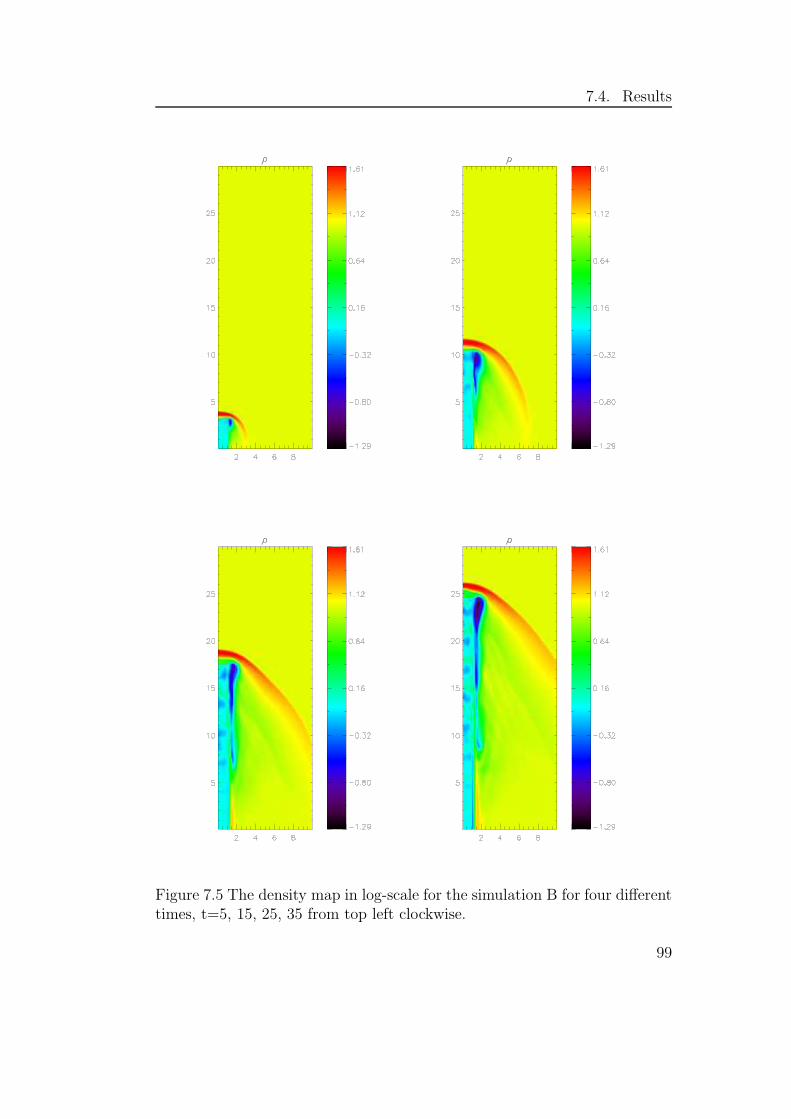
7.4. Results
Figure 7.5 The density map in log-scale for the simulation B for four differenttimes, t=5, 15, 25, 35 from top left clockwise.
99

Chapter 7. MHD Jets
Table 7.2 The quantities below are calculated for the simulation of jets withsteady (simulation A) and variable injection (simulation B). In case of B, themaximum numbers of M are given.
Simulations
A & Bcs int 0.47cs ext 0.24Mint 2.11Mext 4.22Mint 18.6Mext 41Ma 14.5
Figure 7.6 The variable Lorentz factor over the z-axis for r = 0.45rj for t=35.On the left simulation A and on the right simulation B.
Figure 7.7 The conserved relativistic quantity Γρ over the z-axis for r = 0.45rj
for t=35. On the left simulation A and on the right simulation B.
100

7.4. Results
Figure 7.8 The conserved relativistic quantity ρ over the z-axis for r = 0.45rj
for t=35. On the left simulation A and on the right simulation B.
Figure 7.9 The pressure over the z-axis for r = 0.45rj for t=35. On the leftsimulation A and on the right simulation B.
Figure 7.10 The magnetic component Bz over the z-axis for r = 0.45rj fort=35. On the left simulation A and on the right simulation B.
101

Chapter 7. MHD Jets
Figure 7.11 The magnetic component Bφ over the z-axis for r = 0.45rj fort=35. On the left simulation A and on the right simulation B.
the length of the jet. As expected, the jet with the steady Lorentz factor
manages to propagate further than the one in simulation B, since on average
its injection velocity is higher. Despite the variability in the Gamma factor,
in both simulations the flow is decelerated at the jet head by a strong shock
(Mach disc), which partially thermalizes the jet bulk kinetic energy. Once
shocked by the Mach disc, the jet material forms a backflow along the sides
of the jet, clearly visible in the simulations as the dark blue stripe going down
from the jet head. Despite the variability in Γ, in both simulations the flow
is decelerated at the jet head and the Mach disc is formed, which partially
thermalizes the jet bulk kinetic energy. Once shocked by the Mach disc, the
jet material forms a backflow along the sides of the jet, clearly visibly in the
simulations as the dark blue stripe going down from the jet head. However,
the backflow in simulation B is perturbated, possibly because it is influenced
by the not so smooth jet.
In Fig. 7.6 the Lorentz factor is plotted for t=35 along the jet when
r = 0.45rj. It is clear how the Lorentz factor is changing according to
Eq. 7.20 for simulation B (right panel) and that is decreasing as it moves
deeper inside the ambient medium. Such a decrease is expected since the
jet is decelerated while more material is accumulating at the jet termination
shock, decelerating the jet. On the right panel one can see that the Lorentz
factor for simulation a does not show almost any change and towards the end
102

7.4. Results
of the jet there is even a small increase in its value.
In Fig. 7.7 it is plotted the observed quantity Γρ, in Fig. 7.8 the density,
in Fig. 7.9 the thermal pressure, in Fig. 7.10 the Bz and in Fig. 7.11 the Bφ,
along the jet axis at r = 0.45rj and for t = 35. As expected in both cases
at the termination shock there is a strong change in the density and in the
pressure. The change in the density is comparable in both the simulations.
However, simulation A shows higher change in the pressure, from 0.5 to 18,
when in simulation B the maximum pressure is ∼ 10, almost two times lower.
The difference could be because in simulation A the jet has higher velocity
than in simulation B, creating a stronger shock. The result is in accordance
with the estimated Mach numbers. Looking at the plots of the magnetic field
we see that there is no important compression of Bφ as we would like to have
and the change in Bφ is slightly higher in simulation A. However, the value
of Bφ in simulation B is changing periodically as Γ.
7.4.2 Variable Lorentz factor and Differences in Pres-
sure
In this section we present the preliminary results of two simulations, simu-
lation A’ and B. In both of them the Lorentz factor is changing with time
as:
Γ(t) = Max[Γmin, Γmax sin4(t)] (7.21)
with Γmin = 5 and Γmax = 10 (see Fig. 7.3 for a plot of the function).
The parameters chosen for the physical quantities are shown in Table 7.1.
Simulation B is the same as simulation B in Section 7.4.1. The difference
between A’ and B lays on the pressure of the ambient medium. For simulation
A’ Pe = 5 or Pe = 7 × 10⁻¹⁰ Ba and for simulation B Pe = 0.5 or Pe =
7 × 10⁻¹¹ Ba, the same value as the pressure of the jet initially.
The only difference between the two simulations is the value of the pres-
sure inside and out of the jet. However, we can express this difference in the
103

Chapter 7. MHD Jets
Table 7.3 The quantities below are calculated for the simulation A’ and Bfor jets with variable injection profiles.
SimulationsA’ B
cs int 0.56 0.47cs ext 0.24 0.24Mint 1.77 2.11Mext 4.22 4.22Mint 14.6 18.6Mext 41 41Ma 14.5 14.5
value of the plasma β parameter
β =P
B2/2, (7.22)
the ratio between the thermal pressure and the magnetic pressure. This
parameter gives us the relative importance of the thermal pressure over the
magnetic field as the restoring force to any disturbance. If β ≫ 1, then
the magnetic force is negligible on the dynamics but the magnetic field is
still advected by the flow. In the opposite case that β ≪ 1, it is the gas
pressure that is negligible but it can influence slightly the geometry of any
equilibrium. In our case, with the given values of parameters, the initial β
depends on the radial position inside the jet:
β =
101+0.25r2 , simulation A’
11+0.25r2 , simulation B
(7.23)
The maximum value that β can have is 10 or 1 at centre of the jet and
the minimum value is 8 or 0.8 at the jet radius, for simulation A’ and B
respectively. We see that there is a difference of factor of 10 between the
maximum and minimum values of the two simulations, since PA′ = 10PB.
In Fig. 7.4 and 7.12 the density maps of the two simulations are presented
104

7.4. Results
for four different times of the simulation, t=5, 15, 25, 35, so we can see their
evolution in time. We can see in simulation B that the gas is better confined
by the magnetic toroidal field inside the jet. However, in simulation A’
where the thermal pressure is more important compared to the magnetic
force, more complicated morphology is developed in the jet. In addition the
jet in simulation A’ does not propagate as long as in simulation B, z ≃ 24
instead of z ≃ 26. This is expected looking at Fig. 7.13, the Lorentz factor
Γ over z at distance 0.45rj from the centre of the jet. Γ is oscillating over
time but the different layers of the jet with the higher Lorentz factors almost
maintain its value while moving through the jet, left panel of Fig. 7.13. Of
course, it is expected that there will be a deceleration of the jet because
of its interaction with the ambient medium, that is being reflected in the
value of Γ. In A’ case, after z ≃ 10, the jet loses its strict cylindrical shape
and the Lorentz factor of some jet layers that begun with high Γ, have been
decelerated, resulting to a slower jet. But in both cases, it is clear how the
Lorentz factor is changing over time.
We obtain a similar figure if we plot the conserved quantity Γρ that is
observed from Earth, over z, as shown in Fig. 7.14, again for r = 0.45rj
and t=35 (see also the map for t=35 of Γρ in Fig. 7.19). In addition we
can see the final shock created where the jet is moving through the ambient
medium. In case B there is one final shock where the density is changing
from 1 to ∼ 50. In case A’ the density at the final shock has increased from
1 to ∼ 25, but another region with increased density has been formed at
z ≃ 10 with density ∼ 10, see Fig. 7.15. We are interested in having strong
shocks in order to have the right environment for radiation emission. That is
the reason why we should investigate also the behaviour of Bφ, Fig. 7.18, of
pressure, Fig. 7.16. In case B the Bφ is not changing a lot and no important
compression of the magnetic field is present, not even at the final shock.
On the other hand, in case A’ there a two regions where the magnetic field
component is compressed, at the end of the jet and at z = 10. The pressure
shows similar behaviour with the difference that in case B the pressure in
105

Chapter 7. MHD Jets
Figure 7.12 The density map in log scale for the simulation B for four differenttimes, t=5, 15, 25, 35 from top left clockwise.
106

7.4. Results
Figure 7.13 The variable Lorentz factor over the z-axis for r = 0.45j for t=35.On the left simulation A and on the right simulation B.
the final shock is increased more than in case A’. Further investigation is
needed to understand why the magnetic field compression is present only in
simulation A’ and what is happening in z = 10. To be complete, in Fig. 7.17
the z-component of the magnetic field is plotted.
The values of the Mach numbers are on Table 7.3. Both outflows are
supersonic. The Alfven Mach number is Ma = 14.5 for both simulations.
This suggests that the magnetic field does not play a dominant role in the
dynamics of the jets, but it follows the flow. Therefore, in both cases shocks
and plasma compressions will be able to compress and amplify the magnetic
field as well. On the other hand, comparing the two different plasma beta
parameters, we can expect that the jet in simulation B will be more tightly
constrained by the presence of the magnetic field. Although the internal
Mach number of simulation B is a bit higher than the one of simulation A’,
it is actually during simulation A’ that we notice morphology that could be
internal shocks. More investigation on the topic is required.
In summary, our simulations suggest that the behaviour of relativistic pul-
sating jets is strongly influenced by the value of the beta parameter. More-
over, simulations indicate that a bigger value of the plasma beta is more
favorable for the production of the conditions necessary for a strong syn-
chrotron emission. Indeed, the initially less important magnetic field allows
the formation of shocks and structures which lead to higher compression.
107
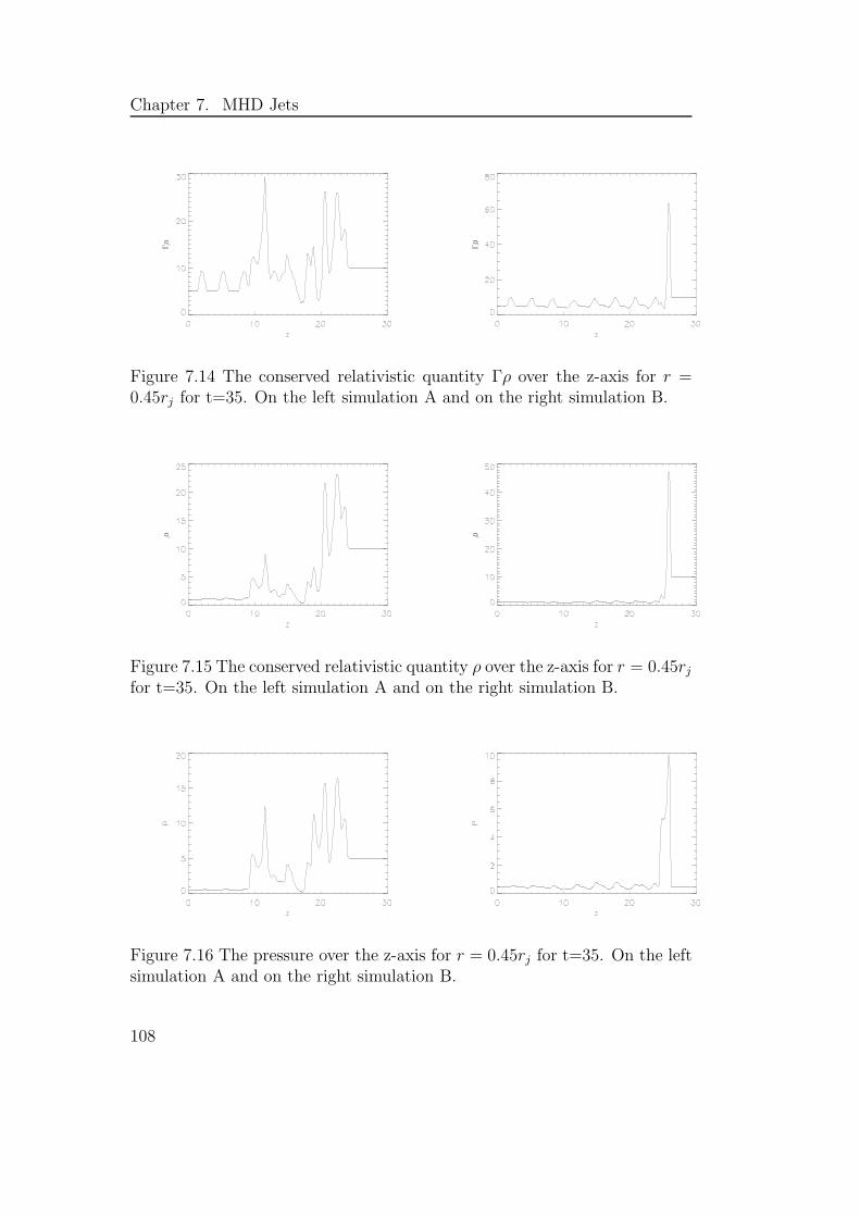
Chapter 7. MHD Jets
Figure 7.14 The conserved relativistic quantity Γρ over the z-axis for r =0.45rj for t=35. On the left simulation A and on the right simulation B.
Figure 7.15 The conserved relativistic quantity ρ over the z-axis for r = 0.45rj
for t=35. On the left simulation A and on the right simulation B.
Figure 7.16 The pressure over the z-axis for r = 0.45rj for t=35. On the leftsimulation A and on the right simulation B.
108

7.4. Results
Figure 7.17 The magnetic component Bz over the z-axis for r = 0.45rj fort=35. On the left simulation A and on the right simulation B.
Figure 7.18 The magnetic component Bφ over the z-axis for r = 0.45rj fort=35. On the left simulation A and on the right simulation B.
Figure 7.19 The variable Lorentz factor over the z-axis for r = 0.45rj fort=35. On the left simulation A and on the right simulation B.
109

Chapter 7. MHD Jets
Further investigation is needed to understand precisely why the magnetic
field compression is present mainly in simulation A’ but almost absent in B,
and what are the dynamical processes leading to the features observed at
z ∼ 10.
110

Conclusions
Nothing exists except atoms and empty space;
everything else is opinion.
-Democritus
The motivation of this dissertation was to better understand the un-
usually hard spectra observed in some blazars, in some cases as hard as
dN/dE ∝ E−1.5, having the observations as a starting point. From what we
observe until the fitting of the spectrum, there is an intermediate challenging
step, the EBL correction. High energy γ-rays are attenuated by the EBL
photon field and the larger the distance to the source, the stronger the ef-
fects are. The spectrum needs to be corrected for this attenuation. The real
challenge lays on the estimation of the EBL spectrum. Observations of EBL
cannot restrict its spectrum sufficiently, some of the problems are the strong
foregrounds difficult to be reduced from the observations or the uncertainties
in the star formation rate and the evolution models applied to estimate the
cosmic EBL evolution. The result is a variety of EBL estimations/models
that influence the final behaviour of the blazars’ intrinsic spectrum since the
attenuation is quite sensitive to the EBL energy density. Trying to cover
different cases, we chose to use two different EBL levels. The first one comes
from the EBL model of Franceschini et al. (2008) (F1.0) and the second one
comes from the scaling of F1.0 by a factor of 1.6 to include a lower limit of
111

Conclusions
EBL derived at 3.6 µm of 9.0+1.7−0.9 nWm−2sr−1 in Levenson & Wright (2008).
It is shown in Chap. 4 that even this small difference of 1.6 can result to a
much harder spectrum, e.g. from dN/dE ∝ E−1.4 to dN/dE ∝ E−0.4 in the
case of 3C 66A, that current models fail to describe.
After the reconstruction of the blazar spectrum, we move directly to
the modeling (Chap. 5) using a proton synchrotron model. Protons are
accelerated in very high energies and produce γ-rays through synchrotron
radiation in the presence of strong magnetic fields. We assume that the
γ-rays are produced inside a blob that moves relativistically with Lorentz
factor Γ. If the blob is moving inside a soft photon field, then we have
internal absorption and the γ-rays will be attenuated due to pair production.
For a Planckian distribution of the soft photons, we show that an arbitrary
hard spectrum can be produced by changing the optical depth of the γ-rays’
attenuation. We show that the sources’ spectrum is fitted by the model,
combining the right values of the magnetic field and the temperature of the
diluted Planckian distribution, for both of the two different EBL spectra.
In addition, the energy lost because of the absorption is transferred to
electron-positron pairs that emit synchrotron radiation in the Optical/X-ray
regime through synchrotron radiation. The secondary pairs that are created
inside the blob have their radiation boosted and possibly detectable, but the
radiation of the pairs created out of the blob cannot be observed because it is
not boosted. The detectable radiation is constrained by the optical depth of
the blob. Although the γ-rays produced by the protons undergo attenuation
as long as they move inside the photon field region, only the part of them that
is absorbed inside the blob will create pairs that in their turn will produce
detectable radiation in the Optical/X-ray regime. The model can describe
the multiwavelength spectrum of 1ES 0229+200 and 3C 66A with success,
taking into account also the upper limits introduced by FERMI LAT in the
GeV regime (Chap. 6).
Towards an attempt to study further the radiation from blazars, we per-
form some numerical simulations (Chap. 7). Knowing that compression of
112

Conclusions
the magnetic field means acceleration of particles and radiation, we search
for a physical configuration that can produce internal shocks, regions promi-
nent to produce synchrotron radiation. Using the numerical code PLUTO
and choosing a basic setup for a relativistic MHD jet with time independent
or time variable Lorentz factor, we investigate the properties of the formed
jet. We are not interested in the launching of the jet but only on the propa-
gation. For a certain configuration, while the Lorentz factor is changing with
time as Γ(t) = Max[Γmin, Γmax sin4(t)], compression of the magnetic field is
produced. The results we presented here are only preliminary and the esti-
mation of radiation was not done. However, our findings are encouraging to
continue the study and find the proper setup that results to internal shocks
and estimate the produced radiation.
A step forward for the current work would be the improvement of the
instrumentation. So far the available Cherenkov telescopes have their max-
imum sensitivity at ∼ TeV and the low energy threshold is at 100 GeV
(except from MAGIC). Distant sources often are detected only when there
is a flare incidence. An increase to the sensitivity of the instruments and a
lower energy threshold would be helpful in order to get high energy spectrum
in a wider energy range and possibly in less observational time. Cherenkov
Telescope Array (CTA) is a promising new project that with its completion
we will have an instrument at least 10 times more sensitive in the region of
0.1−50 TeV and it will allow thousand new sources to be detected (Wagner
et al., 2009). At the same time, the increased sensitivity will allow shorter
observation times, higher time resolution of variable sources (sub-minute res-
olution instead of the current resolution of minutes) and more follow-up ob-
servations.
With the new window on the high energy universe that will open on ob-
servations, we will be able to get detailed spectra from the VHE sources and
if we take advantage of multiwavelength campaigns, we could have simulta-
neous observations in all the energy bands. A more thorough study would
be possible. In addition, more sources will be detected and their spectra will
113

Conclusions
be available for study. It would be interesting to have a larger sample of
blazars to see how many of them have hard spectrum, what are the values of
the physical parameters that our model gives in order to describe them and
whether there is a pattern behind the required parameters.
114

Acronyms
AGN Active Galactic Nuclei . . . . . . . . . . . . . . . . . . . . . . . . . . . . . . . . . . . . . . . . . .11
BE backward evolution . . . . . . . . . . . . . . . . . . . . . . . . . . . . . . . . . . . . . . . . . . . . . 53
BLR Broad Line Regions . . . . . . . . . . . . . . . . . . . . . . . . . . . . . . . . . . . . . . . . . . . . 18
BLRG broad line radio galaxies . . . . . . . . . . . . . . . . . . . . . . . . . . . . . . . . . . . . . . . . 19
CCE cosmic chemical evolution . . . . . . . . . . . . . . . . . . . . . . . . . . . . . . . . . . . . . . 53
CMB Cosmic Microwave Background . . . . . . . . . . . . . . . . . . . . . . . . . . . . . . . . . 50
CTA Cherenkov Telescope Array. . . . . . . . . . . . . . . . . . . . . . . . . . . . . . . . . . . .113
EAS extensive air shower . . . . . . . . . . . . . . . . . . . . . . . . . . . . . . . . . . . . . . . . . . . . 45
EBL Extragalactic Background Light . . . . . . . . . . . . . . . . . . . . . . . . . . . . . . . . 11
FE forward evolution. . . . . . . . . . . . . . . . . . . . . . . . . . . . . . . . . . . . . . . . . . . . . . .53
FSRQ flat spectrum radio Quasars . . . . . . . . . . . . . . . . . . . . . . . . . . . . . . . . . . . . 19
HBL High-energy peaked Blazars . . . . . . . . . . . . . . . . . . . . . . . . . . . . . . . . . . . . 22
HD hydrodynamics . . . . . . . . . . . . . . . . . . . . . . . . . . . . . . . . . . . . . . . . . . . . . . . . . 90
IDV IntraDay Variability . . . . . . . . . . . . . . . . . . . . . . . . . . . . . . . . . . . . . . . . . . . . 24
LBL Low-energy peaked Blazars . . . . . . . . . . . . . . . . . . . . . . . . . . . . . . . . . . . . . 22
MHD Magnetohydrodynamic . . . . . . . . . . . . . . . . . . . . . . . . . . . . . . . . . . . . . . . . . . v
NE no evolution . . . . . . . . . . . . . . . . . . . . . . . . . . . . . . . . . . . . . . . . . . . . . . . . . . . . 53
NLR Narrow Line Regions . . . . . . . . . . . . . . . . . . . . . . . . . . . . . . . . . . . . . . . . . . . 18
NLRG narrow line radio galaxies . . . . . . . . . . . . . . . . . . . . . . . . . . . . . . . . . . . . . . 19
115

Acronyms
OVV optically violent variable. . . . . . . . . . . . . . . . . . . . . . . . . . . . . . . . . . . . . . . .23
QSO Quasi Stellar Objects . . . . . . . . . . . . . . . . . . . . . . . . . . . . . . . . . . . . . . . . . . . 19
RMHD relativistic magnetohydrodynamics . . . . . . . . . . . . . . . . . . . . . . . . . . . . . 90
SA semianalytical . . . . . . . . . . . . . . . . . . . . . . . . . . . . . . . . . . . . . . . . . . . . . . . . . . 53
SED Spectral Energy Distribution . . . . . . . . . . . . . . . . . . . . . . . . . . . . . . . . . . . 22
SSRQ steep spectrum radio Quasars . . . . . . . . . . . . . . . . . . . . . . . . . . . . . . . . . . 19
VHE Very High Energy . . . . . . . . . . . . . . . . . . . . . . . . . . . . . . . . . . . . . . . . . . . . . . . v
116

Aknowledgements
Real life isn’t always going to be perfect or go our way,
but the recurring acknowledgement of what is working in our lives
can help us not only to survive but surmount our difficulties.
-Sarah Ban Breathnach
I feel very privileged that I have so many people to thank. First of all
I would like to thank Prof. Aharonian for his supervision, his inspiration
and passion. I learnt a lot from him and I admire his approach on physics.
Then I would like to thank PD Dr. Fendt for his guidance during my first
contact with numerical simulations and for offering the warmest welcome in
Heidelberg. You are the best IMPRS coordinator we could have asked, with
a lot of patience and will to help. Felix and Christian, thank you for the
opportunity you offered me to work with you and for being the referees of
this thesis. I would like also to thank Prof. Grebel and Prof. Hofmann for
accepting to be part of my examination committee.
My special thanks to Mitya for the scientific collaboration, for reading
my posters/ talks/ proceedings, for installing/ re-installing/ uninstalling so
many programs on my computer and answering all of my questions! Martin,
thank you for helping me with the EBL. Then there is aso Stefano, Sabrina,
Anna, Andrew, Ervin and Emma for all the scientific, technical and personal
discussions! I should also mention the people of ”our corridor” for all the
117

Aknowledgements
nice company during lunches and tea breaks. Many thanks also to Frank for
the German abstract, and Dave and Roland for their corrections in English
(wherever there are mistakes, it is my fault!).
Then there are the people that filled my life outside work and created
beautiful memories to take with me and made sunnier the life of a Mediter-
ranean girl in cold Heidelberg. Starting for the most important person for
me in these years, Matteo. For having this huge amount of patience with
me, for being innocent and full of trust on people, his help with PLUTO,
his comments on my thesis and a lot more things that can be summarized in
”for just being next to me”. Thanks to my unique friends, Giovanna, Sara,
Viviana, Isabel, Denija, Kelly, Giovanni, Lisa, Emma, Massimo. And also,
Giulia, Claudia, Jamie, Baybars, Dusan. There is also Swetlana and Federica
that unfortunately I did not have as much time as I wanted to know them
better but they are very special to me. A special place has also Bambi and
all the girls in her school that the last 2.5 years made me feel comfortable
with them although I could not understand almost anything of what they
were saying in German (!) and made every Thursday an exciting day! Of
course I could not forget to mention my dear ladies, Kelly (again), Kathrin,
Sirin, Anna, Cecile, Claudine and Mr. Dave for all the delicious nights of
our “cooking club”!
Changing country, I would like to thank my family for having faith on me
and my choices. Then there are all of my friends, Anna, Maria, Chryssavghi,
Stamatis, Grigoris, Stavros, Giannis, Giorgos and especially Vassilis for all
the kind of support they offered me during my stay in Heidelberg.
Last but not least, I would like to specially thank Apostolos Mastichiadis
for all the discussions and advice and because without him I wouldn’t have
been in Heidelberg for a Ph.D!
118

References
Abdo, A. A., Ackermann, M., Ajello, M., et al. 2009, Astrphysical Journal,
707, 1310
Acciari, V. A., Aliu, E., Arlen, T., et al. 2009, Astrophysical Journal Letters,
693, L104
Aharonian, F., Akhperjanian, A. G., Barres de Almeida, U., et al. 2007,
Astronomy and Astrophysics, 475, L9
Aharonian, F., Akhperjanian, A. G., Bazer-Bachi, A. R., et al. 2006, Nature,
440, 1018
Aharonian, F. A. 2000, New Astronomy, 5, 377
Aharonian, F. A. 2004, Very high energy cosmic gamma radiation : a crucial
window on the extreme Universe, ed. Aharonian, F. A.
Aharonian, F. A., Atoian, A. M., & Nagapetian, A. M. 1983, Astrofizika, 19,
323
Aharonian, F. A., Khangulyan, D., & Costamante, L. 2008, Monthly Notices
of the Royal Astronomical Society, 387, 1206
Aliu, E., Anderhub, H., Antonelli, L. A., et al. 2009, Astrophysical Journal
Letters, 692, L29
Bai, J. M., Liu, H. T., & Ma, L. 2009, Astrphysical Journal, 699, 2002
119

References
Begelman, M. C., Fabian, A. C., & Rees, M. J. 2008, Monthly Notices of the
Royal Astronomical Society, 384, L19
Bernstein, R. A., Freedman, W. L., & Madore, B. F. 2002, Astrphysical
Journal, 571, 107
Bernstein, R. A., Freedman, W. L., & Madore, B. F. 2005, Astrphysical
Journal, 632, 713
Blandford, R. D. & Payne, D. G. 1982, Monthly Notices of the Royal Astro-
nomical Society, 199, 883
Blumenthal, G. R. & Gould, R. J. 1970, Reviews of Modern Physics, 42, 237
Boettcher, M. & Schlickeiser, R. 1997, Astronomy and Astrophysics, 325,
866
Bonometto, S. & Rees, M. J. 1971, Monthly Notices of the Royal Astronom-
ical Society, 152, 21
Bottcher, M. 2007, Astrophysics and Space Science, 309, 95
Bregman, J. N. 1990, Astronomy and Astrophysics Review, 2, 125
Brown, T. M., Kimble, R. A., Ferguson, H. C., et al. 2000, Astronomical
Journal, 120, 1153
Cambresy, L., Reach, W. T., Beichman, C. A., & Jarrett, T. H. 2001, Astr-
physical Journal, 555, 563
Cole, S., Lacey, C. G., Baugh, C. M., & Frenk, C. S. 2000, Monthly Notices
of the Royal Astronomical Society, 319, 168
Costamante, L., Aharonian, F., Buehler, R., et al. 2009, ArXiv e-prints
Costamante, L., Ghisellini, G., Celotti, A., & Wolter, A. 2002, in Blazar
Astrophysics with BeppoSAX and Other Observatories, ed. P. Giommi,
E. Massaro, & G. Palumbo, 21–+
120
References
Derishev, E. V., Aharonian, F. A., Kocharovsky, V. V., & Kocharovsky,
V. V. 2003, Physical Review D, 68, 043003
Dole, H., Lagache, G., Puget, J., et al. 2006, Astronomy and Astrophysics,
451, 417
Dominguez, A., Primack, J. R., Rosario, D. J., et al. 2010, ArXiv e-prints
Dube, R. R., Wickes, W. C., & Wilkinson, D. T. 1979, Astrphysical Journal,
232, 333
Dwek, E. & Arendt, R. G. 1998, Astrophysical Journal Letters, 508, L9
Edelstein, J., Bowyer, S., & Lampton, M. 2000, Astrphysical Journal, 539,
187
Elbaz, D., Cesarsky, C. J., Chanial, P., et al. 2002, Astronomy and Astro-
physics, 384, 848
Fall, S. M. 2001, in IAU Symposium, Vol. 204, The Extragalactic In-
frared Background and its Cosmological Implications, ed. M. Harwit &
M. G. Hauser, 401–+
Fazio, G. G., Ashby, M. L. N., Barmby, P., et al. 2004, Astrophysical Journal
Supplement Series, 154, 39
Finkbeiner, D. P., Davis, M., & Schlegel, D. J. 2000, Astrphysical Journal,
544, 81
Franceschini, A., Rodighiero, G., & Vaccari, M. 2008, Astronomy and Astro-
physics, 487, 837
Frayer, D. T., Huynh, M. T., Chary, R., et al. 2006, Astrophysical Journal
Letters, 647, L9
Giovannini, G., Cotton, W. D., Feretti, L., Lara, L., & Venturi, T. 2001,
Astrphysical Journal, 552, 508
121

References
Gorjian, V., Wright, E. L., & Chary, R. R. 2000, Astrphysical Journal, 536,
550
Gould, R. J. & Schreder, G. P. 1967, Physical Review, 155, 1408
Hauser, M. G., Arendt, R. G., Kelsall, T., et al. 1998, Astrphysical Journal,
508, 25
Hauser, M. G. & Dwek, E. 2001a, Annual Review of Astronomy and Astro-
physics, 39, 249
Hauser, M. G. & Dwek, E. 2001b, Annual Review of Astronomy and Astro-
physics, 39, 249
Hinton, J. 2009, New Journal of Physics, 11, 055005
Kashlinsky, A., Mather, J. C., Odenwald, S., & Hauser, M. G. 1996, Astr-
physical Journal, 470, 681
Kashlinsky, A. & Odenwald, S. 2000, Astrphysical Journal, 528, 74
Katarzynski, K., Ghisellini, G., Tavecchio, F., Gracia, J., & Maraschi, L.
2006, Monthly Notices of the Royal Astronomical Society, 368, L52
Kneiske, T. M., Bretz, T., Mannheim, K., & Hartmann, D. H. 2004, Astron-
omy and Astrophysics, 413, 807
Kneiske, T. M. & Dole, H. 2010, Astronomy and Astrophysics, 515, A19+
Krennrich, F., Dwek, E., & Imran, A. 2008, Astrophysical Journal Letters,
689, L93
Lagache, G. & Puget, J. L. 2000, Astronomy and Astrophysics, 355, 17
Leinert, C., Bowyer, S., Haikala, L. K., et al. 1998, Astronomy and Astro-
physics Supplement, 127, 1
Levenson, L. R. & Wright, E. L. 2008, Astrphysical Journal, 683, 585
122

References
Levenson, L. R., Wright, E. L., & Johnson, B. D. 2007, Astrphysical Journal,
666, 34
Lichnerowicz, A. 1967, Relativistic Hydrodynamics and Magnetohydrody-
namics, ed. Lichnerowicz, A.
Liu, H. T. & Bai, J. M. 2006, Astrphysical Journal, 653, 1089
Liu, H. T., Bai, J. M., & Ma, L. 2008, Astrphysical Journal, 688, 148
Longair, M. S. 1992, High energy astrophysics. Vol.1: Particles, photons and
their detection, ed. Longair, M. S.
Lonsdale, C. 1996, in American Institute of Physics Conference Series, Vol.
348, American Institute of Physics Conference Series, ed. E. Dwek, 147–158
Madau, P. & Pozzetti, L. 2000, Monthly Notices of the Royal Astronomical
Society, 312, L9
Martin, C., Hurwitz, M., & Bowyer, S. 1991, Astrphysical Journal, 379, 549
Massaglia, S. 2003, Astrophysics and Space Science, 287, 223
Massaglia, S., Bodo, G., & Ferrari, A. 1996, Astronomy and Astrophysics,
307, 997
Matsumoto, T., Matsuura, S., Murakami, H., et al. 2005, Astrphysical Jour-
nal, 626, 31
Mattila, K. 1990, in IAU Symposium, Vol. 139, The Galactic and Extra-
galactic Background Radiation, ed. S. Bowyer & C. Leinert, 257–268
Mazin, D. & Raue, M. 2007, Astronomy and Astrophysics, 471, 439
McBreen, B. 1979, Astronomy and Astrophysics, 71, L19
Metcalfe, L., Kneib, J., McBreen, B., et al. 2003, Astronomy and Astro-
physics, 407, 791
123
References
Mignone, A., Bodo, G., Massaglia, S., et al. 2007, Astrophysical Journal
Supplement Series, 170, 228
Miller, J. S. 1989, in Lecture Notes in Physics, Berlin Springer Verlag, Vol.
334, BL Lac Objects, ed. L. Maraschi, T. Maccacaro, & M.-H. Ulrich,
395–+
Nikishov, A. I. 1962, Sov. Phys. JETP, 14, 393
Norman, M. L., Winkler, K., Smarr, L., & Smith, M. D. 1982, Astronomy
and Astrophysics, 113, 285
Papovich, C., Dole, H., Egami, E., et al. 2004, Astrophysical Journal Sup-
plement Series, 154, 70
Peacock, J. 2000, Cosmological Physics (Cambridge University Press), 355
Peebles, P. J. E. 1993, Principles of physical cosmology, ed. Peebles, P. J. E.
Prandini, E., Bonnoli, G., Maraschi, L., Mariotti, M., & Tavecchio, F. 2010,
Monthly Notices of the Royal Astronomical Society, 405, L76
Primack, J. R., Gilmore, R. C., & Somerville, R. S. 2008, in American Insti-
tute of Physics Conference Series, Vol. 1085, American Institute of Physics
Conference Series, ed. F. A. Aharonian, W. Hofmann, & F. Rieger, 71–82
Primack, J. R., Somerville, R. S., Bullock, J. S., & Devriendt, J. E. G. 2001,
in American Institute of Physics Conference Series, Vol. 558, American
Institute of Physics Conference Series, ed. F. A. Aharonian & H. J. Volk,
463–478
Reimer, A. 2007, Astrphysical Journal, 665, 1023
Reyes, L. C., for the Fermi LAT collaboration, & the VERITAS collaboration.
2009, ArXiv e-prints
Rybicki, G. B. & Lightman, A. P. 1986, Radiative Processes in Astrophysics,
ed. Rybicki, G. B. & Lightman, A. P.
124

References
Scheck, L., Aloy, M. A., Martı, J. M., Gomez, J. L., & Muller, E. 2002,
Monthly Notices of the Royal Astronomical Society, 331, 615
Sitarek, J. & Bednarek, W. 2008, Monthly Notices of the Royal Astronomical
Society, 391, 624
Tavecchio, F. & Ghisellini, G. 2008, Monthly Notices of the Royal Astronom-
ical Society, 386, 945
Tavecchio, F., Ghisellini, G., Ghirlanda, G., Costamante, L., & Franceschini,
A. 2009, Monthly Notices of the Royal Astronomical Society, 399, L59
Tavecchio, F. & Mazin, D. 2009, Monthly Notices of the Royal Astronomical
Society, 392, L40
Toller, G. N. 1983, Astrophysical Journal Letters, 266, L79
Urry, C. M. & Padovani, P. 1995, Publications of the Astronomical Society
of the Pacific, 107, 803
Wagner, R. M., Lindfors, E. J., Sillanpaa, A., et al. 2009, ArXiv e-prints
Wright, E. L. & Reese, E. D. 2000, Astrphysical Journal, 545, 43
Zirakashvili, V. N. & Aharonian, F. 2007, Astronomy and Astrophysics, 465,
695
125