Embed Size (px)
Citation preview
Eotvos Lorand University of Siences
Multi-scale modeling of Li-ion batteries
BSc Thesis
Prepared by
Laszlo Zeno Farkas
Bachelor Sciences (BSc) in Mathematics
Department of Applied Analysis and
Computational Mathematics
Supervisors:Akos Kriston
European Commission, DG Joint Research Centre,
Institute for Energy and Transport
Istvan Farago
Eotvos Lorand University Faculty of Science
Department of Applied Analysis and
Computational Mathematics
2015Budapest

Declaration of Authorship
Nev: Farkas Laszlo Zeno
ELTE Termeszettudomanyi Kar, szak: Elemzo matematikus
NEPTUN azonosıto: RRRKWJ
Szakdolgozat cıme: Multi-scale modeling of Li-ion batteries
A szakdolgozat szerzojekent fegyelmi felelossegem tudataban kijelentem, hogy a dol-
gozatom onallo munkam eredmenye, sajat szellemi termekem, abban a hivatkozasok
es idezesek standard szabalyait kovetkezetesen alkalmaztam, masok altal ırt reszeket a
megfelelo idezes nelkul nem hasznaltam fel.
Budapest, 2015
hallgato alaırasa
iii
Acknowledgements
I would like to thank Akos Kriston research fellow of JRC Institute for Energy and
Transport Petten, that I could work with him on this topic, in Hungary and abroad
during my traineeship. I would like to thank the many consultations which significantly
contributed to the deeper understanding of Lithium-ion batteries, as well the support
which gave me strength to progression of thesis and work.
I would like to thank Dr. Istvan Farago, professor of Eotvos Lorand University and head
of Department of Applied Analysis and Computational Mathematics, for consultations,
inspirations and advices.
The continuous support of Dr. Lois Brett, the project leader of Battery Energy Storage
Testing for Safe Electrification of Transport (BESTEST), is highly appreciated. The
fruitful discussion of Dr. Andreas Pfrang about the thesis and his advices are acknowl-
edged.
I would like to thank also all of my colleagues at JRC Institute for Energy and Transport
for their contribution, useful instructions to my professional development and daily work.
iv
Contents
Declaration of Authorship iii
Acknowledgements iv
1 Introduction 1
1.1 Partial differential equations . . . . . . . . . . . . . . . . . . . . . . . . . . 5
1.2 Sequential splitting . . . . . . . . . . . . . . . . . . . . . . . . . . . . . . . 7
1.3 Governing equations of a typical Li-ion battery model . . . . . . . . . . . 9
2 Development of mathematical model of a lithium-ion batteriy 13
2.1 Derivation of the general partial differential equation system . . . . . . . . 13
2.2 Derivation of the canonical form of equations . . . . . . . . . . . . . . . . 15
2.2.1 Electric potential in the solid phase (ϕ1) and electric potential inthe electrolyte phase (ϕ2) . . . . . . . . . . . . . . . . . . . . . . . 15
2.2.2 Concentration of Li+ ions in the electrolyte phase . . . . . . . . . 22
2.2.3 Concentration of Li+ ions in the solid particle . . . . . . . . . . . 23
2.3 Solution in Matlab by using ”pdepe” solver . . . . . . . . . . . . . . . . . 24
2.4 Modifications of the partial differential equation system . . . . . . . . . . 28
2.4.1 Introduction of reference potential . . . . . . . . . . . . . . . . . . 28
2.4.2 Introduction of time dependent boundary conditions . . . . . . . . 31
3 Solution of the model and the results 35
3.1 Solution of the partial differential equation system by operator splitting . 35
3.1.1 Analytical solution of the splitted problems . . . . . . . . . . . . . 36
3.1.2 Numerical solution of the splitted problems . . . . . . . . . . . . . 40
3.1.3 Comparison of exact and splitting solutions . . . . . . . . . . . . . 48
3.2 Accuracy of the splitting solution . . . . . . . . . . . . . . . . . . . . . . . 50
4 Conclusions and outlook 57
A Symbols in the equations 59
B Parameters in the program codes 61
C Matlab codes 63
C.1 Solution of Matlab ”pdepe” solver in Section 2.3 . . . . . . . . . . . . . . 63
v

Contents vi
C.2 Numerical solution in Subsection 3.1.2 . . . . . . . . . . . . . . . . . . . . 64
C.3 Explicit-Euler’s method in Subsection 3.2 . . . . . . . . . . . . . . . . . . 66
Bibliography 69
Chapter 1
Introduction
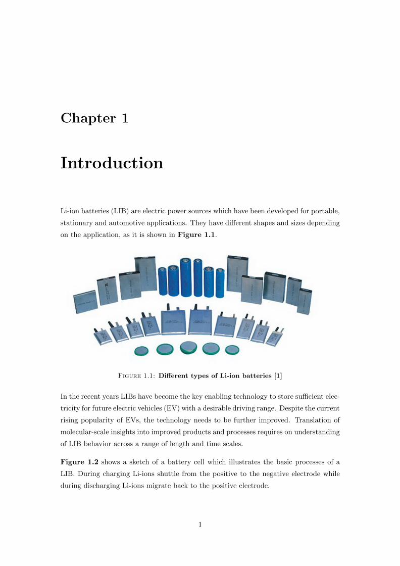
Li-ion batteries (LIB) are electric power sources which have been developed for portable,
stationary and automotive applications. They have different shapes and sizes depending
on the application, as it is shown in Figure 1.1.
Figure 1.1: Different types of Li-ion batteries [1]
In the recent years LIBs have become the key enabling technology to store sufficient elec-
tricity for future electric vehicles (EV) with a desirable driving range. Despite the current
rising popularity of EVs, the technology needs to be further improved. Translation of
molecular-scale insights into improved products and processes requires on understanding
of LIB behavior across a range of length and time scales.
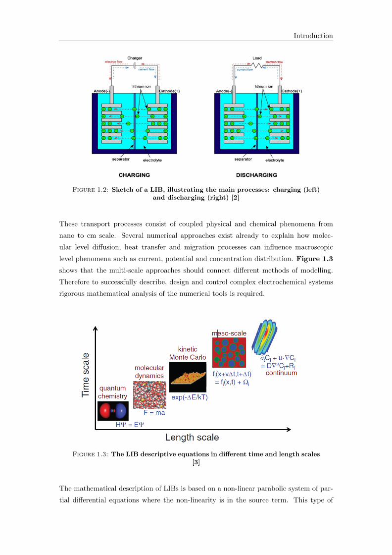
Figure 1.2 shows a sketch of a battery cell which illustrates the basic processes of a
LIB. During charging Li-ions shuttle from the positive to the negative electrode while
during discharging Li-ions migrate back to the positive electrode.
1
Introduction
Figure 1.2: Sketch of a LIB, illustrating the main processes: charging (left)and discharging (right) [2]
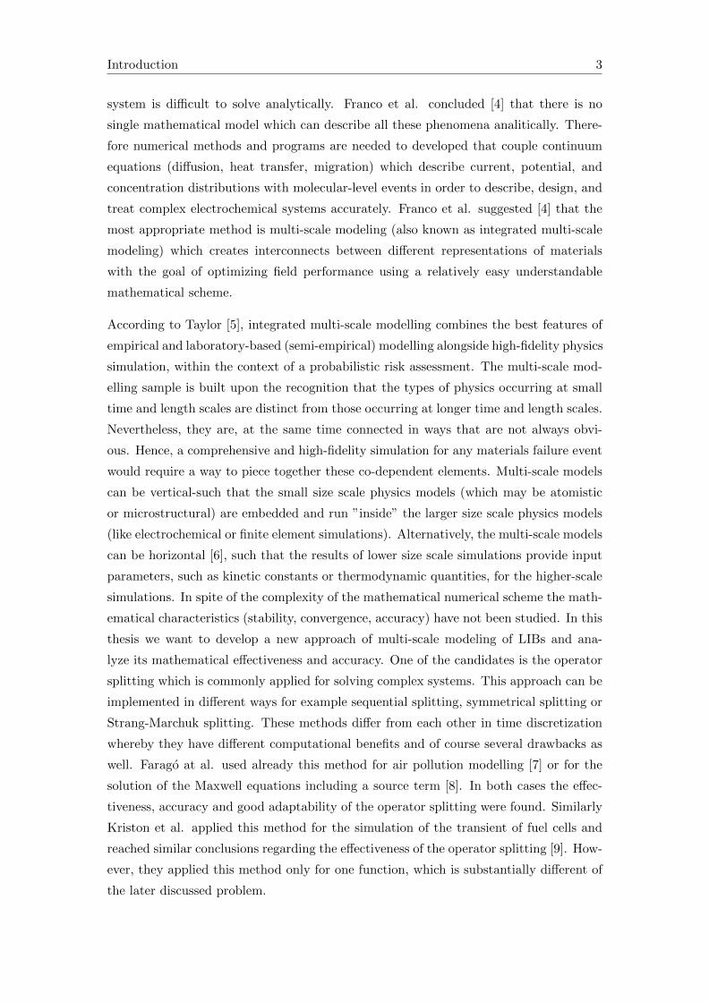
These transport processes consist of coupled physical and chemical phenomena from
nano to cm scale. Several numerical approaches exist already to explain how molec-
ular level diffusion, heat transfer and migration processes can influence macroscopic
level phenomena such as current, potential and concentration distribution. Figure 1.3
shows that the multi-scale approaches should connect different methods of modelling.
Therefore to successfully describe, design and control complex electrochemical systems
rigorous mathematical analysis of the numerical tools is required.
Figure 1.3: The LIB descriptive equations in different time and length scales[3]
The mathematical description of LIBs is based on a non-linear parabolic system of par-
tial differential equations where the non-linearity is in the source term. This type of
Introduction 3
system is difficult to solve analytically. Franco et al. concluded [4] that there is no
single mathematical model which can describe all these phenomena analitically. There-
fore numerical methods and programs are needed to developed that couple continuum
equations (diffusion, heat transfer, migration) which describe current, potential, and
concentration distributions with molecular-level events in order to describe, design, and
treat complex electrochemical systems accurately. Franco et al. suggested [4] that the
most appropriate method is multi-scale modeling (also known as integrated multi-scale
modeling) which creates interconnects between different representations of materials
with the goal of optimizing field performance using a relatively easy understandable
mathematical scheme.
According to Taylor [5], integrated multi-scale modelling combines the best features of
empirical and laboratory-based (semi-empirical) modelling alongside high-fidelity physics
simulation, within the context of a probabilistic risk assessment. The multi-scale mod-
elling sample is built upon the recognition that the types of physics occurring at small
time and length scales are distinct from those occurring at longer time and length scales.
Nevertheless, they are, at the same time connected in ways that are not always obvi-
ous. Hence, a comprehensive and high-fidelity simulation for any materials failure event
would require a way to piece together these co-dependent elements. Multi-scale models
can be vertical-such that the small size scale physics models (which may be atomistic
or microstructural) are embedded and run ”inside” the larger size scale physics models
(like electrochemical or finite element simulations). Alternatively, the multi-scale models
can be horizontal [6], such that the results of lower size scale simulations provide input
parameters, such as kinetic constants or thermodynamic quantities, for the higher-scale
simulations. In spite of the complexity of the mathematical numerical scheme the math-
ematical characteristics (stability, convergence, accuracy) have not been studied. In this
thesis we want to develop a new approach of multi-scale modeling of LIBs and ana-
lyze its mathematical effectiveness and accuracy. One of the candidates is the operator
splitting which is commonly applied for solving complex systems. This approach can be
implemented in different ways for example sequential splitting, symmetrical splitting or
Strang-Marchuk splitting. These methods differ from each other in time discretization
whereby they have different computational benefits and of course several drawbacks as
well. Farago at al. used already this method for air pollution modelling [7] or for the
solution of the Maxwell equations including a source term [8]. In both cases the effec-
tiveness, accuracy and good adaptability of the operator splitting were found. Similarly
Kriston et al. applied this method for the simulation of the transient of fuel cells and
reached similar conclusions regarding the effectiveness of the operator splitting [9]. How-
ever, they applied this method only for one function, which is substantially different of
the later discussed problem.
4 Introduction
The most common LIB model developed by Newman et al. [10] uses different numerical
schemes, such as explicit, implicit or IMEX method, which are different in terms of
solution procedure:
Explicit: The solution for (n+ 1)th step can be written from the solution for nth step.
Implicit: This method finds a solution by solving an algebraic equation involving both
the current ((n+ 1)th) state of the system and the earlier (nth) one.
IMEX: In such a procedure, the advection and diffusion terms are discretized implicitly
in time and the reaction terms explicitly [11].
However, the use of these methods for complex problems is often time-consuming and
inaccurate, and therefore they are not very effective. The main advantage of operator
splitting techniques, in regards of multi-scale modeling, is the availability to use the
different numerical schemes and methods at different length and time scales. The main
drawback may be the loss of stability and accuracy because the splitting error might
bring a new source of inaccuracy. Because operator splitting has not been applied for the
simulation of LIB, in this work an adequate mathematical model is developed and the
aim is to apply an operator splitting scheme and study its applicability as a multi-scale
modelling tool.
The other important objectives are:
a, To study the effectiveness of the splitting method and compare it to other com-
monly applied methods (for example an explicit finite different method).
b, To find a way to use it for multi-scale modeling of complex systems.
Therefore in this work we deal with the following themes: In Section 1.1-1.2 some
basic definition from the theory of partial differential equations (PDEs) and of sequential
splitting are detailed. In Section 1.3 we introduce the LIBs governing basic equations,
parameters and variables which mathematical models are discussed in Chapter 2. The
slightly simplified problem inSection 2.1 are converted in to a solvable form (canonical
form) and discussed in Section 2.2. We solve the PDE-system in Section 2.3 using
Matlab ”pdepe” solver and we analyze the results. In Section 2.4 we modify the PDE-
system in order to reach realistic results and to see their effects on the independent
variables. In Chapter 3 is furthermore the standard method of sequential splitting
introduced and is applied its method to our problem. In Subsections 3.1.1-3.1.2
we solve the PDE-system by using sequential splitting. In the first case we present a
method to find a solution by analytical techniques. Advantages of this method are that
Introduction 5
they are easy to use and sub-processes are simpler which result an easier analysis of
errors. However the disadvantage is that the exact solution can’t be determined for
complex systems such as batteries. In the second case we try to find a solution in
a numerical way where an finite difference method (FDM) is used which calculates a
numerical approximation of the solution and determine the values of the functions at
certain points. In Subsection 3.1.3 we compare the solution of the splitting method
with the solution of the Matlab ”pdepe” solver furthermore the errors and the stability
are analyzed. Furthermore we analyzed stability, convergence and errors of methods
which are described in the Section 3.2. In the last chapter is an outlook provided for
the additional capabilities and applications of a multi-scale modeling. In the thesis used
parameters, program codes and notations can be found in Appendix A, B and C.
Beside the theoretical results, this research is in a closed connection with my trainee
work at The European Commission Joint Research Centre, Institute for Energy and
Transport, where my main task was to test and analyze numerical simulation soft-
ware which can simulate a LIB in 3D and has the possibility to handle the governing
equations on very basic levels i.e. the rewriting the program codes. Several software
products exist on the market which can simulate a LIB (they are used to simulate other
energy storage devices as well). They can be used to simulated battery’s capacity, the
cycling performance, the internal processes and the impact of external factors on the
performance. These software (Fortran, Matlab, COMSOL, Abaqus, ANSYS e.g.) prod-
ucts usually have different source codes and they are based on different mathematical
methods, which have different errors and accuracy, therefore it is worth examining the
consistency, stability and convergence. These software are typically not free, but rather
require quite expensive licenses. That is why it is so important to be sure before the
purchase that they are able to solve the given tasks. Therefore our developed model
system and methods can be used to test the capability of these software tools for multi-
scale modelling.
1.1 Partial differential equations
A partial differential equation (PDE) [12] contains some relation between the unknown
multivariable functions and their partial derivatives. Usually PDEs include time-, and
space-dependent functions of different order. The general form in the Ω ⊂ R2 domains
is
6 Introduction
(Lu)(x, t) = a(x, t)∂2u
∂x2+ 2b(x, t)
∂2u
∂x∂t+ c(x, t)
∂2u
∂t2+
+d(x, t)∂u
∂x+ e(x, t)
∂u
∂t+ g(x, t)u(x, t) = f(x, t)
where a, b, c, d, e, g, are given coefficient functions, f (the so called source function)
defined by the physical model. In this case L is called operator. The following part is
called main part of operator L:
(L0u)(x, t) = a(x, t)∂2u
∂x2+ 2b(x, t)
∂2u
∂x∂t+ c(x, t)
∂2u
∂t2.
Definition 1.1. Operator L is called
elliptic type in the point (x, t) ∈ Ω, if L0 satisfies the following condition:
a(x, t)c(x, t)− b2(x, t) > 0
parabolic type in the point (x, t) ∈ Ω, if L0 satisfies the following condition:
a(x, t)c(x, t)− b2(x, t) = 0
hiperbolic type in the point (x, t) ∈ Ω, if L0 satisfies the following condition:
a(x, t)c(x, t)− b2(x, t) < 0 .
We can define more initial condition at t = 0 and at the boundary of the domain
boundary conditions. The boundary conditions have three types:
• Dirichlet boundary conditions:
u(a, t) = µ1(t), u(b, t) = µ2(t), t > 0
• Neumann boundary conditions:
∂u
∂x(a, t) = µ1(t),
∂u
∂x(b, t) = µ2(t), t > 0
• Robin boundary conditions:
c1u(a, t) +∂u
∂x(a, t) = µ1(t), c1u(b, t) +
∂u
∂x(b, t) = µ2(t), t > 0
Here µ1, µ2 are given functions and c1 ∈ R given number In the following we deal
only with second order PDEs. Some examples, with appropriate initial and boundary
conditions, are the followings:
Introduction 7
1. Laplace-equation:
∂2u
∂x2(x, y) +
∂2u
∂y2(x, y) = 0
2. Poisson equation:
∂2u
∂x2(x, y) +
∂2u
∂y2(x, y) = f(x, y)
3. Heat conduction equation with source term:
∂u
∂t(x, t)− ∂2u
∂x2(x, t) = f(x, t)
4. Wave equation with source term:
∂2u
∂t2(x, t)− ∂2u
∂x2(x, t) = f(x, t)
1.2 Sequential splitting
Splitting methods are generally used [7],[8],[9] to solve partial differential equations or
equation system. The main idea is to lead the complex problem to the sequence of
sub-problems with simpler structure.
In the following the general method of sequential splitting [13] is presented briefly for
the solution of parabolic PDE.
Take the following general parabolic PDE-system on [0, T ] time interval which is de-
scribed by the following PDE canonical form and enabled with some suitable initial and
boundary conditions:
∂w
∂t(x, t) =
∂2w
∂x2(x, t) + f(x, t), x ∈ (0, 1), t > 0
w(x, 0) = w0(x),∂w
∂x(0, t) = g1(t),
∂w
∂t(L, t) = g2(t)
where f is a given function (in our case f means the non-linear source term). Let
τ := TNT
be the splitting time step size, where NT ∈ N and let we solve our problem on
the mesh ωτ = nτ ;n = 1, 2, . . . , NT .
The original problem (or the operator of the problem) is splitted to two sub-problems
defined by the following equations and algorithm. The sequential splitting method solves
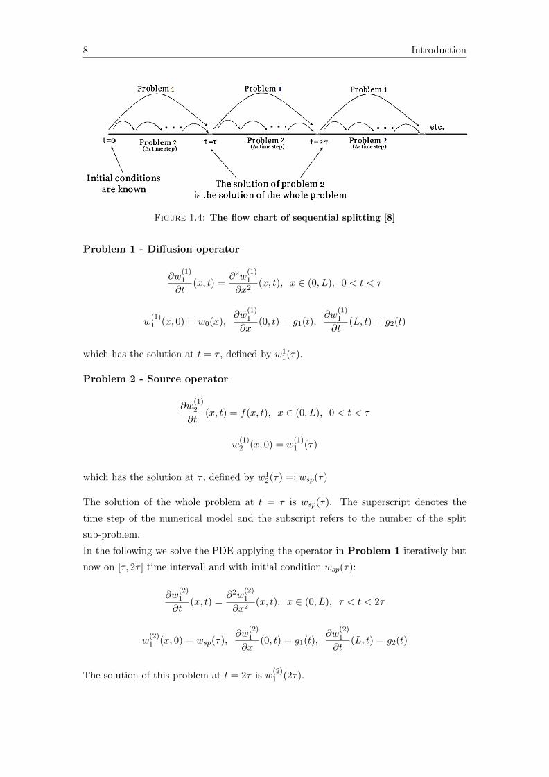
the problem iteratively by applying the steps depicted on Figure 1.4.
8 Introduction
Figure 1.4: The flow chart of sequential splitting [8]
Problem 1 - Diffusion operator
∂w(1)1
∂t(x, t) =
∂2w(1)1
∂x2(x, t), x ∈ (0, L), 0 < t < τ
w(1)1 (x, 0) = w0(x),
∂w(1)1
∂x(0, t) = g1(t),
∂w(1)1
∂t(L, t) = g2(t)
which has the solution at t = τ , defined by w11(τ).
Problem 2 - Source operator
∂w(1)2
∂t(x, t) = f(x, t), x ∈ (0, L), 0 < t < τ
w(1)2 (x, 0) = w
(1)1 (τ)
which has the solution at τ , defined by w12(τ) =: wsp(τ)
The solution of the whole problem at t = τ is wsp(τ). The superscript denotes the
time step of the numerical model and the subscript refers to the number of the split
sub-problem.
In the following we solve the PDE applying the operator in Problem 1 iteratively but
now on [τ, 2τ ] time intervall and with initial condition wsp(τ):
∂w(2)1
∂t(x, t) =
∂2w(2)1
∂x2(x, t), x ∈ (0, L), τ < t < 2τ
w(2)1 (x, 0) = wsp(τ),
∂w(2)1
∂x(0, t) = g1(t),
∂w(2)1
∂t(L, t) = g2(t)
The solution of this problem at t = 2τ is w(2)1 (2τ).
Introduction 9
Now we solve the PDE applying only operator in Problem 2, with appropiate changes
on [τ, 2τ ] time intervall
∂w(2)2
∂t(x, t) = f(x, t), x ∈ (0, L), τ < t < 2τ
w(2)2 (x, τ) = w
(2)1 (x, 2τ)
The solution of this problem at t = 2τ is w(2)2 (2τ) = wsp(2τ).
By solving the previous n steps iteratively, the constructed wsp(nτ) is the solution of
splitting on the given ωh,τ mesh which is defined as follows:
ωh,τ =
(xi, tn); xi = ih; tn = nτ ;h =
L
Nx; τ =
T
NT; i = 1, 2, . . . , Nx; n = 1, 2, . . . , NT
where Nx, NT are the numbers of division parts in space and time.
1.3 Governing equations of a typical Li-ion battery model
In this section the physical model of a LIB is presented. Later a general continuum
mathematical model is defined and simplified, preserving the main characteristics of the
original problem. This simplified PDE-system is discretized by sequential splitting tech-
nique and its accuracy is analyzed in Section 3.2.
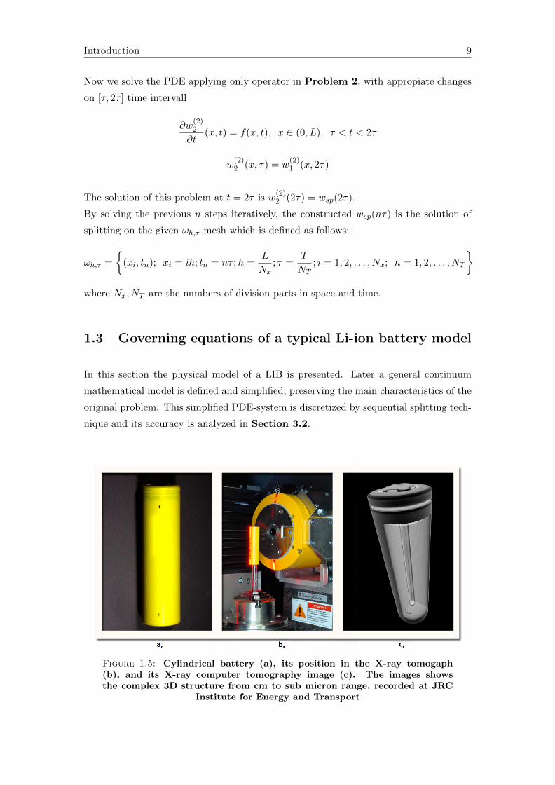
Figure 1.5: Cylindrical battery (a), its position in the X-ray tomogaph(b), and its X-ray computer tomography image (c). The images showsthe complex 3D structure from cm to sub micron range, recorded at JRC
Institute for Energy and Transport
10 Introduction
Figure 1.5.a shows a cylindrical battery, its position in the X-ray tomograph (Figure
1.5.b) and the real X-ray tomography image (Figure 1.5.c). The complex structure
consists of 3 main domains, the cell (Figure 1.6 a) in which the electrode (Figure 1.6
b) is rolled up, and the porous active materials (Figure 1.6 c) where the electrochem-
ical reactions take place.
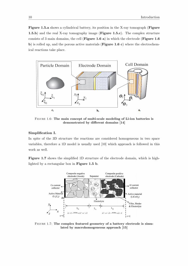
Figure 1.6: The main concept of multi-scale modeling of Li-ion batteries isdemonstrated by different domains [14]
Simplification I.
In spite of the 3D structure the reactions are considered homogeneous in two space
variables, therefore a 1D model is usually used [10] which approach is followed in this
work as well.
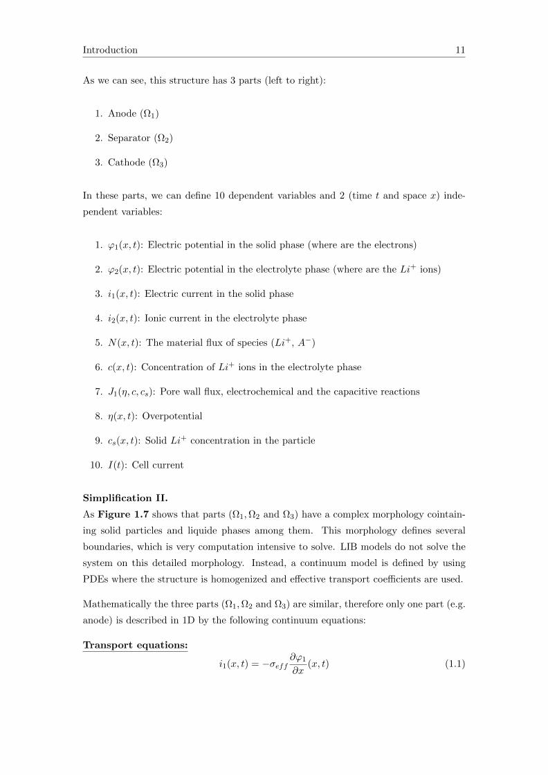
Figure 1.7 shows the simplified 1D structure of the electrode domain, which is high-
lighted by a rectangular box in Figure 1.5 b.
Figure 1.7: The complex featured geometry of a battery electrode is simu-lated by macrohomogeneous approach [15]
Introduction 11
As we can see, this structure has 3 parts (left to right):
1. Anode (Ω1)
2. Separator (Ω2)
3. Cathode (Ω3)
In these parts, we can define 10 dependent variables and 2 (time t and space x) inde-
pendent variables:
1. ϕ1(x, t): Electric potential in the solid phase (where are the electrons)
2. ϕ2(x, t): Electric potential in the electrolyte phase (where are the Li+ ions)
3. i1(x, t): Electric current in the solid phase
4. i2(x, t): Ionic current in the electrolyte phase
5. N(x, t): The material flux of species (Li+, A−)
6. c(x, t): Concentration of Li+ ions in the electrolyte phase
7. J1(η, c, cs): Pore wall flux, electrochemical and the capacitive reactions
8. η(x, t): Overpotential
9. cs(x, t): Solid Li+ concentration in the particle
10. I(t): Cell current
Simplification II.
As Figure 1.7 shows that parts (Ω1,Ω2 and Ω3) have a complex morphology cointain-
ing solid particles and liquide phases among them. This morphology defines several
boundaries, which is very computation intensive to solve. LIB models do not solve the
system on this detailed morphology. Instead, a continuum model is defined by using
PDEs where the structure is homogenized and effective transport coefficients are used.
Mathematically the three parts (Ω1,Ω2 and Ω3) are similar, therefore only one part (e.g.
anode) is described in 1D by the following continuum equations:
Transport equations:
i1(x, t) = −σeff∂ϕ1
∂x(x, t) (1.1)
12 Introduction
i2(x, t) = −κeff∂ϕ2
∂x(x, t)+
+κeffRT
F
[1 +
∂ ln fA(c(x, t))
∂ ln c(x, t)(1− t0+)
∂ ln c(x, t)
∂x(x, t)
](1.2)
N+−(x, t) =∞∑
n=−∞
(νnD
∂c
∂x(x, t) +
i2t0n
znF
)(1.3)
Kinetic equations:
J2(η, c, cs) = an,pi0(cmax − cs(x, t))αn(cs(x, t))αp(c(x, t))αp ·
·[exp
(αnF
RTη(x, t)
)− exp
(−αpFRT
η(x, t)
) ](1.4)
and
J1(η, η2, c, cs) = J2(η, c, cs) + an,pCdl∂η2∂t
(x, t) (1.5)
where
η(x, t) = ϕ1(x, t)− ϕ2(x, t)− ϕref (cs(x, t))−J2(η, c, cs)
an,pRSEI (1.6)
η2(x, t) = ϕ1(x, t)− ϕ2(x, t) (1.7)
(1− εn,p)∂cs∂t
(x, t) = −J2(η, c, cs)F
(1− t0+) (1.8)
Control variable:
I(t) = I = constant (1.9)
The meaning of used symbols in (1.1)-(1.9) can be found in the Appendix A. These
equations describe completely the LIB, however they cannot be solved in this form. In
the next chapter we transform these equations to mathematically solvable (canonical)
form.
Chapter 2
Development of mathematical
model of a lithium-ion batteriy
2.1 Derivation of the general partial differential equation
system
The described problem in (1.1)-(1.9) is not well posed because it has 2 independent
(x, t) and 10 dependent variables, but only 7 governing equations ((1.1)-(1.4), (1.6) and
(1.8)-(1.9)), and several missing boundary conditions.
Remark 2.1. For simplicity the f := f(x, t) notation will be used for the functions.
However, from the electrochemistry we know some relationship between the functions
of this system, for example charge conservation and material balance.
Applying conservation of charge we reach:
∂
∂x(i1 + i2) = 0 . (2.1)
Combining (2.1) with (1.1), (1.2) and the source term (1.5) we reach
− ∂
∂x
(σeff
∂ϕ1
∂x
)+ J1 = 0 (2.2)
and
− κeff∂ϕ2
∂x(x, t) +
κeffRT
F·[
1 +∂ ln fA(c(x, t))
∂ ln c(x, t)(1− t0+)
∂ ln c(x, t)
∂x(x, t)
]− J1 = 0 .
(2.3)
13
Development of mathematical modelling of lithium-ion batteries
If we apply material balance (conservation) to (1.3) and the Gauss-Ostrogradsky-theorem
(divergence theorem), we reach the following equation
∂
∂x
(D∂c
∂x
)− i2z+ν+F
∂t0+∂x
+(1− t0+)
FJ2 = εn,p
∂c
∂t. (2.4)
Simplification III.
If the transference number (t0+) is supposed to be homogeneous (i.e. without variation
in x), than (2.4) can be simplified:
∂
∂x
(D∂c
∂x
)+
(1− t0+)
FJ2 = εn,p
∂c
∂t. (2.5)
So now we have 5 dependent variables (ϕ1, ϕ2, c, cs, J1,2) and 5 governing Eqs.
The physical boundary conditions are:
i1(0, t) = I, i2(0, t) = 0, t > 0 (2.6)
and
i1(L, t) = 0, i2(L, t) = I, t > 0 . (2.7)
Remark 2.2. Boundary conditions (2.6) and (2.7) guarantee, that the electric current
(i1) converted fully to ionic current (i2).
Combining (2.6) with ϕ1 and (2.7) with ϕ2, which boundary conditions of the PDE (2.2)
and (2.3) during electrochemical reaction (J2)
∂ϕ1
∂x=−Iσeff
, −κeff∂ϕ2
∂x+κeffRT
F
(1 +
∂ ln fA(c)
∂ ln c
)(1− t0+)
∂ ln c
∂x= 0, at x = 0
(2.8)
and
∂ϕ1
∂x= 0, −κeff
∂ϕ2
∂x+κeffRT
F
(1 +
∂ ln fA(c)
∂ ln c
)(1−t0+)
∂ ln c
∂x= I, at x = L . (2.9)
Because of there is no material flow from and in the system [10], it implies:
∂c
∂x= 0, at x = 0, L, t > 0 . (2.10)
In the solid particles in the sub-domain can be described the boundary conditions as
well:∂cs∂x
= 0, at x = 0, L, t > 0 . (2.11)
Development of mathematical modelling of lithium-ion batteries 15
The initial conditions can be derived from electrochemistry:
ϕ1(x, 0) = ϕ2(x, 0) = 0, c(x, 0) = c0, cs(x, 0) = csnp, x ∈ [0, L] . (2.12)
and now the equation system (2.2), (2.3), (2.5) and (1.8) are well posed with the bound-
ary conditions (2.8), (2.9), (2.10), (2.11) and with the initial conditions in (2.12).
2.2 Derivation of the canonical form of equations
(2.2), (2.3), (2.5) and (2.11) can be simplifield further by calculating the canonical form
in a dimensionless form. It means that we transform the (2.3), (2.5) and (2.11) to unified
space and time variable and express ϕ1 and ϕ2 with η, which reduces the number of
equations. This is called as the dimensionless canonical form of equations.
2.2.1 Electric potential in the solid phase (ϕ1) and electric potential
in the electrolyte phase (ϕ2)
Substitute J1 in (2.3) and after re-arrangement we reach
− ∂
∂x
(κeff
∂ϕ2
∂x
)+
∂
∂x
[κeffRT
F
(1 +
∂ ln fA(c)
∂ ln c
)(1− t0+)
∂ ln c
∂x
]=
= an,pi0(cmax − cs)αn(cs)αp(c)αp
[exp
(αnF
RTη
)− exp
(−αpFRT
η
) ]+ an,pCdl
∂η2∂t
.
(2.13)
Simplification IV.
1. α = αn = αp = 1
2. (cmax − cs)αn(cs)αp(c)αp = (cmax − cs)(cs)(c)
3. η = η2 = ϕ1 − ϕ2
Consequences:
If we select α = αn = αp = 1, than (2.13) can be rewritten to the following form:
exp
(αnF
RTη
)− exp
(−αpFRT
η
)= 2 sinh
(F
RTη
)(2.14)
and we reach
16 Development of mathematical modelling of lithium-ion batteries
− ∂
∂x
(κeff
∂ϕ2
∂x
)+
∂
∂x
[κeffRT
F
(1 +
∂ ln fA(c)
∂ ln c
)(1− t0+)
∂ ln c
∂x
]=
= an,pi0(cmax − cs)αn(cs)αp(c)αp2 sinh
(F
RTη
)+ an,pCdl
∂η
∂t. (2.15)
Our next goal is to express ϕ2 from (2.15) by function of η. Let η? be
η?(x, t) =F
RTη(x, t) (2.16)
and consequently:∂η?
∂t(x, t) =
F
RT
∂η
∂t(x, t) (2.17)
By substituting (2.16) and (2.17) into (2.15) we reach:
− ∂
∂x
(κeff
∂ϕ2
∂x
)+
∂
∂x
[κeffRT
F
(1 +
∂ ln fA(c)
∂ ln c
)(1− t0+)
∂ ln c
∂x
]=
= an,pi0(cmax − cs)αn(cs)αp(c)αp2 sinh ( η?) + an,pCdl
RT
F
∂η?
∂t(2.18)
after re-arrangement:∂η?
∂t=
F
an,pCdlRT
(− ∂
∂x
(κeff
∂ϕ2
∂x
)+
∂
∂x
[κeffRT
F
(1 +
∂ ln fA(c)
∂ ln c
)(1− t0+)
∂ ln c
∂x
] )−
− F
CdlRTi0(cmax − cs)(cs)(c)2 sinh ( η?) . (2.19)
The boundary and initial conditions in (2.8)-(2.12) can be expressed by η?:
η?(x, 0) =F
RTη(x, 0) = 0, x ∈ [0, L] (2.20)
∂η?
∂x(0, t) =
F
RT
∂η
∂t(0, t) = − F
σeffRTI−(1−t0+)
(1 +
∂ ln fA(c)
∂ ln c
)∂ ln c
∂x, t > 0 (2.21)
∂η?
∂x(L, t) =
F
RT
∂η
∂t(L, t) =
F
κeffRTI− (1− t0+)
(1 +
∂ ln fA(c)
∂ ln c
)∂ ln c
∂x, t > 0 (2.22)
Next we introduce a new time variable
τ :=t
an,pCdl
(1
κeff+ 1
σeff
)L2
=t
p(2.23)
Remark 2.3. τ > 0 because all values are positive by the physical definition.
Development of mathematical modelling of lithium-ion batteries 17
Furthermore let U(x, τ) be:
U(x, τ) := η?(x, an,pCdl
(1
κeff+
1
σeff
)L2τ
)≡ η?(x, pτ) (2.24)
By applying the chain rule of multivalued functions, we reach
∂U
∂τ(x, τ) =
∂η?
∂t(x, pτ)
∂t
∂τ= p
∂η?
∂t(x, pτ) (2.25)
Now combining (2.18), (2.24) and (2.25), we reach at pτ = t
∂η?
∂t(x, pτ) =
F
an,pCdlRT·
·(− ∂
∂x
(κeff
∂ϕ2
∂x(x, pτ)
)+
∂
∂x
[κeffRT
F
(1 +
∂ ln fA(c)
∂ ln c
)(1− t0+)
∂ ln c
∂x
] )−
− F
CdlRTi0(cmax − cs)(cs)(c)2 sinh ( η?(x, pτ)) (2.26)
and using (2.25)1
p
∂U
∂τ(x, τ) =
F
an,pCdlRT·
·(− ∂
∂x
(κeff
∂ϕ2
∂x(x, pτ)
)+
∂
∂x
[κeffRT
F
(1 +
∂ ln fA(c)
∂ ln c
)(1− t0+)
∂ ln c
∂x
] )−
− F
CdlRTi0(cmax − cs)(cs)(c)2 sinh ( U(x, τ)) . (2.27)
After re-arrangement, we reach:
∂U
∂τ(x, τ) =
pF
an,pCdlRT·
·(− ∂
∂x
(κeff
∂ϕ2
∂x(x, pτ)
)+
∂
∂x
[κeffRT
F
(1 +
∂ ln fA(c)
∂ ln c
)(1− t0+)
∂ ln c
∂x
] )−
− pF
CdlRTi0(cmax − cs)(cs)(c)2 sinh ( U(x, τ)) . (2.28)
Now let ν2 be:
ν2 := 2pF
CdlRTi0 ≡ 2an,p
(1
κeff+
1
σeff
)L2 F
RTi0 (2.29)
which yields the following expression:
18 Development of mathematical modelling of lithium-ion batteries
∂U
∂τ(x, τ) = − pF
an,pCdlRT·
·(
∂
∂x
(κeff
∂ϕ2
∂x(x, pτ)
)− ∂
∂x
[κeffRT
F
(1 +
∂ ln fA(c)
∂ ln c
)(1− t0+)
∂ ln c
∂x
] )−
− ν2(cmax − cs)(cs)(c) sinh ( U(x, τ)) . (2.30)
Rearranging (2.30) and substituting p we reach:
∂U
∂τ(x, τ) = − F
RT
(1
κeff+
1
σeff
)L2·
·(
∂
∂x
(κeff
∂ϕ2
∂x(x, pτ)
)− ∂
∂x
[κeffRT
F
(1 +
∂ ln fA(c)
∂ ln c
)(1− t0+)
∂ ln c
∂x
] )−
− ν2(cmax − cs)(cs)(c) sinh ( U(x, τ)) . (2.31)
and expanding the(
1κeff
+ 1σeff
)bracket in (2.31) we reach inside the [ ] bracket:
1
κeff
[∂
∂x
(κeff
∂ϕ2
∂x
)− ∂
∂x
(κeffRT
F
(1 +
∂ ln fA(c)
∂ ln c
)(1− t0+)
∂ ln c
∂x
) ]+
+1
σeff
[∂
∂x
(κeff
∂ϕ2
∂x
)− ∂
∂x
(κeffRT
F
(1 +
∂ ln fA(c)
∂ ln c
)(1− t0+)
∂ ln c
∂x
) ].
(2.32)
Let W be:
W :=
[κeffRT
F
(1 +
∂ ln fA(c)
∂ ln c
)(1− t0+)
∂ ln c
∂x
](2.33)
and substitute it in (2.32)
1
κeff
∂
∂x
(κeff
∂ϕ2
∂x
)− 1
κeff
∂W
∂x+
1
σeff
(∂
∂x
(κeff
∂ϕ2
∂x
)− ∂W
∂x
). (2.34)
Using (1.2) in (2.34) we reach
1
κeff
∂
∂x
(κeff
∂ϕ2
∂x
)− 1
κeff
∂W
∂x− 1
σeff
∂i2∂x
(2.35)
and after that (2.1) in (2.35), we reach
1
κeff
∂
∂x
(κeff
∂ϕ2
∂x
)+
1
σeff
∂i1∂x− 1
κeff
∂W
∂x. (2.36)
Applying (1.1) in (2.36):
1
κeff
∂
∂x
(κeff
∂ϕ2
∂x
)− 1
σeff
∂
∂x
(σeff
∂ϕ1
∂x
)− 1
κeff
∂W
∂x. (2.37)
Development of mathematical modelling of lithium-ion batteries 19
and finally substituting W in (2.37) and using expression η = ϕ1 − ϕ2, we reach:
∂2ϕ2
∂x2− ∂2ϕ1
∂x2−[RT
F
(1 +
∂ ln fA(c)
∂ ln c
)(1− t0+)
∂ ln c
∂x
]=
= −∂2η
∂x2−[RT
F
(1 +
∂ ln fA(c)
∂ ln c
)(1− t0+)
∂ ln c
∂x
](2.38)
Substitution (2.38) into (2.31) between the brackets yields:
∂U
∂τ(x, τ) = − F
RTL2
−∂
2η
∂x2−[RT
F
(1 +
∂ ln fA(c)
∂ ln c
)(1− t0+)
∂ ln c
∂x
] −
− ν2(cmax − cs)(cs)(c) sinh ( U(x, τ)) (2.39)
and using the dimensionless form of η in (2.16), we reach:
∂U
∂τ(x, τ) = L2
∂2η?
∂x2+
∂
∂x
[(1 +
∂ ln fA(c)
∂ ln c
)(1− t0+)
∂ ln c
∂x
] −
− ν2(cmax − cs)(cs)(c) sinh ( U(x, τ)) . (2.40)
The merged equation of (2.24) and (2.25) is:
∂U
∂τ(x, τ) = L2∂
2U
∂x2(x, τ) + L2 ∂
∂x
[ (1 +
∂ ln fA(c)
∂ ln c
)(1− t0+)
∂ ln c
∂x
]−
− ν2(cmax − cs)(cs)(c) sinh ( U(x, τ)) . (2.41)
The initial and boundary conditions are now according to (2.20)-(2.22):
U(x, 0) = η?(x, 0) = 0, x ∈ [0, L] (2.42)
∂U
∂x(0, t) =
∂η?
∂x(0, t) = − F
σeffRTI − (1− t0+)
(1 +
∂ ln fA(c)
∂ ln c
)∂ ln c
∂x, t > 0 (2.43)
∂U
∂x(L, t) =
∂η?
∂x(L, t) =
F
κeffRTI − (1− t0+)
(1 +
∂ ln fA(c)
∂ ln c
)∂ ln c
∂x, t > 0 (2.44)
For the sake of easier calculations we project the interval [0, L] to the interval [0, 1] by
introducing:
X :=x
L(2.45)
Let u(x, τ) define as following
u(X, τ) := U(LX, τ) (2.46)
20 Development of mathematical modelling of lithium-ion batteries
and the partial derivatives can be calculated according to (2.25)
∂U
∂x(LX, τ) =
1
L
∂u
∂X(X, τ) (2.47)
and∂2U
∂x2(LX, τ) =
1
L2
∂2u
∂X2(X, τ) . (2.48)
Substituting (2.47) and (2.48) to (2.41), we reach:
∂U
∂τ(LX, τ) = L2∂
2U
∂x2(LX, τ) + L2 ∂
∂x
[ (1 +
∂ ln fA(c)
∂ ln c
)(1− t0+)
∂ ln c
∂x
]−
− ν2(cmax − cs)(cs)(c) sinh ( U(x, τ)) (2.49)
and using the notation in (2.46) we reach the combined form of (2.2) and (2.3)
∂u
∂τ(X, τ) =
∂2u
∂X2(X, τ) + L2 ∂
∂x
[ (1 +
∂ ln fA(c)
∂ ln c
)(1− t0+)
∂ ln c
∂x
]−
− ν2(cmax − cs)(cs)(c) sinh ( u(X, τ)) . (2.50)
Boundary and initial conditions are derived from (2.42)-(2.44)
u(X, 0) = U(LX, 0) = 0, X ∈ [0, 1] (2.51)
∂u
∂X(0, τ) = L
∂U
∂x(0, τ) = −L F
σeffRTI − L(1− t0+)
(1 +
∂ ln fA(c)
∂ ln c
)∂ ln c
∂x, τ > 0
(2.52)∂u
∂X(1, τ) = L
∂U
∂x(L, τ) = L
F
κeffRTI − L(1− t0+)
(1 +
∂ ln fA(c)
∂ ln c
)∂ ln c
∂x, τ > 0
(2.53)
In the following c and cs are transformed by the same time and space transformations
such as η:
∂u
∂τ(X, τ) =
∂2u
∂X2(X, τ) + L2 ∂
∂x
[ (1 +
∂ ln fA(c)
∂ ln c(x, t)
)(1− t0+)
∂ ln c
∂x(x, t)
]−
− ν2(cmax − cs)(cs)(c(x, t)) sinh ( u(X, τ)) . (2.54)
First we need to rewrite (2.54) by calculating the partial derivative in the [ ] brackets:
∂u
∂τ(X, τ) =
∂2u
∂X2(X, τ) + L2 ∂
∂x
[ (1 +
∂ ln fA(c)
∂ ln c(x, t)
)(1− t0+)
1
c(x, t)
∂c
∂x(x, t)
]−
− ν2(cmax − cs)(cs)(c(x, t)) sinh ( u(X, τ)) . (2.55)
Development of mathematical modelling of lithium-ion batteries 21
Simplification V.
Let’s assume that fA is constant which implys, that ln fA in (2.55) doesn’t depend on
x, so (2.55) can be simplified to the following form:
∂u
∂τ(X, τ) =
∂2u
∂X2(X, τ) + L2 ∂
∂x
[(1− t0+)
1
c(x, t)
∂c
∂x(x, t)
]−
− ν2(cmax − cs)(cs)(c(x, t)) sinh ( u(X, τ)) . (2.56)
Because (2.56) doesn’t contain the time derivatives of c we can use the same time
transformation such as in (2.23) by defining c?, which yields:
(1− t0+)1
c(x, t)
∂c
∂x(x, t) = (1− t0+)
1
c?(x, τ)
∂c?
∂x(x, τ) (2.57)
and furthermore we implement the same space transformation for c? which was applied
in (2.49). By using the notation C, we reach:
(1− t0+)1
C(X, τ)
1
L
∂C
∂X(X, τ) . (2.58)
Substituting (2.58) to (2.56):
∂u
∂τ(X, τ) =
∂2u
∂X2(X, τ) + L2 ∂
∂x
[(1− t0+)
1
C(X, τ)
1
L
∂C
∂X(X, τ)
]−
− ν2(cmax − cs)(cs)(C(X, τ)) sinh ( u(X, τ)) . (2.59)
Now we try to rewrite this form simpler:
∂u
∂τ(X, τ) =
∂2u
∂X2(X, τ) + L(1− t0+)
∂
∂x
(1
C(X, τ)
∂C
∂X(X, τ)
)−
− ν2(cmax − cs)(cs)(C(X, τ)) sinh ( u(X, τ)) . (2.60)
Expending the ( ) brackets and preforming the differentiation, i.e. ∂∂x →
∂∂X we reach:
∂u
∂τ(X, τ) =
∂2u
∂X2(X, τ) + (1− t0+)
∂
∂X
(1
C(X, τ)
∂C
∂X(X, τ)
)−
−ν2(cmax − cs)(cs)(C(X, τ)) sinh ( u(X, τ)) .
The next step is to preform the same steps with cs to get the canonical form of (1.4).
Let Cs(X, τ) be the appropriate time and space transform of cs. With this notation
(2.60) can be rewritten to the following form:
22 Development of mathematical modelling of lithium-ion batteries
∂u
∂τ(X, τ) =
∂2u
∂X2(X, τ) + (1− t0+)
∂
∂X
(1
C(X, τ)
∂C
∂X(X, τ)
)−
− ν2(cmax − Cs(X, τ))(Cs(X, τ))(C(X, τ)) sinh ( u(X, τ)) . (2.61)
Let µ be
µ := (1− t0+)
and substituting it into (2.61) we reach the final dimensionless canonical form of (2.13):
∂u
∂τ(X, τ) =
∂2u
∂X2(X, τ) + µ
∂
∂X
(1
C(X, τ)
∂C
∂X(X, τ)
)−
− ν2(cmax − Cs(X, τ))(Cs(X, τ))(C(X, τ)) sinh ( u(X, τ)) . (2.62)
Let δ and ξ be
δ = −L F
σeffRTI, ξ = −
σeffκeff
which notations yield the following initial and boundary conditions:
u(X, 0) = 0, X ∈ [0, 1] (2.63)
∂u
∂X(0, τ) = δ − µ 1
C(0, τ)
∂C
∂X(0, τ), τ > 0 (2.64)
∂u
∂X(1, τ) = δξ − µ 1
C(1, τ)
∂C
∂X(1, τ), τ > 0 . (2.65)
2.2.2 Concentration of Li+ ions in the electrolyte phase
In the following we apply the same method to time and space transformation for (2.5)
which was introduced in Subsection 2.2.1. Let β be
β :=µ
F. (2.66)
Let’s choose p from (2.23) and substitute it into (2.5) by using the presented methods
and notations in Subsection 2.2.1 which yields:
∂
∂x
(D∂c?
∂x(x, τ)
)+ βJ2 =
1
pεn,p
∂c?
∂τ(x, τ)
and after re-arrangement we reach:
∂c?
∂τ(x, τ) =
Dp
εn,p
∂2c?
∂x2(x, τ) +
βp
εn,pJ2 (2.67)
Development of mathematical modelling of lithium-ion batteries 23
and by using X = xL notation by space transformation (such as in Subsection 2.2.1)
the following equation can be prescribe:
∂C
∂τ(X, τ) =
Dp
εn,pL2
∂2C
∂X2(X, τ) +
βp
εn,pJ2 . (2.68)
Substituting the value of p into (2.68):
∂C
∂τ(X, τ) =
Dan,pCdl
(1
σeff+ 1
κeff
)εn,p
∂2C
∂X2(X, τ) +
βan,pCdl
(1
σeff+ 1
κeff
)L2
εn,pJ2 .
(2.69)
Let ψ and θ be
ψ :=Dan,pCdl
(1
σeff+ 1
κeff
)εn,p
, θ :=βan,pCdl
(1
σeff+ 1
κeff
)L2
εn,p
Remark 2.4. The second notation can be expressed by an easier form which also shows
the relationship between the different dimensionless parameters:
θ ≡ ν2 · RTF· an,p · Cdl ·
β
εn,p(2.70)
Substituting ψ and θ into (2.69) and by using the same time and space transformation
for cs and η (such as in Subsection 2.2.1) we reach the canonical form of (2.5):
∂C
∂τ(X, τ) = ψ
∂2C
∂X2(X, τ) + θ(cmax − Cs(X, τ))Cs(X, τ)C(X, τ) sinhu(X, τ) (2.71)
with the following initial and boundary conditions:
C(X, 0) = c0,∂C
∂X(0, τ) =
∂C
∂X(1, τ) = 0, X ∈ [0, 1], τ > 0 . (2.72)
2.2.3 Concentration of Li+ ions in the solid particle
According to Matlab’s convention we use the following form of (1.8):
(1− εn,p)∂cs∂t
=∂
∂x
(0∂cs∂x
)− βJ2 . (2.73)
Transforming time by using the value of p in (2.23) we reach:
∂Cs∂τ
(X, τ) =∂
∂x
(0
1
L
∂Cs∂X
(X, τ)
)− p
(1− εn,p)βJ2 . (2.74)
24 Development of mathematical modelling of lithium-ion batteries
Let Γ be:
Γ := θεn,p
(1− εn,p)(2.75)
and we reach the simplified canonical form of (1.8).
∂Cs∂τ
(X, τ) = −Γ(cmax − Cs(X, τ))Cs(X, τ)C(X, τ) sinhu(X, τ) . (2.76)
Remark 2.5. If Γ ≡ θ εn,p
(1−εn,p)then (cmax−Cs(X, τ))Cs(X, τ)C(X, τ) sinhu(X, τ) expres-
sion has the same coefficient in (2.74) and in (2.76).
Initial and boundary conditions, respectively:
Cs(X, 0) = csnp,∂Cs∂X
(0, τ) =∂Cs∂X
(1, τ) = 0, X ∈ [0, 1], τ > 0 . (2.77)
2.3 Solution in Matlab by using ”pdepe” solver
After we derived the dimensionless form of equations, we can write the canonical PDE-
system of the problem as follows: Let J3(Cs, C, u) be:
J3(Cs, C, u) := (cmax − Cs(X, τ))Cs(X, τ)C(X, τ) sinh (u(X, τ))
which yields the final dimensionless PDE-system, where X ∈ [0, 1], τ > 0:
∂Cs∂τ
(X, τ) = −ΓJ3(Cs, C, u)
∂C
∂τ(X, τ) = ψ
∂2C
∂X2(X, τ) + θJ3(Cs, C, u)
∂u
∂τ(X, τ) =
∂2u
∂X2(X, τ) + µ
∂
∂X
(1
C(X, τ)
∂C
∂X(X, τ)
)− ν2J3(Cs, C, u) . (2.78)
Remark 2.6. The used dimensionless symbols in (2.78) are
• Γ : Li+ intercalation ratio from electrolyte to solid particles
• ψ : Ratio of characteristic time of diffusion and migration
• θ : Charge to mass conversion factor
• ν2 : Reaction rate (exchange current density)
• u : Overpotential
Development of mathematical modelling of lithium-ion batteries 25
• C,Cs : Concentration in the electrolyte and in solid particles, respectively
• δ : Current
• ξ : Ratio of electric and ionic conductivity
The initial conditions:
Cs(X, 0) = csnp, C(X, 0) = c0, u(X, 0) = 0, X ∈ [0, 1] (2.79)
and finally the boundary conditions where τ > 0:
∂Cs∂X
(0, τ) =∂Cs∂X
(1, τ) = 0
∂C
∂X(0, τ) =
∂C
∂X(1, τ) = 0
∂u
∂X(0, τ) = δ − µ 1
C(0, τ)
∂C
∂X(0, τ),
∂u
∂X(1, τ) = δξ − µ 1
C(1, τ)
∂C
∂X(1, τ) (2.80)
Remark 2.7. The boundary conditions of C can be substituted into the boundary con-
ditions of u. In this case we reach a simpler form below
∂u
∂X(0, τ) = δ,
∂u
∂X(1, τ) = δξ
In the following the system (2.78)-(2.80) is solved by Matlab’s built in PDE- system
solver, namely ”pdepe”, which is based on the finite element method [16]. We select
small time step and fine mesh in order to calculate approximate solution of system
We select the values of constants in accordance with reality. The used Matlab code,
parameters and notations are listed in the Appendix C.
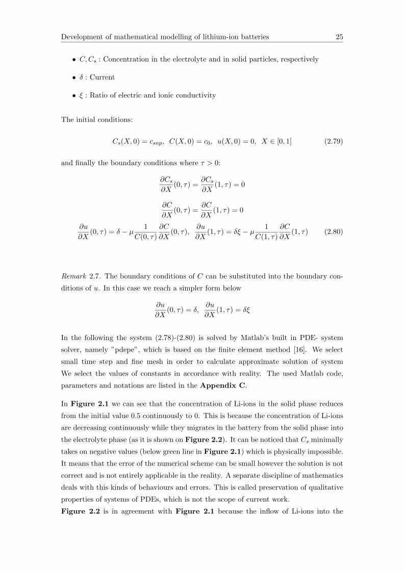
In Figure 2.1 we can see that the concentration of Li-ions in the solid phase reduces
from the initial value 0.5 continuously to 0. This is because the concentration of Li-ions
are decreasing continuously while they migrates in the battery from the solid phase into
the electrolyte phase (as it is shown on Figure 2.2). It can be noticed that Cs minimally
takes on negative values (below green line in Figure 2.1) which is physically impossible.
It means that the error of the numerical scheme can be small however the solution is not
correct and is not entirely applicable in the reality. A separate discipline of mathematics
deals with this kinds of behaviours and errors. This is called preservation of qualitative
properties of systems of PDEs, which is not the scope of current work.
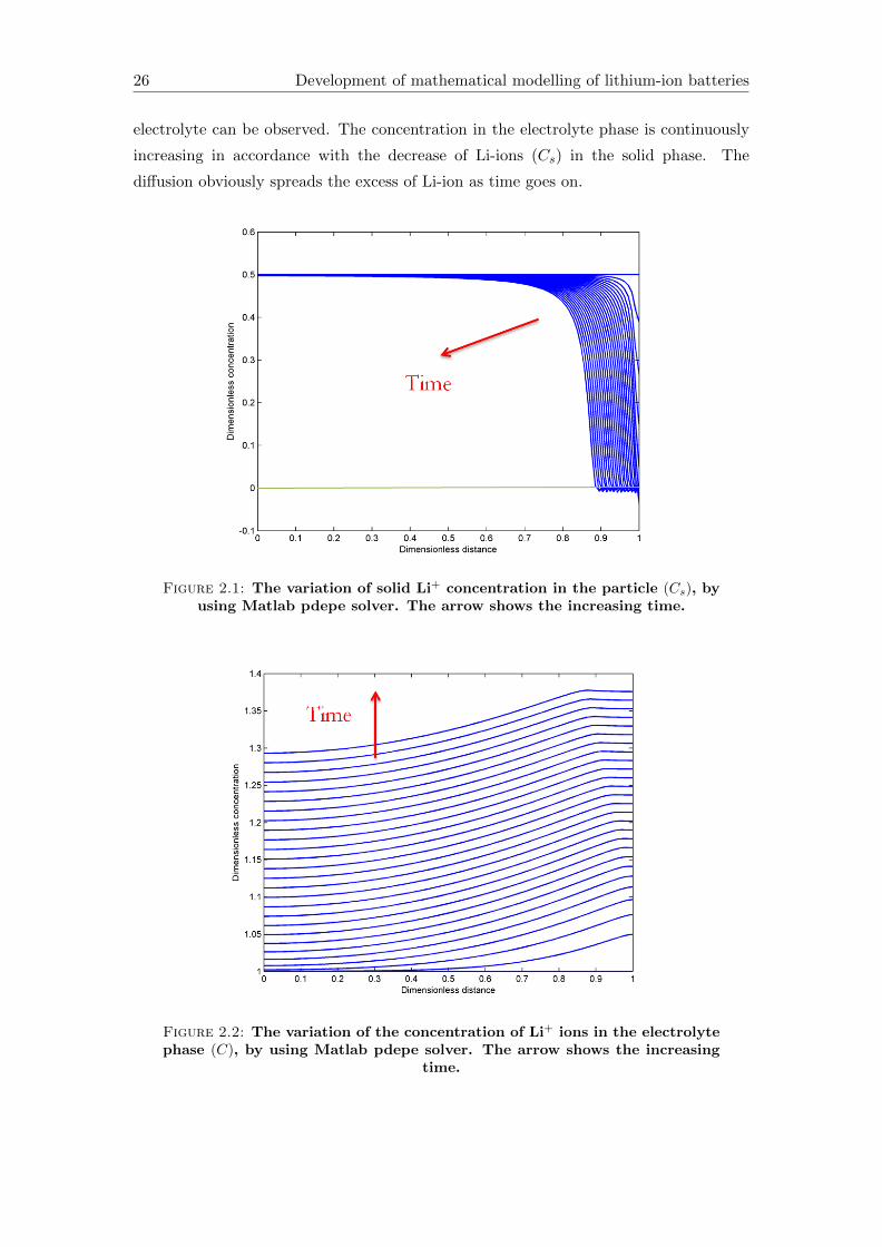
Figure 2.2 is in agreement with Figure 2.1 because the inflow of Li-ions into the
26 Development of mathematical modelling of lithium-ion batteries
electrolyte can be observed. The concentration in the electrolyte phase is continuously
increasing in accordance with the decrease of Li-ions (Cs) in the solid phase. The
diffusion obviously spreads the excess of Li-ion as time goes on.
Figure 2.1: The variation of solid Li+ concentration in the particle (Cs), byusing Matlab pdepe solver. The arrow shows the increasing time.
Figure 2.2: The variation of the concentration of Li+ ions in the electrolytephase (C), by using Matlab pdepe solver. The arrow shows the increasing
time.
Development of mathematical modelling of lithium-ion batteries 27
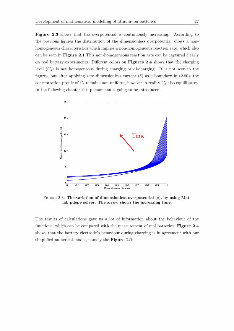
Figure 2.3 shows that the overpotential is continuously increasing. According to
the previous figures the distribution of the dimensionless overpotential shows a non-
homogeneous characteristics which implies a non-homogeneous reaction rate, which also
can be seen in Figure 2.1 This non-homogeneous reaction rate can be captured clearly
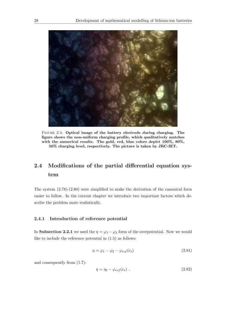
on real battery experiments. Different colors on Figures 2.4 shows that the charging
level (Cs) is not homogeneous during charging or discharging. It is not seen in the
figures, but after applying zero dimensionless current (δ) as a boundary in (2.80), the
concentration profile of Cs remains non-uniform, however in reality Cs also equilibrates.
In the following chapter this phenomena is going to be introduced.
Figure 2.3: The variation of dimensionless overpotential (u), by using Mat-lab pdepe solver. The arrow shows the increasing time.
The results of calculations gave us a lot of information about the behaviour of the
functions, which can be compared with the measurement of real batteries. Figure 2.4
shows that the battery electrode’s behaviour during charging is in agreement with our
simplified numerical model, namely the Figure 2.1.
28 Development of mathematical modelling of lithium-ion batteries
Figure 2.4: Optical image of the battery electrode during charging. Thefigure shows the non-uniform charging profile, which qualitatively matcheswith the numerical results. The gold, red, blue colors depict 100%, 80%,
50% charging level, respectively. The picture is taken by JRC-IET.
2.4 Modifications of the partial differential equation sys-
tem
The system (2.78)-(2.80) were simplified to make the derivation of the canonical form
easier to follow. In the current chapter we introduce two important factors which de-
scribe the problem more realistically.
2.4.1 Introduction of reference potential
In Subsection 2.2.1 we used the η = ϕ1−ϕ2 form of the overpotential. Now we would
like to include the reference potential in (1.5) as follows:
η = ϕ1 − ϕ2 − ϕref (cs) (2.81)
and consequently from (1.7):
η = η2 − ϕref (cs) . (2.82)
Development of mathematical modelling of lithium-ion batteries 29
Substituting (2.82) into (2.13):
− ∂
∂x
(κeff
∂ϕ2
∂x
)+
∂
∂x
[κeffRT
F
(1 +
∂ ln fA(c)
∂ ln c
)(1− t0+)
∂ ln c
∂x
]=
= an,pi0(cmax − cs)αn(cs)αp(c)αp ·
·[exp
(αnF
RT(η2 − ϕref (cs))
)− exp
(−αpFRT
(η2 − ϕref (cs))
) ]+an,pCdl
∂η2∂t
(2.83)
which can be rewritten in the following form:
− ∂
∂x
(κeff
∂ϕ2
∂x
)+
∂
∂x
[κeffRT
F
(1 +
∂ ln fA(c)
∂ ln c
)(1− t0+)
∂ ln c
∂x
]=
= an,pi0(cmax − cs)αn(cs)αp(c)αp2 sinh
(F
RT(η2 − ϕref (cs))
)+ an,pCdl
∂η2∂t
. (2.84)
If we apply the same steps such as in (2.16)-(2.67), then we reach the form:
∂u
∂τ(X, τ) =
∂2u
∂X2(X, τ) + µ
∂
∂X
(1
C(X, τ)
∂C
∂X(X, τ)
)−
− ν2(cmax − Cs(X, τ))Cs(X, τ)C(X, τ) sinh (u(X, τ)− Φ · ϕref (Cs(X, τ))) (2.85)
where
φ :=F
RT. (2.86)
Usually ϕref (Cs) can be approximated well by a linear function of Cs for example:
ϕref (Cs) ≈ A+BCs (2.87)
so (2.85) can be rewritten in the following form:
∂u
∂τ(X, τ) =
∂2u
∂X2(X, τ) + µ
∂
∂X
(1
C(X, τ)
∂C
∂X(X, τ)
)−
− ν2(cmax − Cs(X, τ))Cs(X, τ)C(X, τ) sinh (u(X, τ)− Φ[A+BCs(X, τ)]) (2.88)
and consequently the initial conditions need to be modified by the following way:
u(X, 0) = Φ · ϕref (Cs(X, 0)) = Φ · ϕref (csnp) = Φ(A+Bcsnp) (2.89)
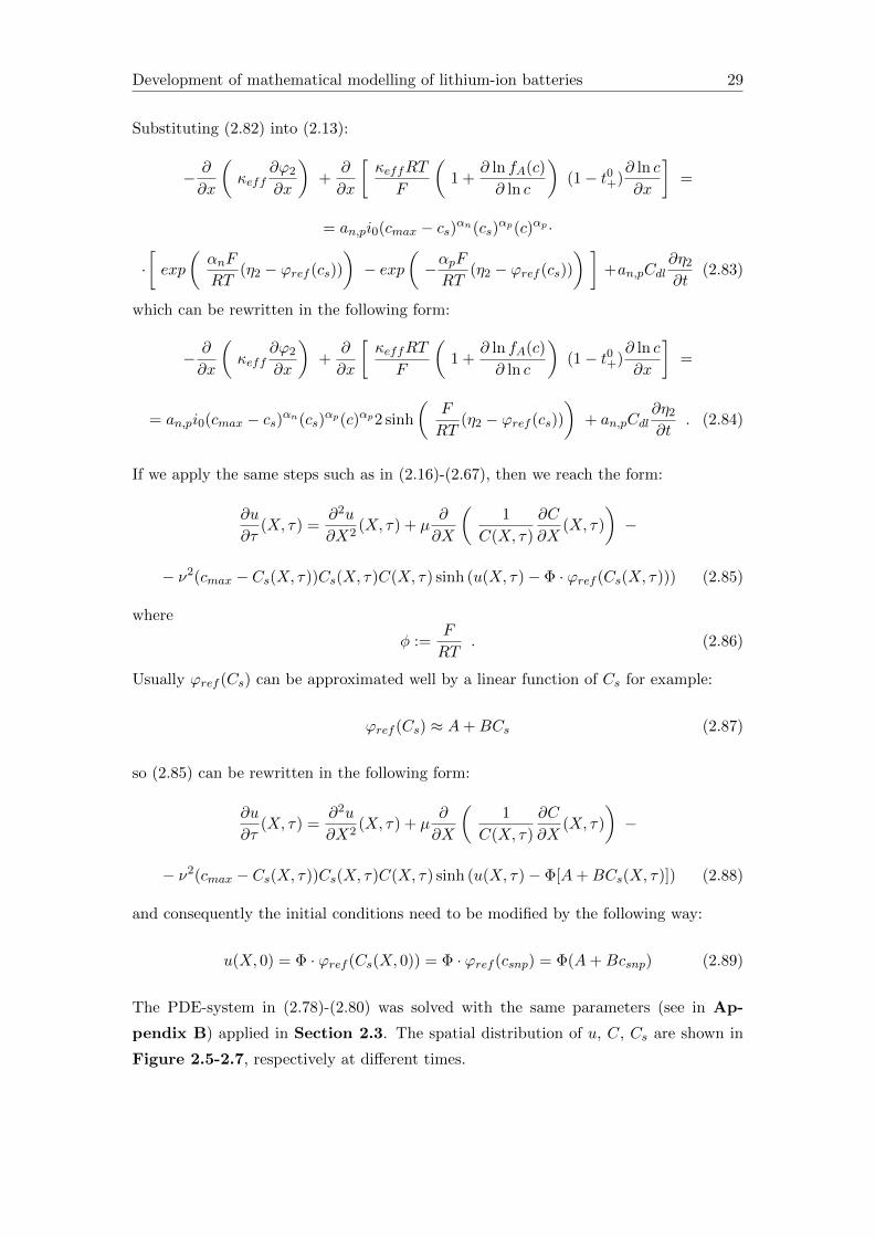
The PDE-system in (2.78)-(2.80) was solved with the same parameters (see in Ap-
pendix B) applied in Section 2.3. The spatial distribution of u, C, Cs are shown in
Figure 2.5-2.7, respectively at different times.
30 Development of mathematical modelling of lithium-ion batteries
Figure 2.5: The variation of solid Li+ concentration in the particle (Cs)with reference potential, by using Matlab pdepe solver. The arrow shows
the increasing time.
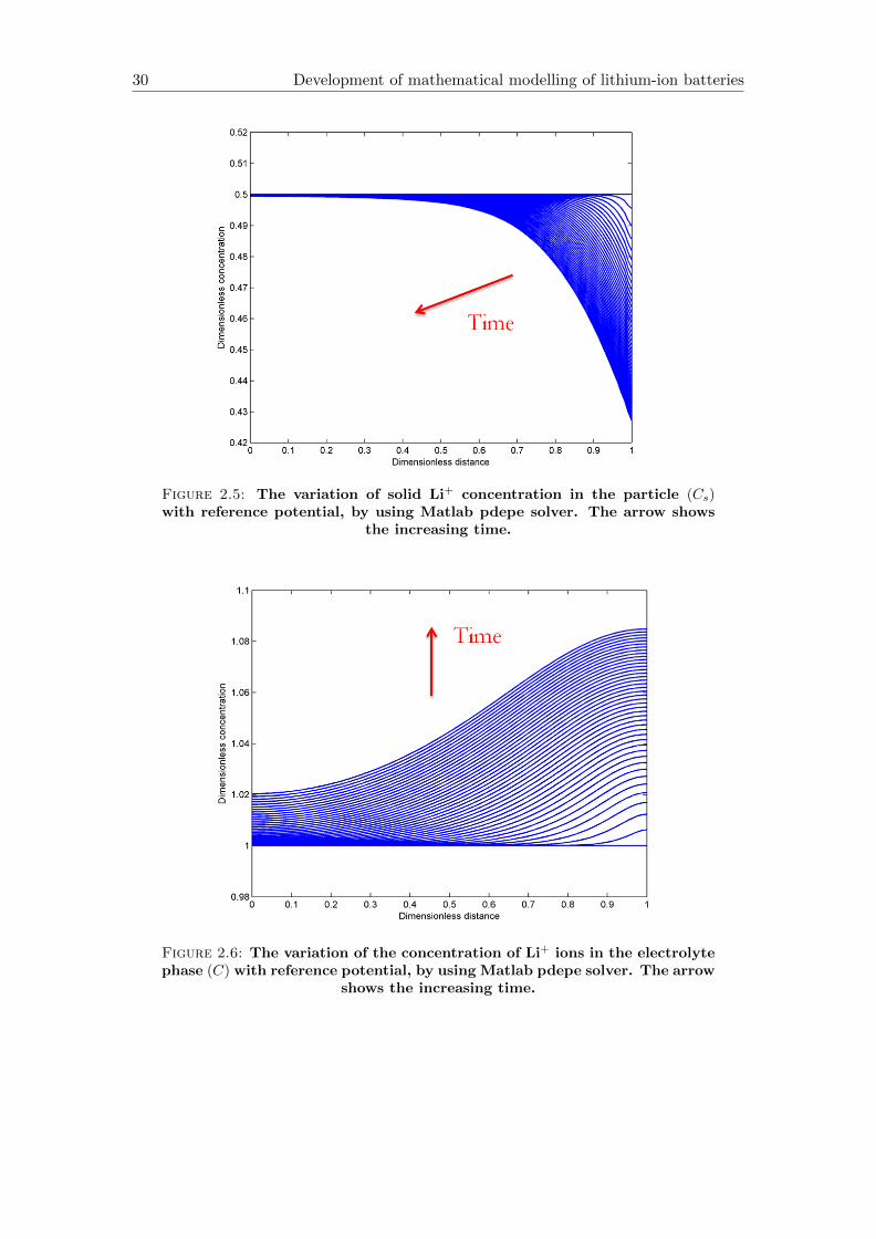
Figure 2.6: The variation of the concentration of Li+ ions in the electrolytephase (C) with reference potential, by using Matlab pdepe solver. The arrow
shows the increasing time.
Development of mathematical modelling of lithium-ion batteries 31
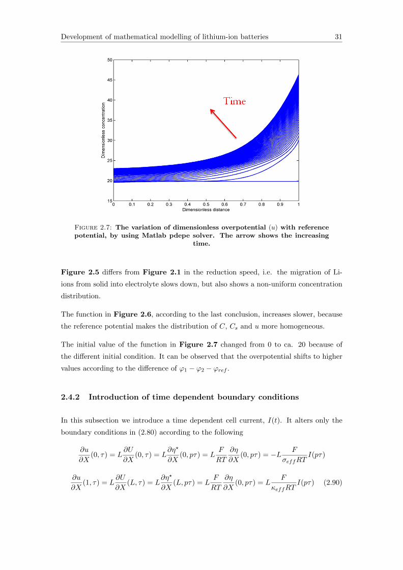
Figure 2.7: The variation of dimensionless overpotential (u) with referencepotential, by using Matlab pdepe solver. The arrow shows the increasing
time.
Figure 2.5 differs from Figure 2.1 in the reduction speed, i.e. the migration of Li-
ions from solid into electrolyte slows down, but also shows a non-uniform concentration
distribution.
The function in Figure 2.6, according to the last conclusion, increases slower, because
the reference potential makes the distribution of C, Cs and u more homogeneous.
The initial value of the function in Figure 2.7 changed from 0 to ca. 20 because of
the different initial condition. It can be observed that the overpotential shifts to higher
values according to the difference of ϕ1 − ϕ2 − ϕref .
2.4.2 Introduction of time dependent boundary conditions
In this subsection we introduce a time dependent cell current, I(t). It alters only the
boundary conditions in (2.80) according to the following
∂u
∂X(0, τ) = L
∂U
∂X(0, τ) = L
∂η?
∂X(0, pτ) = L
F
RT
∂η
∂X(0, pτ) = −L F
σeffRTI(pτ)
∂u
∂X(1, τ) = L
∂U
∂X(L, τ) = L
∂η?
∂X(L, pτ) = L
F
RT
∂η
∂X(0, pτ) = L
F
κeffRTI(pτ) (2.90)
32 Development of mathematical modelling of lithium-ion batteries
but pτ ≡ t, so the time variables are different, i.e.:
∂u
∂X(0, τ) = −L F
σeffRTI(t),
∂u
∂X(1, τ) = L
F
κeffRTI(t) (2.91)
So we have to introduce a new cell current whit a different time dependence:
I2(τ) := I(pτ) (2.92)
and consequently:
∂u
∂X(0, τ) = −L F
σeffRTI2(τ),
∂u
∂X(1, τ) = L
F
κeffRTI2(τ) (2.93)
In the following a step function is applied in the form
I2(τ) = a · χK(τ) (2.94)
where
χK(τ) = 1 if τ ∈ K, χK(τ) = 0 if τ /∈ K
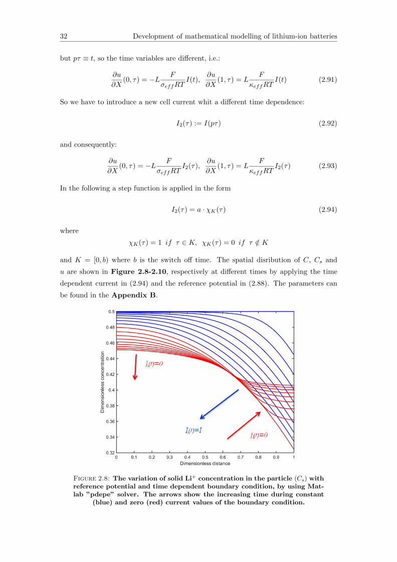
and K = [0, b) where b is the switch off time. The spatial disribution of C, Cs and
u are shown in Figure 2.8-2.10, respectively at different times by applying the time
dependent current in (2.94) and the reference potential in (2.88). The parameters can
be found in the Appendix B.
Figure 2.8: The variation of solid Li+ concentration in the particle (Cs) withreference potential and time dependent boundary condition, by using Mat-lab ”pdepe” solver. The arrows show the increasing time during constant
(blue) and zero (red) current values of the boundary condition.
Development of mathematical modelling of lithium-ion batteries 33
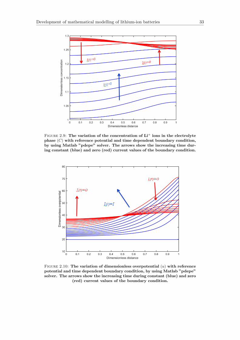
Figure 2.9: The variation of the concentration of Li+ ions in the electrolytephase (C) with reference potential and time dependent boundary condition,by using Matlab ”pdepe” solver. The arrows show the increasing time dur-ing constant (blue) and zero (red) current values of the boundary condition.
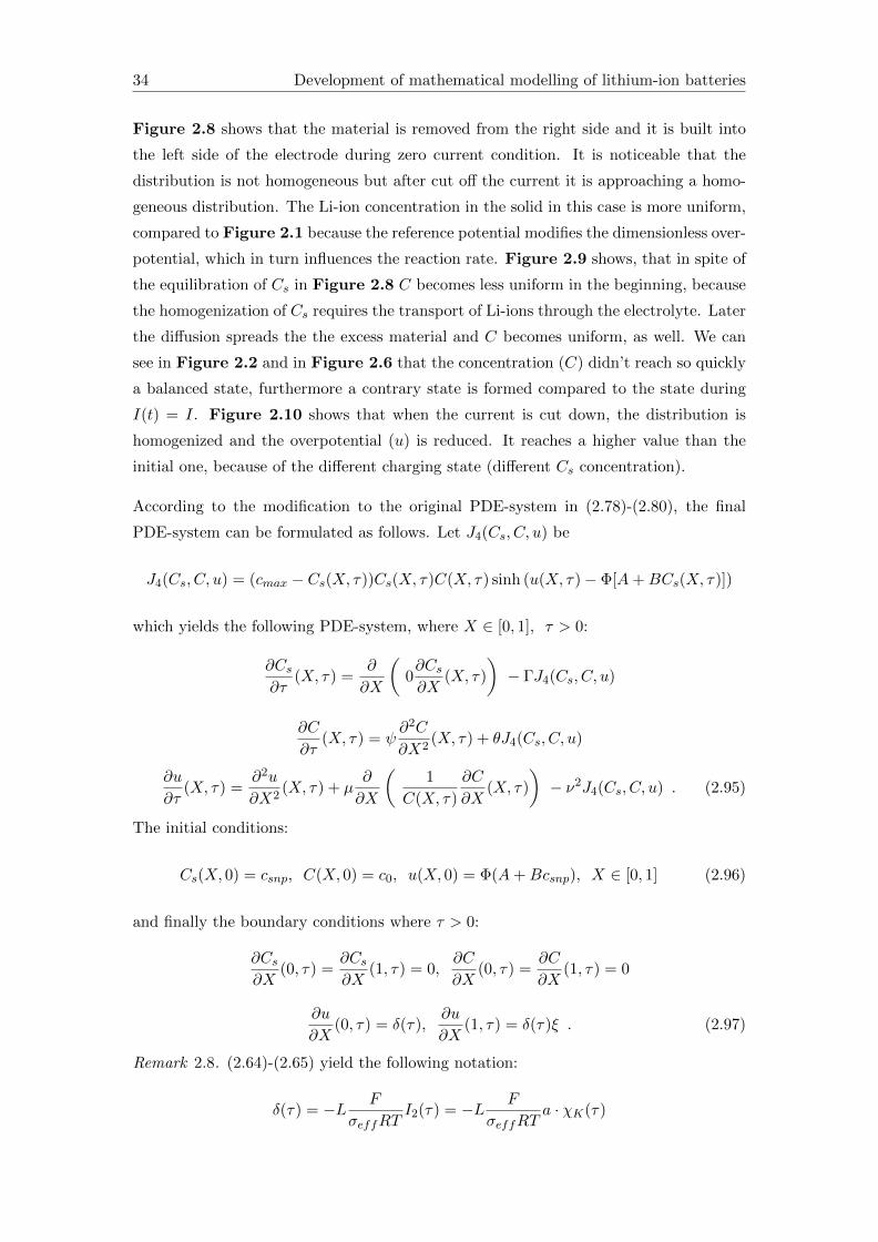
Figure 2.10: The variation of dimensionless overpotential (u) with referencepotential and time dependent boundary condition, by using Matlab ”pdepe”solver. The arrows show the increasing time during constant (blue) and zero
(red) current values of the boundary condition.
34 Development of mathematical modelling of lithium-ion batteries
Figure 2.8 shows that the material is removed from the right side and it is built into
the left side of the electrode during zero current condition. It is noticeable that the
distribution is not homogeneous but after cut off the current it is approaching a homo-
geneous distribution. The Li-ion concentration in the solid in this case is more uniform,
compared to Figure 2.1 because the reference potential modifies the dimensionless over-
potential, which in turn influences the reaction rate. Figure 2.9 shows, that in spite of
the equilibration of Cs in Figure 2.8 C becomes less uniform in the beginning, because
the homogenization of Cs requires the transport of Li-ions through the electrolyte. Later
the diffusion spreads the the excess material and C becomes uniform, as well. We can
see in Figure 2.2 and in Figure 2.6 that the concentration (C) didn’t reach so quickly
a balanced state, furthermore a contrary state is formed compared to the state during
I(t) = I. Figure 2.10 shows that when the current is cut down, the distribution is
homogenized and the overpotential (u) is reduced. It reaches a higher value than the
initial one, because of the different charging state (different Cs concentration).
According to the modification to the original PDE-system in (2.78)-(2.80), the final
PDE-system can be formulated as follows. Let J4(Cs, C, u) be
J4(Cs, C, u) = (cmax − Cs(X, τ))Cs(X, τ)C(X, τ) sinh (u(X, τ)− Φ[A+BCs(X, τ)])
which yields the following PDE-system, where X ∈ [0, 1], τ > 0:
∂Cs∂τ
(X, τ) =∂
∂X
(0∂Cs∂X
(X, τ)
)− ΓJ4(Cs, C, u)
∂C
∂τ(X, τ) = ψ
∂2C
∂X2(X, τ) + θJ4(Cs, C, u)
∂u
∂τ(X, τ) =
∂2u
∂X2(X, τ) + µ
∂
∂X
(1
C(X, τ)
∂C
∂X(X, τ)
)− ν2J4(Cs, C, u) . (2.95)
The initial conditions:
Cs(X, 0) = csnp, C(X, 0) = c0, u(X, 0) = Φ(A+Bcsnp), X ∈ [0, 1] (2.96)
and finally the boundary conditions where τ > 0:
∂Cs∂X
(0, τ) =∂Cs∂X
(1, τ) = 0,∂C
∂X(0, τ) =
∂C
∂X(1, τ) = 0
∂u
∂X(0, τ) = δ(τ),
∂u
∂X(1, τ) = δ(τ)ξ . (2.97)
Remark 2.8. (2.64)-(2.65) yield the following notation:
δ(τ) = −L F
σeffRTI2(τ) = −L F
σeffRTa · χK(τ)

Chapter 3
Solution of the model and the
results
3.1 Solution of the partial differential equation system by
operator splitting
After we introduced the foundation of splitting algorithm in Section 1.2, we can adapt it
to our problem, namely to the system (2.95)-(2.97). Let’s define ~w(x, t) as the following:
~w(x, t) := [Cs C u]T (x, t) . (3.1)
The (2.95) PDE-system can be rewritten in matrix form as follows:
∂ ~w
∂t=
0 0 0
0 ψ ∂2
∂x20
0 0 ∂2
∂x2
·Cs
C
u
+
−ΓJ4
θJ4
µ∂2 lnC(x,t)∂x2
− ν2J4
(3.2)
or with simplifed notation:∂ ~w
∂t= A · ~w + f (3.3)
where
A =
0 0 0
0 ψ ∂2
∂x20
0 0 ∂2
∂x2
, f =
−ΓJ4
θJ4
µ∂2 lnC(x,t)∂x2
− ν2J4
35
Results
With the proper the initial and the boundary conditions:
~w(x, 0) := ~w0 =
Cs
C
u
(x, 0) =
csnp
c0
Φ(A+Bcsnp)
, x ∈ [0, 1]
∂ ~w
∂x(0, t) =
0
0
δ(t)
, ∂ ~w
∂x(1, t) =
0
0
δ(t)ξ
, 0 < t < τ (3.4)
So the sub-tasks can be prescribed as follows:
∂ ~w1
∂t= A · ~w1 (3.5)
∂ ~w2
∂t= f (3.6)
and the appropriate initial conditions are:
~w1(x, 0) := ~w0, ~w2(x, 0) := ~w1(x, τ) (3.7)
Now (3.5) and (3.6) match to Problem 1 and Problem 2 in Section1.2, consequently
the sequential splitting in Section1.2 can be applied on them. In the following these
vectors are calculated by analytical and by numerical methods. We will show that in
terms of applicability only one method provide useful results.
3.1.1 Analytical solution of the splitted problems
In this subsection we try to solve the (2.95)-(2.97) PDE-system an analytical way by
using sequential splitting [12]. It is shown in this section that the PDE-system can be
solved analytically, however the mesh functions can be calculated only by infinite series.
The calculation of the solution requires numerical program, which have usually very long
running time. The methods is solved by the steps A-B described below.
Step A, Solid Li+ concentration in the particle (Cs), Problem 1
∂C(1)s,1
∂t(x, t) = 0, 0 ≤ t ≤ τ, 0 ≤ x ≤ 1
C(1)s,1 (x, 0) = csnp,
∂C(1)s,1
∂x(0, t) =
∂C(1)s,1
∂x(1, t) = 0 . (3.8)
Results 37
Because this problem isn’t dependent on x, it can be solved easily by the integration of
t:
∫∂C
(1)s,1
∂t(x, t)dt =
∫0dt =⇒ C
(1)s,1 (x, t) + c1(x) = c2(x) =⇒ C
(1)s,1 (x, t) = c3(x)
where c1(x), c2(x) are appropriate space dependent constants and c3(x) = c2(x)− c1(x)
which is equal to csnp because the initial condition. Naturally this has the same value
in every time step (because it is not depend on t), so the solution of (3.8) at t = τ :
C(1)s,1 (x, τ) = csnp . (3.9)
Step B, Concentration of Li+ ions in the electrolyte phase (C), Problem 1
∂C(1)1
∂t(x, t) = ψ
∂2C(1)1
∂x2(x, t), 0 ≤ t ≤ τ, 0 ≤ x ≤ 1
C(1)1 (x, 0) = c0,
∂C(1)1
∂x(0, t) =
∂C(1)1
∂x(1, t) = 0 . (3.10)
By analytical way we seek the solution in the following form:
C(1)1 (x, t) = K(x)M(t) (3.11)
where K(x) and M(t) are unknown non-zero functions. So if we fit (3.10) to (3.11), we
reach:
M ′(t)K(x) = ψK ′′(x)M(t)
and after re-arrangement:
ψK ′′(x)
K(x)=M ′(t)
M(t).
Because the left side is dependent only on x and the right side is dependent only on
t, then the equation is hold only when both sides are constant, therefore the following
equation can be applied:
∃φ ∈ R : ψK ′′(x)
K(x)=M ′(t)
M(t)= φ (3.12)
and we reach:
ψK ′′(x) = φK(x), x ∈ (0, 1) . (3.13)
If we substitute (3.11) to the boundary conditions in (3.10), we reach:
M(t)∂K
∂x(0) = M(t)
∂K
∂x(1) = 0 =⇒ ∂K
∂x(0) =
∂K
∂x(1) = 0 . (3.14)
38 Results
For the easier calculation let λ be:
λ := −φψ.
Because (3.13) is an ordinary differential equation with constant coefficient, the solutions
of Eq(3.12) are the roots of the following characteristic polynomial:
ρ2 + λ = 0 . (3.15)
Depending on the sign of λ the following cases can be considered:
• If λ < 0, then the roots are real so the general solution of equation can be written
into the following form:
K(x) = c1e√−λx + c2e
−√−λx
where c1, c2 are appropriate constants. Using boundary conditions in Eq(3.14), we
reach:
c1√−λ− c2
√−λ = 0 =⇒ K(x) = c1
(e√−λx + e−
√−λx)
c1√−λ(e√−λx + e−
√−λx)
= 0⇐⇒ c1 = 0
which yields a not allowed K(x) = 0 equality.
• If λ = 0, then (3.12) has the form −K ′′(x) = 0 which is only met in case of the
following equality:
K(x) = c1X − c2
which yields such as in the previous case the not allowed K(x) = 0 equality.
• If λ > 0, then the roots are ±i√λ so the solution is:
K(x) = c1 sin( √
λx)
+ c2cos( √
λx)
where c1, c2 are appropriate constants. Using boundary conditions in (3.14), we
reach:
c1√λ cos (0)− c2
√λ sin (0) = 0 =⇒ c1
√λ = 0 =⇒ c1 = 0
c1√λ cos
( √λ)− c2√λ sin
( √λ)
= 0 =⇒ −c2√λ sin
( √λ)
= 0⇐⇒ λl = l2π2
which fulfills the original problem in (3.12) where l = 0, 1, 2, . . . .
Results 39
In summary the solution of (3.13) is:
Kl(x) = cl,1 cos (lπx), l = 0, 1, 2, . . . (3.16)
where cl,1 is an arbitrary constant. Now we can determine M(t) function using the
re-arranged form of (3.12):
M ′(t) = φM(t) = −λψM(t), t ∈ [0, τ ]
where λ = λk, which result the following solution:
Ml(t) = cl,2e−λψ t = cl,2e
−l2π2ψ t (3.17)
where cl,2 is an arbitrary constant. Substitute (3.16) and (3.17) to (3.11) we reach:
C(1)l,1 (x, t) = cl cos (lπx)e−l
2π2ψ t, l = 0, 1, 2, . . . (3.18)
where cl = cl,1cl,2 and consequently the summed values of this functions yields the
solution of (3.10):
C(1)1 (x, t) =
∞∑l=0
C(1)l,1 (x, t) =
∞∑l=0
cl cos (lπx)e−l2π2ψ t, l = 0, 1, 2, . . . . (3.19)
We need to define the values of cl, (l = 0, 1, 2, . . . ). By using the initial condition we
can conclude the following:
∞∑l=0
C(1)l,1 (x, 0) =
∞∑l=0
cl cos (lπx) = c0(x) = c0
Furthermore the Fourier-series of c0 equals to:
c0 =∞∑k=0
ck0 cos (kπx)
where
ck0 =1
2
∫ 1
−1c0 cos (kπu) du =
1
2c0
∫ 1
−1cos (kπu) du.
In summary, if we choose cl = ck0 than we reach the solution of the (3.10) PDE:
C(1)1 (x, t) =
∞∑l=0
cl0 cos (lπx)e−l2π2ψ t . (3.20)
It can be obtained that Problem 1 of splitting method yields an infinite series of func-
tions (cosinus, exponential) for C. In Problem 2 of the method the initial conditions
40 Results
are (3.20) at t = τ which solution have an infinite series as well. This solution at t = τ
is the initial condition of Problem 1 of splitting method etc.. It can be concluded that
the analytical calculation is long and complicated in case of small step sizes (in this case
the number of steps are big). The code for the analytical solution was developed, but it
was found that the running time is very long even at few number of steps. In practice
we have to find an other way to solve the PDE-system (2.95)-(2.97), which is described
in the following chapter.
3.1.2 Numerical solution of the splitted problems
In this subsection we apply FDM for the solution of (2.95)-(2.97) PDE-system. This
method is based on the calculation of finite difference approximations of derivatives.
The methods is solved by the steps A-F described below.
Step A, Solid Li+ concentration in the particle (Cs), Problem 1
∂C(1)s,1
∂t(x, t) = 0, 0 ≤ t ≤ τ, 0 ≤ x ≤ 1
C(1)s,1 (x, 0) = csnp,
∂C(1)s,1
∂x(0, t) =
∂C(1)s,1
∂x(1, t) = 0 . (3.21)
This approach always gives a solution which equals to the initial condition at the end
of each time interval, i.e. the solution at t = τ :
C(1)s,1 (x, τ) = csnp(x) = csnp (3.22)
Remark 3.1. In the first step (3.22) doesn’t depend on x but in the further steps it
became space (x) dependent.
Step B, Concentration of Li+ ions in the electrolyte phase (C), Problem 1
∂C(1)1
∂t(x, t) = ψ
∂2C(1)1
∂x2(x, t), 0 ≤ t ≤ τ, 0 ≤ x ≤ 1
C(1)1 (x, 0) = c0,
∂C(1)1
∂x(0, t) =
∂C(1)1
∂x(1, t) = 0 . (3.23)
Now we introduce the following linear operator:
Lw(x, t) =
(∂w
∂t− ψ∂
2w
∂x2
)(x, t), (x, t) ∈ (0, 1)× (0, τ ] (3.24)
Results 41
and the following function:
f(x, t) =
f(x, t) if x ∈ 0, 1 or t = 0
0 else(3.25)
which is actually beseemed for initial and boundary conditions. Using this notations,
the equation system can be modified to the following form:
LC(1)1 (x, t) = f(x, t) (3.26)
Let∐
(ωh,τ ) be a vector space defined on the ωh,τ mesh points (see the definition of it in
Section 1.2). Our aim is to find a yh,τ ∈∐
(ωh,τ ) function which is close to C(1)1 in the
ωh,τ mesh points. So the task is to give an Lh,τ :∐
(ωh,τ )→∐
(ωh,τ ) operator,where:
ωh,τ :=
(xi, tn);xi = ih; tn = nτ ;h =
1
Nx; τ =
T
NT; i = 0, 1, . . . , Nx;n = 0, 1, . . . , NT
and to give a bh,τ element of
∐(ωh,τ ) which satisfys the following equation:
Lh,τyh,τ = bh,τ .
Lh,τ is chosen to satisfy the following lemma’s conditions [12]:
Lemma 3.2. For arbitrary γ ∈ [0, 1] number and by sufficiently smooth y(x, t) function
the relations
∂y
∂t(xi, tn−1 + γτ) =
y(xi, tn−1 + τ)− y(xi, tn−1)
τ+O(τ)
∂2y
∂x2(xi, tn−1 + γτ) =
y(xi+1, tn−1)− 2y(xi, tn−1) + y(xi−1, tn−1)
h2+O(τ + h2)
hold.
Our goal is to give the approximation for the value of (Lh,τyh,τ )(xi, tn) with accuracy
O(τ + h2) using the value of y function in the mesh points. Let’s define the following
operator:
(Lh,τyh,τ )(xi, tn) =yni − y
n−1i
τ− ψ
yni+1 − 2yni + yni−1h2
if (xi, tn) ∈ ωh,τ (3.27)
where yni = yh,τ (xi, tn), and consequently (3.23) can be rewritten to:
yni − yn−1i
τ− ψ
yni+1 − 2yni + yni−1h2
= bni . (3.28)
42 Results
We know the values of function C only on the parabolic boundary, so we have to ap-
proximate it on the (xi, tn) ∈ ωh,τ meshpoints.
Remark 3.3. In order to reach convergence the relation τh2≤ 0.5 should be satisfied [12].
Re-arrangement of (3.28) yields:
1
τyn−1i − ψ 1
h2yni−1 − ψ
1
h2yni+1 +
(ψ
2
h2+
1
τ
)yni = bni
i = 1, 2, . . . , Nx − 1, n = 1, 2, . . . , NT
which is equivalent to
yn−1i − qyni−1 − qyni+1 + ( 2q + 1) yni = τbni (3.29)
where q = ψ τh2
. The corresponding initial and boundary conditions are:
y0i = c0, i+ 0, 1, . . . , Nx
yn1 − yn0h
=ynNx− ynNx
h= 0, n = 1, 2, . . . , NT (3.30)
according to (3.23). Let yn, f ∈ R(Nx+1) and Eh, Bh ∈ R(Nx+1)(Nx+1) be:
yn :=[yn0 . . . y
nNx
]T , Eh := Ih identity matrix
Bh :=
−1 +1 0 . . . 0 0 0
−q 2q + 1 −q . . . 0 0 0
· · · · · · ·
· · · · · · ·
· · · · · · ·
0 0 0 . . . −q 2q + 1 −q
0 0 0 . . . 0 −1 1
, f(yn−1) =
0 · h
yn−11
·
·
·
yn−1Nx−1
0 · h
(3.31)
Apply notations in (3.31), the equation-system (3.29) can be rewritten in the following
form:
Eh · y0 = [c0 . . . c0]T ∈ R(Nx+1), Bh · yn = f(yn−1), n = 1, 2, . . . , NT . (3.32)
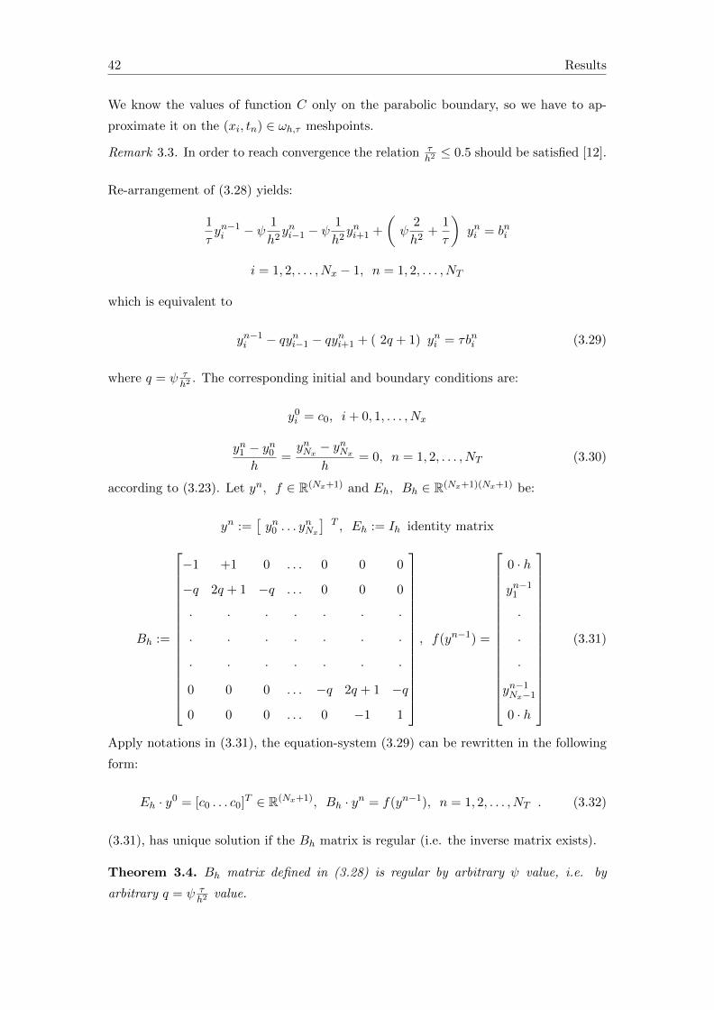
(3.31), has unique solution if the Bh matrix is regular (i.e. the inverse matrix exists).
Theorem 3.4. Bh matrix defined in (3.28) is regular by arbitrary ψ value, i.e. by
arbitrary q = ψ τh2
value.
Results 43
Proof:
We applied the approach of Horn et al. [17] to proof it for our special case. At first we
introduce the following definitions:
Definition 3.5. The directed graph of A ∈ Rn×n is the directed graph on n nodes
1, 2, . . . , n such that there is a directed arc in the graph from i to j if and only if
ai,j 6= 0.
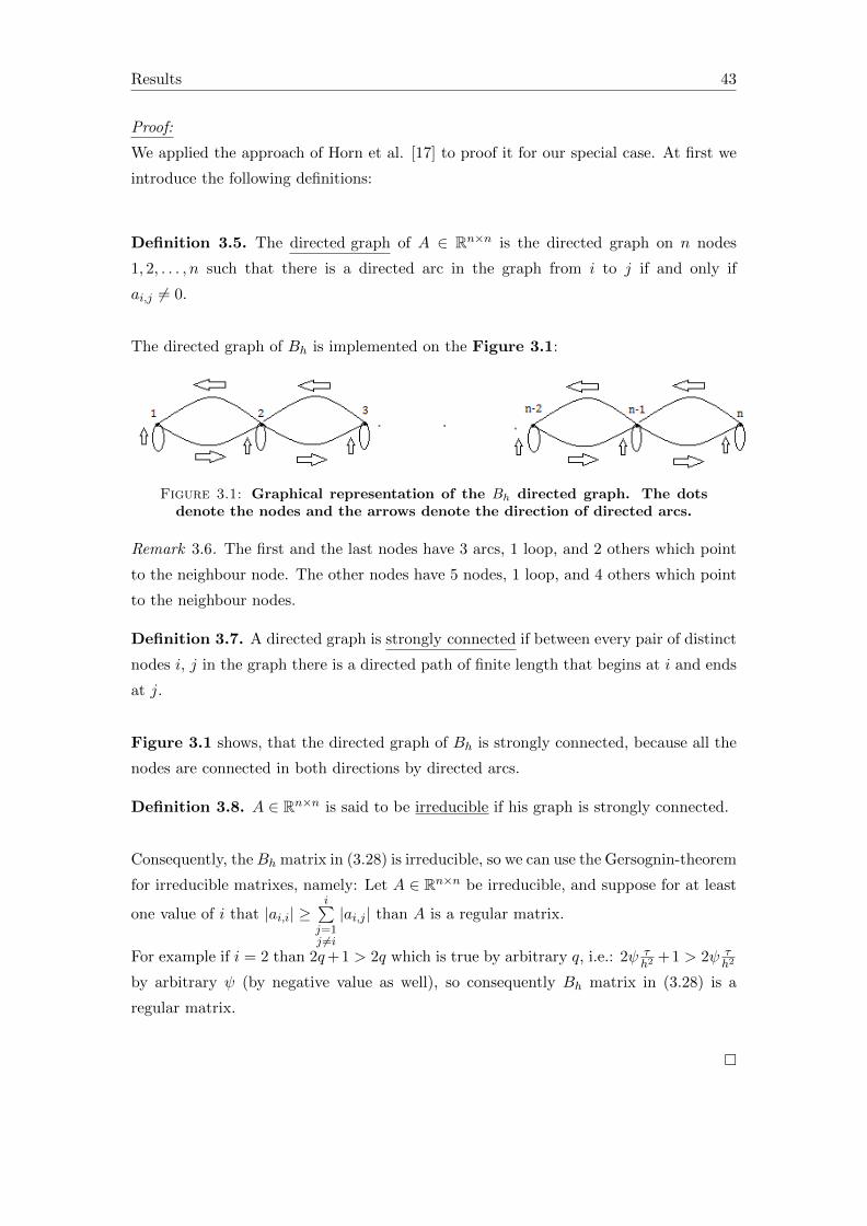
The directed graph of Bh is implemented on the Figure 3.1:
Figure 3.1: Graphical representation of the Bh directed graph. The dotsdenote the nodes and the arrows denote the direction of directed arcs.
Remark 3.6. The first and the last nodes have 3 arcs, 1 loop, and 2 others which point
to the neighbour node. The other nodes have 5 nodes, 1 loop, and 4 others which point
to the neighbour nodes.
Definition 3.7. A directed graph is strongly connected if between every pair of distinct
nodes i, j in the graph there is a directed path of finite length that begins at i and ends
at j.
Figure 3.1 shows, that the directed graph of Bh is strongly connected, because all the
nodes are connected in both directions by directed arcs.
Definition 3.8. A ∈ Rn×n is said to be irreducible if his graph is strongly connected.
Consequently, theBh matrix in (3.28) is irreducible, so we can use the Gersognin-theorem
for irreducible matrixes, namely: Let A ∈ Rn×n be irreducible, and suppose for at least
one value of i that |ai,i| ≥i∑
j=1j 6=i
|ai,j | than A is a regular matrix.
For example if i = 2 than 2q+1 > 2q which is true by arbitrary q, i.e.: 2ψ τh2
+1 > 2ψ τh2
by arbitrary ψ (by negative value as well), so consequently Bh matrix in (3.28) is a
regular matrix.
44 Results
Because the inverse of Bh exist, we can rewrite (3.29)-(3.30) to the following form:
y0 = [c0 . . . c0]T , yn = B−1h · f(yn−1), n = 1, 2, . . . , NT (3.33)
and with this explicit formula we can take the different values of function in mesh points
which yields the finally form of solution at t = τ :
C(1)1 (xi, τ) = yNT
i , i = 0, 1, . . . , Nx . (3.34)
which is in compliance with Problem 1 of splitting method.
Step C, Dimensionless overpotential (u), Problem 1
∂u(1)1
∂t(x, t) =
∂2u(1)1
∂x2(x, t), 0 ≤ t ≤ τ, 0 ≤ x ≤ 1
u(1)1 (x, 0) = Φ(A+Bcsnp) := u0,
∂u(1)1
∂x(0, t) = δ(t),
∂u(1)1
∂x(1, t) = δ(t)ξ (3.35)
We can use the same process described in step B, and we reach (by using the notation
u(1)1 (xi, tn) = yni ) the following equation-system:
y0 = [u0 . . . u0]T , yn = B−1h · f(yn−1), n = 1, 2, . . . , NT (3.36)
where the value of q in Bh matrix is equal to τh2
and furthermore:
f(yn−1) = [hδ(t) yn−11 . . . yn−1Nx−1 hδ(t)ξ]T .
The boundary and initial conditions are:
y0i = u0, i = 0, 1, . . . , Nx
yn1 − yn0h
= δ(t),ynNx− ynNx
h= δ(t)ξ, n = 1, 2, . . . , NT . (3.37)
Consequently, the final solution of (3.35) at t = τ is the following:
u(1)1 (xi, τ) = yNT
i , i = 0, 1, . . . , Nx . (3.38)
Step D, Solid Li+ concentration in the particle (Cs), Problem 2
Remark 3.9. The solution of step A, namely (3.22) is used as the initial condition of
this problem which is actually an explicit method.
Results 45
∂C(1)s,2
∂t(x, t) = −ΓJ4(C
?s , C
?, u?), 0 ≤ t ≤ τ
C(1)s,2 (x, 0) = csnp, ∆? := ∆(1)(x, τ), ∆ ∈ Cs, C, u (3.39)
First we determine the functions including J4:
C?s = C(1)s,1 (xi, τ) = csnp, C
? = C(1)1 (xi, τ) = yNT
i
u? = u(1)1 (xi, τ) = yNT
i
Substitute this values in J4, we reach the following equation:
∂C(1)s,2
∂t(x, t) = −Γ(cmax − csnp)csnpyNT
i sinh (yNTi − Φ[A+Bcsnp]) . (3.40)
Let Ξi define as following:
Ξi := −Γ(cmax − csnp)csnpyNTi sinh (yNT
i − Φ[A+Bcsnp]) (3.41)
and let’s define the following Lh,τ :∐
(ωh,τ )→∐
(ωh,τ ) operator:
(Lh,τwh,τ )(xi, tn) =wni − w
n−1i
τ. (3.42)
where let wni the approximation of Cs in the (xi, tn) mesh point. Substitute (3.40) and
(3.41) into (3.42), we reach:wni − w
n−1i
τ= Ξi . (3.43)
After a simple re-arrangement we get the following equation-system:
wni = Ξiτ + wn−1i , n = 1, 2, . . . , NT (3.44)
from where we can calculate the solution on the ωh,τ mesh, and we reach at t = τ the
following:
C(1)s,2 (xi, τ) = wNT
i . (3.45)
Step E, Concentration of Li+ ions in the electrolyte phase (C), Problem 2
Remark 3.10. The solution of step B, namely (3.34) is used as the initial condition of
this problem.
∂C(1)2
∂t(x, t) = θJ4(C
?s , C
?, u?), 0 ≤ t ≤ τ
C(1)2 (x, 0) = yNT
i , ∆? := ∆(1)(x, τ), ∆ ∈ Cs, C, u (3.46)
46 Results
We follow the same steps such as in step D, so (3.46) can be rewritten in the following
form:
∂C(1)2
∂t(x, t) = θ(cmax − csnp)csnpyNT
i sinh (yNTi − Φ[A+Bcsnp]) . (3.47)
Let Θi define as following:
Θi := θ(cmax − csnp)csnpyNTi sinh (yNT
i − Φ[A+Bcsnp]) (3.48)
and let’s define the following Lh,τ :∐
(ωh,τ ) →∐
(ωh,τ ) operator and notation
C(1)2 (xi, tn) = wni as well:
(Lh,τ wh,τ )(xi, tn) =wni − w
n−1i
τ(3.49)
and substitution of (3.48) and (3.49) in (3.47) yields:
wni − wn−1i
τ= Θi (3.50)
and after re-arrangement we reach finally the resolvable equation-system:
wni = Θiτ + wn−1i , n = 1, 2, . . . , NT (3.51)
which yields actually the solution of (3.46) at t = τ , namely:
C(1)2 (xi, τ) = wNT
i . (3.52)
Step F, Dimensionless overpotential (u), Problem 2
Remark 3.11. The solution of step C, namely (3.38) is used as the initial condition of
this problem.
∂u(1)2
∂t(x, t) = µ
∂2 lnC?
∂x2− ν2J4(C?s , C?, u?), 0 ≤ t ≤ τ
u(1)2 (x, 0) = yNT
i , ∆? := ∆(1)(x, τ), ∆ ∈ Cs, C, u (3.53)
In this problem we deal first with the first part of the source term. Applying the chain-
rule on ∂2 lnC?
∂x2yields the following form:
∂2 lnC?
∂x2(x, t) = − 1
C?2(x, t)+
1
C?(x, t)
∂2C?
∂x2(x, t) . (3.54)
Results 47
Let Lh,τ :∐
(ωh,τ ) →∐
(ωh,τ ) define the following operator by using the notation in
(3.34):
(Lh,τyh,τ )(xi, τ) =yNTi+1 − 2yNT
i + yNTi−1
h2(3.55)
where yNTi 6= 0 is the same as in the step B. Substitute (3.55) to (3.54) we reach:
− 1
(yNTi )2
+1
yNTi
(yNTi+1 − 2yNT
i + yNTi−1
h2
), i = 1, 2, . . . , Nx − 1 . (3.56)
We need this form only at t = τ so from combination of (3.54) and (3.56) we reach:
∂2 lnC?
∂x2(xi, τ) = − 1
(yNTi )2
+1
yNTi
(yNTi+1 − 2yNT
i + yNTi−1
h2
), i = 1, 2, . . . , Nx − 1 .
(3.57)
This form has complication only at the boundary (if i = 0 or i = Nx), so we have to
define two more forms, namely:
∂2 lnC?
∂x2(x0, τ) = − 1
(yNT0 )2
+1
yNT0
(yNT1 − yNT
0
h
)(3.58)
and∂2 lnC?
∂x2(xNx , τ) = − 1
(yNTNx
)2+
1
yNTNx
(yNTNx− yNT
Nx−1h
). (3.59)
Let Pi be:
Pi =
µ
[− 1
(yNTNx
)2+ 1
yNTNx
(yNTi+1−2y
NTi +y
NTi−1
h2
) ]− ν2J4(C?s , C?, u?) if i = 1, . . . Nx − 1
µ
[− 1
(yNTNx
)2+ 1
yNTNx
(yNTi+1−y
NTi
h
) ]− ν2J4(C?s , C?, u?) if i = 0
µ
[− 1
(yNTNx
)2+ 1
yNTNx
(yNTi −yNT
i−1
h
) ]− ν2J4(C?s , C?, u?) if i = Nx
(3.60)
and by using the u(1)2 (xi, tn) = ˜wni notation, we reach after re-arrangement the resolvable
equation-system:
˜wni = Piτ + ˜wn−1i (3.61)
which yields actually the solution of (3.53) at t = τ :
u(1)2 (xi, τ) = ˜wNT
i . (3.62)
When we follow this process iteratively according to the Problem 1 and Problem 2
in Section 1.2, we reach the solution of (2.95)-(2.97) PDE-system in different points
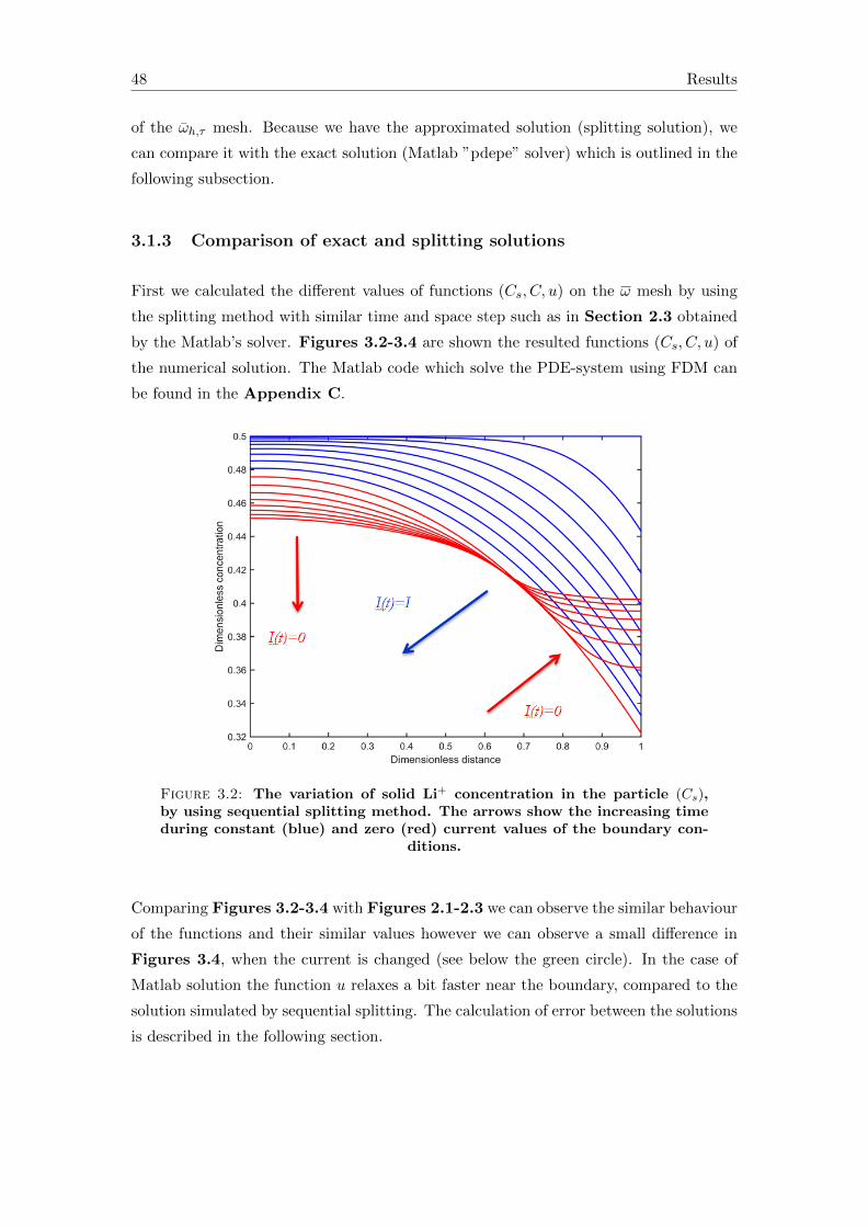
48 Results
of the ωh,τ mesh. Because we have the approximated solution (splitting solution), we
can compare it with the exact solution (Matlab ”pdepe” solver) which is outlined in the
following subsection.
3.1.3 Comparison of exact and splitting solutions
First we calculated the different values of functions (Cs, C, u) on the ω mesh by using
the splitting method with similar time and space step such as in Section 2.3 obtained
by the Matlab’s solver. Figures 3.2-3.4 are shown the resulted functions (Cs, C, u) of
the numerical solution. The Matlab code which solve the PDE-system using FDM can
be found in the Appendix C.
Figure 3.2: The variation of solid Li+ concentration in the particle (Cs),by using sequential splitting method. The arrows show the increasing timeduring constant (blue) and zero (red) current values of the boundary con-
ditions.
Comparing Figures 3.2-3.4 with Figures 2.1-2.3 we can observe the similar behaviour
of the functions and their similar values however we can observe a small difference in
Figures 3.4, when the current is changed (see below the green circle). In the case of
Matlab solution the function u relaxes a bit faster near the boundary, compared to the
solution simulated by sequential splitting. The calculation of error between the solutions
is described in the following section.

Results 49
Figure 3.3: The variation of the concentration of Li+ ions in the electrolytephase (C), by using sequential splitting method. The arrows show the in-creasing time during constant (blue) and zero (red) current values of the
boundary conditions.
Figure 3.4: The variation of dimensionless overpotential (u), by using se-quential splitting method. The arrows show the increasing time duringconstant (blue) and zero (red) current values of the boundary conditions.The green circle shows the location of the dissimilar behaviour of u compare
Figure 2.1.
50 Results
3.2 Accuracy of the splitting solution
Because of the exact solution is not known the splitting accuracy is expressed as the
relative error between the Matlab ”pdepe” solution and and the splitting solution, where
the Matlab solution obtained by using very small time step, while the splitting time steps
are varied. First let’s examine theoretically the error of operator splitting [18]. Let the
exact solution and the split solution are denoted by γ(x, t) and by γsp(x, t), respectively.
Their difference at the point t = τ is called local splitting error which can be written as
Esp(τ) := γ(x, τ)− γsp(x, τ) (3.63)
The local splitting error should obviously be minimal and in the most favorable case
it vanishes for all initial conditions. It can be shown [7] for local error the following
equality:
Esp(τ) = O(τp+1) (3.64)
where p > 0, and at a given p value the splitting method is called pth order. The splitting
is called consistent when (3.64) holds uniformly.
Definition 3.12. A model is called well-posed if it has the following properties:
1. The task has solution (Existence)
2. This solution is unambiguous (Uniqueness)
3. The solution depends continuously on the task of determining function (Stability)
It is known that for well-posed problems, when the scheme is consistent and stable, than
it is convergent, too. It can be shown [7], that the sequential splitting has low theoretical
accuracy, because it is a first order splitting method. Consequently the local splitting
error of sequential splitting is:
Esp(τ) = O(τ) (3.65)
If we try to solve the equations with FDM, than the resulted series of mesh-functions in
maximum-norm are convergent [19] O(τ + h2) order, where h is the size of space step.
If the FDM solution is notated by γFDM (x, τ), then
‖γ(x, τ)− γFDM (x, τ)‖max → 0 (3.66)
The analytical solution converges very slowly to the exact solution, because it is calcu-
lated by complicated formulas (see (3.20)). That is why we can not use the method for
the solution of this problem. So in the following we compare the numerical solution and
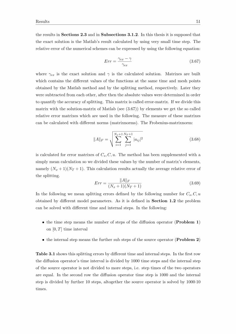
Results 51
the results in Sections 2.3 and in Subsections 3.1.2. In this thesis it is supposed that
the exact solution is the Matlab’s result calculated by using very small time step. The
relative error of the numerical schemes can be expressed by using the following equation:
Err =γex − γγex
(3.67)
where γex is the exact solution and γ is the calculated solution. Matrixes are built
which contains the different values of the functions at the same time and mesh points
obtained by the Matlab method and by the splitting method, respectively. Later they
were subtracted from each other, after then the absolute values were determined in order
to quantify the accuracy of splitting. This matrix is called error-matrix. If we divide this
matrix with the solution-matrix of Matlab (see (3.67)) by elements we get the so called
relative error matrixes which are used in the following. The measure of these matrixes
can be calculated with different norms (matrixnorms). The Frobenius-matrixnorm:
‖A‖F =
√√√√Nx+1∑i=1
NT+1∑j=1
|aij |2 (3.68)
is calculated for error matrixes of Cs, C, u. The method has been supplemented with a
simply mean calculation so we divided these values by the number of matrix’s elements,
namely (Nx + 1)(NT + 1). This calculation results actually the average relative error of
the splitting.
Err =‖A‖F
(Nx + 1)(NT + 1)(3.69)
In the following we mean splitting errors defined by the following number for Cs, C, u
obtained by different model parameters. As it is defined in Section 1.2 the problem
can be solved with different time and internal steps. In the following:
• the time step means the number of steps of the diffusion operator (Problem 1)
on [0, T ] time interval
• the internal step means the further sub steps of the source operator (Problem 2)
Table 3.1 shows this splitting errors by different time and internal steps. In the first row
the diffusion operator’s time interval is divided by 1000 time steps and the internal step
of the source operator is not divided to more steps, i.e. step times of the two operators
are equal. In the second row the diffusion operator time step is 1000 and the internal
step is divided by further 10 steps, altogether the source operator is solved by 1000·10
times.
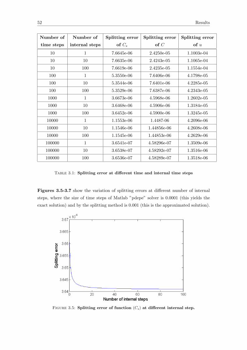
52 Results
Number of Number of Splitting error Splitting error Splitting error
time steps internal steps of Cs of C of u
10 1 7.6645e-06 2.4250e-05 1.1003e-04
10 10 7.6635e-06 2.4243e-05 1.1065e-04
10 100 7.6619e-06 2.4235e-05 1.1554e-04
100 1 5.3550e-06 7.6406e-06 4.1798e-05
100 10 5.3544e-06 7.6401e-06 4.2285e-05
100 100 5.3529e-06 7.6387e-06 4.2343e-05
1000 1 3.6673e-06 4.5968e-06 1.2602e-05
1000 10 3.6468e-06 4.5906e-06 1.3184e-05
1000 100 3.6452e-06 4.5900e-06 1.3245e-05
10000 1 1.1553e-06 1.4487-06 4.2096e-06
10000 10 1.1546e-06 1.44856e-06 4.2608e-06
10000 100 1.1545e-06 1.44853e-06 4.2629e-06
100000 1 3.6541e-07 4.58296e-07 1.3509e-06
100000 10 3.6538e-07 4.58292e-07 1.3516e-06
100000 100 3.6536e-07 4.58289e-07 1.3518e-06
Table 3.1: Splitting error at different time and internal time steps
Figures 3.5-3.7 show the variation of splitting errors at different number of internal
steps, where the size of time steps of Matlab ”pdepe” solver is 0.0001 (this yields the
exact solution) and by the splitting method is 0.001 (this is the approximated solution).
Figure 3.5: Splitting error of function (Cs) at different internal step.
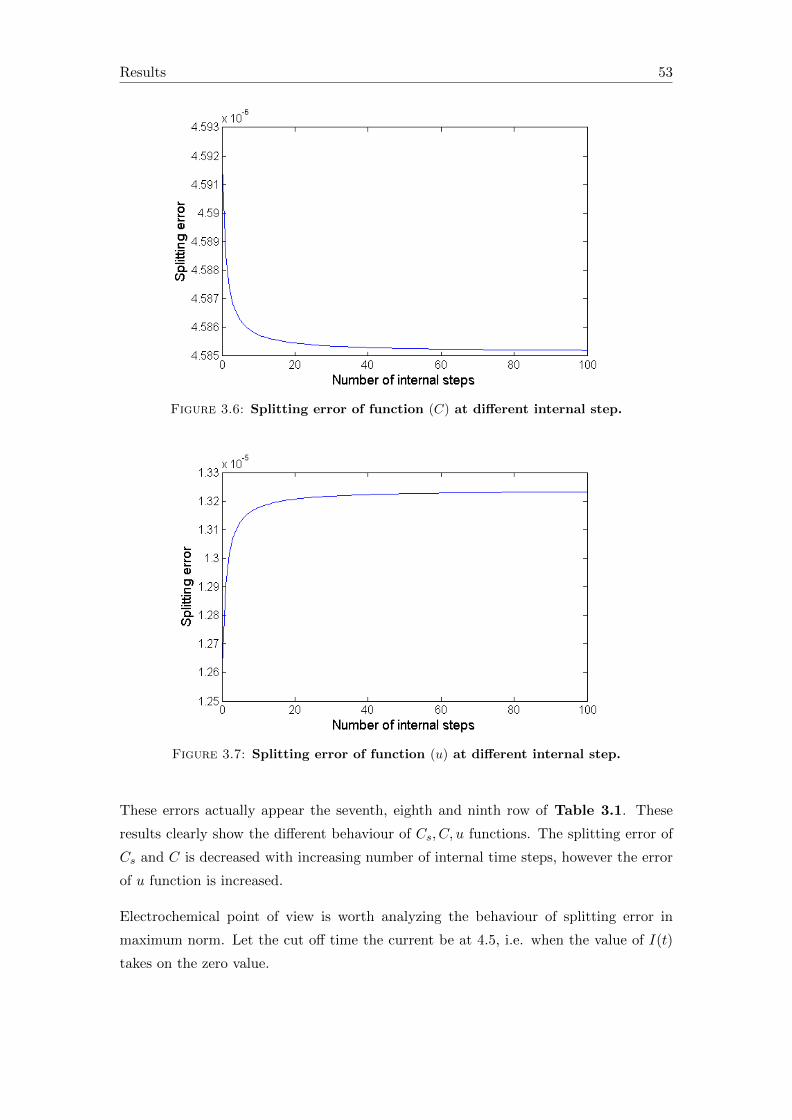
Results 53
Figure 3.6: Splitting error of function (C) at different internal step.
Figure 3.7: Splitting error of function (u) at different internal step.
These errors actually appear the seventh, eighth and ninth row of Table 3.1. These
results clearly show the different behaviour of Cs, C, u functions. The splitting error of
Cs and C is decreased with increasing number of internal time steps, however the error
of u function is increased.
Electrochemical point of view is worth analyzing the behaviour of splitting error in
maximum norm. Let the cut off time the current be at 4.5, i.e. when the value of I(t)
takes on the zero value.
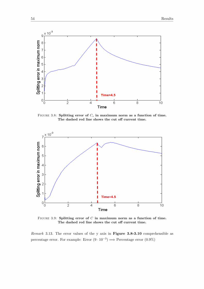
54 Results
Figure 3.8: Splitting error of Cs in maximum norm as a function of time.The dashed red line shows the cut off current time.
Figure 3.9: Splitting error of C in maximum norm as a function of time.The dashed red line shows the cut off current time.
Remark 3.13. The error values of the y axis in Figure 3.8-3.10 comprehensible as
percentage error. For example: Error (9 · 10−3) =⇒ Percentage error (0.9%)
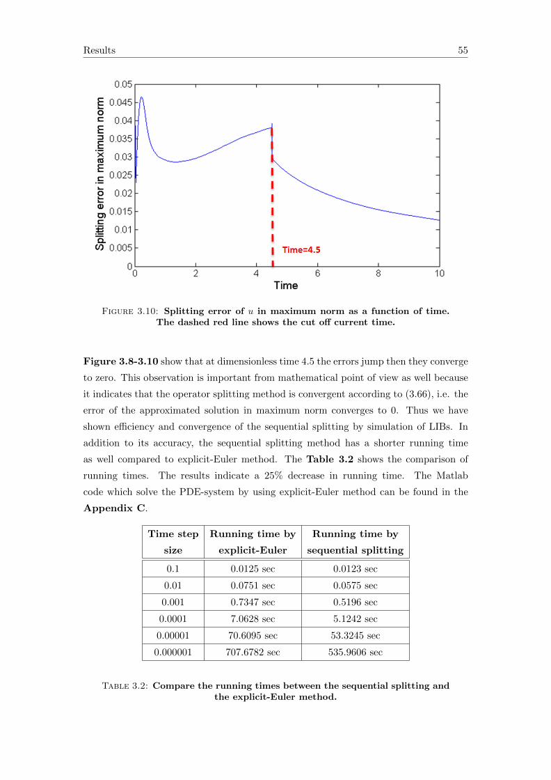
Results 55
Figure 3.10: Splitting error of u in maximum norm as a function of time.The dashed red line shows the cut off current time.
Figure 3.8-3.10 show that at dimensionless time 4.5 the errors jump then they converge
to zero. This observation is important from mathematical point of view as well because
it indicates that the operator splitting method is convergent according to (3.66), i.e. the
error of the approximated solution in maximum norm converges to 0. Thus we have
shown efficiency and convergence of the sequential splitting by simulation of LIBs. In
addition to its accuracy, the sequential splitting method has a shorter running time
as well compared to explicit-Euler method. The Table 3.2 shows the comparison of
running times. The results indicate a 25% decrease in running time. The Matlab
code which solve the PDE-system by using explicit-Euler method can be found in the
Appendix C.
Time step Running time by Running time by
size explicit-Euler sequential splitting
0.1 0.0125 sec 0.0123 sec
0.01 0.0751 sec 0.0575 sec
0.001 0.7347 sec 0.5196 sec
0.0001 7.0628 sec 5.1242 sec
0.00001 70.6095 sec 53.3245 sec
0.000001 707.6782 sec 535.9606 sec
Table 3.2: Compare the running times between the sequential splitting andthe explicit-Euler method.

Chapter 4
Conclusions and outlook
The main aim of this thesis was to investigate the applicability of sequential splitting for
the simulation of LIBs. First, a simplified mathematical model of LIB’s complex system
was derived and was solved by 4 different methods (Matlab’s ”pdepe” solver, sequential
splitting applied for an analytical and a numerical sceme, explicit-Euler method). The
result of Matlab’s ”pdepe” solver was considered to the ”exact” solution, then the other
3 methods were compared with it. In spite of the less complex form of the splitted
operator it was concluded that the analytical solution can be prepared, however its
calculation needs much more resources. More adaptable result was obtained by the
numerical approximation by using the sequential splitting method, which was proven to
be more effective, faster and accurate than the simple explicit-Euler method. We found
furthermore that the application of sequential splitting method for explicit numerical
scheme doesn’t result a sufficiently accurate solution. By replacing the explicit scheme
in the non-linear source term to IMEX scheme we reached a more accurate solution. In
this respect further studies were necessary.
In summary the following can be concluded:
• The sequential splitting method can be applied for the simulation of LIB because
of its small numerical error and its stability over a broad input parameter range.
• The results of the splitting method’s simulation showed a good agreement with
experimental data.
• The developed sequential splitting method needed shorter running time and less
memory than the finite different explicit-Euler method.
• The previous results also imply that the operator splitting methods can be usefully
applied from small scale to large scale (both time and space) for simulation, such
as LIBs.
57
Conclusions and outlook
In the following, we introduce the potential applicability of operator splitting techniques
for the multi-scale modelling of LIB.
Dependency of Cs in the particle domain sub-scale:
A new space variable can be introduced (t > 0)
Cs(x, t) := Cs(r(x), t), x ∈ [0, 1], r(x) ∈ [0, R(x)]
where R(x) is the space dependent radius of the particle. We have to find the solution
of the following PDE at r(x) = R(x)
∂Cs∂t
=1
r2(x)
∂
∂r(x)
(r2(x)D
∂Cs∂r(x)
).
This solution is actually equal to Cs(R(x), t) which yields several local PDE-systems for
all values of x. By this system the boundary conditions are changed in (2.97) according
to the following:
−Dn,p∂Cs∂r(x)
(R(x), t) =J2
an,pF, −Dn,p
∂Cs∂r(x)
(0, t) = 0
In this case the source term and Cs function are actually non-linear PDE-systems, whose
solution is the next step of my work.
For the sake of more realistic simulation it is recommended to apply the original equa-
tions in (1.1)-(1.9).
In Sections 2.1-2.2 was used some of simplifications (Simplifications I.-V.) which
made the calculation significantly easier, however this approach doesn’t take into ac-
count all the electrochemical behaviour of the LIB. In addition to the introduction of
these equations, the applied macrohomogeneous approach shall be extended to the other
two Ω2,Ω3 parts and to other domains such as particle scale.
The result of current work proved that the accuracy can be managed for complex prob-
lems and only splitting does not cause huge error in the system. Therefore operator
splitting can be used as a next generation multi-scale modeling technique to simulate
electrochemical devices including Li-ion batteries in a more sophisticated and precise
way.
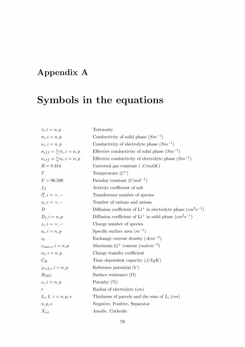
Appendix A
Symbols in the equations
τi, i = n, p Tortuosity
σi, i = n, p Conductivity of solid phase (Sm−1)
κi, i = n, p Conductivity of electrolyte phase (Sm−1)
σeff = εiτiσi, i = n, p Effective conductivity of solid phase (Sm−1)
κeff = εiτiκi, i = n, p Effective conductivity of electrolyte phase (Sm−1)
R = 8.314 Universal gas constant ( J/molK)
T Temperature (C)
F = 96.500 Faraday constant (Cmol−1)
fA Activity coefficient of salt
t0i , i = +,− Transference number of species
νi, i = +,− Number of cations and anions
D Diffusion coefficient of Li+ in electrolyte phase (cm2s−1)
Di, i = n, p Diffusion coefficient of Li+ in solid phase (cm2s−1)
zi, i = +,− Charge number of species
ai, i = n, p Specific surface area (m−1)
i0 Exchange current density (Acm−2)
cmax,i, i = n, p Maximum Li+ content (molcm−3)
αi, i = n, p Charge transfer coefficient
Cdl Time dependent capacity (J/kgK)
ϕref,i, i = n, p Reference potential (V )
RSEI Surface resistance (Ω)
εi, i = n, p Porosity (%)
r Radius of electrolyte (cm)
Li, L i = n, p, s Thickness of parcels and the sum of Li (cm)
n, p, s Negative, Positive, Separator
Xa,c Anodic, Cathodic
59

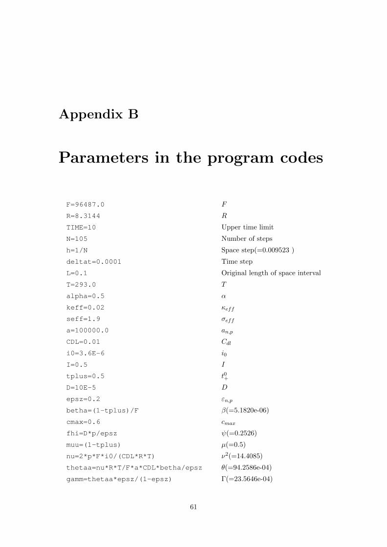
Appendix B
Parameters in the program codes
F=96487.0 F
R=8.3144 R
TIME=10 Upper time limit
N=105 Number of steps
h=1/N Space step(=0.009523 )
deltat=0.0001 Time step
L=0.1 Original length of space interval
T=293.0 T
alpha=0.5 α
keff=0.02 κeff
seff=1.9 σeff
a=100000.0 an,p
CDL=0.01 Cdl
i0=3.6E-6 i0
I=0.5 I
tplus=0.5 t0+
D=10E-5 D
epsz=0.2 εn,p
betha=(1-tplus)/F β(=5.1820e-06)
cmax=0.6 cmax
fhi=D*p/epsz ψ(=0.2526)
muu=(1-tplus) µ(=0.5)
nu=2*p*F*i0/(CDL*R*T) ν2(=14.4085)
thetaa=nu*R*T/F*a*CDL*betha/epsz θ(=94.2586e-04)
gamm=thetaa*epsz/(1-epsz) Γ(=23.5646e-04)
61
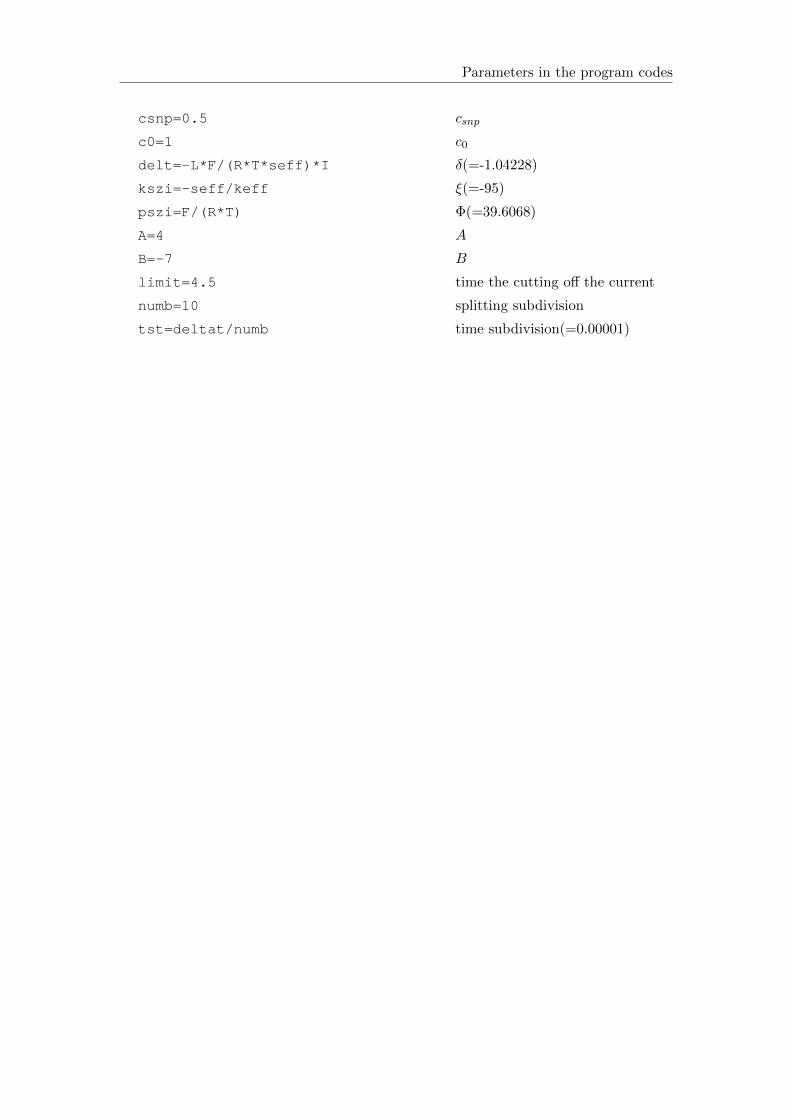
Parameters in the program codes
csnp=0.5 csnp
c0=1 c0
delt=-L*F/(R*T*seff)*I δ(=-1.04228)
kszi=-seff/keff ξ(=-95)
pszi=F/(R*T) Φ(=39.6068)
A=4 A
B=-7 B
limit=4.5 time the cutting off the current
numb=10 splitting subdivision
tst=deltat/numb time subdivision(=0.00001)
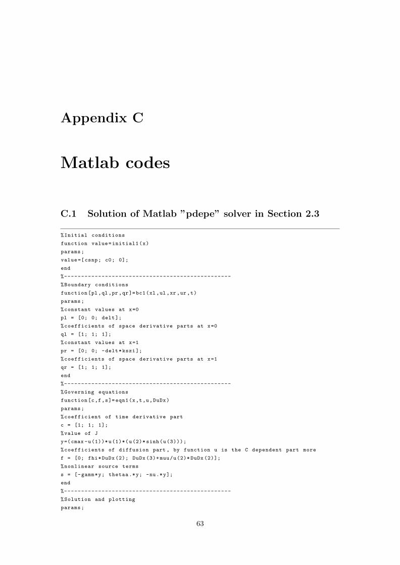
Appendix C
Matlab codes
C.1 Solution of Matlab ”pdepe” solver in Section 2.3
%Initial conditions
function value=initial1(x)
params;
value=[csnp; c0; 0];
end
%-------------------------------------------------
%Boundary conditions
function[pl,ql ,pr,qr]=bc1(xl ,ul,xr,ur ,t)
params;
%constant values at x=0
pl = [0; 0; delt];
%coefficients of space derivative parts at x=0
ql = [1; 1; 1];
%constant values at x=1
pr = [0; 0; -delt*kszi];
%coefficients of space derivative parts at x=1
qr = [1; 1; 1];
end
%-------------------------------------------------
%Governing equations
function[c,f,s]=eqn1(x,t,u,DuDx)
params;
%coefficient of time derivative part
c = [1; 1; 1];
%value of J
y=(cmax -u(1))*u(1)*(u(2)* sinh(u(3)));
%coefficients of diffusion part , by function u is the C dependent part more
f = [0; fhi*DuDx (2); DuDx (3)+ muu/u(2)* DuDx (2)];
%nonlinear source terms
s = [-gamm*y; thetaa .*y; -nu.*y];
end
%-------------------------------------------------
%Solution and plotting
params;
63
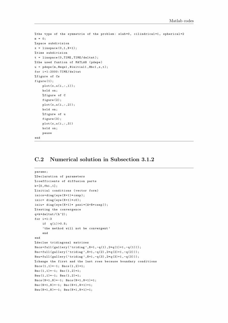
Matlab codes
%the type of the symmetrie of the problem: slab=0, cilindrical =1, spherical =2
m = 0;
%space subdivision
x = linspace (0,1,N+1);
%time subdivision
t = linspace(0,TIME ,TIME/deltat );
%the used funtion of MATLAB (pdepe)
u = pdepe(m,@eqn1 ,@initial1 ,@bc1 ,x,t);
for i=1:2000: TIME/deltat
%figure of Cs
figure (1);
plot(x,u(i,: ,1));
hold on;
%figure of C
figure (2);
plot(x,u(i,: ,2));
hold on;
%figure of u
figure (3);
plot(x,u(i,: ,3))
hold on;
pause
end
C.2 Numerical solution in Subsection 3.1.2
params;
%Declaration of parameters
%coefficients of diffusion parts
k=[0,fhi ,1];
%initial conditions (vector form)
inics=diag(eye(N+1)* csnp);
inic= diag(eye(N+1)*c0);
iniu= diag(eye(N+1)* pszi*(A+B*csnp ));
%testing the convergence
q=k*deltat /(h^2);
for i=1:3
if q(i)>0.5;
’the method will not be convergent ’
end
end
%declae tridiagonal matrixes
Bncs=full(gallery(’tridiag ’,N+1,-q(1) ,2*q(1)+1,-q(1)));
Bnc=full(gallery(’tridiag ’,N+1,-q(2) ,2*q(2)+1,-q(2)));
Bnu=full(gallery(’tridiag ’,N+1,-q(3) ,2*q(3)+1,-q(3)));
%change the first and the last rows because boundary conditions
Bncs (1 ,1)=-1; Bncs (1 ,2)=1;
Bnc (1 ,1)=-1; Bnc (1 ,2)=1;
Bnu (1 ,1)=-1; Bnu (1 ,2)=1;
Bncs(N+1,N)=-1; Bncs(N+1,N+1)=1;
Bnc(N+1,N)=-1; Bnc(N+1,N+1)=1;
Bnu(N+1,N)=-1; Bnu(N+1,N+1)=1;
Matlab codes 65
%the inverse of last matrixes
Z=inv(Bncs); P=inv(Bnc); Q=inv(Bnu);
%fix time step size because deltat will be changed later
H=TIME/deltat;
%declare solutionmatrixes
solutioncs=zeros(N+1,H);
solutionc=zeros(N+1,H);
solutionu=zeros(N+1,H);
solutioncs (:,1)= inics;
solutionc (:,1)= inic;
solutionu (:,1)= iniu;
%declare matrixes for the nonlinear operator
sol4=zeros(N+1,2);
sol5=zeros(N+1,2);
sol6=zeros(N+1,2);
%-------------------------------------------------
%The splitting method
for z=2:H
%declare solution matrixes for the first splitting step
Y=zeros(N+1,2);
W=zeros(N+1,2);
%solution of Cs sin the first step
sol1=inics;
%first array is because the initial condition
Y(: ,1)= inic;
W(: ,1)= iniu;
%declare the f function (Eq (5.53))
U=Y(:,1); U(1)=0; U(N+1)=0;
M=W(:,1);
if deltat <limit
M(1)=h*delt;
M(N+1)=h*delt*kszi;
else
M(1)=0;
M(N+1)=0;
end
%the algorithm for solving the linear equation system
for j=1:N+1
Y(j,2)=P(j,:)*U;
W(j,2)=Q(j,:)*M;
end
%solution of C and u in the first step
sol2=Y(:,2);
sol3=W(:,2);
%the cycle for smaller time steps by nonlinear operator
for l=1: numb
%declare initial conditions
sol4 (: ,1)= sol1;
sol5 (: ,1)= sol2;
sol6 (: ,1)= sol3;
%calculate the different values
sol6 (1 ,2)=( muu *( -1/( sol2 (1))^2+1/ sol2 (1)*( sol2(2)-sol2 (1))/h)
-nu*(cmax -sol1 (1)* sol1 (1)* sol2 (1)* sinh(sol3(1)-pszi*(A+B*sol1 (1))))
*tst+sol6 (1,1);
for i=1:N+1
66 Matlab codes
sol4(i,2)=(- gamm )*(cmax -sol1(i))* sol1(i)*sol2(i)
*sinh(sol3(i)-pszi*(A+B*sol1(i)))* tst+sol4(i,1);
sol5(i,2)=( thetaa )*(cmax -sol1(i))* sol1(i)*sol2(i)
*sinh(sol3(i)-pszi*(A+B*sol1(i)))* tst+sol5(i,1);
end
for i=2:N
sol6(i,2)=( muu *( -1/( sol2(i))^2+1/ sol2(i)
*(sol2(i+1)-2* sol2(i)+sol2(i -1))/h^2)
-nu*(cmax -sol1(i))* sol1(i)*sol2(i)
*sinh(sol3(i)-pszi*(A+B*sol1(i))))* tst+sol6(i,1);
end
sol6(N+1 ,2)=( muu*(-1/( sol2(N+1))^2+1/ sol2(N+1)*( sol2(N+1)-sol2(N))/h)
-nu*(cmax -sol1(N+1))* sol1(N+1)* sol2(N+1)
*sinh(sol3(N+1)-pszi*(A+B*sol1(N+1))))* tst+sol6(N+1,1);
%change the initial conditions
sol1=sol4 (: ,2);
sol2=sol5 (: ,2);
sol3=sol6 (: ,2);
end
%filling the solution matrix
solutioncs (:,z)=sol1;
solutionc(:,z)=sol2;
solutionu(:,z)=sol3;
%change the initial conditions
inics=sol1;
inic=sol2;
iniu=sol3;
deltat=deltat +0.001;
end
%-------------------------------------------------
%Plotting functions
x=linspace (0,1,N+1);
t= linspace(0,TIME ,TIME/deltat );
for i=1:200:H
figure (1);
plot(x,solutioncs (:,i))
hold on;
figure (2)
plot(x,solutionc(:,i))
hold on;
figure (3);
plot(x,solutionu(:,i))
hold on;
pause
end
C.3 Explicit-Euler’s method in Subsection 3.2
for z=2:H
for i=1:N+1
sol1(i)=(-gamm )*(cmax -inics(i))* inics(i)*inic(i)
*sinh(iniu(i)-pszi*(A+B*inics(i)))+ inics(i);
Matlab codes 67
end
Y=zeros(N+1,2);
Y(: ,1)= inic;
U=Y(:,1); U(1)=0; U(N+1)=0;
for i=1:N+1
Y(i,2)=P(i,:)*U-S*(-thetaa )*(cmax -inics(i))* inics(i)*inic(i)
*sinh(iniu(i)-pszi*(A+B*inics(i)));
end
sol2=Y(:,2);
W=zeros(N+1,2);
W(: ,1)= iniu;
M=W(:,1);
if deltat <limit
M(1)=h*delt; M(N+1)=h*delt*kszi;
else
M(1)=0; M(N+1)=0;
end
W(1 ,2)=Q(1,:)*M-S*(muu*(-1/( inic (1))^2+1/ inic (1)*( inic(2)-inic (1))/h)
-nu*(cmax -inics (1))* inics (1)* inic (1)* sinh(iniu(1)-pszi*(A+B*inics (1))));
for i=2:N
W(i,2)=Q(i,:)*M-S*(muu*(-1/( inic(i))^2+1/ inic(i)*
(inic(i+1) -2* inic(i)+inic(i-1))/h^2)-nu*(cmax -inics(i))* inics(i)*inic(i)
*sinh(iniu(i)-pszi*(A+B*inics(i))));
end
W(N+1,2)=Q(N+1,:)*M-S*(muu*(-1/( inic(N+1))^2+1/ inic(N+1)
*(inic(N+1)-inic(N))/h)-nu*(cmax -inics(N+1))* inics(N+1)* inic(N+1)
*sinh(iniu(N+1)-pszi*(A+B*inics(N+1))));
sol3=W(:,2);
solutioncs (:,z)=sol1;
solutionc(:,z)=sol2;
solutionu(:,z)=sol3;
inics=sol1;
inic=sol2;
iniu=sol3;
deltat=deltat +0.001;
end

Bibliography[1] Bombay Harbor (2015); http://www.bombayharbor.com/productImage/0184564001238654414/
Battery Ion Battery Pack Lithium Battery Lithium Ion.jpg
[2] Physics and Society (2015); https://physicsandsocietybc.files.wordpress.com/
2013/04/meriampic.gif
[3] V. Ramadesigan, P. W. C. Northrop, S. De, S. Santhanagopalan, R.
D. Braatz, V. R. Subramanian; Modeling and Simulation of Lithium-Ion Batteries
from a Systems Engineering Perspective; Journal of The Electrochemical Society, 159
(3), 2012
[4] Alejandro A. Franco; Multiscale modelling and numerical simulation of recharge-
able lithium ion batteries: concepts, methods and challenges; The Royal Society of Chem-
istry 2013, Pages 13027−13058
[5] Christopher Taylor; Integrated multiscale modelling of materials; DNV GL Strate-
gic Research & Innovation Position Paper 8, 2014, Pages 4−20
[6] Rene de Borst; Challenges in computational materials science: Multiple scales,
multi-physics and evolving discontinuities; Comp. Mater. Sci. 43, 2008, Pages 1−15
[7] A. Havasi, J. Bartholy, I. Farago; Splitting method and its application in air
pollution modelling; Idojrs ISSN 0324-6329 CODEN IDOJA4, 2001, Pages 39−58
[8] M.A. Botchev, I. Farago, R. Horvath; Application of operator splitting to the
Maxwell equations including a source term; Applied Numerical Mathematics 59, 2009,
Pages 522−541
[9] A. Kriston, Gy. Inzelt, I. Farago, T. Szabo; Simulation of the transient
behaviour of fuel cells by using operator splitting techniques for real-time applications;
Computers and Chemical Engineering 34, 2008, Pages 339−348
[10] John Newman, Karen E. Thomas-Alyea; Electrochemical Systems Third Edi-
tion, Copyright by John Wiley & Sons, Inc., Hoboken, New Jersey, 2004
69
Bibliography
[11] U. M. Ascher, S. J. Ruuth, and B. T. R. Wetton; Implicit-explicit methods
for time-dependent partial differential equations; SIAM J. Numer. Anal. 32(3), 1995,
Pages 797−823
[12] Farago Istvan, Horvath Robert; Numerikus modszerek, Masodik, javıtott kiadas;
Copyright by Farago Istvan, ELTE, Horvath Robert, BME, Budapest, 2013
[13] Istvan Farago; A modified iterated operator splitting method; Applied Mathemat-
ical Modelling, 2008, Pages 1542−1551
[14] G.-H. Kim, K. Smith, K.-J. Lee, S. Santhanagopalan, A. Pesaran; Multi-
Domain Modeling of Lithium-Ion Batteries Encompassing Multi-Physics in Varied Length
Scales; The Electrochemical Society 158(8), 2011, Pages 955−969
[15] M. Gomadam, J. W. Weidner, R. A. Dougal, R. E. White; Mathematical
modeling of lithium-ion and nickel battery systems; Journal of Power Sources 110; 2002
Pages 267−284
[16] R. D. Skeel, M. Bezins; A method for the spatial discretization of parabolic
equations in one space variable; SIAM J. Sci. and Stat. Comput. 11(1), 1990, Pages
1−32
[17] Roger A. Horn and Charles R. Johnson; Matrix Analysis; Copyright by Cam-
bridge University, 1990, Pages 357−363
[18] P. Csomos, I. Farago, A. Havasi; Weighted Sequential Splittings and Their
Analysis; Computers & Mathematics with Applications 50(7), 2005, Pages 1017−1031
[19] I. Farago, J. Geiser; Iterative operator-splitting methods for linear problems;
International Mathematical Forum 6, 2011, 2737−2770