3D photography

Kevin Köser, Marc Pollefeys

Spring 2012

http://www.cvg.ethz.ch/teaching/2012spring/3dphoto/

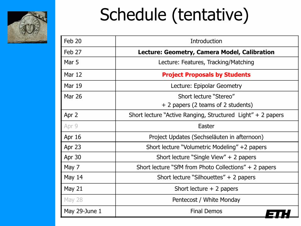
Feb 20 Introduction

Feb 27 Lecture: Geometry, Camera Model, Calibration

Mar 5 Lecture: Features, Tracking/Matching

Mar 12 Project Proposals by Students

Mar 19 Lecture: Epipolar Geometry

Mar 26 Short lecture “Stereo”

+ 2 papers (2 teams of 2 students)

Apr 2 Short lecture “Active Ranging, Structured Light” + 2 papers

Apr 9 Easter

Apr 16 Project Updates (Sechseläuten in afternoon)

Apr 23 Short lecture “Volumetric Modeling” +2 papers

Apr 30 Short lecture “Single View” + 2 papers

May 7 Short lecture “SfM from Photo Collections” + 2 papers

May 14 Short lecture “Silhouettes” + 2 papers

May 21 Short lecture + 2 papers

May 28 Pentecost / White Monday

May 29-June 1 Final Demos

Schedule (tentative)

Projective Geometry and Camera model

Class 2

points, lines, planes conics and quadrics

transformations camera model

See http://www.cs.unc.edu/~marc/tutorial/

Book: Hartley/Zisserman: “Multiple View Geometry in Computer Vision”

Homogeneous coordinates

0=++ cbyax ( ) ( ) 0=1x,y,a,b,cT

( ) ( ) 0≠∀,~ ka,b,cka,b,cTT

Homogeneous representation of 2D points and lines

equivalence class of vectors, any vector is representative

Set of all equivalence classes in R3(0,0,0)T forms P2

( ) ( ) 0≠∀,1,,~1,, kyxkyxTT

The point x lies on the line l if and only if

Homogeneous coordinates

Inhomogeneous coordinates ( )Tyx,

( )T321 ,, xxx but only 2DOF

Note that scale is unimportant for incidence relation

0=xlT

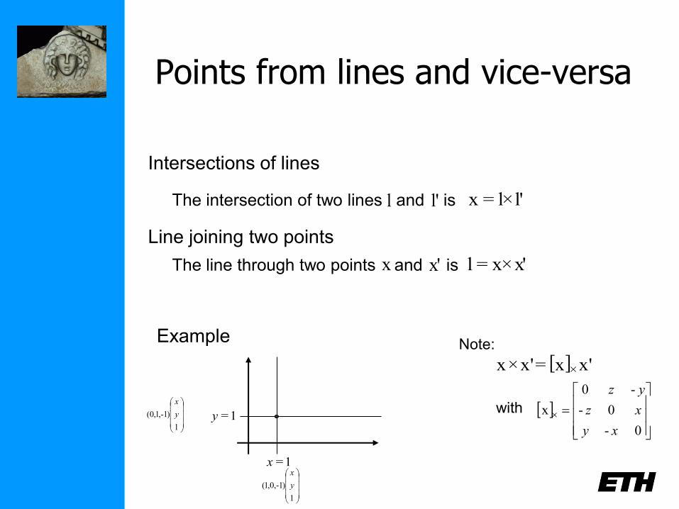
Points from lines and vice-versa

l'×l=x

Intersections of lines

The intersection of two lines and is l l'

Line joining two points

The line through two points and is x'×x=lx x'

Example

1=x

1=y

1

)1-,1,0( y

x

1

)1-,0,1( y

x

Note:

[ ] 'xx='x×x ×

with

0-

0-

-0

x

xy

xz

yz

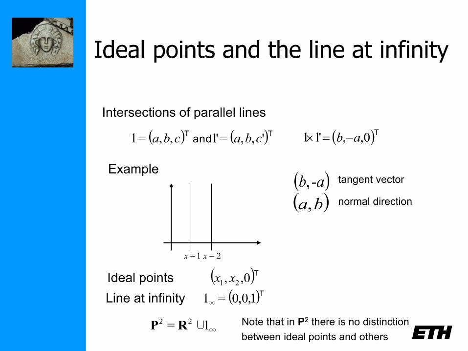
Ideal points and the line at infinity

T0,,l'l ab

Intersections of parallel lines

( ) ( )TTand ',,=l' ,,=l cbacba

Example

1=x 2=x

Ideal points ( )T0,, 21 xx

Line at infinity ( )T1,0,0=l∞

∞22 l∪= RP

tangent vector

normal direction

-ab,

( )ba,

Note that in P2 there is no distinction

between ideal points and others

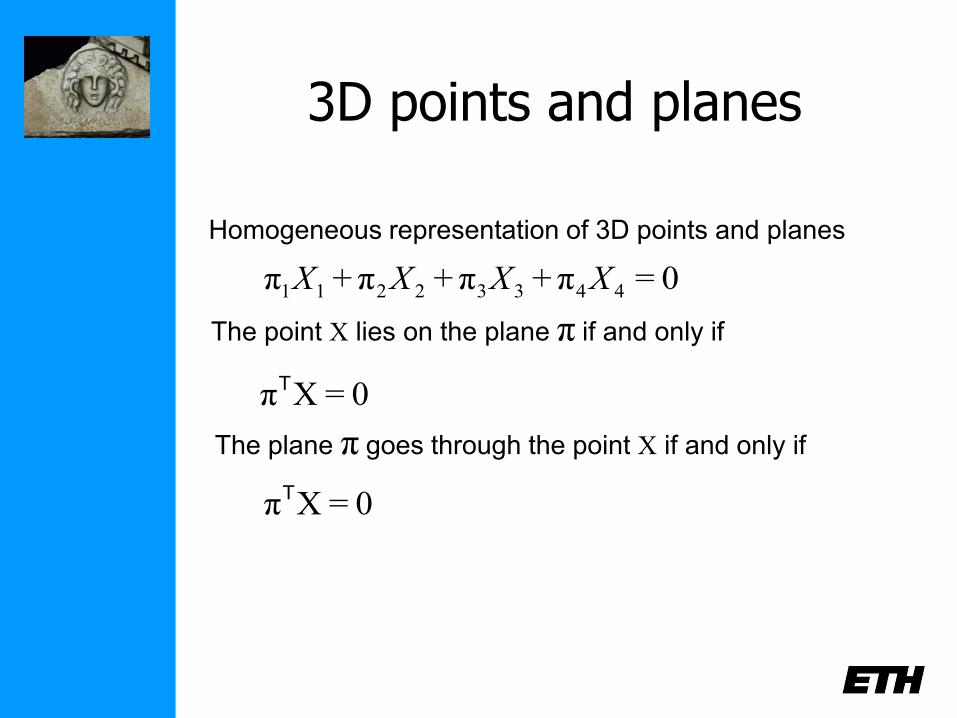
3D points and planes

Homogeneous representation of 3D points and planes

The point X lies on the plane π if and only if

0=π+π+π+π 44332211 XXXX

0=XπT

The plane π goes through the point X if and only if

0=XπT

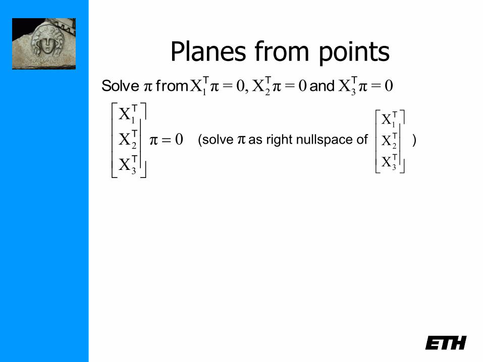
Planes from points

0π

X

X

X

3

2

1

T

T

T

0=πX 0=πX 0,=πX π 321

TTTandfromSolve

(solve as right nullspace of ) π

T

T

T

3

2

1

X

X

X

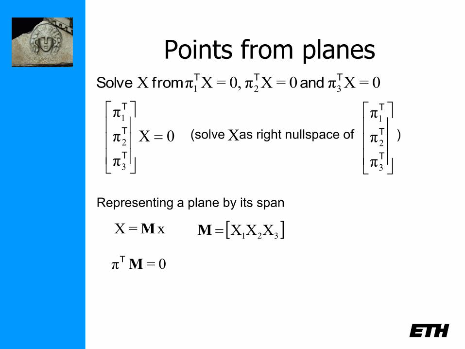
Points from planes

0X

π

π

π

3

2

1

T

T

T

x=X M 321 XXXM

0=π MT

0=Xπ 0=Xπ 0,=Xπ X 321

TTTandfromSolve

(solve as right nullspace of ) X

T

T

T

3

2

1

π

π

π

Representing a plane by its span

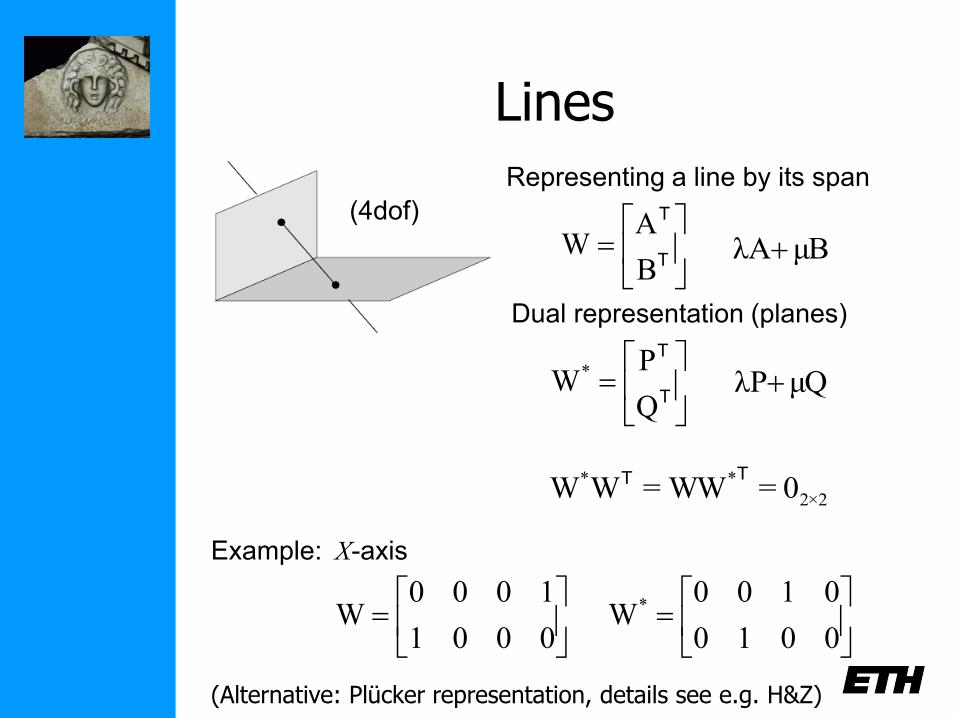
Lines

T

T

B

AW μBλA

2×2

** 0=WW=WWTT

0001

1000W

0010

0100W*

Example: X-axis

(4dof)

Representing a line by its span

T

T

Q

PW*

μQλP

Dual representation (planes)

(Alternative: Plücker representation, details see e.g. H&Z)

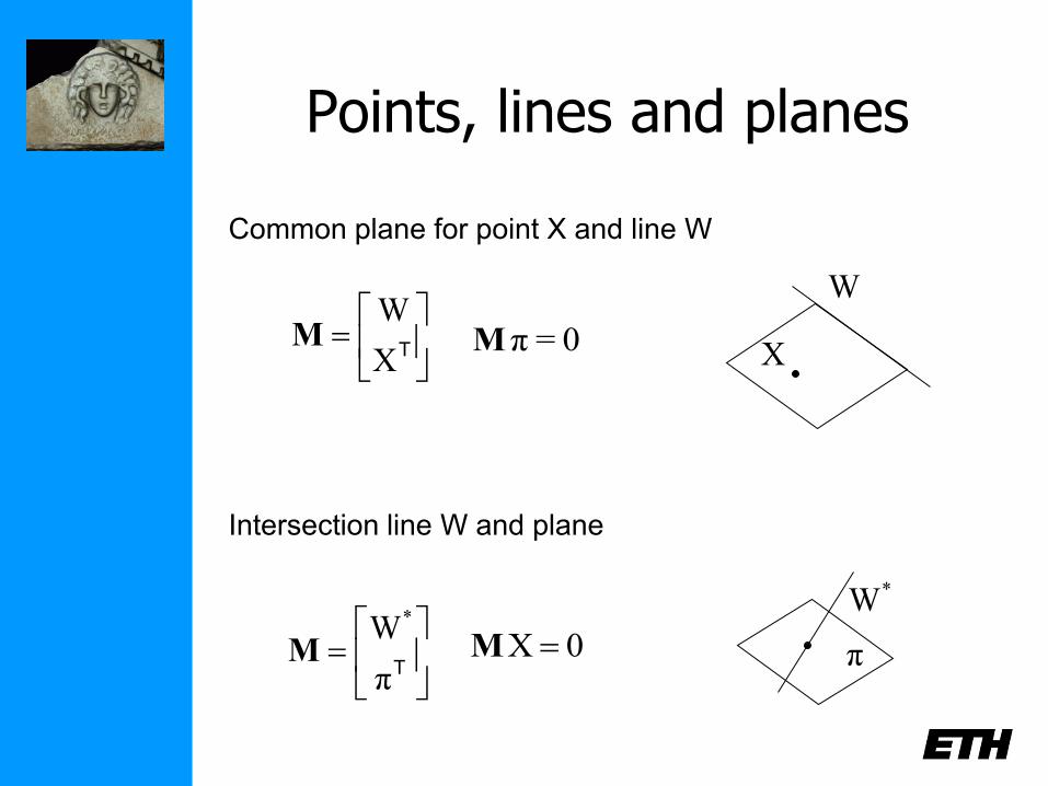
Points, lines and planes

TX

WM 0=πM

Tπ

W*

M 0X M

W

X

*W

π

Common plane for point X and line W

Intersection line W and plane

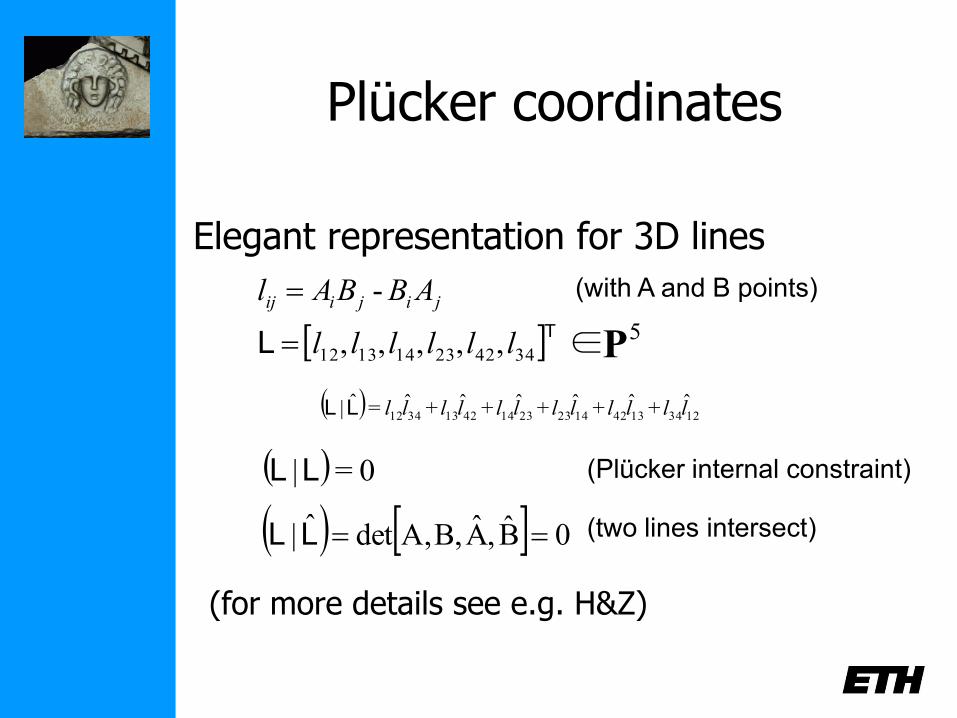
Plücker coordinates

Elegant representation for 3D lines

jijiij ABBAl -

TL 344223141312 ,,,,, llllll 5∈P

0B,AB,A,detˆ| LL

( ) 0=|LL (Plücker internal constraint)

(two lines intersect)

( )123413421423231442133412ˆ+ˆ+ˆ+ˆ+ˆ+ˆ=ˆ| llllllllllllLL

(for more details see e.g. H&Z)

(with A and B points)

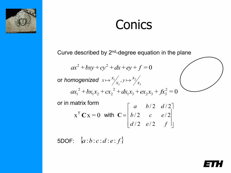
Conics

Curve described by 2nd-degree equation in the plane

0=+++++ 22 feydxcybxyax

0=+++++ 2

33231

2

221

2

1 fxxexxdxcxxbxax

3

2

3

1 ,x

xy

xx

x or homogenized

0=xx CT

or in matrix form

fed

ecb

dba

2/2/

2/2/

2/2/

Cwith

{ }fedcba :::::5DOF:

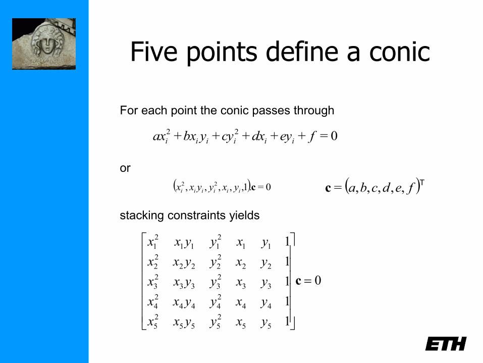
Five points define a conic

For each point the conic passes through

0=+++++ 22 feydxcyybxax iiiiii

or

( ) 0=.1,,,,, 22ciiiiii yxyyxx ( )T

fedcba ,,,,,=c

0

1

1

1

1

1

55

2

555

2

5

44

2

444

2

4

33

2

333

2

3

22

2

222

2

2

11

2

111

2

1

c

yxyyxx

yxyyxx

yxyyxx

yxyyxx

yxyyxx

stacking constraints yields

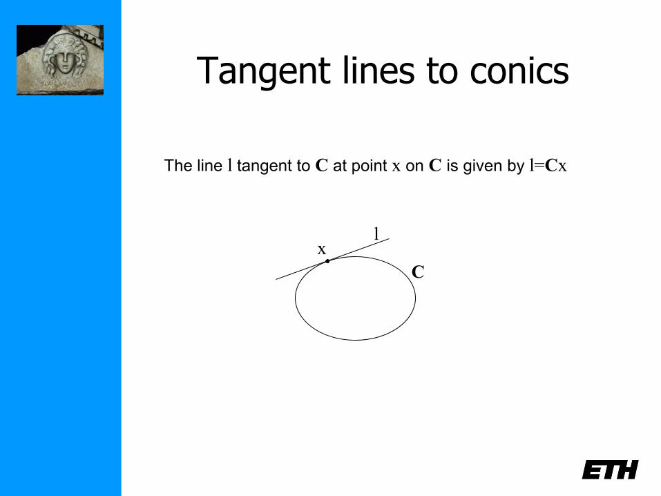
Tangent lines to conics

The line l tangent to C at point x on C is given by l=Cx

l x

C

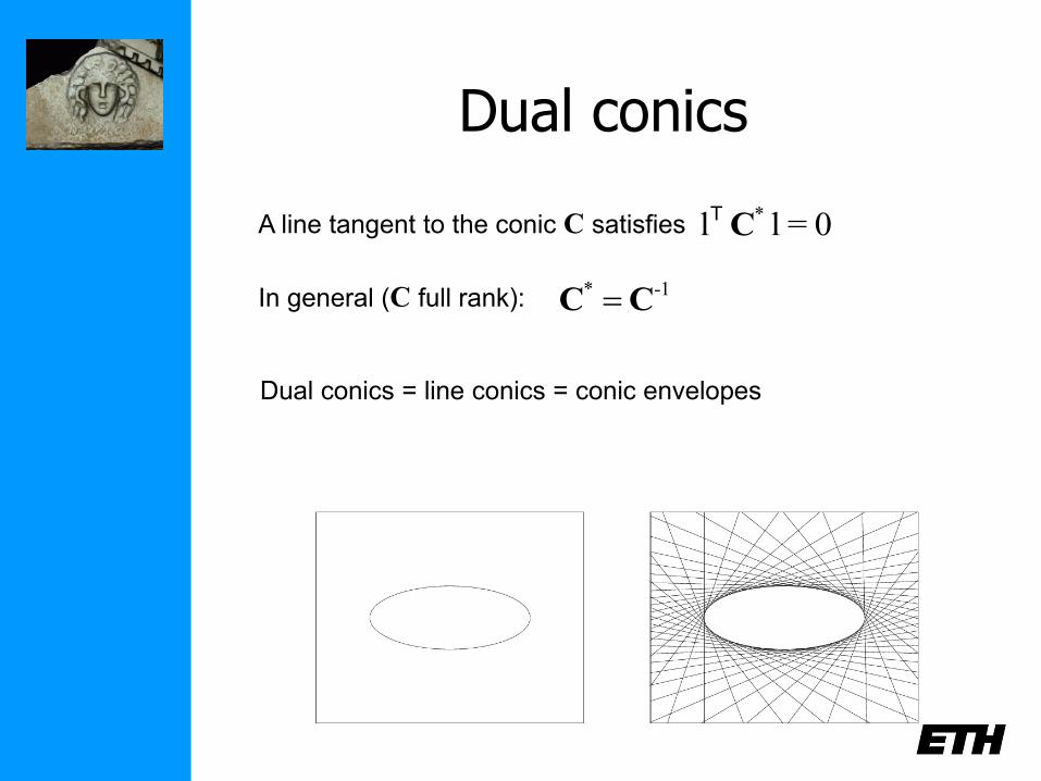
Dual conics

0=ll *C

TA line tangent to the conic C satisfies

Dual conics = line conics = conic envelopes

1-* CC In general (C full rank):

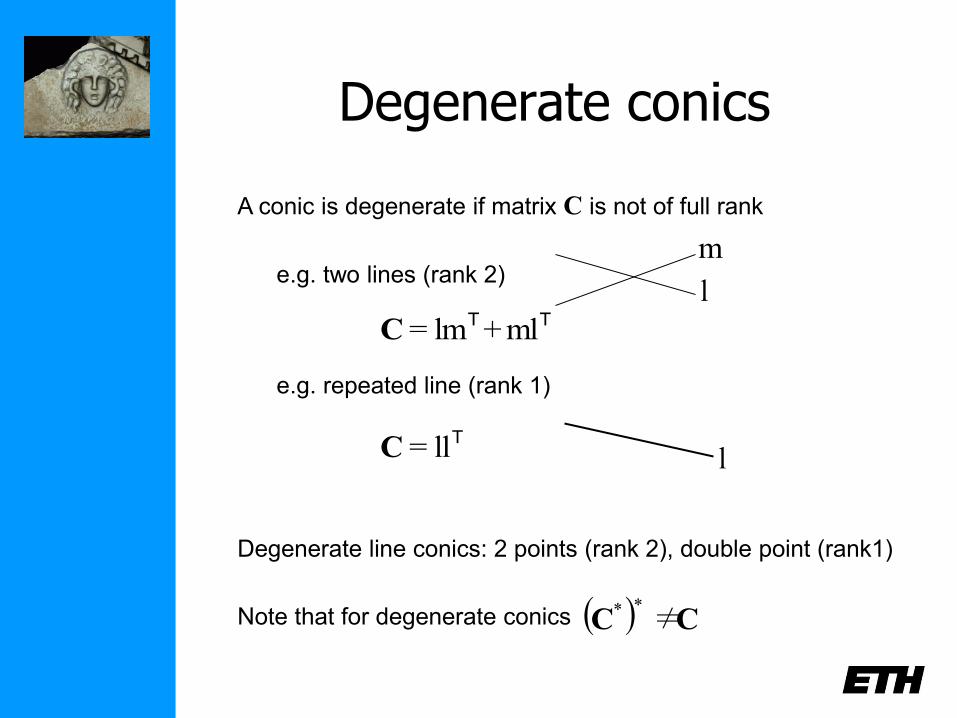
Degenerate conics

A conic is degenerate if matrix C is not of full rank

TT ml+lm=C

e.g. two lines (rank 2)

e.g. repeated line (rank 1)

Tll=C

l

l

m

Degenerate line conics: 2 points (rank 2), double point (rank1)

( ) CC ≠**Note that for degenerate conics

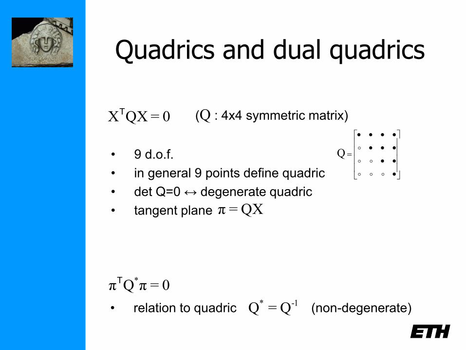
Quadrics and dual quadrics

(Q : 4x4 symmetric matrix) 0=QXXT

• 9 d.o.f.

• in general 9 points define quadric

• det Q=0 ↔ degenerate quadric

• tangent plane

Q

QX=π

0=πQπ *T

-1* Q=Q• relation to quadric (non-degenerate)

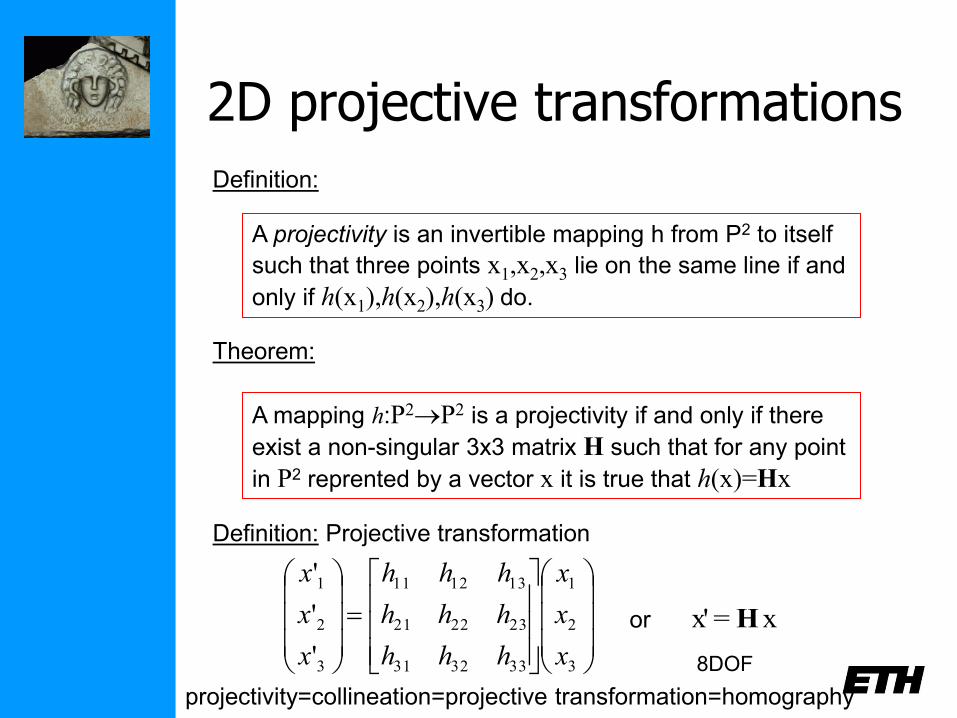
2D projective transformations

A projectivity is an invertible mapping h from P2 to itself

such that three points x1,x2,x3 lie on the same line if and

only if h(x1),h(x2),h(x3) do.

Definition:

A mapping h:P2P2 is a projectivity if and only if there

exist a non-singular 3x3 matrix H such that for any point

in P2 reprented by a vector x it is true that h(x)=Hx

Theorem:

Definition: Projective transformation

3

2

1

333231

232221

131211

3

2

1

'

'

'

x

x

x

hhh

hhh

hhh

x

x

x

x=x' Hor

8DOF

projectivity=collineation=projective transformation=homography

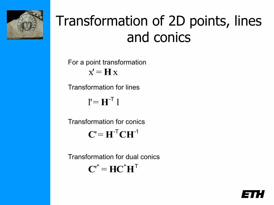
Transformation of 2D points, lines and conics

Transformation for lines

l=l' -TH

Transformation for conics

-1-TCHHC ='

Transformation for dual conics

THHCC

** ='

x=x' HFor a point transformation

Fixed points and lines

e=e λH

(eigenvectors H =fixed points)

l=l λTH

(eigenvectors H-T =fixed lines)

(1=2 pointwise fixed line)

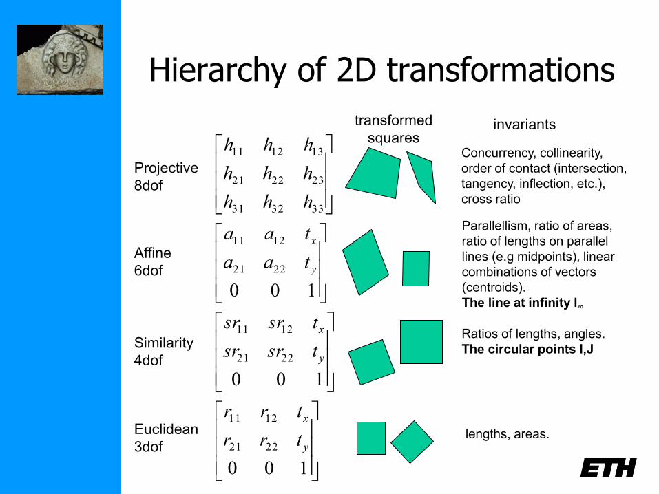
Hierarchy of 2D transformations

100

2221

1211

y

x

taa

taa

100

2221

1211

y

x

tsrsr

tsrsr

333231

232221

131211

hhh

hhh

hhh

100

2221

1211

y

x

trr

trr

Projective

8dof

Affine

6dof

Similarity

4dof

Euclidean

3dof

Concurrency, collinearity,

order of contact (intersection,

tangency, inflection, etc.),

cross ratio

Parallellism, ratio of areas,

ratio of lengths on parallel

lines (e.g midpoints), linear

combinations of vectors

(centroids).

The line at infinity l∞

Ratios of lengths, angles.

The circular points I,J

lengths, areas.

invariants transformed

squares

The line at infinity

3

2

1

1

-

1t-

0ll

l

l

l

AA

AH

T-T

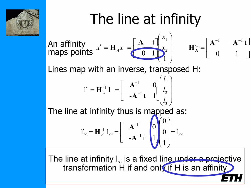
The line at infinity l is a fixed line under a projective transformation H if and only if H is an affinity

110

t2

1

x

x

xx A

AH

10

t11

1- AAHA

An affinity maps points

Lines map with an inverse, transposed H:

∞1∞-

∞ l

1

0

0

1t-

0ll

A

AH

T-T

A

The line at infinity thus is mapped as:

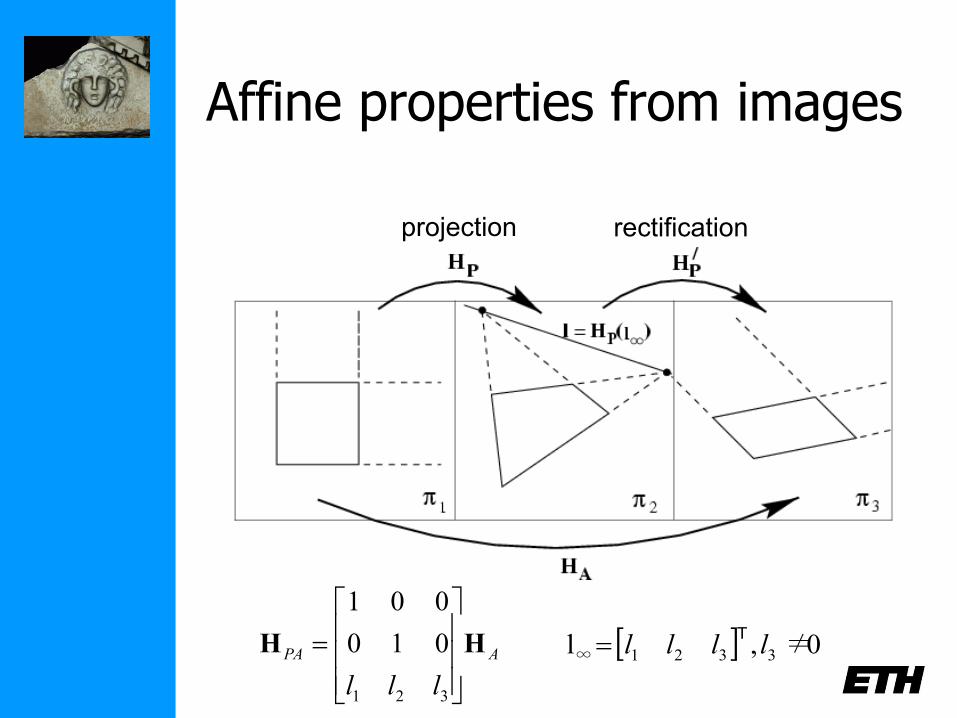
Affine properties from images

projection rectification

APA

lll

HH

321

010

001

0≠,l 3321∞ llllT

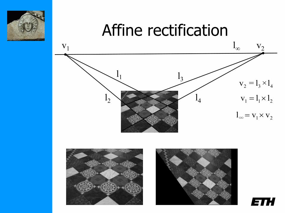
Affine rectification v1 v2

l1

l2 l4

l3

l∞

21∞ vvl

211 llv

432 l×l=v

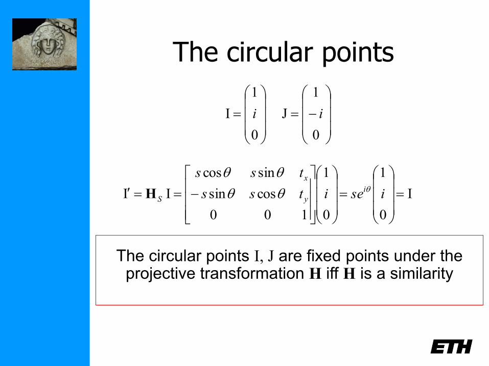
The circular points

0

1

I i

0

1

J i

I

0

1

0

1

100

cossin

sincos

II

iseitss

tssi

y

x

S

H

The circular points I, J are fixed points under the projective transformation H iff H is a similarity

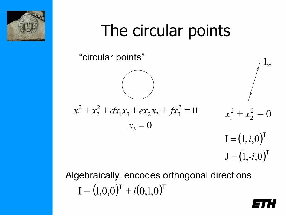
The circular points

“circular points”

0=++++ 2

33231

2

2

2

1 fxxexxdxxx 0=+ 2

2

2

1 xx

l∞

T

T

0,-,1J

0,,1I

i

i

( ) ( )TT0,1,0+0,0,1=I i

Algebraically, encodes orthogonal directions

03 x

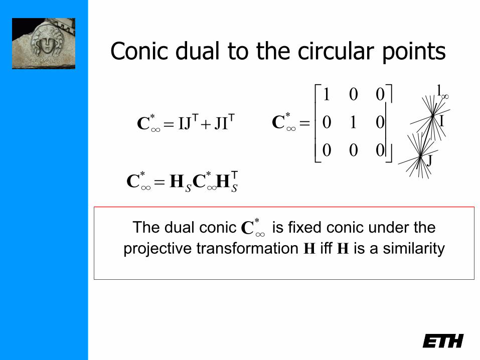
Conic dual to the circular points

TT JIIJ*

∞ C

000

010

001*

∞C

T

SS HCHC*

∞*

∞

The dual conic is fixed conic under the

projective transformation H iff H is a similarity

*

∞C

l∞

I

J

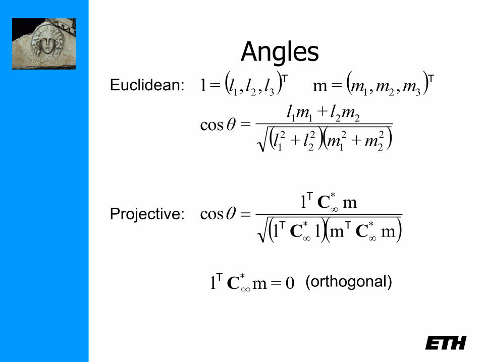
Angles

( )( )2

2

2

1

2

2

2

1

2211

++

+=cos

mmll

mlmlθ

( )T321 ,,=l lll ( )T

321 ,,=m mmm

Euclidean:

Projective: mmll

mlcos

**

*

CC

C

TT

T

0=ml *

∞CT

(orthogonal)

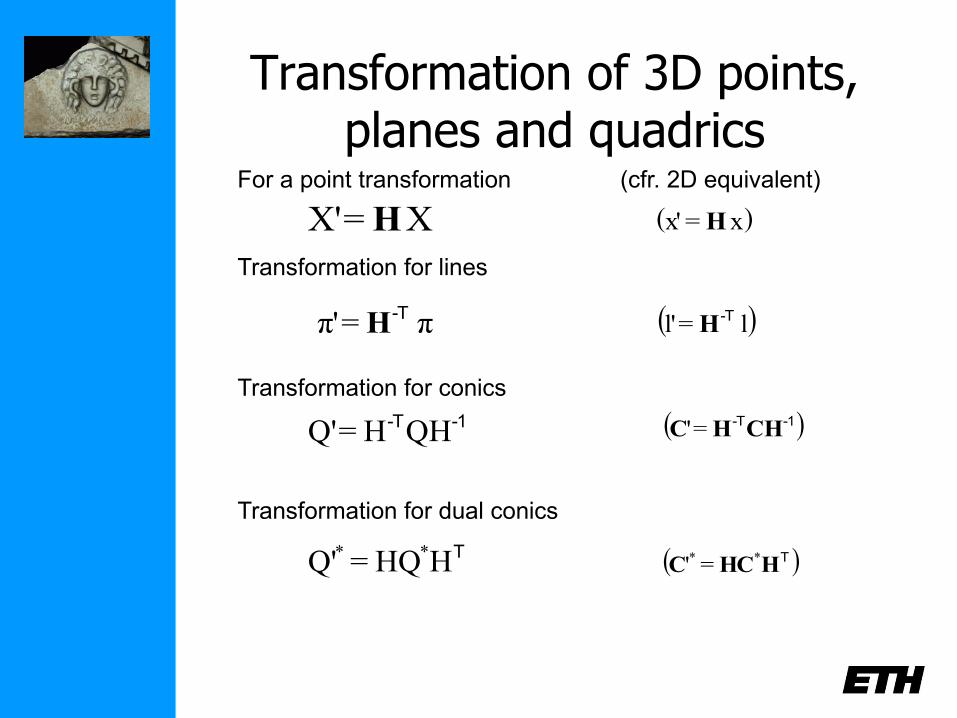
Transformation of 3D points, planes and quadrics

Transformation for lines

( )l=l' -TH

Transformation for conics

( )-1-TCHHC ='

Transformation for dual conics

( )THHCC

** ='

( )x=x' H

For a point transformation

X=X' H

π=π' -TH

-1-TQHH=Q'

THHQ=Q' **

(cfr. 2D equivalent)

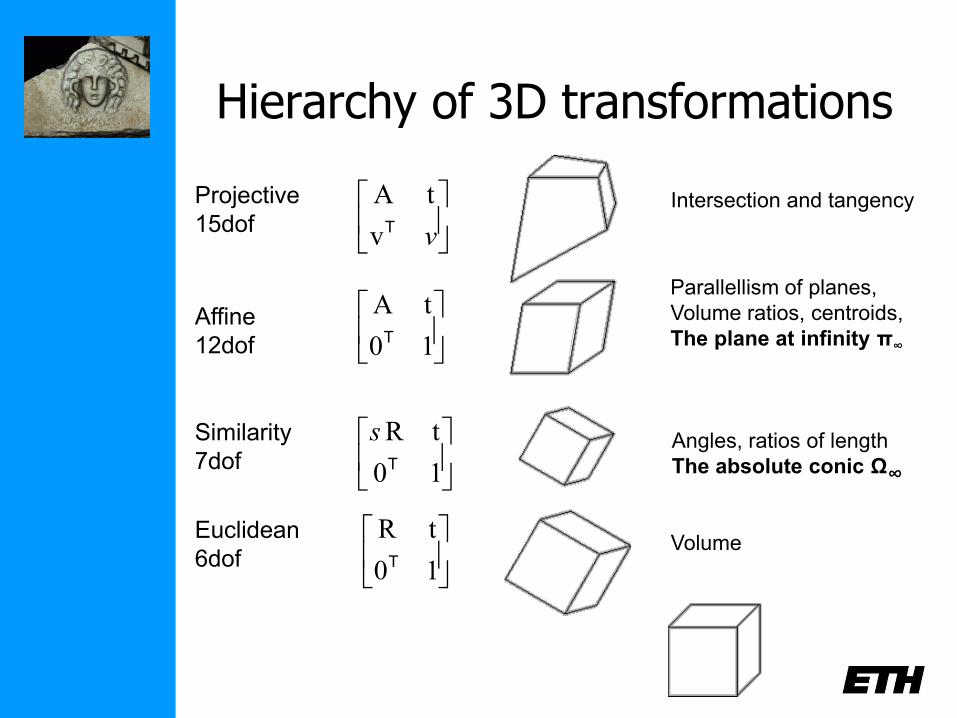
Hierarchy of 3D transformations

vTv

tAProjective

15dof

Affine

12dof

Similarity

7dof

Euclidean

6dof

Intersection and tangency

Parallellism of planes,

Volume ratios, centroids,

The plane at infinity π∞

Angles, ratios of length

The absolute conic Ω∞

Volume

10

tAT

10

tRT

s

10

tRT

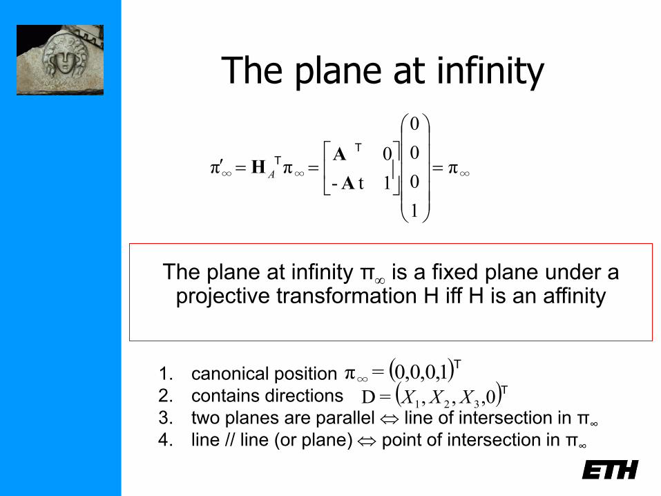
The plane at infinity

∞∞∞ π

1

0

0

0

1t-

0ππ

A

AH

TT

A

The plane at infinity π is a fixed plane under a projective transformation H iff H is an affinity

1. canonical position

2. contains directions

3. two planes are parallel line of intersection in π∞

4. line // line (or plane) point of intersection in π∞

( )T1,0,0,0=π∞

( )T0,,,=D 321 XXX

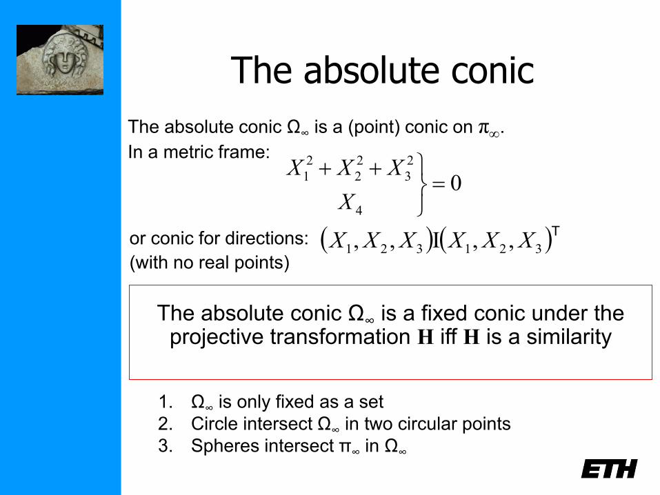
The absolute conic

The absolute conic Ω∞ is a fixed conic under the projective transformation H iff H is a similarity

04

2

3

2

2

2

1

X

XXX

The absolute conic Ω∞ is a (point) conic on π.

In a metric frame:

T321321 ,,I,, XXXXXXor conic for directions:

(with no real points)

1. Ω∞ is only fixed as a set

2. Circle intersect Ω∞ in two circular points

3. Spheres intersect π∞ in Ω∞

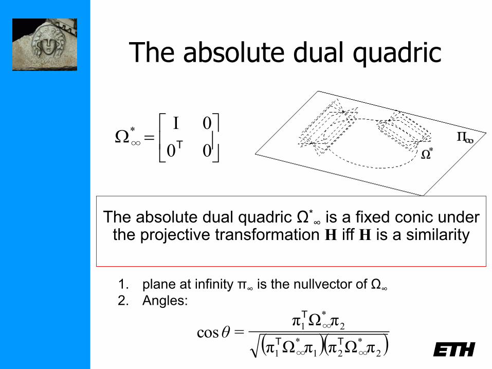
The absolute dual quadric

00

0I*

∞ T

The absolute dual quadric Ω*∞ is a fixed conic under

the projective transformation H iff H is a similarity

1. plane at infinity π∞ is the nullvector of Ω∞

2. Angles:

( )( )2

*

∞21

*

∞1

2

*

∞1

πΩππΩπ

πΩπ=cos

TT

T

θ

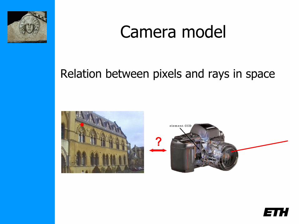
Camera model

Relation between pixels and rays in space

?

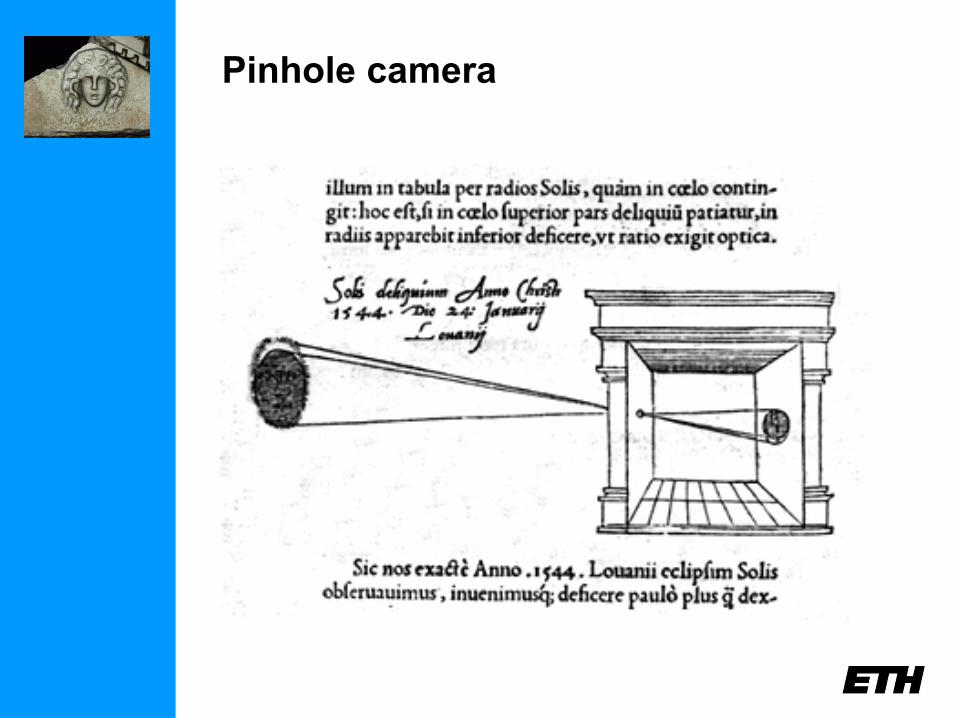
Pinhole camera

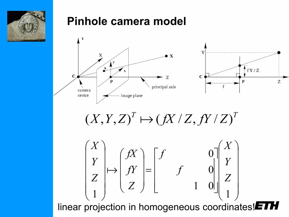
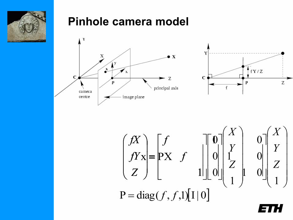
Pinhole camera model

TT ZfYZfXZYX )/,/(),,(

101

0

0

1

Z

Y

X

f

f

Z

fY

fX

Z

Y

X

linear projection in homogeneous coordinates!

Pinhole camera model

101

0

0

Z

Y

X

f

f

Z

fY

fX

101

01

01

1Z

Y

X

f

f

Z

fY

fX

PXx

0|I)1,,(diagP ff

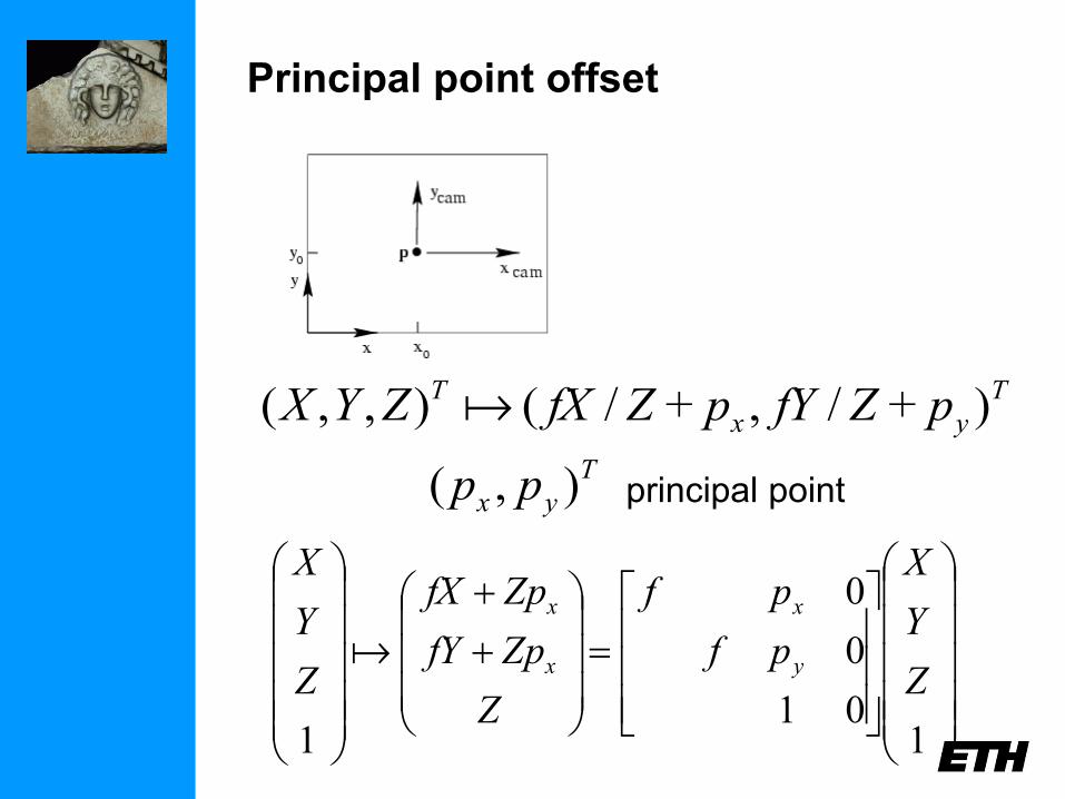
Principal point offset

T

yx

T pZfYpZfXZYX )+/,+/(),,(

principal point T

yx pp ),(

101

0

0

1

Z

Y

X

pf

pf

Z

ZpfY

ZpfX

Z

Y

X

y

x

x

x

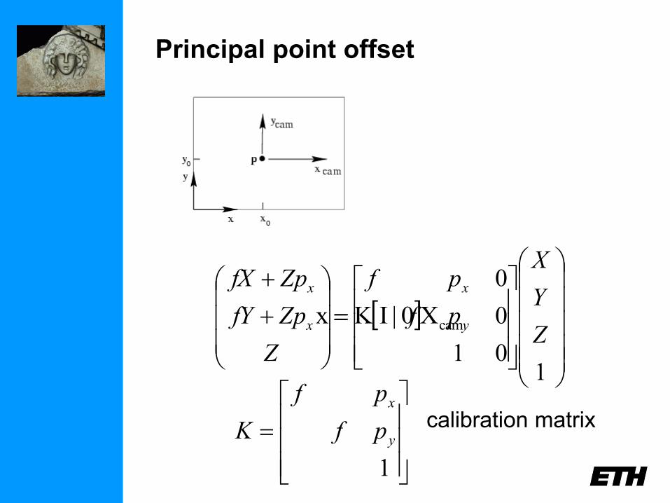
Principal point offset

101

0

0

Z

Y

X

pf

pf

Z

ZpfY

ZpfX

y

x

x

x

camX0|IKx

1

y

x

pf

pf

K calibration matrix

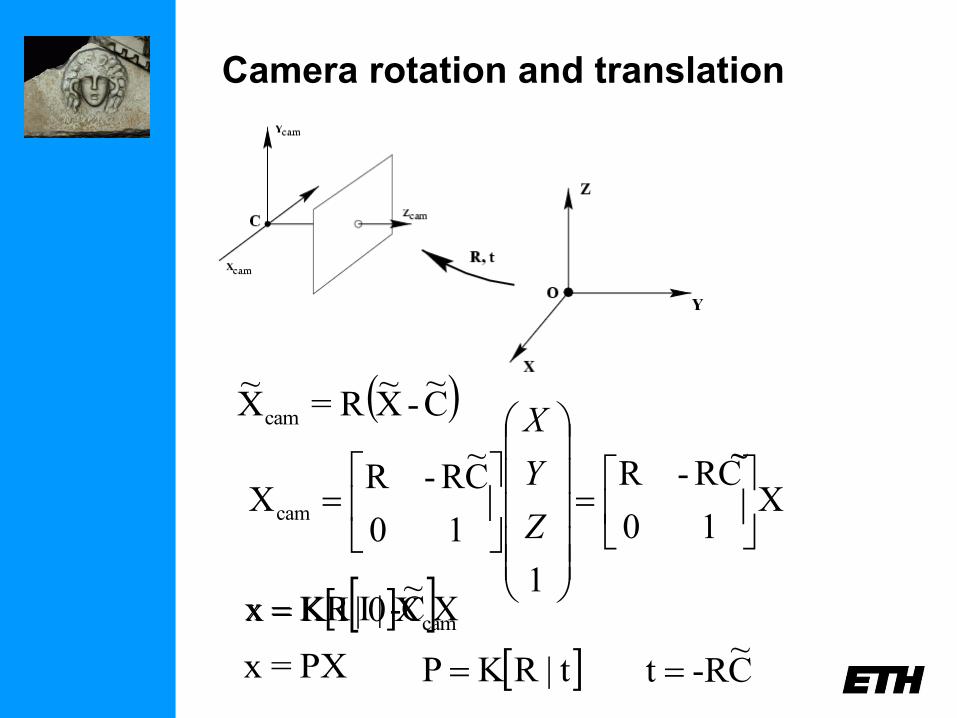
Camera rotation and translation

( )C~

-X~

R=X~

cam

X10

RC-R

1

10

C~

R-RXcam

Z

Y

X

camX0|IKx XC~

-|IKRx

t|RKP C~

R-t PX=x

~

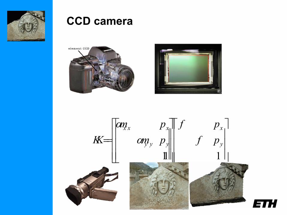
CCD camera

1

yy

xx

p

p

K

11

y

x

y

x

pf

pf

m

m

K

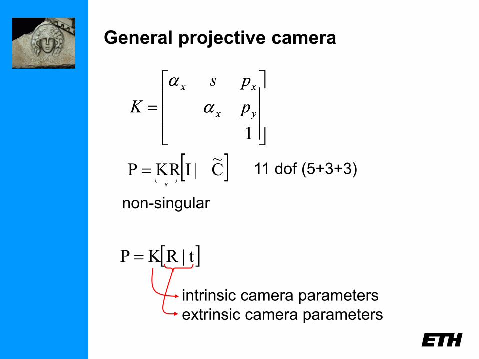
General projective camera

1

yx

xx

p

ps

K

1

yx

xx

p

p

K

C~

|IKRP

non-singular

11 dof (5+3+3)

t|RKP

intrinsic camera parameters

extrinsic camera parameters

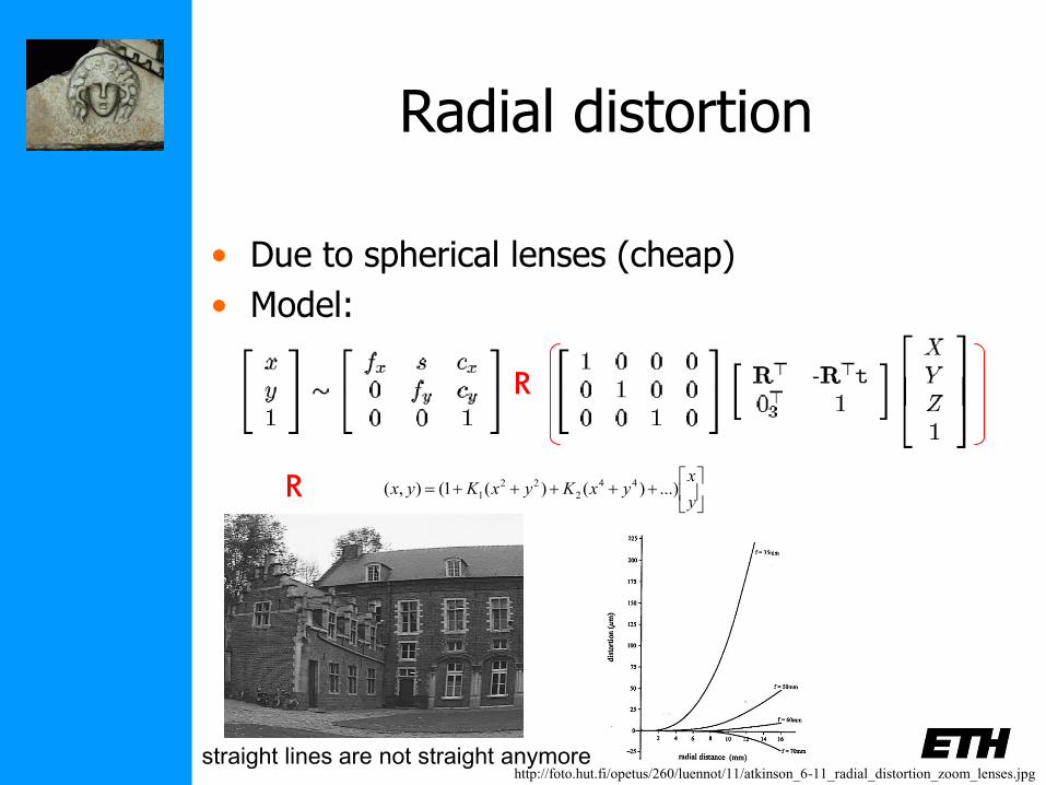
Radial distortion

• Due to spherical lenses (cheap)

• Model:

R

y

xyxKyxKyx ...))()(1(),( 44

2

22

1R

http://foto.hut.fi/opetus/260/luennot/11/atkinson_6-11_radial_distortion_zoom_lenses.jpg straight lines are not straight anymore

Camera model

Relation between pixels and rays in space

?

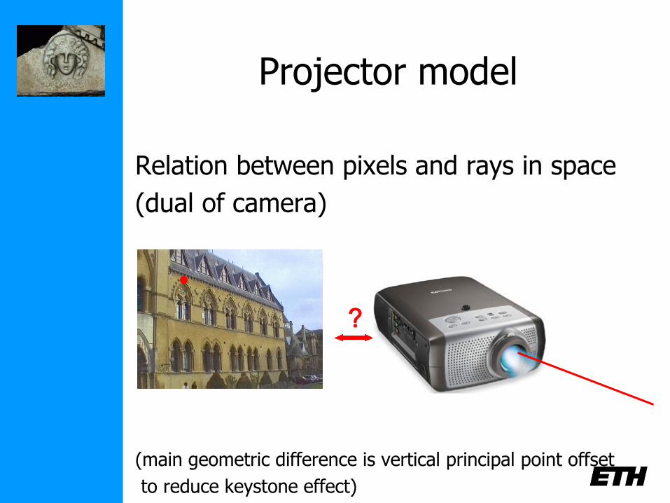
Projector model

Relation between pixels and rays in space

(dual of camera)

(main geometric difference is vertical principal point offset

to reduce keystone effect)

?

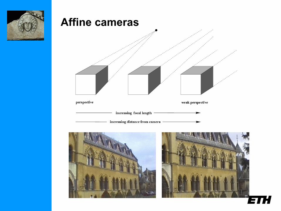
Affine cameras

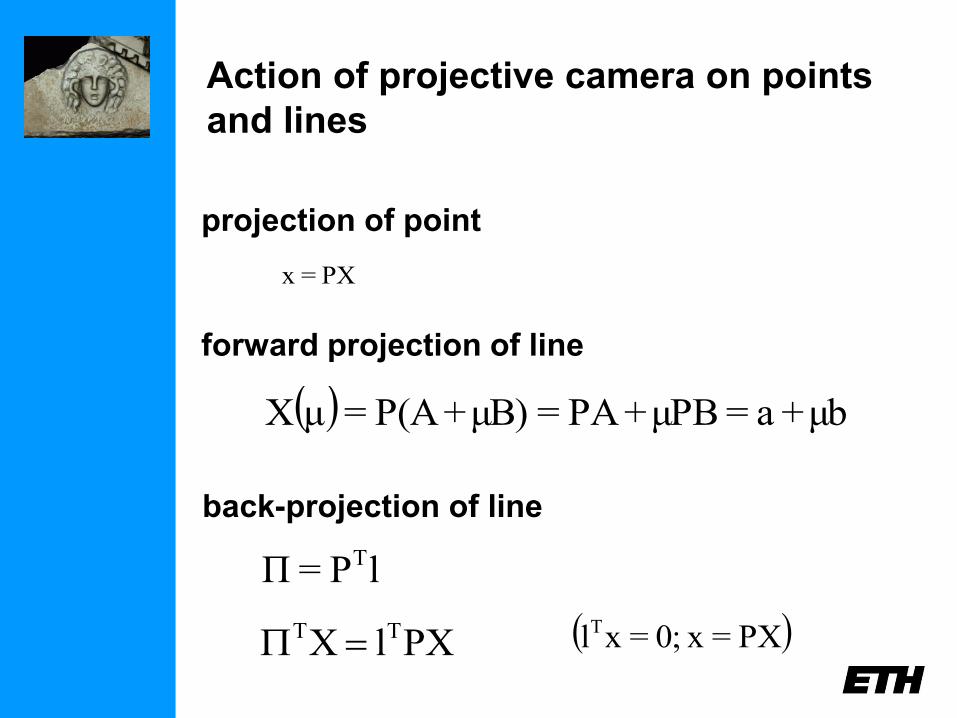
Action of projective camera on points

and lines

forward projection of line

( ) μb+a=μPB+PA=μB)+P(A=μX

back-projection of line

lP=Π T

PXlX TT ( )PX= x0;=xlT

PX=x

projection of point

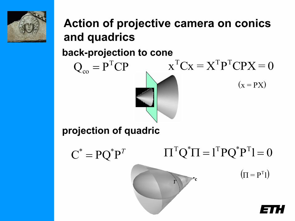
Action of projective camera on conics

and quadrics

back-projection to cone

CPPQ T

co 0=CPXPX=Cxx TTT

( )PX=x

projection of quadric

TPPQC ** 0lPPQlQ T*T*T

( )lP=Π T

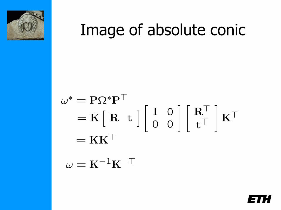
Image of absolute conic

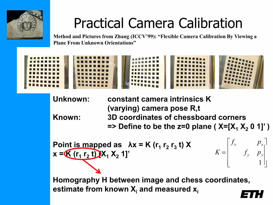
Practical Camera Calibration

Unknown: constant camera intrinsics K

(varying) camera pose R,t

Known: 3D coordinates of chessboard corners

=> Define to be the z=0 plane ( X=[X1 X2 0 1]’ )

Point is mapped as λx = K (r1 r2 r3 t) X

x = K (r1 r2 t) [X1 X2 1]’

1

yy

xx

pf

pf

K

Homography H between image and chess coordinates,

estimate from known Xi and measured xi

Method and Pictures from Zhang (ICCV’99): “Flexible Camera Calibration By Viewing a

Plane From Unknown Orientations”

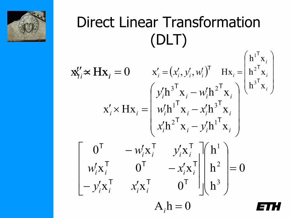
Direct Linear Transformation (DLT)

ii Hxx 0Hxx ii

i

i

i

i

xh

xh

xh

Hx3

2

1

T

T

T

iiii

iiii

iiii

ii

yx

xw

wy

xhxh

xhxh

xhxh

Hxx12

31

23

TT

TT

TT

0

h

h

h

0xx

x0x

xx0

3

2

1

TTT

TTT

TTT

iiii

iiii

iiii

xy

xw

yw

Tiiii wyx ,,x

0hA i

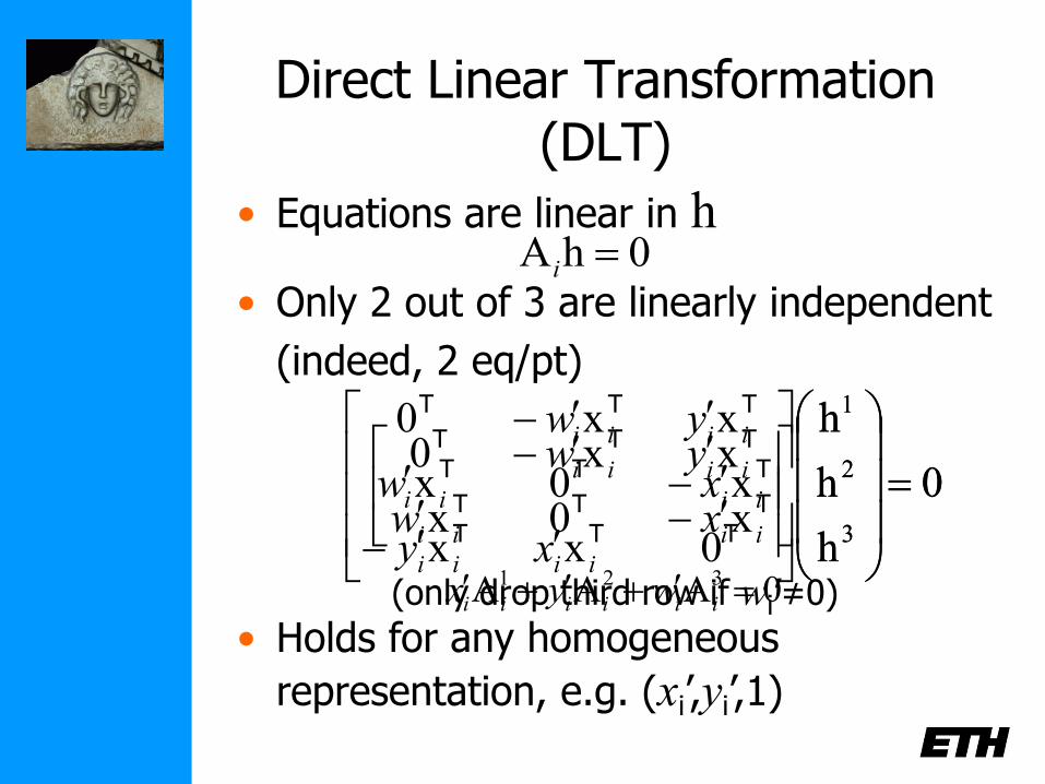
Direct Linear Transformation (DLT)

• Equations are linear in h

0

h

h

h

0xx

x0x

xx0

3

2

1

TTT

TTT

TTT

iiii

iiii

iiii

xy

xw

yw

0AAA 321 iiiiii wyx

0hA i

• Only 2 out of 3 are linearly independent

(indeed, 2 eq/pt)

0

h

h

h

x0x

xx0

3

2

1

TTT

TTT

iiii

iiii

xw

yw

(only drop third row if wi’≠0)

• Holds for any homogeneous

representation, e.g. (xi’,yi’,1)

Direct Linear Transformation (DLT)

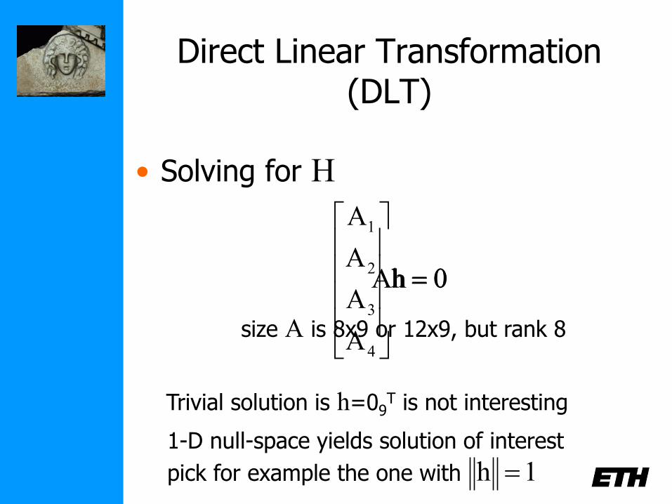
• Solving for H

0Ah 0h

A

A

A

A

4

3

2

1

size A is 8x9 or 12x9, but rank 8

Trivial solution is h=09T is not interesting

1-D null-space yields solution of interest

pick for example the one with 1h

Direct Linear Transformation (DLT)

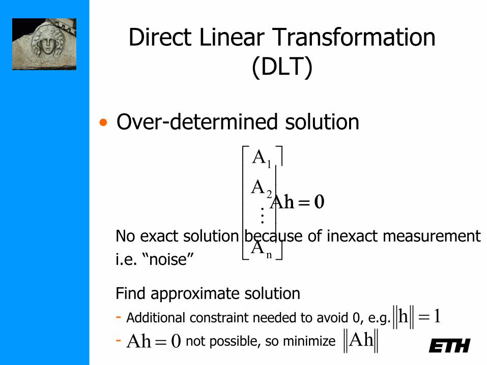
• Over-determined solution

No exact solution because of inexact measurement

i.e. “noise”

0Ah 0h

A

A

A

n

2

1

Find approximate solution

- Additional constraint needed to avoid 0, e.g.

- not possible, so minimize

1h

Ah0Ah

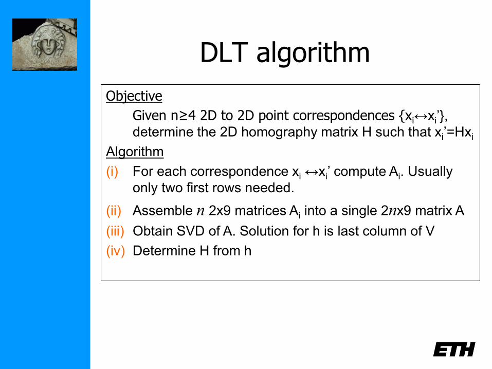
DLT algorithm

Objective

Given n≥4 2D to 2D point correspondences {xi↔xi’},

determine the 2D homography matrix H such that xi’=Hxi

Algorithm

(i) For each correspondence xi ↔xi’ compute Ai. Usually

only two first rows needed.

(ii) Assemble n 2x9 matrices Ai into a single 2nx9 matrix A

(iii) Obtain SVD of A. Solution for h is last column of V

(iv) Determine H from h

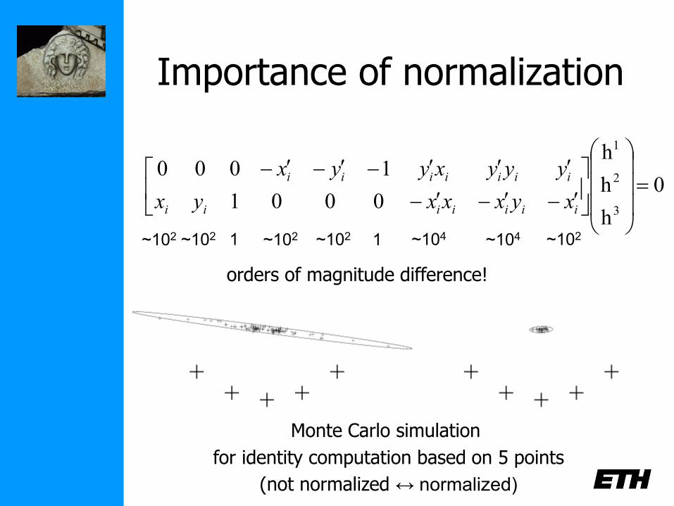
Importance of normalization

0

h

h

h

0001

1000

3

2

1

iiiiiii

iiiiiii

xyxxxyx

yyyxyyx

~102 ~102 ~102 ~102 ~104 ~104 ~102 1 1

orders of magnitude difference!

Monte Carlo simulation

for identity computation based on 5 points

(not normalized ↔ normalized)

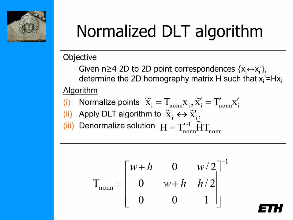
Normalized DLT algorithm

Objective

Given n≥4 2D to 2D point correspondences {xi↔xi’},

determine the 2D homography matrix H such that xi’=Hxi

Algorithm

(i) Normalize points

(ii) Apply DLT algorithm to

(iii) Denormalize solution

,x~x~ ii

inormiinormi xTx~,xTx~

norm

-1

norm TH~

TH

1

norm

100

2/0

2/0

T

hhw

whw

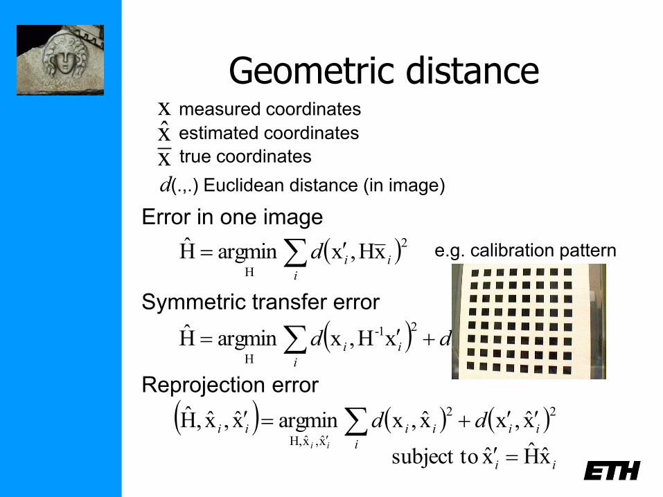
Geometric distance measured coordinates

estimated coordinates

true coordinates

xxx

2H

xH,xargminH ii

i

d

Error in one image

e.g. calibration pattern

221-

H

Hx,xxH,xargminH iiii

i

dd

Symmetric transfer error

d(.,.) Euclidean distance (in image)

ii

iiii

i

ii ddii

xHx subject to

x,xx,xargminx,x,H22

x,xH,

Reprojection error

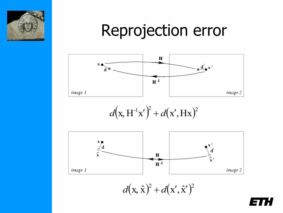
Reprojection error

221- Hx,xxHx, dd

22x,xxx, dd

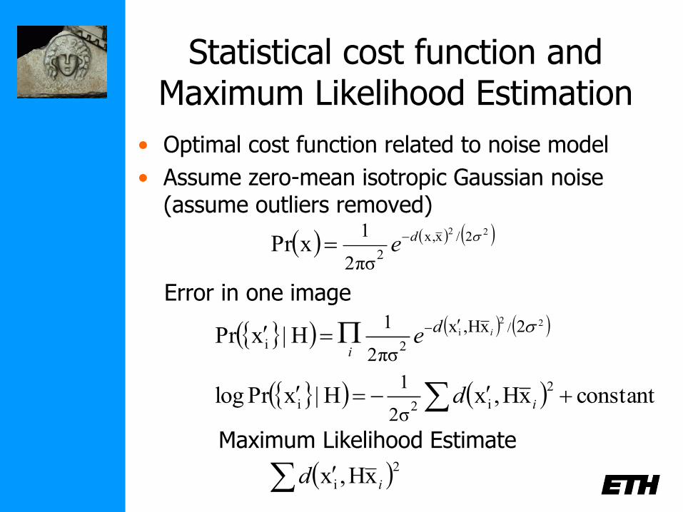
Statistical cost function and Maximum Likelihood Estimation

• Optimal cost function related to noise model

• Assume zero-mean isotropic Gaussian noise (assume outliers removed)

22

2/xx,

2πσ2

1xPr de

22

i 2xH,x /

2iπσ2

1H|xPr

ide

i

constantxH,xH|xPrlog2

i2iσ2

1id

Error in one image

Maximum Likelihood Estimate

2

i xH,x id

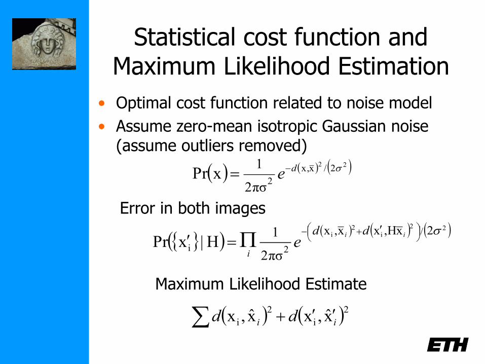
Statistical cost function and Maximum Likelihood Estimation

• Optimal cost function related to noise model

• Assume zero-mean isotropic Gaussian noise (assume outliers removed)

22

2/xx,

2πσ2

1xPr de

22

i2

i 2xH,xx,x /

2iπσ2

1H|xPr

ii dd

ei

Error in both images

Maximum Likelihood Estimate

2i

2

i x,xx,x ii dd

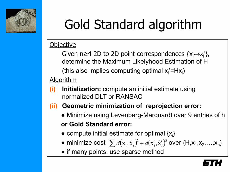
Gold Standard algorithm

Objective

Given n≥4 2D to 2D point correspondences {xi↔xi’},

determine the Maximum Likelyhood Estimation of H

(this also implies computing optimal xi’=Hxi)

Algorithm

(i) Initialization: compute an initial estimate using

normalized DLT or RANSAC

(ii) Geometric minimization of reprojection error:

● Minimize using Levenberg-Marquardt over 9 entries of h

or Gold Standard error:

● compute initial estimate for optimal {xi}

● minimize cost over {H,x1,x2,…,xn}

● if many points, use sparse method

2i

2

i x,xx,x ii dd

Practical Camera Calibration

Unknown: constant camera intrinsics K

(varying) camera pose R,t

Known: 3D coordinates of chessboard corners

=> Define to be the z=0 plane ( X=[X1 X2 0 1]’ )

Point is mapped as λx = K (r1 r2 r3 t) X

x = K (r1 r2 t) [X1 X2 1]’

1

yy

xx

pf

pf

K

Homography H between image and chess coordinates,

estimate from known Xi and measured xi

Method and Pictures from Zhang (ICCV’99): “Flexible Camera Calibration By Viewing a

Plane From Unknown Orientations”

Practical Camera Calibration

1

yy

xx

pf

pf

K

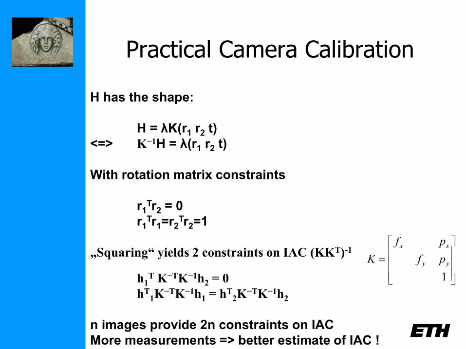
H has the shape:

H = λK(r1 r2 t)

<=> K−1H = λ(r1 r2 t)

With rotation matrix constraints

r1Tr2 = 0

r1Tr1=r2

Tr2=1

„Squaring“ yields 2 constraints on IAC (KKT)-1

h1T K−TK−1h2 = 0

hT1K

−TK−1h1 = hT2K

−TK−1h2

n images provide 2n constraints on IAC

More measurements => better estimate of IAC !

Practical Camera Calibration

1

yy

xx

pf

pf

K

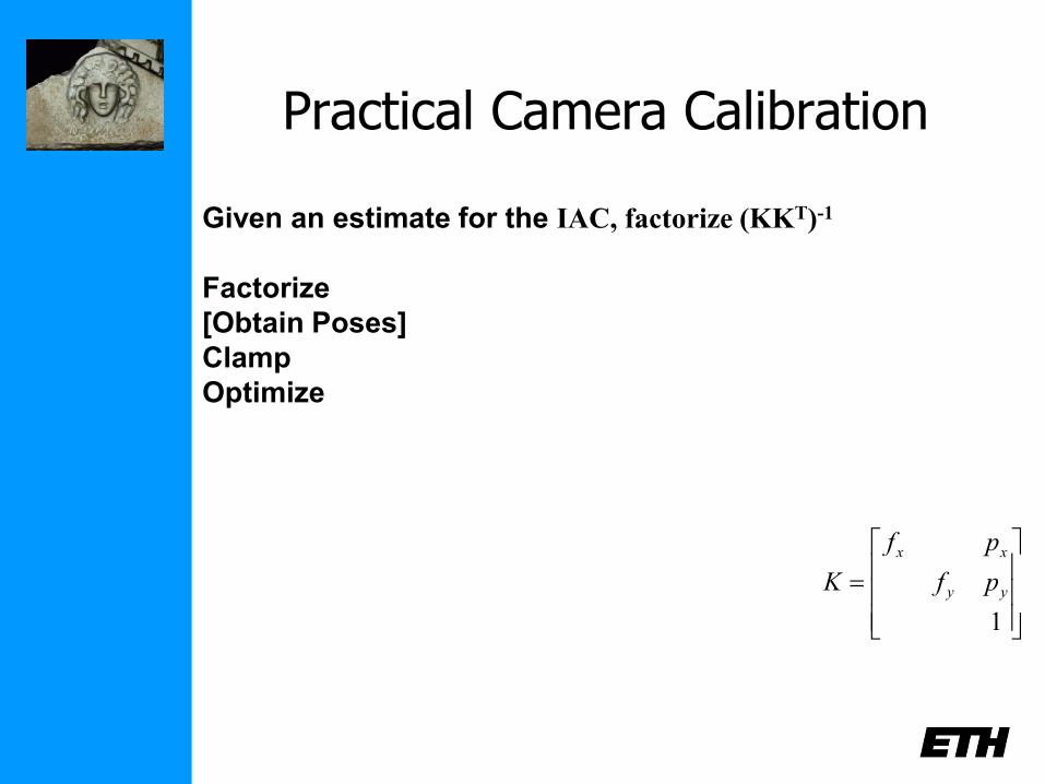
Given an estimate for the IAC, factorize (KKT)-1

Factorize

[Obtain Poses]

Clamp

Optimize

Reminder

• Project presentation in 2 weeks

• Find team mate / decide topic soon

• Limited number of kinects: first come, first served !