Embed Size (px)
DESCRIPTION
MyS Soldadura 1
Citation preview
SIMULATION
AND
MODELING Welding Esp.
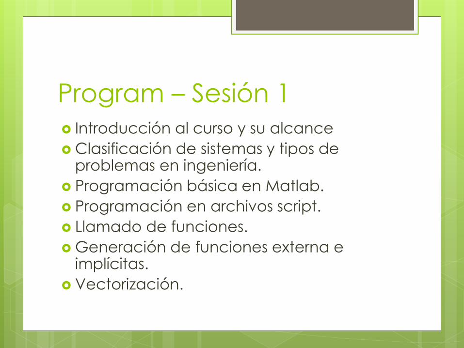
Program – Sesión 1
Introducción al curso y su alcance
Clasificación de sistemas y tipos de problemas en ingeniería.
Programación básica en Matlab.
Programación en archivos script.
Llamado de funciones.
Generación de funciones externa e implícitas.
Vectorización.
Bibliografía Klee, H. Simulation of Dynamic Systems With MATLAB
and Simulink. Ed CRC Press.
Ogata K. Dinámica de Sistemas. D. Prentice Hall.
Magrab E. An Engineer’s Guide to MATLAB.
Constantinides A. Numerical Methods for Chemical
Engineers with MATLAB Applications. Ed. Prentice
Hall.
Sesión 1: Introducción, alcance y
objetivos del curso.
El curso está encaminado a brindar herramientas
matemáticas y conceptuales para que el
estudiante pueda identificar las partes de un
sistema y empleando las leyes físicas y
constitutivas generar modelos matemáticos y
posteriormente numéricos de procesos afines a sus
áreas de estudio.
Por que el modelado y la
simulación.
Diferenciar:
Simular: EMULAR la realidad
Modelar: A partir de la observación del
fenómeno real y mediante algunas
suposiciones y SIMPLIFICACIONES se genera UN
MODELO que APROXIMADAMENTE representa
el problema real.
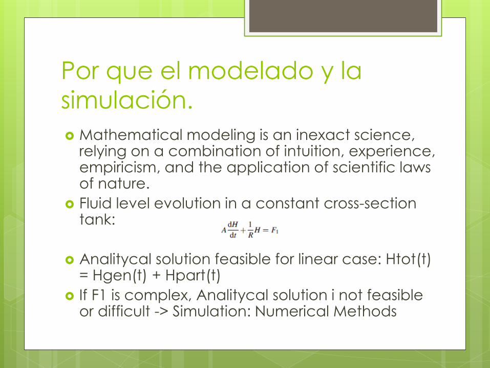
Por que el modelado y la
simulación.
Mathematical modeling is an inexact science, relying on a combination of intuition, experience, empiricism, and the application of scientific laws of nature.
Fluid level evolution in a constant cross-section tank:
Analitycal solution feasible for linear case: Htot(t) = Hgen(t) + Hpart(t)
If F1 is complex, Analitycal solution i not feasible or difficult -> Simulation: Numerical Methods

Un problema
“trivial”:
Determine los
esfuerzos
críticos en las
patas de la
sillas.

La solución analítica
puede ser un poco
“engorrosa”
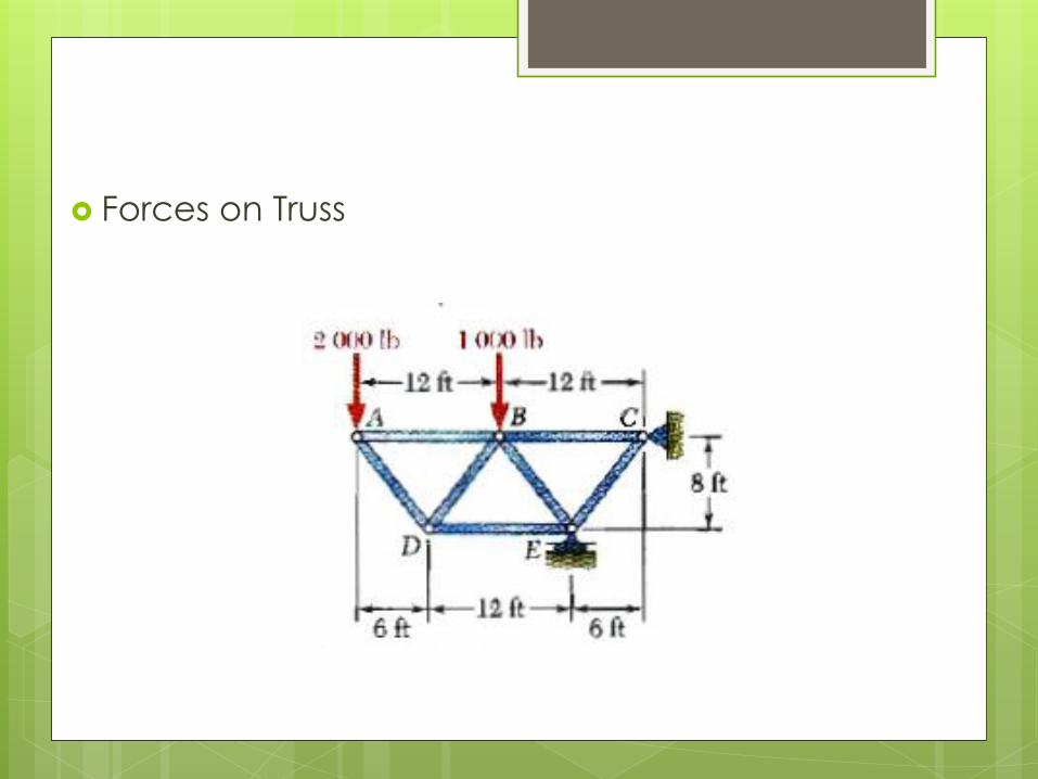
Forces on Truss
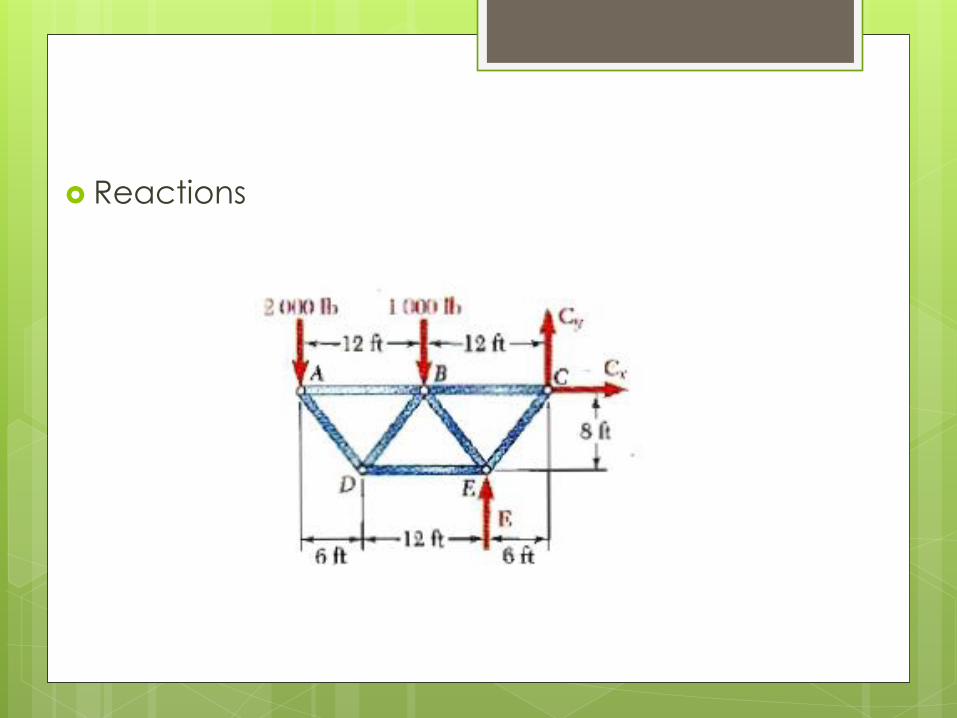
Reactions
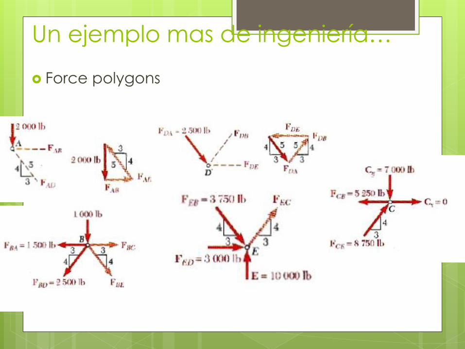
Un ejemplo mas de ingeniería…
Force polygons
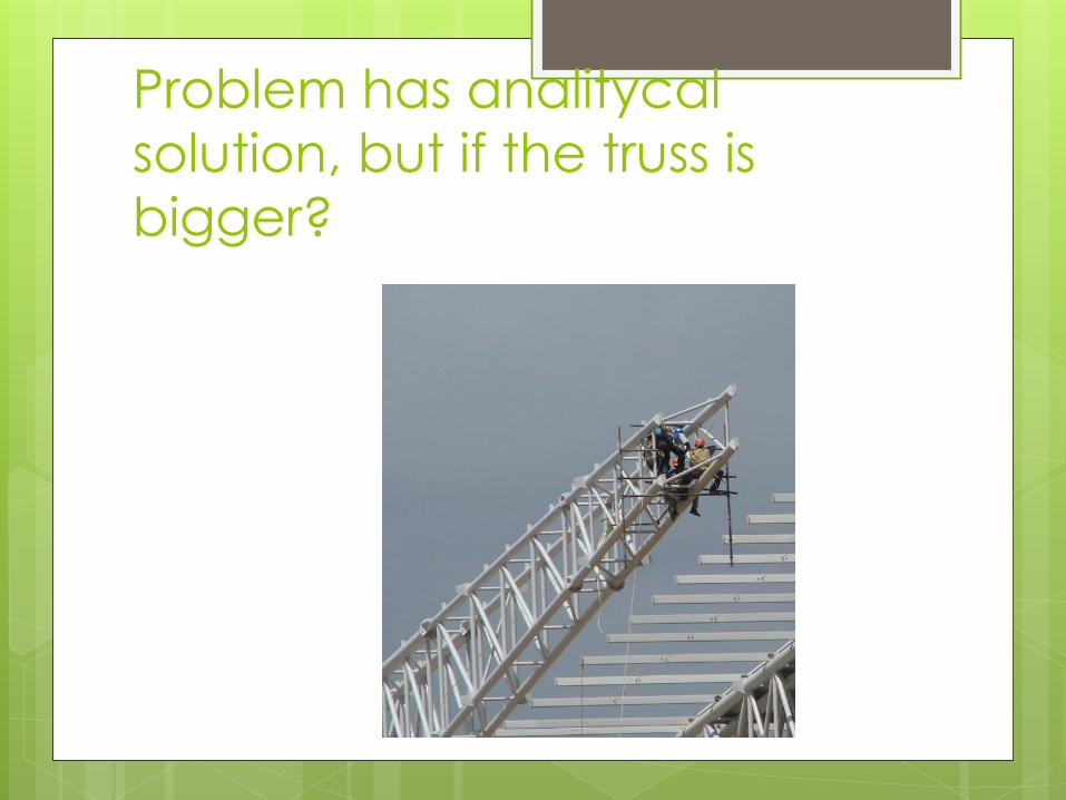
Problem has analitycal
solution, but if the truss is
bigger?
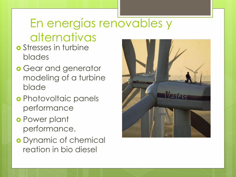
En energías renovables y
alternativas Stresses in turbine
blades
Gear and generator
modeling of a turbine
blade
Photovoltaic panels
performance
Power plant
performance.
Dynamic of chemical
reation in bio diesel
Conclusión. Algunas razones por las cuales el avance
tecnológico en prácticamente todas las áreas ha aumentado dramáticamente desde la aparición del computador son:
Aumento del poder de computo.
Aparición de nuevas teorías ý algoritmos para solución de problemas científicos y de ingeniería cada vez mas específicos y complejos.
Creación de códigos y software especializado.
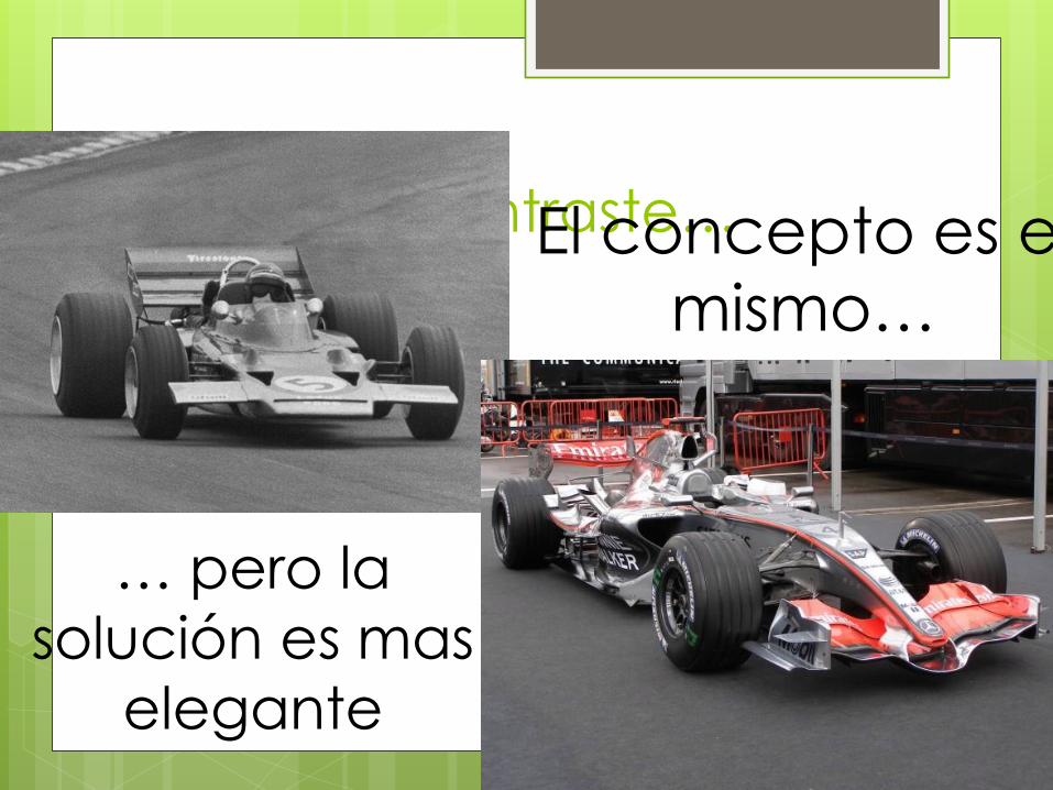
Un último contraste… El concepto es el
mismo…
… pero la
solución es mas
elegante
Clasificación de los tipos de
problemas y sistemas físicos Los sistemas (físicos, económicos, …) depende de:
El número de variables.
El comportamiento del sistema en el tiempo.
El grado de certidumbre de los parámetros y variables
del sistema.
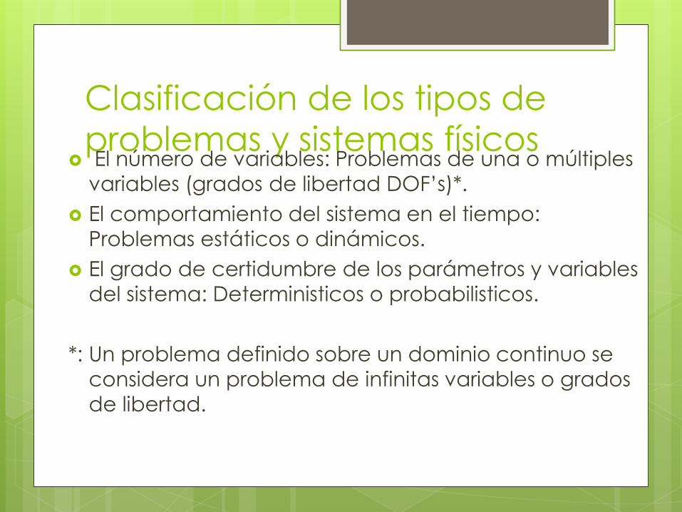
Clasificación de los tipos de
problemas y sistemas físicos El número de variables: Problemas de una o múltiples
variables (grados de libertad DOF’s)*.
El comportamiento del sistema en el tiempo:
Problemas estáticos o dinámicos.
El grado de certidumbre de los parámetros y variables
del sistema: Deterministicos o probabilisticos.
*: Un problema definido sobre un dominio continuo se
considera un problema de infinitas variables o grados
de libertad.
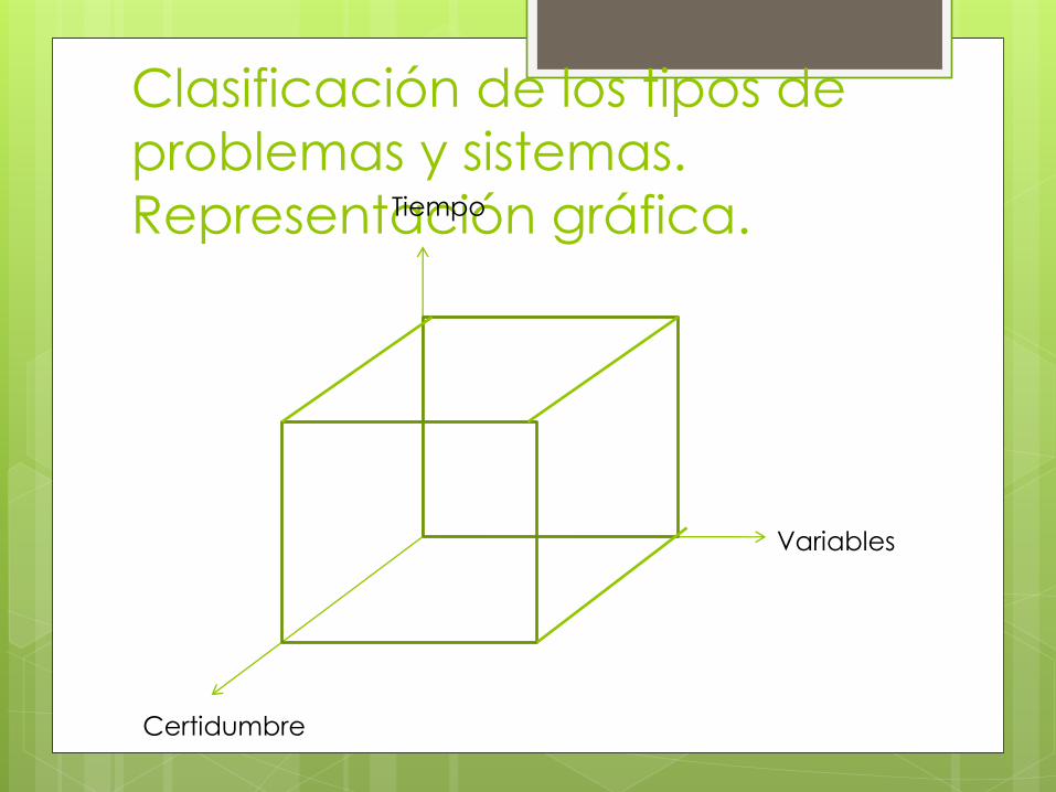
Clasificación de los tipos de
problemas y sistemas.
Representación gráfica.
Variables
Tiempo
Certidumbre
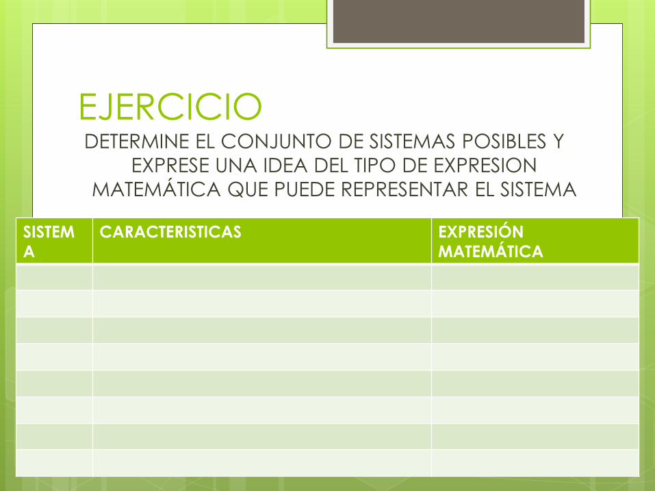
EJERCICIO DETERMINE EL CONJUNTO DE SISTEMAS POSIBLES Y
EXPRESE UNA IDEA DEL TIPO DE EXPRESION
MATEMÁTICA QUE PUEDE REPRESENTAR EL SISTEMA
SISTEM
A
CARACTERISTICAS EXPRESIÓN
MATEMÁTICA
Ejemplos de sistemas físicos
afines a la ingeniería.
Ejercicio en clase.
Enuncie problemas físicos y prácticos de ingeniería
que este en cada categoría.
Dar 3 ejemplos de problemas y sistemas para cada
categoría.
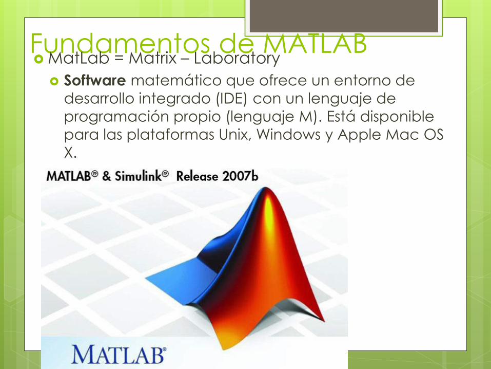
Fundamentos de MATLAB MatLab = Matrix – Laboratory
Software matemático que ofrece un entorno de
desarrollo integrado (IDE) con un lenguaje de
programación propio (lenguaje M). Está disponible
para las plataformas Unix, Windows y Apple Mac OS
X.
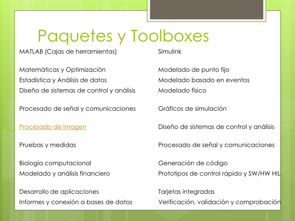
Paquetes y Toolboxes MATLAB (Cajas de herramientas) Simulink
Matemáticas y Optimización Modelado de punto fijo
Estadística y Análisis de datos Modelado basado en eventos
Diseño de sistemas de control y análisis Modelado físico
Procesado de señal y comunicaciones Gráficos de simulación
Procesado de imagen Diseño de sistemas de control y análisis
Pruebas y medidas Procesado de señal y comunicaciones
Biología computacional Generación de código
Modelado y análisis financiero Prototipos de control rápido y SW/HW HIL
Desarrollo de aplicaciones Tarjetas integradas
Informes y conexión a bases de datos Verificación, validación y comprobación
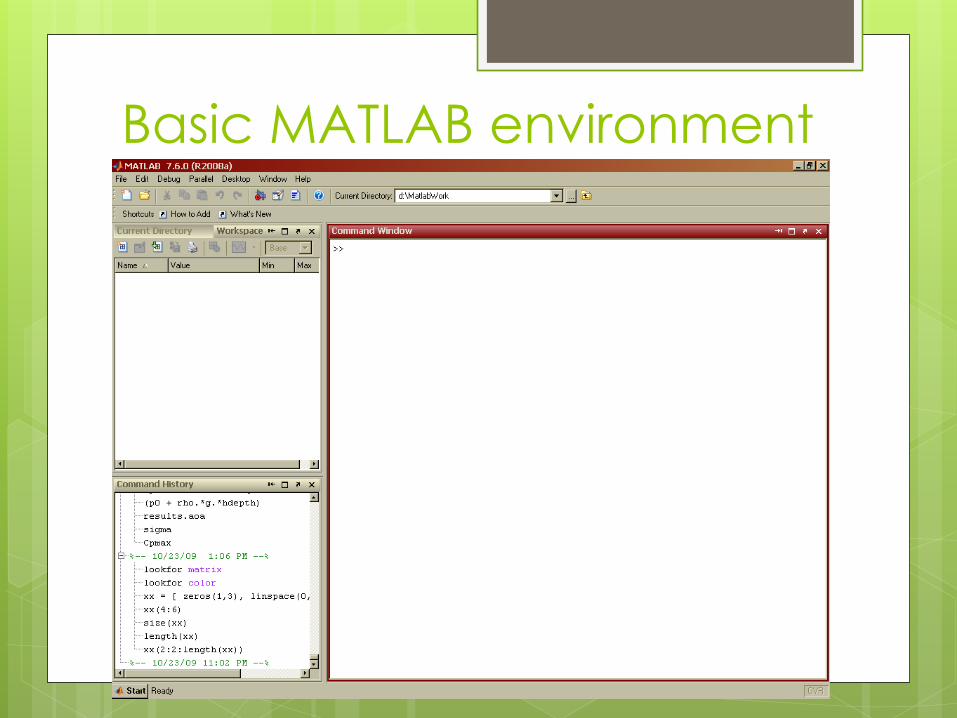
Basic MATLAB environment
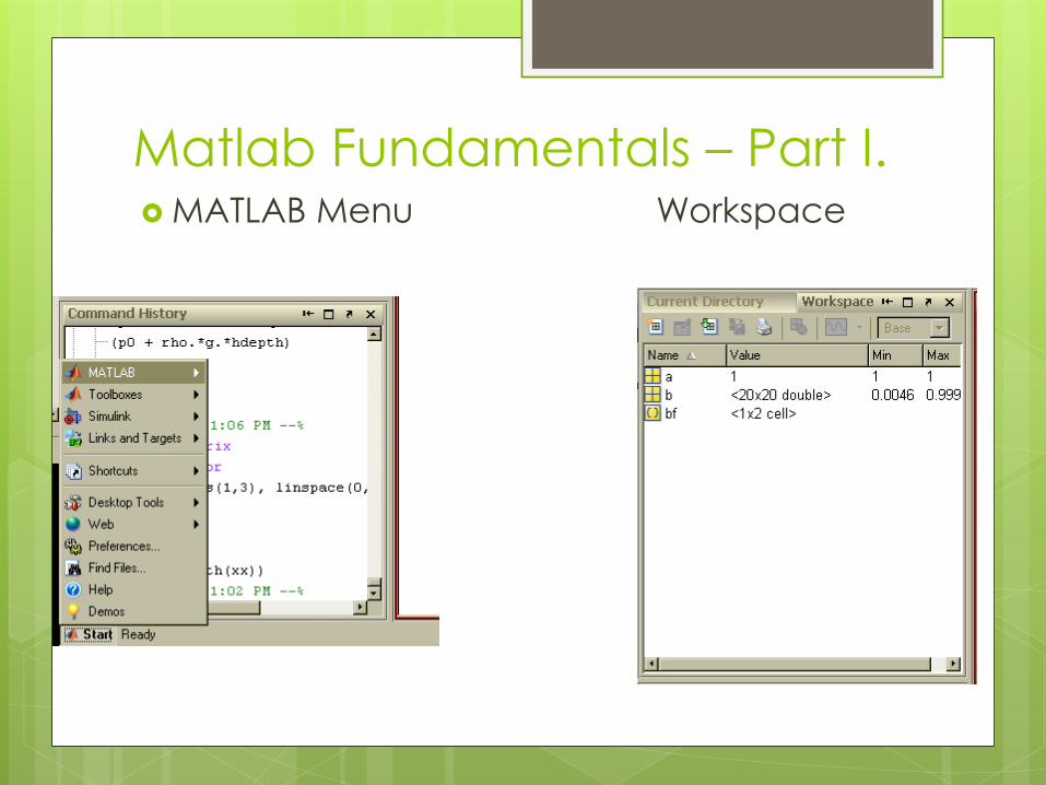
Matlab Fundamentals – Part I. MATLAB Menu Workspace
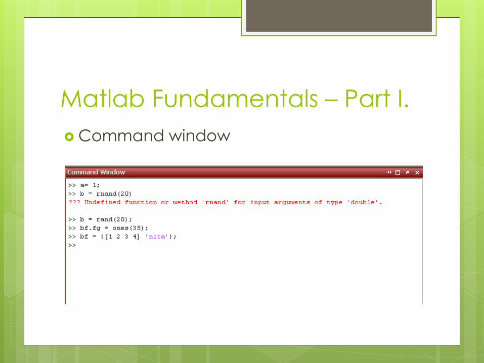
Matlab Fundamentals – Part I.
Command window
Matlab Fundamentals – Part I. The following exercises will begin your orientation in MATLAB. View the MATLAB introduction by typing intro at the MATLAB
prompt. This short introduction will demonstrate some of the basics of using MATLAB.
Explore the MATLAB help capability. Type each of the following lines to read about these commands: help
Help plot
Help colon
Help ops
Help zeros
Help ones
Lookfor filter kERWORD
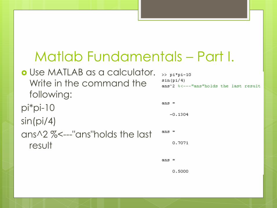
Matlab Fundamentals – Part I. Use MATLAB as a calculator.
Write in the command the
following:
pi*pi-10
sin(pi/4)
ans^2 %<---"ans"holds the last
result
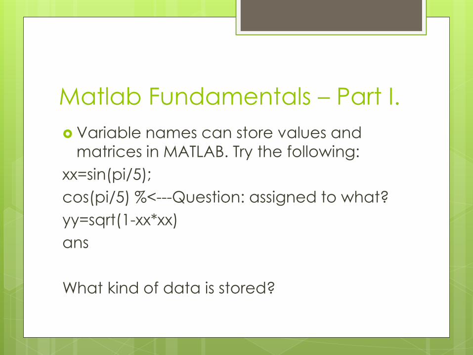
Matlab Fundamentals – Part I.
Variable names can store values and
matrices in MATLAB. Try the following:
xx=sin(pi/5);
cos(pi/5) %<---Question: assigned to what?
yy=sqrt(1-xx*xx)
ans
What kind of data is stored?

Matlab Fundamentals – Part I. The following exercises will begin your orientation in MATLAB. View the MATLAB introduction by typing intro at the MATLAB
prompt. This short introduction will demonstrate some of the basics of using MATLAB.
Explore the MATLAB help capability. Type each of the following lines to read about these commands: help
Help plot
Help colon
Help ops
Help zeros
Help ones
Lookfor filter kERWORD
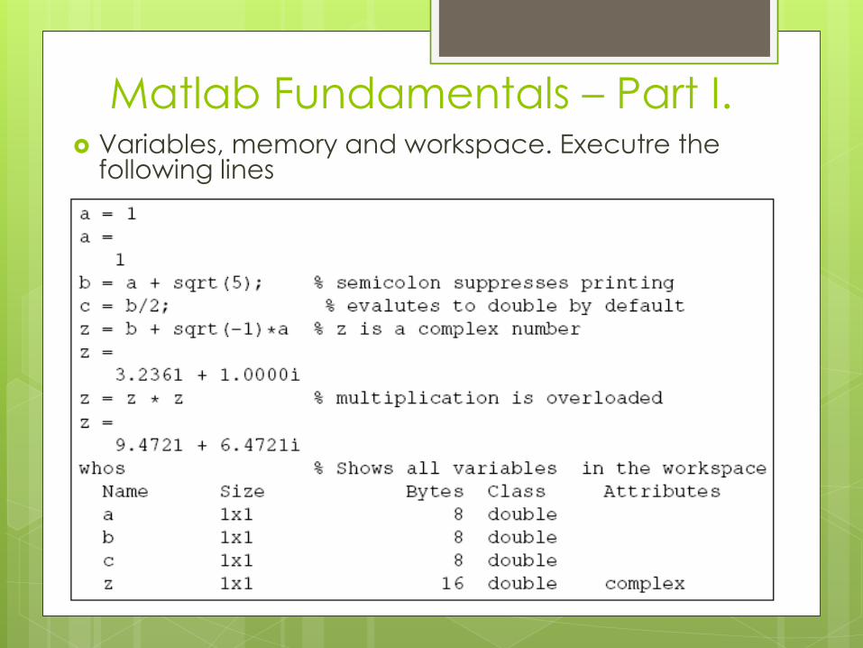
Matlab Fundamentals – Part I. Variables, memory and workspace. Executre the
following lines
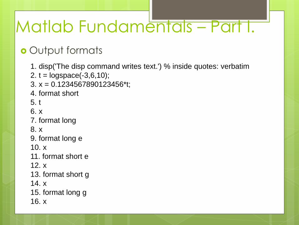
Matlab Fundamentals – Part I.
Output formats
1. disp('The disp command writes text.') % inside quotes: verbatim
2. t = logspace(-3,6,10);
3. x = 0.1234567890123456*t;
4. format short
5. t
6. x
7. format long
8. x
9. format long e
10. x
11. format short e
12. x
13. format short g
14. x
15. format long g
16. x
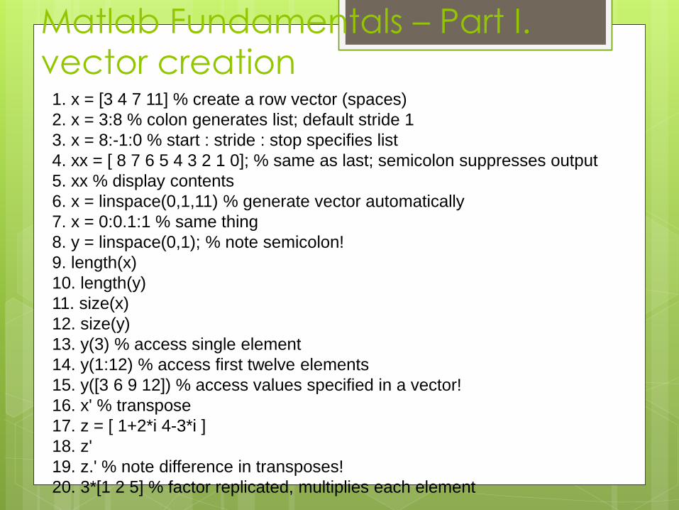
Matlab Fundamentals – Part I.
vector creation 1. x = [3 4 7 11] % create a row vector (spaces)
2. x = 3:8 % colon generates list; default stride 1
3. x = 8:-1:0 % start : stride : stop specifies list
4. xx = [ 8 7 6 5 4 3 2 1 0]; % same as last; semicolon suppresses output
5. xx % display contents
6. x = linspace(0,1,11) % generate vector automatically
7. x = 0:0.1:1 % same thing
8. y = linspace(0,1); % note semicolon!
9. length(x)
10. length(y)
11. size(x)
12. size(y)
13. y(3) % access single element
14. y(1:12) % access first twelve elements
15. y([3 6 9 12]) % access values specified in a vector!
16. x' % transpose
17. z = [ 1+2*i 4-3*i ]
18. z'
19. z.' % note difference in transposes!
20. 3*[1 2 5] % factor replicated, multiplies each element
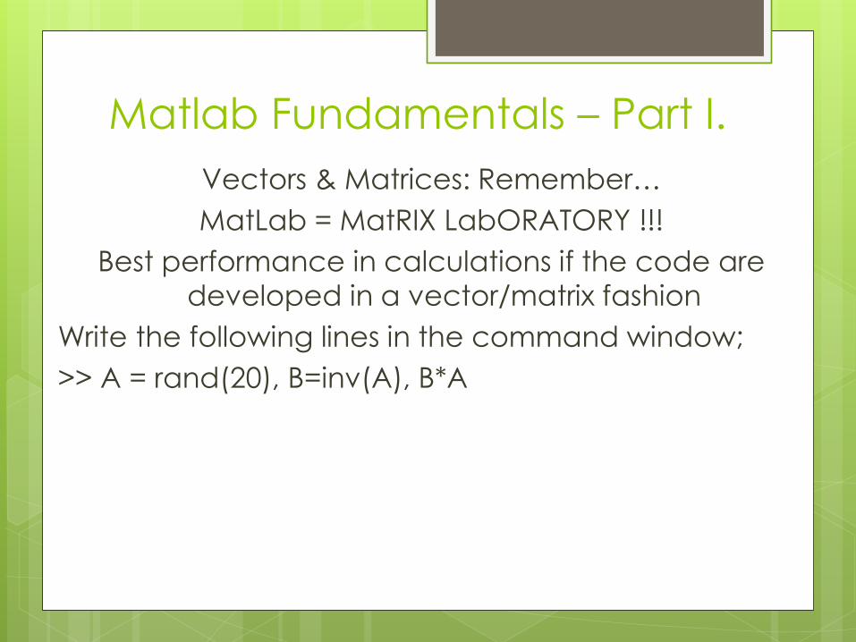
Matlab Fundamentals – Part I.
Vectors & Matrices: Remember…
MatLab = MatRIX LabORATORY !!!
Best performance in calculations if the code are
developed in a vector/matrix fashion
Write the following lines in the command window;
>> A = rand(20), B=inv(A), B*A
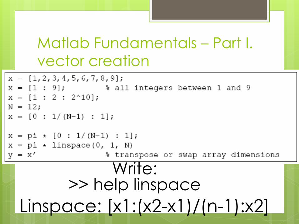
Matlab Fundamentals – Part I.
vector creation
Write: >> help linspace
Linspace: [x1:(x2-x1)/(n-1):x2]
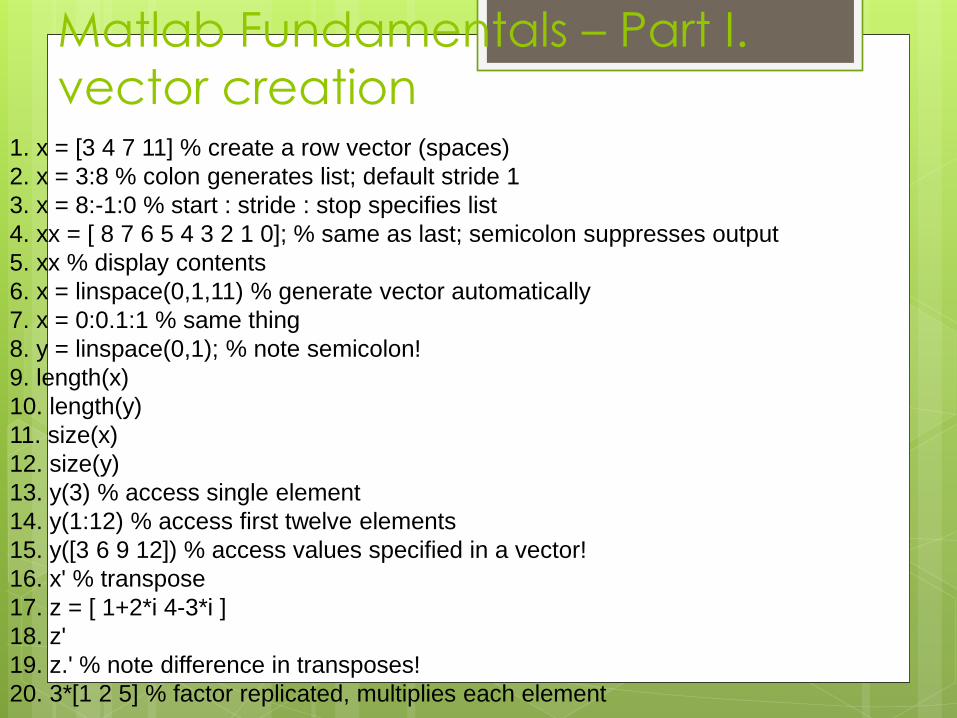
Matlab Fundamentals – Part I.
vector creation 1. x = [3 4 7 11] % create a row vector (spaces)
2. x = 3:8 % colon generates list; default stride 1
3. x = 8:-1:0 % start : stride : stop specifies list
4. xx = [ 8 7 6 5 4 3 2 1 0]; % same as last; semicolon suppresses output
5. xx % display contents
6. x = linspace(0,1,11) % generate vector automatically
7. x = 0:0.1:1 % same thing
8. y = linspace(0,1); % note semicolon!
9. length(x)
10. length(y)
11. size(x)
12. size(y)
13. y(3) % access single element
14. y(1:12) % access first twelve elements
15. y([3 6 9 12]) % access values specified in a vector!
16. x' % transpose
17. z = [ 1+2*i 4-3*i ]
18. z'
19. z.' % note difference in transposes!
20. 3*[1 2 5] % factor replicated, multiplies each element
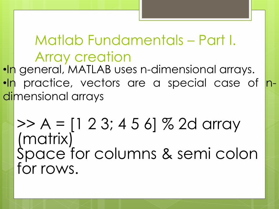
Matlab Fundamentals – Part I.
Array creation •In general, MATLAB uses n-dimensional arrays.
•In practice, vectors are a special case of n-
dimensional arrays
>> A = [1 2 3; 4 5 6] % 2d array (matrix) Space for columns & semi colon for rows.
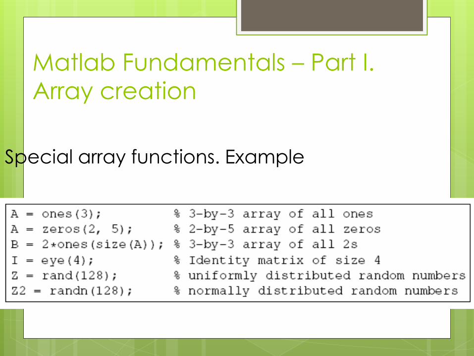
Matlab Fundamentals – Part I.
Array creation
Special array functions. Example
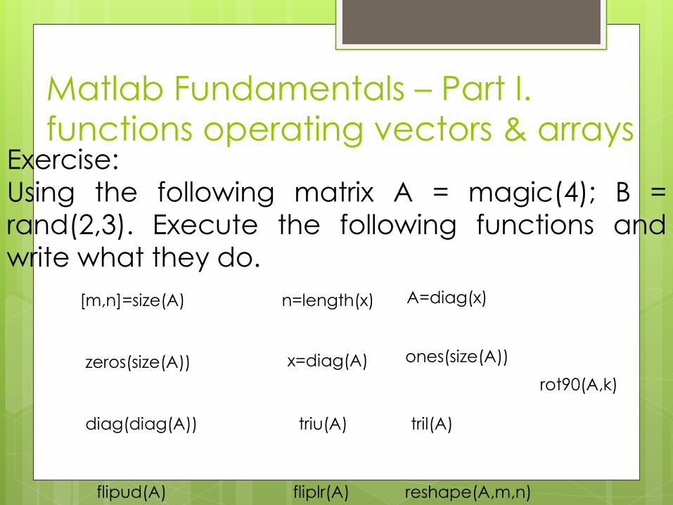
Matlab Fundamentals – Part I.
functions operating vectors & arrays Exercise:
Using the following matrix A = magic(4); B =
rand(2,3). Execute the following functions and write what they do.
[m,n]=size(A) n=length(x)
zeros(size(A)) ones(size(A))
A=diag(x)
x=diag(A)
diag(diag(A)) triu(A) tril(A)
rot90(A,k)
flipud(A) fliplr(A) reshape(A,m,n)
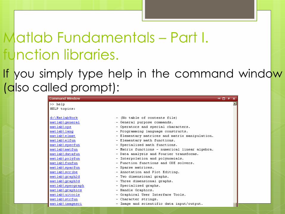
Matlab Fundamentals – Part I.
function libraries.
If you simply type help in the command window
(also called prompt):
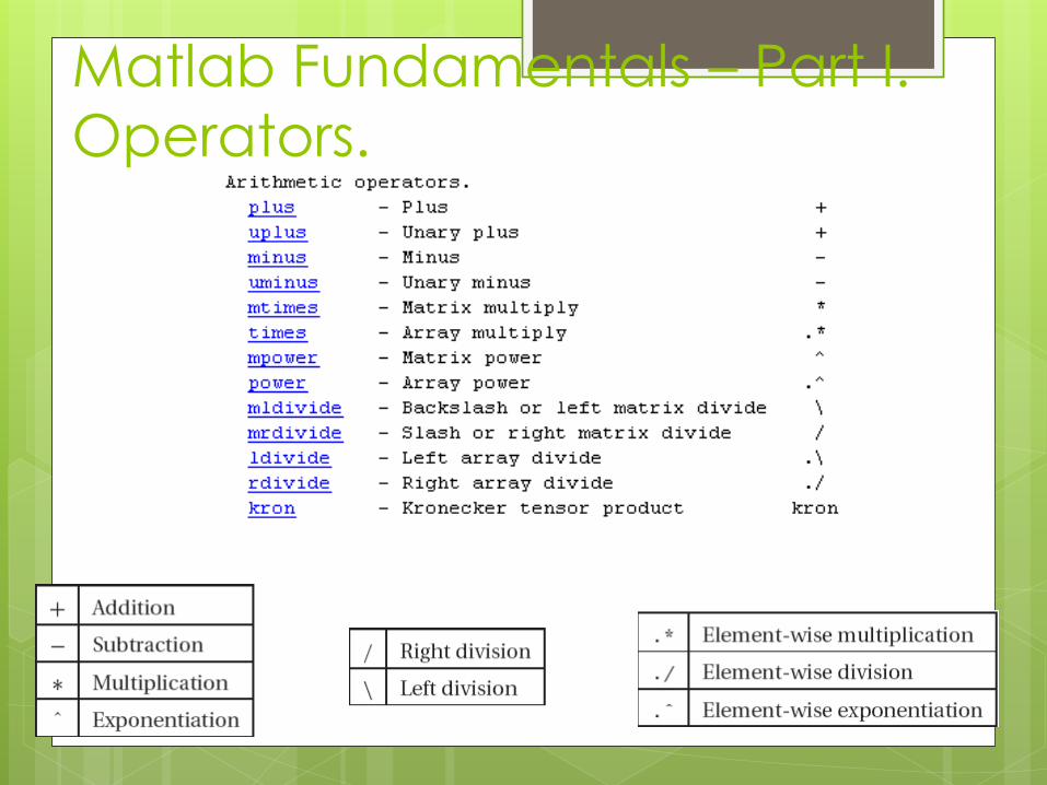
Matlab Fundamentals – Part I.
Operators.
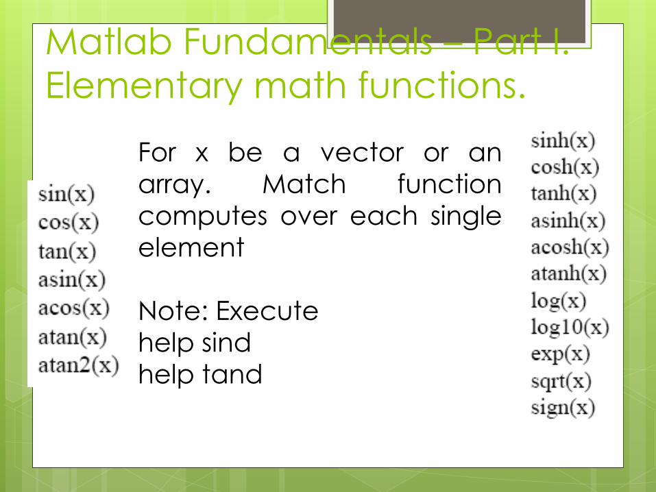
Matlab Fundamentals – Part I.
Elementary math functions.
For x be a vector or an
array. Match function
computes over each single element
Note: Execute help sind
help tand
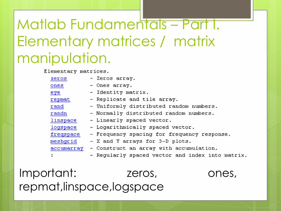
Matlab Fundamentals – Part I.
Elementary matrices / matrix
manipulation.
Important: zeros, ones, eye, repmat,linspace,logspace
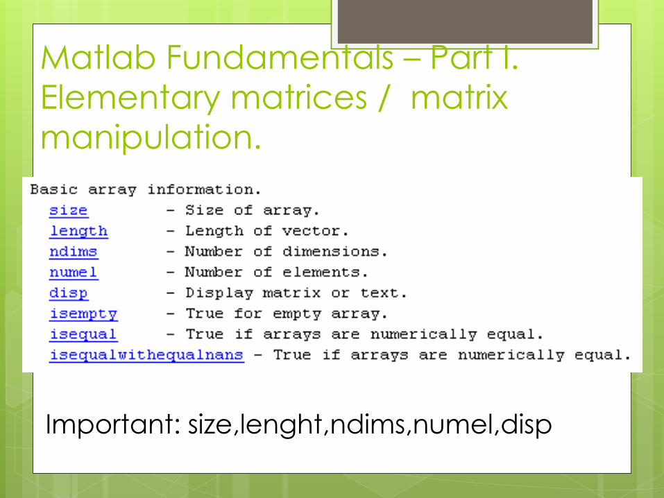
Matlab Fundamentals – Part I.
Elementary matrices / matrix
manipulation.
Important: size,lenght,ndims,numel,disp
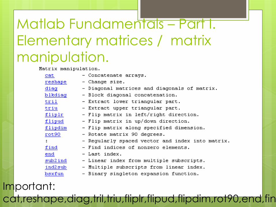
Matlab Fundamentals – Part I.
Elementary matrices / matrix
manipulation.
Important:
cat,reshape,diag,tril,triu,fliplr,flipud,flipdim,rot90,end,find
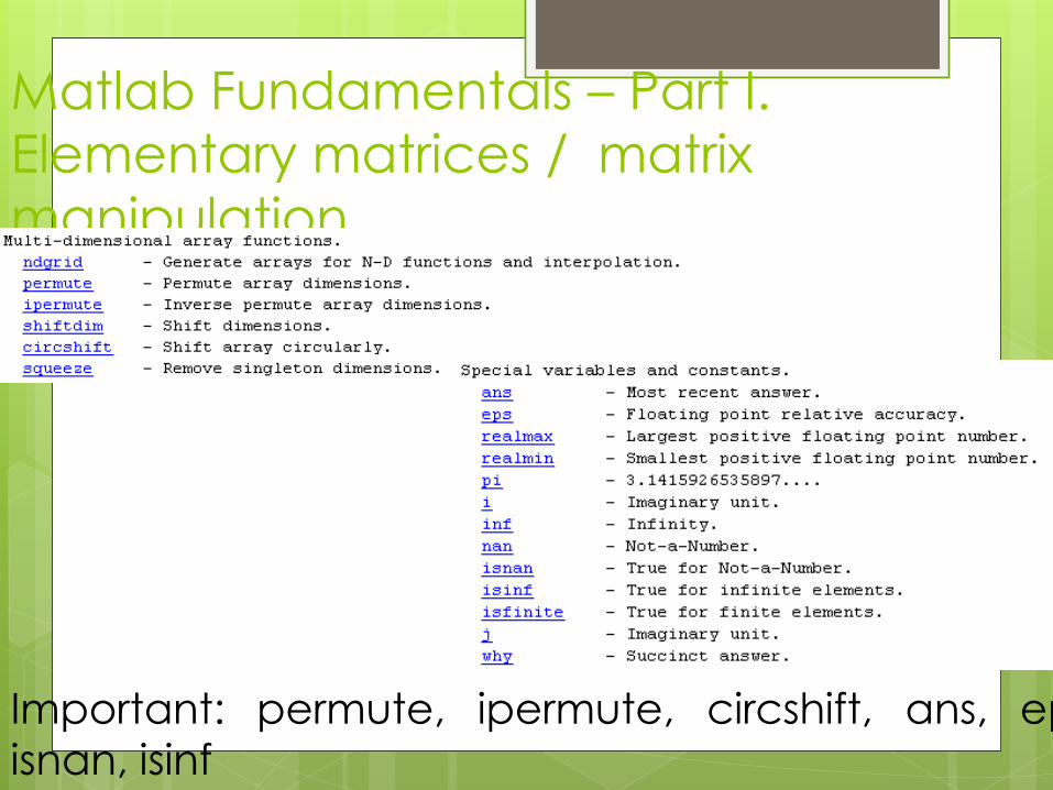
Matlab Fundamentals – Part I.
Elementary matrices / matrix
manipulation.
Important: permute, ipermute, circshift, ans, eps,
isnan, isinf
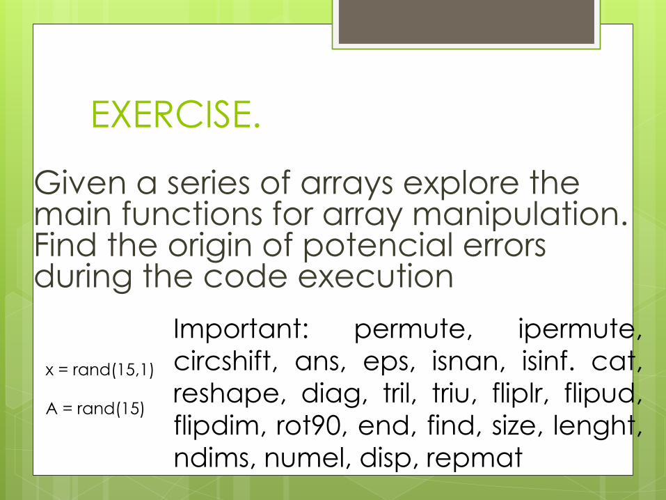
EXERCISE.
Given a series of arrays explore the main functions for array manipulation. Find the origin of potencial errors during the code execution
x = rand(15,1)
A = rand(15)
Important: permute, ipermute, circshift, ans, eps, isnan, isinf. cat,
reshape, diag, tril, triu, fliplr, flipud,
flipdim, rot90, end, find, size, lenght,
ndims, numel, disp, repmat
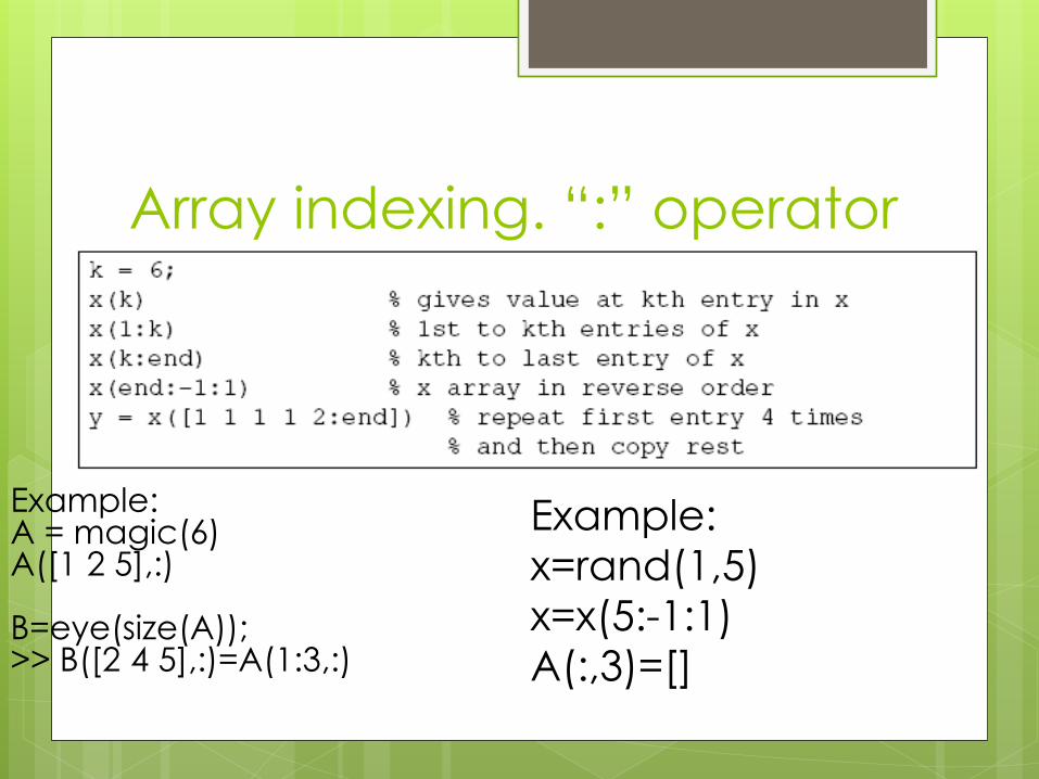
Array indexing. “:” operator
Example: A = magic(6) A([1 2 5],:)
B=eye(size(A)); >> B([2 4 5],:)=A(1:3,:)
Example: x=rand(1,5)
x=x(5:-1:1)
A(:,3)=[]
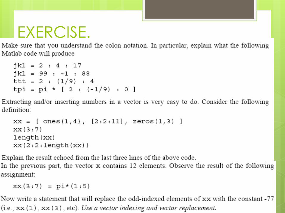
EXERCISE.
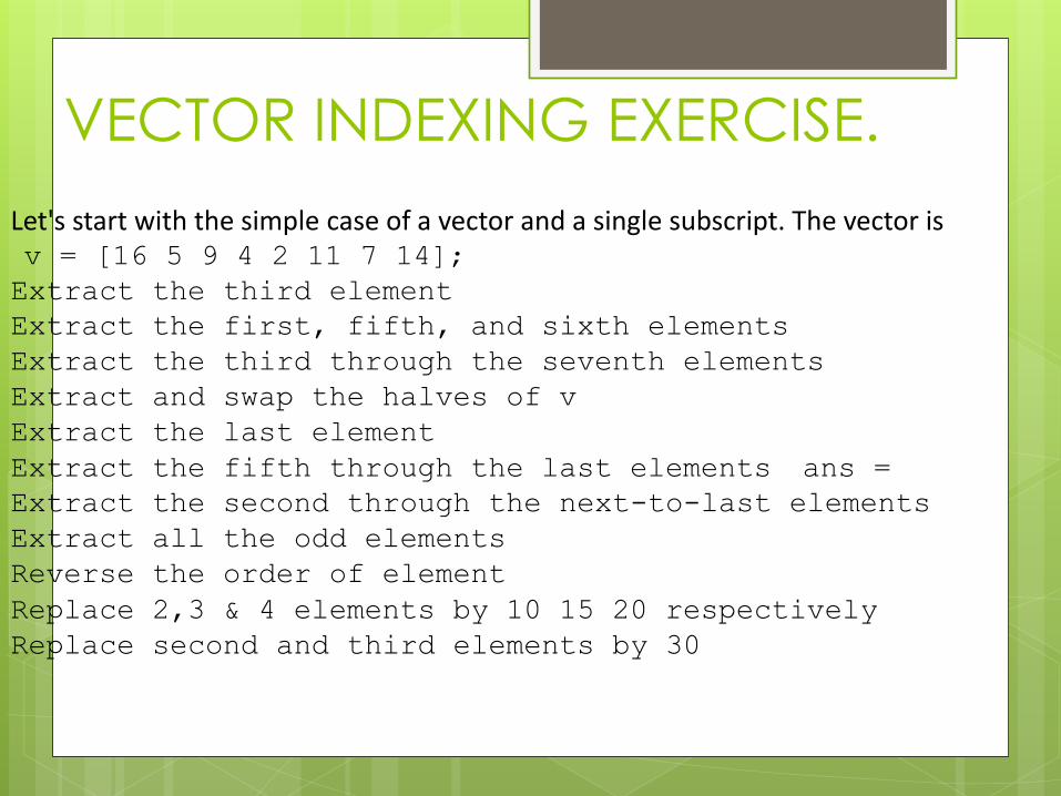
VECTOR INDEXING EXERCISE.
Let's start with the simple case of a vector and a single subscript. The vector is v = [16 5 9 4 2 11 7 14]; Extract the third element Extract the first, fifth, and sixth elements
Extract the third through the seventh elements
Extract and swap the halves of v
Extract the last element
Extract the fifth through the last elements ans = Extract the second through the next-to-last elements
Extract all the odd elements
Reverse the order of element
Replace 2,3 & 4 elements by 10 15 20 respectively
Replace second and third elements by 30
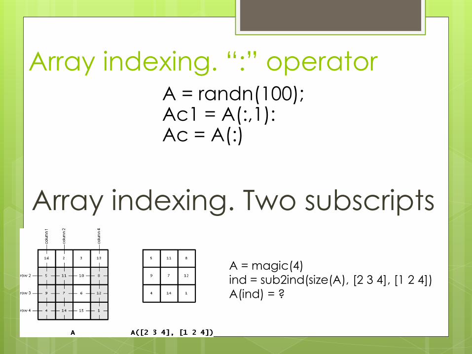
Array indexing. “:” operator A = randn(100); Ac1 = A(:,1): Ac = A(:) Array indexing. Two subscripts
A = magic(4)
ind = sub2ind(size(A), [2 3 4], [1 2 4])
A(ind) = ?
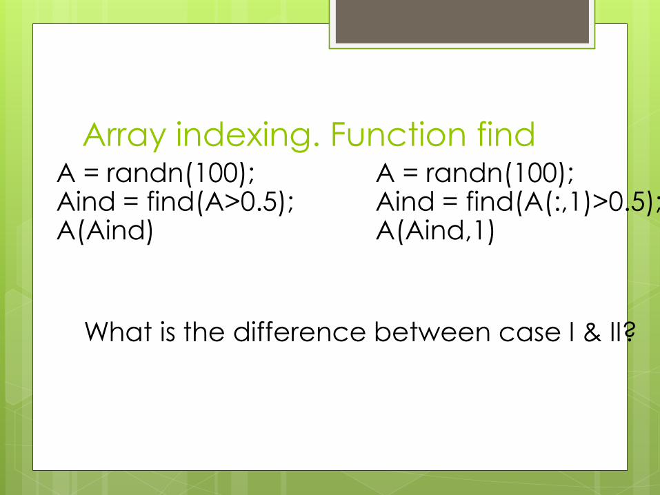
Array indexing. Function find A = randn(100); Aind = find(A>0.5); A(Aind)
A = randn(100); Aind = find(A(:,1)>0.5); A(Aind,1)
What is the difference between case I & II?
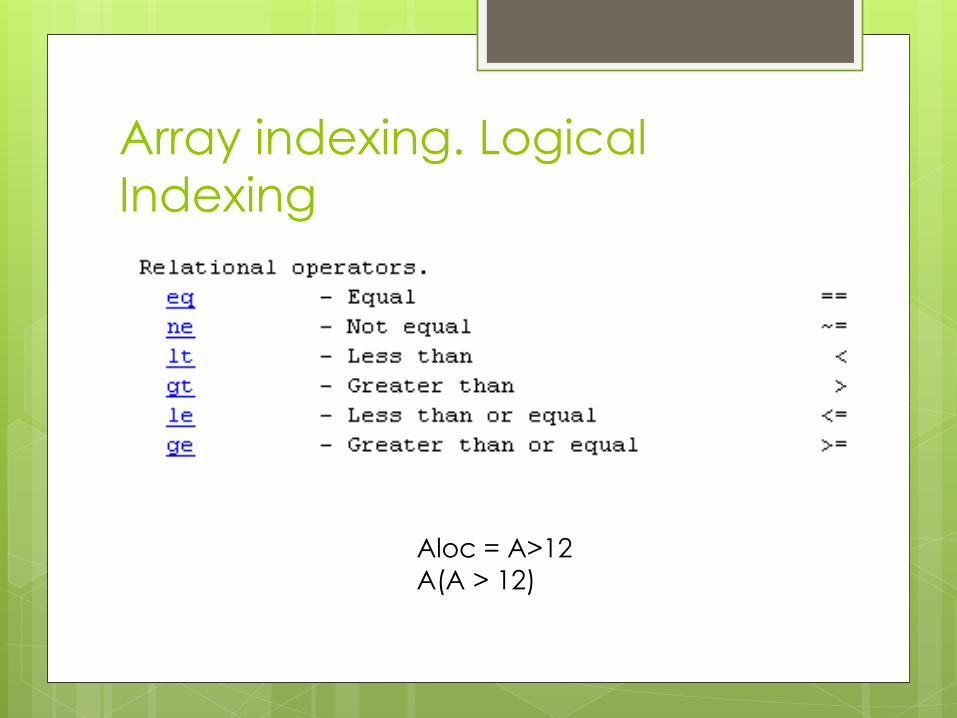
Array indexing. Logical
Indexing
Aloc = A>12
A(A > 12)
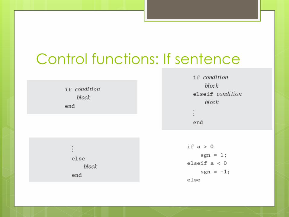
Control functions: If sentence
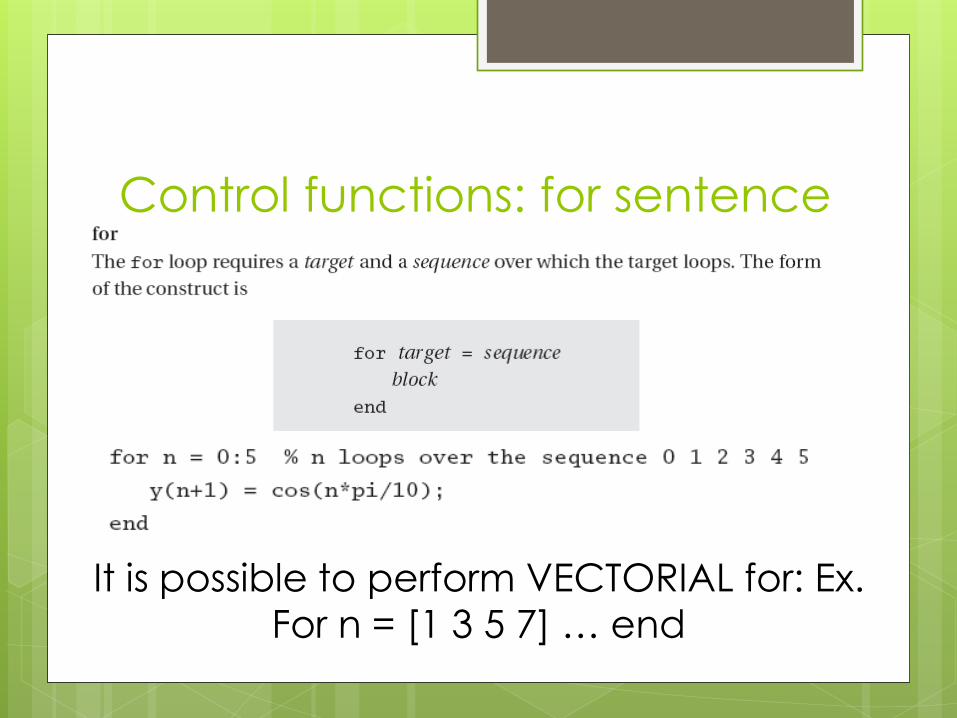
Control functions: for sentence
It is possible to perform VECTORIAL for: Ex. For n = [1 3 5 7] … end
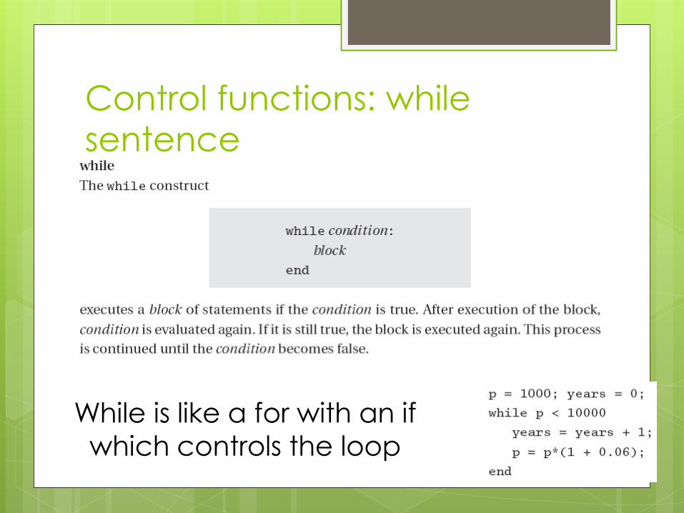
Control functions: while
sentence
While is like a for with an if which controls the loop
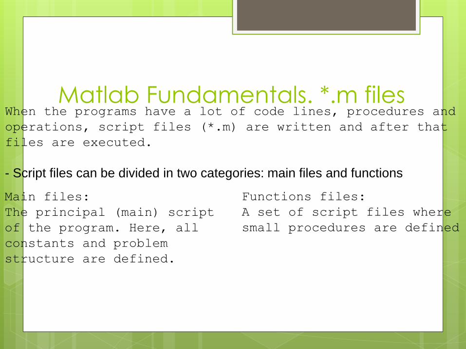
Matlab Fundamentals. *.m files When the programs have a lot of code lines, procedures and
operations, script files (*.m) are written and after that
files are executed.
- Script files can be divided in two categories: main files and functions
Main files:
The principal (main) script
of the program. Here, all
constants and problem
structure are defined.
Functions files:
A set of script files where
small procedures are defined
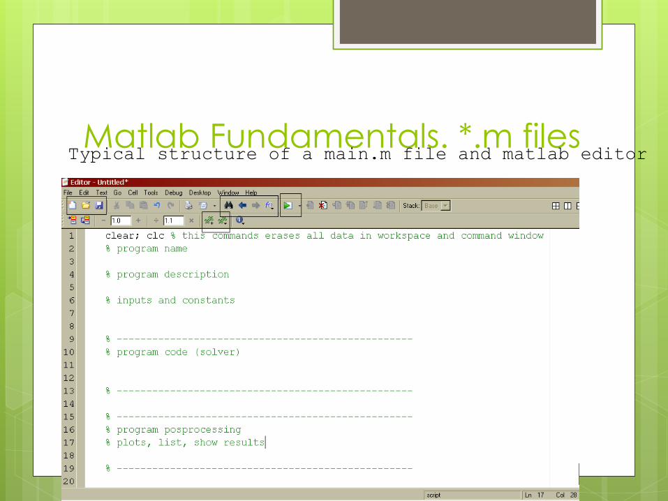
Matlab Fundamentals. *.m files Typical structure of a main.m file and matlab editor
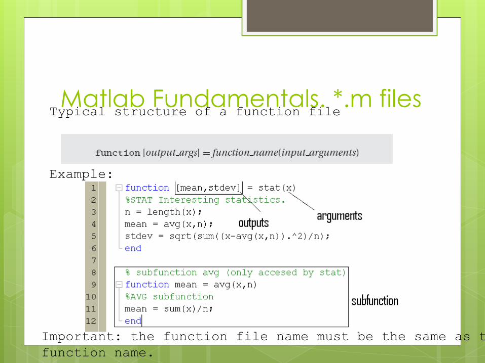
Matlab Fundamentals. *.m files Typical structure of a function file
Example:
Important: the function file name must be the same as the
function name.
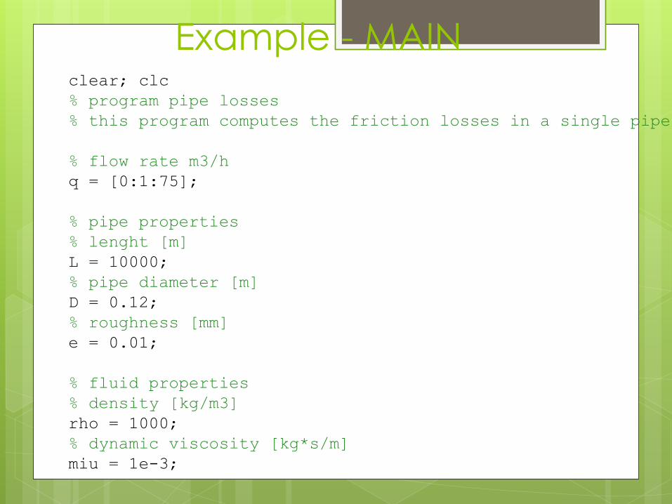
Example - MAIN clear; clc
% program pipe losses
% this program computes the friction losses in a single pipe
% flow rate m3/h
q = [0:1:75];
% pipe properties
% lenght [m]
L = 10000;
% pipe diameter [m]
D = 0.12;
% roughness [mm]
e = 0.01;
% fluid properties
% density [kg/m3]
rho = 1000;
% dynamic viscosity [kg*s/m]
miu = 1e-3;
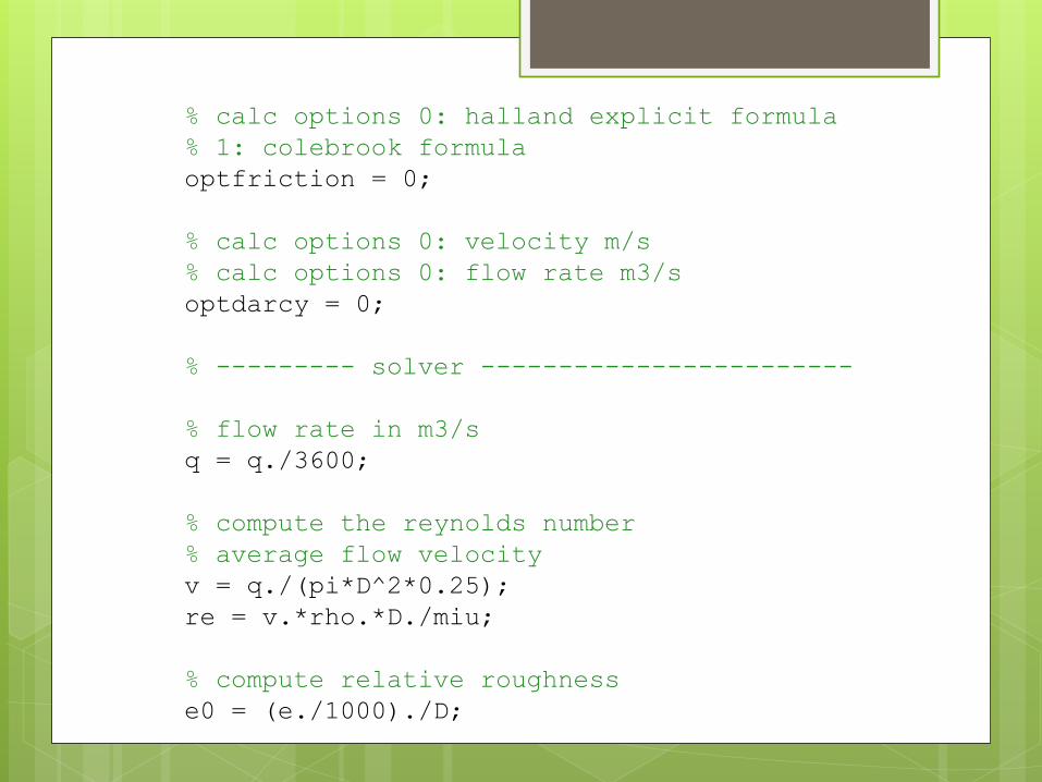
% calc options 0: halland explicit formula
% 1: colebrook formula
optfriction = 0;
% calc options 0: velocity m/s
% calc options 0: flow rate m3/s
optdarcy = 0;
% --------- solver ------------------------
% flow rate in m3/s
q = q./3600;
% compute the reynolds number
% average flow velocity
v = q./(pi*D^2*0.25);
re = v.*rho.*D./miu;
% compute relative roughness
e0 = (e./1000)./D;
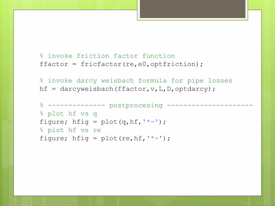
% invoke friction factor function
ffactor = fricfactor(re,e0,optfriction);
% invoke darcy weisbach formula for pipe losses
hf = darcyweisbach(ffactor,v,L,D,optdarcy);
% -------------- postprocesing ---------------------
% plot hf vs q
figure; hfig = plot(q,hf,'*-');
% plot hf vs re
figure; hfig = plot(re,hf,'*-');
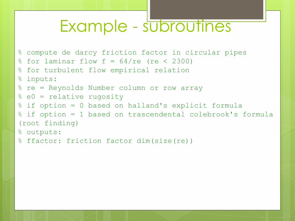
Example - subroutines
% compute de darcy friction factor in circular pipes
% for laminar flow f = 64/re (re < 2300)
% for turbulent flow empirical relation
% inputs:
% re = Reynolds Number column or row array
% e0 = relative rugosity
% if option = 0 based on halland's explicit formula
% if option = 1 based on trascendental colebrook's formula
(root finding)
% outputs:
% ffactor: friction factor dim(size(re))
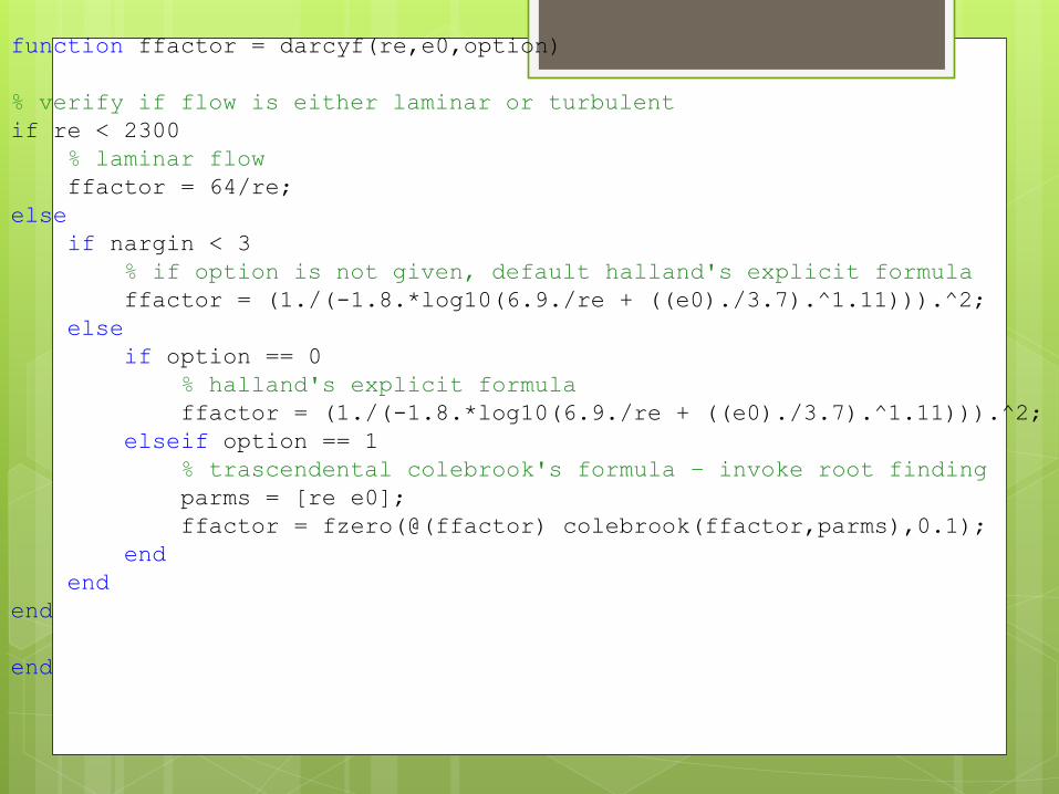
function ffactor = darcyf(re,e0,option)
% verify if flow is either laminar or turbulent
if re < 2300
% laminar flow
ffactor = 64/re;
else
if nargin < 3
% if option is not given, default halland's explicit formula
ffactor = (1./(-1.8.*log10(6.9./re + ((e0)./3.7).^1.11))).^2;
else
if option == 0
% halland's explicit formula
ffactor = (1./(-1.8.*log10(6.9./re + ((e0)./3.7).^1.11))).^2;
elseif option == 1
% trascendental colebrook's formula – invoke root finding
parms = [re e0];
ffactor = fzero(@(ffactor) colebrook(ffactor,parms),0.1);
end
end
end
end
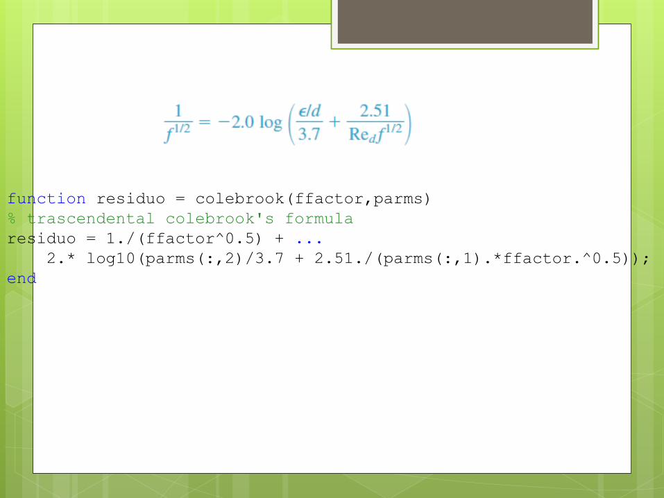
function residuo = colebrook(ffactor,parms)
% trascendental colebrook's formula
residuo = 1./(ffactor^0.5) + ...
2.* log10(parms(:,2)/3.7 + 2.51./(parms(:,1).*ffactor.^0.5));
end