TitleNew Directions in Exact Renormalization Group :Lifshitz-Type Theory, Gradient Flow Equation andIts Supersymmetric Extension

Author(s) 菊地, 健吾

Citation

Issue Date

Text Version ETD

URL https://doi.org/10.18910/50466

DOI 10.18910/50466

rights

New Directions in Exact Renormalization

Group: Lifshitz-Type Theory, Gradient Flow

Equation and Its Supersymmetric Extension

Kengo Kikuchi

Department of Physics, Graduate School of Science,

Osaka University, Toyonaka, 560-0043, Japan

A Dissertation for the degree of Doctor of Philosophy

May 9, 2014

Abstract

The purpose of this thesis is to present our study on the new direc-tions in the exact renormalization group (ERG) through the Lifshitz-type theory, the gradient flow equation and its supersymmetric ex-tension. There are two topics in this thesis. The first topic is thestudy on the restoration of the Lorentz symmetry for a Lifshitz-typescalar theory in the infrared region using non-perturbative methods.We apply the Wegner-Houghton equation, which is one of the exactrenormalization group equations, to the Lifshitz-type theory. Analyz-ing the equation for a z = 2, d = 3 + 1 Lifshitz-type scalar model,we find that symmetry violating terms vanish in the infrared region.This shows that the Lifshitz-type scalar model dynamically restoresthe Lorentz symmetry at low energy. Our result provides a definitionof ultraviolet complete renormalizable scalar field theories. These the-ories can have nontrivial interaction terms of φn(n = 4, 6, 8, 10) evenwhen the Lorentz symmetry is restored at low energy. The secondtopic is the gradient flow equation and its supersymmetric extension.We explain the expectation value in terms of a gauge field, which isdefined by a certain type of diffusion equation called a gradient flowequation, is finite without additional renormalization as a review. Andwe extend the equation to super Yang-Mills theory. We propose a gra-dient flow based on superfield formalism. As a result, we constructa supersymmetric extension of the gradient flow equation, which in-cludes only finite terms in the Wess-Zumino gauge. Our result alsoprovide the gradient flow equation of the matter field very naturally.Our studies could be an important step towards the ERG which keepsthe symmetry explicitly.

2

Contents

1 Introduction 6

I Restoration of Lorentz Symmetry for Lifshitz-TypeScalar Theory 11

2 Lifshitz-Type Theory 11

3 Extended Wegner-Houghton Equation for Lifshitz-Type The-

ory 12

4 Models and Analysis 13

4.1 z = 2, d = 3 + 1 Lifshitz-Type Scalar Model . . . . . . . . . . 13

4.2 Transformation of Variables . . . . . . . . . . . . . . . . . . . 17

5 Numerical Analysis 20

6 Short Summary 24

II Gradient Flow Equation and Its SupersymmetricExtension 26

7 Review of Gradient Flow Equation of Yang-Mills Theory 26

7.1 Definition of Gradient Flow Equation . . . . . . . . . . . . . . 27

7.2 Luscher-Weisz Theorem . . . . . . . . . . . . . . . . . . . . . 27

7.3 Energy Density . . . . . . . . . . . . . . . . . . . . . . . . . . 29

7.4 Applications of Gradient Flow Equation . . . . . . . . . . . . 30

7.4.1 Chiral Condensate . . . . . . . . . . . . . . . . . . . . 30

7.4.2 Small Flow Time Expansion . . . . . . . . . . . . . . . 31

7.4.3 Step Scaling and Improved Action . . . . . . . . . . . . 32

8 Supersymmetric Gradient Flow Equation 33

8.1 Our Proposal for Supersymmetric Gradient Flow Equation . . 34

3

9 Pure Abelian Supersymmetric Theory 35

9.1 Derivation of Gradient Flow Equation of Pure Abelian Super-

symmetric Theory . . . . . . . . . . . . . . . . . . . . . . . . 36

9.2 Gradient Flow Equation of Pure Yang-Mills Theory for Each

Component of Vector Multiplet . . . . . . . . . . . . . . . . . 37

9.3 Flow Time Dependence of Super Gauge Transformation . . . . 38

10 Super Yang-Mills Theory 39

10.1 Derivation of Gradient Flow Equation for Super Yang-Mills

Theory . . . . . . . . . . . . . . . . . . . . . . . . . . . . . . . 39

10.2 Gradient Flow Equation in Super Yang-Mills Theory under

Wess-Zumino Gauge . . . . . . . . . . . . . . . . . . . . . . . 40

10.2.1 Determination of Gauge Covariant Term . . . . . . . . 40

10.2.2 Determination of α0 Term . . . . . . . . . . . . . . . . 42

10.3 Gradient Flow Equation of Super Yang-Mills Theory for Each

Component of Vector Multiplet . . . . . . . . . . . . . . . . . 43

11 Short Summary 45

12 Summary and Disucussion 47

A Notation in Part. I 50

B Derivation of Wegner-Houghton Equation 50

C Notation in Part. II 53

D Solution of Gradient Flow Equation 54

E Short Summary of Supersymmetry 56

E.1 Definition . . . . . . . . . . . . . . . . . . . . . . . . . . . . . 56

E.2 Wess-Zumino Gauge . . . . . . . . . . . . . . . . . . . . . . . 56

F Derivation of Gauge Covariant Term 57

G Expansion of Equation (10.8) with Component Fields 59

G.1 Coordinate Transformation . . . . . . . . . . . . . . . . . . . . 59

4

G.2 Useful Formulae . . . . . . . . . . . . . . . . . . . . . . . . . . 60

5

1 Introduction

The goal of the elementary particle physics is to explain macroscopic phe-

nomena from the fundamental microscopic theory. We know that gauge

theories can describe phenomena which involve strong and electroweak in-

teractions. As is well known, however, the theory encounters ultraviolet

divergences. It is not so easy to avoid the divergences. For example, the

higher-dimensional gauge theory which is typified by physics beyond the

standard model is also perturbatively unrenormalizable. In 1940’s the the-

ory of perturbative renormalization, originally invented as a prescription to

avoid the divergence, contributed to quantum electrodynamics (QED) which

has lead to enormous success to date. However the perturbation theory is

not enough to understand physics. The non-perturbative approach is also

needed to explain strong coupling theories such as quantum chromodynam-

ics (QCD).

We are especially interested in the exact renormalization group (ERG),

which is one of the methods to analyze the physical system non-perturbatively.

In 1970’s, Wilson and Kogut gave a physical meaning to the renormalization

method, and constructed the framework of the ERG [1]. The philosophy

of the ERG is encoded in the formulation itself. We integrate out the high

frequency mode of the action and define the resulting action for the low fre-

quency mode as the Wilson effective action. The ERG equation gives the

change of the Wilson effective action as one changes the cut-off scale. The

ERG is not just a tool, but a powerful physical approach. One can even say

that knowing the renormalization group (RG) flow in the whole theory space

is equal to understanding the entire property of the physical system.

There are several different formulations for the ERG which exploit dif-

ferent cut-off functions or calculational methods, e.g. the Wegner-Houghton

equation, the Polchinski equation and the Wetterich equation. However be-

cause of all of them make a cut-off in a momentum space, they often break the

symmetry of the theory explicitly, in particular the gauge symmetry which is

very important in the elementary particle physics. If the formulation of the

ERG equation which keeps the gauge symmetry explicitly is achieved, the

method can give substantial contributions to the elementary particle physics.

6

The ultimate goal of our study is to formulate a new approach to the ERG

which keeps the gauge symmetry explicitly.

To achieve this goal, we focus on the gradient flow equation. The equation

was proposed by Martin Luscher [2] for Yang-Mills theory as a method to

give a renormalized physical quantities in an automatic fashion. It is a new

approach to renormalization of the gauge theory. The equation is a certain

type of diffusion equation and gives a one parameter, which is called flow

time, deformation of the gauge field starting from the bare gauge field as

the initial condition. He claims that the expectation value of any gauge

invariant local operators of the new gauge field, which is the solution of the

gradient flow equation, is finite without additional renormalization. It is

worth noting that the equation keeps the gauge symmetry explicitly at each

any flow time. This nice property gives us a hope that the method may be

applied to formulate the ERG which keeps the gauge symmetry explicitly.

Because of the importance studying the gauge theory using the ERG

equation, there are various work. For example, there are studies on the

ERG for the gauge theory with a momentum cut-off, in which the Ward-

Takahashi identity or the quantum master equation is imposed order by order

in perturbation theory by fine-tuning of the counterterm. For a review see

Ref. [3]. Although they are attractive methods, we would like to formulate

the ERG equation which keeps the symmetry explicitly. How to analyze

the gauge theory using the ERG without breaking the gauge symmetry still

remains an open problem. In this thesis, we do not achieve the formulation,

but give a first step on the way to formulate of the new ERG equation to

keep the symmetry explicitly.

On the other hand, from the stand point of the study on the relation

between the ERG and symmetries, it is also interesting to discuss the theory

which is broken the Lorentz symmetry, which is the so called Lifshitz-type

theory using the ERG. The Lifshitz-type theory [4, 5] was proposed to control

the ultraviolet (UV) divergence in field theory or gravity theory by imposing

as an anisotropic scaling for space and time at the Lifshitz fixed point. While

it has the advantage of giving a new type of renormalized theory, the broken

Lorentz symmetry is the largest problem in applying it to particle physics. If

the Lifshitz-type theory indeed explains physical phenomena at our energy

7

scale properly, the theory should restore the Lorentz symmetry in the infrared

(IR) region.

There are various work about the Lifshitz-type theory at low energy.

Refs. [17, 18, 19, 20, 21] are related to the Lorentz symmetry in the Lifshitz-

type theory in the IR region. Ref. [17] claims that the Lorentz symmetry

is not recovered at low energy in the model involving multiple scalar fields.

Ref. [18] analyzed the Lorentz violating extension of the standard model. The

low energy recovery of the Lorentz invariance is discussed in Refs. [19, 20, 21].

And Refs. [17, 22] classified Lifshitz-type scalar theories clearly.

From the naive power counting, it is expected that the symmetry can

be restored in the IR region. However, the restoration of the symmetry

should also be examined non-perturbatively. The goal of our work is to

study whether the theory defined at the Lifshitz fixed point really flows

into the Lorentz invariant theory at low energy using the ERG equation.

The ERG equation [1] enables us to analyze theories non-perturbatively.

There are similar work, which is studied the Lifshitz-type theory using the

ERG equation. Ref. [25] discussed the Lifshitz-type theory using the Wilson-

Polchinski ERG equation. Ref. [26] analyzed the Lifshitz-type theory with

z = 3 in a curved space time, and used the ERG at low energy. The Lifshitz-

type theory is also discussed non-perturbatively in a large N limit about

the four-fermi model in Refs. [23, 24]. However it is a problem that there is

no study using the ERG equation to investigate whether the theory defined

at the Lifshitz UV fixed point can lead to the IR region where the Lorentz

symmetry is recovered by tracing the entire RG flow at the non-perturbative

level.

In our work, we apply the Wegner-Houghton equation, which is one of the

ERG equations, to the Lifshitz-type theory, and analyze the RG flow in the

theory space. It is found that this theory has a Lorentz symmetrical Gaus-

sian IR fixed point, and we confirm that the method indeed reproduces the

previously mentioned naive power counting arguments at the leading order

in the perturbation theory. Using numerical analysis, we find that symmetry

violating terms in the theory vanish in the IR region. In conclusion, the

z = 2, d = 3 + 1 Lifshitz-type scalar model restores the Lorentz symmetry in

the IR region. Our result provides a definition of ultraviolet complete renor-

8

malizable scalar field theories. Remarkably, these theories can have nontrivial

interaction terms of φn(n = 4, 6, 8, 10) even when the Lorentz symmetry is

restored at low energy. The later result is of extreme interest and our notable

feature.

In this thesis, we study the new directions in the ERG through the

Lifshitz-type theory, the gradient flow equation and its supersymmetric ex-

tension. There are two topics in this thesis. The first topic is the study on

the dynamical restoration of the broken symmetry in the ERG with momen-

tum cut-off in the so called Lifshitz-type theory. And the second topic is

the study on the new method to obtain renormalized quantities in the gauge

theory using the gradient flow equation.

In the first topic, we study the Lifshitz-type theory. We apply the ERG

to the Lifshitz-type theory, and analyze a scalar model. We find that, start-

ing from the ultraviolet Lifshitz fixed point, the model dynamically restores

the Lorentz symmetry at low energy. We also show that the Lifshitz-type

scalar model has nontrivial interaction terms λnφn(n = 4, 6, 8, 10) even at

low energy where the Lorentz symmetry is restored, which means that we

have found a UV complete renormalizable theory through the interacting

scalar model. This gives a concrete solution to the long-standing problem of

triviality of φ4 theory.

In the second topic, we study on the gradient flow equation and the

supersymmetric extension of it . The method of the gradient flow is a new

approach to a renormalization of the gauge theory. Various applications

of the physical observable are studied recently. Ref. [6] give a review of

the recent applications. For example, the expectation value of the chiral

densities is calculated [7]. More appropriate probes for the translation Ward

identities is defined [8]. The methods is also applied in the lattice theory

[2, 9, 10, 11, 12, 13, 14], a new scheme of the step scaling, the improve

action, and so on. The correctly-normalized conserved energy momentum

tensor in the Yang-Mills theory is also examined [15].

We study the extension of the gradient flow to super Yang-Mills theory.

We find that there is a natural extension of the gradient flow using superfield

formalism and there exists a special gauge fixing term over the flow time

direction with which the gradient flow equation keeps the Wess-Zumino gauge

9

so that we can construct an explicit closed set of equations which has only

finite number of terms. Our finding would be an important step towards

understanding the ERG which keeps the gauge symmetry explicitly. Also we

study the gradient flow of the matter field. Luscher propose the gradient flow

of the matter field in Ref. [6], but there is room for further research to derive

the equation for matter field. Since the super Yang-Mills theory contains

gaugino as a ‘matter’ field, it could derive the equation for the matter field

very naturally.

This thesis is organized by two parts. In Part I, we present our study on

the restoration of Lorentz symmetry for the Lifshitz-type theory. We apply

the ERG equation to the theory, and analyze the RG flow for the Lifshitz-type

scalar model. In part II, we give our study on the supersymmetric extension

of the gradient flow equation. After reviewing the gradient flow equation for

Yang-Mills theory, we extend the equation to the super Yang-Mills theory.

We give our notation in Appendix A and C.

10

Part I

Restoration of Lorentz

Symmetry for Lifshitz-Type

Scalar Theory

The purpose of this part is to present our study on the restoration of the

Lorentz symmetry for a Lifshitz-type scalar theory in the IR region using

non-perturbative methods. We apply the Wegner-Houghton equation, which

is one of the exact renormalization group equations, to the Lifshitz-type the-

ory. Analyzing the equation for a z = 2, d = 3+1 Lifshitz-type scalar model,

and using some variable transformations, we found that broken symmetry

terms vanish in the IR region. This shows that the Lifshitz-type scalar model

dynamically restores the Lorentz symmetry at low energy. Our result pro-

vides a definition of UV complete renormalizable scalar field theories. These

theories can have nontrivial interaction terms of φn(n = 4, 6, 8, 10) even when

the Lorentz symmetry is restored at low energy. This part is constituted of

our paper [16].

2 Lifshitz-Type Theory

Lifshitz-type theory [4, 5] has an anisotropic scaling for space and time at

the Lifshitz fixed point. In this theory, we substitute the second-order space

differential operator in the kinetic term in the action with the 2z order one

as follows:

S =

∫dtdDx

1

2φ(−∂0∂0 + (−∂i∂i)

z +m2z)φ

=

∫p,p′

1

2(p2

0 + p2zi +m2z)φpφp′δ(p+ p′). (2.1)

It is found from this equation that the time dimension is z, while the space

dimension is one. The advantage of the Lifshitz-type theory is that the

11

higher derivative terms in the kinetic terms suppress the UV divergence. This

feature broadens the class of perturbatively renormalizable field theories.

As a compensation for these good UV properties, one has to sacrifice

the Lorentz symmetry in the UV region. If the Lifshitz-type theory indeed

explains physical phenomena at our energy scale properly, the theory should

restore the Lorentz symmetry in the IR region. In the next section, we give

the extended Wegner-Houghton equation to analyze the restoration of the

Lorentz symmetry in the Lifshitz-type theory.

3 Extended Wegner-Houghton Equation for

Lifshitz-Type Theory

The usual Wegner-Houghton equation is an ERG equation [27]. We review

the derivation of the equation in Appendix B following Refs. [28, 29]. The

equation for the effective action S is

Λd

dΛS = − 1

2δt

tr ln

( δ2S

δΩδΩ

)−δSδΩ

( δ2S

δΩδΩ

)−1 δS

δΩ

−dS +

∫p

Ωip

(dΩ − γ + pµ ∂′

∂pµ

) δ

δΩip

S, (3.1)

where Λ is a cut-off, Ω is a general field, i.e., Ω = φ in the case of a real

scalar field, γ is an anomalous dimension, and dΩ is the dimension of the

field. The definitions of δt, p, and ∂′ are given in Appendix B. The first term

on the R.H.S. is the contribution from shell-mode integrals, and the second

and third terms are from the scaling part. When we discuss the Lifshitz-type

theory, Eq. (3.1) should be extended as follows:

Λd

dΛS = − 1

2δt

tr ln

( δ2S

δΩδΩ

)−δSδΩ

( δ2S

δΩδΩ

)−1 δS

δΩ

−(D + z)S +

∫p

Ωip

(dΩ − γ + zp0 ∂

′

∂p0+ pi ∂

′

∂pi

) δ

δΩip

S, (3.2)

where D is space dimension and z is time one. This is the extended Wegner-

Houghton equation for Lifshitz-type theory.

To solve the equation in the Lifshitz-type theory, we need to know how to

perform momentum integrals. Because the Lifshitz-type theory does not have

12

Lorentz symmetry, it is difficult to understand how to integrate out the shell-

mode momentum. There are various discussions on cut-off methods [24, 26].

In this work, we use a cylindrical cut-off as an alternative to a spherical one.

See Fig. 1.

p０

p

-∞

Λ

Λ-δΛ

+∞

→

p０

p

Λ

Λ-δΛ →

Λ

Λ-δΛ

Fig. 1 Cut-off method. The left side of the figure is the usual cut-off. The

momentum region is a ball inside a sphere in space and time with the radius√p2

0 + p2i = Λ. It has a symmetry between space and time. The right side

is a cylindrical cutoff; p0 is integrated out from −∞ to ∞.

4 Models and Analysis

4.1 z = 2, d = 3 + 1 Lifshitz-Type Scalar Model

In general, we need to truncate the action to solve the RG equations con-

cretely. Lifshitz-type scalar theories are classified clearly in Refs. [17, 22].

We adopt an effective action that contains all interactions for which the di-

mensions of the coupling in units of mass are more than or equal to 0, that

is, relevant or marginal operators by naive power counting. We also impose

a Z2 symmetry. The action is given as

S =

∫dtdDx

1

2(∂0φ∂0φ+ β0∂i∂iφ∂j∂jφ+m4φ2)

+λ4

4!φ4 +

λ6

6!φ6 +

λ8

8!φ8 +

λ10

10!φ10

+1

2

(α0∂iφ∂iφ+

α2

2!φ2∂iφ∂iφ+

α4

4!φ4∂iφ∂iφ

), (4.1)

13

where the dimensions for x, t, φ, and the parameters in the action are

[x] = −1, [t] = −2, [α0] = 2, [α2] = 1, [α4] = 0, [β0] = 0, [φ] =1

2,

[m4] = 4, [λ4] = 3, [λ6] = 2, [λ8] = 1, [λ10] = 0. (4.2)

In terms of the derivative expansion [30, 31, 32], the action in Eq. (4.1)

is the sum of three parts. The first line is the kinetic terms of the free scalar

Lifshitz-type theory, and the second and third lines are the local potential

approximation terms and first order of the derivative expansion terms, that

is,

S = SLifshitz(free) + SLPA(int) + SDiff(int). (4.3)

Note that the term ∂iφ∂iφ, which is needed for Lorentz symmetry, naturally

appears in SDiff(int). To restore the symmetry in the IR region, interaction

terms that break the symmetry should vanish in the IR region.

We obtain the Wegner-Houghton equation for the Lifshitz-type theory as

one of the main results of this part. The Wegner-Houghton equation in the

present model reads

δα0

δt= 2α0 +

α2

8π2(α0 + β0 +m4)1/2, (4.4)

δβ0

δt= 0, (4.5)

δm4

δt= 4m4 +

1

8π2(α0 + β0 +m4)1/2(α2 + λ4), (4.6)

δλ4

δt= 3λ4 −

1

16π2(α0 + β0 +m4)3/23(α2 + λ4)

2

+1

8π2(α0 + β0 +m4)1/2(α4 + λ6), (4.7)

δλ6

δt= 2λ6 +

1

32π2(α0 + β0 +m4)5/245(α2 + λ4)

3

− 1

16π2(α0 + β0 +m4)3/215(α2 + λ4)(α4 + λ6)

+λ8

8π2(α0 + β0 +m4)1/2, (4.8)

δλ8

δt= λ8 −

1

64π2(α0 + β0 +m4)7/21575(α2 + λ4)

4

14

+1

16π2(α0 + β0 +m4)5/2315(α2 + λ4)

2(α4 + λ6)

− 1

16π2(α0 + β0 +m4)3/235(α4 + λ6)

2 + 28λ8(α2 + λ4)

+λ10

8π2(α0 + β0 +m4)1/2, (4.9)

δλ10

δt=

1

128π2(α0 + β0 +m4)9/299225(α2 + λ4)

5

− 1

32π2(α0 + β0 +m4)7/223625(α2 + λ4)

3(α4 + λ6)

+1

32π2(α0 + β0 +m4)5/24725(α2 + λ4)(α4 + λ6)

2 + 1890(α2 + λ4)2λ8

− 1

16π2(α0 + β0 +m4)3/245λ10(α2 + λ4) + 210(α4 + λ6)λ8, (4.10)

δα2

δt= α2 −

1

48π2(α0 + β0 +m4)7/25(α0 + 2β0)

2(α2 + λ4)2

+1

32π2(α0 + β0 +m4)5/24α2(α0 + 2β0)(α2 + λ4) + (3α0 + 10β0)(α2 + λ4)

2

− 1

48π2(α0 + β0 +m4)3/22α2

2 + 15α2(α2 + λ4)

+α4

8π2(α0 + β0 +m4)1/2, (4.11)

δα4

δt=

1

96π2(α0 + β0 +m4)9/2175(α0 + 2β0)

2(α2 + λ4)3

− 1

12π2(α0 + β0 +m4)7/230α2(α0 + 2β0)(α2 + λ4)

2

+5(3α0 + 10β0)(α2 + λ4)3 + 5(α0 + 2β0)

2(α2 + λ4)(α4 + λ6)

+1

32π2(α0 + β0 +m4)5/228α2

2(α2 + λ4) + 93α2(α2 + λ4)2

+4(3α0 + 10β0)(α2 + λ4)(α4 + λ6) + 8(α0 + 2β0)(2α2α4 + α4λ4 + α2λ6)

− 1

48π2(α0 + β0 +m4)3/2(77α2α4 + 42α4λ4 + 27α2λ6). (4.12)

As an example, let us discuss the RG flow in the theory subspace, in

15

-0.4 -0.2 0.0 0.2 0.4

-0.2

-0.1

0.0

0.1

0.2

m4

Λ4

1000

z=2, d=3+1

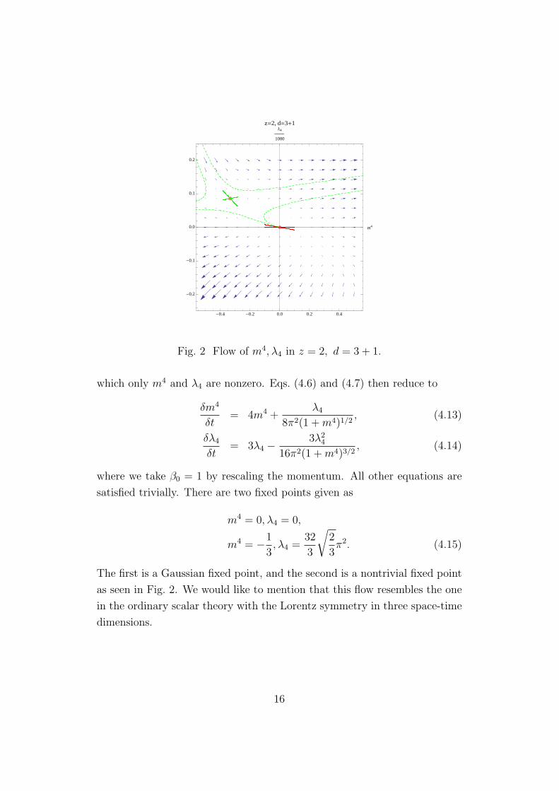
Fig. 2 Flow of m4, λ4 in z = 2, d = 3 + 1.

which only m4 and λ4 are nonzero. Eqs. (4.6) and (4.7) then reduce to

δm4

δt= 4m4 +

λ4

8π2(1 +m4)1/2, (4.13)

δλ4

δt= 3λ4 −

3λ24

16π2(1 +m4)3/2, (4.14)

where we take β0 = 1 by rescaling the momentum. All other equations are

satisfied trivially. There are two fixed points given as

m4 = 0, λ4 = 0,

m4 = −1

3, λ4 =

32

3

√2

3π2. (4.15)

The first is a Gaussian fixed point, and the second is a nontrivial fixed point

as seen in Fig. 2. We would like to mention that this flow resembles the one

in the ordinary scalar theory with the Lorentz symmetry in three space-time

dimensions.

16

4.2 Transformation of Variables

Our main interest is the restoration of the Lorentz symmetry in the IR region.

To discuss the RG flow in the IR region, it is useful to change the variable as

h =1

α0

, (4.16)

and introduce new variables with hats [20, 21, 23]

t = h−12 t, (4.17)

x = x, (4.18)

φ = h−14φ. (4.19)

The action in the model (4.1) with new variables is

S =

∫t,xi

1

2(∂0φ∂0φ+ ∂iφ∂iφ+ m2φ2)

+λ4

4!φ4 +

λ6

6!φ6 +

λ8

8!φ8 +

λ10

10!φ10

+1

2h∂i∂iφ∂j ∂jφ+

1

2

( α2

2!φ2∂iφ∂iφ+

α4

4!φ4∂iφ∂iφ

), (4.20)

where

m2 ≡ hm4, λ4 ≡ h32λ4, λ6 ≡ h2λ6, λ8 ≡ h

52λ8, λ10 ≡ h3λ10,

α2 ≡ h32α2, α4 ≡ h2α4, (4.21)

where we also take β0 = 1. The dimensions in the unit of mass of new

variables are as follows:

[t] = −1, [x] = −1, [φ] = 1, [m2] = 2, [λ4] = 0, [λ6] = −2,

[λ8] = −4, [λ10] = −6, [h] = −2, [α2] = −2, [α4] = −4. (4.22)

They are identical to the canonical dimension in the Lorentz theory in four

space-time dimensions.

The RG equations (4.4)–(4.12) in terms of the new variables (with hats)

are given as

δh

δt= −2h− α2h

8π2(1 + h+ m2)1/2, (4.23)

17

δm2

δt= 2m2 +

1

8π2(1 + h+ m2)1/2(α2 + λ4 − α2m

2), (4.24)

δλ4

δt= − 1

16π2(1 + h+ m2)3/23(α2 + λ4)

2

+1

16π2(1 + h+ m2)1/22(α4 + λ6)− 3λ4α2, (4.25)

δλ6

δt= −2λ6 +

1

32π2(1 + h+ m2)5/245(α2 + λ4)

3

− 1

16π2(1 + h+ m2)3/215(α2 + λ4)(α4 + λ6)

+1

8π2(1 + h+ m2)1/2(λ8 − 2λ6α2), (4.26)

δλ8

δt= −4λ8 −

1

64π2(1 + h+ m2)7/21575(α2 + λ4)

4

+1

16π2(1 + h+ m2)5/2315(α2 + λ4)

2(α4 + λ6)

− 1

16π2(1 + h+ m2)3/235(α4 + λ6)

2 + 28λ8(α2 + λ4)

+1

16π2(1 + h+ m2)1/2(2λ10 − 5α2λ8), (4.27)

δλ10

δt= −6λ10 +

1

128π2(1 + h+ m2)9/299225(α2 + λ4)

5

− 1

32π2(1 + h+ m2)7/223625(α2 + λ4)

3(α4 + λ6)

+1

32π2(1 + h+ m2)5/24725(α2 + λ4)(α4 + λ6)

2 + 1890(α2 + λ4)2λ8

− 1

16π2(1 + h+ m2)3/245λ10(α2 + λ4) + 210(α4 + λ6)λ8

− 3λ10α2

8π2(1 + h+ m2)1/2, (4.28)

δα2

δt= −2α2 −

1

48π2(1 + h+ m2)7/25(1 + 2h)2(α2 + λ4)

2

+1

32π2(1 + h+ m2)5/24α2(1 + 2h)(α2 + λ4) + (3 + 10h)(α2 + λ4)

2

− 1

48π2(1 + h+ m2)3/22α2

2 + 15α2(α2 + λ4)

18

-0.4 -0.2 0.0 0.2 0.4

-0.2

-0.1

0.0

0.1

0.2

m` 2

Λ`

4

10 000

d=3+1

Fig. 3 Flow of m2, λ4 in d = 3 + 1.

+1

16π2(1 + h+ m2)1/2(2α4 − 3α2

2), (4.29)

δα4

δt= −4α4 +

1

96π2(1 + h+ m2)9/2175(1 + 2h)2(α2 + λ4)

3

− 1

12π2(1 + h+ m2)7/230α2(1 + 2h)(α2 + λ4)

2 + 5(3 + 10h)(α2 + λ4)3

+5(1 + 2h)2(α2 + λ4)(α4 + λ6)

+1

32π2(1 + h+ m2)5/228α2

2(α2 + λ4) + 93α2(α2 + λ4)2

+4(3 + 10h)(α2 + λ4)(α4 + λ6) + 8(1 + 2h)(2α2α4 + α4λ4 + α2λ6)

− 1

48π2(1 + h+ m2)3/2(77α2α4 + 42α4λ4 + 27α2λ6)

− 1

4π2(1 + h+ m2)1/2(α2α4). (4.30)

If we set h = 0, α2 = 0, and α4 = 0, these RG equations exactly coincide

with the equations in the case of the local potential approximation in the

ordinary theory, which has Lorentz symmetry, as expected. As an example,

we give the RG flow in the theory subspace, in which only m2 and λ4 are

nonzero. (See Fig. 3.)

19

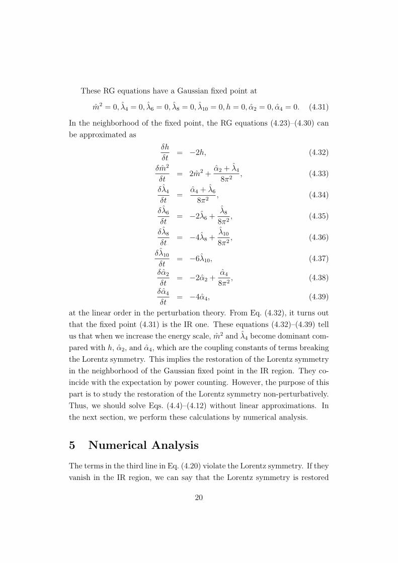
These RG equations have a Gaussian fixed point at

m2 = 0, λ4 = 0, λ6 = 0, λ8 = 0, λ10 = 0, h = 0, α2 = 0, α4 = 0. (4.31)

In the neighborhood of the fixed point, the RG equations (4.23)–(4.30) can

be approximated as

δh

δt= −2h, (4.32)

δm2

δt= 2m2 +

α2 + λ4

8π2, (4.33)

δλ4

δt=

α4 + λ6

8π2, (4.34)

δλ6

δt= −2λ6 +

λ8

8π2, (4.35)

δλ8

δt= −4λ8 +

λ10

8π2, (4.36)

δλ10

δt= −6λ10, (4.37)

δα2

δt= −2α2 +

α4

8π2, (4.38)

δα4

δt= −4α4, (4.39)

at the linear order in the perturbation theory. From Eq. (4.32), it turns out

that the fixed point (4.31) is the IR one. These equations (4.32)–(4.39) tell

us that when we increase the energy scale, m2 and λ4 become dominant com-

pared with h, α2, and α4, which are the coupling constants of terms breaking

the Lorentz symmetry. This implies the restoration of the Lorentz symmetry

in the neighborhood of the Gaussian fixed point in the IR region. They co-

incide with the expectation by power counting. However, the purpose of this

part is to study the restoration of the Lorentz symmetry non-perturbatively.

Thus, we should solve Eqs. (4.4)–(4.12) without linear approximations. In

the next section, we perform these calculations by numerical analysis.

5 Numerical Analysis

The terms in the third line in Eq. (4.20) violate the Lorentz symmetry. If they

vanish in the IR region, we can say that the Lorentz symmetry is restored

20

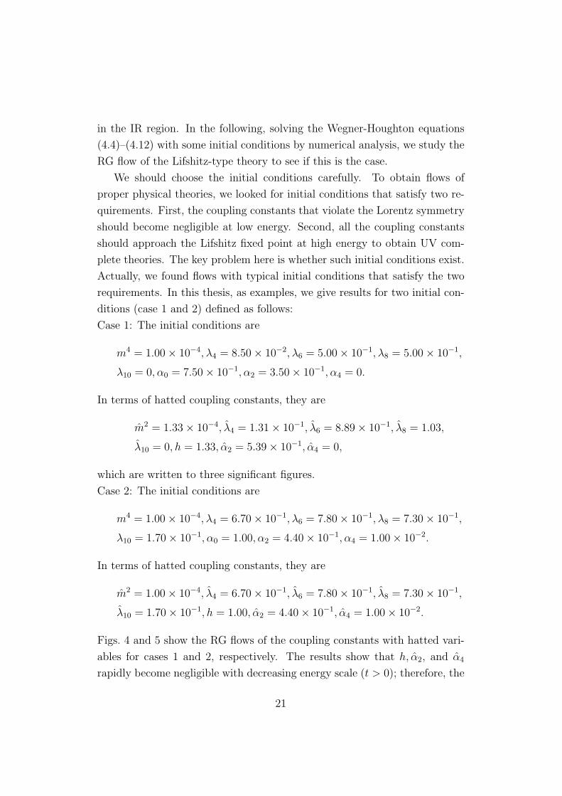
in the IR region. In the following, solving the Wegner-Houghton equations

(4.4)–(4.12) with some initial conditions by numerical analysis, we study the

RG flow of the Lifshitz-type theory to see if this is the case.

We should choose the initial conditions carefully. To obtain flows of

proper physical theories, we looked for initial conditions that satisfy two re-

quirements. First, the coupling constants that violate the Lorentz symmetry

should become negligible at low energy. Second, all the coupling constants

should approach the Lifshitz fixed point at high energy to obtain UV com-

plete theories. The key problem here is whether such initial conditions exist.

Actually, we found flows with typical initial conditions that satisfy the two

requirements. In this thesis, as examples, we give results for two initial con-

ditions (case 1 and 2) defined as follows:

Case 1: The initial conditions are

m4 = 1.00× 10−4, λ4 = 8.50× 10−2, λ6 = 5.00× 10−1, λ8 = 5.00× 10−1,

λ10 = 0, α0 = 7.50× 10−1, α2 = 3.50× 10−1, α4 = 0.

In terms of hatted coupling constants, they are

m2 = 1.33× 10−4, λ4 = 1.31× 10−1, λ6 = 8.89× 10−1, λ8 = 1.03,

λ10 = 0, h = 1.33, α2 = 5.39× 10−1, α4 = 0,

which are written to three significant figures.

Case 2: The initial conditions are

m4 = 1.00× 10−4, λ4 = 6.70× 10−1, λ6 = 7.80× 10−1, λ8 = 7.30× 10−1,

λ10 = 1.70× 10−1, α0 = 1.00, α2 = 4.40× 10−1, α4 = 1.00× 10−2.

In terms of hatted coupling constants, they are

m2 = 1.00× 10−4, λ4 = 6.70× 10−1, λ6 = 7.80× 10−1, λ8 = 7.30× 10−1,

λ10 = 1.70× 10−1, h = 1.00, α2 = 4.40× 10−1, α4 = 1.00× 10−2.

Figs. 4 and 5 show the RG flows of the coupling constants with hatted vari-

ables for cases 1 and 2, respectively. The results show that h, α2, and α4

rapidly become negligible with decreasing energy scale (t > 0); therefore, the

21

2 3 4 5t

0.2

0.4

0.6

0.8

1.0

g

€

ˆ m 2

€

ˆ α 4

€

ˆ λ 4

€

ˆ α 2

€

h

€

ˆ λ 8

€

ˆ λ 6

€

ˆ λ 10

Fig. 4 RG flow of hatted coupling constants against decreasing energy scale

t under the initial condition in case 1. The continuous lines show the flows

of the coupling constants h, α2, and α4, which violate the Lorentz symmetry.

The dashed lines show the ones of m2, λ4, λ6, λ8, and λ10.

2 3 4 5t

0.5

1.0

1.5

g

€

ˆ m 2

€

ˆ α 4

€

ˆ λ 4

€

ˆ α 2€

h

€

ˆ λ 8€

ˆ λ 6 €

ˆ λ 10

Fig. 5 RG flow of hatted coupling constants against decreasing energy scale

t under the initial condition in case 2.

third line terms of Eq. (4.20) turn out to be highly suppressed. This implies

that the Lorentz symmetry is restored in the IR region.

On the other hand, Figs. 6 and 7 show the RG flows of the unhatted

coupling constants with increasing energy scale (t < 0) for cases 1 and 2. The

results show that all the coupling constants approach the Lifshitz fixed point

with increasing energy. Therefore, we obtain the UV complete renormalizable

22

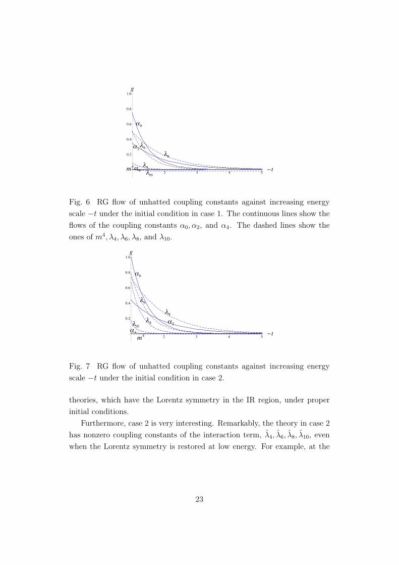
2 3 4 5t

0.2

0.4

0.6

0.8

1.0

g

€

m4

€

α4

€

λ4€

α2€

α0

€

λ8

€

λ6

€

λ10

Fig. 6 RG flow of unhatted coupling constants against increasing energy

scale −t under the initial condition in case 1. The continuous lines show the

flows of the coupling constants α0, α2, and α4. The dashed lines show the

ones of m4, λ4, λ6, λ8, and λ10.

2 3 4 5t

0.2

0.4

0.6

0.8

1.0

g

€

m4

€

α4

€

λ4

€

α2

€

α0

€

λ8

€

λ6

€

λ10

Fig. 7 RG flow of unhatted coupling constants against increasing energy

scale −t under the initial condition in case 2.

theories, which have the Lorentz symmetry in the IR region, under proper

initial conditions.

Furthermore, case 2 is very interesting. Remarkably, the theory in case 2

has nonzero coupling constants of the interaction term, λ4, λ6, λ8, λ10, even

when the Lorentz symmetry is restored at low energy. For example, at the

23

energy scale t = 3.5 in Fig. 5, the coupling constants are

m2 = 6.85× 10−1, λ4 = 6.55× 10−1, λ6 = 1.46× 10−2, λ8 = −3.06× 10−2,

λ10 = 2.46× 10−1, h = 6.72× 10−3, α2 = 3.01× 10−3, α4 = 2.45× 10−4,

which are written to three significant figures.

I would like to add comments about a fine-tuning of the initial conditions.

Actually, when we choose the initial conditions, it is not so hard to satisfy

the first requirement that the coupling constants that violate the Lorentz

symmetry should become negligible at low energy. To satisfy the second

requirement that all the coupling constants should approach the Lifshitz fixed

point at high energy, especially we carefully choose the initial conditions to

satisfy α4 = 0 and λ10 = 0. And because of the restriction owing to the

transformation of variables, we should satisfy the condition α0 > 0.

Finally, we would like to mention a possibility for other initial conditions.

It is possible that there are other interesting initial conditions, and to classify

the regions of the flows generally is an interesting future work. The most

important thing, however, is that there exists at least one such flow.

6 Short Summary

In the Lifshitz-type theory, higher derivative terms in the kinetic terms sup-

press the UV divergence. However, there is a problem of broken Lorentz sym-

metry; therefore, we should examine whether the theory restores the Lorentz

symmetry in the IR region. In this part, we applied the Wegner-Houghton

equation with the momentum cut-off in cylindrical shape and analyzed the

z = 2, d = 3 + 1 Lifshitz-type scalar model numerically. We find that the

terms that break the Lorentz symmetry vanish at low energy. Remarkably,

the Lifshitz-type theory has nontrivial interaction terms λnφn(n = 4, 6, 8, 10)

even when the Lorentz symmetry is restored at low energy. We find a concrete

solution to the long-standing problem of triviality of φ4 theory in d = 3 + 1.

In summary, z = 2, d = 3 + 1 Lifshitz-type scalar theory, at least for the

model in this thesis, restores the Lorentz symmetry in the IR region, and we

obtain a UV complete renormalizable theory under proper initial conditions.

24

The truncation method remains as a matter to be discussed further.

Given some symmetries, we may improve this analytic method. There is

also room for discussion on the cut-off method. In this part, we used the

cut-off to respect the spatial symmetry. More pertinent cut-off which keeps

the Lorentz symmetry explicitly may exist. It is interesting to challenge such

a problem. It would also be interesting to analyze multiple fields including

fermions. They are also soluble by this method in principle, although im-

provements may be needed in this analysis. If the theory can include the

gauge field, we could discuss the standard model. The gauge symmetry is

incompatible with the ERG, because a cut-off in the momentum space breaks

the symmetry explicitly. Therefore it is important to study a renormalization

method that keeps the gauge symmetry, which will be the subject of the next

part.

25

Part II

Gradient Flow Equation and

Its Supersymmetric Extension

The gauge symmetry guarantees the theoretical consistency such as the uni-

tarity and the renormalizability. However, some UV regularizations do not

respect the gauge symmetry. Momentum cut-off or Pauli-Villas regulariza-

tion are such examples. Since the ERG is formulated using a cut-off in a

momentum space, it breaks the gauge symmetry explicitly. How to analyze

the gauge theory using the ERG without breaking gauge symmetry explicitly

still remains an open problem. In this part, we discuss the method of the

gradient flow equation and its supersymmetric expansion. This discussion

would be important step towards the understanding the ERG which keeps

the symmetry explicitly.

7 Review of Gradient Flow Equation of Yang-

Mills Theory

Recently, Martin Luscher proposed an interesting method [2] to obtain renor-

malized physical quantities in an automatic fashion.

In this method, the expectation value in terms of new gauge field is finite

without additional renormalization. Here the new gauge field is constructed

by the solution of a certain type of diffusion equation called a gradient flow

equation, whose initial value is the bare gauge field. Luscher showed this at

one loop order as example [2], and later all order proof was given by Luscher

and Weisz [33]. We call the statement the Luscher-Weisz theorem. This

section is the review of Refs. [2, 6, 33].

26

7.1 Definition of Gradient Flow Equation

The gauge field Bµ is defined by the gradient flow

Bµ = DνGνµ + α0Dµ∂νBν , (7.1)

Bµ|t=0 = Aµ. (7.2)

where the dot means a differential in terms of the flow time t, Aµ describe a

fundamental bare field of SU(N) gauge theory, Gµν and Dµ are defined by

Gµν = ∂µBν − ∂νBµ + [Bµ, Bν ], (7.3)

Dµ = ∂µ + [Bµ, ·] (7.4)

respectively. The reason why we call the equation the gradient flow one is

that the first term of R.H.S. of Eq. (7.1) is proportional to the gradient of

the action,

S =

∫dDxTr[Gµν(x)Gµν(x)]. (7.5)

The second term of the R.H.S. of Eq. (7.1) is the gauge fixing term over

the flow time direction. The term is introduced to cause suppression of the

increase of the degree of new gauge freedom over the direction. In this thesis,

we call this term the α0 term to avoid needless confusion with the usual gauge

fixing term in the Yang-Mills theory.

7.2 Luscher-Weisz Theorem

Luscher claims that any expectation value which is described by the gauge

filed B, which is defined by Eq. (7.1) at positive flow time has a well-defined

continuum limit without additional renormalization. Calculating the expec-

tation value of the energy density at one loop order using this method, he

showed that it is the case [2]. Soon after that, Luscher and Weisz proved this

claim to all order in perturbation theory [33].

27

Luscher-Weisz Theorem In the Yang-Mills theory, the expectation value in terms of the new gauge

field, which is defined by the solution of the gradient flow equation, are

finite without additional renormalization to all loop order, once the the-

ory in terms of the fundamental gauge field is renormalized in the usual

way. There are various applications owing to the theorem as we shall explain

later in Sec. 7.4. The detailed proof of the theorem is given in Ref. [33], and

we briefly summarize the points of the proof of the theorem as a review. The

proof of the theorem consists of six steps:

1. The theory is reformulated as the field theory in 4+1 dimensions which

represent the space coordinate xµ and the flow time t.

2. The flow equation is realized by introducing the flow action Sfl in 4+1

dimensions with the Lagrange-multiplier field Lµ(t, x).

Sfl = −2

∫ ∞

0

dt

∫d4xtrLµ(t, x)(∂tBµ −DνGνµ − α0Dµ∂νBν)(t, x). (7.6)

Thus the gradient flow equation is described by the local field theory.

3. If the interactions are local, the divergent part can be canceled by

local counterterm which can be localized either in the bulk or at the

boundary, that is, the divergent part can be localized in the bulk or at

the boundary of the half space.

4. Since the theory has no loop diagrams in the bulk, there are no diver-

gences in the bulk. Therefore divergences are localized at the boundary,

if they exist.

5. Since there are divergences only in the term which involves bulk field

on the boundary, the divergence terms are proportional to Lµ and d.

Here d is an additional ghost field which lives in D + 1 dimensions.

Owing to the Lorentz symmetry, the BRS symmetry, the ghost num-

ber conservation and the dimensional analysis, the possible boundary

28

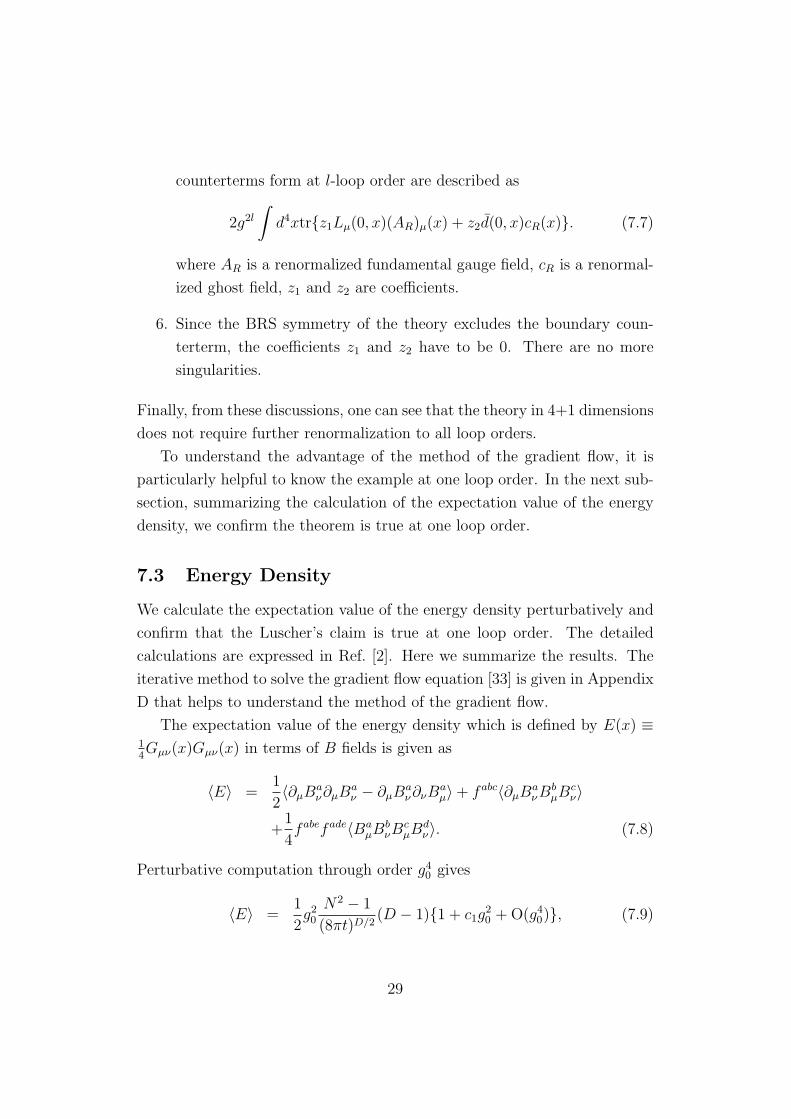
counterterms form at l-loop order are described as

2g2l

∫d4xtrz1Lµ(0, x)(AR)µ(x) + z2d(0, x)cR(x). (7.7)

where AR is a renormalized fundamental gauge field, cR is a renormal-

ized ghost field, z1 and z2 are coefficients.

6. Since the BRS symmetry of the theory excludes the boundary coun-

terterm, the coefficients z1 and z2 have to be 0. There are no more

singularities.

Finally, from these discussions, one can see that the theory in 4+1 dimensions

does not require further renormalization to all loop orders.

To understand the advantage of the method of the gradient flow, it is

particularly helpful to know the example at one loop order. In the next sub-

section, summarizing the calculation of the expectation value of the energy

density, we confirm the theorem is true at one loop order.

7.3 Energy Density

We calculate the expectation value of the energy density perturbatively and

confirm that the Luscher’s claim is true at one loop order. The detailed

calculations are expressed in Ref. [2]. Here we summarize the results. The

iterative method to solve the gradient flow equation [33] is given in Appendix

D that helps to understand the method of the gradient flow.

The expectation value of the energy density which is defined by E(x) ≡14Gµν(x)Gµν(x) in terms of B fields is given as

〈E〉 =1

2〈∂µB

aν∂µB

aν − ∂µB

aν∂νB

aµ〉+ fabc〈∂µB

aνB

bµB

cν〉

+1

4fabefade〈Ba

µBbνB

cµB

dν〉. (7.8)

Perturbative computation through order g40 gives

〈E〉 =1

2g20

N2 − 1

(8πt)D/2(D − 1)1 + c1g

20 + O(g4

0), (7.9)

29

where

c1 =(4π)ε(8t)ε

16π2

N

(11

3ε+

52

9− 3 ln 3

)−Nf

(2

3ε+

4

9− 4

3ln 2

)+ O(ε)

. (7.10)

On the other hand, the bare coupling g0 is related to the renormalized

coupling g in the MS scheme at scale µ as

g20 = g2µ2ε(4πe−γE)−ε

1− 1

εb0g

2 + O(g4)

, (7.11)

where

b0 =1

16π2

11

3N − 2

3Nf

. (7.12)

Substituting (7.11) into (7.9), we obtain

〈E〉 =3(N2 − 1)g2

128π2t21 + c1g

2 + O(g4). (7.13)

Here

c1 =1

16π2

N

(11

3L+

52

9− 3 ln 3

)−Nf

(2

3L+

4

9− 4

3ln 2

)(7.14)

at ε = 0 with L = ln 8µ2t + γE. Thus one can see that the energy density

defined in terms of B field is finite without additional renormalization.

7.4 Applications of Gradient Flow Equation

Various applications of the physical observable are studied recently. We

introduce some of them as example. This subsection is a review of Ref. [6].

7.4.1 Chiral Condensate

In lattice QCD, the expectation value of the chiral densities

Srst ± P rs

t , r, s ∈ u, d (7.15)

where Srst = χrχs, P

rst = χrγ5χs, the r and s are flavor labels, is the order

parameter for the spontaneous breaking of the chiral symmetry. The bare

operators contain the UV divergences. When the lattice theory has a chiral

30

symmetry, this divergent terms are proportional to the light-quark masses.

Because of the arbitrariness of the subtraction for the renormalization, the

expectation value loses the meaning as the order parameter.

Luscher proposed that the gradient flow of a matter field [6] is

χ = ∆χ, χ|t=0 = ψ (7.16)

∆ = /D2 or simply ∆ = DµDµ, (7.17)

where Dµ = ∂µ +Bµ. Using this equation, he calculates the flow time depen-

dent chiral condensate. Because Eq. (7.16) has chiral symmetry, the quark

field χ(t, x) which depends on flow time transforms in the same way as the

fundamental quark field ψ(x) under global chiral rotations. He defines the

time dependent condensate as

Σt = −1

2

⟨Suu

t + Sddt

⟩, (7.18)

Σt is also an order parameter for the spontaneous breaking of chiral symme-

try. The attractive point is that Σt does not have power divergence, so there

are no arbitrariness in the subtraction. There are also advantages that the

calculation of Σt through numerical simulation is straightforward.

7.4.2 Small Flow Time Expansion

The method to use the gradient flow equation has the advantage that there

are no divergence at flow time t > 0. It is also important to study how

exactly the divergence are avoided near the boundary. Through the small

flow time expansion, we can examine them. We can describe the asymptotic

expansion of gauge invariant local fields Ot(x) in respect to φk(x) which is

the field on the boundary as

Ot(x) ∼t→0

∑k

ck(t)φk(x), (7.19)

where ck(t) is a time dependent coefficient. The coefficients satisfy the RG

equation which determines the asymptotic behavior at small flow time as

ck(t) ∝t→0

t12(dk−d0)gνk1 + O(g2), (7.20)

31

where dk and d0 are dimensions of φk(x) and Ot(x) respectively, g is a run-

ning coupling of the theory, νk is determined by the one loop coefficients of

their anomalous dimensions. Judging from (7.20), the expansion of Ot(x)

of Eq. (7.19) is dominated by φk(x) with the lowest dimension in the limit

t → 0. For example, the chiral densities (7.15) can be described using the

expansion (7.19). The details are explained in Ref. [6] and their references.

In an opposite manner, any gauge invariant local field φ(x) at the bound-

ary is also expanded in respect to Ot(x) at some positive flow time t. The

simplest case is that we restrict the field by their dimension and symmetry.

The form is represented as

φ(x) = c(t)Ot(x) +O(t). (7.21)

It is important work to determine the coefficient c(t). For example, in

Refs. [15] the coefficient in the expansion of the energy-momentum tensor

in the pure gauge theory is computed at one loop order perturbatively. Also,

in the paper, using the method of the gradient flow equation, the relation

between the small flow time behavior of certain gauge invariant local prod-

ucts and the correctly-normalized conserved energy-momentum tensor in the

Yang-Mills theory is given. In Refs. [8], using the Ward identities that de-

rive from the conservation of the energy-momentum tensor in the continuum

theory, the coefficients is determined non-perturbatively. In the paper, they

also use the gradient flow in order to define more appropriate probes for the

translation Ward identities.

7.4.3 Step Scaling and Improved Action

Since the gradient flow gives UV finite quantity, one can define a new renor-

malization scheme for the running coupling constant. In Refs. [2, 9, 10,

11, 12, 13], the running coupling constant is defined by the renormalization

condition:

g2(L) = constant× t2 〈Et〉√8t= 13L. (7.22)

Using the step scaling, the RG evolution of this running coupling constant

can be studied non-perturbatively.

32

On the other hand, the method of the gradient flow is useful to construct

improved actions. The parameter of the improved theory can be tuned by

matching lattices with different spacings using sufficient number of observ-

ables as inputs. Since there are a lot of candidates of observables such as

trGµνGµν, χχ, χσµνGµνχ, (χΓχ)(χΓχ), (7.23)

the method of the gradient flow is very useful.

8 Supersymmetric Gradient Flow Equation

As we have seen in the previous section, the gradient flow equation has

spurred a great deal of research. There are a lot of applications using this

new renormalization, but there is also room for theoretical study. One of

them is to find out what physical system this method can be applied. The

equation is very attractive, therefore it is worth extending the equation to

other theory, for example, to the QCD with matter field. Luscher proposed

the gradient flow of the matter field as Eq. (7.16). However the quark part of

this equation is no longer defined from the gradient of the action and there

is an arbitrariness of ∆ as in Eq. (7.17). It would be important to study the

theoretical basis how to defined the gradient flow equation with matter fields

in the gauge theory. One of the interesting systems is the super Yang-Mills

theory. This theory has a gaugino, which is a matter field in the adjoint

representation. And the gaugino is closely related to the gauge fields by

supersymmetry (SUSY). Therefore we study the supersymmetric extension

of the gradient flow equation. Since the supersymmetric Yang-Mills theory

is an attractive of its own sake, it would be useful to study the gradient

flow equation for this system. It may also give us a hint to understand the

theoretical basis of the gradient flow equation including matter fields.

We give a short summary of SUSY in Appendix E as a review of Ref. [34].

33

8.1 Our Proposal for Supersymmetric Gradient Flow

Equation

The purpose of this subsection is to explain our proposal for the gradient

flow equation in super Yang-Mills theory. We success the expansion of the

gradient flow equation to super Yang-Mills theory. At first, we summarize

how to derive the gradient flow in Yang-Mills theory as follows:

1. Starting from the Yang-Mills action SYM, we make a variation over the

Aµ(x) field.

2. We replace the Aµ(x) field with the new gauge fieldBµ(t, x), and impose

the initial condition Bµ(0, x) = Aµ(x)

3. We add a new gauge fixing term to suppress the increase of the degree

of new gauge freedom in the flow time direction. It has to be propor-

tional to the gauge transformation, because physical quantities does

not depend on the term.

4. We regard the sum of them as R.H.S. of the gradient flow equation.

5. We regard the derivative of Bµ(t, x) with respect to t as L.H.S. of the

gradient flow equation.

Thus, we obtain the gradient flow equation in Yang-Mills theory as Eqs. (7.1)

and (7.2).

To obtain the gradient flow equation to super Yang-Mills theory, we re-

place the statement partly as follows:

• Yang-Mills action SYM → Super Yang-Mills action SSYM.

• Gauge field Aµ(x) → Superfield V .

• New gauge field Bµ(t, x) → New superfield v.

• Gauge transformation → Super gauge transformation.

Thus we propose a general form of the supersymmetric extension of the

gradient flow equation.

34

Supersymmetric Gradient Flow Equation ∂va

∂t=δSSYM

δva+ α0δva. (8.1)

where V = vaTa and T a is a representation matrix. Because Eq. (8.1),

however, have infinite number of terms, it is very difficult to solve it non-

perturbatively. In order to obtain the flow equation with finite number of

terms, we choose the Wess-Zumino (WZ) gauge. However, generally the time

evolution from the flow equation can carry the system away from the WZ

gauge. Therefore, the most important question is whether there exists the

special α0 term, which keeps the WZ gauge. As a result, we find that such a

α0 term exists:

Supersymmetric Gradient Flow Equation under Wess-Zumino Gauge ∂v

∂t=eLv − 1

Lv

· (Dαwα + e−vDαev, wα) + h. c.+ δv, (8.2)

where

δv = φ+ φ† +1

2[v, φ− φ†] +

1

12[v, [v, φ+ φ†]], (8.3)

φ = D2(D2v + [D2v, v]). (8.4) Using this new equation, we find out that, in this case, an extra term is

required in addition to the gradient flow equation of the matter field which

is proposed by Luscher.

9 Pure Abelian Supersymmetric Theory

At first, we consider a supersymmetric pure Abelian gauge theory to simplify

the discussion. Because this theory does not have an interaction, the theory

also does not have divergences in the first place, but it is useful to understand

the basic structure as a toy model.

35

9.1 Derivation of Gradient Flow Equation of Pure Abelian

Supersymmetric Theory

From the discussion in Sec. 8.1, we obtain the gradient flow Equation of the

pure Abelian supersymmetric theory. The free vector field action which is

invariant under the supersymmetric gauge transformation is

S =1

4

∫d4x(WαWα|θθ + WαW

α|θθ)

=1

4

∫d8z(DαWα + DαW

α)V (9.1)

where V is vector multiplet, V = C,X, X,M,M∗, Vm,Λ, Λ, D. W and W

are defined by

Wα = −DDDαV, (9.2)

Wα = −DDDαV. (9.3)

Making variation of the action S over V , we obtain

δS

δV= DαWα. (9.4)

We used here the relation equation,

DαWα = DαWα. (9.5)

Then we proposed the extended gradient flow equation of the pure super-

symmetric theory as

v = Dαwα + α0(D2D2 + D2D2)v, (9.6)

v|t=0 = V, wα|t=0 = Wα. (9.7)

where v is vector multiplet depending on the flow time, v = c, χ, χ,m,m∗, vm, λ, λ, d.The α0 term, which is the second term of the R.H.S. of Eq. (9.6), is intro-

duced to suppress the new gauge degrees of freedom under the evolution in

the flow time. The α0 term may not be unique, but we here only show that

the form Eq. (9.6) is adequate. We postpone to explain how to determine

the α0 term to Sec. 10.2.2.

36

9.2 Gradient Flow Equation of Pure Yang-Mills The-

ory for Each Component of Vector Multiplet

Describing the extended gradient flow equation in the coordinate of super-

space which are labeled (x, θ, θ), we find out the each dependence of the

component of vector multiplet on the flow time.

v(x, θ, θ) = c+ iθχ− iθχ+i

2θθm− i

2θθm∗

−θσmθvm + iθθθ[λ+i

2σm∂mχ]

−iθθθ[λ+i

2σm∂mχ] +

1

2θθθθ[d+

1

2c] (9.8)

Using (9.8), we calculate each terms of the gradient flow equation, we obtain

Dαwα = −2d+ 2θσm∂mλ− 2θσm∂mλ+ 2(θσkθ)∂mvkm

−iθθθλ+ iθθθλ+1

2θθθθd, (9.9)

(D2D2 + D2D2)v = 16(d+ c)− 16θ(σm∂mλ− iχ) + 16θ(σm∂mλ− iχ)

+8iθθm− 8iθθm∗ − 16(θσmθ)∂m∂kvk

+8iθθθ(λ+ iσm∂mχ)− 8iθθθ(λ+ iσm∂mχ)

+4θθθθ(d+ c). (9.10)

Substituting (9.9) and (9.10) into (9.6), finally, we obtain the flow equations

for the each component of the vector multiplet as

c = 16α0c− 2(1− 8α0)d, (9.11)

χ = 16α0χ− 2i(1− 8α0)σm∂mλ, (9.12)

˙χ = 16α0χ− 2i(1− 8α0)σm∂mλ, (9.13)

m = 16α0m, (9.14)

m∗ = 16α0m∗, (9.15)

vm = 2vm − 2(1− 8α0)∂m∂kvk, (9.16)

˙λ = 2λ, (9.17)

λ = 2λ, (9.18)

d = 2d. (9.19)

37

Taking α0 as

α0 =1

8, (9.20)

we obtain

c = 2c, (9.21)

χ = 2χ, (9.22)

˙χ = 2χ, (9.23)

m = 2m, (9.24)

m∗ = 2m∗, (9.25)

vm = 2vm, (9.26)

˙λ = 2λ, (9.27)

λ = 2λ, (9.28)

d = 2d. (9.29)

One can see that each component of the vector multiplet evolves separately

in time.

9.3 Flow Time Dependence of Super Gauge Transfor-

mation

When we demand that the gradient flow equation (9.6) is invariant under

the super gauge transformation,

v′ = v + φ+ φ†, (9.30)

at each time, φ have to satisfy the equation as

φ = α0D2D2φ, (9.31)

φ|t=0 = Φ, (9.32)

where Φ is a chiral field,

DΦ = 0. (9.33)

The chirality of the φ at each flow time is guaranteed by Eq. (9.31).

38

10 Super Yang-Mills Theory

Following the toy model example in Sec. 9, we extend the gradient flow

equation to the case of super Yang-Mills theory. In the general gauge, the

flow equation contains infinite number of commutators so that it is very

difficult to solve it non-perturbatively. In order to obtain the flow equation

with finite number of terms, we choose the WZ gauge. However, generally

the time evolution from the flow equation can carry the system away from the

WZ gauge. Therefore, the most important question is whether there exists

a special α0 term, which keeps the WZ gauge. As a result, we find that such

a α0 term exists.

10.1 Derivation of Gradient Flow Equation for Super

Yang-Mills Theory

The gradient flow for super Yang-Mills theory is similar to the one for pure

Abelian supersymmetric theory in Sec. 9. The gauge fixing term is positive

and described by super gauge transformation δv. Then the most general

form of the supersymmetric gradient flow equation is

∂va

∂t=δSSYM

δva+ α0δva. (10.1)

In what follows we call the first term of R.H.S. as the gauge covariant term,

the second term of R.H.S. as the α0 term.

At first, we derive the gauge covariant term of the super Yang-Mills the-

ory. The action of the super Yang-Mills theory is

S =

∫d4xTr[WαWα|θθ + WαW

α|θθ]. (10.2)

The action is rewritten as

S =

∫d8zTr[Wαe−VDαe

V ] + h.c., (10.3)

where d8z ≡ d4xd2θd2θ, δva(z)δvb(z′)

≡ δab δ

8(z−z′) ≡ δab δ

4(x−x′)δ2(θ−θ′)δ2(θ− θ′).Wα is defined as

Wα = −D2(e−VDαeV ). (10.4)

39

The variation of S over V is

δS

δV≡

∑a

T a δS

δva(10.5)

=eLV − 1

LV

· (DαWα + e−VDαeV ,Wα) + h.c., (10.6)

where

LV · ≡ [V, · ]. (10.7)

The detailed derivation of Eq. (10.6) is given in Appendix F. In the next step,

we would like to determine the form of the α0 term. As mentioned above,

however, the gradient flow equation contains infinite number of commutators

in the general gauge. In order to obtain the flow equation with finite number

of terms, we choose the WZ gauge.

10.2 Gradient Flow Equation in Super Yang-Mills The-

ory under Wess-Zumino Gauge

In this subsection, we determine the form of the gradient flow equation for

super Yang-Mills theory under the WZ gauge .

10.2.1 Determination of Gauge Covariant Term

We define A as

A = Dαwα + e−vDαev, wα, (10.8)

Useful formulae expand Eq. (10.8) in component fields are given in Appendix

G. The gauge covariant term is given as(eLv − 1

Lv

· A)

+

(eLv − 1

Lv

· A)†

= A+ A† +1

2![v,A− A†] +

1

3![v, [v, A+ A†]] +O(v3), (10.9)

40

where A is represented in (x, θ, θ) coordinates by

A(x, θ, θ) = −8d+ 8θσmDmλ− 8θσmDmλ

+4(θσmθ)[vm, d] + 4(θσkσmσlθ)Dlvmk + 8[θλ, θλ]

−8iθθ(θσlσmDlDmλ) + 8iθθ[θλ, d]

+4iθθ(θσkσm∂kDmλ) + 4iθθ(θσkσm∂kDmλ)

+θθθθ(2d+ 2i∂m[vm, d] + iTr[σmσlσnσk]∂nDlvmk

−2i∂mλα, (σmλ)α

).

(10.10)

On the other hand, A† is represented in (x, θ, θ) coordinates by

A†(x, θ, θ) = −8d+ 8θσmDmλ− 8θσmDmλ

−4(θσmθ)[vm, d] + 4(θσlσmσkθ)Dlvmk + 8[θλ, θλ]

−4iθθ(θσkσm∂kDmλ)− 4iθθ(θσkσm∂kDmλ)

+8iθθ(θσlσmDlDmλ) + 8iθθ[θλ, d]

+θθθθ(2d+ 2i∂m[vm, d]− iTr[σmσkσnσl]∂nDlvmk

+2i∂m(λσm)α, λα).

(10.11)

Finally, we get the gauge covariant term in (x, θ, θ) coordinates as follows.(eLv − 1

Lv

·(Dαwα + e−vDαev

))+ h.c.

= −16d+ 16θσmDmλ− 16θσmDmλ

+16θσmθDkvmk + 16[θλ, θλ]

−8iθθ(θσlσmDlDmλ) + 8iθθ[θλ, d]

+8iθθ(θσlσmDlDmλ) + 8iθθ[θλ, d]

+θθθθ(4d+ 4i∂m[vm, d]

+iTr[σmσlσnσk − σmσkσnσl]DnDlvmk

−2i∂mλα, (σmλ)α+ 2i∂m(λσm)α, λα

−2

3[vm, [v

m, d]]). (10.12)

41

10.2.2 Determination of α0 Term

As mentioned above, we need to add the α0 term with (10.12) to suppress the

gauge degrees of freedom under the flow time evolution. Here we discuss how

to determine the form of the α0 term. The gauge transformation is defined

by

δV = LV/2 · [(Φ− Φ†) + coth (LV/2) · (Φ + Φ†)], (10.13)

where Φ and Φ† are a chiral superfield and an anti-chiral superfield respec-

tively. Under the WZ gauge, the gauge transformation is expressed by a

finite number of terms as

δV = Φ + Φ† +1

2[V,Φ− Φ†] +

1

12[V, [V,Φ + Φ†]]. (10.14)

We try to find out the special form of the α0 term so that the gradient flow

equation is consistent within the WZ gauge. This means the α0 term has to

satisfy the following requirements.

• It is positive.

• The mass dimension is two.

• It is described by super gauge transformation δV .

• The flow of the vector field keeps the WZ gauge at any flow time.

As a result, we found out that there exists at least one example of the α0

term which satisfies these conditions. The form is δV , which consists of Φ

defined by

Φ = D2(D2V + [D2V, V ]). (10.15)

42

Using this, we obtain δv in terms of (x, θ, θ) coordinates as

δv(x, θ, θ) = φ+ φ† +1

2[v, φ− φ†] +

1

12[v, [v, φ+ φ†]]

= 16d− 16θσmDmλ+ 16θσmDmλ− 16θσkθDk∂mvm

−8iθθθσkσmDkDmλ− 8θθθα[λα, ∂mvm]

−8iθθθσkσmDkDmλ− 8θθθα[λα, ∂mvm]

+4θθθθ(d+ iλα, (σ

mDmλ)α − iλα, (σmDmλ)α

+i[d, ∂mvm] + i[vm, ∂md]−

1

6[vm, [v

m, d]]). (10.16)

10.3 Gradient Flow Equation of Super Yang-Mills The-

ory for Each Component of Vector Multiplet

We substitute (10.12) and (10.16) into (10.1) under the WZ gauge. Because

a physical quantity does not depend on the form of the α0 term, we choose

a particular value α0 = 1. Then we obtain(eLv − 1

Lv

·(Dαwα + e−vDαev, wα

))+ h.c.+ 1 · δv

= 16θσmθDkvmk + 16[θλ, θλ]− 16θσkθDk∂mvm

−16iθθθσkσmDkDmλ+ 8iθθ[θλ, d+ i∂mvm]

+16iθθθσkσmDkDmλ+ 8iθθ[θλ, d− i∂mvm]

+θθθθ(8d+ 8i[vm, ∂

md] + iTr[σmσlσnσk − σmσkσnσl]DnDlvmk

+4iλα, (σmDmλ)α − 4iλα, (σmDmλ)α −

4

3[vm, [v

m, d]]). (10.17)

Finally, we obtain the flow equations for the each component of the vector

multiplet as

c = 0, (10.18)

χ = 0, (10.19)

˙χ = 0, (10.20)

m = 0, (10.21)

m∗ = 0, (10.22)

vm = −16Dkvmk + 16Dm∂kvk − 8λα, (σmλ)α, (10.23)

43

˙λ = −16σkσmDkDmλ+ 8[λ, d+ i∂mvm], (10.24)

λ = −16σkσmDkDmλ− 8[λ, d− i∂mvm], (10.25)

d = 16d+ 16i[vm, ∂md]

+2iTr[σmσlσnσk − σmσkσnσl]DnDlvmk

+8iλα, (σmDmλ)α − 8iλα, (σmDmλ)α

−8

3[vm, [v

m, d]]. (10.26)

We find that the flow equations for each component are consistent with WZ

gauge. Here we choose initial conditions to satisfy the WZ gauge at t = 0 as

c|t=0 = 0, (10.27)

χ|t=0 = 0, (10.28)

χ|t=0 = 0, (10.29)

m|t=0 = 0, (10.30)

m∗|t=0 = 0, (10.31)

vm|t=0 = Vm, (10.32)

λ|t=0 = Λ, (10.33)

λ|t=0 = Λ, (10.34)

d|t=0 = D. (10.35)

Let us compare the flow equation for Yang-Mills theory proposed by Luscher

with our results for super Yang-Mills theory in Eqs (10.24) and (10.25). In

Ref. [7], Luscher claims that the gradient flow equations of the quark field

are given as

˙χ = χ←−∆ + α0χ∂νBν , (10.36)

χ = ∆χ− α0∂νBνχ. (10.37)

On the other hand our results for the gradient flow equations of the gaugino

field in Eqs. (10.24) and (10.25) are given as

˙λ = −16σkσmDkDmλ+ 8[λ, d+ i∂mvm], (10.38)

λ = −16σkσmDkDmλ− 8[λ, d− i∂mvm]. (10.39)

44

We find that if we regard ∆ as /D2, Eqs. (10.36) and (10.37) are almost similar

to our results Eqs. (10.38) and (10.39) respectively except for [λ, d] term and

[λ, d] term and the point that α0 terms are described in terms of commutation

relations.

11 Short Summary

We proposed a supersymmetric extension of the gradient flow equation using

the superfield formalism. Since in the general gauge the equation involves

infinite number of terms, it is difficult to solve it non-perturbatively. In order

to obtain the gradient flow equation with finite number of terms, we need to

take the WZ gauge. We find a special form of the α0 term so that the gradient

flow equation is consistent within the WZ gauge. Since the super Yang-Mills

theory has a gaugino which is closely related to the gauge fields by SUSY,

the gradient flow in the super Yang-Mills theory leads to the equation of the

matter field. It is important to examine whether gauge invariant physical

quantities require additional renormalization or not, which is under way.

I would like to add comments as follows. There is not an explicit reason

why we have to derive the gradient flow equation by the gradient of the

action. If the theory has SUSY, there is an explicit relation between the

gradient flow equation of the gauge field and the one of the matter field.

In this work, we show that we can construct the each equation consistently

under the WZ gauge. However it is valid to derive the gradient flow equation

from the gradient of the action, when we study the correspondence between

the ERG equation and the gradient flow equation. The scale which is the

limit of the low energy corresponds to the flow time when the gradient of the

action equals 0, that is, the equation of motion is valid.

When we extend the gradient flow equation to the supersymmetric one,

we could derive the equation of the matter field naturally. In other words,

owing to the SUSY transformation, which gives the relation between the

gauge field and the gaugino field, we can obtain the consistent method to

construct the flow equations. Using the method, there is no arbitrariness of

the form of the flow equation of the matter fields.

We used the superfield formalism to extend the gradient flow equation

45

for the super Yang-Mills theory, but we can also use the supermultiplet for-

malism. Using the formalism, it is useful to extend for N = 2 SUSY. This is

the futures work.

46

12 Summary and Disucussion

In this thesis, we study new directions in the ERG through the Lifshitz-type

theory, the gradient flow equation and its supersymmetric extension.

In the Lifshitz-type theory, higher derivative terms in the kinetic terms

suppress the UV divergence. However, there is a problem of broken Lorentz

symmetry, therefore, we should examine whether the theory restores the

Lorentz symmetry in the IR region.

In part I, we applied the Wegner-Houghton equation with the momentum

cut-off in the cylindrical shape and analyzed the RG flow in the z = 2,

d = 3+1 Lifshitz-type scalar model numerically. As a result, we find that the

terms that break the Lorentz symmetry vanish at low energy for the Lifshitz-

type scalar model. There are two significances in the results. First, Lifshitz-

type theory has the advantage in terms of the renormalization. Since we

found the restoration of Lorentz symmetry, the theory broadens the class of

perturbatively renormalizable field theories which can be applied to particle

physics. Secondly, it means that this is a concrete solution to the problem

of triviality of φ4. The Lifshitz-type theory has nontrivial interaction terms

λnφn(n = 4, 6, 8, 10) even when the Lorentz symmetry is restored at low

energy. We find a concrete solution to the long-standing problem of triviality

of φ4 theory in d = 3 + 1.

There is also room for discussion on the cut-off method. We used the

cut-off to respect the spatial symmetry. More pertinent cut-off which keeps

the symmetry explicitly may exist. The truncation method remains as a

matter to be discussed further. Given some symmetries, for example SUSY,

we may improve this analytic method. If the theory can include the gauge

field, we could discuss the standard model, then we could extend the range

of application of Lifshitz-type theory further. For this purpose, the ERG

for supersymmetric theory and the gauge theory should be studied, that is

to say, we should study the cut-off problem which means how to keep the

symmetry explicitly of the cut-off in the ERG.

On the other hand, the gradient flow equation is also an attractive method

in terms of the renormalization. In this method, the expectation value of any

gauge invariant local operators constructed by the solution of a certain type

47

of diffusion equation called the gradient flow equation whose initial value

is the bare gauge field, is finite without additional renormalization. It is

interesting to find out in what physical system this method can be applied.

In part II, we give the general form of the supersymmetric extended gradi-

ent flow equation. However, since the equation has infinite number of terms,

it is difficult to solve it non-perturbatively. In order to obtain the gradient

flow equation with finite number of terms, we need to take the WZ gauge.

We find that we can obtain a consistent gradient flow equation within the

WZ gauge, if we choose a proper α0 term, which is described in terms of Φ

defined by Eq. (10.15). As a result, we give the gradient flow equation to the

super Yang-Mills theory which is closed under the WZ gauge.

There are two significances in our result. First, we extend the method of

the gradient flow equation to one of the super Yang-Mills theory. Since the

super Yang-Mills theory is attractive for its own sake, the gradient flow equa-

tion will be useful for further studies. Secondly, we obtain the gradient flow

equation of the matter field very naturally. Luscher proposed the gradient

flow of the matter field. However the quark part of this equation is no longer

defined from the gradient of the action, therefore there is an arbitrariness.

Since the super Yang-Mills theory has a gaugino which is closely related to

the gauge fields by SUSY, the gradient flow in the super Yang-Mills theory

leads the equation of the matter field.

Of course it is also important to study whether the physical quantities do

not require additional renormalization. This theory may be applied to the

ERG equation, which keeps the gauge symmetry. Moreover if we formulate

the equation, which is SUSY invariant at each flow time, it may lead to

construct the ERG equation, which keeps the SUSY explicitly. In either

case, the gradient flow equation is maybe a key to find a new ERG.

In conclusion, our results is not only attractive itself but also give the

new direction in the ERG to keep the symmetry explicitly. We hope that

our results in this thesis could give a first step towards the study on the new

ERG.

48

Acknowledgments

Before anything else, we would like to thank PhD supervisor, Prof. Tet-

suya Onogi for very stimulating discussion, meaningful advice, encourage-

ments and many lecture throughout this thesis. We also would like to thank

Prof. Kiyoshi Higashijima and Etsuko Itou. The work in Part I could not be

accomplished without their great advising. Owing to Prof. Martin Luscher’s

great work, we could achieve our work. Prof. Martin Luscher is so kind

to tell us detailed calculations. We would like to express our appreciation

to him. We also thank Prof. Satoshi Yamaguchi for many useful comments.

We acknowledge all our laboratory members for joyful discussions. This work

was supported by Grant-in-Aid for JSPS Fellows Grant Number 25·1336.

Finally we would like to thank my parents, my brother, specially my

fiancee for continuous encouragements.

49

A Notation in Part. I

We use the following notation. The definitions of integral symbols are∫x

≡∫ddx, (A.1)∫

p

≡∫

ddp

(2π)d. (A.2)

The definitions of δ functions and its symbols are∫x

δ(x)g(x) = g(0), (A.3)∫p

δ(p)f(p) = f(0), (A.4)

δ(x) =

∫p

e−ipx, (A.5)

δ(p) ≡ (2π)dδ(p) =

∫x

eipx. (A.6)

The definitions of Fourier transformation of fields are

φ(x) =

∫p

eipxφ(p), (A.7)

φ(p) =

∫x

e−ipxφ(x). (A.8)

The definition of trace symbol is

tr ≡∫

k

∫k′δ(k − k′). (A.9)

B Derivation of Wegner-Houghton Equation

This is a review of [28, 29] with the exception of a derivation of the extended

Wegner-Houghton equation for Lifshitz-type theory. The general Wilsonian

effective action is given as

S[Ω; Λ] =∑

n

1

n!

∫p1

· · ·∫

pn

δ(D)(p1 + · · ·+ pn)gi1,...,in(p1, · · · , pn; Λ)

×Ωi1(p1; Λ) · · ·Ωin(pn; Λ), (B.1)

50

where

Ω(pi; Λ) ≡ Ω(pi)θ(Λ− pi). (B.2)

Ω(pi) denotes general fields, for example, in the case of scalar fields Ω(pi) =

φ(pi). We introduce the shell-mode wave functions Ωs(pi), which are nonzero

only for Λ(δt) = Λe−δt ≤ pi ≤ Λ, and ΩIR(pi; Λ(δt)), which are nonzero only

for pi ≤ Λ(δt), where Λ(t) ≡ Λe−t, δΛ ≡ Λδt. We then write

Ω(pi; Λ) = ΩIR(pi; Λ(δt)) + Ωs(pi). (B.3)

The partition function Z is given as

Z =

∫[dΩ] exp−S[Ω; Λ]. (B.4)

Using Eq. (B.3), we split [dΩ] into [dΩIR] and [dΩs] in the partition function

Z to obtain

Z =

∫[dΩIR]

∫[dΩs] exp−S[ΩIR + Ωs; Λ]. (B.5)

On the other hand, a partition function that is defined by the cut-off Λ(δt)

is given as

Z =

∫[dΩIR] exp−S[ΩIR; Λ(δt)], (B.6)

which gives the same value as (B.5). Therefore, we obtain the RG equation

exp−S[ΩIR; Λ(δt)] =

∫[dΩs] exp−S[ΩIR + Ωs; Λ]. (B.7)

On the L.H.S. of Eq. (B.7), expanding S[ΩIR + Ωs; Λ] by Ωs and integrating

out Ωs through the first order of δΛ, we obtain the equation

S[ΩIR; Λ(δt)] = S[ΩIR; Λ] +1

2tr ln

( δ2S

δΩiδΩj

)−1

2

δS

δΩi

( δ2S

δΩiδΩj

)−1 δS

δΩj. (B.8)

On the other hand, a general action at the scale Λ(δt) or Λ is

S[ΩIR; Λ(δt)] =∑

n

1

n!

∫ Λ(δt)

p1

· · ·∫ Λ(δt)

pn

δ(D)(p1 + · · ·+ pn)gn(p; Λ(δt))

×Ωi1(p1; Λ(δt)) · · ·Ωin(pn; Λ(δt)), (B.9)

S[ΩIR; Λ] =∑

n

1

n!

∫ Λ(δt)

p1

· · ·∫ Λ(δt)

pn

δ(D)(p1 + · · ·+ pn)gn(p; Λ)

×Ωi1(p1; Λ(δt)) · · ·Ωin(pn; Λ(δt)), (B.10)

51

where p ≡ p1, p2, ..., pn. The difference in effective actions is given by

S[ΩIR; Λ(δt)]− S[ΩIR; Λ]

=∑

n

1

n!

∫ Λ(δt)

p1

· · ·∫ Λ(δt)

pn

δ(D)(p1 + · · ·+ pn)[gn(p; Λ(δt))− gn(p; Λ)]

×Ωi1(p1; Λ(δt)) · · ·Ωin(pn; Λ(δt))

=∑

n

1

n!

∫ Λ(δt)

p1

· · ·∫ Λ(δt)

pn

δ(D)(p1 + · · ·+ pn)[−(δt)Λ

∂gn(p; Λ)

∂Λ

]×Ωi1(p1; Λ(δt)) · · ·Ωin(pn; Λ(δt)). (B.11)

As mentioned above, we can write the difference in terms of the coupling

constant differentiated with respect to Λ. We define p = Λp. When this

coupling depends on the momentum explicitly, it is written as

δg(Λp; Λ) =∂g(p; Λ)

∂ΛδΛ +

n∑i=1

∂g(Λp; Λ)

∂pi

δpi

= −∂g(p; Λ)

∂ΛΛδt+

n∑i=1

∂g(Λp; Λ)

∂pi

piδt. (B.12)

Therefore, we obtain

Λ∂

∂Λg(p; Λ) = Λ

d

dΛg(p; Λ)−

n∑i=1

pi∂

∂pi

g(p; Λ). (B.13)

The dimensions of fields become dΩ − γ as a consequence of the quantum

effect. Using a dimensionless coupling g, we write g(Λ) = Λ[g]g(Λ), where

[g](= d−∑

Ωi(dΩi− γ)) is the dimensions of g; then

Λ∂

∂Λg(Λ) = Λ[g]Λ

d

dΛg(Λ) + [g]g(Λ)−

n∑i=1

pi∂

∂pi

g(Λ)

= Λ[g]Λd

dΛg(Λ) +

d−

∑Ωi

(dΩi− γ)

g(Λ)−

n∑i=1

pi∂

∂pi

g(Λ).(B.14)

Substituting (B.14) into (B.11), and writing them in terms of the action S,

we obtain

S[ΩIR; Λ(δt)]− S[ΩIR; Λ]

= δt−Λ

d

dΛS − dS +

∫p

Ωip

(dΩ − γ + pµ ∂′

∂pµ

) δ

δΩip

S. (B.15)

52

The term Λ ddΛS denotes

∑n

1n!

∫p1· · ·

∫pnδ(D)(p1+· · ·+pn)Λ d

dΛgi1,...,inΩi1 · · · Ωin ,

where Ω is a dimensionless field. The operator∫

pΩi

p(dΩ − γ) δδΩi

pof the third

term on the R.H.S. counts the degrees of powers of the fields multiplied by

(dΩ− γ) for each term. The operator∫

pΩi

ppµ ∂′

∂pµδ

δΩip

of the third term on the

R.H.S. counts the number of derivative operators for each term. The prime

mark of ∂′ denotes that the operator does not operate on momentum argu-

ments of delta functions or step functions but only on the coupling constants.

Comparing Eq. (B.8) with Eq. (B.15), we finally obtain the Wegner-Houghton

equation,

Λd

dΛS = − 1

2δt

tr ln

( δ2S

δΩδΩ

)−δSδΩ

( δ2S

δΩδΩ

)−1 δS

δΩ

−dS +

∫p

Ωip

(dΩ − γ + pµ ∂′

∂pµ

) δ

δΩip

S. (B.16)

In addition, we extend the equation to the one for the Lifshitz-type theory

by replacing the −dS and pµ ∂′

∂pµ with −(D+z) and zp0 ∂′

∂p0 +pi ∂′

∂pi respectively.

Thus we obtain the extended Wegner-Houghton equation for the Lifshitz-type

theory.

Λd

dΛS = − 1

2δt

tr ln

( δ2S

δΩδΩ

)−δSδΩ

( δ2S

δΩδΩ

)−1 δS

δΩ

−(D + z)S +

∫p

Ωip

(dΩ − γ + zp0 ∂

′

∂p0+ pi ∂

′

∂pi

) δ

δΩip

S. (B.17)

There is room, however, how to choose the cut-off function in the Lifshitz-

type theory.

C Notation in Part. II

We use the following notation. The definition of the covariant derivative and

the gauge field strength are

Dm· ≡ ∂m ·+i

2[vm, ·], (C.1)

vmn ≡ ∂mvn − ∂nvm +i

2[vm, vn]. (C.2)

53

respectively. The differential operators D and D are

Dα(x) =∂

∂θα+ i(σmθ)α∂m, (C.3)

Dα(x) = − ∂

∂θα− i(θσm)α∂m, (C.4)

respectively. We introduce y and y† as

ym = xm + iθσmθ, (C.5)

y†m = xm − iθσmθ. (C.6)

respectively. For the sake of ease, we give D and D in terms of (y, θ, θ) or

(y†, θ, θ) coordinates as

Dα(y, θ, θ) =∂

∂θα+ 2i(σmθ)α

∂

∂ym, (C.7)

Dα(y, θ, θ) = − ∂

∂θα, (C.8)

Dα(y†, θ, θ) =∂

∂θα, (C.9)

Dα(y†, θ, θ) = − ∂

∂θα− 2i(θσm)α

∂

∂y†m. (C.10)

D Solution of Gradient Flow Equation

This appendix is review of Ref. [33]. We solve the gradient flow iteratively.

R.H.S. of Eq. (7.1) is split into the linear part of the B field and the non-linear

part R. We obtain

∂tBµ = ∂ν∂νBµ + (α0 − 1)∂µ∂νBν +Rµ, (D.1)

Rµ = 2[Bν , ∂νBµ]− [Bν , ∂µBν ]

+(α0 − 1)[Bµ, ∂νBµ] + [Bν , [Bν , Bµ]]. (D.2)

Then the general solution of (7.1) is

Bµ(t, x) =

∫dDy

Kt(x− y)µνAν(y) +

∫ t

0

dsKt−s(x− y)µνRν(s, y), (D.3)

54

where K is a heat kernel,

Kt(z)µν =

∫p

eipz

p2(δµνp

2 − pµpν)e−tp2

+ pµpνe−α0tp2. (D.4)

Here we define Fourier transformation of the B fields as

Bµ(t, x) =

∫t

eipxBµ(t, p). (D.5)

Then (D.3) is described by

Bµ(t, p) = Kt(p)µνAν(p) +

∫ t

0

dsKt−s(p)µνRν(s, p). (D.6)

Noting that the R is constructed of at most third order in B, the R is

described in momentum space by

Raµ(t, p) =

3∑n=2

1

n!

∫q1

· · ·∫

qn

(2π)Dδ(p+ q1 + · · ·+ qn)

×Xn,0(p, q1, · · · , qn)ab1···bnµν1···νn

Bb1ν1

(t,−q1) · · · Bbnνn

(t,−qn) (D.7)

where X2,0, X3,0 are vertex operators. They are coefficients which come from

the Fourier expansion. Substituting Eq. (D.7) into Eq. (D.6) iteratively, we

obtain the B field which is the solution of the gradient flow as

Baµ(t, p) = Kt(p)µν +

1

2

∫ t

0

dsKt−s(p)µν

∫q

∫r

(2π)Dδ(p− q − r)

×X2,0(p,−q,−r)abcµνρKs(q)ρσKs(r)στ A

bσ(q)Ac

τ (r) + · · · . (D.8)

Here X2,0 and X3,0 defined through Eq. (D.7) are described concretely by

X2,0(p, q, r)abcµνρ = ifabc(r − q)µδµρ + 2qρδµν − 2rνδµρ

+(α0 − 1)(qνδµρ − rρδµν) (D.9)

X3,0(p, q, r, s)abcdµνρσ = fabef cde(δµσδνρ − δµρδσν) + fadef bce(δµρδσν − δµνδρσ)

+facefdbe(δµνδρσ − δµσδνρ), (D.10)

respectively. Thus the B field is described by the expansion of the A field.

55

E Short Summary of Supersymmetry

E.1 Definition

This is review of [34]. The chiral superfield is defined by

DαΨ = 0. (E.1)

We described chiral multiplet Ψ = A,ψ, F in terms of (x, θ, θ) coordinates

as

Ψ(x, θ, θ) = A+ iθσmθ∂mA+1

4θθθθA

√2θψ − i√

2θθ∂mψσ

mθ + θθF (E.2)

The vector superfield is defined by

V = V †. (E.3)

We described vector multiplet V = C,X, X,M,M∗, Vm,Λ, Λ, D in terms

of (x, θ, θ) coordinates as

V (x, θ, θ) = C + iθX − iθX +i

2θθM − i

2θθM∗

−θσmθVm + iθθθ[Λ +i

2σm∂mX]

−iθθθ[Λ +i

2σm∂mX] +

1

2θθθθ[D +

1

2C]. (E.4)

E.2 Wess-Zumino Gauge

The Super gauge transformation is defined by

V ′ = V + Ψ + Ψ†. (E.5)

56

Under this transformation, the each component of the vector multiplet trans-

forms as follows:

C ′ = C + A+ A∗ (E.6)

X ′ = X − i√

2ψ (E.7)

M ′ = M − 2iF (E.8)

V ′m = Vm − i∂m(A− A∗) (E.9)

Λ′ = Λ (E.10)

D′ = D (E.11)

Using this gauge transformation, we fixed the WZ gauge, which is C,X,M =

0. Under this gauge, V is described in terms (x, θ, θ) coordinates as

V (x, θ, θ) = −θσmθVm + iθθθΛ− iθθΛ +1

2θθθθD, (E.12)

V 2(x, θ, θ) = −1

2θθθθVmV

m, (E.13)

V 3(x, θ, θ) = 0. (E.14)

And V is also described in terms (y, θ, θ) coordinate as

V (y, θ, θ) = −θσmθVm + iθθθΛ− iθθθΛ

+1

2θθθθ[D − i∂mV

m], (E.15)

V 2(y, θ, θ) = −1

2θθθθVmV

m, (E.16)

V 3(y, θ, θ) = 0. (E.17)

F Derivation of Gauge Covariant Term

The super Yang-Mills action is given as

S =

∫d4x

∫d2θTr[WαWα] + h.c. (F.1)

= −∫d8zTr[e−V (DαeV )Wα] + h.c., (F.2)

57

When we make a variation over the V field, we obtain

δS

δV=

∫d8zTr[

δ

δVe−V (DαeV )Wα] + h.c. (F.3)

= 2

∫d8zTr

[δeV

δV(DαWα)e−V +Wα(Dαe

−V )

−δe−V

δV(DαeV )Wα

]+ h.c. (F.4)

=eLV − 1

LV

·(DαWα + e−VDαeV ,Wα

)+ h.c., (F.5)

where the normalization condition,

Tr[T aT b] =1

2δab (F.6)

is imposed. Here we used the useful formulae as

δ(eV ) = eV

[1− e−LV

LV

· δV]

(F.7)

=

[eLV − 1

LV

· δV]eV , (F.8)

δ(e−V ) = e−V

[1− eLV

LV

· δV]

(F.9)

=

[e−LV − 1

LV

· δV]e−V . (F.10)

For example, we give the proof of Eq. (F.7). We define δχ(t) as

δχ(t) ≡ e−tV et(V +δV ) − 1 (F.11)

= e−tV δ(etV ), (F.12)

and we differentiate Eq. (F.11) in respect to t. We obtain

δχ(t) = −[V, δχ(t)] + δV. (F.13)

The solution of Eq. (F.13) is given as

δχ(t) =

(1− e−tLV

LV

)· δV. (F.14)

When we set t = 1 in Eqs (F.12) and (F.13), we obtain Eq. (F.7). Other

equations also can be proved in a similar way or using the formula

eVXe−V = eLV X (F.15)

where X is any function.

58

G Expansion of Equation (10.8) with Com-

ponent Fields

For the convenience of the expansion of (10.8) with the component fields, we

give useful methods and formulae.

G.1 Coordinate Transformation

To clarify the covariance under the residual super gauge transformation which

means the transformation restricted under WZ gauge, it is useful to calculate

wα in terms of (y, θ, θ) coordinates. We obtain wα as

wα(y, θ, θ) = −D2(e−vDαev) (G.1)

= −4iλα + 4θαd− 2i(σmσkθ)αvmk

+4θθσmDmλα. (G.2)

Using the expansion formula,

f(y, θ, θ) = f(x) + iθσmθ∂mf(x) +1

4θθθθf(x), (G.3)

and

f(x, θ, θ) = f(y)− iθσmθ∂mf(y) +1

4θθθθf(y), (G.4)

we always rewrite the results in the (y, θ, θ) coordinate or (x, θ, θ) either. For

example,

wα(x, θ, θ) = −4iλα + 4θαd− 2i(σmσkθ)αvmk

+4θθσmDmλα + 4(θσmθ)∂mλα

+2θθ(σmθ)α−i∂md+ ∂m∂kvk −vm

+i

2θθ(σmσkσlθ)α∂l[vk, vm]− iθθθθλα. (G.5)

Note that they are not covariant under the super gauge transformation, be-

cause we take the WZ gauge fixing. Using (C.7), we obtain the result of

calculation of Dαwα which is first term of the R.H.S of (10.8) as

Dαwα(y, θ, θ) = −8d+ 8θσmDmλ− 8θσm∂mλ

−8i(θσmθ)∂md− 4(θσlσmσkθ)∂lvmk

−8iθθθσlσm∂lDmλ. (G.6)

59

G.2 Useful Formulae

We also give useful formulae to obtain the second term with component field

of R.H.S. of (10.8) in terms of (y, θ, θ) coordinates as

e−vDαev(y, θ, θ) = (θσm)αvm + 2iθαθλ− iθθλα

+θθ(θαd− i

2(θσmσk)αvkm)

−θθθθDm(λσm)α. (G.7)

Finally we obtain the A in terms of (y, θ, θ) coordinates as(Dαwα + e−vDαev, wα

)(y, θ, θ)

= −8d+ 8θσmDmλ− 8θσmDmλ

+8[θλ, θλ]− 8i(θσmθ)Dmd

+4(θσkσmσlθ)Dlvmk

−8iθθ(θσlσmDlDmλ)

+8iθθ[θλ, d]. (G.8)

The A† in terms of (y†, θ, θ) coordinates is(Dαwα + e−vDαev, wα

)†(y†, θ, θ)

= −8d− 8θσmDmλ+ 8θσmDmλ

+8[θλ, θλ] + 8i(θσmθ)Dmd

+4(θσlσmσkθ)Dlvmk

+8iθθ(DlDmλσmσlθ)

+8iθθ[λ(y†)θ, d]. (G.9)

60

References

[1] K. G. Wilson and J. B. Kogut, “The Renormalization group and the

epsilon expansion,” Phys. Rept. 12 (1974) 75–200.

[2] M. Luscher, “Properties and uses of the Wilson flow in lattice QCD,”

JHEP 1008 (2010) 071, arXiv:1006.4518 [hep-lat].

[3] Y. Igarashi, K. Itoh, and H. Sonoda, “Realization of Symmetry in the

ERG Approach to Quantum Field Theory,” Prog.Theor.Phys.Suppl.

181 (2010) 1–166, arXiv:0909.0327 [hep-th].

[4] E. M. Lifshitz, “On the theory of second-order phase transitions I, II,”

Zh. Eksp. Theo. Fiz. 11 (1941) 255 and 269.

[5] P. Horava, “Quantum Gravity at a Lifshitz Point,” Phys. Rev. D79

(2009) 084008, arXiv:0901.3775 [hep-th].

[6] M. Luscher, “Future applications of the Yang-Mills gradient flow in

lattice QCD,” arXiv:1308.5598 [hep-lat].

[7] M. Luscher, “Chiral symmetry and the Yang–Mills gradient flow,”

JHEP 1304 (2013) 123, arXiv:1302.5246 [hep-lat].

[8] L. Del Debbio, A. Patella, and A. Rago, “Space-time symmetries and

the Yang-Mills gradient flow,” JHEP 1311 (2013) 212,

arXiv:1306.1173 [hep-th].

[9] Z. Fodor, K. Holland, J. Kuti, D. Nogradi, and C. H. Wong, “The

Yang-Mills gradient flow in finite volume,” JHEP 1211 (2012) 007,

arXiv:1208.1051 [hep-lat].

[10] Z. Fodor, K. Holland, J. Kuti, D. Nogradi, and C. H. Wong, “The

gradient flow running coupling scheme,” PoS LATTICE2012 (2012)

050, arXiv:1211.3247 [hep-lat].

[11] P. Fritzsch and A. Ramos, “The gradient flow coupling in the

Schrodinger Functional,” JHEP 1310 (2013) 008, arXiv:1301.4388

[hep-lat].

61

[12] P. Fritzsch and A. Ramos, “Studying the gradient flow coupling in the

Schrodinger functional,” arXiv:1308.4559 [hep-lat].

[13] A. Ramos, “The gradient flow in a twisted box,” arXiv:1308.4558

[hep-lat].

[14] FlowQCD Collaboration Collaboration, M. Asakawa, T. Hatsuda,

E. Itou, M. Kitazawa, and H. Suzuki, “Thermodynamics of SU(3)

Gauge Theory from Gradient Flow,” arXiv:1312.7492 [hep-lat].

[15] H. Suzuki, “Energy-momentum tensor from the Yang-Mills gradient

flow,” PTEP 2013 no. 8, (2013) 083B03, arXiv:1304.0533

[hep-lat].

[16] K. Kikuchi, “Restoration of Lorentz Symmetry for Lifshitz Type Scalar

Theory,” Prog.Theor.Phys. 127 (2012) 409–431, arXiv:1111.6075

[hep-th].

[17] R. Iengo, J. G. Russo, and M. Serone, “Renormalization group in

Lifshitz-type theories,” JHEP 11 (2009) 020, arXiv:0906.3477

[hep-th].

[18] D. Anselmi, “Standard Model Without Elementary Scalars And High

Energy Lorentz Violation,” Eur. Phys. J. C65 (2010) 523–536,

arXiv:0904.1849 [hep-ph].

[19] P. R. S. Gomes and M. Gomes, “On Higher Spatial Derivative Field

Theories,” arXiv:1107.6040 [hep-th].

[20] D. Anselmi, “Weighted power counting and Lorentz violating gauge

theories. I: General properties,” Annals Phys. 324 (2009) 874–896,

arXiv:0808.3470 [hep-th].

[21] D. Anselmi, “Weighted power counting and Lorentz violating gauge

theories. II: Classification,” Annals Phys. 324 (2009) 1058–1077,

arXiv:0808.3474 [hep-th].

62

[22] D. Anselmi and M. Halat, “Renormalization of Lorentz violating

theories,” Phys. Rev. D76 (2007) 125011, arXiv:0707.2480

[hep-th].

[23] A. Dhar, G. Mandal, and S. R. Wadia, “Asymptotically free four-fermi

theory in 4 dimensions at the z=3 Lifshitz-like fixed point,” Phys. Rev.

D80 (2009) 105018, arXiv:0905.2928 [hep-th].

[24] A. Dhar, G. Mandal, and P. Nag, “Renormalization group flows in a

Lifshitz-like four fermi model,” Phys. Rev. D81 (2010) 085005,

arXiv:0911.5316 [hep-th].

[25] C. Bervillier, “Exact renormalization group equation for the Lifshitz

critical point,” Phys. Lett. A331 (2004) 110–116,

arXiv:hep-th/0405027.

[26] D. L. Lopez Nacir, F. D. Mazzitelli, and L. G. Trombetta, “Lifshitz

scalar fields: one loop renormalization in curved backgrounds,”

arXiv:1111.1662 [hep-th].

[27] F. J. Wegner and A. Houghton, “Renormalization group equation for

critical phenomena,” Phys. Rev. A8 (1973) 401–412.

[28] T. E. Clark, B. Haeri, and S. T. Love, “Wilson renormalization group

analysis of theories with scalars and fermions,” Nucl. Phys. B402

(1993) 628–656, arXiv:hep-ph/9211261.

[29] K. Aoki, “Introduction to the nonperturbative renormalization group

and its recent applications,” Int.J.Mod.Phys. B14 (2000) 1249–1326.

[30] T. R. Morris, “The Exact renormalization group and approximate

solutions,” Int. J. Mod. Phys. A9 (1994) 2411–2450,

arXiv:hep-ph/9308265.

[31] T. R. Morris, “Derivative expansion of the exact renormalization

group,” Phys. Lett. B329 (1994) 241–248, arXiv:hep-ph/9403340.

63

[32] T. R. Morris and M. D. Turner, “Derivative expansion of the

renormalization group in O(N) scalar field theory,” Nucl. Phys. B509

(1998) 637–661, arXiv:hep-th/9704202.

[33] M. Luscher and P. Weisz, “Perturbative analysis of the gradient flow in

non-abelian gauge theories,” JHEP 1102 (2011) 051,

arXiv:1101.0963 [hep-th].

[34] J. Wess and J. Bagger, “Supersymmetry and Supergravity SECOND

EDITION, REVISED AND EXPANDED,” Princeton Serieis in

Physics Princeton University Press, Princeton, New Jersey (1992).

64