Embed Size (px)
Citation preview
Thesis for Master’s Degree
Nonholonomic Constrained Mobile Manipulator
Control using Multilayer Neural Network
Taekyung Lee
School of Information and Mechatronics
Gwangju Institute of Science and Technology
2010
석사학위논문
신경망을 이용한 논홀로노믹
모바일매니퓰레이터의 제어
이 태 경
정 보 기 전 공 학 부
광 주 과 학 기 술 원
2010

Dedicated to
my family.
MS/IM20081147
Taekyung Lee. Nonholonomic Constrained Mobile Manipulator Controlusing Multilayer Neural Network. School of Information and Mechatron-ics. 2010. 55p. Advisor: Prof. Hyo-Sung Ahn.
Abstract
In this thesis, the control based on two-layer neural network is suggested for
nonholonomic constrained mobile manipulators. The control is designed to treat the
nonholonomic constraint of the wheeled mobile platform, and the nonlinear dynam-
ics with the dynamic interation between the mobile platform and the manipulator.
Moreover the stability of overall processes is proved using the Lyapunov function.
The dynamic model of nonholonomic constrained mobile manipulators is repre-
sented. Nonholonomic constraint is described with the definition. Moreover the con-
straint equations of the wheeled mobile platform used in this study is given with some
analysis. After that, it is derived that the dynamic equations for the nonholonomic
constrained mobile manipulator with some properties. In the dynamic equations, it
is representd that the nonholonomic constraint and the nonlinear dynamics with the
dynamic interation.
It is represented that the control structure for mobile manipulators by considering
the nonholonomic constraint and the nonlinear and coupled dynamics. In this control
structure, the kinematic controller [1] is used to treat nonholonomic constraint. More-
over the two-layer neural network with the weight updating algorithm is suggested to
compensate nonlinear and coupled dynamics. The major effort of this thesis is to de-
rive the control laws τv and τr based on the two-layer neural network with the weight
updating algorithm. Also the stability of the closed-loop system, the convergence of
the neural network weight-updating process, and boundedness of the neural network
weight estimation errors are all guaranteed through the Lyapunov function.
With the suggested control structure, the control laws based on the two-layer neural
network is implemented on the simulation. In addition, the experiments also performed
using the two-axis planar manipulator. Through the simulation and the experiments,
– i –
the suggested control based on the two-layer neural network is compared with the
one-layer neural network. Moreover the validity and the performance of the suggested
control is verified.
c©2010
Taekyung Lee
ALL RIGHTS RESERVED
– ii –
MS/IM20081147
이태경. 신경망을 이용한 논홀로노믹 모바일매니퓰레이터의 제어. 정보기전공학부. 2010. 55p. 지도교수: 안효성.
국 문 요 약
본석사논문에서는신경망을이용한모바일매니퓰레이터의제어에대해서연
구하였다. 모바일 플랫폼의 논홀로노믹 구속, 비선형 동역학, 모바일 플랫폼과 매니
퓰레이터간의 동역학적 상호작용 등으로 인하여 모바일 매니퓰레이터의 제어는 쉽
지 않다. 이 연구에서는 모바일 플랫폼의 논홀로노믹 구속, 비선형 동역학과 동역학
적 상호작용을 고려하여 제어기를 설계하였고 리아푸노브 함수를 이용하여 전체 시
스템의 안정성을 증명하였다.
우선 모바일 매니퓰레이터의 동역학 모델이 제시되었다. 논홀로노믹 구속의 정
의에 대해서 언급한 후에 이 연구에 사용된 모바일 플랫폼의 논홀로노믹 특성을 분
석을 하였다. 그리고 모바일 매니퓰레이터의 동역학 방정식을 유도하고 그 특성들
을제시하였다. 모바일매니퓰레이터의동역학방정식에는논홀로노믹구속과비선
형 동역학과 매니퓰레이터와 모바일 플랫폼의 동역학 상호작용이 나타난다.
다음으로 모바일 매니퓰레이터의 논홀로노믹 구속, 비선형 동역학, 동역학적 상
호작용을 고려한 제어 방법을 제시하였다. 이 제어방법에는 논홀로노믹 구속이 있
는 모바일 플랫폼을 제어하기 위해서 기구학 모델을 고려한 제어기와 비선형 동역
학과 동역학 상호작용을 보상하기 위한 신경망 제어기와 가중치 업데이트 알고리즘
이 포함되어 있다. 신경망 기반의 제어 법칙을 유도하였고 전체 시스템의 안정성,
신경망 가중치 업데이트의 수렴성, 신경망 가중치의 추정 오차가 일정 범위 내에 있
음을 리아푸노브 함수를 사용하여 증명하였다.
제시된 제어 방법과 신경망 제어 법칙을 시뮬레이션에서 구현하였고 2축의 평면
매니퓰레이터를 사용하여 실험을 수행하였다. 시뮬레이션과 실험을 통해서 제시된
제어 방법의 유효성과 성능을 확인하였다.
c©2010
이 태 경
ALL RIGHTS RESERVED
– iii –
Contents
Abstract (English) i
Abstract (Korean) iii
List of Contents iv
List of Tables vi
List of Figures vii
1 Introduction 1
1.1 Mobile Manipulator . . . . . . . . . . . . . . . . . . . . . . . . . . . . . 1
1.2 Related Research . . . . . . . . . . . . . . . . . . . . . . . . . . . . . . 2
1.2.1 Control of Nonholonomic constrained Mobile Platforms . . . . . 3
1.2.2 Control of Mobile Manipulators . . . . . . . . . . . . . . . . . . 3
1.3 Motivation and Contribution of this Work . . . . . . . . . . . . . . . . 5
1.4 Organization of the Thesis . . . . . . . . . . . . . . . . . . . . . . . . . 8
2 Modeling of Mobile Manipulators 9
2.1 Introduction . . . . . . . . . . . . . . . . . . . . . . . . . . . . . . . . . 9
2.2 Nonholonomic Constraint . . . . . . . . . . . . . . . . . . . . . . . . . 9
2.3 Constraint Equations . . . . . . . . . . . . . . . . . . . . . . . . . . . . 11
2.4 Dynamic Modeling of Mobile Manipulators . . . . . . . . . . . . . . . . 13
3 Mobile Manipulator Control 17
3.1 Introduction . . . . . . . . . . . . . . . . . . . . . . . . . . . . . . . . . 17
3.2 Nonholonomic Constrained Mobile Platform Control . . . . . . . . . . 18
3.3 Lypunov functions for the mobile manipulator . . . . . . . . . . . . . . 20
3.4 Neural Network Approximation . . . . . . . . . . . . . . . . . . . . . . 23
3.5 Control Structure . . . . . . . . . . . . . . . . . . . . . . . . . . . . . . 26
3.6 Summary . . . . . . . . . . . . . . . . . . . . . . . . . . . . . . . . . . 32
4 Simulation 34
4.1 Simulation Setup . . . . . . . . . . . . . . . . . . . . . . . . . . . . . . 34
4.2 Simulation Results . . . . . . . . . . . . . . . . . . . . . . . . . . . . . 37
4.3 Summary . . . . . . . . . . . . . . . . . . . . . . . . . . . . . . . . . . 38
– iv –
5 Experiments 41
5.1 Experiment Setup . . . . . . . . . . . . . . . . . . . . . . . . . . . . . . 41
5.2 Experiment Results . . . . . . . . . . . . . . . . . . . . . . . . . . . . . 43
6 Conclusion and Future Work 47
A Simulink Simulation 49
B Matlab Code for Neural Network 50
References 53
– v –
List of Tables
3.1 NN Controller with the Weight Updating Algorithms . . . . . . . . . . 28
4.1 Parameters of the mobile platform. . . . . . . . . . . . . . . . . . . . . 35
4.2 Parameters of the manipulator. . . . . . . . . . . . . . . . . . . . . . . 36
– vi –
List of Figures
2.1 Schematic of a wheeled mobile platform. . . . . . . . . . . . . . . . . . 11
3.1 Tracking Controller of Nonholonomic Constraned Mobile Platforms. . . 17
3.2 Control Structure of Mobile Manipulators. . . . . . . . . . . . . . . . . 26
4.1 Schematic of the planar mobile manipulator. . . . . . . . . . . . . . . . 35
4.2 Position Tracking Errors of the mobile platform. . . . . . . . . . . . . . 38
4.3 Velocity Tracking Errors of the mobile platform. . . . . . . . . . . . . . 39
4.4 Tracking Errors of the manipulator. . . . . . . . . . . . . . . . . . . . . 39
5.1 2-Axis Manipulator. . . . . . . . . . . . . . . . . . . . . . . . . . . . . . 42
5.2 Experiment Configuration. . . . . . . . . . . . . . . . . . . . . . . . . . 42
5.3 The One-layer Neural Network Control of Joint 1 and 2. . . . . . . . . 45
5.4 The Two-layer Neural Network Control of Joint 1 and 2. . . . . . . . . 45
5.5 Error of joint 1 and 2. . . . . . . . . . . . . . . . . . . . . . . . . . . . 46
– vii –
Chapter 1
Introduction
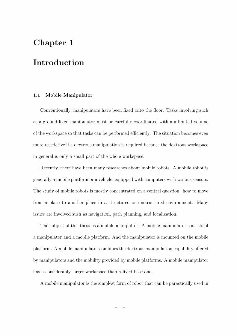
1.1 Mobile Manipulator
Conventionally, manipulators have been fixed onto the floor. Tasks involving such
as a ground-fixed manipulator must be carefully coordinated within a limited volume
of the workspace so that tasks can be performed efficiently. The situation becomes even
more restrictive if a dextrous manipulation is required because the dextrous workspace
in general is only a small part of the whole workspace.
Recently, there have been many researches about mobile robots. A mobile robot is
generally a mobile platform or a vehicle, equipped with computers with various sensors.
The study of mobile robots is mostly concentrated on a central question: how to move
from a place to another place in a structured or unstructured environment. Many
issues are involved sush as navigation, path planning, and localization.
The subject of this thesis is a mobile manipultor. A mobile manipulator consists of
a manipulator and a mobile platform. And the manipulator is mounted on the mobile
platform. A mobile manipulator combines the dextrous manipulation capability offered
by manipulators and the mobility provided by mobile platforms. A mobile manipulator
has a considerably larger workspace than a fixed-base one.
A mobile manipulator is the simplest form of robot that can be paractically used in
– 1 –
various fileds because of its manipulability and mobility that are the most important
features of robots. Many kinds of robots can be considered as a mobile manipulator
in the view of mobility and manipulability. Also there are many potential applications
of mobile manipulators in the fields of manufacturing, nuclear reactor maintenance,
construction, military, and planetary exploration. Therefore mobile manipulators have
many important research problems.
The goal of this thesis is to control nonholonomic constrained mobile manipula-
tors using two-layer neural network. There are a number of challenging problems in
control of mobile manipulators due to the structural complexity. In this thesis, the
nonholonomic constraint to which a wheeled mobile platform is subject, and the non-
linear dynamics with the dynamic interaction between the mobile platform and the
manipulator are mainly considered.
1.2 Related Research
In this section, the related researches are reviewed. The study of control of mobile
manipulators spans several different research areas. Some of them have been extensively
studied while others are fairly new and relatively little research has been devoted.
Major issues realated to the topic of this thesis include the kinematic and dynamic
modeling, the control of wheeled mobile platforms, and the nonlinear dynamics with
the dynamic interaction between the manipulator and the mobile platform.
– 2 –
1.2.1 Control of Nonholonomic constrained Mobile Platforms
Motion control of the mobile platforms is mostly divided into two approaches, i.e.,
open-loop control and closed-loop control. For the closed-loop control approach used
in this study, Kanayama [1] used a two-wheeled steering model for tracking control
and proved the asymptotic convergence of the linearized system to the desired trajec-
tory by using Lyapunov function. Fierro and Lewis [2] represented a control struc-
ture that makes possible the intergation of a kinematic controller and a neural net-
work computed-torque controller for nonholonomic mobile robots. A combined kine-
matic/torque control law is developed using backstepping and stability is guaranteed
by Lyapunov function.
1.2.2 Control of Mobile Manipulators
Li and Frank [3] investigated an inverse kinematics and stability of a three-link
manipulator mounted on a linearly translating vehicle. It is derived that the sufficient
conditions to prevent the vehicle from tipping over. Dubowsky and Tanner [4] studied
the compensation of a dynamic disturbance caused by a vehicle motion to a manipulator
by deriving a set of linearized equations of motion for a 3-DOF planar manipulator atop
a moving base, and verified the result of a dynamic compensation through simulation
and experiment. In the experiment, a vertical linear motion of the base is considered
with a full measurement of the base motion, i.e, position, velocity, and acceleration.
Lie and Lewis [5] described a decentralized robust controller for a mobile manipulator
by considering the platform and the manipulator as two separate systems with which
– 3 –
two interconnected subsystems are stable if the unknown interconnections are bounded.
The model, used for simulation, consists of a two-link manipulator attached on a planar
base in which the angular motion of the base is excluded although it is included in the
equation of motion. Hootsmans [6] derived the Mobile Manipulator Jacobian Transpose
Algorithm with which a manipulator achieves a desired trajectory in the presence of
dynamic disturbance from a softly-suspended platform. It was shown that, even with
a limited sensing capability, the system is able to perform reasonably well with the
proposed algorithm. But only holonomic constrains are taken into account. Among
the previous works on mobile manipulators, the works reported in [3], [4], [5] and [6]
mention or treat the dynamic interaction in an explicit form. The motivation for much
of the previous work stems from identifying the stability criteria so that the vehicle
does not tip over.
Yamamoto [7] investigated modeling, control, and cooridination of mobile manipula-
tors. Coordination algorithm was developed to coordinate manipulatoion and mobility
of a single mobile manipulator. Chung and Velinsky [8] developed an interaction con-
troller that is composed of a robust adaptive controller and an input-output linearizing
controller for mobile manipulator control. Lin and Goldenberg [9] developed a neu-
ral network based methodelogy for the motion control of mobile manipulators subject
to kinematic constraint. The dynamics of the mobile manipulator is assumed to be
completely unknown, and is identified on-line by the neural network estimator. Dong
[10] proposed adaptive controller for the trajectory and force tracking control of mobile
manipulators subject to holonomic and nonholonomic constraints with unknown inter-
– 4 –
tia parameters. Wang [11] presented robust control strategies to control the holonomic
mechanical systems and a class of nonholonomic systems in the presence of uncertain-
ties and disturbances. Li [12] presented adaptive robust force/motion control strategies
for a mobile manipulator under both holonomic and nonholonomic constraints in the
presence of uncertainties and disturbances. The stablity of the closed-loop system and
the boundedness of tracking errors are proved using Lyapunov stability synthesis. Gao
[13] presented an intelligent controller based on RBF neural network for the coordi-
nating control of the mobile manipulator. Calculating the extensive Jacobian matrix
is rather difficult, RBF neural network is adapted to approach the kinematic model of
the system and achieve the decoupling results. White [14] adapted that the indepen-
dent controller for mobile manipulators, developed within each decoupled space that
is external(task) space and internal(null) space, facilitates active internal reconfigura-
tion and resolves redundancy at the dynamic level. These algorithms are evaluated
within an implementation framework that emphasizes both virtual prototyping and
hardware-in-the-loop testing with representative case studies. Hirata [15] proposed
motion control algorithm of multiple mobile manipulators for handling a single object
in cooperation with a human, and the coordinated motion control algorithm between
the manipulator and the mobile base for each mobile manipulator.
1.3 Motivation and Contribution of this Work
There are a number of challenging problems in control of mobile manipulators due
to the structural complexity - for example, the redundancy created by combing the
– 5 –
manipulator and the mobile platform, the nonholonomic constraints to which wheeled
mobile platforms are subjected, and the dynamic interaction between the mobile plat-
form and the manipulator. In this thesis, the nonholonomic constraint of the mobile
platform and the nonlinear and coupled dynamics are mainly considered.
There are many researches to control nonholonomic constrained mobile platforms.
In this study, the closed-loop kinematic controller suggested by Kanayama [1] is used.
In this method, the reference velocity input to the steering system of a mobile platform
is calculated from the tracking errors like position and orientation. In this approach,
if the mobile platform can track a class of velocity control inputs, then tracking, path
following and stablitization about a desired posture may be solved [2]. So the next
work is to design controller that guarantees perfect velocity tracking.
To control mobile manipulators with the nonlinear and coupled dynamics, the mo-
bile manipultor dynamic model is required but obtaining preciese dynamic model is
not easy. In computed torque method, the performances are influenced by the dy-
namic model error. When a mobile manipulator operates at a relatively high speed,
ignoring the mobile manipulator dynamics and the dynamic interaction between the
manipulator and the mobile platform, it may cause unbearable vibrations of the system
[6]. Therefore the neural network has been adapted to control the systems that have
complex nonlinear dynamics and dynamic interaction, because of its strong learning
capability. In the neural network based control, the neural network estimates unknown
nonlinear dynamic models and uses it for compensation. Therefore the neural network
based approach can deal with the control of nonlinear systems that may not be linearly
– 6 –
parameterizable, as required in the adaptive approach.
The goal of this thesis is to control nonholonomic constrained mobile manipulators
using two-layer neural network. The position and orientation of the mobile platform
and the joints of the manipulator are controlled, and the control laws based on two-
layer neural network is derived. The tracking stability of the closed-loop system, the
convergence of the neural network weight-updating process and boundedness of the
neural network weight estimation errors are all guaranteed using Lyapunov function.
In [9], the neural network based control for mobile manipulators was already sug-
gested. It is based on the neural network f(x) = W Tφ(x) with one-layer weights that
are updated. This neural network controller displayed good performance, even though
it required no detailed knowledge of the system. However, using this one-layer neural
network requires to select the activation functions φ(x) corresponding to a basis set
for smooth function f(x). If the activation functions are not properly selected, then
there will be more approximation errors. There is not systematic way to select acti-
vation functions. In this research, a controller based on the two-layer neural network
f(x) = W Tφ(V Tx) is derived. This neural network requires no preselection of the
basis set. In effect, by the weight updating algorithm for first-layer, the neural network
can learn its own basis set for the system nonlinearities. Thus, the main contribution
of this thesis is to improve the performance of the neural network of [9] by enhanc-
ing the weight updating mechanism. Moreover, by the weight updating algorithm for
first-layer, the activation functions corresponding to the basis set is selected automat-
ically. Therefore more precise estimation of a function can be expected. The stability
– 7 –
including the weight updating algorithm is guaranteed through Lyapunov function.
1.4 Organization of the Thesis
This thesis is organized as follows. The dynamics of mobile manipulators is repre-
sented in Chapter 2. Section 2.2 describes the concepts of nonholonomic constraint.
In Section 2.3, the constraint equations are represented with some analysis. In Section
2.4, The dynamic equations of mobile manipulators are represented.
In Chapter 3, the control structure of mobile manipulators is represented. In Section
3.2, nonholonomic constrained mobile platform control is represented by considering
the steering system. In Section 3.3, the Lypunov functions for mobile manipulators
are given. In Section 3.4, the neural network for function approximation is suggested
with some properties. In section 3.5, the control structure for mobile manipulators
is suggested with the neural network control and the neural network weight updating
algorithm.
In Chapter 4, the suggested control laws based on neural network with the control
structure is implemented on simulation. In Chapter 5, the experments of the suggested
control laws performed using 2-axis planar manipulator. Through the simulation and
the experiments, the validity of the suggested control is verified.
Finally, Conclusion with some discussions are given in Chapter 6.
– 8 –
Chapter 2
Modeling of Mobile Manipulators
2.1 Introduction
In this chapter, the dynamic model of nonholonomic constrained mobile manipula-
tors is represented. The definition of nonholonomic constraint is described. Moreover
the constraint equations of the wheeled mobile platform that is used in this study is
given with some analysis. Finally, it is derived that the dynamic equations of the
nonholonomic constrained mobile manipulator with some properties. In the dynamic
equations, it it representd that the nonholonomic constraint and the nonlinar dynamics
with dynamic interation between the mobile platform and the manipulator.
2.2 Nonholonomic Constraint
A classical Example of nonholonomic systems is a rigid disk rolling on a horizontal
plant without slippage [18], which is equivalent, from the control perspective, to a
wheeled cart driven by two wheel. As a matter of fact, a car-like system in general is
a nonholonomic system except a few examples of omnidirectional vehicles.
Constraints can be written in the form of
wi(q)q = 0, i = 1, ..., k, (2.1)
where wi ∈ R1×n are row vectors. It is assumed that wi are linearly independent at
– 9 –
each point q ∈ Rn, becuase the dependent constraints can be eliminated. Each wi
describes one constraint on the direcions in which q is permitted to take values.
A constraint is said holonomic if it restricts the motion of a system to a smooth
hypersurface of the configuration space. In terms of differential geometry, this smooth
hyperspace can be called a manifold which is a topological space that is locally difffeo-
morphic1 to Euclidean space Rm. Locally, a holonomic constraint can be represented
as a set of algebraic constraints on the configuration space,
hi(q) = 0, i = 1, ..., k. (2.2)
The dimension of the manifold on which the motioin of the systme evolves is n− k.
A set of k Pfaffinan constraints of the form on equation (2.1) is intergrable if there
exist function hi : Rn → R, i = 1, ..., k such that
hi(q(t)) = 0 ⇐⇒ wq(q)q = 0, i = 1, ..., k. (2.3)
Hence, a set of Pfaffian constraints is intergrable if it is equivalent to a set of holo-
nomic constrains. An intergrable Pfaffian constraint is called a holonomic constraint,
althought strictly spaeaking the former is described by a set of velocity constraints and
the latter by a set of functions. A set of Pfaffian constrains is said to nonholonomic if
it it not equivalent to a set of holonomic constraints [18].
– 10 –
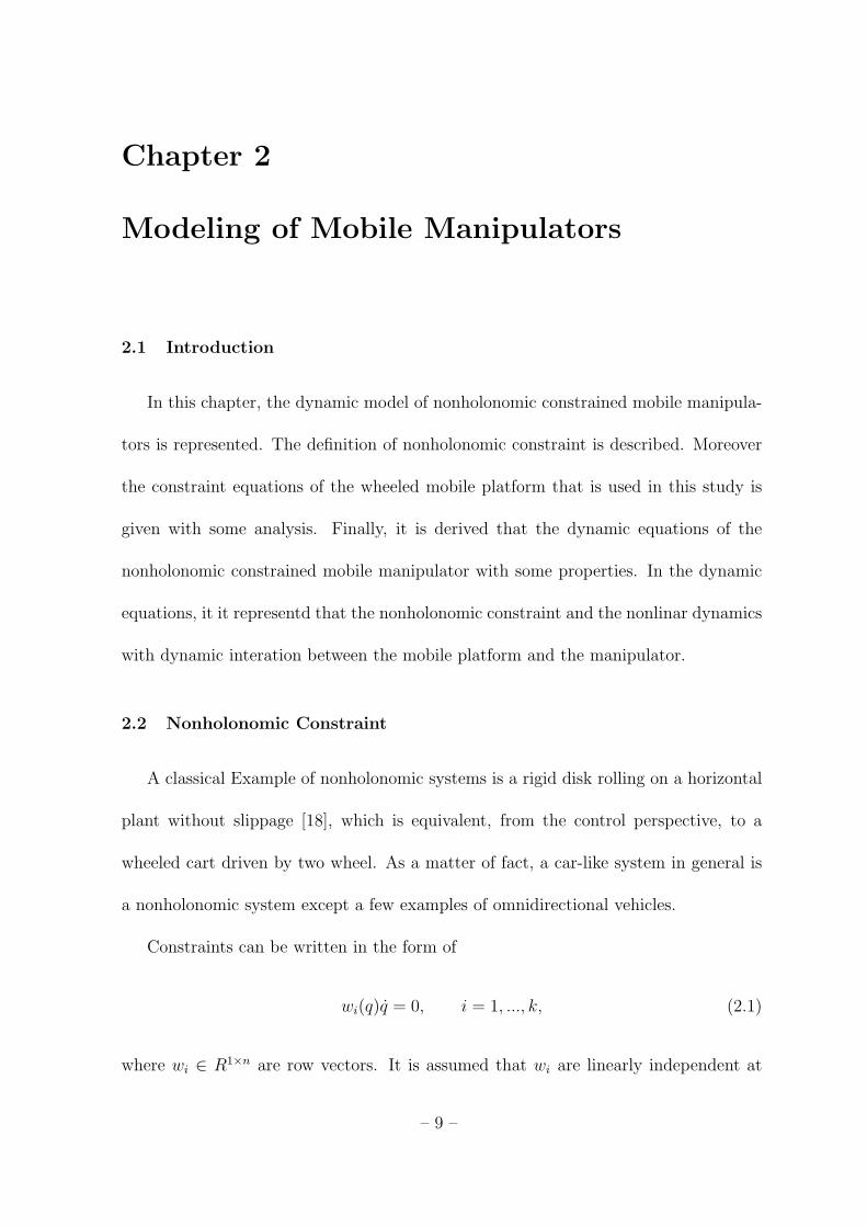
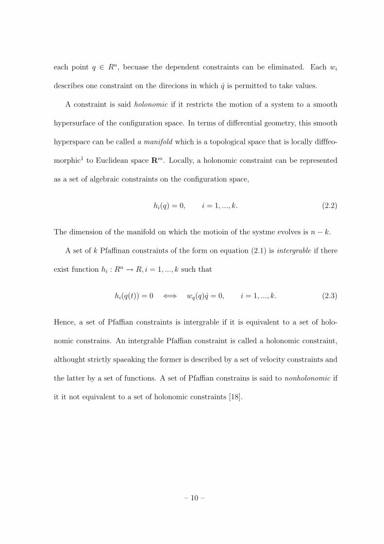
Figure 2.1: Schematic of a wheeled mobile platform.
2.3 Constraint Equations
The schematic of a wheeled mobile platform is shown in figure 2.1. The mobile
platform has two coaxial wheels which are driven independently. The mobile platform
is subject to constraint.
The nonholonomic constraint of the mobile platform states that the mobile platform
can only move in the direction normal to the axis of the driving wheels, i.e., the mobile
platform satisfies the conditions of pure rolling and nonslipping.
yo cosφ− xo sinφ = 0 (2.4)
where (xo, yo) is coordinates of point Po in the inertia frame Σw, and φ is the heading
angle of the mobile platform measured from wX-axis.
1A diffeomorphism is simply a differentiable function whose inverse exists and is also differentiable
[19].
– 11 –
Let the Lagrange coordinates of the mobile platform be q = [xo, yo, φ]T . The con-
straint can be written as follows
A(q)q = 0 (2.5)
where
A(a) = [− sinφ cosφ 0]. (2.6)
A 3× 2 dimensional matrix is defined as follows.
S(q) = [s1(q) s2(q)] =
cosφ 0
sinφ 0
0 1
(2.7)
The two independent columns of matrix S(q) are in the null space of matrix A(q), that
is, A(q)S(q) = 0. It is defined that the distribution is a span of the columns of S(q).
∆ = span{s1(q), s2(q)} (2.8)
The involutivity of the distribution ∆ determines the number of holonomic or nonholo-
nomic constraints. If ∆ is involutive, from the Frobenius theorem, all the constraints
are intergrable (thus holonomic) [18]. If the smallest involutive distribution containing
∆ (denoted by ∆∗) spans the entire 3-dimentional space, all the constraints are non-
holonomic. If dim(∆∗) = 3 − k, then k constrains are holonimic and the others are
nonholonomic.
To verify the involutivity of ∆, the Lie bracket of s1(q) and s2(q) is computed.
s3(q) = [ s1(q), s2(q) ] =∂s2
∂qs1 −
∂s1
∂qs2 =
− sinφ
cosφ
0
(2.9)
– 12 –
is lineary independent of s1(q) and s2(q). The distribution spanned by s1(q), s2(q),
and s3(q) is involutive. Therefore, the involutive closure of the distribution is
∆∗ = span{s1(q), s2(q), s3(q)}. (2.10)
Therefore the constraint (2.4) is nonholonomic constraint.
2.4 Dynamic Modeling of Mobile Manipulators
The mobile manipulator dynamics is written as [9]
M(q)q + C(q, q)q + F (q, q) + AT (q)λ+ τd = E(q)τ
Mv Mvr
Mrv Mr
qv
qr
+
Cv Cvr
Crv Cr
qv
qr
+
F1
F2
+
ATv (qv)λ
0
+
τd1
τd2
=
Evτv
τr
(2.11)
where the kinematic constraint is described by
Av(qv)qv = 0. (2.12)
qv ∈ Rm denotes the generalized coordinates appearing in the constraint equation
(2.12), and qr ∈ Rn is the free generalized coordinates; p = m + n. M(q) ∈ Rp×p is
the inertia matrix, C(q, q) ∈ Rp×p is the coriolis/centripetal matrix, Av(qv) ∈ Rr×m
is constraint matrix, λ ∈ Rr denotes the vector of Lagrange multipliers corresponding
to the kinematic constraint, τv ∈ Rm−r is the input torque to the mobile platform,
Ev ∈ Rm×(m−r) is the input transformation matrix, τr ∈ Rn is the input torque for
– 13 –
the manipulator, F (q, q) ∈ Rp is friction and gravity vector, and τd1 and τd2 are
disturbances bounded by ‖τd1‖ ≤ τ1N and ‖τd2‖ ≤ τ2N with τ1N and τ2N some positive
constants. The first row of (2.11) with the constraint equation (2.12) represents the
mobile platform dynamics, and the second row of (2.11) represents the manipulator
dynamics.
In (2.11), the following properties hold [9] [16].
Property 1 (Parameter Boundedness)
MminIn ≤ M(q) ≤MmaxIn
C(q, q) ≤ Cb(q)‖q‖ (2.13)
where Mmin, Mmax is positive scalar constants which are dependent on the mass proper-
ties and constraint matrix; In is p×p identity matrix; Cb(q) is positive definite function
of q.
Property 2 (Skew Symmetricity)
M − 2C = −(M − 2C)T
M = C + CT . (2.14)
Property 3 Mv and Mr are both symmetric and positive definite, and
Mv − 2Cv = −(Mv − 2Cv)T
Mr − 2Cr = −(Mr − 2Cr)T . (2.15)
– 14 –
Property 4
Mrv = Crv + CTvr
Mvr = MTrv. (2.16)
Sv(qv) ∈ Rm×(m−r) represents a full rank matrix that spans the null space of Av(qv)
defined in (2.12), i.e.,
ST (qv)ATv (qv) = 0. (2.17)
From (2.17), an auxiliary vector v(t) ∈ Rm−r exists such that for all t
qv = S(qv)v(t) (2.18)
and
qv = S(qv)v + S(qv)v. (2.19)
Equation (2.18) is called the steering system and v(t) can be regarded as a velocity
input vector steering the state vector q in the state space.
From the first m-equations of (2.11),
Mv qv +Mvrqr + Cv qv + Cvrqr + F1 + ATv (qv)λ+ τd1 = Evτv. (2.20)
(2.17) is used to eliminate the constraint force λ. Multiplying ST to the both sides of
(2.20), the following is obtained
STMv qv + STMvrqr + STCv qv + STCvrqr + STF1 + ST τd1 = STEvτv. (2.21)
Substituting (2.18) and (2.19)
STMvSv+STMvSv+STMvrqr+STCvSv+STCvrqr+STF1 +ST τd1 = STEvτv. (2.22)
– 15 –
Rewrite (2.22) in a compact form as
Mvv + Cvv + f1 + τd1 = τv (2.23)
where Mv = STMvS, Cv = STCvS + STMvS, τd1 = ST τd1; ||τd1|| ≤ τ1N with τ1N
positive constant (notice that both τd1 and S are bounded), and
τv = STEvτv (2.24)
f1 = ST (Mvrqr + Cvrqr + F1) (2.25)
where f1 consists of the gravitational and frictional force vector F1 and the dynamic
interaction with the manipulator (i.e., Mvrqr + Cvrqr).
Property 5 ˙M v − 2Cv is skew-symmetric [9].
Consider the second n-equations of (2.11)
Mrv qv +Mrqr + Crv qv + Crqr + F2 + τd2 = τr. (2.26)
Rearrange (2.26) as follows:
Mrqr + Crqr + (Mrv qv + Crv qv + F2 + τd2) = τr. (2.27)
Equation (2.27) represents the dynamic equation of the manipulator. The terms in
brackets consists of the dynamic interaction term (i.e., Mrv qv+Crv qv), the gravitational
and friction force vector F2, and the disturbance on the manipulator.
Equations (2.18), (2.23) and (2.27) form the dynamic model of the mobile manip-
ulators subjected to the kinematic constraints.
– 16 –
Chapter 3
Mobile Manipulator Control
3.1 Introduction
In this chapter, the control structure of mobile manipulators is represented by
considering nonholonomic constraint and nonlinear and coupled dynamics. In this
control structure, the kinematic controller is used to treat nonholonomic constraint.
Moreover the neural network with the weight updating algorithm is suggested to treat
nonlinear and coupled dynamics. The control laws τv and τr based on the neural
network with the weight updating algorithm are derived. The tracking stability of the
closed-loop system, the convergence of the neural network weight-updating process and
boundedness of the neural network weight estimation errors are all guaranteed using
Lyapunov function.
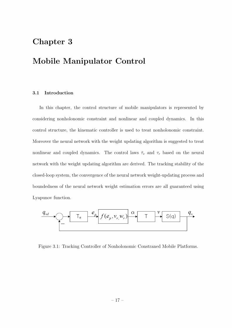
Figure 3.1: Tracking Controller of Nonholonomic Constraned Mobile Platforms.
– 17 –
3.2 Nonholonomic Constrained Mobile Platform Control
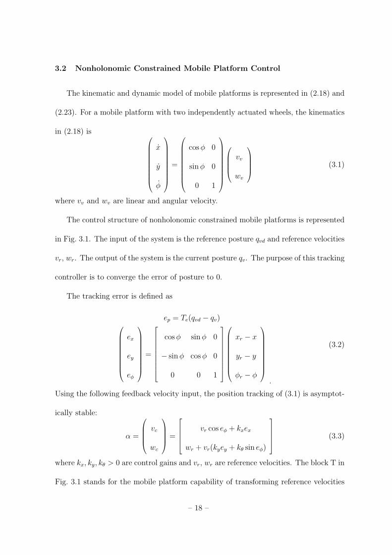
The kinematic and dynamic model of mobile platforms is represented in (2.18) and
(2.23). For a mobile platform with two independently actuated wheels, the kinematics
in (2.18) is
x
y
φ
=
cosφ 0
sinφ 0
0 1
vv
wv
(3.1)
where vv and wv are linear and angular velocity.
The control structure of nonholonomic constrained mobile platforms is represented
in Fig. 3.1. The input of the system is the reference posture qvd and reference velocities
vr, wr. The output of the system is the current posture qv. The purpose of this tracking
controller is to converge the error of posture to 0.
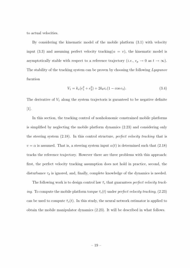
The tracking error is defined as
ep = Te(qvd − qv)
ex
ey
eφ
=
cosφ sinφ 0
− sinφ cosφ 0
0 0 1
xr − x
yr − y
φr − φ
.
(3.2)
Using the following feedback velocity input, the position tracking of (3.1) is asymptot-
ically stable:
α =
vc
wc
=
vr cos eφ + kxex
wr + vr(kyey + kθ sin eφ)
(3.3)
where kx, ky, kθ > 0 are control gains and vr, wr are reference velocities. The block T in
Fig. 3.1 stands for the mobile platform capability of transforming reference velocities
– 18 –
to actual velocities.
By considering the kinematic model of the mobile platform (3.1) with velocity
input (3.3) and assuming perfect velocity tracking(α = v), the kinematic model is
asymptotically stable with respect to a reference trajectory (i.e., ep → 0 as t → ∞).
The stability of the tracking system can be proven by choosing the following Lyapunov
fucntion
V1 = kx(e21 + e22) + 2kθvr(1− cos e3). (3.4)
The derivative of V1 along the system trajectoris is guranteed to be negative definite
[1].
In this section, the tracking control of nonholonomic constrained mobile platforms
is simplified by neglecting the mobile platform dynamics (2.23) and considering only
the steering system (2.18). In this control structure, perfect velocity tracking that is
v = α is assumed. That is, a steering system input α(t) is determined such that (2.18)
tracks the reference trajectory. However there are three problems with this approach:
first, the perfect velocity tracking assumption does not hold in practice, second, the
disturbance τd is ignored, and, finally, complete knowledge of the dynamics is needed.
The following work is to design control law τv that guarantees perfect velocity track-
ing. To compute the mobile platform torque τv(t) under perfect velocity tracking, (2.23)
can be used to compute τv(t). In this study, the neural network estimator is applied to
obtain the mobile manipulator dynamics (2.23). It will be described in what follows.
– 19 –
3.3 Lypunov functions for the mobile manipulator
In this section, the Lyapunov functions for the mobile manipulator are derived [9].
The desired trjectory satisfies the following assumption 3.3.1.
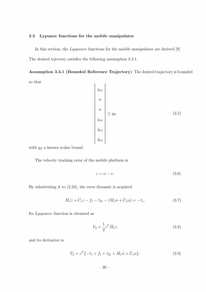
Assumption 3.3.1 (Bounded Reference Trajectory) The desired trajectory is bounded
so that ∥∥∥∥∥∥∥∥∥∥∥∥∥∥∥∥∥∥∥∥∥∥∥∥∥∥∥∥∥
qvd
α
α
qrd
qrd
qrd
∥∥∥∥∥∥∥∥∥∥∥∥∥∥∥∥∥∥∥∥∥∥∥∥∥∥∥∥∥
≤ qB (3.5)
with qB a known scalar bound.
The velocity tracking error of the mobile platform is
z = α− v. (3.6)
By substituting it to (2.23), the error dynamic is acquired
Mvz + Cvz − f1 − τd1 − (Mvα + Cvα) = −τv. (3.7)
Its Lyapunov function is obtained as
V2 =1
2zTMvz (3.8)
and its derivative is
V2 = zT{−τv + f1 + τd1 + Mvα + Cvα}. (3.9)
– 20 –
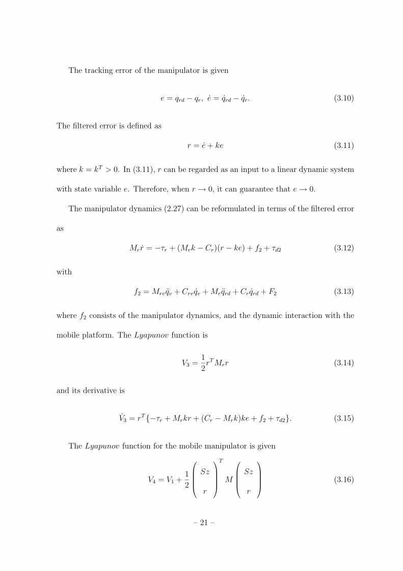
The tracking error of the manipulator is given
e = qrd − qr, e = qrd − qr. (3.10)
The filtered error is defined as
r = e+ ke (3.11)
where k = kT > 0. In (3.11), r can be regarded as an input to a linear dynamic system
with state variable e. Therefore, when r → 0, it can guarantee that e→ 0.
The manipulator dynamics (2.27) can be reformulated in terms of the filtered error
as
Mrr = −τr + (Mrk − Cr)(r − ke) + f2 + τd2 (3.12)
with
f2 = Mrv qv + Crv qv +Mrqrd + Crqrd + F2 (3.13)
where f2 consists of the manipulator dynamics, and the dynamic interaction with the
mobile platform. The Lyapunov function is
V3 =1
2rTMrr (3.14)
and its derivative is
V3 = rT{−τr +Mrkr + (Cr −Mrk)ke+ f2 + τd2}. (3.15)
The Lyapunov function for the mobile manipulator is given
V4 = V1 +1
2
Sz
r
T
M
Sz
r
(3.16)
– 21 –
and can be derived to
V4 = V1 + V2 + V3 + rTMTvr(Sz). (3.17)
Its derivative is
V4 = V1 + V2 + V3 +d
dt{rTMrv(Sz)}. (3.18)
By deriving this, the following is obtained
V4 ≤ zT{−τv + Ψ1}+ rT{−τr + Ψ2}+ zT τd1 + rT τd2 (3.19)
with the unknown nonlinear terms
Ψ1 = Mvα + Cvα + f1 + ST{Cvrke+Mvrk(r − ke)} (3.20)
Ψ2 = Mrkr + (Cr −Mrk)ke+ f2 +MrvSα +MrvSα + CrvSα (3.21)
where
f1 = ST{Mvrqrd + Cvrqrd + F1}
f2 = Mrqrd + Crqrd + F2.
(3.22)
The nonlinear term Ψ1 and Ψ2 in (3.20) and (3.21) are the unknown mobile manipulator
function and provide the amount of torque necessary to drive the system along its path.
In this thesis, it is to be identified on-line by neural network and used to compensation
the nonlinear and coupled dynamics of mobile manipulators. More specifically they
represent coupled inertia terms, coupled coriolis/centripetal terms, the gravitational
and frictional force vector terms taking place due to the coupling between the mobile
platform and manipulator.
– 22 –
3.4 Neural Network Approximation
According to the universal approximation ability of the NN(Neural Network), Ψ1
and Ψ2 defined in (3.20) and (3.21), respectively, may be identified using NN with
sufficiently high number of hidden-layer neurons such that
Ψ1 = W T1 σ(V T
1 x) + ε1(x)
Ψ2 = W T2 σ(V T
2 x) + ε2(x)
(3.23)
where x is the input pattern to the NN defined as
x ≡[qTvd αT αT qTv zT eT rT qTrd qTrd qTrd
]T∈ R(5m+5n−3r)
. (3.24)
Define the matrix of all the NN weights as
Z =
W 0
0 V
.
(3.25)
Z1 ∈ R(n1+5m+5n−3r)×(m−r+n1) and Z2 ∈ R(n2+5m+5n−3r)×(n+n2) are ideal and unknown
weights, respectively, which are assumed to be constant and bounded
‖Z1‖F ≤ Z1B, ‖Z2‖F ≤ Z2B (3.26)
with Z1B and Z2B some known positive constants and ‖ · ‖F the Frobenius norm1;
n1 and n2 are the numbers of hidden-layer neurons of the two NN, respectively; the
approximation error ε1 ∈ Rm−r, ε2 ∈ Rn are bounded by ||ε1|| ≤ ε1N and ||ε2|| ≤ ε2N
with ε1N and ε2N two positive constants; σ1(s) ∈ Rn1 and σ2(s) ∈ Rn2 are properly
chosen basis functions for the hidden-layer neurons of the two nets where s = V Tx,
1The Frobenius norm of a matrix is defined as the root of the sum of squares fo all elements
‖A‖2F = tr(AT A).
– 23 –
with x as the input pattern of the input layers to the two nets. The basis functions
can be chosen as the Sigmoid function defined as
σ(s) =1
1 + e−s .(3.27)
The estimations of Ψ1 and Ψ2 are given by
Ψ1 = W T1 σ(V T
1 x)
Ψ2 = W T2 σ(V T
2 x)
(3.28)
with V1, W1, V2 and W2 the actual values of the NN weights given by the NN weight
updating algorithm to be specified. Note that V1, W1, V2 and W2 are estimation of the
ideal weight values and define the weight deviaitions or weight estimation errors as
V = V − V , W = W − W , Z = Z − Z. (3.29)
Define the hidden-layer output error for a given x as
σ = σ − σ ≡ σ(V Tx)− σ(V Tx). (3.30)
The Taylor series expansion of σ(x) for a given x may be written as
σ(V Tx) ≡ σ(V Tx) + σ′(V Tx)V Tx+O(V Tx)2, (3.31)
with the Jacobian matrix
σ′(z) ≡ dσ(z)
dz
∣∣∣∣z=z
(3.32)
and O(z)2 denoting terms of order two. Denoting σ′ = σ′(V Tx), the following is derived
σ = σ′(V Tx)V Tx+O(V Tx)2 = σ′V Tx+O(V Tx)2. (3.33)
– 24 –
The importance of equation (3.33) is that it replaces σ, which is nonlinear in V , by
an expression linear in V plus higer-order terms. This will allow to determine the NN
weight updating algorithm for V in subsequent derivations.
Different bounds may be put on the Taylor series higher-order terms depending on
the choice for activation fucntions σ(·). Noting that
O(V Tx)2 = [σ(V Tx)− σ(V Tx)]− σ′V Tx (3.34)
one has the following. The numbering of the constants ci take up after the c0, c1, c2,
c8, c9 and c10 defined in Lemma 3.4.1.
Lemma 3.4.1 (Bound on NN input x) For each t, x(t) is bounded by
‖x‖ ≤ c1 + c2‖z‖ ≤ qB + c0‖z(0)‖+ c2‖z‖ (3.35)
and
‖x‖ ≤ c9 + c10‖r‖ ≤ qB + c8‖r(0)‖+ c10‖r‖ (3.36)
for computable positive constant c0, c1, c2, c8, c9, c10 [16].
Lemma 3.4.2 (Bounds on Taylor Series Higher-Order Terms) For sigmoid ac-
tivation function, the higher-order terms in the Taylor series are bounded by
‖O(V T1 x)‖ ≤ c3 + c4qB‖V1‖F + c5‖V1‖F‖z‖ (3.37)
and
‖O(V T2 x)‖ ≤ c11 + c12qB‖V2‖F + c13‖V2‖F‖r‖ (3.38)
where ci are computable positive constants [16].
– 25 –
K2
Robustterm
k
d/dt
Robustterm
K1
NeuralNetwork
S(q)KinematicController
Te
1ˆ
v
rdqr
2ˆ
1( )v t
2 ( )v t
e r
pe zv vq
rq
vdqvq
MobileManipulator
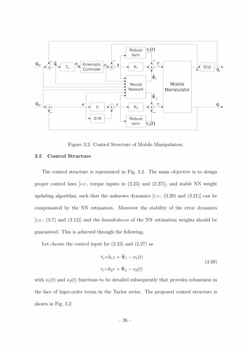
Figure 3.2: Control Structure of Mobile Manipulators.
3.5 Control Structure
The control structure is represented in Fig. 3.2. The main objective is to design
proper control laws [i.e., torque inputs in (2.23) and (2.27)], and stable NN weight
updating algorithm, such that the unknown dynamics [i.e., (3.20) and (3.21)] can be
compensated by the NN estimators. Moreover the stability of the error dynamics
[i.e., (3.7) and (3.12)] and the boundedness of the NN estimation weights should be
guaranteed. This is achieved through the following.
Let choose the control input for (2.23) and (2.27) as
τv=k1z + Ψ1 − ν1(t)
τr=k2r + Ψ2 − ν2(t)
(3.39)
with ν1(t) and ν2(t) functions to be detailed subsequently that provides robustness in
the face of higer-order terms in the Taylor series. The proposed control structure is
shown in Fig. 3.2.
– 26 –
Substituting (3.39) into (3.19) yields
V4 ≤ zT{−k1z − Ψ1 + ν1 + Ψ1}+ rT τd2 + rT{−k2r − Ψ2 + ν2 + Ψ2}+ zT τd1 (3.40)
≤ −k1zT z + zTν1 + zT{Ψ1 − Ψ1}+ zT τd1 − k2r
T r + rTν2 + rT{Ψ2 − Ψ2}+ rT τd2.
Using (3.23), (3.28) and (3.33),
Ψ1 − Ψ1 = W T1 (σ1 − σ
′1V
T1 x) + W T
1 σ′1V
T1 x+ W T
1 σ′1V
T1 x+W T
1 O(V T1 x)2 + ε1
Ψ2 − Ψ2 = W T2 (σ2 − σ
′2V
T2 x) + W T
2 σ′2V
T2 x+ W T
2 σ′2V
T2 x+W T
2 O(V T2 x)2 + ε2.
(3.41)
The inequality is obtained by substitute (3.41) into (3.40),
V4 ≤ − k1zT z + zTν1 + zTw1 + zT{W T
1 (σ1 − σ′
1VT1 x) + W T
1 σ′
1VT1 x}
− k2rT r + rTν2 + rTw2 + rT{W T
2 (σ2 − σ′
2VT2 x) + W T
2 σ′
2VT2 x} (3.42)
where
w1(t) = W T1 σ
′1V
T1 x+W T
1 O(V T1 x)2 + ε1 + τd1
w2(t) = W T2 σ
′2V
T2 x+W T
2 O(V T2 x)2 + ε2 + τd2
.
(3.43)
Lemma 3.5.1 (Bounds on the Disturbance Term) The disturbance term (3.43)
is bounded according to
‖w1(t)‖ ≤ (ε1N + d1B + c3Z1B) + c6Z1B‖Z1‖F + c7Z1B‖Z1‖F‖z‖ (3.44)
‖w1(t)‖ ≤ C0 + C1‖Z1‖F + C2‖Z1‖F‖z‖ (3.45)
and
‖w2(t)‖ ≤ (ε2N + d2B + c11Z2B) + c14Z2B‖Z2‖F + c15Z2B‖Z2‖F‖r‖ (3.46)
‖w2(t)‖ ≤ C3 + C4‖Z2‖F + C5‖Z2‖F‖r‖ (3.47)
with Ci known positive constants [16].
– 27 –
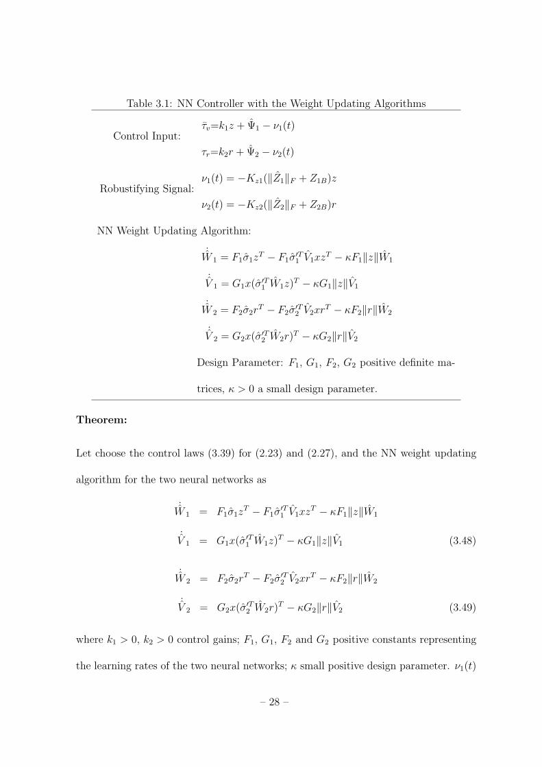
Table 3.1: NN Controller with the Weight Updating Algorithms
Control Input:τv=k1z + Ψ1 − ν1(t)
τr=k2r + Ψ2 − ν2(t)
Robustifying Signal:ν1(t) = −Kz1(‖Z1‖F + Z1B)z
ν2(t) = −Kz2(‖Z2‖F + Z2B)r
NN Weight Updating Algorithm:
˙W 1 = F1σ1z
T − F1σ′T1 V1xz
T − κF1‖z‖W1
˙V 1 = G1x(σ′T1 W1z)T − κG1‖z‖V1
˙W 2 = F2σ2r
T − F2σ′T2 V2xr
T − κF2‖r‖W2
˙V 2 = G2x(σ′T2 W2r)
T − κG2‖r‖V2
Design Parameter: F1, G1, F2, G2 positive definite ma-
trices, κ > 0 a small design parameter.
Theorem:
Let choose the control laws (3.39) for (2.23) and (2.27), and the NN weight updating
algorithm for the two neural networks as
˙W 1 = F1σ1z
T − F1σ′T1 V1xz
T − κF1‖z‖W1
˙V 1 = G1x(σ′T1 W1z)T − κG1‖z‖V1 (3.48)
˙W 2 = F2σ2r
T − F2σ′T2 V2xr
T − κF2‖r‖W2
˙V 2 = G2x(σ′T2 W2r)
T − κG2‖r‖V2 (3.49)
where k1 > 0, k2 > 0 control gains; F1, G1, F2 and G2 positive constants representing
the learning rates of the two neural networks; κ small positive design parameter. ν1(t)
– 28 –
and ν2(t) are auxiliary signals to provide robustness in the face of disturbances and
modelling errors and given as
ν1(t) = −Kz1(‖Z1‖F + Z1B)z
ν2(t) = −Kz2(‖Z2‖F + Z2B)r (3.50)
with gain
Kz1 > C2 (3.51)
Kz2 > C5 (3.52)
where C2 and C5 is represented in Lemma 3.5.1.
By properly choosing the control gains and design parameters, then the tracking
errors of error dynamics described by (2.18), (3.7) and (3.12), and the NN estimation
weights V1, W1, V2 and W2 are all guaranteed to be uniformly ultimately bounded.
The proposed mobile manipulator controller (3.39) comprises two independent con-
trollers for the mobile platform and the manipulator. The unknown dynamics Ψ1 and
Ψ2, which model the coupled dynamics between the mobile platform and the manipu-
lator, are, respectively, identified and compensated in real time by the two NN on-line
estimators using the NN learning rules (3.48) and (3.49). In the NN estimators, the
dynamic couplings between the mobile platform and the manipulator are identified by
using the common NN input pattern x [defined in (3.24)] and tracking error-vector z
and r.
– 29 –
Proof of the Theorem:
Let the NN approximation property (3.23) holds for the function Ψ1, Ψ2 given in
(3.20), (3.21) with a given accuracy ε1N and ε2N for all x in the compact set Sx ≡
{x|‖x‖ < bx} with bx > qB. Define Sz ≡ {z|‖z‖ < (bx − qB)/(c0 + c2)} and Sr ≡
{r|‖r‖ < (bx − qB)/(c8 + c10)}. Let z(0) ∈ Sz and r(0) ∈ Sr. Then the approximation
property holds.
The Lyapunov function is chosen as
V = V4 +1
2tr{W T
1 F−11 W1}+
1
2tr{V T
1 G−11 V1}+
1
2tr{W T
2 F−12 W2}+
1
2tr{V T
2 G−12 V2}.
(3.53)
The Lyapunov function V consists of the Lyapunov function V4[proposed in (3.16)] for
a mobile manipulator, and two additional terms which are used to count for the NN
weight updating algorithm. Differentiating (3.53) and substituting (3.19) into it yields
V ≤ −k1zT z + zTw1 + zTν1 − k2r
T r + rTw2 + rTν2 (3.54)
+tr{W1T
(F−11
˙W1 + σ1zT − σ′
1V1xzT )}+ tr{V1
T(G−1
1˙V1 + xzT W1σ
′
1)}
+tr{W2T
(F−12
˙W2 + σ2rT − σ′
2V2xrT )}+ tr{V2
T(G−1
2˙V2 + xrT W2σ
′
2)}.
The NN learning rules give
V ≤ − k1zT z + zT (w1 + ν1)− k2r
T r + rT (w2 + ν2)
+ k ‖z‖ tr{W T1 (W1 − W1)}+ k ‖z‖ tr{V T
1 (V1 − V1)}
+ k ‖r‖ tr{W T2 (W2 − W2)}+ k ‖r‖ tr{V T
2 (V1 − V1)}
≤ − k1zT z + zT (w1 + v1)− k2r
T r + rT (w2 + v2) (3.55)
+ k ‖z‖ tr{ZT1 (Z1 − Z1)}+ k ‖r‖ tr{ZT
2 (Z2 − Z2)}.
– 30 –
Since
tr{ZT (Z − Z)} ≤ Z,−‖Z‖2F< Z
≤ ‖Z‖F‖Z‖F − ‖Z‖2F(3.56)
in [16], there results
V ≤ − k1zT z + ‖z‖ · ‖w1‖+ k ‖z‖ · ‖Z1‖F (Z1B − ‖Z1‖F )−Kz1(‖Z1‖F − Z1B) ‖z‖2
− k2rT r + ‖r‖ · ‖w2‖+ k ‖r‖ · ‖Z2‖F (Z2B − ‖Z2‖F )−Kz2(‖Z2‖F − Z2B) ‖r‖2
≤ − k1 ‖z‖2 + ‖z‖[C0 + C1||Z1||F + C2||z|| · ||Z1||F
]+ k ‖z‖ · ‖Z1‖F (Z1B − ‖Z1‖F )
− k2 ‖r‖2 + ‖r‖[C3 + C4||Z2||F + C5||r|| · ||Z2||F
]+ k ‖r‖ · ‖Z2‖F (Z2B − ‖Z2‖F )
− Kz1(‖Z1‖F − Z1B)‖z‖2 −Kz2(‖Z2‖F − Z2B)‖r‖2 (3.57)
≤ − ‖z‖{k1‖z‖ − k‖Z1‖F (Z1B − ‖Z1‖F )− C0 − C1||Z1||F}
− ‖r‖{k2‖r‖ − k‖Z2‖F (Z2B − ‖Z2‖F )− C3 − C4||Z2||F}.
where Lemma 3.5.1 was used, and the last inequality holds due to (3.51), (3.52).
V is negative as long as the term in braces is positive. Defining C6 = Z1B + C1/k,
C7 = Z2B + C4/k and completing the square yields
k1||z|| − k||Z1||F (Z1B − ||Z1||F )− C0 − C1||Z1||F
= k(||Z1||F − C6/2)2 − kC26/4 + k1||z|| − C0
(3.58)
which is guaranteed positive as long as either
||z|| > C0 + kC26/4
k1
≡ bz (3.59)
or
||Z1||F >C6
2+
√C0
k+C2
6
4≡ bZ1. (3.60)
– 31 –
And
k2||r|| − k||Z2||F (Z2B − ||Z2||F )− C3 − C4||Z2||F}
= k(||Z2||F − C7/2)2 − kC27/4 + k2||r|| − C3
(3.61)
which is guaranteed positive as long as either
||r|| > C3 + kC27/4
k2
≡ br (3.62)
or
||Z2||F >C7
2+
√C3
k+C2
7
4≡ bZ2. (3.63)
Thus, V is negative outside a compact set. According to the LaSalle extension, this
demonstrates the uniformly ultimately bounded of both ‖z‖, ‖r‖, ‖Z1‖F and ‖Z2‖F as
long as the control remains valid within this set. However, the PD gain condition
k1 >(C0 + kC2
6/4)(c0 + c2)
bx − qB(3.64)
and
k2 >(C3 + kC2
7/4)(c8 + c10)
bx − qB(3.65)
show that the compact set defined by ‖z‖ ≤ bz, ‖r‖ ≤ br is contained in Sz and Sr, so
that the approximation property holds throughout.
3.6 Summary
In this chapter, the nonholonomic constrained mobile platform control is repre-
sented. In this kinematic controller, the perfect tracking of actural trajectory to ref-
erence trajectory is assumed. Under this assumption, the control laws for the mobile
platform are derived. To control mobile manipulators with nonlinear and coupling dy-
namics, the control based on the two-layer neural network is suggested with the weight
– 32 –
updating algorithm. Neural network can estimate nonlinear and coupling dynamics
and the unknowing dynamics can be compensated by the neural network estimator.
Moreover the stability of the mobile manipulator error dynamics and the boundedness
of the neural network estimation weights are guaranteed. This is archieved in this
chapter.
– 33 –
Chapter 4
Simulation
4.1 Simulation Setup
In this chapter, the control based on the two-layer neural network for mobile ma-
nipulators is implemented in simulation. The purpose of simulation is to compare
performance of two-layer neural network suggested in this research and one-layer neu-
ral network in [9] to control mobile manipulators.
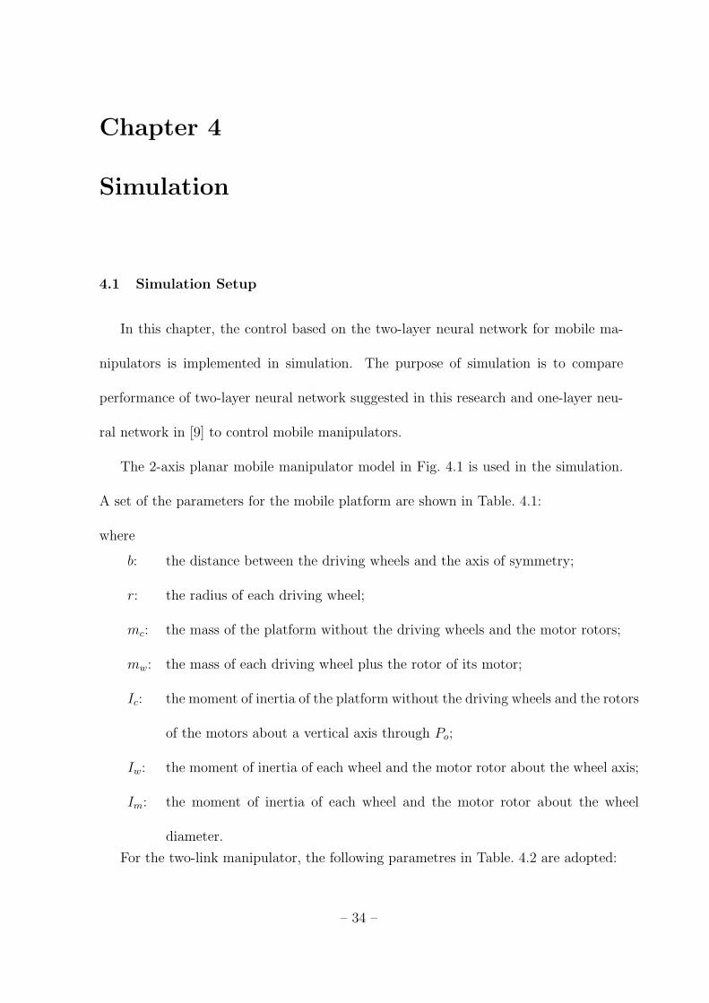
The 2-axis planar mobile manipulator model in Fig. 4.1 is used in the simulation.
A set of the parameters for the mobile platform are shown in Table. 4.1:
where
b: the distance between the driving wheels and the axis of symmetry;
r: the radius of each driving wheel;
mc: the mass of the platform without the driving wheels and the motor rotors;
mw: the mass of each driving wheel plus the rotor of its motor;
Ic: the moment of inertia of the platform without the driving wheels and the rotors
of the motors about a vertical axis through Po;
Iw: the moment of inertia of each wheel and the motor rotor about the wheel axis;
Im: the moment of inertia of each wheel and the motor rotor about the wheel
diameter.
For the two-link manipulator, the following parametres in Table. 4.2 are adopted:
– 34 –
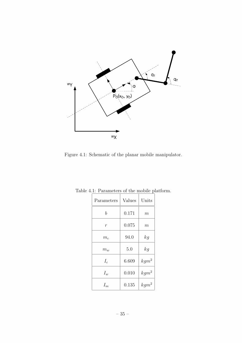
Figure 4.1: Schematic of the planar mobile manipulator.
Table 4.1: Parameters of the mobile platform.
Parameters Values Units
b 0.171 m
r 0.075 m
mc 94.0 kg
mw 5.0 kg
Ic 6.609 kgm2
Iw 0.010 kgm2
Im 0.135 kgm2
– 35 –
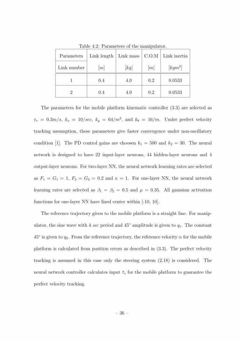
Table 4.2: Parameters of the manipulator.
Parameters Link length Link mass C.O.M Link inertia
Link number [m] [kg] [m] [kgm2]
1 0.4 4.0 0.2 0.0533
2 0.4 4.0 0.2 0.0533
The parameters for the mobile platform kinematic controller (3.3) are selected as
vr = 0.3m/s, kx = 10/sec, ky = 64/m2, and kθ = 16/m. Under perfect velocity
tracking assumption, these parameters give faster convergence under non-oscillatory
condition [1]. The PD control gains are choosen k1 = 500 and k2 = 30. The neural
network is designed to have 22 input-layer neurons, 44 hidden-layer neurons and 4
output-layer neurons. For two-layer NN, the neural network learning rates are selected
as F1 = G1 = 1, F2 = G2 = 0.2 and κ = 1. For one-layer NN, the neural network
learning rates are selected as β1 = β2 = 0.5 and µ = 0.35. All gaussian activation
functions for one-layer NN have fixed center within [-10, 10].
The reference trajectory given to the mobile platform is a straight line. For manip-
ulator, the sine wave with 4 sec period and 45◦ amplitude is given to q1. The constant
45◦ is given to q2. From the reference trajectory, the reference velocity α for the mobile
platform is calculated from position errors as described in (3.3). The perfect velocity
tracking is assumed in this case only the steering system (2.18) is considered. The
neural network controller calculates input τv for the mobile platform to guarantee the
perfect velocity tracking.
– 36 –
4.2 Simulation Results
The perfect velocity tracking assumption is made in this paper to convert steering
system inputs into actual vehicle commands. The simulation result of the control
designed based on this assumption is shown in this section. In the neural network
control, the neural network is added to the PD controller to compensate nonlinear and
coupled dynamics.
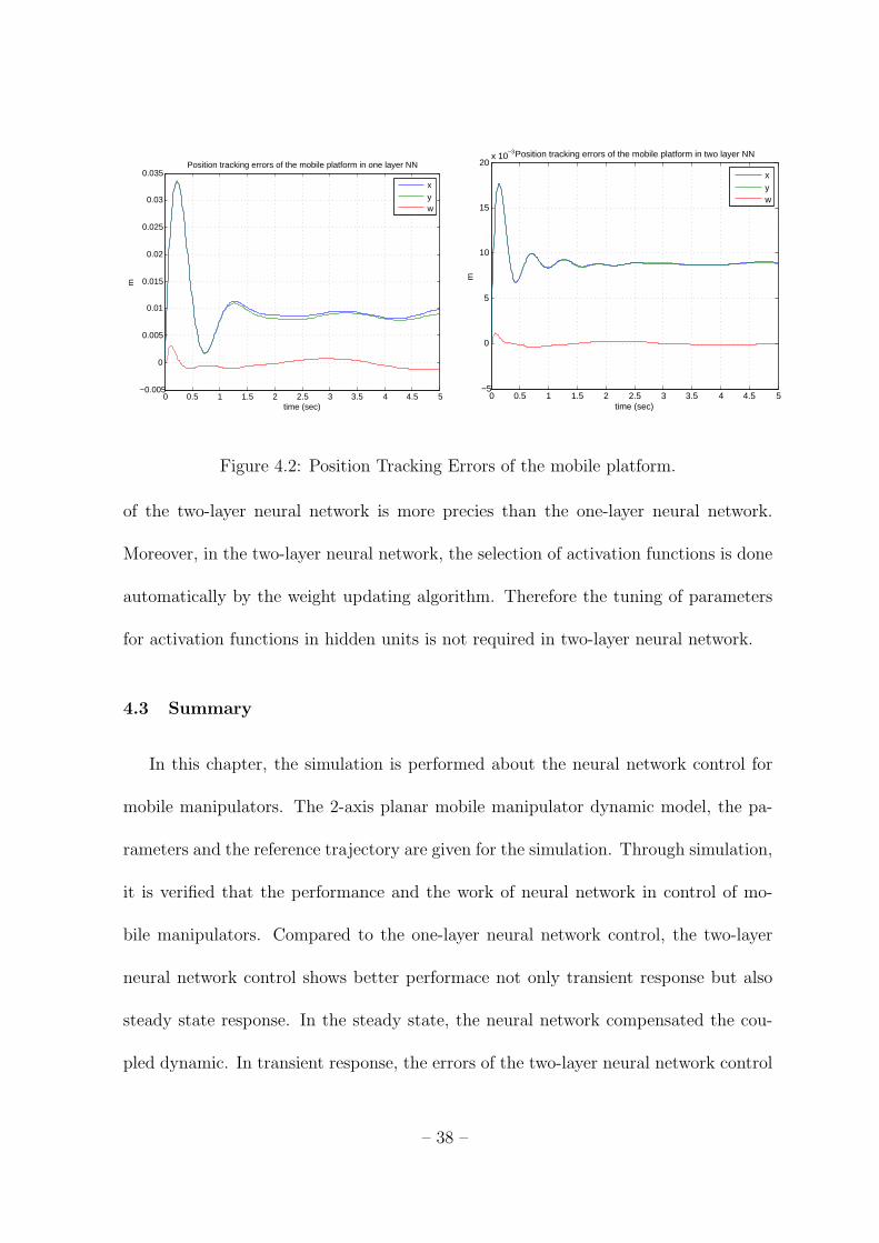
Fig. 4.2 shows the position tracking errors of the mobile platform in given trajectory.
The two-layer neural network control shows less transient and steady-state errors then
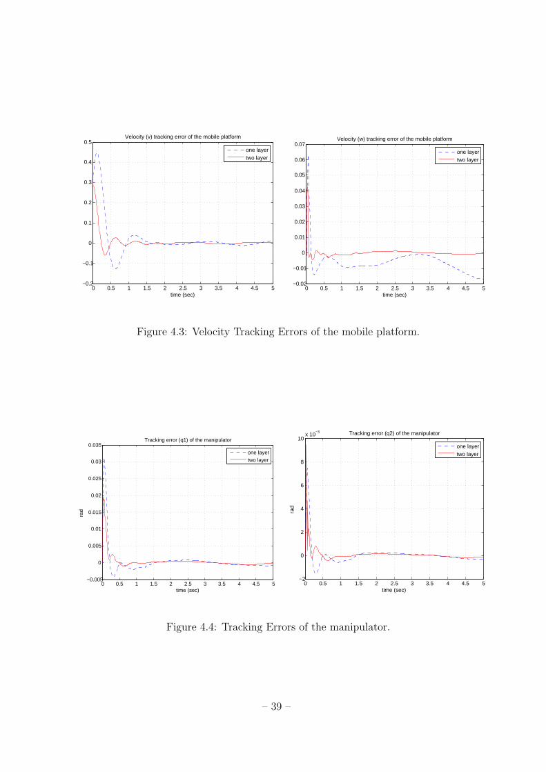
the one-layer neural network control. Fig. 4.3 represents the velocity tracking error z
of the mobile platform. The errors in v, w of the mobile platform are reduced after
the time elapsed because of the compensation of nonlinear and coupled dynamics by
the neural network. However the errors are arose intermittently in the influence of the
manipulator movement and the modeling errors of the neural network. In the case
of one-layer neural network, there are more tracking errors than the two-layer neural
network due to the more modeling errors in the neural network. Fig. 4.4 represents
the position tracking errors of the manipulator. In the initial time, there exist large
tracking error because there exist modelling errors. After learning process, the dynamic
model is estimated so the tracking error is decreased. The two-layer neural network
control shows better results than one-layer neural network control.
The two-layer neural network control shows the better performance with respect
to the one-layer neural network control. The performances like convergence time and
tracking errors are improved. Through the results, it is expected that the estimation
– 37 –
0 0.5 1 1.5 2 2.5 3 3.5 4 4.5 5−0.005
0
0.005
0.01
0.015
0.02
0.025
0.03
0.035
time (sec)
m
Position tracking errors of the mobile platform in one layer NN
xyw
0 0.5 1 1.5 2 2.5 3 3.5 4 4.5 5−5
0
5
10
15
20x 10
−3
time (sec)
m
Position tracking errors of the mobile platform in two layer NN
xyw
Figure 4.2: Position Tracking Errors of the mobile platform.
of the two-layer neural network is more precies than the one-layer neural network.
Moreover, in the two-layer neural network, the selection of activation functions is done
automatically by the weight updating algorithm. Therefore the tuning of parameters
for activation functions in hidden units is not required in two-layer neural network.
4.3 Summary
In this chapter, the simulation is performed about the neural network control for
mobile manipulators. The 2-axis planar mobile manipulator dynamic model, the pa-
rameters and the reference trajectory are given for the simulation. Through simulation,
it is verified that the performance and the work of neural network in control of mo-
bile manipulators. Compared to the one-layer neural network control, the two-layer
neural network control shows better performace not only transient response but also
steady state response. In the steady state, the neural network compensated the cou-
pled dynamic. In transient response, the errors of the two-layer neural network control
– 38 –
0 0.5 1 1.5 2 2.5 3 3.5 4 4.5 5−0.2
−0.1
0
0.1
0.2
0.3
0.4
0.5
time (sec)
Velocity (v) tracking error of the mobile platform
one layertwo layer
0 0.5 1 1.5 2 2.5 3 3.5 4 4.5 5−0.02
−0.01
0
0.01
0.02
0.03
0.04
0.05
0.06
0.07
time (sec)
Velocity (w) tracking error of the mobile platform
one layertwo layer
Figure 4.3: Velocity Tracking Errors of the mobile platform.
0 0.5 1 1.5 2 2.5 3 3.5 4 4.5 5−0.005
0
0.005
0.01
0.015
0.02
0.025
0.03
0.035
time (sec)
rad
Tracking error (q1) of the manipulator
one layertwo layer
0 0.5 1 1.5 2 2.5 3 3.5 4 4.5 5−2
0
2
4
6
8
10x 10
−3
time (sec)
rad
Tracking error (q2) of the manipulator
one layertwo layer
Figure 4.4: Tracking Errors of the manipulator.
– 39 –
are reduced faster than the one-layer neural network control. Moreover, due to the
weight updating algorithm in input-layer, the selection of activation functions is done
automatically in two-layer neural network. Therefore more reliable approximation is
expected.
– 40 –
Chapter 5
Experiments
5.1 Experiment Setup
The experiments are performed on the 2-axis planar manipulator on Fig. 5.1. The
dynamic parameters of the manipulator are assumed to be completely unknown. Each
joint is actuated by brushed DC motor and the joint angles are measured by encorder.
The angular velocity of joints is estimated by simple numerical position differentia-
tion, which caused significant estimation errors, and therefore, affected the control
performance. In addition, firction and backlash present in the joints were found to
have a significant influence on the tracking performance, and also greatly substanti-
ated the difficulty of control design. Even though the 2-axis planar manipulator has
relatively simple sturucture than mobile manipulators, the 2-axis planar manipulaotr
also presents a nonlinear and tightly coupled dynamics. Therefore the experiments on
this platform can also show the ability of neural network that can control a nonlinear
and tightly coupled dynamics.
Experiment configuration is shown in Fig. 5.2. DSP 2812 processor works as a
main controller. DSP 2812 is suitable for control application due to its high speed and
spherical devices like QEP, PWM and ADC modules. QEP modules treat encorder
signal to calculate joint angle, PWM modules output the control signal and ADC
– 41 –
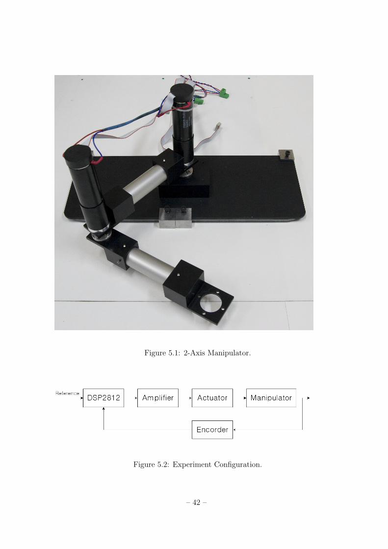
Figure 5.1: 2-Axis Manipulator.
Figure 5.2: Experiment Configuration.
– 42 –
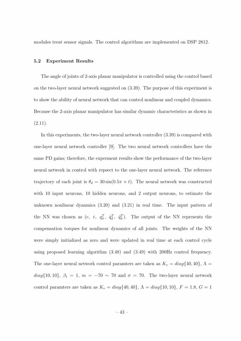
modules treat sensor signals. The control algorithms are implemented on DSP 2812.
5.2 Experiment Results
The angle of joints of 2-axis planar manipulator is controlled using the control based
on the two-layer neural network suggested on (3.39). The purpose of this experiment is
to show the ability of neural network that can control nonlinear and coupled dynamics.
Because the 2-axis planar manipulator has similar dynamic characteristics as shown in
(2.11).
In this experiments, the two-layer neural network controller (3.39) is compared with
one-layer neural network controller [9]. The two neural network controllers have the
same PD gains; therefore, the experment results show the performance of the two-layer
neural network in control with repsect to the one-layer neural network. The reference
trajectory of each joint is θd = 30 sin(0.5π × t). The neural network was constructed
with 10 input neurons, 10 hidden neurons, and 2 output neurons, to estimate the
unknown nonlinear dyanmics (3.20) and (3.21) in real time. The input pattern of
the NN was chosen as (e, e, qTd , qTd , q
Td ). The output of the NN represents the
compensation torques for nonlinear dynamics of all joints. The weights of the NN
were simply initialized as zero and were updated in real time at each control cycle
using proposed learning algorithm (3.48) and (3.49) with 200Hz control frequency.
The one-layer neural network control paramters are taken as Kv = diag{40, 40}, Λ =
diag{10, 10}, β1 = 1, m = −70 ∼ 70 and σ = 70. The two-layer neural network
control paramters are taken as Kv = diag{40, 40}, Λ = diag{10, 10}, F = 1.8, G = 1
– 43 –
and κ = 0.007.
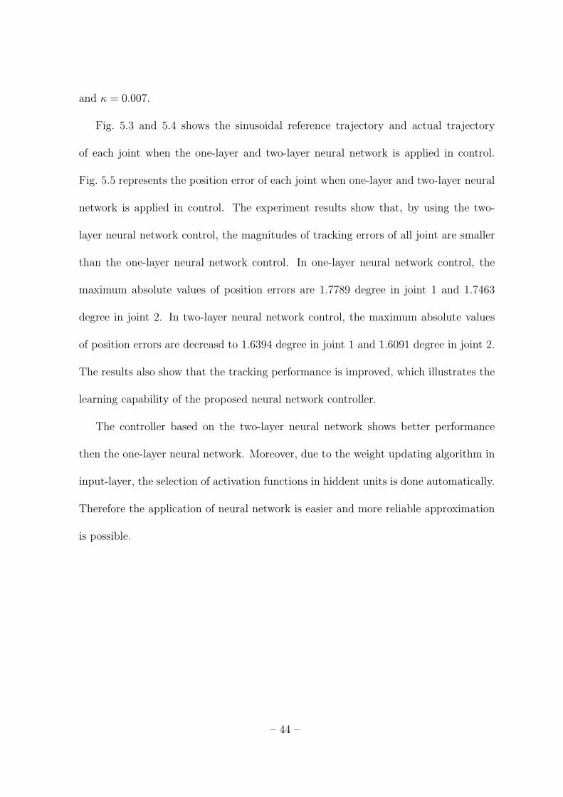
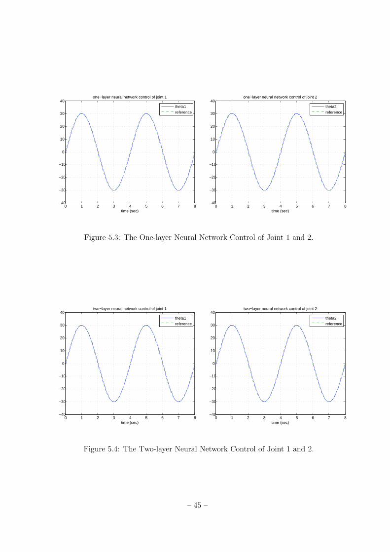
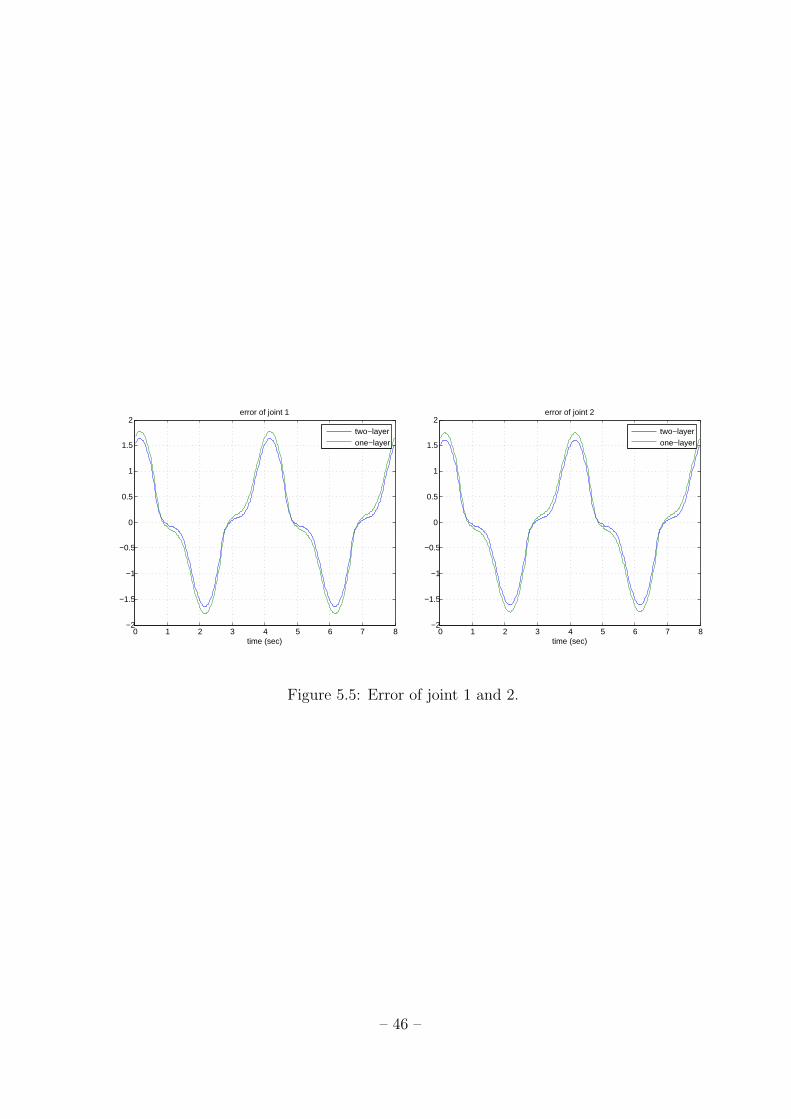
Fig. 5.3 and 5.4 shows the sinusoidal reference trajectory and actual trajectory
of each joint when the one-layer and two-layer neural network is applied in control.
Fig. 5.5 represents the position error of each joint when one-layer and two-layer neural
network is applied in control. The experiment results show that, by using the two-
layer neural network control, the magnitudes of tracking errors of all joint are smaller
than the one-layer neural network control. In one-layer neural network control, the
maximum absolute values of position errors are 1.7789 degree in joint 1 and 1.7463
degree in joint 2. In two-layer neural network control, the maximum absolute values
of position errors are decreasd to 1.6394 degree in joint 1 and 1.6091 degree in joint 2.
The results also show that the tracking performance is improved, which illustrates the
learning capability of the proposed neural network controller.
The controller based on the two-layer neural network shows better performance
then the one-layer neural network. Moreover, due to the weight updating algorithm in
input-layer, the selection of activation functions in hiddent units is done automatically.
Therefore the application of neural network is easier and more reliable approximation
is possible.
– 44 –
0 1 2 3 4 5 6 7 8−40
−30
−20
−10
0
10
20
30
40
time (sec)
one−layer neural network control of joint 1
theta1reference
0 1 2 3 4 5 6 7 8−40
−30
−20
−10
0
10
20
30
40
time (sec)
one−layer neural network control of joint 2
theta2reference
Figure 5.3: The One-layer Neural Network Control of Joint 1 and 2.
0 1 2 3 4 5 6 7 8−40
−30
−20
−10
0
10
20
30
40
time (sec)
two−layer neural network control of joint 1
theta1reference
0 1 2 3 4 5 6 7 8−40
−30
−20
−10
0
10
20
30
40
time (sec)
two−layer neural network control of joint 2
theta2reference
Figure 5.4: The Two-layer Neural Network Control of Joint 1 and 2.
– 45 –
0 1 2 3 4 5 6 7 8−2
−1.5
−1
−0.5
0
0.5
1
1.5
2
time (sec)
error of joint 1
two−layerone−layer
0 1 2 3 4 5 6 7 8−2
−1.5
−1
−0.5
0
0.5
1
1.5
2
time (sec)
error of joint 2
two−layerone−layer
Figure 5.5: Error of joint 1 and 2.
– 46 –
Chapter 6
Conclusion and Future Work
Controlling a mobile manipulator is difficult because of its structural complexity
arise from combining the manipulator and the mobile platform like redundancy, non-
holonomic constraints, and nonlinear dynamics with dynamic interaction of the ma-
nipulator and the mobile platform. This study mainly focuses on the nonholonomic
constraints and the nonlinear dynamics with dynamic interaction.
In this thesis, the control for mobile manipulators is suggested based on the two-
layer neural network. This neural network requires no preselection of the basis set. In
effect, by the weight updating algorithm for first-layer, the neural network can learn
its own basis set for the system nonlinearities. Therefore, by the weight updating algo-
rithm for first-layer, the activation functions corresponding to the basis set is selected
automatically. Also more precise estimation of a function can be expected. Thus, the
main contribution of this thesis is to improve the performance of the neural network
of [9] by enhancing the weight updating mechanism.
In chapter 2, the dynamic model of mobile manipulators is represented including
nonholonomic constraints and nonlinear dynamics with dynamic interaction. Moreover,
the nonholonomic constraint in the mobile platform is defined and analyzed.
In chapter 3, the control structure for mobile manipulators is represented. The
problems like nonholonomic constraints and nonlinear dynamics with dynamic inter-
– 47 –
action between the mobile platform and the manipulator is considered. Moreover, the
control algorithm τv and τr based on two-layer neural network with the weight up-
dating algorithm are derived. The tracking stability of the closed-loop system, the
convergence of the neural network weight-updating process and boundedness of of the
neural network weight estimation errors are all guaranteed through Lyapunov function.
In chapter 4, the control with the two-layer neural network is implemented in the
simulation. The control using two-layer neural network is compared with one-layer
neural network. The control based on the two-layer neural network shows better per-
formance in transient and steady-state resonse. In chapter 5, the control with the
two-layer neural network is used to cotrol the 2-axis manipulator. The control based
on the two-layer neural network shows better performance than the one-layer neural
network. The two-layer neural network selects the activation functions automatically
by the input-layer update with the weight updating algorithm. The number of param-
eters requiring tuning is reduced; thus the application of the neural network is easier
and a more precise estimation have been achieved.
– 48 –
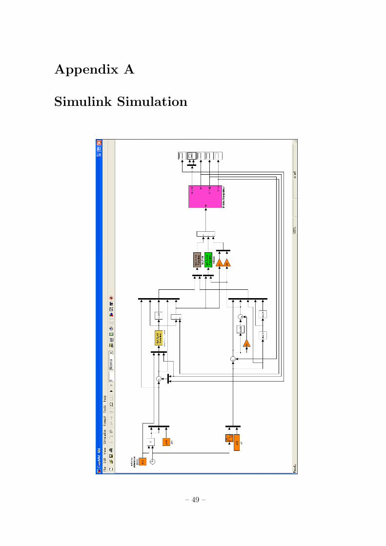
Appendix A
Simulink Simulation
– 49 –
Appendix B
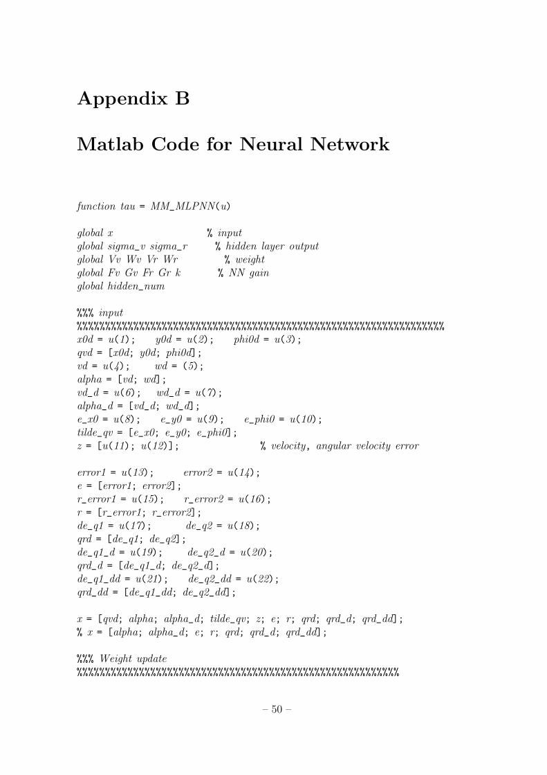
Matlab Code for Neural Network
function tau = MM_MLPNN(u)
global x % inputglobal sigma_v sigma_r % hidden layer outputglobal Vv Wv Vr Wr % weightglobal Fv Gv Fr Gr k % NN gainglobal hidden_num
%%% input%%%%%%%%%%%%%%%%%%%%%%%%%%%%%%%%%%%%%%%%%%%%%%%%%%%%%%%%%%%%%%%%%
x0d = u(1); y0d = u(2); phi0d = u(3);qvd = [x0d; y0d; phi0d];vd = u(4); wd = (5);alpha = [vd; wd];vd_d = u(6); wd_d = u(7);alpha_d = [vd_d; wd_d];e_x0 = u(8); e_y0 = u(9); e_phi0 = u(10);tilde_qv = [e_x0; e_y0; e_phi0];z = [u(11); u(12)]; % velocity, angular velocity error
error1 = u(13); error2 = u(14);e = [error1; error2];r_error1 = u(15); r_error2 = u(16);r = [r_error1; r_error2];de_q1 = u(17); de_q2 = u(18);qrd = [de_q1; de_q2];de_q1_d = u(19); de_q2_d = u(20);qrd_d = [de_q1_d; de_q2_d];de_q1_dd = u(21); de_q2_dd = u(22);qrd_dd = [de_q1_dd; de_q2_dd];
x = [qvd; alpha; alpha_d; tilde_qv; z; e; r; qrd; qrd_d; qrd_dd];% x = [alpha; alpha_d; e; r; qrd; qrd_d; qrd_dd];
%%% Weight update%%%%%%%%%%%%%%%%%%%%%%%%%%%%%%%%%%%%%%%%%%%%%%%%%%%%%%%%%
– 50 –
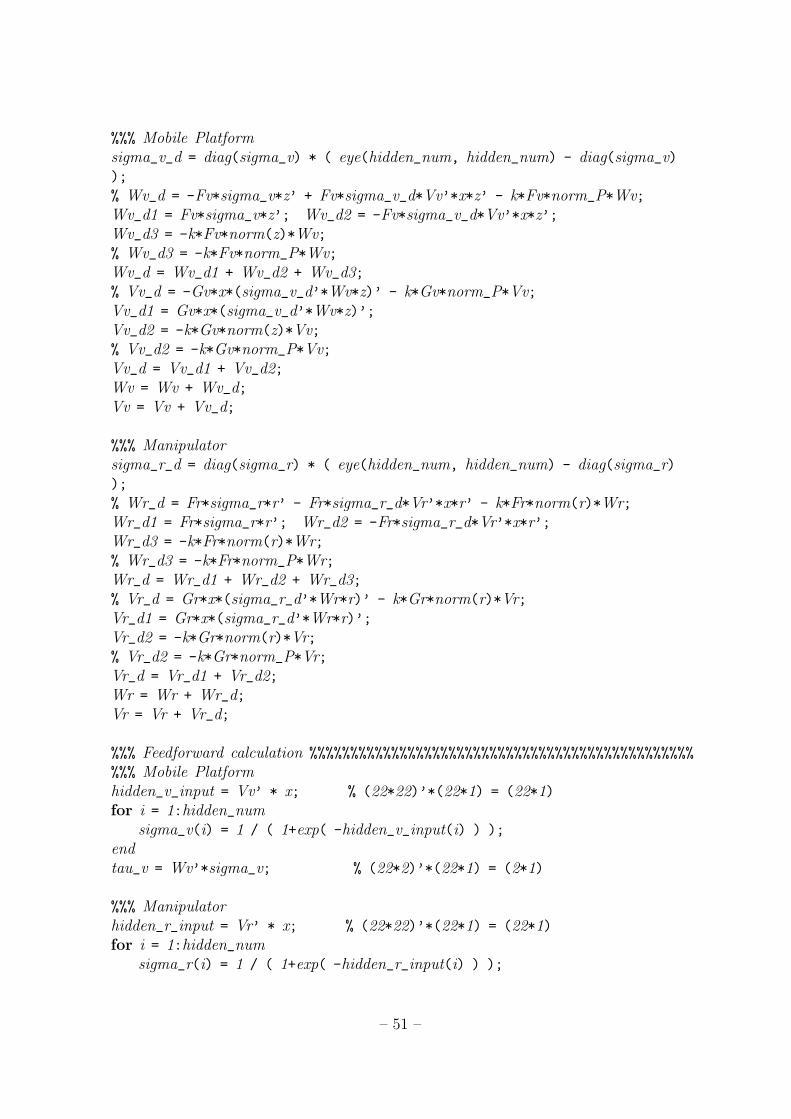
%%% Mobile Platformsigma_v_d = diag(sigma_v) * ( eye(hidden_num, hidden_num) - diag(sigma_v));
% Wv_d = -Fv*sigma_v*z’ + Fv*sigma_v_d*Vv’*x*z’ - k*Fv*norm_P*Wv;Wv_d1 = Fv*sigma_v*z’; Wv_d2 = -Fv*sigma_v_d*Vv’*x*z’;Wv_d3 = -k*Fv*norm(z)*Wv;% Wv_d3 = -k*Fv*norm_P*Wv;Wv_d = Wv_d1 + Wv_d2 + Wv_d3;% Vv_d = -Gv*x*(sigma_v_d’*Wv*z)’ - k*Gv*norm_P*Vv;Vv_d1 = Gv*x*(sigma_v_d’*Wv*z)’;Vv_d2 = -k*Gv*norm(z)*Vv;% Vv_d2 = -k*Gv*norm_P*Vv;Vv_d = Vv_d1 + Vv_d2;Wv = Wv + Wv_d;Vv = Vv + Vv_d;
%%% Manipulatorsigma_r_d = diag(sigma_r) * ( eye(hidden_num, hidden_num) - diag(sigma_r));
% Wr_d = Fr*sigma_r*r’ - Fr*sigma_r_d*Vr’*x*r’ - k*Fr*norm(r)*Wr;Wr_d1 = Fr*sigma_r*r’; Wr_d2 = -Fr*sigma_r_d*Vr’*x*r’;Wr_d3 = -k*Fr*norm(r)*Wr;% Wr_d3 = -k*Fr*norm_P*Wr;Wr_d = Wr_d1 + Wr_d2 + Wr_d3;% Vr_d = Gr*x*(sigma_r_d’*Wr*r)’ - k*Gr*norm(r)*Vr;Vr_d1 = Gr*x*(sigma_r_d’*Wr*r)’;Vr_d2 = -k*Gr*norm(r)*Vr;% Vr_d2 = -k*Gr*norm_P*Vr;Vr_d = Vr_d1 + Vr_d2;Wr = Wr + Wr_d;Vr = Vr + Vr_d;
%%% Feedforward calculation %%%%%%%%%%%%%%%%%%%%%%%%%%%%%%%%%%%%%%%%%%%%%%%
%%% Mobile Platformhidden_v_input = Vv’ * x; % (22*22)’*(22*1) = (22*1)for i = 1:hidden_num
sigma_v(i) = 1 / ( 1+exp( -hidden_v_input(i) ) );
endtau_v = Wv’*sigma_v; % (22*2)’*(22*1) = (2*1)
%%% Manipulatorhidden_r_input = Vr’ * x; % (22*22)’*(22*1) = (22*1)for i = 1:hidden_num
sigma_r(i) = 1 / ( 1+exp( -hidden_r_input(i) ) );
– 51 –
endtau_r = Wr’*sigma_r; % (22*2)’*(22*1) = (2*1)
tau = [tau_v; tau_r];
– 52 –
References
1. Y. Kanayama, Y. Kimura, F. Miyazaki and T. Noguchi, A Stable tracking control
method for an autonomous mobile robot. Proc. IEEE Conf. Robot. Automat., vol.
1, pp. 384-389, 1990.
2. R. Fierro and F. L. Lewis, Control of a nonholonomic mobile robot using neural
networks. Proc. IEEE Trans. Robot. Automat., vol. 9, pp. 589-600, 1998.
3. Y. Li and A. A. Frank, A moving base robot. Proc, of 1986 American Control
Conference, pages 1927-1932, 1986.
4. S. Dubowsky and A. B. Tanner, A study of the dyanmics and control of mobile
manipulators subjected to vehicle disturbances. Proc. 4th International symposium
of Robotics Research, pages 111-117, 1987
5. K. Liu and F. L. Lewis, Decentralized continuous robust controller for mobile
robots. Proc. IEEE Conf. Robot. Automat., pp.1822-1827, 1990.
6. N. A. M. Hootsmans, The Motion Control of Manipulators on Mobile Vehicles.
PhD thesis, Department of Mechanical Engineering, MIT, Cambridge, 1992
7. Y. Yamamoto, Modelling and control of mobile manipulators. Ph.D. dissertation,
Univ. Michigan, Ann Arbor, 1994.
8. J. Chung, S. Velinsky, and R. Hess, Interaction control of a redundant mobile
manipulator. Int. J. Robot. Res., vol. 17, no. 12, pp. 1302-1309, 1998.
– 53 –
9. Sheng Lin and A. A. Goldenberg, Neural-Network Control of Mobile Manipulators.
IEEE Trans. Neural Netw., vol. 12, no. 5, pp. 1121-1133, 2001.
10. Wenjie Dong, On trajectory and force tracking control of constrained mobile
manipulators with parameter uncertainty. automatica., vol. 38, pp. 1475-1484,
2002.
11. Z. P. Wang, S. S. Ge and T. H. Lee, Robust Motion/Force Control of Uncertain
Holonomic/Nonholonomic Mechanical Systems. IEEE/ASME Trans. Mechatron-
ics., vol. 38, pp. 1475-1484, 2004.
12. Zhijun Li, Shuzhi Sam Ge and Aiguo Ming, Adaptive Robust Motion/Force Con-
trol of Holonomic-Constrained Nohholonomic Mobile Manipulators. IEEE Trans.
System, man, and cybernetics., vol. 37, pp. 607-616, 2007.
13. Chunyan Gao, Minglu Zhang and Ruisi Liu, Research on the Method and Exper-
iment of the coordinated Control for Wheeled mobile manipulaotrs. In proceeding
of IEEE International Conference on Automation and Logistics., pp. 2386-2390,
2008.
14. Glenn D. White, Rejankumar M. Bhatt and Chin Pei Tang, Experiment Evalua-
tion of Dynamic Redundancy Resolution in a Nonholonomic wheeled Mobile Ma-
nipulator. IEEE/ASME Trans. Mechatronics., vol. 14, No. 3, pp. 349-357, 2009.
15. Yasuhisa Hirata, Youhei Kume, Zhi-dong Wang and Kazuhiro Kosuge, Handling
of a Single Object by Multiple Mobile Manipulators in cooperation with Human.
JSME Internatinal journal., Series C, vol. 48, No. 4, pp. 613-619, 2005.
– 54 –
16. F. L. Lewis, S. Jagannathan, and A. Yesildirek, Neural Network Control of Robot
Manipulators and Nonlineaer Systems. London, U.K.: Taylor and Francis, 1999.
17. O. Khatib et al, Vehicle/arm coordination and multiple mobile manipulator de-
centralized cooperation. Proc. IEEE/RSJ Conf. Intell. Root. Syst., vol. 3, 1996.
18. Richard M. Murray, Zexiang Li, S. Shankar Sastry, A mathmatical Introduction
to ROBOTIC MANIPULATION. CRC Press, 1994.
19. Mark W. Spong, Seth Hutchison and M. Vidyasagar, ROBOT MODELING AND
CONTROL. John Wiley & Sons, Inc., 2006.
– 55 –