Implementation of quantum imaginary-time evolution method on NISQ devices:Nonlocal approximation

Hirofumi Nishi, Taichi Kosugi, and Yu-ichiro MatsushitaLaboratory for Materials and Structures, Institute of Innovative Research,

Tokyo Institute of Technology, Tokyo, 152-8550, Japan.Quemix Inc., Tokyo, 103-0027, Japan.

(Dated: May 27, 2020)

The imaginary-time evolution method is widely known to be efficient for obtaining the groundstate in quantum many-body problems on a classical computer. A recently proposed quantumimaginary-time evolution method (QITE) faces problems of deep circuit depth and difficulty in theimplementation on noisy intermediate-scale quantum (NISQ) devices. In this study, a nonlocal ap-proximation is developed to tackle this difficulty. We found that by removing the locality conditionor local approximation (LA), which was imposed when the imaginary-time evolution operator isconverted to a unitary operator, the quantum circuit depth is significantly reduced. We proposetwo-step approximation methods based on a nonlocality condition: extended LA (eLA) and nonlo-cal approximation (NLA). To confirm the validity of eLA and NLA, we apply them to the max-cutproblem of an unweighted 3-regular graph and a weighted fully connected graph; we comparativelyevaluate the performances of LA, eLA, and NLA. The eLA and NLA methods require far fewercircuit depths than LA to maintain the same level of computational accuracy. Further, we devel-oped a “compression” method of the quantum circuit for the imaginary-time steps as a method tofurther reduce the circuit depth in the QITE method. The eLA, NLA, and the compression methodintroduced in this study allow us to reduce the circuit depth and the accumulation of error causedby the gate operation significantly and pave the way for implementing the QITE method on NISQdevices.

Quantum computers, initially proposed byFeynmann[1], were unveiled by Deutsch[2], Grover[3],and Shor[4] to have great potential that could overwhelm-ingly surpasses classical computers. In addition, thenews of Google’s demonstration of quantum supremacyin 2019 has spread around the world[5] and expectationsfor the realization of practical quantum computers areincreasing. One of the most promising problems forquantum computers is combinatorial optimization, whichis a NP-hard problem[6]. Combinatorial optimizationproblems are closely related to our daily lives, and theyinclude the traveling salesman problem[7], schedulingproblem[8], SAT (satisfiability problem) solver[9], amongothers. For these combinatorial optimization problems,Grover’s algorithm is already known to improve thecomputational cost with quadratic speedup compared toclassical computers[10, 11].

Under these circumstances, it is challenging for re-searchers all over the world to employ existing ornear-future quantum computers to achieve tasks thatare very difficult or impossible using classical comput-ers. Currently available quantum computers are noisyintermediate-scale quantum (NISQ) devices[12]. Further,conventional quantum algorithms require many gate op-erations, such as Grover’s algorithm, and they cannot beimplemented on NISQ devices with no error correctionand short coherence time. Recently, classical-quantumhybrid algorithms called variational quantum eigensolver(VQE)[13, 14], and quantum approximate optimizationalgorithm (QAOA)[15–20] have been proposed for NISQdevices. In these methods, ansatz states with parame-ters are implemented as quantum circuits, and the pa-rameters included in the ansatz states are optimized on

a classical computer. While VQE and QAOA can berealized with a limited number of quantum operationsand have good noise tolerance, it is difficult to determinethe ansatz states properly and converge high-dimensionalparameters[21].

For quantum many-body problems, an imaginary-timeevolution method is a known computational method toidentify the ground state. The imaginary-time evolutionmethod selectively extracts the ground state componentby performing time evolution in the direction of imagi-nary time. Various combinatorial optimization problemsare converted to a Hamiltonian format, and their corre-sponding Hamiltonian is derived[22]. Thus, it is possibleto solve the combinatorial optimization problem usingthe imaginary-time evolution method.

The implementation of the imaginary-time evolutionmethod on a quantum computer involves a critical prob-lem in that the imaginary-time evolution operator is anonunitary operator, and therefore, it cannot implementthe imaginary-time evolution method on a quantum com-puter in its current state. To overcome this challenge, twoimaginary-time evolution methods— one that assumes anansatz state and another that does not—were proposedin this study. The method that assumes the ansatz statetraces the imaginary-time evolution of the parameterscontained in the ansatz state[23–25]. The other methodintroduces a unitary operation to reproduce the state onwhich the imaginary-time evolution operator has actedaccurately[26–28]. The latter quantum imaginary-timeevolution (QITE) method is considered an efficient ap-proach to the optimization problem because it does notneed to assume an ansatz state; further, there is no prob-lem of convergence of high-dimensional parameters, even

arX

iv:2

005.

1271

5v1

[qu

ant-

ph]

26

May

202

0

2

when compared to QAOA.We focus on the QITE method without the ansatz

assumption and apply it to the optimization problems.The QITE method proposed in the previous researchhas problems with circuit depth and computational cost;even a simple one-dimensional Ising model requires 44 =256 fourth-order tensor-product operators[26]. Further,more complex problems are challenging to implement onNISQ devices.

Therefore, we propose two approximations and onecomputational technique to overcome this difficulty. Wesucceeded in significantly reducing the quantum circuitdepth of the QITE method, and we applied the devel-oped algorithms to the max-cut problem, which is anNP-hard problem. For the max-cut problem, we chosean unweighted 3-regular graph and a weighted fully con-nected graph. The latter is a problem known as the clas-sification problem in the context of unsupervised machinelearning[29, 30].

METHOD

Unitarization of imaginary-time evolution operators

Consider a scenario wherein a Hamiltonian H is givenfor the optimization problem considered in this study.The Hamiltonian H is expressed as the summation of

some partial Hamiltonians h[m] as H =∑Nham

m=1 h[m],where Nham is the number of the partial Hamiltonians.The max-cut problem, which is a computational target ofthis work, is represented by the Hamiltonian in the formof Ising spins and can be mapped to the Pauli operatorrepresentation for qubits in a straightforward manner. Inthe case of the Hamiltonian of quantum chemistry, eachpartial Hamiltonian can be mapped to the Pauli-operatorrepresentation on qubits via the Bravyi–Kitaev represen-tation [31] or Jordan–Wigner representation [32].

For a given Hamiltonian, the ground state is obtainedby using the imaginary-time evolution method. We apply

the imaginary-time evolution operator defined by e−τH ,where τ is the imaginary time to reach the initial (τ = 0)

state of the system, |Ψ(τ = 0)〉; and e−τH |Ψ(τ = 0)〉.The imaginary-time evolution operator is decomposed bya first-order Suzuki–Trotter decomposition into ones witha small imaginary-time step ∆τ (τ ≡ ∆τ ×Nstep) of the

individual partial Hamiltonians h[m].

e−τH =

Nstep∏n=1

Nham∏m=1

e−∆τh[m] +O(∆τ2) .

Because the operators of the imaginary-time evolutionare nonunitary, they cannot be directly implemented asa gate operation on a quantum computer. In the QITE

method, the unitary operator e−i∆τAn[m] is defined such

that it reproduces the state e−∆τH |Ψn〉 for a given state

|Ψn〉 ≡ |Ψ(τ = n∆τ)〉. We determine the Hermitian op-

erator An[m] that minimizes the following residual norm.∥∥∥∥∥∥ e−∆τh[m]|Ψn〉√〈Ψn|e−2∆τh[m]|Ψn〉

− e−i∆τAn[m]|Ψn〉

∥∥∥∥∥∥2

. (1)

Nonlocal condition for imaginary-time evolutionoperators

We express the Hermitian operator An[m] as a linearcombination of the D-th order tensor products of Paulioperators {Il, σX,l, σY,l, σZ,l} acting on the l-th qubit as

An[m] =∑

lk+1,··· ,lD∈Lm

′ ∑i1···iD

a(n)i1···iD,l1···lD [m]

σi1,l1(m) ⊗ · · · ⊗ σiD,lD ,(2)

where the prime on the first summation symbol indi-cates removing the double counting of the repeated ten-sors. We defined Lm as the set of NLm qubits, eachof which interact with those in the partial Hamiltonian

h[m]; however, it is not contained in h[m]. The pa-rameter D, which is called the domain size, satisfiesk 5 D 5 k+NLm , where we assumed the partial Hamil-

tonian h[m] to be written by a tensor product of thek-th order. {l1(m), · · · , lk(m)} is the set of qubits con-

tained in the partial Hamiltonian h[m]. The summationin Eq. (2) is taken over all combinations of D−k qubits,{lk+1(m), · · · , lD(m)}, and chosen from Lm. D is an in-put parameter that represents the level of approximation;a larger D indicates that the imaginary-time evolutionoperator is expressed using higher-order tensor productsand the residual norm in Eq. (1) shows a smaller value,which leads to a better approximation. We consider ascenario where the domain size D incorporates all ele-ments in Lm, namely D = k + NLm

, and then Eq. (2)reproduces the operator An[m] introduced in Ref. [26].This implies that Eq. (2) is a natural extension of the ap-proximation introduced in Ref. [26]. We call the methodfor determining the operator An[m] defined in Ref. [26]local approximation (LA) for comparison with later ap-proximation. Then, we refer to the method defined in Eq.(2) as extended local-approximation (eLA). The follow-ing notation is used to indicate the domain size D: e.g.,LA with D = 6 is denoted by LA-D6. Note that, for LA,it is a well-defined approximation only when the domainsize D = k+NLm , and the value of D that can be taken islimited by the Hamiltonian. In addition, note that eLAcan remove such constraints on the Hamiltonian and flex-ibly determine the parameter D by considering the lin-ear combination for qubits. This flexibility is obvious inthe max-cut problem of the fully connected graph. Solv-ing the minimization problem in Eq. (1) to determine

the coefficients a(n){i,l}[m] results in the linear equation

S(n)a(n)[m] = b(n)[m], which can be solved using a classi-

cal computer. Here, S(n){i,li}{j,lj} = 〈Ψn|σ†{i,li}σ{j,lj}|Ψn〉

3

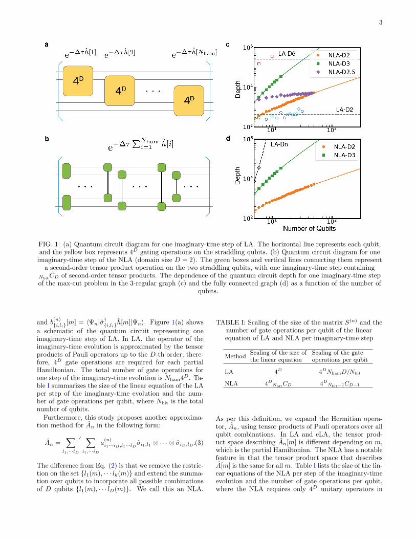
FIG. 1: (a) Quantum circuit diagram for one imaginary-time step of LA. The horizontal line represents each qubit,and the yellow box represents 4D gating operations on the straddling qubits. (b) Quantum circuit diagram for one

imaginary-time step of the NLA (domain size D = 2). The green boxes and vertical lines connecting them representa second-order tensor product operation on the two straddling qubits, with one imaginary-time step containing

NbitCD of second-order tensor products. The dependence of the quantum circuit depth for one imaginary-time step

of the max-cut problem in the 3-regular graph (c) and the fully connected graph (d) as a function of the number ofqubits.

and b(n){i,li}[m] = 〈Ψn|σ†{i,li}h[m]|Ψn〉. Figure 1(a) shows

a schematic of the quantum circuit representing oneimaginary-time step of LA. In LA, the operator of theimaginary-time evolution is approximated by the tensorproducts of Pauli operators up to the D-th order; there-fore, 4D gate operations are required for each partialHamiltonian. The total number of gate operations forone step of the imaginary-time evolution is Nham4D. Ta-ble I summarizes the size of the linear equation of the LAper step of the imaginary-time evolution and the num-ber of gate operations per qubit, where Nbit is the totalnumber of qubits.

Furthermore, this study proposes another approxima-tion method for An in the following form:

An =∑l1,···lD

′ ∑i1,···iD

a(n)i1···iD,l1···lD σi1,l1 ⊗ · · · ⊗ σiD,lD .(3)

The difference from Eq. (2) is that we remove the restric-tion on the set {l1(m), · · · lk(m)} and extend the summa-tion over qubits to incorporate all possible combinationsof D qubits {l1(m), · · · lD(m)}. We call this an NLA.

TABLE I: Scaling of the size of the matrix S(n) and thenumber of gate operations per qubit of the linearequation of LA and NLA per imaginary-time step

MethodScaling of the size ofthe linear equation

Scaling of the gateoperations per qubit

LA 4D 4DNhamD/Nbit

NLA 4DNbitCD 4D

Nbit−1CD−1

As per this definition, we expand the Hermitian opera-tor, An, using tensor products of Pauli operators over allqubit combinations. In LA and eLA, the tensor prod-uct space describing An[m] is different depending on m,which is the partial Hamiltonian. The NLA has a notablefeature in that the tensor product space that describesA[m] is the same for all m. Table I lists the size of the lin-ear equations of the NLA per step of the imaginary-timeevolution and the number of gate operations per qubit,where the NLA requires only 4D unitary operators in

4

NbitCD combinations for the quantum circuit in the first

step of the imaginary-time evolution. Figure 1(b) showsthe schematic of the quantum circuit of the NLA for onestep of the imaginary-time evolution (for D = 2).

RESULTS

To clarify the accuracy and effectiveness of NLA, weapplied it to the max-cut problem, which is an NP-hardproblem. The Hamiltonian of the max-cut problem inqubit representation is given in the following form con-taining second-order tensor products [22].

H = −∑

(i,j)∈E

di,j1− σZ,iσZ,j

2

As for the max-cut problem, we considered typical graphssuch as 3-regular and fully connected graphs. The 3-regular graphs have three connected edges at every ver-tex, where E is the set of edges contained in the graphand di,j is the weight of the edges connecting the ith andjth vertices.

Reduction effect of circuit depth

The circuit depths when LA and NLA are applied tothe max-cut problem are shown in Fig. 1(c) for the 3-regular graph and Fig. 1(d) for the fully-connected graphbecause different graphs of the max-cut problem changethe number of the partial Hamiltonian Nham; the neces-sary circuit depths for each approximation change cor-respondingly. In Fig. 1(c) and (d), the circuit depthcalculated using Qiskit[33] is plotted with points, andthe plotted points are extrapolated. In the case of k-regular graphs, the number of the partial Hamiltoniansis given by Nham = kNbit/2. It increases linearly withthe number of vertices Nbit so that the number of gateoperations per qubit does not depend on the number ofqubits, as listed in Table I. Thus, we extrapolated usingy = const.. In NLA, regardless of the structure of theHamiltonian, the number of gate operations per qubitis scaled by O(Nbit

D−1) with respect to the number ofqubits Nbit because all combinations of Nbit

CD are takenfor gate operations including the D-th order tensor prod-uct. In Figure 1(c), the circuit depth of the NLA is ex-trapolated by the function fitted by f(x) = xD−1.

Note that in LA, D = 3, 4, and 5 are not welldefined in the 3-regular graph. Thus, D = 6 is re-quired, and 46 = 4096 gate operations are necessary forthe imaginary-time evolution of one partial Hamiltonian,which leads to a deeper circuit depth and difficulty in im-plementation on NISQ devices. In addition, the circuitdepth required for LA-D6, compared to NLA-D2, NLA-D3, etc., is considerably higher in the region with a smallnumber of qubits. The circuit depth of the NLA becomesdeeper than that of LA in the region where the numberof qubits increases.

In Figure 1(d), LA-D2 and eLA-D3 are not shown forthe fully connected graph (Nham = Nbit

C2) because thecircuit depth of LA-D2 is equal to that of the NLA-D2,and that of eLA-D3 is equal to that of NLA-D3. In addi-tion, because the domain size has to be D = Nbit in LA,which is the exact imaginary-time evolution in a fullyconnected graph, and the circuit depth increases expo-nentially with respect to the number of qubits. In NLA,it can be scaled down to the linear or quadratic func-tion with respect to the number of qubits. This resultindicates that the NLA and eLA are efficient in reducingthe circuit depth, especially when the number of partialHamiltonians increases; further, these algorithms are ef-fective for NISQ devices.

Calculation accuracy

Simulations were performed after modifying the codeprovided in Ref. [26]. As an initial state, we adopted astate in which all states were superimposed with equal apriori weights. We adopt a figure of merit to discuss theaccuracy of the QITE method.

r = limτ→∞

〈Ψ(τ)|H|Ψ(τ)〉EGS

.

The first target of the max-cut problem is an un-weighted 3-regular graph with ten vertices, where EGS

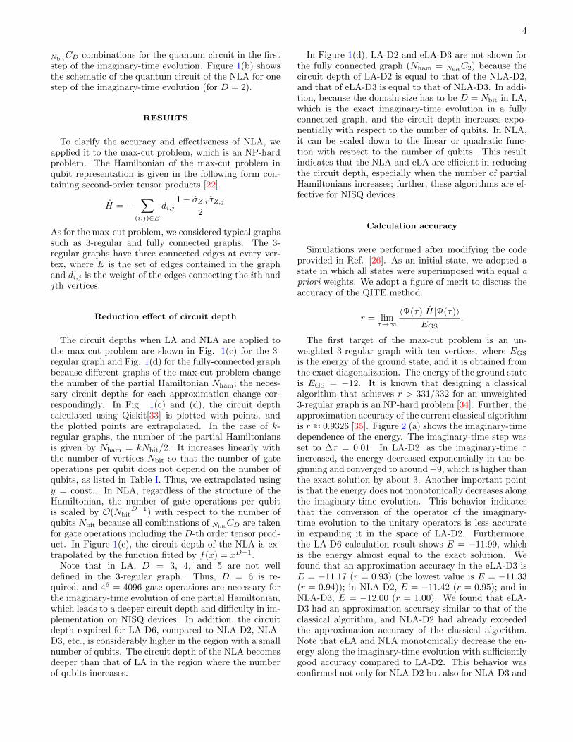
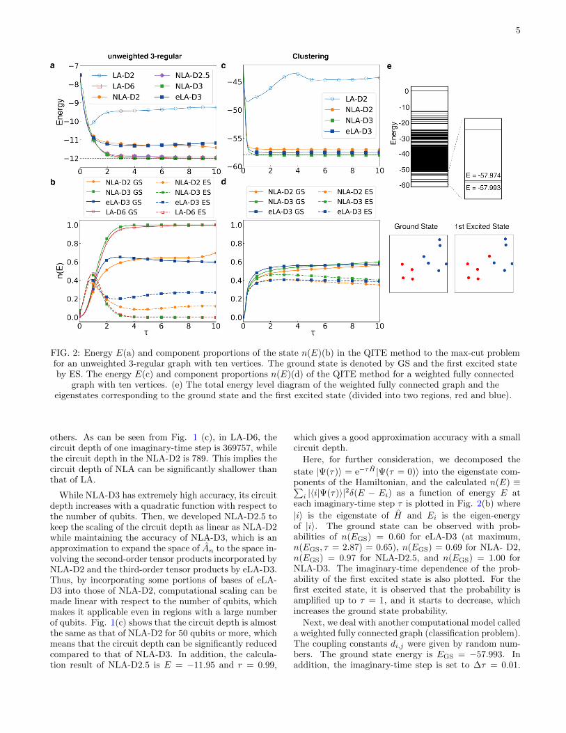
is the energy of the ground state, and it is obtained fromthe exact diagonalization. The energy of the ground stateis EGS = −12. It is known that designing a classicalalgorithm that achieves r > 331/332 for an unweighted3-regular graph is an NP-hard problem [34]. Further, theapproximation accuracy of the current classical algorithmis r ≈ 0.9326 [35]. Figure 2 (a) shows the imaginary-timedependence of the energy. The imaginary-time step wasset to ∆τ = 0.01. In LA-D2, as the imaginary-time τincreased, the energy decreased exponentially in the be-ginning and converged to around−9, which is higher thanthe exact solution by about 3. Another important pointis that the energy does not monotonically decreases alongthe imaginary-time evolution. This behavior indicatesthat the conversion of the operator of the imaginary-time evolution to the unitary operators is less accuratein expanding it in the space of LA-D2. Furthermore,the LA-D6 calculation result shows E = −11.99, whichis the energy almost equal to the exact solution. Wefound that an approximation accuracy in the eLA-D3 isE = −11.17 (r = 0.93) (the lowest value is E = −11.33(r = 0.94)); in NLA-D2, E = −11.42 (r = 0.95); and inNLA-D3, E = −12.00 (r = 1.00). We found that eLA-D3 had an approximation accuracy similar to that of theclassical algorithm, and NLA-D2 had already exceededthe approximation accuracy of the classical algorithm.Note that eLA and NLA monotonically decrease the en-ergy along the imaginary-time evolution with sufficientlygood accuracy compared to LA-D2. This behavior wasconfirmed not only for NLA-D2 but also for NLA-D3 and

5

FIG. 2: Energy E(a) and component proportions of the state n(E)(b) in the QITE method to the max-cut problemfor an unweighted 3-regular graph with ten vertices. The ground state is denoted by GS and the first excited stateby ES. The energy E(c) and component proportions n(E)(d) of the QITE method for a weighted fully connected

graph with ten vertices. (e) The total energy level diagram of the weighted fully connected graph and theeigenstates corresponding to the ground state and the first excited state (divided into two regions, red and blue).

others. As can be seen from Fig. 1 (c), in LA-D6, thecircuit depth of one imaginary-time step is 369757, whilethe circuit depth in the NLA-D2 is 789. This implies thecircuit depth of NLA can be significantly shallower thanthat of LA.

While NLA-D3 has extremely high accuracy, its circuitdepth increases with a quadratic function with respect tothe number of qubits. Then, we developed NLA-D2.5 tokeep the scaling of the circuit depth as linear as NLA-D2while maintaining the accuracy of NLA-D3, which is anapproximation to expand the space of An to the space in-volving the second-order tensor products incorporated byNLA-D2 and the third-order tensor products by eLA-D3.Thus, by incorporating some portions of bases of eLA-D3 into those of NLA-D2, computational scaling can bemade linear with respect to the number of qubits, whichmakes it applicable even in regions with a large numberof qubits. Fig. 1(c) shows that the circuit depth is almostthe same as that of NLA-D2 for 50 qubits or more, whichmeans that the circuit depth can be significantly reducedcompared to that of NLA-D3. In addition, the calcula-tion result of NLA-D2.5 is E = −11.95 and r = 0.99,

which gives a good approximation accuracy with a smallcircuit depth.

Here, for further consideration, we decomposed the

state |Ψ(τ)〉 = e−τH |Ψ(τ = 0)〉 into the eigenstate com-ponents of the Hamiltonian, and the calculated n(E) ≡∑i |〈i|Ψ(τ)〉|2δ(E − Ei) as a function of energy E at

each imaginary-time step τ is plotted in Fig. 2(b) where

|i〉 is the eigenstate of H and Ei is the eigen-energyof |i〉. The ground state can be observed with prob-abilities of n(EGS) = 0.60 for eLA-D3 (at maximum,n(EGS, τ = 2.87) = 0.65), n(EGS) = 0.69 for NLA- D2,n(EGS) = 0.97 for NLA-D2.5, and n(EGS) = 1.00 forNLA-D3. The imaginary-time dependence of the prob-ability of the first excited state is also plotted. For thefirst excited state, it is observed that the probability isamplified up to τ = 1, and it starts to decrease, whichincreases the ground state probability.

Next, we deal with another computational model calleda weighted fully connected graph (classification problem).The coupling constants di,j were given by random num-bers. The ground state energy is EGS = −57.993. Inaddition, the imaginary-time step is set to ∆τ = 0.01.

6

In the classification problem, as shown in Fig. 2(e), eachgraph vertex is colored red or blue. In LA-D2, as inthe 3-regular graph, we observed that the energy doesnot necessarily decrease monotonically. The energy ofeLA-D3 is lower than that of NLA-D2; E = −57.504(r = 0.99) for eLA-D3, E = −57.026(r = 0.98) for NLA-D2, and E = −57.985(r = 0.99) for NLA-D3 (Figure 2(c)). From the viewpoint of the component analyses ofthe states, the ground state and the first excited stateare pseudo-degenerate (Fig. 2.(e)), and therefore, theprobability of the first excited state remains at the samelevel as the ground state even around τ = 2 when the en-ergy converges sufficiently (Fig. 2.(d)). In NLA, the firstexcited state gradually decays along with the imaginary-time evolution; however, a sufficiently long imaginary-time evolution is necessary. In particular, NLA-D2 be-haves similarly to NLA-D3, and NLA-D2 is sufficientlyaccurate to obtain the ground state in actual applica-tions.

Compression of imaginary-time steps

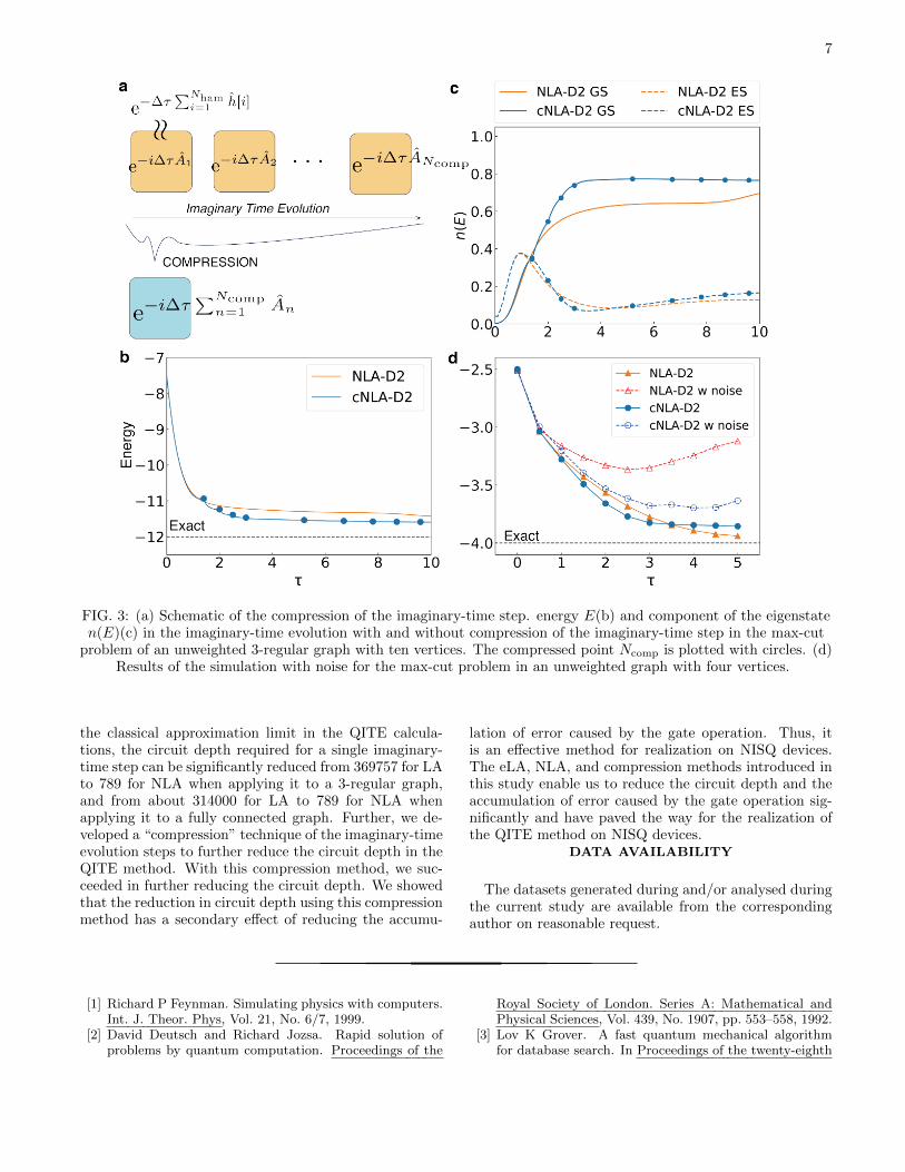
The approximation accuracy of the NLA and its cir-cuit depth have been discussed. The “compression ofimaginary-time steps” is introduced in this section forfurther reduction of the number of gate operations inNLA. Figure 3 (a) shows a schematic of the compres-sion technique. When the imaginary-time step ∆τ issufficiently small, the time-evolution operators can becompressed into a single exponential form via the reverseSuzuki–Trotter decomposition

Ncomp∏n=1

exp(−i∆τAn

)= exp

−i∆τ Ncomp∑n=1

An

+O(∆τ2),

where Ncomp is the number of compressed steps. It isnecessary to choose an appropriate Ncomp within therange that guarantees sufficient accuracy for the Suzuki–Trotter decomposition because its accuracy decreases ifthe Ncomp becomes large. To determine the specificNcomp in this work, we increased the Ncomp parameterby one at every time-evolution step until the total en-ergy increases. In actual QITE calculations, Ncomp is notnecessarily a constant throughout the calculation. Thismethod enables the reduction of quantum circuits to beas small as 1/Ncomp.

The graph used for the calculation is the same as thatin Figures 2(a) and (b), which is a 3-regular graph withten vertices. Figure 3 shows the results of the com-pression technique for the QITE. In Figure 3(b), thetime the compression ended is plotted as a blue cir-cle. In the case of Fig. 3(b), the quantum circuitdepth is significantly reduced by the compression tech-nique to four compressed imaginary-time steps, and theenergy at τ = 10 is E = −11.43 (r = 0.95) withoutand E = −11.59 (r = 0.97) with the compression tech-nique. We found that sufficient accuracy was achieved

regardless of the compression, which indicates compres-sion does not affect the results. It may be assumed thatthe compressed technique has a lower energy than thatof the uncompressed calculation; a detailed investigationrevealed that this was attributed to the accidental accel-eration of the convergence by compression. Figure 3 (c)plots the component analyses of the wavefunctions duringthe imaginary-time evolution with and without the com-pression method. Finally, the probability of obtaining aground state is n(Emin) = 0.76 with and n(Emin) = 0.73without the compression technique.

The “compression of imaginary-time steps” is effectivein reducing the circuit depth, and simultaneously, it re-duces the noise associated with the gate operations. Wediscuss the results of the simulation with noise. The ac-tual qubits are currently connected only with neighboringsites; however, in this study, we simulated a fully con-nected model. For implementation on an actual quan-tum computer, in which only adjacent sites are con-nected, a SWAP gate can be used with an overhead ofO(√Nbit)[36]. For example, QAOA uses a SWAP net-

work [37, 38] to implement a O(Nbit) overhead [39]. Theerror model of the gate was constructed from the ther-mal relaxation time (T1, T2) = (100µs, 80µs), and thegate time (Tg1, Tg2) = (0.02ns, 0.1ns). The noise simu-lation was performed by introducing the readout errors(p00, p01, p10, p11) = (0.995, 0.005, 0.02, 0.98). These pa-rameters were assumed to be close to the actual valuesof IBMQ[40]. Figure 3 (d) shows the simulation resultsof the max-cut problem for an unweighted graph with

four vertices. The coefficients a(n){i,l} in Eq. (3) for the

noisy calculation are the same as those for the non-noisycalculation. The noiseless condition without compressionresults in E = −3.94, which is close to the exact solutionE = −4.00 around τ = 5. However, the circuit depth is922 (∆τ = 0.5), and the simulation result with noise isE = −3.13, which is far from the exact solution. Thisgap was attributed to the accumulation of errors causedby an increase in circuit depth. The result with compres-sion is E = −3.85 in the case without noise; however, thecircuit depth is 163, and the effect of noise is expectedto be less sensitive. In fact, the simulation result withnoise is E = −3.63, which shows that the noise can bereduced with compression. Thus, it has been shown thatthe “compression” method of quantum circuits has anadvantage of reducing the accumulation of errors.

CONCLUDING REMARKS

In this study, we proposed two-step approximationmethods based on nonlocality: eLA and NLA. We ap-plied them to the Max-cut problem of an unweighted 3-regular graph and a weighted fully-connected graph, andcomparatively validated the performances of LA, eLA,and NLA. We found that NLA requires significantly lesscircuit depth than LA while maintaining the same level ofcomputational accuracy. For example, when we request

7

FIG. 3: (a) Schematic of the compression of the imaginary-time step. energy E(b) and component of the eigenstaten(E)(c) in the imaginary-time evolution with and without compression of the imaginary-time step in the max-cut

problem of an unweighted 3-regular graph with ten vertices. The compressed point Ncomp is plotted with circles. (d)Results of the simulation with noise for the max-cut problem in an unweighted graph with four vertices.

the classical approximation limit in the QITE calcula-tions, the circuit depth required for a single imaginary-time step can be significantly reduced from 369757 for LAto 789 for NLA when applying it to a 3-regular graph,and from about 314000 for LA to 789 for NLA whenapplying it to a fully connected graph. Further, we de-veloped a “compression” technique of the imaginary-timeevolution steps to further reduce the circuit depth in theQITE method. With this compression method, we suc-ceeded in further reducing the circuit depth. We showedthat the reduction in circuit depth using this compressionmethod has a secondary effect of reducing the accumu-

lation of error caused by the gate operation. Thus, itis an effective method for realization on NISQ devices.The eLA, NLA, and compression methods introduced inthis study enable us to reduce the circuit depth and theaccumulation of error caused by the gate operation sig-nificantly and have paved the way for the realization ofthe QITE method on NISQ devices.

DATA AVAILABILITY

The datasets generated during and/or analysed duringthe current study are available from the correspondingauthor on reasonable request.

[1] Richard P Feynman. Simulating physics with computers.Int. J. Theor. Phys, Vol. 21, No. 6/7, 1999.

[2] David Deutsch and Richard Jozsa. Rapid solution ofproblems by quantum computation. Proceedings of the

Royal Society of London. Series A: Mathematical andPhysical Sciences, Vol. 439, No. 1907, pp. 553–558, 1992.

[3] Lov K Grover. A fast quantum mechanical algorithmfor database search. In Proceedings of the twenty-eighth

8

annual ACM symposium on Theory of computing, pp.212–219, 1996.

[4] Peter W Shor. Polynomial-time algorithms for prime fac-torization and discrete logarithms on a quantum com-puter. SIAM review, Vol. 41, No. 2, pp. 303–332, 1999.

[5] Frank Arute, Kunal Arya, Ryan Babbush, Dave Bacon,Joseph C Bardin, Rami Barends, Rupak Biswas, SergioBoixo, Fernando GSL Brandao, David A Buell, et al.Quantum supremacy using a programmable supercon-ducting processor. Nature, Vol. 574, No. 7779, pp. 505–510, 2019.

[6] Laurent Hyafil and Ronald L Rivest. Graph partitioningand constructing optimal decision trees are polynomialcomplete problems. IRIA. Laboratoire de Recherche enInformatique et Automatique, 1973.

[7] Eugene L Lawler. The traveling salesman prob-lem: a guided tour of combinatorial optimization.Wiley-Interscience Series in Discrete Mathematics, 1985.

[8] Nhu Binh Ho and Joc Cing Tay. Genace: an efficientcultural algorithm for solving the flexible job-shop prob-lem. In Proceedings of the 2004 Congress on EvolutionaryComputation (IEEE Cat. No. 04TH8753), Vol. 2, pp.1759–1766. IEEE, 2004.

[9] Richard M Karp. Reducibility among combinatorialproblems. In Complexity of computer computations, pp.85–103. Springer, 1972.

[10] Christoph Durr and Peter Hoyer. A quantum al-gorithm for finding the minimum. arXiv preprintquant-ph/9607014, 1996.

[11] William P Baritompa, David W Bulger, and Graham RWood. Grover’s quantum algorithm applied to globaloptimization. SIAM Journal on Optimization, Vol. 15,No. 4, pp. 1170–1184, 2005.

[12] John Preskill. Quantum computing in the nisq era andbeyond. Quantum, Vol. 2, p. 79, 2018.

[13] Alberto Peruzzo, Jarrod McClean, Peter Shadbolt,Man-Hong Yung, Xiao-Qi Zhou, Peter J Love, AlanAspuru-Guzik, Jeremy LO’brien. A variational eigen-value solver on a photonic quantum processor. Naturecommunications, Vol. 5, p. 4213, 2014.

[14] Jarrod R McClean, Jonathan Romero, Ryan Babbush,and Alan Aspuru-Guzik. The theory of variational hybridquantum-classical algorithms. New Journal of Physics,Vol. 18, No. 2, p. 023023, 2016.

[15] Edward Farhi, Jeffrey Goldstone, and Sam Gutmann.A quantum approximate optimization algorithm. arXivpreprint arXiv:1411.4028, 2014.

[16] JS Otterbach, R Manenti, N Alidoust, A Bestwick,M Block, B Bloom, S Caldwell, N Didier, E SchuylerFried, S Hong, et al. Unsupervised machine learn-ing on a hybrid quantum computer. arXiv preprintarXiv:1712.05771, 2017.

[17] Nikolaj Moll, Panagiotis Barkoutsos, Lev S Bishop,Jerry M Chow, Andrew Cross, Daniel J Egger, Stefan Fil-ipp, Andreas Fuhrer, Jay M Gambetta, Marc Ganzhorn,et al. Quantum optimization using variational algorithmson near-term quantum devices. Quantum Science andTechnology, Vol. 3, No. 3, p. 030503, 2018.

[18] Zhihui Wang, Stuart Hadfield, Zhang Jiang, andEleanor G Rieffel. Quantum approximate optimizationalgorithm for maxcut: A fermionic view. Physical ReviewA, Vol. 97, No. 2, p. 022304, 2018.

[19] Stuart Hadfield, Zhihui Wang, Bryan O’Gorman,Eleanor G. Rieffel, Davide Venturelli, and Rupak Biswas.

From the quantum approximate optimization algorithmto a quantum alternating operator ansatz. Algorithms,Vol. 12, p. 34, 2019.

[20] Gian Giacomo Guerreschi and Anne Y Matsuura. Qaoafor max-cut requires hundreds of qubits for quantumspeed-up. Scientific reports, Vol. 9, , 2019.

[21] Jarrod R McClean, Sergio Boixo, Vadim N Smelyanskiy,Ryan Babbush, and Hartmut Neven. Barren plateausin quantum neural network training landscapes. Naturecommunications, Vol. 9, No. 1, pp. 1–6, 2018.

[22] Andrew Lucas. Ising formulations of many np problems.ArXiv, Vol. abs/1302.5843, , 2014.

[23] Sam McArdle, Tyson Jones, Suguru Endo, Ying Li, Si-mon C Benjamin, and Xiao Yuan. Variational ansatz-based quantum simulation of imaginary time evolution.npj Quantum Information, Vol. 5, No. 1, pp. 1–6, 2019.

[24] James Stokes, Josh Izaac, Nathan Killoran, and GiuseppeCarleo. Quantum natural gradient. arXiv preprintarXiv:1909.02108, 2019.

[25] Wierichs David, Gogolin Christian, and KastoryanoMichael. Avoiding local minima in variational quantumeigensolvers with the natural gradient optimizert. arXivpreprint arXiv:2004.14666, 2020.

[26] Mario Motta, Chong Sun, Adrian TK Tan,Matthew JO’Rourke, Erika Ye, Austin J Minnich,Fernando GSL Brandao, Garnet Kin-Lic Chan. Deter-mining eigenstates and thermal states on a quantumcomputer using quantum imaginary time evolution.Nature Physics, Vol. 16, No. 2, pp. 205–210, 2020.

[27] Kubra Yeter-Aydeniz, Raphael C Pooser, and GeorgeSiopsis. Practical quantum computation of chemicaland nuclear energy levels using quantum imaginarytime evolution and lanczos algorithms. arXiv preprintarXiv:1912.06226, 2019.

[28] Matthew JS Beach, Roger G Melko, Tarun Grover, andTimothy H Hsieh. Making trotters sprint: A variationalimaginary time ansatz for quantum many-body systems.Physical Review B, Vol. 100, No. 9, p. 094434, 2019.

[29] Anil K Jain, M Narasimha Murty, and Patrick J Flynn.Data clustering: a review. ACM computing surveys(CSUR), Vol. 31, No. 3, pp. 264–323, 1999.

[30] Anil K Jain and Richard C Dubes. Algorithms forclustering data. Prentice-Hall, Inc., 1988.

[31] Sergey B. Bravyi and Alexei Yu. Kitaev. Fermionic quan-tum computation. Annals of Physics, Vol. 298, No. 1, pp.210–226, 2002.

[32] P. Jordan and E. P. Wigner. Uber das paulische

Aquivalenzverbot. European Physical Journal, Vol. 47,No. 9, pp. 631–651, 1928.

[33] Gadi Aleksandrowicz, Thomas Alexander, PanagiotisBarkoutsos, Luciano Bello, Yael Ben-Haim, D Bucher,FJ Cabrera-Hernandez, J Carballo-Franquis, A Chen,CF Chen, et al. Qiskit: An open-source framework forquantum computing. Accessed on: Mar, Vol. 16, , 2019.

[34] Piotr Berman and Marek Karpinski. On some tighterinapproximability results (extended abstract). In ICAL’99 Proceedings of the 26th International Colloquium onAutomata, Languages and Programming, pp. 200–209,1999.

[35] Michel X. Goemans and David P. Williamson. Improvedapproximation algorithms for maximum cut and satisfia-bility problems using semidefinite programming. Journalof the ACM, Vol. 42, No. 6, pp. 1115–1145, 1995.

9

[36] Donny Cheung, Dmitri Maslov, and Simone Severini.Translation techniques between quantum circuit architec-tures. In Workshop on Quantum Information Processing,2007.

[37] Ian D Kivlichan, Jarrod McClean, Nathan Wiebe, CraigGidney, Alan Aspuru-Guzik, Garnet Kin-Lic Chan, andRyan Babbush. Quantum simulation of electronic struc-ture with linear depth and connectivity. Physical reviewletters, Vol. 120, No. 11, p. 110501, 2018.

[38] Ryan Babbush, Nathan Wiebe, Jarrod McClean, JamesMcClain, Hartmut Neven, and Garnet Kin-Lic Chan.Low-depth quantum simulation of materials. PhysicalReview X, Vol. 8, No. 1, p. 011044, 2018.

[39] Gavin E. Crooks. Performance of the quantum approxi-mate optimization algorithm on the maximum cut prob-lem. arXiv preprint arXiv:1811.08419, 2018.

[40] IBM Quantum Experience Web Site. .https://

quantum-computing.ibm.com/.

ACKNOWLEDGEMENT

This research was supported by MEXT as an Ex-ploratory Challenge on Post-K computer (Frontiers ofBasic Science: Challenging the Limits) and by Grants-in-Aid for Scientific Research (A) (Grant Numbers18H03770) from JSPS (Japan Society for the Promotionof Science).

AUTHOR CONTRIBUTIONS

H. N. and Y. M. conceived the general idea. H. N.modified the code provided in prior work. H.N. and T. K.developed the code for noisy simulation. Numerical sim-ulations were performed by H.N. All authors contributedequally to the manuscript preparation and presentationof results.