Nonparametric Estimation Nonparametric Estimation with Recurrent Event Datawith Recurrent Event Data

Edsel A. Pena

Department of Statistics

University of South Carolina

E-mail: pena@stat.sc.edu

Research supported by NIH and NSF Grants

Based on joint works with R. Strawderman (Cornell) and M. Hollander (Florida State)

Talk at UNCC, 10/12/01

2

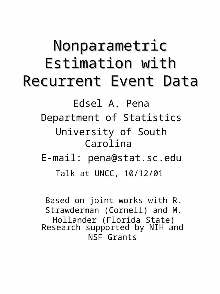
A Real Recurrent Event Data(Source: Aalen and Husebye (‘91), Statistics

in Medicine)

Unit #i

#Complete(Ki=K(i))

Complete Observed SuccessivePeriods (Tij)

Censored(i - SiK(i))

1 8 112 145 39 52 21 34 33 51 542 2 206 147 303 3 284 59 186 44 3 94 98 84 875 1 67 1316 9 124 34 87 75 43 38 58 142 75 237 5 116 71 83 68 125 1118 4 111 59 47 95 1109 4 98 161 154 55 4410 2 166 56 12211 5 63 90 63 103 51 8512 4 47 86 68 144 7213 3 120 106 176 614 4 112 25 57 166 8515 3 132 267 89 8616 5 120 47 165 64 113 1217 4 162 141 107 69 3918 6 106 56 158 41 41 168 1319 5 147 134 78 66 100 4

Variable: Migrating motor complex (MMC) periods, in minutes, for 19 individuals in a study concerning small bowel motility during fasting state.

3

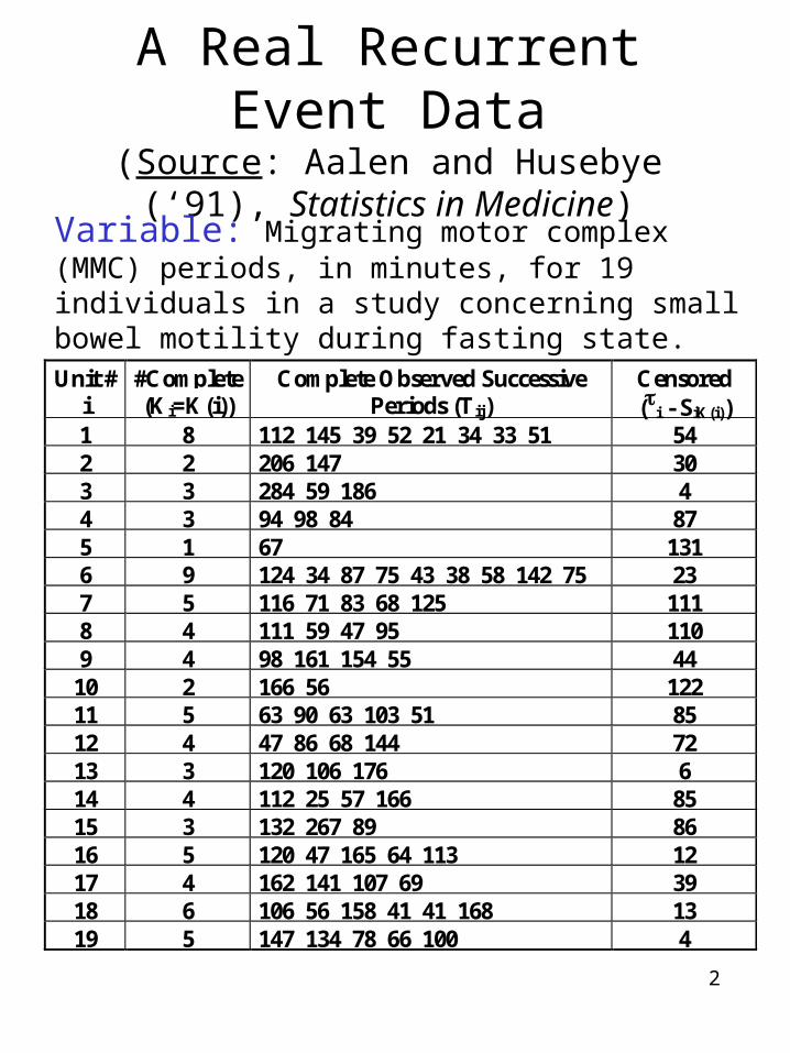
Pictorial Representation of Data for a Unit or Subject

• Consider unit/subject #3.

• K = 3

• Gap Times, Tj: 284, 343, 529

• Censored Time, -SK: 4

• Calendar Times, Sj: 284, 343, 529

• Limit of Obs. Period:

=533S1=284 S2=343 S3=5290

T1 T2 T3

T4

Calendar Scale

4

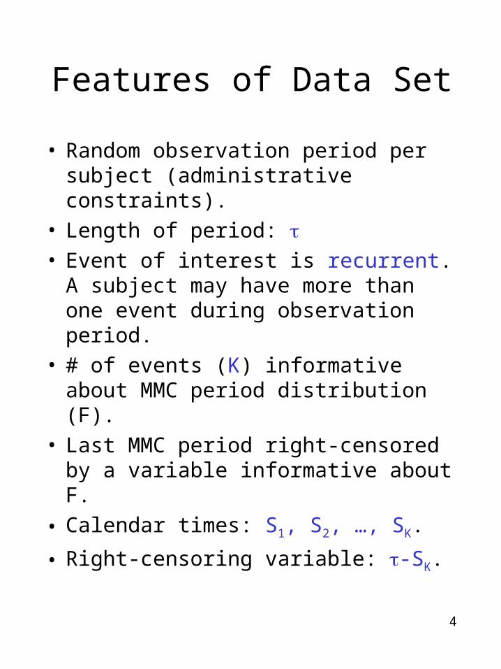
Features of Data Set

• Random observation period per subject (administrative constraints).

• Length of period: • Event of interest is recurrent. A

subject may have more than one event during observation period.

• # of events (K) informative about MMC period distribution (F).

• Last MMC period right-censored by a variable informative about F.

• Calendar times: S1, S2, …, SK.

• Right-censoring variable: -SK.

5

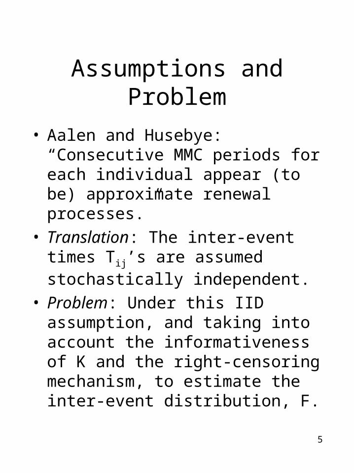
Assumptions and Problem

• Aalen and Husebye: “Consecutive MMC periods for each individual appear (to be) approximate renewal processes.”

• Translation: The inter-event times Tij’s are assumed stochastically independent.

• Problem: Under this IID assumption, and taking into account the informativeness of K and the right-censoring mechanism, to estimate the inter-event distribution, F.

6

General Form of Data Accrual

Unit#

Successive Inter-EventTimes or Gaptimes

Length ofStudy Period

1 T11, T12, …, T1j, … IID F 1

2 T21, T22, …, T2j, … IID F 2

… … …n Tn1, Tn2, …, Tnj, … IID F

n

Calendar Times of Event Occurrences

Si0=0 and Sij = Ti1 + Ti2 + … + Tij

Number of Events in Observation Period

Ki = max{j: Sij < i}

Upper limit of observation periods, ’s, could be fixed, or assumed to be IID with unknown distribution G.

7

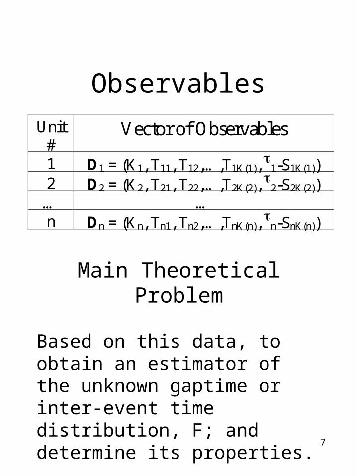
Observables

Unit#

Vector of Observables

1 D1 = (K1, T11, T12,…,T1K(1), 1-S1K(1))2 D2 = (K2, T21, T22,…,T2K(2), 2-S2K(2))… …n Dn = (Kn, Tn1, Tn2,…,TnK(n), n-SnK(n))

Main Theoretical Problem

Based on this data, to obtain an estimator of the unknown gaptime or inter-event time distribution, F; and determine its properties.

8

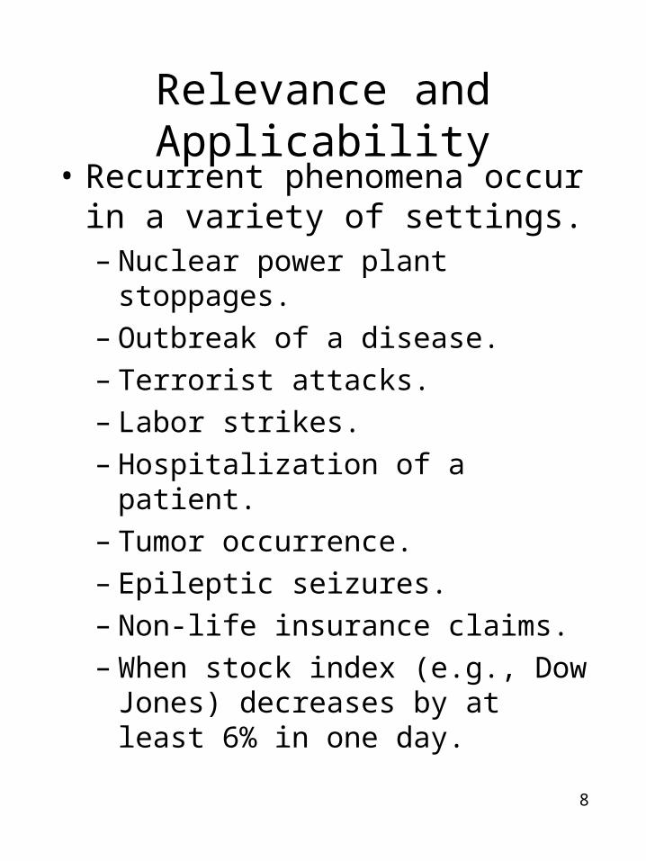
Relevance and Applicability

• Recurrent phenomena occur in a variety of settings.– Nuclear power plant stoppages.– Outbreak of a disease.– Terrorist attacks.– Labor strikes.– Hospitalization of a patient.– Tumor occurrence.– Epileptic seizures.– Non-life insurance claims.– When stock index (e.g., Dow

Jones) decreases by at least 6% in one day.

9

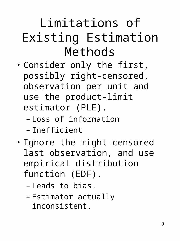
Limitations of Existing Estimation Methods

• Consider only the first, possibly right-censored, observation per unit and use the product-limit estimator (PLE). – Loss of information– Inefficient

• Ignore the right-censored last observation, and use empirical distribution function (EDF).– Leads to bias.– Estimator actually inconsistent.

10

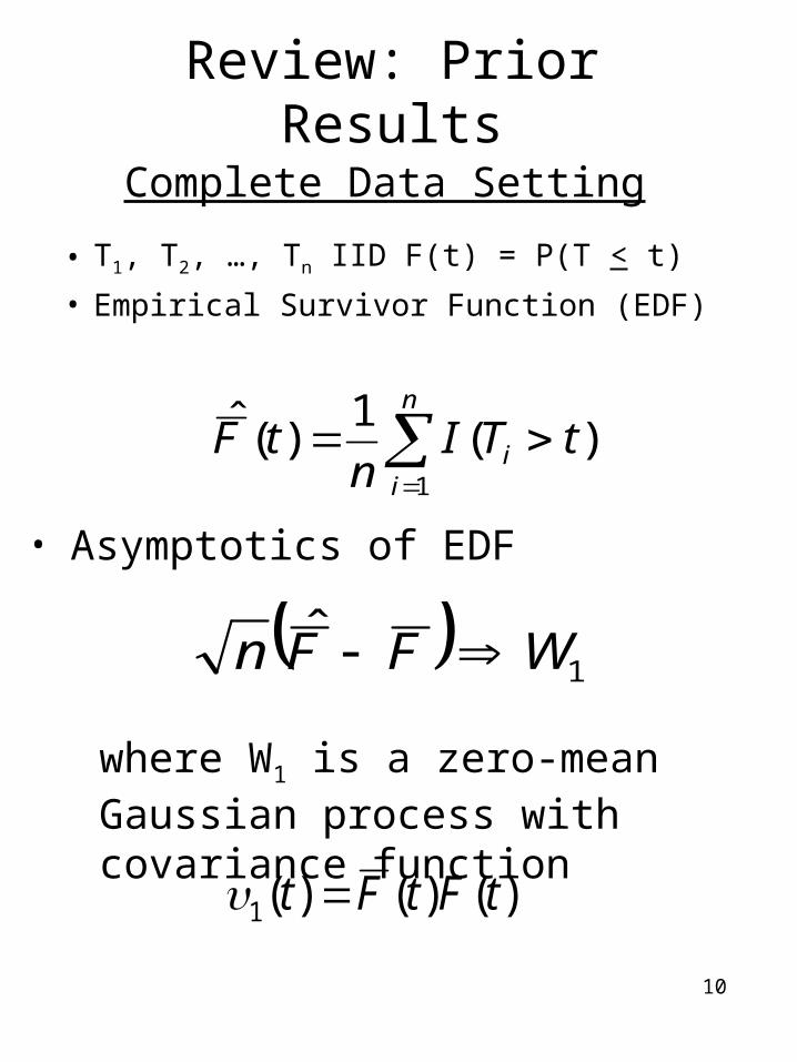
Review: Prior Results

• T1, T2, …, Tn IID F(t) = P(T < t)

• Empirical Survivor Function (EDF)

)(1

)(ˆ

1

tTIn

tFn

ii

• Asymptotics of EDF

1ˆ WFFn

where W1 is a zero-mean Gaussian process with covariance function

).()()(1 tFtFt

Complete Data Setting

11

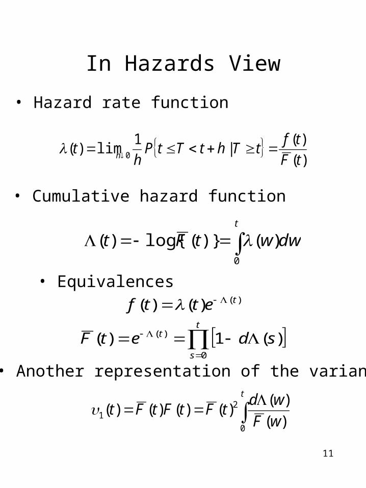
In Hazards View

• Hazard rate function

)(

)(|

1lim)(

0 tF

tftThtTtP

ht

h

• Cumulative hazard function

t

dwwtFt0

)()}(log{)(

• Equivalences

t

s

t

t

sdetF

ettf

0

)(

)(

)(1)(

)()(

• Another representation of the variance

t

wF

wdtFtFtFt

0

21 )(

)()()()()(

12

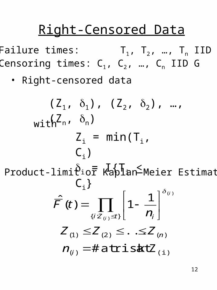
Right-Censored Data

• Failure times: T1, T2, …, Tn IID F• Censoring times: C1, C2, …, Cn IID G

• Right-censored data

(Z1, 1), (Z2, 2), …, (Zn, n)

Zi = min(Ti, Ci)i = I{Ti < Ci}

with

• Product-limit or Kaplan-Meier Estimator

(i))(

)()2()1(

}:{

Zat risk at #

...

11)(ˆ

)(

)(

i

n

tZi i

n

ZZZ

ntF

i

i

13

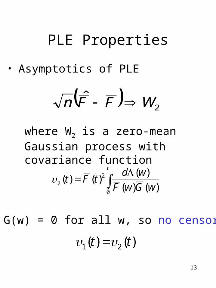
PLE Properties

• Asymptotics of PLE

2ˆ WFFn

where W2 is a zero-mean Gaussian process with covariance function

t

wGwF

wdtFt

0

22 )()(

)()()(

• If G(w) = 0 for all w, so no censoring,

)()( 21 tt

14

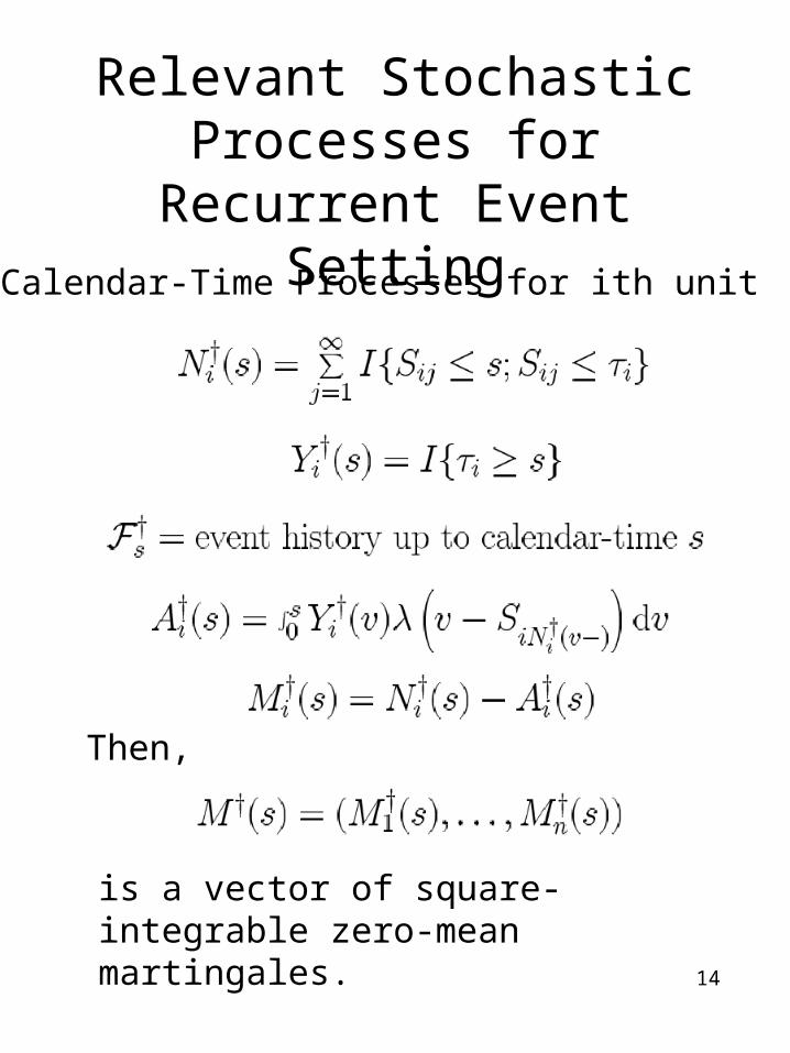
Relevant Stochastic Processes for Recurrent Event Setting

• Calendar-Time Processes for ith unit

is a vector of square-integrable zero-mean martingales.

Then,

15

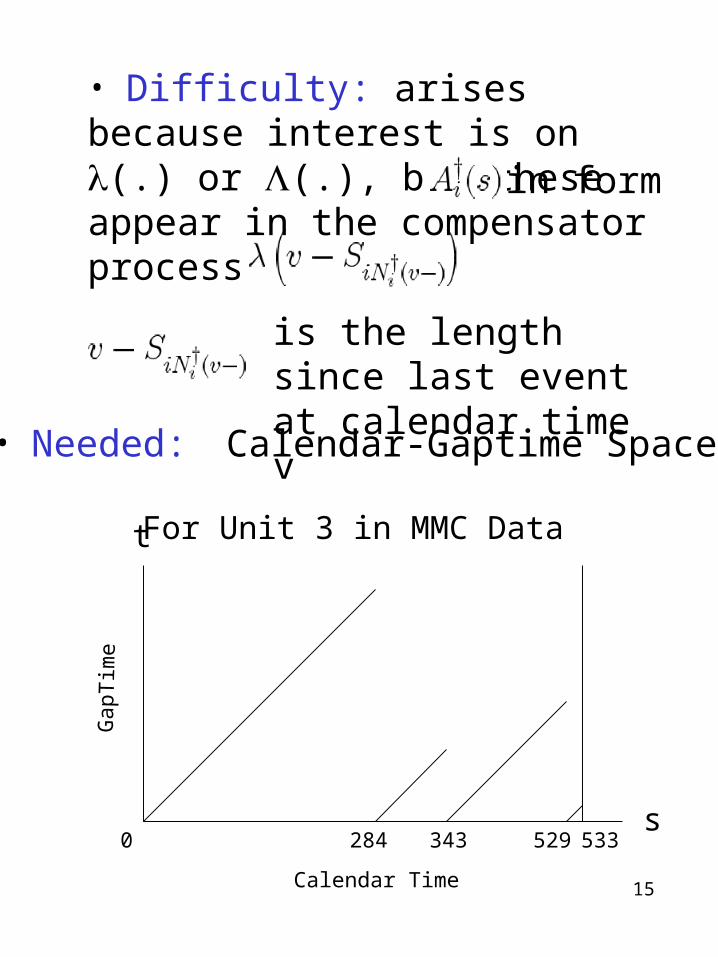
is the length since last event at calendar time v

• Needed: Calendar-Gaptime Space

0

• Difficulty: arises because interest is on (.) or (.), but these appear in the compensator process in form

Gap

Tim

e

Calendar Time

533284 343 529s

t For Unit 3 in MMC Data

16

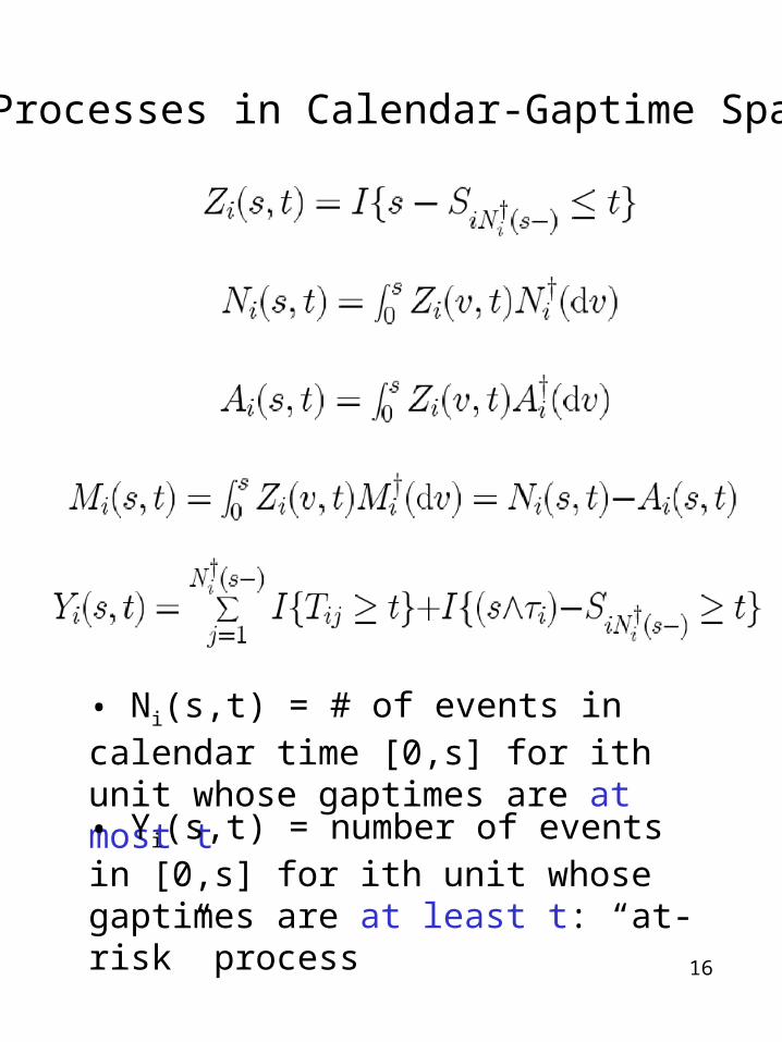
• Processes in Calendar-Gaptime Space

• Ni(s,t) = # of events in calendar time [0,s] for ith unit whose gaptimes are at most t

• Yi(s,t) = number of events in [0,s] for ith unit whose gaptimes are at least t: “at-risk” process

17

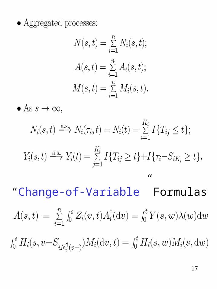
“Change-of-Variable” Formulas

18

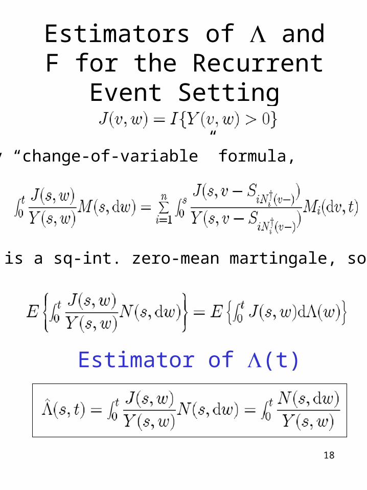
Estimators of and F for the Recurrent Event Setting

By “change-of-variable” formula,

RHS is a sq-int. zero-mean martingale, so

Estimator of (t)

19

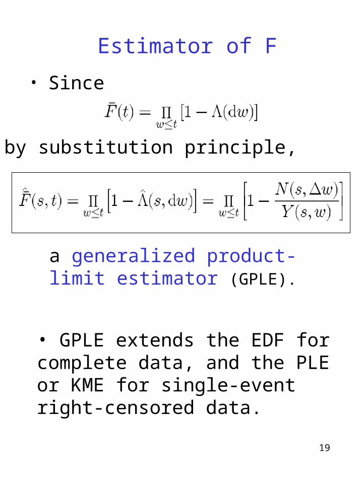
Estimator of F

• Since

by substitution principle,

a generalized product-limit estimator (GPLE).

• GPLE extends the EDF for complete data, and the PLE or KME for single-event right-censored data.

20

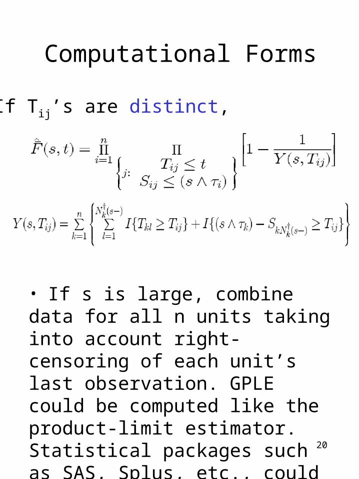
Computational Forms

• If Tij’s are distinct,

• If s is large, combine data for all n units taking into account right-censoring of each unit’s last observation. GPLE could be computed like the product-limit estimator. Statistical packages such as SAS, Splus, etc., could be utilized.

21

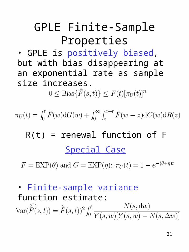
GPLE Finite-Sample Properties

• GPLE is positively biased, but with bias disappearing at an exponential rate as sample size increases.

• Finite-sample variance function estimate:

Special Case

R(t) = renewal function of F

22

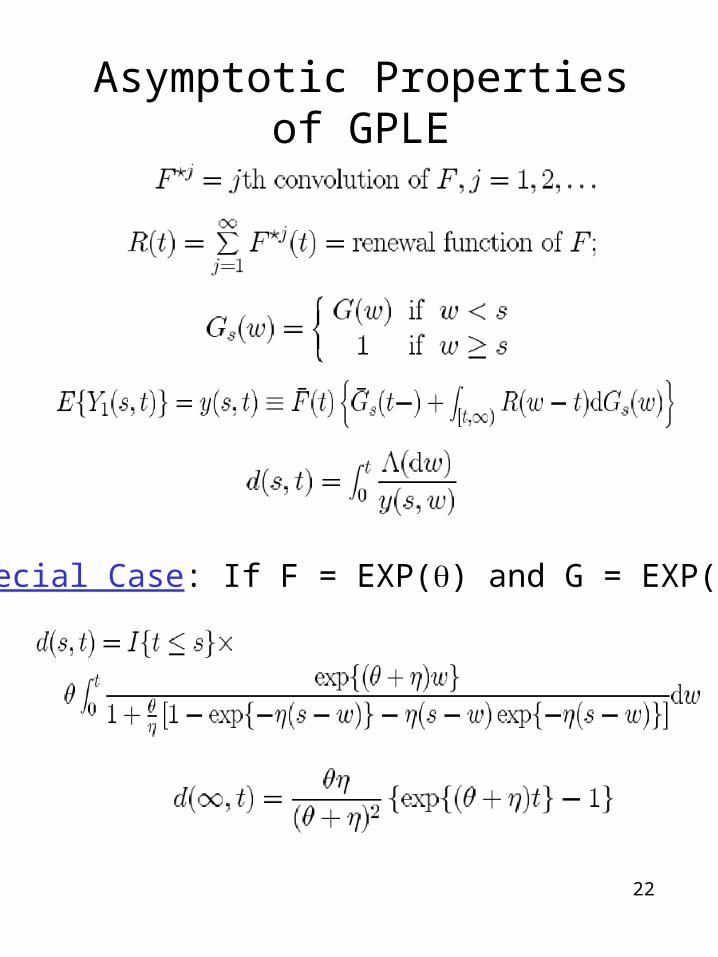
Asymptotic Properties of GPLE

Special Case: If F = EXP() and G = EXP()

23

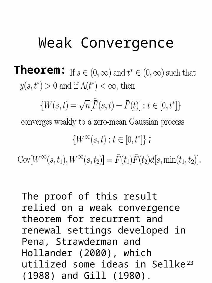
Weak Convergence

Theorem:

;

The proof of this result relied on a weak convergence theorem for recurrent and renewal settings developed in Pena, Strawderman and Hollander (2000), which utilized some ideas in Sellke (1988) and Gill (1980).

24

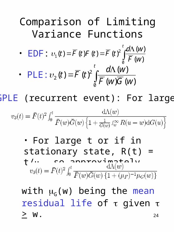
Comparison of Limiting Variance Functions

• PLE:

t

wGwF

wdtFt

0

22 )()(

)()()(

• GPLE (recurrent event): For large s,

• For large t or if in stationary state, R(t) = t/F, so approximately,

with G(w) being the mean residual life of given > w.

• EDF:

t

wF

wdtFtFtFt

0

21 )(

)()()()()(

25

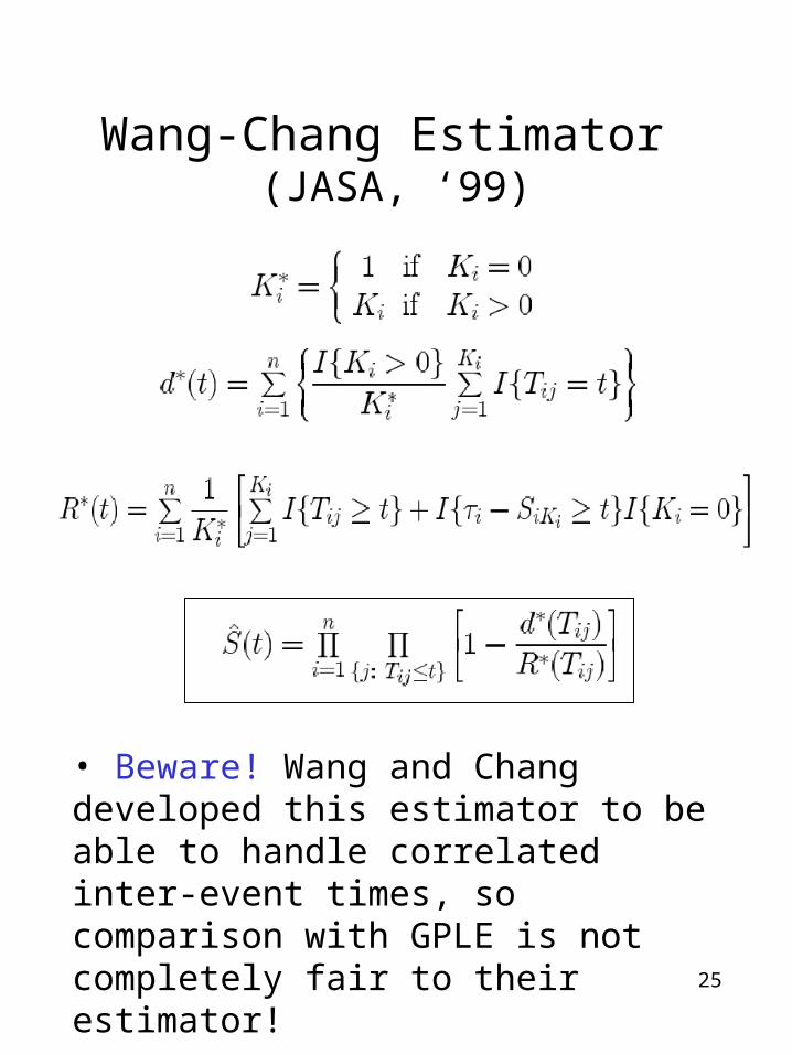
Wang-Chang Estimator (JASA, ‘99)

• Beware! Wang and Chang developed this estimator to be able to handle correlated inter-event times, so comparison with GPLE is not completely fair to their estimator!

26

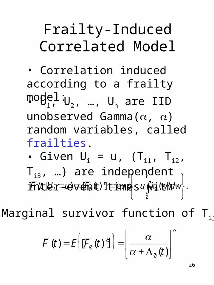
Frailty-Induced Correlated Model

• Correlation induced according to a frailty model:

• U1, U2, …, Un are IID unobserved Gamma(, ) random variables, called frailties.• Given Ui = u, (Ti1, Ti2, Ti3, …) are independent inter-event times with

.)(exp)]([)|(0

00

tu

i dwwutFuUtF

• Marginal survivor function of Tij:

)(

)]([)(0

0 ttFEtF U

27

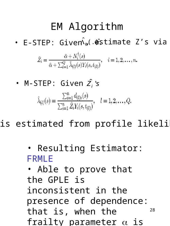
Frailty-Model Estimator

• Frailty parameter, , determines dependence among inter-event times.

• Small (Large) : Strong (Weak) dependence.

• EM algorithm is needed to obtain the estimator, where the unobserved frailties are viewed as missing values.

• EM implementation parallels that of Nielsen, Gill, Andersen, and Sorensen (1992).

28

• Resulting Estimator: FRMLE• Able to prove that the GPLE is inconsistent in the presence of dependence: that is, when the frailty parameter is finite.

• E-STEP: Given ̂(.),ˆ0 , estimate Z’s via

, • M-STEP: Given sZi 'ˆ

is estimated from profile likelihood.

EM Algorithm

29

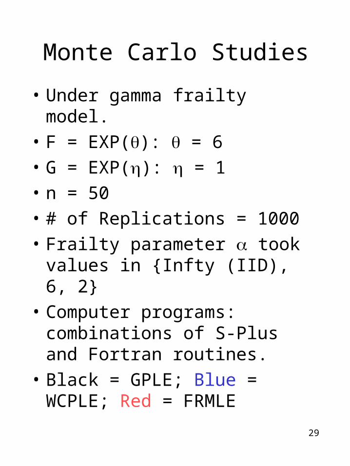
Monte Carlo Studies

• Under gamma frailty model.

• F = EXP(): = 6

• G = EXP(): = 1

• n = 50

• # of Replications = 1000

• Frailty parameter took values in {Infty (IID), 6, 2}

• Computer programs: combinations of S-Plus and Fortran routines.

• Black = GPLE; Blue = WCPLE; Red = FRMLE

30

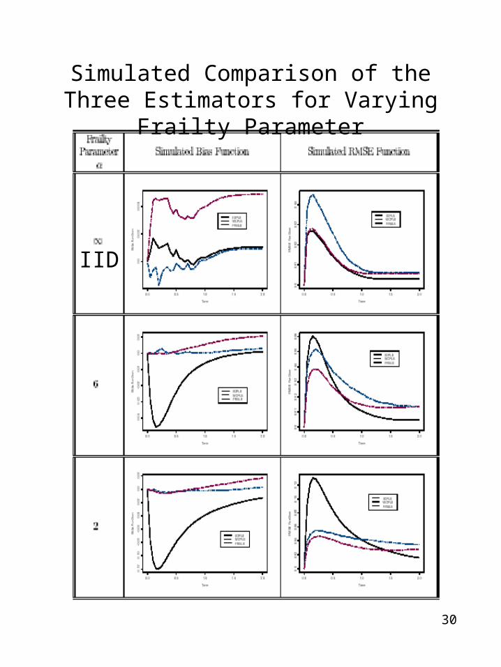
IID

Simulated Comparison of the Three Estimators for Varying Frailty Parameter

31

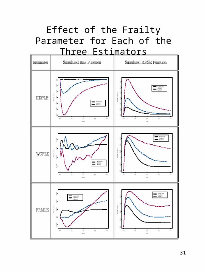
Effect of the Frailty Parameter for Each of the Three Estimators

32

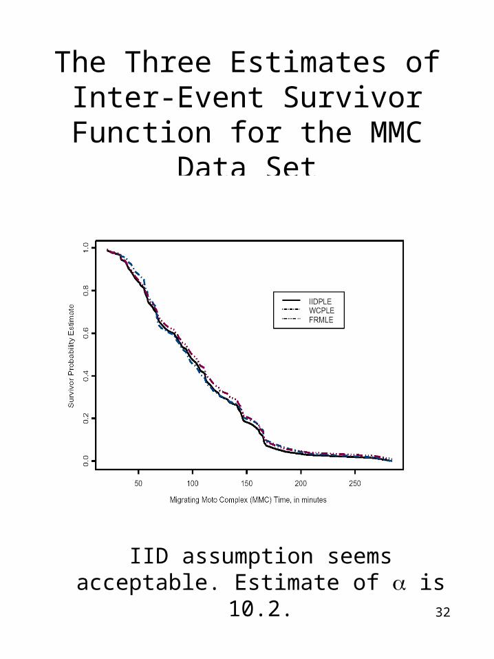
The Three Estimates of Inter-Event Survivor Function for the

MMC Data Set

IID assumption seems acceptable. Estimate of is 10.2.