Embed Size (px)
Citation preview

Minimax optimal alternating minimizationfor kernel nonparametric tensor learning
†‡ Taiji Suzukijoint work with †Heishiro Kanagawa, ⋄Hayato Kobayashi, ⋄Nobuyuki Shimizu
and ⋄Yukihiro Tagami
†Tokyo Institute of TechnologyDepartment of Mathematical Computing Sciences
‡JST, PRESTO and AIP, RIKEN⋄Yahoo! Japan.
19th/Jan/2017PFN主催 NIPS2016読み会
1 / 41
Outline
1 Introduction
2 Basics of low rank tensor decomposition
3 Nonparametric tensor estimationAlternating minimizationConvergence analysisReal data analysis: multitask learning
2 / 41
Outline
1 Introduction
2 Basics of low rank tensor decomposition
3 Nonparametric tensor estimationAlternating minimizationConvergence analysisReal data analysis: multitask learning
3 / 41
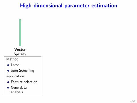
High dimensional parameter estimation
VectorSparsity
MatrixLow rank
TensorLow rank
Method
Lasso
Sure Screening
Application
Feature selection
Gene dataanalysis
Method
PCA
Trace norm reg.
Application
Dim. Reduction
Recommendationsystem
Three layer NN
This studyHigher order relation
4 / 41
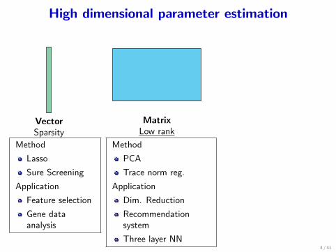
High dimensional parameter estimation
VectorSparsity
MatrixLow rank
TensorLow rank
Method
Lasso
Sure Screening
Application
Feature selection
Gene dataanalysis
Method
PCA
Trace norm reg.
Application
Dim. Reduction
Recommendationsystem
Three layer NN
This studyHigher order relation
4 / 41
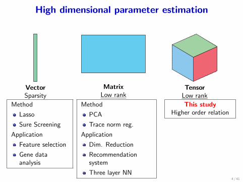
High dimensional parameter estimation
VectorSparsity
MatrixLow rank
TensorLow rank
Method
Lasso
Sure Screening
Application
Feature selection
Gene dataanalysis
Method
PCA
Trace norm reg.
Application
Dim. Reduction
Recommendationsystem
Three layer NN
This studyHigher order relation
4 / 41
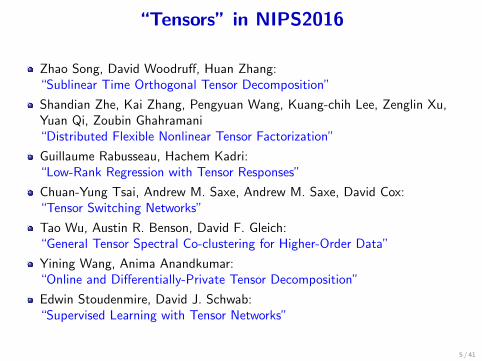
“Tensors” in NIPS2016
Zhao Song, David Woodruff, Huan Zhang:“Sublinear Time Orthogonal Tensor Decomposition”
Shandian Zhe, Kai Zhang, Pengyuan Wang, Kuang-chih Lee, Zenglin Xu,Yuan Qi, Zoubin Ghahramani“Distributed Flexible Nonlinear Tensor Factorization”
Guillaume Rabusseau, Hachem Kadri:“Low-Rank Regression with Tensor Responses”
Chuan-Yung Tsai, Andrew M. Saxe, Andrew M. Saxe, David Cox:“Tensor Switching Networks”
Tao Wu, Austin R. Benson, David F. Gleich:“General Tensor Spectral Co-clustering for Higher-Order Data”
Yining Wang, Anima Anandkumar:“Online and Differentially-Private Tensor Decomposition”
Edwin Stoudenmire, David J. Schwab:“Supervised Learning with Tensor Networks”
5 / 41
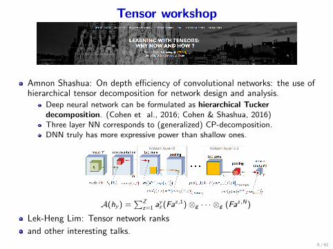
Tensor workshop
Amnon Shashua: On depth efficiency of convolutional networks: the use ofhierarchical tensor decomposition for network design and analysis.
Deep neural network can be formulated as hierarchical Tuckerdecomposition. (Cohen et al., 2016; Cohen & Shashua, 2016)Three layer NN corresponds to (generalized) CP-decomposition.DNN truly has more expressive power than shallow ones.
A(hy ) =∑Z
z=1 ayz (Fa
z,1)⊗g · · · ⊗g (Faz,N)
Lek-Heng Lim: Tensor network ranks
and other interesting talks.
6 / 41
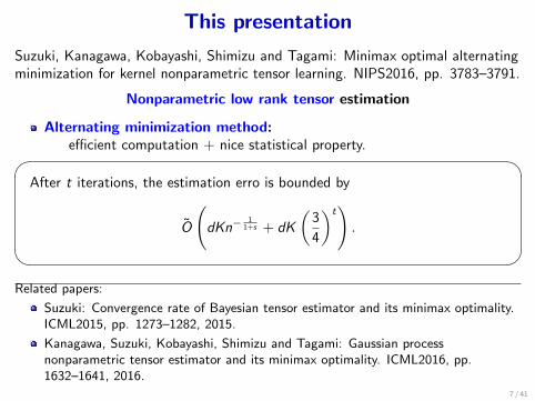
This presentation
Suzuki, Kanagawa, Kobayashi, Shimizu and Tagami: Minimax optimal alternatingminimization for kernel nonparametric tensor learning. NIPS2016, pp. 3783–3791.
Nonparametric low rank tensor estimation
Alternating minimization method:efficient computation + nice statistical property.� �
After t iterations, the estimation erro is bounded by
O
(dKn−
11+s + dK
(3
4
)t).
� �Related papers:
Suzuki: Convergence rate of Bayesian tensor estimator and its minimax optimality.ICML2015, pp. 1273–1282, 2015.
Kanagawa, Suzuki, Kobayashi, Shimizu and Tagami: Gaussian processnonparametric tensor estimator and its minimax optimality. ICML2016, pp.1632–1641, 2016.
7 / 41

Error bound comparisonParametric tensor model (CP-decomposition)
Method Least squares Convex reg. Bayesvia matricization
Error bound
∏Kk=1 Mk
n
dK/2√∏
k Mk
n
d(∑K
k=1 Mk) log(n)
nK : dimension of the tensor, d : rank, Mk : size
Convex reg.: Tomioka et al. (2011); Tomioka and Suzuki (2013); Zheng andTomioka (2015); Mu et al. (2014)
Bayes: Suzuki (2015)
Nonparametric tensor model (CP-decomposition)Method Naive method Bayes/
Alternating min.
Error bound n−1
1+Ks dKn−1
1+s
K : size, s: complexity of the model space
Bayes: Kanagawa et al. (2016)
Alternating minimization: This paper.8 / 41

Outline
1 Introduction
2 Basics of low rank tensor decomposition
3 Nonparametric tensor estimationAlternating minimizationConvergence analysisReal data analysis: multitask learning
9 / 41
Tensor decompositions
CP-decomposition
Tucker decomposition
Tensor train
Tensor network
10 / 41
Tensor rank: CP-rank
=A
B
C+ +…+
a1
b1
c1
a2
b2
c2
ad
bd
cd
=
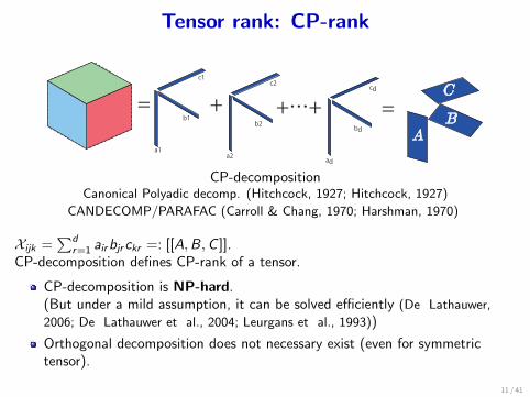
CP-decompositionCanonical Polyadic decomp. (Hitchcock, 1927; Hitchcock, 1927)
CANDECOMP/PARAFAC (Carroll & Chang, 1970; Harshman, 1970)
Xijk =∑d
r=1 airbjrckr =: [[A,B,C ]].CP-decomposition defines CP-rank of a tensor.
CP-decomposition is NP-hard.(But under a mild assumption, it can be solved efficiently (De Lathauwer,
2006; De Lathauwer et al., 2004; Leurgans et al., 1993))
Orthogonal decomposition does not necessary exist (even for symmetrictensor).
11 / 41
Tensor rank: Tucker-rank
=
X
G
A
B
C
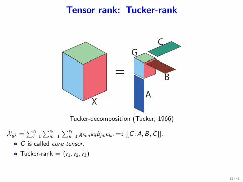
Tucker-decomposition (Tucker, 1966)
Xijk =∑r1
l=1
∑r2m=1
∑r3n=1 glmnailbjmckn =: [[G ;A,B,C ]].
G is called core tensor.
Tucker-rank = (r1, r2, r3)
12 / 41
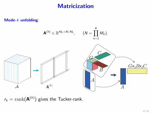
Matricization
Mode-k unfolding:
A(k) ∈ RMk×N/Mk , (N =K∏
k=1
Mk).
A A(k)
G
A
B
C
A
Gx2Bx3C
rk = rank(A(k)) gives the Tucker-rank.
13 / 41
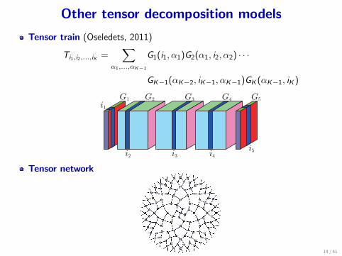
Other tensor decomposition models
Tensor train (Oseledets, 2011)
Ti1,i2,...,iK =∑
α1,...,αK−1
G1(i1, α1)G2(α1, i2, α2) · · ·
GK−1(αK−2, iK−1, αK−1)GK (αK−1, iK )
i2 i3 i4
i1
i5
G1 G2 G3 G4 G5
Tensor network
14 / 41
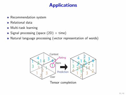
Applications
Recommendation system
Relational data
Multi-task learning
Signal processing (space (2D) × time)
Natural language processing (vector representation of words)
113122 24 2 42132412 3
234213 21 4113
2 4 4141 3
3213 2
User
Item
ContextRating
Prediction
Tensor completion
15 / 41
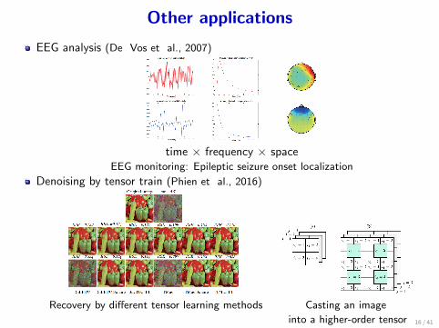
Other applications
EEG analysis (De Vos et al., 2007)
time × frequency × spaceEEG monitoring: Epileptic seizure onset localization
Denoising by tensor train (Phien et al., 2016)
Recovery by different tensor learning methods Casting an image
into a higher-order tensor 16 / 41
Outline
1 Introduction
2 Basics of low rank tensor decomposition
3 Nonparametric tensor estimationAlternating minimizationConvergence analysisReal data analysis: multitask learning
17 / 41
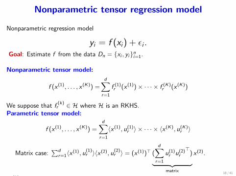
Nonparametric tensor regression model
Nonparametric regression model
yi = f (xi) + ϵi .Goal: Estimate f from the data Dn = {xi , yi}ni=1.
Nonparametric tensor model:
f (x (1), . . . , x (K)) =d∑
r=1
f (1)r (x (1))× · · · × f (K)r (x (K))
We suppose that f(k)r ∈ H where H is an RKHS.
Parametric tensor model:
f (x (1), . . . , x (K)) =d∑
r=1
⟨x (1), u(1)r ⟩ × · · · × ⟨x (K), u(K)r ⟩
Matrix case:∑d
r=1⟨x (1), u(1)r ⟩⟨x (2), u(2)r ⟩ = (x (1))⊤ (
d∑r=1
u(1)r u(2)r
⊤)︸ ︷︷ ︸
matrix
x (2).
(x (k))k is not necessarily an element of the Euclidean space.18 / 41

Application: Nonlinear recommendation
f (x (1), x (2)) = x (1)⊤Ax (2) =d∑
r=1
⟨x (1), u(1)r ⟩⟨u(2)
r , x (2)⟩
x (1): User feature,x (2): Movie feature.19 / 41
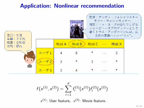
Application: Nonlinear recommendation
f (x (1), x (2)) =d∑
r=1
f (1)r (x (1))f (2)r (x (2))
x (1): User feature,x (2): Movie feature.19 / 41
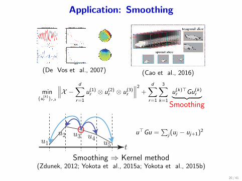
Application: Smoothing
(De Vos et al., 2007) (Cao et al., 2016)
min{u(k)
r }r,k
∥∥∥X − d∑r=1
u(1)r ⊗ u(2)r ⊗ u(3)r
∥∥∥2 + d∑r=1
3∑k=1
u(k)⊤r Gu(k)r︸ ︷︷ ︸Smoothing
tu1
u2 u3 u4u5
u⊤Gu =∑
j(uj − uj+1)2
Smoothing ⇒ Kernel method(Zdunek, 2012; Yokota et al., 2015a; Yokota et al., 2015b)
20 / 41
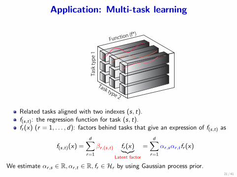
Application: Multi-task learning
Task type 1
Task type 2
Function (f*)
Related tasks aligned with two indexes (s, t).f(s,t): the regression function for task (s, t).fr (x) (r = 1, . . . , d): factors behind tasks that give an expression of f(s,t) as
f(s,t)(x) =d∑
r=1
βr ,(s,t) fr (x)︸︷︷︸Latent factor
=d∑
r=1
αr ,sαr ,t fr (x)
We estimate αr ,s ∈ R, αr ,t ∈ R, fr ∈ Hr by using Gaussian process prior.21 / 41
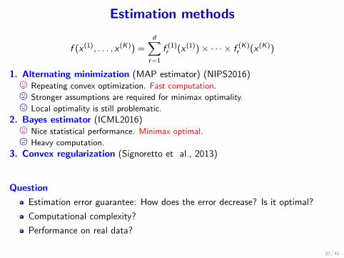
Estimation methods
f (x (1), . . . , x (K)) =d∑
r=1
f (1)r (x (1))× · · · × f (K)r (x (K))
1. Alternating minimization (MAP estimator) (NIPS2016), Repeating convex optimization. Fast computation./ Stronger assumptions are required for minimax optimality./ Local optimality is still problematic.
2. Bayes estimator (ICML2016), Nice statistical performance. Minimax optimal./ Heavy computation.
3. Convex regularization (Signoretto et al., 2013)
Question
Estimation error guarantee: How does the error decrease? Is it optimal?
Computational complexity?
Performance on real data?
22 / 41
Outline
1 Introduction
2 Basics of low rank tensor decomposition
3 Nonparametric tensor estimationAlternating minimizationConvergence analysisReal data analysis: multitask learning
23 / 41

Alternating minimization method
Update f(k)r for a chosen (r , k) while other components are fixed:
F ({f (k)r }r ,k) :=1
n
n∑i=1
(yi −
d∗∑r=1
K∏k=1
f (k)r (x(k)i )
)2
(Empirical error)
f (k)r ← argminf(k)r ∈H
{F (f (k)r |{f
(k′)r ′ }(r ′,k′) =(r ,k)) + λ∥f (k)r ∥2H
}.
The objective function is non-convex.
But it is convex w.r.t. one component f(k)r (kernel ridge regression).
It should converge to a local optimal (e.g. coordinate descent).
24 / 41
Reproducing Kernel Hilbert Space (RKHS)
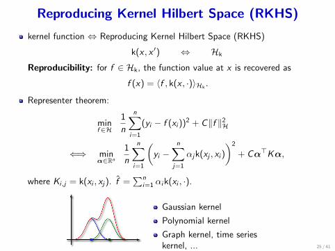
kernel function ⇔ Reproducing Kernel Hilbert Space (RKHS)
k(x , x ′) ⇔ Hk
Reproducibility: for f ∈ Hk, the function value at x is recovered as
f (x) = ⟨f , k(x , ·)⟩Hk.
Representer theorem:
minf∈H
1
n
n∑i=1
(yi − f (xi ))2 + C∥f ∥2H
⇐⇒ minα∈Rn
1
n
n∑i=1
(yi −
n∑j=1
αjk(xj , xi )
)2
+ Cα⊤Kα,
where Ki,j = k(xi , xj). f =∑n
i=1 αik(xi , ·).
Gaussian kernel
Polynomial kernel
Graph kernel, time serieskernel, ... 25 / 41
Outline
1 Introduction
2 Basics of low rank tensor decomposition
3 Nonparametric tensor estimationAlternating minimizationConvergence analysisReal data analysis: multitask learning
26 / 41
Complexity of the RKHS
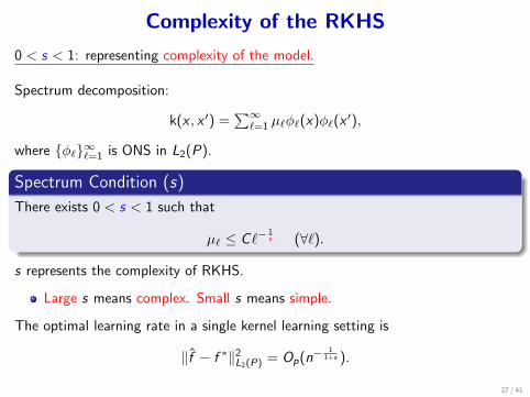
0 < s < 1: representing complexity of the model.
Spectrum decomposition:
k(x , x ′) =∑∞
ℓ=1 µℓϕℓ(x)ϕℓ(x′),
where {ϕℓ}∞ℓ=1 is ONS in L2(P).
Spectrum Condition (s)
There exists 0 < s < 1 such that
µℓ ≤ Cℓ−1s (∀ℓ).
s represents the complexity of RKHS.
Large s means complex. Small s means simple.
The optimal learning rate in a single kernel learning setting is
∥f − f ∗∥2L2(P) = Op(n− 1
1+s ).
27 / 41
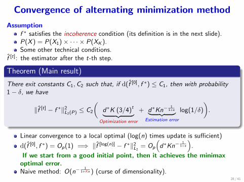
Convergence of alternating minimization method
Assumptionf ∗ satisfies the incoherence condition (its definition is in the next slide).P(X ) = P(X1)× · · · × P(XK ).Some other technical conditions.
f [t]: the estimator after the t-th step.
Theorem (Main result)
There exit constants C1,C2 such that, if d(f [0], f ∗) ≤ C1, then with probability1− δ, we have
∥f [t] − f ∗∥2L2(P) ≤ C2
(d∗K (3/4)t︸ ︷︷ ︸
Optimization error
+ d∗Kn−1
1+s︸ ︷︷ ︸Estimation error
log(1/δ)
).
Linear convergence to a local optimal (log(n) times update is sufficient)
d(f [0], f ∗) = Op(1) =⇒ ∥f [log(n)] − f ∗∥2L2= Op
(d∗Kn−
11+s
).
If we start from a good initial point, then it achieves the minimaxoptimal error.Naive method: O(n−
11+Ks ) (curse of dimensionality).
28 / 41

Details of technical conditions
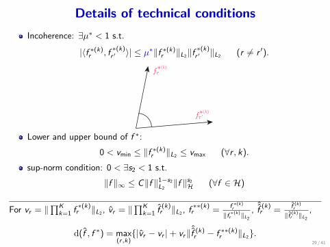
Incoherence: ∃µ∗ < 1 s.t.
|⟨f ∗(k)r , f∗(k)r ′ ⟩| ≤ µ∗∥f ∗(k)r ∥L2∥f
∗(k)r ′ ∥L2 (r = r ′).
fr*(k)
fr'*(k)
Lower and upper bound of f ∗:
0 < vmin ≤ ∥f ∗(k)r ∥L2 ≤ vmax (∀r , k).sup-norm condition: 0 < ∃s2 < 1 s.t.
∥f ∥∞ ≤ C∥f ∥1−s2L2∥f ∥s2H (∀f ∈ H)
For vr = ∥∏K
k=1 f∗(k)r ∥L2 , vr = ∥
∏Kk=1 f
(k)r ∥L2 , f
∗∗(k)r =
f ∗(k)r
∥f ∗(k)r ∥L2
, ˆf(k)r =
f (k)r
∥f (k)r ∥L2
,
d(f , f ∗) = max(r ,k){|vr − vr |+ vr∥ˆf (k)r − f ∗∗(k)r ∥L2}.
29 / 41
Details of technical conditions
Incoherence: ∃µ∗ < 1 s.t.
|⟨f ∗(k)r , f∗(k)r ′ ⟩| ≤ µ∗∥f ∗(k)r ∥L2∥f
∗(k)r ′ ∥L2 (r = r ′).
fr*(k)
fr'*(k)
Lower and upper bound of f ∗:
0 < vmin ≤ ∥f ∗(k)r ∥L2 ≤ vmax (∀r , k).sup-norm condition: 0 < ∃s2 < 1 s.t.
∥f ∥∞ ≤ C∥f ∥1−s2L2∥f ∥s2H (∀f ∈ H)
For vr = ∥∏K
k=1 f∗(k)r ∥L2 , vr = ∥
∏Kk=1 f
(k)r ∥L2 , f
∗∗(k)r =
f ∗(k)r
∥f ∗(k)r ∥L2
, ˆf(k)r =
f (k)r
∥f (k)r ∥L2
,
d(f , f ∗) = max(r ,k){|vr − vr |+ vr∥ˆf (k)r − f ∗∗(k)r ∥L2}.
29 / 41

Illustration of the theoretical result
True
Pred. Error
Emp. Error
True
Pred. Risk
Emp. Risk
True
Pred. Risk
Emp. Risk
Small sample Large sample
The predictive risk shapes like a convex function locally around the truefunction.
The empirical risk gets closer to the predictive one as the sample sizeincreases.
Technique: Local Rademacher complexity
30 / 41

Tools used in the proof
Rademacher complexityH: function space
Ex
[suph∈H
∣∣∣∣∣ 1nn∑
i=1
h(xi )︸ ︷︷ ︸Empirical error
− E[h]︸︷︷︸Predictive error
∣∣∣∣∣]
≤2Ex,σ
[suph∈H
∣∣∣∣∣1nn∑
i=1
σih(xi )
∣∣∣∣∣]≤ C√
n
where {σi}ni=1 are i.i.d. Rademacher random va-
riables (P(σi = 1) = P(σi = −1)).
Pred. RiskEmp. Risk
Uniform bound
Local Rademacher complexity + peeling device:Utilize strong convexity of the squared loss
Ex,σ
[suph∈H
| 1n∑n
i=1 σih(xi )|∥h∥L2 + λ
]≤ C
λ− s2
√n∨ λ− 1
2
n−1
1+s
Tighter around the true function
Pred. RiskEmp. Risk
Uniform bound31 / 41
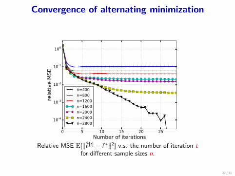
Convergence of alternating minimization
0 5 10 15 20 25
Number of iterations
10-4
10-3
10-2
10-1
100re
lati
ve M
SE
n=400
n=800
n=1200
n=1600
n=2000
n=2400
n=2800
Relative MSE E[∥f [t] − f ∗∥2] v.s. the number of iteration tfor different sample sizes n.
32 / 41
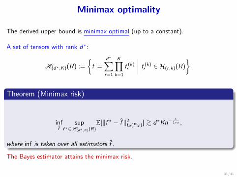
Minimax optimality
The derived upper bound is minimax optimal (up to a constant).
A set of tensors with rank d∗:
H(d∗,K)(R) :=
{f =
d∗∑r=1
K∏k=1
f (k)r
∣∣∣∣ f (k)r ∈ H(r ,k)(R)
}.
Theorem (Minimax risk)
inff
supf ∗∈H(d∗,K)(R)
E[∥f ∗ − f ∥2L2(PX )] ≳ d∗Kn−1
1+s ,
where inf is taken over all estimators f .
The Bayes estimator attains the minimax risk.
33 / 41
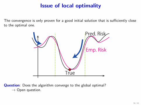
Issue of local optimality
The convergence is only proven for a good initial solution that is sufficiently closeto the optimal one.
True
Pred. Risk
Emp. Risk
Question: Does the algorithm converge to the global optimal?→ Open question.
34 / 41
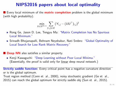
NIPS2016 papers about local optimality
■ Every local minimum of the matrix completion problem is the global minimum(with high probability).
minU∈RM×k
∑(i,j)∈E
(Yi,j − (UU⊤)i,j)2
Rong Ge, Jason D. Lee, Tengyu Ma: “Matrix Completion has No SpuriousLocal Minimum.”
Srinadh Bhojanapalli, Behnam Neyshabur, Nati Srebro: “Global Optimality ofLocal Search for Low Rank Matrix Recovery.”
■ Deep NN also satisfies a similar property.
Kenji Kawaguchi: “Deep Learning without Poor Local Minima.”(Essentially, the proof is valid only for linear deep neural network.)
Strictly saddle function: Every critical point has a negative curvature directionor is the global optimum.Trust region method (Conn et al., 2000), noisy stochastic gradient (Ge et al.,2015) can reach the global optimum for strictly saddle obj (Sun et al., 2015).
35 / 41
Outline
1 Introduction
2 Basics of low rank tensor decomposition
3 Nonparametric tensor estimationAlternating minimizationConvergence analysisReal data analysis: multitask learning
36 / 41
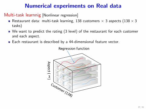
Numerical experiments on Real data
Multi-task learnnig [Nonlinear regression]
Restaurant data: multi-task learning, 138 customers × 3 aspects (138× 3tasks)
We want to predict the rating (3 level) of the restaurant for each customerand each aspect.
Each restaurant is described by a 44-dimensional feature vector.
37 / 41
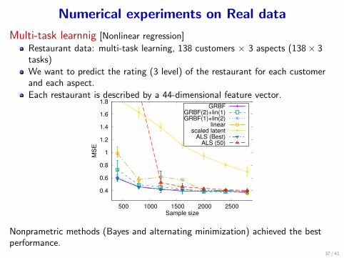
Numerical experiments on Real data
Multi-task learnnig [Nonlinear regression]
Restaurant data: multi-task learning, 138 customers × 3 aspects (138× 3tasks)We want to predict the rating (3 level) of the restaurant for each customerand each aspect.Each restaurant is described by a 44-dimensional feature vector.
0.4
0.6
0.8
1
1.2
1.4
1.6
1.8
500 1000 1500 2000 2500
MS
E
Sample size
GRBFGRBF(2)+lin(1)GRBF(1)+lin(2)
linearscaled latent
ALS (Best)ALS (50)
Nonprametric methods (Bayes and alternating minimization) achieved the bestperformance.
37 / 41
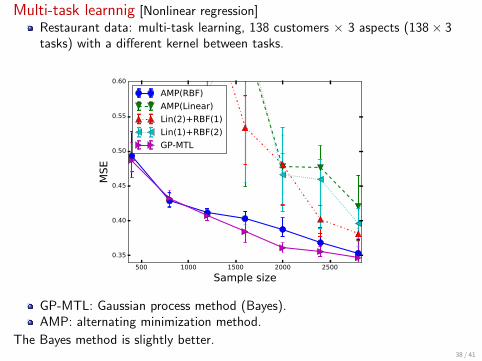
Multi-task learnnig [Nonlinear regression]Restaurant data: multi-task learning, 138 customers × 3 aspects (138× 3tasks) with a different kernel between tasks.
500 1000 1500 2000 2500
Sample size
0.35
0.40
0.45
0.50
0.55
0.60
MSE
AMP(RBF)
AMP(Linear)
Lin(2)+RBF(1)
Lin(1)+RBF(2)
GP-MTL
GP-MTL: Gaussian process method (Bayes).AMP: alternating minimization method.
The Bayes method is slightly better.38 / 41
Numerical experiments on Real data
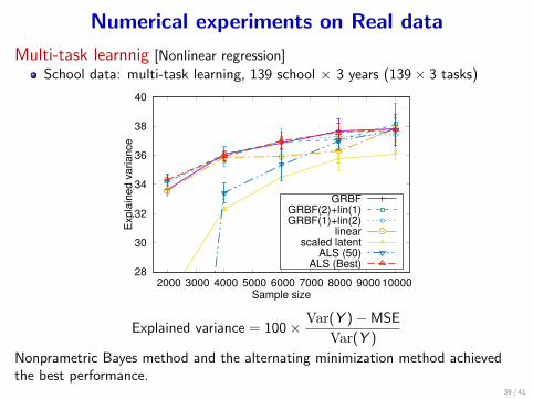
Multi-task learnnig [Nonlinear regression]
School data: multi-task learning, 139 school × 3 years (139× 3 tasks)
28
30
32
34
36
38
40
2000 3000 4000 5000 6000 7000 8000 9000 10000
Exp
lain
ed
va
ria
nce
Sample size
GRBFGRBF(2)+lin(1)GRBF(1)+lin(2)
linearscaled latent
ALS (50)ALS (Best)
Explained variance = 100× Var(Y )−MSE
Var(Y )
Nonprametric Bayes method and the alternating minimization method achievedthe best performance.
39 / 41

Online shopping sales prediction
Predict the online shopping (Yahoo! shopping) sales.
shop × item × customer (508 shops, 100 items)
Predict the number of certain items that a customer will buy in a shop.
A customer is represented by a feature vector.
We construct a kernel defined by the nearest neighbor graph between shops.
10
11
12
13
14
15
16
4000 6000 8000 10000 12000 14000
MS
E
Sample size
GP-MTL(cosdis)GP-MTL(cossim)
AMP(cosdis)AMP(cossim)
Figuur: Sales prediction of online shop. Comparison between different metrics betweenshops.
40 / 41
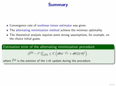
Summary
Convergence rate of nonlinear tensor estimator was given.
The alternating minimization method achieve the minimax optimality.
The theoretical analysis requires some strong assumptions, for example, onthe choice initial guess.
Estimation error of the alternating minimization procedure
∥f [t] − f ∗∥2L2(Π)≤ C
(dKn−
11+s + dK (3/4)t
).
where f [t] is the solution of the t-th update during the procedure.
41 / 41
Cao, W., Wang, Y., Sun, J., Meng, D., Yang, C., Cichocki, A., & Xu, Z. (2016).Total variation regularized tensor RPCA for background subtraction fromcompressive measurements. IEEE Transactions on Image Processing, 25,4075–4090.
Carroll, J. D., & Chang, J.-J. (1970). Analysis of individual differences inmultidimensional scaling via an n-way generalization of“ eckart-young”decomposition. Psychometrika, 35, 283–319.
Cohen, N., Sharir, O., & Shashua, A. (2016). On the expressive power of deeplearning: A tensor analysis. The 29th Annual Conference on Learning Theory(pp. 698–728).
Cohen, N., & Shashua, A. (2016). Convolutional rectifier networks as generalizedtensor decompositions. Proceedings of the 33th International Conference onMachine Learning (pp. 955–963).
Conn, A. R., Gould, N. I., & Toint, P. L. (2000). Trust region methods, vol. 1.Siam.
De Lathauwer, L. (2006). A link between the canonical decomposition inmultilinear algebra and simultaneous matrix diagonalization. SIAM journal onMatrix Analysis and Applications, 28, 642–666.
De Lathauwer, L., De Moor, B., & Vandewalle, J. (2004). Computation of thecanonical decomposition by means of a simultaneous generalized schurdecomposition. SIAM journal on Matrix Analysis and Applications, 26, 295–327.
41 / 41
De Vos, M., Vergult, A., De Lathauwer, L., De Clercq, W., Van Huffel, S.,Dupont, P., Palmini, A., & Van Paesschen, W. (2007). Canonicaldecomposition of ictal scalp eeg reliably detects the seizure onset zone.NeuroImage, 37, 844–854.
Ge, R., Huang, F., Jin, C., & Yuan, Y. (2015). Escaping from saddlepoints—online stochastic gradient for tensor decomposition. Proceedings ofThe 28th Conference on Learning Theory (pp. 797–842).
Harshman, R. A. (1970). Foundations of the PARAFAC procedure: Models andconditions for an “explanatory” multi-modal factor analysis. UCLA WorkingPapers in Phonetics, 16, 1–84.
Hitchcock, F. L. (1927). Multilple invariants and generalized rank of a p-waymatrix or tensor. Journal of Mathematics and Physics, 7, 39–79.
Kanagawa, H., Suzuki, T., Kobayashi, H., Shimizu, N., & Tagami, Y. (2016).Gaussian process nonparametric tensor estimator and its minimax optimality.Proceedings of the 33rd International Conference on Machine Learning(ICML2016) (pp. 1632–1641).
Leurgans, S., Ross, R., & Abel, R. (1993). A decomposition for three-way arrays.SIAM Journal on Matrix Analysis and Applications, 14, 1064–1083.
Mu, C., Huang, B., Wright, J., & Goldfarb, D. (2014). Square deal: Lowerbounds and improved relaxations for tensor recovery. Proceedings of the 31thInternational Conference on Machine Learning (pp. 73–81).
41 / 41
Oseledets, I. V. (2011). Tensor-train decomposition. SIAM Journal on ScientificComputing, 33, 2295–2317.
Phien, H. N., Tuan, H. D., Bengua, J. A., & Do, M. N. (2016). Efficient tensorcompletion: Low-rank tensor train. arXiv preprint arXiv:1601.01083.
Signoretto, M., Lathauwer, L. D., & Suykens, J. A. K. (2013). Learning tensors inreproducing kernel Hilbert spaces with multilinear spectral penalties. CoRR,abs/1310.4977.
Sun, J., Qu, Q., & Wright, J. (2015). When are nonconvex problems not scary?arXiv preprint arXiv:1510.06096.
Suzuki, T. (2015). Convergence rate of Bayesian tensor estimator and its minimaxoptimality. Proceedings of the 32nd International Conference on MachineLearning (ICML2015) (pp. 1273–1282).
Tomioka, R., & Suzuki, T. (2013). Convex tensor decomposition via structuredschatten norm regularization. Advances in Neural Information ProcessingSystems 26 (pp. 1331–1339). NIPS2013.
Tomioka, R., Suzuki, T., Hayashi, K., & Kashima, H. (2011). Statisticalperformance of convex tensor decomposition. Advances in Neural InformationProcessing Systems 24 (pp. 972–980). NIPS2011.
Tucker, L. R. (1966). Some mathematical notes on three-mode factor analysis.Psychometrika, 31, 279–311.
41 / 41
Yokota, T., Zdunek, R., Cichocki, A., & Yamashita, Y. (2015a). Smoothnonnegative matrix and tensor factorizations for robust multi-way data analysis.Signal Processing, 113, 234–249.
Yokota, T., Zhao, Q., & Cichocki, A. (2015b). Smooth parafac decomposition fortensor completion. arXiv preprint arXiv:1505.06611.
Zdunek, R. (2012). Approximation of feature vectors in nonnegative matrixfactorization with gaussian radial basis functions. International Conference onNeural Information Processing (pp. 616–623).
Zheng, Q., & Tomioka, R. (2015). Interpolating convex and non-convex tensordecompositions via the subspace norm. Advances in Neural InformationProcessing Systems (pp. 3088–3095).
41 / 41


![[Włodzimierz Greblicki; M Pawlak] Nonparametric System Identification](https://img.pdfslide.tips/doc/110x75/577c7c091a28abe05499073c/wlodzimierz-greblicki-m-pawlak-nonparametric-system-identification.jpg)