Embed Size (px)
Citation preview
Nontopological Solitons
in a Spontaneously Broken U(1) Gauge Theory
(対称性が自発的に破れたU(1)ゲージ理論に於ける
ノントポロジカルソリトン)
Tatsuya Ogawa(小川 達也)

Nontopological Solitonsin a Spontaneously Broken U(1) Gauge Theory
(対称性が自発的に破れたU(1)ゲージ理論に於ける
ノントポロジカルソリトン)
Department of Mathematics and Physics,
Graduate School of Science
令和元年度
Tatsuya Ogawa
(小川 達也)

Abstract
We construct spherically symmetric nontopological solitons, Q-balls, in
a system consists of a complex matter scalar field, a U(1) gauge field, and
a complex Higgs scalar field with a potential that causes the spontaneous
symmetry breaking. This is a generalized system based on the model by
Friedberg, Lee, and Sirlin.
In the Q-balls of our system, the U(1) charge densities are induced by
both the complex scalar matter field and the complex Higgs scalar fields.
Owing to the Higgs mechanism the gauge field aquires a mass, that it me-
diates short-range force in the vacuum state. As a result, influence of the
charge induced by the complex scalar matter field is limited in a finite range
of distance. In other words, the charge induced by the complex scalar matter
field should be screened by some appropriate configuration of the complex
Higgs scalar field.
If we restrict the system stationary and spherically symmetric, the sys-
tem considered in this paper is analogous to a dynamical system of a particle
in three dimensions, and then a configuration of the fields can be interpreted
as a motion of the particle. There are some stationary points in the dynam-
ical system, whose one of them corresponds to the vacuum. We find bounce
solutions that describe large Q-balls: a particle starts from a stationary point
traverses toward the vacuum stationary point. By numerical calculations,
we show that Q-balls which can be interpreted as bounce solutions have the
following properties: (i) the size can be arbitrarly large, (ii) energetically
stable, and (iii) charge is screened everywhere.
2
Acknowledgements
I am very grateful to Prof. Hideki Ishihara for his continuous encouragement,
meaningful discussions, and genuine support throughout my post graduate
study. Also, I would like to thank to Prof. Ken-ichi Nakao, Prof. Hiroshi
Itoyama, Prof. Nobuhito Maru, and Prof. Sanefumi Moriyama for valu-
able suggestions. It is also my pleasure to thank all of the members of
research group for theoretical astrophysics, particle physics, and mathemat-
ical physics in Osaka City University, especially, Dr. Ryusuke Nishikawa,
Dr. Hirotaka Yoshino, Dr. Yoshiyuki Morisawa, Dr. Ryotaku Suzuki, Dr.
Hiroyuki Negishi, Dr. Atsuki Masuda. I am thankful to Prof. Masaki
Arima, Prof. Nobuyuki Sakai, and Dr. Masato Minamitsuji for helpful ad-
vice. Finally, I would like to thank my family for trusting and supporting
me.
3
Contents
1 Introduction 6
2 U(1) Gauge theory and Higgs mechanism 9
2.1 Global symmetry . . . . . . . . . . . . . . . . . . . . . . . . . 9
2.2 Local symmetry . . . . . . . . . . . . . . . . . . . . . . . . . . 10
2.3 Higgs Mechanism . . . . . . . . . . . . . . . . . . . . . . . . . 10
3 Charge Screening of Extended Sources in a Spontaneously
Symmetry Broken System 12
3.1 Charge screening with a Proca field . . . . . . . . . . . . . . . 12
3.2 Basic System with the spontaneous symmetry breaking . . . 14
3.3 Spherically symmetric model . . . . . . . . . . . . . . . . . . 16
3.4 Numerical Calculations . . . . . . . . . . . . . . . . . . . . . 18
3.4.1 Gaussian distribution source . . . . . . . . . . . . . . 18
3.4.2 Homogenious ball source . . . . . . . . . . . . . . . . . 23
4 Q-balls in a Spontaneously Broken U(1) Gauge Theory 27
4.1 Q-balls and gauged Q-balls in a coupled two scalar fields model 27
4.2 Basic Model . . . . . . . . . . . . . . . . . . . . . . . . . . . . 28
4.3 Numerical Calculations . . . . . . . . . . . . . . . . . . . . . 31
4.4 Homogeneous ball solutions . . . . . . . . . . . . . . . . . . . 34
4.5 Stability . . . . . . . . . . . . . . . . . . . . . . . . . . . . . . 38
5 Summary 41
Appendicies 45
Appendix A Charge Screning of a Point source . . . . . . . . . . 45
A.1 Asymptotic behaviors for the point source . . . . . . . 45
A.2 Distant region . . . . . . . . . . . . . . . . . . . . . . 46
4
A.3 Numerical calculations . . . . . . . . . . . . . . . . . . 47
Appendix B Approximate solutions for the Gaussian distribu-
tion sources . . . . . . . . . . . . . . . . . . . . . . . . . . . . 51
Appendix C Approximate solutions for the homogeneous ball
sources . . . . . . . . . . . . . . . . . . . . . . . . . . . . . . . 53
Appendix D Energy-Momentum Tensor of the System . . . . . . 55
Appendix E Other bounce solutions . . . . . . . . . . . . . . . . 56
E.1 Stationary Points of the System and Bounce Solutions 56
E.2 Numerical calculations . . . . . . . . . . . . . . . . . . 56
5
Chapter 1
Introduction
In 1834, John Scott Russell observed that a solitary wave were created and
propagated on a canal. The wave has the following characteristic properties:
velocity and shape of the wave do not change while it propergates over a
long distance. Since the wave behaves like a particle, such solitary waves
are called solitons.
The soliton solutions appear in various research fields of science: op-
tics, biology, and field theories in physics. The solitons in the field theories
are classical solutions to nonlinear field equations, where the each energy
is localized in a finite spatial region. The solitons are divided into two
types: topological solitons, and nontopological solitons. The former are ho-
motopically distinct solutions from the vacuum solution, namely, field con-
figurations with topological charge, which are invariant under continuous
deformations of the fields with fixed boundary conditions. The topologi-
cal solitons cannot relax to the zero energy configuration due to conserved
topological quantities. For example, domain walls, cosmic strings [1], and
’t Hooft-Polyakov-monopoles [2] are topological solitons [3]. The latter,
nontopological soliton, represent field configurations which have the lowest
energy for fixed conserved charge in global U(1)-invariant theories, and can
be interpreted as bound states of bosonic particles.
The first nontopological soliton solutions to a nonlinear scalar field the-
ory was first found by Rosen in 1968 [4, 5]. In 1976, Friedberg, Lee and
Sirlin [6] introduced the nontopological solitons in a coupled system of a
complex scalar field and a real scalar field with a potential that causes the
spontaneous Z2 symmetry breaking. Some years later, the simplest example
of the nontopological solitons was proposed in a system of a self-interacting
6
single complex scalar field by Coleman in 1985 [7]. He called the spherically
symmetric nontopological solitons Q-balls1. The models with a single scalar
field are assumed to have complicated self-interactions, e.g., third or sixth
order potentials, or non-polynomial potentials, for the existence of Q-balls.
On the other hand, in the models with two scaler fields, more natural poten-
tials, e.g., forth order potentials, and interaction between two scalar fields
are assumed.
The Q-balls have been widely investigated in a context of cosmologies
and astrophysics. A. Kusenko constructed Q-balls in a minimal supersym-
metric standard model that include global U(1) symmetries in 1997 [8, 9].
It is known that a Q-ball can be a candidate of dark matter of the Universe
[11, 12, 13, 14, 15, 16] and a source for a baryogenesis [17, 18, 10, 19].
If taking a gravity into account, the stable Q-balls can be boson stars.
[36, 37, 38, 39, 40, 41]. The boson stars have been investigated as a can-
didate of central core of galaxies [40], and a source of gravitational wave
[42].
Genelalization of the Q-balls by requiring a local U(1)-invariance, achieved
by a U(1) gauge field, so-called gauged Q-balls, was first studied by K.M.
Lee, J.A. Stein-Schabes, R. Watkins and L.M. Widrow in 1988 [20] based
on the system by Coleman, and many works follow it [21, 22]. Their system
consisis of a complex scalar field coupled to a U(1) gauge field. On the other
hand, gauged Q-balls based on the system by Friedberg, Lee, and Sirlin was
proposed in 1991 [21]. This system consists of a real scalar fields with a po-
tential that causes spontaneously the Z2 symmetry breaking and a complex
scalar field coupled to a U(1) gauge field. The both types of the gauged Q-
balls have significant properties compared with the nongauged Q-balls. For
example, nongauged Q-balls with arbitrary large charge are allowed, while
gauged Q-balls have upper bound of charge because of the Coulomb repul-
sive force mediated by the gauge field. Another genalirized Q-balls with
a fermionic field called fermionic Q-balls are proposed [49, 50, 51, 52]. In
this case, a large fermionic soliton is hardly produced because of the Pauli
exclusion principle.
In this paper, we generalize the gauged Q-balls based on the Friedberg,
Lee, and Sirlin system. We consider a system consist of a complex matter
scalar field, a U(1) gauge field, and a complex Higgs scalar field with a
1Hereafter, we call a spherically symmetric nontopological soliton a Q-ball, in short.
7
potential that causes the spontaneous symmetry breaking. The local U(1) ×global U(1) symmetry breaks to the global U(1) symmetry through the Higgs
mechanism. We show the existence of Q-balls as stationary and spherically
symmetric solutions in the model that has simple natural interaction terms.
Then, this work would suggest Q-balls can appear in a wide class of gauge
theories.
In our system of the gauged Q-balls, the U(1) charge densities are in-
duced by both the complex scalar matter field, and the complex Higgs scalar
fields. Owing to the Higgs mechanism the gauge field which aquires a mass
mediates a short-range force in the vacuum state. As a result, influence of
the charge induced by the complex scalar matter field is limited in a finite
range of distance. In other words, the charge induced by the complex scalar
matter field should be screened by some appropriate configuration of the
complex Higgs scalar field.
If we restrict the system stationary and spherically symmetric, the sys-
tem considered in this paper is analogous to a dynamical system of a particle
in three dimensions, and then a configuration of the fields can be interpreted
as a motion of the particle.
The dynamical system of the particle has some unstable stationary points.
One of the stationary point corresponds to the vacuum. The particle that
travels toward the vacuum stationary point describes a Q-ball solution. We
construct Q-balls by solving the dynamical system numerically.
If the particle stays an initial stationary point long time, and travels to
the vacuum stationary point quickly, the size of the corresponding Q-ball is
large. We show that a Q-ball that has the following properties is allowed:
(i) the size can be arbitrarly large, (ii) energetically stable, (iii) charge is
screened everywhere. It would be preferable properties for a candidate of
dark matter in the universe.
The paper is organized as follows. In Chap.2, we review a U(1) gauge
theory and a Higgs mechanism, and define a total charge screening used in
this paper. In Chap.3, we investigate charge screening in a system consists
of a complex Higgs scalar field and a U(1) gauge field with a external source
charge. In Chap.4, we construct numerical solutions of Q-ball in our system
and investigate their properties. In Chap.5, we summarize the paper.
8
Chapter 2
U(1) Gauge theory and
Higgs mechanism
2.1 Global symmetry
First, we consider the Lagrangian consisits of a complex scalar filed with
mass m given by
L = −(∂µϕ)∗(∂µϕ)−m2ϕ∗ϕ. (2.1)
This Largangian is invariant under a global U(1) transformation
ϕ(t, x) → ϕ′(t, x) = eiγϕ(t, x), (2.2)
where γ is an arbitrary constant. This corresponds to a phase rotation of
the complex scalar field in an inner space. “Global” means that the trans-
formation does not depend on spacetime coordinate (x, t). If Lagrangian
has this symmetry, the four-current density defined as
jµ := i (ϕ∗(∂µϕ)− ϕ(∂µϕ)∗) , (2.3)
is conserved, namely, ∂µjµ = 0 is satisfied. Consequently, the charge defined
by
Q :=
∫jtd3x, (2.4)
is conserved.
9
2.2 Local symmetry
Next, we consider that a transformation that depends on spacetime coordi-
nate (t, x) as
ϕ(t, x) → ϕ′(t, x) = eiχ(t,x)ϕ(t, x). (2.5)
This is called local U(1) transformation. In this case, (2.1) is not invariant
under (2.5). We require that the Lagrangian is invariant under local U(1)
transformation. A vector field Aµ(t, x) should be introduced and trans-
formed by
Aµ(t, x) → Aµ(t, x) = Aµ(t, x) + e−1∂µχ(t, x), (2.6)
where e is a coupling constatnt between the vector and the complex scalar
fields. This vector field is called U(1) gauge field. By introducing the gauge
field, the Lagrangian (2.1) is changed to
L = −(Dµϕ)∗(Dµϕ)− 1
2m2ϕ∗ϕ− 1
4FµνF
µν , (2.7)
where
Dµϕ := ∂µϕ− ieAµϕ, (2.8)
Fµν := ∂µAν − ∂νAµ (2.9)
are the covariant derivative and the field strength of a U(1) gauge field
Aµ respectively. Owing to the local U(1) symmetry, a four-current density
defined by
jµ := ie ϕ∗(Dνϕ)− ϕ(Dνϕ)∗ , (2.10)
and therefore the charge (2.4) are conserved.
2.3 Higgs Mechanism
In the previous sections, we introduced U(1) gauge symmetry. However,
assuming the gauge symmetry to the Lagrangian, we can not introduce a
mass term of the gauge field explicitly in the Lagrangian. In fact, the mass
term of the gauge field breaks the gauge symmetry as
m2AAµA
µ = m2AA
′µA
′µ. (2.11)
10
However, it is well known that the weak gauge boson have finite mass exper-
imentally. This problem was solved by using idea of spontaneous symmetry
breaking. The gauge field acquire the mass in symmetry breaking vacuum
naturally.
We consider a Lagrangian of the complex scalar field and the gauge field
given by
L = −(Dµϕ)∗(Dµϕ)− λ
4(ϕ∗ϕ− η2)2 − 1
4FµνF
µν , (2.12)
where λ and η are positive constants. Minima of the potential, say ϕ0(x),
are degenerate infinitely as given by
ϕ0(x) = ηeiθ(x), (2.13)
where θ is an arbitrary function. Without loss of generality, we can choose
θ = 0. Expanding small perturbation of the complex scalar field around
ϕ0 = η by
ϕ = η +1√2φ1 + iφ2
∼(η +
1√2φ1
)ei 1√
2ηφ2 , (2.14)
and choosing the gauge in (2.5), which is called unitary gauge,
χ(x) = − 1√2ηφ2, (2.15)
we can transform the complex scalar field by
ϕ′(x) = η +1√2φ1, (2.16)
where φ1 is a real scalar field. Substituting (2.16) into (2.12), we can rewrite
the Lagrangian as
L = −1
2(∂µφ1)(∂
µφ1)−1
2m2ϕφ
21 −
1
4FµνF
µν − 1
2m2AAµA
µ +O(φ31, A
3µ),
(2.17)
where mϕ :=√λη is a mass of the real scalar field. This Lagrangian is not
invariant under the local U(1) transformations, namely, symmetry is broken
spontaneously. As a result, the gauge field acquire the mass mA :=√2eη.
The scheme is called the Higgs mechanism.
11
Chapter 3
Charge Screening of
Extended Sources in a
Spontaneously Symmetry
Broken System
In this chapter, we introduce a total charge screening by classical solutions
in field theories. The total charge screening by the fields are proposed in
1970s to 1980s which is motivated to explain color confinment in quantum
chromodynamics [53, 54, 55, 56].
3.1 Charge screening with a Proca field
In this section we show that if massive vector field, Proca field, mediate the
interaction between charge, the charge screening should occur.
We consider a Proca field theory with an external source described by
the Lagrangian density
L = −1
4FµνF
µν − 1
2m2AAµA
µ − eAµJµ , Fµν := ∂µAν − ∂νAµ (3.1)
where Jµ is the external source.
The energy of the system is given by
E =
∫d3x
(1
2
(EiE
i +BiBi))
, (3.2)
12
where Ei := Fi0, Bi := 1/2ϵijkFjk, and i denotes spatial index. In the
vacuum state, which minimizes the energy (3.2), Aµ should take the form
Aµ = ∂µθ(x), (3.3)
where θ(x) is an arbitrary function.
By varying (3.1) with respect to Aµ, we obtain the equations of motion
∂µFµν = m2
AAν + eJν . (3.4)
We can interpret the right-hand side of (3.4) as the source of the Proca field.
We consider a static point source in the form
J t = δ3(r), and J i = 0, (3.5)
where t and r are the time and the radial coordinates. We also assume that
the fields are spherically symmetric and static in the form,
At = At(r), and Ai = 0. (3.6)
We impose that the Proca field should be in the vacuum state at infinity
At → 0. (3.7)
Substituting (3.6) into (3.4), we obtain
d2Atdr2
+2
r
dAtdr
= m2AAt − eδ3(r), (3.8)
and solving (3.8), we get
At(r) =e
4πrexp(−mA r). (3.9)
Therefore, in the vacuum state, the Proca field decays exponentially with
the mass scale. Then the influence of the source charge by the massive vector
field is limited in a finite range of distance.
From another point of view, we reinterpret the solution (3.9). Integrating
(3.8), we get
limr→∞
4πr2A′t = 4π
∫ ∞
0r2 ρind(r)− ρext(r) dr
: = Qind +Qext, (3.10)
13
where ρind := m2AAt is a charge density induced by the vector field and
ρext := eδ3(r), and Qind and Qext are total charge by the vector field and
the external source respectively. Substituting (3.9) into (3.10), we get
Qind +Qext = 0. (3.11)
This means that the charge of the external source is totally screened by the
counter charge of the vector field. From (3.10), At should decay faster than
r−1 for the total charge screening.
3.2 Basic System with the spontaneous symmetry
breaking
In the previous sections, it is shown that if a vector field have a mass,
the total screening of an external source occurs. On the other hand we
showed that a gauge field, vector field, can acquire a mass through the
Higgs mechanism in Chap.2. Therefore, we expect that if an external source
exist in abelian Higgs model, the source charge should be screened through
the Higgs mechanism.
We consider an abelian Higgs system described by the Lagrangian den-
sity
L = −(Dµϕ)∗(Dµϕ)− V (ϕ)− 1
4FµνF
µν , (3.12)
where Fµν := ∂µAν − ∂νAµ is the field strength of a U(1) gauge field Aµ,
and ϕ is a complex Higgs scalar field with the potential
V (ϕ) =λ
4(ϕ∗ϕ− η2)2, (3.13)
where λ and η are positive constants soliton. The Higgs field ϕ couples to
the gauge field by the covariant derivative given by
Dµϕ := ∂µϕ− ieAµϕ, (3.14)
where e is a coupling constant. The Lagrangian density (3.12) is invariant
under local U(1) gauge transformations,
ϕ(x) → ϕ′(x) = eiχ(x)ϕ(x), (3.15)
Aµ(x) → A′µ(x) = Aµ(x) + e−1∂µχ(x), (3.16)
14
where χ(x) is an arbitrary function.
The energy of the system is given by
E =
∫d3x
(|Dtϕ|2 + (Diϕ)
∗(Diϕ) + V (ϕ) +1
2
(EiE
i +BiBi))
, (3.17)
where Ei := Fi0, Bi := 1/2ϵijkFjk, and i denotes spatial index. In the
vacuum state, which minimizes the energy (3.17), ϕ and Aµ should take the
form
ϕ = ηeiθ(x) and Aµ = e−1∂µθ, (3.18)
where θ is an arbitrary function. Equivalently, eliminating θ we have
ϕ∗ϕ = η2 and Dµϕ = 0. (3.19)
After the Higgs scalar field takes the vacuum expectation value η, the gauge
field Aµ absorbing the Nambu-Goldstone mode, the phase of ϕ, forms a
massive vector field with the mass mA =√2eη, and the real scalar field
that denotes a fluctuation of the amplitude of ϕ around η acquires the mass
mϕ =√λη.
In order to study the charge screening, adding an extremal source cur-
rent, Jµ, coupled with Aµ to the original Lagrangian (3.12), we consider the
action1
S =
∫d4x
(−(Dµϕ)
∗(Dµϕ)− λ
4(ϕ∗ϕ− η2)2 − 1
4FµνF
µν − eAµJµ
).
(3.20)
By varying (3.20) with respect to ϕ∗ and Aµ, we obtain the equations of
motion
DµDµϕ− λ
2ϕ(ϕ∗ϕ− η2) = 0, (3.21)
∂µFµν = ejνind + eJν , (3.22)
where jνind is the gauge invariant current density that consists of ϕ and Aµ
defined by
jνind := i (ϕ∗(∂ν − ieAν)ϕ− ϕ(∂ν + ieAν)ϕ∗) . (3.23)1The case of vanishing potential, V (ϕ) = 0, in which the symmetry does not break,
is studied in ref.[53], and the case V (ϕ) = 12m2|ϕ|2, in which partial screening occurs, is
studied in ref.[54].
15
3.3 Spherically symmetric model
We consider a spherically symmetric and static external source in the form
eJ t = ρext(r), and eJ i = 0, (3.24)
where t and r are the time and the radial coordinates. We also assume that
the fields are spherically symmetric and stationary in the form,
ϕ = eiωtf(r), (3.25)
At = At(r), and Ai = 0, (3.26)
where ω is a constant, and f(r) is a real function of r. By using the gauge
transformation (3.15) and (3.16) to incorporate the phase rotation of ϕ, i.e.,
Nambu-Goldstone mode, with At, we introduce a new variable α(r) as
α(r) := At(r)− e−1ω. (3.27)
The charge density induced by the fields ϕ and Aµ defined by (3.23) is
written as
ρind := ejtind = −2e2f2α. (3.28)
Substituting (3.24) - (3.27) into (3.21) and (3.22), we obtain
d2f
dr2+
2
r
df
dr+ e2fα2 − λ
2f(f2 − η2) = 0, (3.29)
d2α
dr2+
2
r
dα
dr+ ρind(r) + ρext(r) = 0. (3.30)
Using the ansatz (3.25) and (3.26), we rewrite the energy (3.17) for the
symmetric system as
E = 4π
∫ ∞
0r2ϵ(r)dr, (3.31)
ϵ := ϵKin + ϵElast + ϵPot + ϵES, (3.32)
where
ϵKin := |Dtϕ|2 = e2f2α2, ϵElast := (Diϕ)∗(Diϕ) =
(df
dr
)2
, (3.33)
ϵPot := V (ϕ) =λ
4(f2 − η)2, ϵES :=
1
2EiE
i =1
2
(dα
dr
)2
, (3.34)
16
are density of kinetic energy, elastic energy, potential energy, and electro-
static energy, respectively.
We consider two extended source cases separately. As the extended
source cases, we discuss Gaussian distribution sources and homogeneous
ball sources. The both are smoothly distributed and have finite supports.
The charge density of the Gaussian distribution source is given by
ρext(r) = ρ0 exp
[−(r
rs
)2], (3.35)
where rs is the width of the extended source. The total external charge is
assumed to be normalized as
4π
∫ ∞
0r2ρext(r)dr = q, (3.36)
then the central density ρ0 is given by
ρ0 =q
π3/2 r3s. (3.37)
In the limit rs → 0, the charge density (3.35) with (3.37) reduces to the
point source case2.
The charge density of the homogeneous ball considered in this paper is
given by
ρext(r) =ρ02
[tanh
(rs − r
ζs
)+ 1
], (3.38)
where rs is the radius of the external source, and ζs is the thickness of surface
of the ball. We assume rs ≫ ζs so that the charge density within the radius
rs is almost constant value ρ0. Then, the total external charge is (4π/3)r3sρ0
in this case.
We impose boundary conditions so that the fields are regular at the
origin. The regularity conditions for the spherically symmetric fields at the
origin are
df
dr→ 0 ,
dα
dr→ 0 as r → 0. (3.39)
The energy density at the origin is finite for finite central values of f and α
. At infinity, the fields should be in the vacuum state, which minimizes ϵ in
(3.32). Therefore, we impose the conditions
f → η , α→ 0 as r → ∞. (3.40)2In the cases of a point source is discussed in Appendix A.
17
3.4 Numerical Calculations
We use the relaxation method to obtain numerical solutions to the coupled
ordinary differential equations (3.29) and (3.30). In numerics, hereafter,
we set η = 1, and scale the radial coordinate r as r → ηr, and scale the
functions f , α as f → η−1f , α→ η−1α, respectively.
3.4.1 Gaussian distribution source
For the first example of smoothly extended source, we consider the external
charge density given by the Gaussian distribution (3.35). As the boundary
conditions, we impose the regularity conditions (3.39) at the origin, and the
vacuum condition (3.40) at infinity.
For the extended external sources, the behaviors of f and α do not
depend critically on the value of κ := eq/(4π) unlike the point source case.
So, we concentrate on the case q = 1. We set e = 1/√2 and λ = 1 so that
rϕ := m−1ϕ = 1 and rA := m−1
A = 1, and perform numerical calculation with
several values of rs that denotes the thickness of the external source.
Field configurations
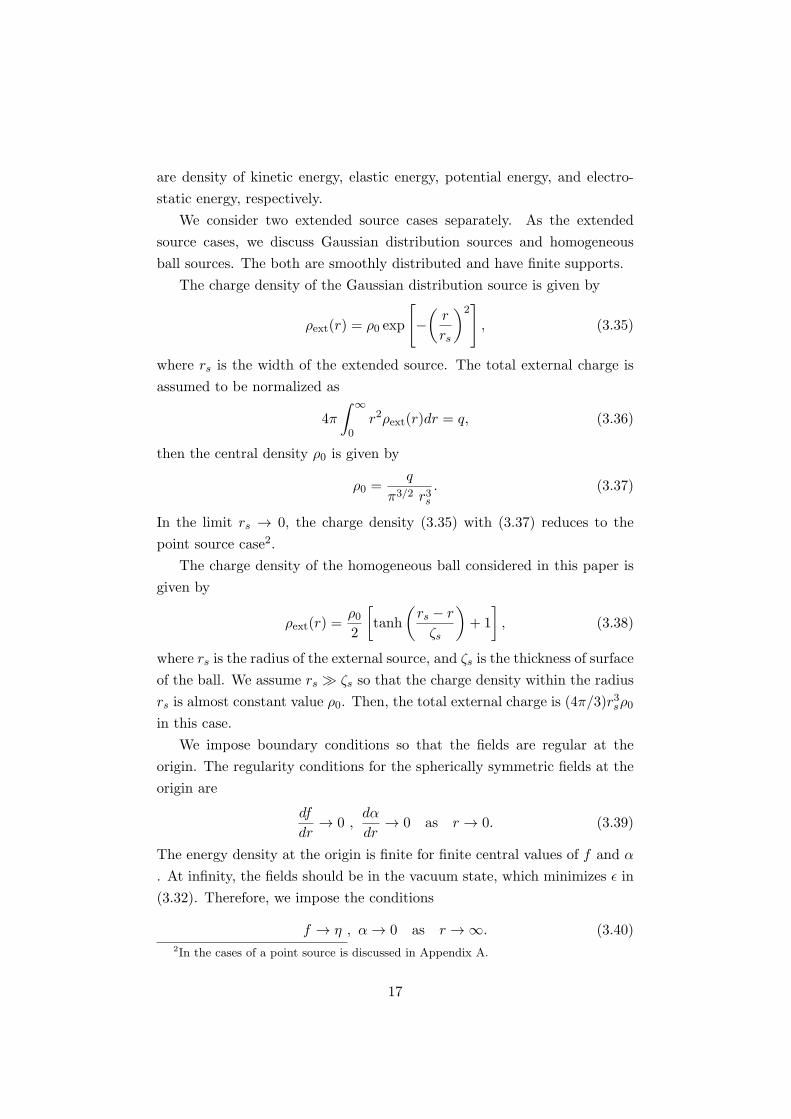
By numerical calculations, we show typical behaviors of the function f and
α with the external charge density ρext in the cases of rs = 0.1, 1, 10, and 100
in Fig.3.1. We see that the function f and α change in their shapes with rs.
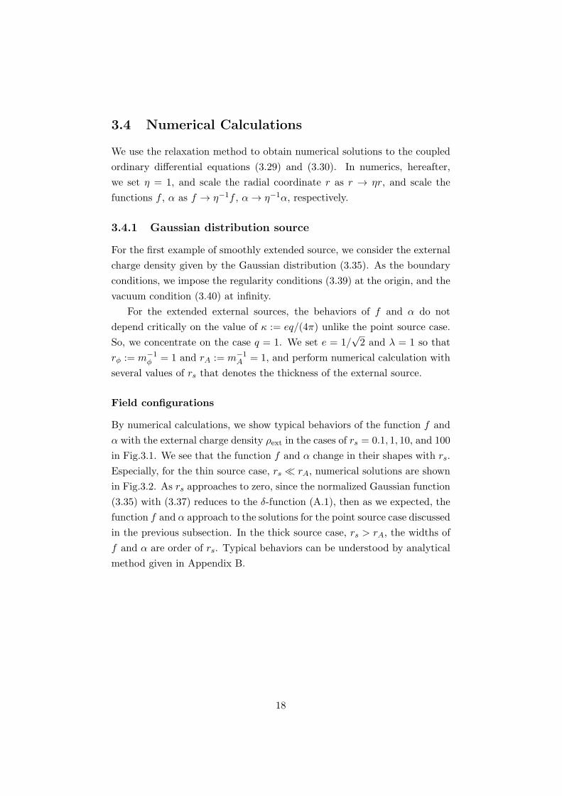
Especially, for the thin source case, rs ≪ rA, numerical solutions are shown
in Fig.3.2. As rs approaches to zero, since the normalized Gaussian function
(3.35) with (3.37) reduces to the δ-function (A.1), then as we expected, the
function f and α approach to the solutions for the point source case discussed
in the previous subsection. In the thick source case, rs > rA, the widths of
f and α are order of rs. Typical behaviors can be understood by analytical
method given in Appendix B.
18
102*( f-η)/(ρ0/η2)α/(ρ0/η
2)
ρext/ρ0
0.0 0.5 1.0 1.5 2.0 2.5 3.00.000
0.002
0.004
0.006
0.008
0.010
η r
rs=0.1
102*( f-η)/(ρ0/η2)α/(ρ0/η
2)
ρext/ρ0
0 2 4 6 8 100.0
0.2
0.4
0.6
0.8
1.0
η r
rs=1.0
102*( f-η)/(ρ0/η2)α/(ρ0/η
2)
ρext/ρ0
0 10 20 30 40 500.0
0.2
0.4
0.6
0.8
1.0
η r
rs=10
102*( f-η)/(ρ0/η2)α/(ρ0/η
2)
ρext/ρ0
0 100 200 300 400 5000.0
0.2
0.4
0.6
0.8
1.0
η r
rs=100
Figure 3.1: Numerical solutions in the case of Gaussian distribution
sources. Behaviors of f(r) and α(r) for rs = 0.1, 1, 10, 100 are drawn
together with ρext as functions of r. In the case of rs = 100, α(r)
coincides with ρext (see the lower right panel).
ρext=qδ3(r)rs=0.01
rs=0.1
rs=1.0
-7 -6 -5 -4 -3 -2 -1 00.000
0.005
0.010
0.015
0.020
loge[ηr]
loge[f/η]
ρext=qδ3(r)
rs=0.01
rs=0.1 rs=1.0
-7 -6 -5 -4 -3 -2 -1 0-4
-2
0
2
4
loge[ηr]
loge[α/η]
Figure 3.2: Behaviors of f(r) and α(r) for various rs. As rs decreases
to zero, the configurations of f and α approach to the ones in the
point source case.
19
Charge screening
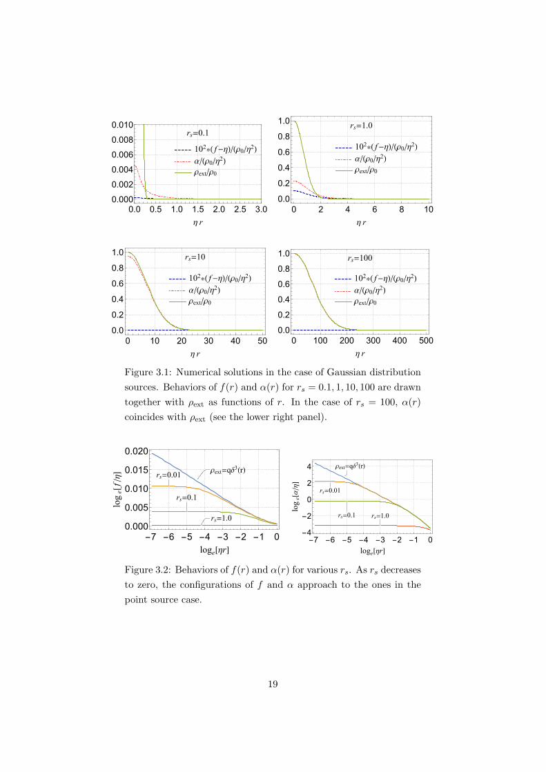
We depict the induced charge density ρind(r) with the external charge den-
sity ρext(r) in Fig.3.3. The sign of ρind is opposite to ρext. In the central
region of rs = 0.1 and rs = 1 cases, we find that |ρext| is larger than |ρind|,i.e., total charge density ρtotal(r) has the same sign with ρext(r). As r in-
creases, |ρind| exceeds |ρext|. In the region r ≫ rA, the both ρext and ρind
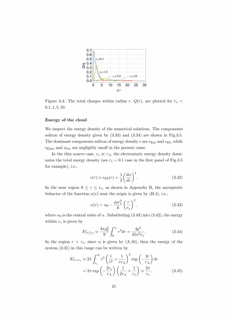
decrease quickly to zero. As shown in Fig.3.4, Q(r), the total charge within
radius r, decreases to zero in the region r ≫ max(rA, rs), it means the ex-
ternal charge is totally screened by the induced charge cloud for a distant
observer.
ρext/ρ0ρind/ρ0ρtotal/ρ0
0.0 0.5 1.0 1.5 2.0 2.5 3.0-0.004-0.0020.0000.0020.0040.0060.0080.010
η r
rs=0.1 ρext/ρ0ρind/ρ0ρtotal/ρ0
0 2 4 6 8 10-0.2
0.0
0.2
0.4
0.6
0.8
1.0
η r
rs=1.0
ρext/ρ0ρind/ρ0ρtotal/ρ0
0 10 20 30 40 50-1.0
-0.5
0.0
0.5
1.0
η r
rs=10 ρext/ρ0ρind/ρ0ρtotal/ρ0
0 100 200 300 400 500-1.0
-0.5
0.0
0.5
1.0
η r
rs=100
Figure 3.3: The external charge density, ρext(r), the induced charge
density, ρind(r), and sum of them, ρtotal(r), are plotted as functions
of r for rs = 0.1, 1, 10, 100.
In the case of rs ≪ rA, the width of the induced charge cloud is the
order of rA, while in the case of rs ≥ rA, the width is almost same as rs. In
the case of rs = 100, we have
ρind(r) = −ρext(r), (3.41)
as is justified by (B.7). Then, ρtotal vanishes everywhere, equivalently Q(r)
vanishes everywhere. We call this ‘perfect screening’.
20
rs=0.1
rs=1.0rs=5.0 rs=10
0 5 10 15 20 25 300.00.10.20.30.40.50.60.7
η r
Q/q
Figure 3.4: The total charges within radius r, Q(r), are plotted for rs =
0.1, 1, 5, 10.
Energy of the cloud
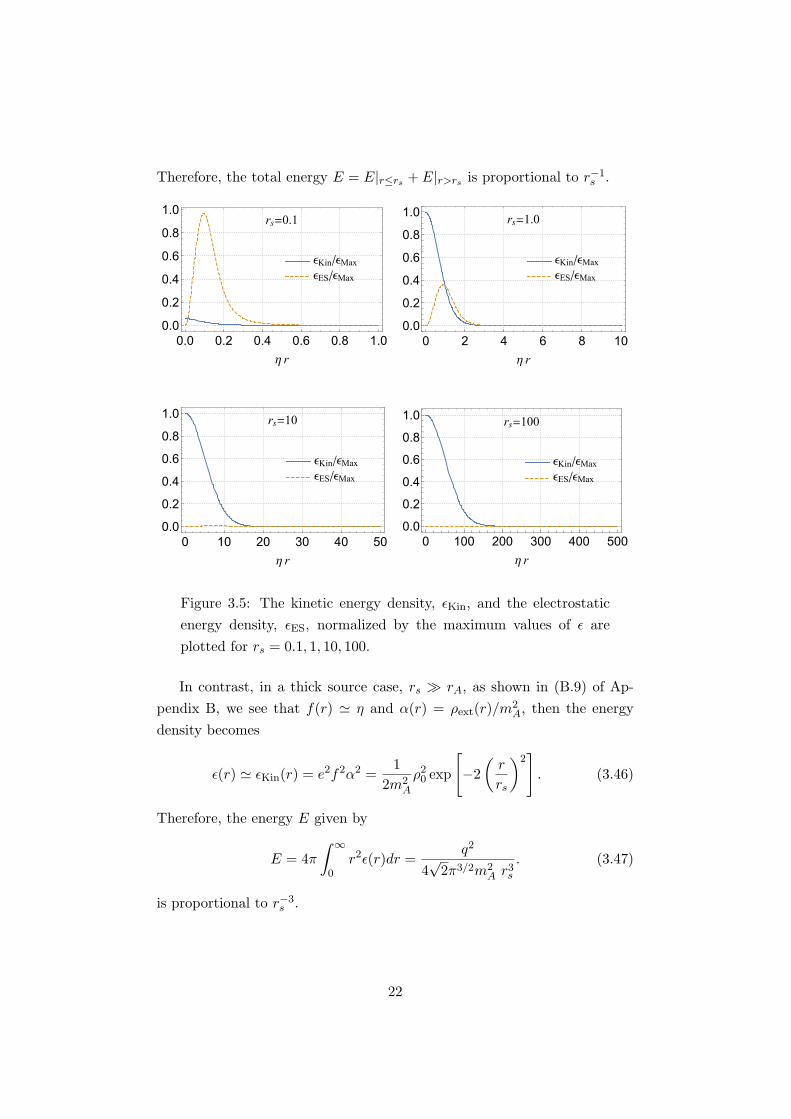
We inspect the energy density of the numerical solutions. The components
soliton of energy density given by (3.33) and (3.34) are shown in Fig.3.5.
The dominant components soliton of energy density ϵ are ϵKin and ϵES, while
ϵElast and ϵPot are negligibly small in the present cases.
In the thin source case, rs ≪ rA, the electrostatic energy density domi-
nates the total energy density (see rs = 0.1 case in the first panel of Fig.3.5
for example), i.e.,
ϵ(r) ≃ ϵES(r) =1
2
(dα
dr
)2
. (3.42)
In the near region 0 ≤ r ≤ rs, as shown in Appendix B, the asymptotic
behavior of the function α(r) near the origin is given by (B.4), i.e.,
α(r) ∼ α0 −ρ0r
2s
6
(r
rs
)2
, (3.43)
where α0 is the central value of α. Substituting (3.43) into (3.42), the energy
within rs is given by
E|r≤rs ≃4πρ209
∫ rs
0r4dr =
4q2
45π2rs. (3.44)
In the region r > rs, since α is given by (A.16), then the energy of the
system (3.31) in this range can be written by
E|r>rs ≃ 2π
∫ ∞
rs
r2(
1
r2+
1
rrA
)2
exp
(− 2r
rA
)dr
= 2π exp
(−2rsrA
)(1
2rA+
1
rs
)≃ 2π
rs. (3.45)
21
Therefore, the total energy E = E|r≤rs + E|r>rs is proportional to r−1s .
ϵKin/ϵMaxϵES/ϵMax
0.0 0.2 0.4 0.6 0.8 1.00.0
0.2
0.4
0.6
0.8
1.0
η r
rs=0.1
ϵKin/ϵMaxϵES/ϵMax
0 2 4 6 8 100.0
0.2
0.4
0.6
0.8
1.0
η r
rs=1.0
ϵKin/ϵMaxϵES/ϵMax
0 10 20 30 40 500.0
0.2
0.4
0.6
0.8
1.0
η r
rs=10
ϵKin/ϵMaxϵES/ϵMax
0 100 200 300 400 5000.0
0.2
0.4
0.6
0.8
1.0
η r
rs=100
Figure 3.5: The kinetic energy density, ϵKin, and the electrostatic
energy density, ϵES, normalized by the maximum values of ϵ are
plotted for rs = 0.1, 1, 10, 100.
In contrast, in a thick source case, rs ≫ rA, as shown in (B.9) of Ap-
pendix B, we see that f(r) ≃ η and α(r) = ρext(r)/m2A, then the energy
density becomes
ϵ(r) ≃ ϵKin(r) = e2f2α2 =1
2m2A
ρ20 exp
[−2
(r
rs
)2]. (3.46)
Therefore, the energy E given by
E = 4π
∫ ∞
0r2ϵ(r)dr =
q2
4√2π3/2m2
A r3s. (3.47)
is proportional to r−3s .
22
-2 -1 0 1 2
-6
-4
-2
0
log10[η rs]
log 10[E/η3 ]
rϕ=1.0 , rA=1.0
-2 -1 0 1 2
-6
-4
-2
0
log10[η rs]
log 10[E/η3 ]
rϕ=10 , rA=1.0
-2 -1 0 1 2 3
-8
-6
-4
-2
0
log10[η rs]
log 10[E/η3 ]
rϕ=1.0 , rA=10
-2 -1 0 1 2 3
-8
-6
-4
-2
0
log10[η rs]
log 10[E/η3 ]
rϕ=10 , rA=10
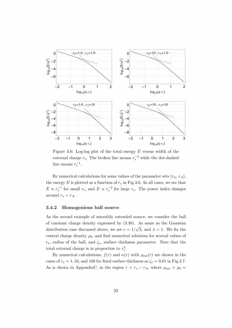
Figure 3.6: Log-log plot of the total energy E versus width of the
external charge rs. The broken line means r−3s while the dot-dashed
line means r−1s .
By numerical calculations for some values of the parameter sets (rϕ, rA),
the energy E is plotted as a function of rs in Fig.3.6. In all cases, we see that
E ∝ r−1s for small rs, and E ∝ r−3
s for large rs. The power index changes
around rs = rA.
3.4.2 Homogenious ball source
As the second example of smoothly extended source, we consider the ball
of constant charge density expressed by (3.38). As same as the Gaussian
distribution case discussed above, we set e = 1/√2, and λ = 1. We fix the
central charge density ρ0, and find numerical solutions for several values of
rs, radius of the ball, and ζs, surface thickness parameter. Note that the
total external charge is in proportion to r3s .
By numerical calculations, f(r) and α(r) with ρext(r) are shown in the
cases of rs = 1, 10, and 100 for fixed surface thickness as ζs = 0.01 in Fig.3.7.
As is shown in AppendixC, in the region r < rs − rA, where ρext ≃ ρ0 =
23
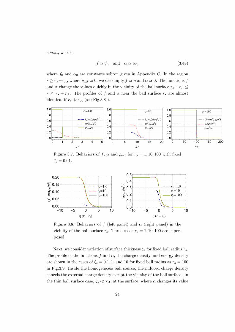
const., we see
f ≃ f0 and α ≃ α0, (3.48)
where f0 and α0 are constants soliton given in Appendix C. In the region
r ≥ rs+rA, where ρext ≃ 0, we see simply f ≃ η and α ≃ 0. The functions f
and α change the values quickly in the vicinity of the ball surface rs− rA ≤r ≤ rs + rA. The profiles of f and α near the ball surface rs are almost
identical if rs ≫ rA (see Fig.3.8 ).
( f-η)/(ρ0/η2)
α/(ρ0/η2)
ρext/ρ0
0 1 2 3 4 50.0
0.2
0.4
0.6
0.8
1.0
η r
rs=1.0
( f-η)/(ρ0/η2)
α/(ρ0/η2)
ρext/ρ0
0 5 10 15 200.0
0.2
0.4
0.6
0.8
1.0
η r
rs=10
( f-η)/(ρ0/η2)
α/(ρ0/η2)
ρext/ρ0
0 50 100 150 2000.0
0.2
0.4
0.6
0.8
1.0
η r
rs=100
Figure 3.7: Behaviors of f , α and ρext for rs = 1, 10, 100 with fixed
ζs = 0.01.
rs=1.0rs=10rs=100
-10 -5 0 5 100.00
0.05
0.10
0.15
0.20
η (r - rs)
(f-
η)/(ρ0/η2 )
rs=1.0rs=10rs=100
-10 -5 0 5 100.0
0.1
0.2
0.3
0.4
0.5
η (r - rs)
α/(ρ0/η2 )
Figure 3.8: Behaviors of f (left panel) and α (right panel) in the
vicinity of the ball surface rs. Three cases rs = 1, 10, 100 are super-
posed.
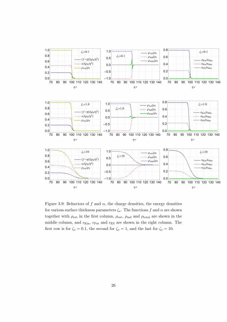
Next, we consider variation of surface thickness ζs for fixed ball radius rs.
The profile of the functions f and α, the charge density, and energy density
are shown in the cases of ζs = 0.1, 1, and 10 for fixed ball radius as rs = 100
in Fig.3.9. Inside the homogeneous ball source, the induced charge density
cancels the external charge density except the vicinity of the ball surface. In
the thin ball surface case, ζs ≪ rA, at the surface, where α changes its value
24
quickly, the induced charge exceeds the external charge inside the surface,
and vice versa outside. Therefore, an electric double layer emerges at the
surface of the ball. For the thick surface case, ζs ≫ rA, charge cancellation
occur everywhere even at the surface. Namely, the perfect screening occurs
in this case.
The components soliton of energy density given in (3.33) and (3.34) are
shown in Fig.3.9. Inside the homogeneous ball, the kinetic energy dominate
the energy density and the electrostatic energy density caused by the electric
double layer appears at the neighborhood of surface for the thin surface case.
25
( f-η)/(ρ0/η2)
α/(ρ0/η2)
ρext/ρ0
70 80 90 100 110 120 130 1400.0
0.2
0.4
0.6
0.8
1.0
η r
ζs=0.1 ρext/ρ0ρind/ρ0ρtotal/ρ0
70 80 90 100 110 120 130 140-1.0
-0.5
0.0
0.5
1.0
η r
ζs=0.1ϵKin/ϵMaxϵPot/ϵMaxϵES/ϵMax
70 80 90 100 110 120 130 1400.0
0.2
0.4
0.6
0.8
η r
ζs=0.1
( f-η)/(ρ0/η2)
α/(ρ0/η2)
ρext/ρ0
70 80 90 100 110 120 130 1400.0
0.2
0.4
0.6
0.8
1.0
η r
ζs=1.0 ρext/ρ0ρind/ρ0ρtotal/ρ0
70 80 90 100 110 120 130 140-1.0
-0.5
0.0
0.5
1.0
η r
ζs=1.0ϵKin/ϵMaxϵPot/ϵMaxϵES/ϵMax
70 80 90 100 110 120 130 1400.0
0.2
0.4
0.6
0.8
η r
ζs=1.0
( f-η)/(ρ0/η2)
α/(ρ0/η2)
ρext/ρ0
70 80 90 100 110 120 130 1400.0
0.2
0.4
0.6
0.8
1.0
η r
ζs=10 ρext/ρ0ρind/ρ0ρtotal/ρ0
70 80 90 100 110 120 130 140-1.0
-0.5
0.0
0.5
1.0
η r
ζs=10ϵKin/ϵMaxϵPot/ϵMaxϵES/ϵMax
70 80 90 100 110 120 130 1400.0
0.2
0.4
0.6
0.8
η r
ζs=10
Figure 3.9: Behaviors of f and α, the charge densities, the energy densities
for various surface thickness parameters ζs. The functions f and α are shown
together with ρext in the first column, ρext, ρind and ρtotal are shown in the
middle column, and ϵKin, ϵPot and ϵES are shown in the right column. The
first row is for ζs = 0.1, the second for ζs = 1, and the last for ζs = 10.
26
Chapter 4
Q-balls in a Spontaneously
Broken U(1) Gauge Theory
In the previous charpter, we investigated the total charge screening of an
external souorce in a spontaneously broken U(1) gauge theory. As a result,
we found that an arbitrary localized source is always totally screened by the
charge density of the complex Higgs scalar field coupled with a U(1) gauge
field.
In this chapter, we construct a Q-ball solution by introducing another
complex matter scalar field instead of the external source. We show that
the total charge screening occurs for the Q-balls.
4.1 Q-balls and gauged Q-balls in a coupled two
scalar fields model
Spherically symmetric nontopological solitons, i.e., Q-balls are first proposed
by R. Friedberg, T.D. Lee, and A. Sirlin [6]. They assumed a system consisits
of a real scalar field with a potential and a complex matter scalar field given
by
S =
∫d4x
(−(∂µψ)
∗(∂µψ)− 1
2(∂µϕ)(∂
µϕ)− λ
4(ϕ2 − η2)2 − µψ∗ψϕ2
),
(4.1)
where the firld ϕ breaks Z2 symmetry spontaneously. In 1991 X. Shi and
X.Z. Li generalized the Q-balls by assuming a local U(1) gauge invariance
27
[21]. The action is given by
S =
∫d4x
(−(Dµψ)
∗(Dµψ)− 1
2(∂µϕ)(∂
µϕ)− λ
4(ϕ2 − η2)2 − µψ∗ψϕ2 − 1
4FµνF
µν
).
(4.2)
In the sysytem, since the U(1) gauge field is coupled only with the matter
scalar field, charge screening can not occur. We replace a real scalar field to
a complex Higgs scalar field.
4.2 Basic Model
We consider the action given by
S =
∫d4x
(−(Dµψ)
∗(Dµψ)− (Dµϕ)∗(Dµϕ)− V (ϕ)− µψ∗ψϕ∗ϕ− 1
4FµνF
µν
),
(4.3)
where ψ is a complex matter scalar field, ϕ is a complex Higgs scalar field
with the potential
V (ϕ) :=λ
4(ϕ∗ϕ− η2)2, (4.4)
where λ and η are positive constants, and Fµν := ∂µAν − ∂νAµ is the field
strength of a U(1) gauge field Aµ. The covariant derivative Dµ in (4.3) is
defined by
Dµψ := ∂µψ − ieAµψ, Dµϕ := ∂µϕ− ieAµϕ, (4.5)
where e is a gauge coupling constant. This model is a generalization of the
Friedberg-Lee-Sirlin model by introducing a complex Higgs scalar field and
a U(1) gauge field.
The action (4.3) is invariant under the local U(1) times the global U(1)
gauge transformations,
ψ(x) → ψ′(x) = ei(χ(x)−γ)ψ(x), (4.6)
ϕ(x) → ϕ′(x) = ei(χ(x)+γ)ϕ(x), (4.7)
Aµ(x) → A′µ(x) = Aµ(x) + e−1∂µχ(x), (4.8)
where χ(x) and γ are an arbitrary function and a constant, respectively.
Owing to the gauge invariance, there are the conserved current
jνψ := ie ψ∗(Dνψ)− ψ(Dνψ)∗ , (4.9)
jνϕ := ie ϕ∗(Dνϕ)− ϕ(Dνϕ)∗ (4.10)
28
satisfying ∂µjµψ=0 and ∂µj
µϕ=0. Consequently, the total charge of ψ and ϕ
defined by
Qψ :=
∫ρψd
3x, (4.11)
Qϕ :=
∫ρϕd
3x, (4.12)
are conserved, where ρψ := jtψ and ρϕ := jtϕ.
The energy of the system is given by1
E =
∫d3x
(|Dtψ|2 + (Diψ)
∗(Diψ) + |Dtϕ|2 + (Diϕ)∗(Diϕ)
+ V (ϕ) + µ|ψ|2|ϕ|2 + 1
2
(EiE
i +BiBi))
, (4.13)
where Ei := Fi0, Bi := 1/2ϵijkFjk, and i denotes a spatial index. In the
vacuum state, which minimizes the energy (4.13), the fields ψ, ϕ, and Aµ
should satisfy
ψ = 0, ϕ∗ϕ = η2, Dµϕ = 0, and Fµν = 0, (4.14)
equivalently,
ψ = 0, ϕ = ηeiθ(x), and Aµ = e−1∂µθ, (4.15)
where θ is an arbitrary continuous regular function. We exclude topologi-
cally non-trivial case in this paper. The Higgs scalar field ϕ has the vacuum
expectation value η, then the Ulocal(1)×Uglobal(1) symmetry is broken into
a global U(1) symmetry, so that the gauge field Aµ and the complex scalar
field ψ acquire the mass mA =√2eη and mψ =
√µη, respectively. The
real scalar field that denotes a fluctuation of the amplitude of ϕ around η
acquires the mass mϕ =√λη.
By varying (4.3) with respect to ψ∗, ϕ∗, and Aµ, we obtain the equations
of motion
DµDµψ − µϕ∗ϕψ = 0, (4.16)
DµDµϕ− λ
2ϕ(ϕ∗ϕ− η2)− µϕψ∗ψ = 0, (4.17)
∂µFµν = jνϕ + jνψ. (4.18)
1See Appendix D.
29
We assume that the fields are stationary and spherically symmetric in
the form,
ψ = eiωtu(r), (4.19)
ϕ = eiω′tf(r), (4.20)
At = At(r), and Ai = 0, (4.21)
where ω and ω′ are constants, u(r) and f(r) are real functions of r. Using
the gauge transformation (4.6), (4.7) and (4.8), we fix the variables as
ϕ(r) → f(r), (4.22)
ψ(t, r) → eiΩtu(r) := ei(ω−ω′)tu(r), (4.23)
At(r) → α(r) := At(r)− e−1ω′, (4.24)
where we assume Ω := ω − ω′ > 0 without loss of generality.
Substituting (4.22), (4.23), and (4.24) into (4.16), (4.17), and (4.18), we
obtain a set of the ordinary differential equations:
d2u
dr2+
2
r
du
dr+ (eα− Ω)2u− µf2u = 0, (4.25)
d2f
dr2+
2
r
df
dr+ e2fα2 − λ
2f(f2 − η2)− µfu2 = 0, (4.26)
d2α
dr2+
2
r
dα
dr+ ρtotal = 0, (4.27)
where ρtotal is defined by
ρtotal(r) := ρψ(r) + ρϕ(r). (4.28)
The charge densities ρψ and ρϕ are given by the variables u, f , and α as
ρψ = −2e(eα− Ω)u2, (4.29)
ρϕ = −2e2αf2. (4.30)
We seek configurations of the fields with a non-vanishing value of Ω that
characterizes the solutions.
We require boundary conditions for the fields so that the fields should
be regular at the origin. Then, we impose the conditions for the spherically
symmetric fields as
du
dr→ 0 ,
df
dr→ 0 ,
dα
dr→ 0 as r → 0. (4.31)
30
On the other hand, fields should be in the vacuum state at the spatial
infinity. Therefore, from (3.18) we impose the conditions
u→ 0 , f → η , α→ 0 as r → ∞. (4.32)
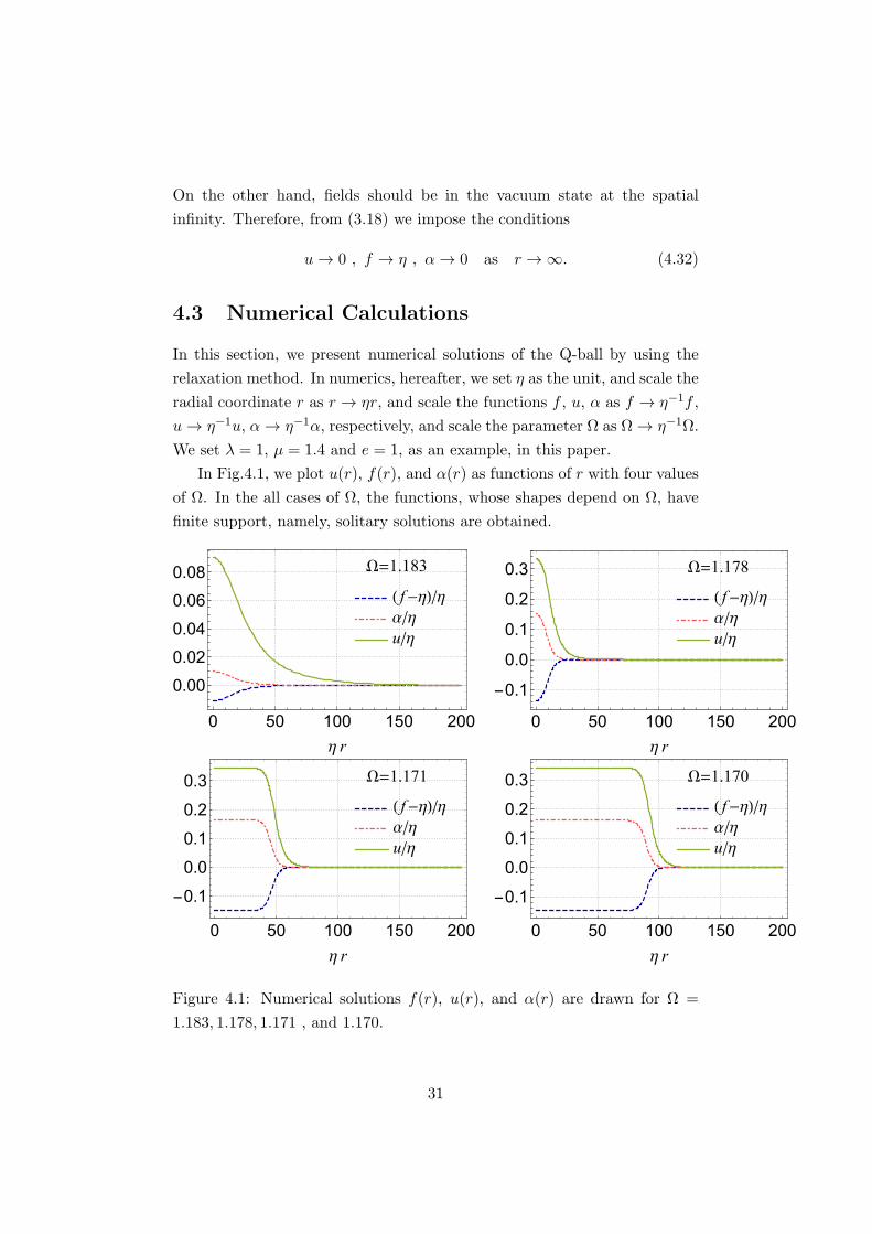
4.3 Numerical Calculations
In this section, we present numerical solutions of the Q-ball by using the
relaxation method. In numerics, hereafter, we set η as the unit, and scale the
radial coordinate r as r → ηr, and scale the functions f , u, α as f → η−1f ,
u→ η−1u, α→ η−1α, respectively, and scale the parameter Ω as Ω → η−1Ω.
We set λ = 1, µ = 1.4 and e = 1, as an example, in this paper.
In Fig.4.1, we plot u(r), f(r), and α(r) as functions of r with four values
of Ω. In the all cases of Ω, the functions, whose shapes depend on Ω, have
finite support, namely, solitary solutions are obtained.
( f-η)/η
α/η
u/η
0 50 100 150 200
0.00
0.02
0.04
0.06
0.08
η r
Ω=1.183
( f-η)/η
α/η
u/η
0 50 100 150 200
-0.1
0.0
0.1
0.2
0.3
η r
Ω=1.178
( f-η)/η
α/η
u/η
0 50 100 150 200
-0.1
0.0
0.1
0.2
0.3
η r
Ω=1.171
( f-η)/η
α/η
u/η
0 50 100 150 200
-0.1
0.0
0.1
0.2
0.3
η r
Ω=1.170
Figure 4.1: Numerical solutions f(r), u(r), and α(r) are drawn for Ω =
1.183, 1.178, 1.171 , and 1.170.
31
In the case of Ω = 1.183 and Ω = 1.178, the field profiles are Gaussian
function like. On the other hand, for Ω = 1.171, Ω = 1.170, the field
profiles are step function like. The solutions in the latter cases represent
homogeneous balls, namely, the functions u, f and α take constant values
inside the ball, and they change the values quickly in a thin region of the
ball surface, r = rs, and u, α vanish and f takes the vacuum expectation
value η outside the ball.
ρψ/ρψ(0)ρϕ/ρψ(0)ρtotal/ρψ(0)
0 50 100 150 200-1.0
-0.5
0.0
0.5
1.0
η r
Ω=1.183
ρψ/ρψ(0)ρϕ/ρψ(0)ρtotal/ρψ(0)
0 50 100 150 200-1.0
-0.5
0.0
0.5
1.0
η r
Ω=1.178
ρψ/ρψ(0)ρϕ/ρψ(0)ρtotal/ρψ(0)
0 50 100 150 200-1.0
-0.5
0.0
0.5
1.0
η r
Ω=1.171
ρψ/ρψ(0)ρϕ/ρψ(0)ρtotal/ρψ(0)
0 50 100 150 200-1.0
-0.5
0.0
0.5
1.0
η r
Ω=1.170
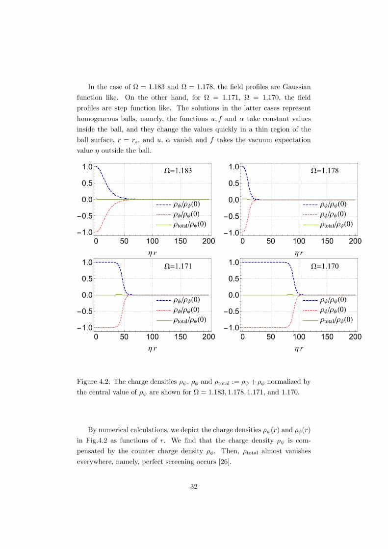
Figure 4.2: The charge densities ρψ, ρϕ and ρtotal := ρψ + ρϕ normalized by
the central value of ρψ are shown for Ω = 1.183, 1.178, 1.171, and 1.170.
By numerical calculations, we depict the charge densities ρψ(r) and ρϕ(r)
in Fig.4.2 as functions of r. We find that the charge density ρψ is com-
pensated by the counter charge density ρϕ. Then, ρtotal almost vanishes
everywhere, namely, perfect screening occurs [26].
32
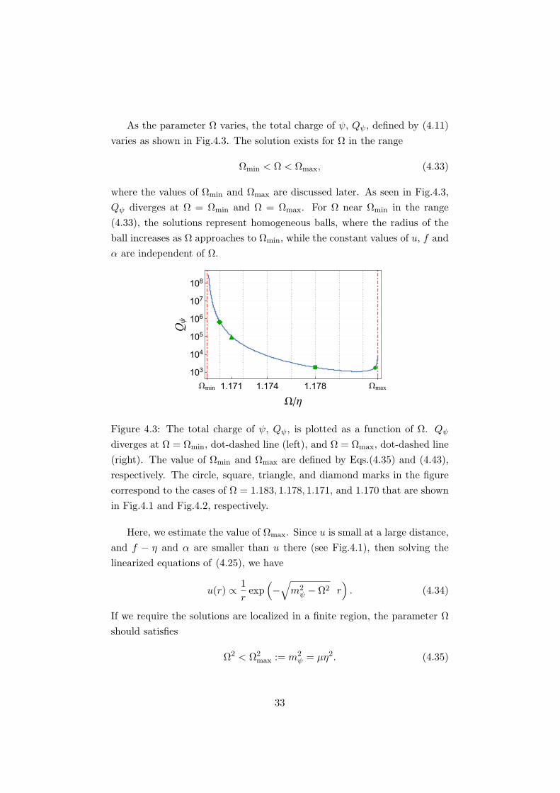
As the parameter Ω varies, the total charge of ψ, Qψ, defined by (4.11)
varies as shown in Fig.4.3. The solution exists for Ω in the range
Ωmin < Ω < Ωmax, (4.33)
where the values of Ωmin and Ωmax are discussed later. As seen in Fig.4.3,
Qψ diverges at Ω = Ωmin and Ω = Ωmax. For Ω near Ωmin in the range
(4.33), the solutions represent homogeneous balls, where the radius of the
ball increases as Ω approaches to Ωmin, while the constant values of u, f and
α are independent of Ω.
Ωmin 1.171 1.174 1.178 Ωmax
103
104
105
106
107
108
Ω/η
Qψ
Figure 4.3: The total charge of ψ, Qψ, is plotted as a function of Ω. Qψ
diverges at Ω = Ωmin, dot-dashed line (left), and Ω = Ωmax, dot-dashed line
(right). The value of Ωmin and Ωmax are defined by Eqs.(4.35) and (4.43),
respectively. The circle, square, triangle, and diamond marks in the figure
correspond to the cases of Ω = 1.183, 1.178, 1.171, and 1.170 that are shown
in Fig.4.1 and Fig.4.2, respectively.
Here, we estimate the value of Ωmax. Since u is small at a large distance,
and f − η and α are smaller than u there (see Fig.4.1), then solving the
linearized equations of (4.25), we have
u(r) ∝ 1
rexp
(−√m2ψ − Ω2 r
). (4.34)
If we require the solutions are localized in a finite region, the parameter Ω
should satisfies
Ω2 < Ω2max := m2
ψ = µη2. (4.35)
33
4.4 Homogeneous ball solutions
For the parameter Ω very closed to Ωmin, the homogeneous ball solutions
with large radius appear. We inspect the homogeneous ball solutions in
detail.
The set of equations (4.25), (4.26), and (4.27) can be derived from the
effective action in the form
Seff =
∫r2dr
((du
dr
)2
+
(df
dr
)2
− 1
2
(dα
dr
)2
− Ueff(u, f, α)
), (4.36)
Ueff(u, f, α) := −λ4(f2 − η2)2 − µf2u2 + e2f2α2 + (eα− Ω)2u2. (4.37)
If we regard the coordinate r as a ‘time’, the effective action (4.36) describes
a mechanical system of three degrees of freedom, u, f and α, where the
‘kinetic’ term of α has the wrong sign. In the case of the homogeneous ball
solution with a large radius, the damping terms that proportional to 1/r in
(4.25), (4.26), and (4.27) are negligible. In this case,
Eeff :=
(du
dr
)2
+
(df
dr
)2
− 1
2
(dα
dr
)2
+ Ueff(u, f, α) (4.38)
is conserved during the motion in the fictitious time r.
There are stationary points of the dynamical system on which
∂Ueff
∂u= 0,
∂Ueff
∂f= 0, and
∂Ueff
∂α= 0 (4.39)
are satisfied. Two stationary points exist in the region u ≥ 0, f ≥ 0, and
α ≥ 0. One stationary point, say Pv, exists at (u, f, α) = (0, η, 0), that is
the true vacuum. The other stationary point, say P0, exists at (u, f, α) =
(u0, f0, α0), where u0, f0, and α0 are given by solving (4.39) as
α0 =1
e(4µ− λ)
((µ− λ)Ω +
√µ(2λ+ µ)Ω2 − µλ(4µ− λ)η2
),
f0 =1√µ(Ω− eα0),
u0 =1õ
√eα0(Ω− eα0).
(4.40)
We note that 0 < eα0 < Ω should hold for real value of u0. This condition
with (4.35) requires
λ < µ. (4.41)
34
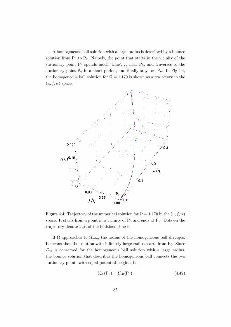
A homogeneous ball solution with a large radius is described by a bounce
solution from P0 to Pv. Namely, the point that starts in the vicinity of the
stationary point P0 spends much ‘time’, r, near P0, and traverses to the
stationary point Pv in a short period, and finally stays on Pv. In Fig.4.4,
the homogeneous ball solution for Ω = 1.170 is shown as a trajectory in the
(u, f, α) space.
Figure 4.4: Trajectory of the numerical solution for Ω = 1.170 in the (u, f, α)
space. It starts from a point in a vicinity of P0 and ends at Pv. Dots on the
trajectory denote laps of the fictitious time r.
If Ω approaches to Ωmin, the radius of the homogeneous ball diverges.
It means that the solution with infinitely large radius starts from P0. Since
Eeff is conserved for the homogeneous ball solution with a large radius,
the bounce solution that describes the homogeneous ball connects the two
stationary points with equal potential heights, i.e.,
Ueff(Pv) = Ueff(P0). (4.42)
35
We see that this occurs for
Ω = Ωmin :=
√2√λµ− λ η =
√mϕ(2mψ −mϕ). (4.43)
Then, for the parameters satisfying (4.41), we see
Ωmin < Ωmax. (4.44)
Then, the non-topological soliton solutions exist for the model parameters
with (4.41).
We can estimate the value of Ωmax and Ωmin given by (4.35) and (4.43)
using the parameters λ, µ, and η in the numerical calculations as Ωmax ∼1.1832 and Ωmin ∼ 1.1689. We see in Fig.4.3 that numerical calculation
reproduce these values.
Using the ansatz (4.22), (4.23), and (4.24), we rewrite the energy (3.17)
for the symmetric system as
ENTS = 4π
∫ ∞
0r2ϵ(r)dr, (4.45)
ϵ := ϵψKin + ϵϕKin + ϵψElast + ϵϕElast + ϵInt + ϵPot + ϵES, (4.46)
where
ϵψKin := |Dtψ|2 = (eα− Ω)2u2, ϵϕKin := |Dtϕ|2 = e2f2α2,
ϵψElast := (Diψ)∗(Diψ) =
(du
dr
)2
, ϵϕElast := (Diϕ)∗(Diϕ) =
(df
dr
)2
,
ϵPot := V (ϕ) =λ
4(f2 − η)2, ϵInt := µ|ϕ|2|ψ|2 = µf2u2, ϵES :=
1
2EiE
i =1
2
(dα
dr
)2
,
(4.47)
are densities of kinetic energy of ψ and ϕ, elastic energy of ψ and ϕ, po-
tential energy of ϕ, interaction energy between ψ and ϕ, and electrostatic
energy, respectively. For the homogeneous ball solutions, these components
of energy density are shown in Fig.4.5. The dominant components of the
energy density ϵ are ϵψKin and ϵInt, and subdominant components are ϵϕKin
and ϵPot for the present cases. The densities of the elastic energy and the
electrostatic energy, which appear near the surface of the ball, are negligibly
small, then, they are not plotted.
36
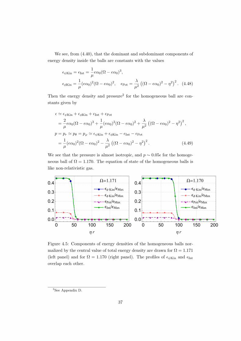
We see, from (4.40), that the dominant and subdominant components of
energy density inside the balls are constants with the values
ϵψKin = ϵInt =1
µeα0(Ω− eα0)
3,
ϵϕKin =1
µ(eα0)
2(Ω− eα0)2, ϵPot =
λ
µ2((Ω− eα0)
2 − η2)2. (4.48)
Then the energy density and pressure2 for the homogeneous ball are con-
stants given by
ϵ ≃ ϵψKin + ϵϕKin + ϵInt + ϵPot
=2
µeα0(Ω− eα0)
3 +1
µ(eα0)
2(Ω− eα0)2 +
λ
µ2((Ω− eα0)
2 − η2)2,
p = pr ≃ pθ = pφ ≃ ϵψKin + ϵϕKin − ϵInt − ϵPot
=1
µ(eα0)
2(Ω− eα0)2 − λ
µ2((Ω− eα0)
2 − η2)2. (4.49)
We see that the pressure is almost isotropic, and p ∼ 0.05ϵ for the homoge-
neous ball of Ω = 1.170. The equation of state of the homogeneous balls is
like non-relativistic gas.
ϵψKin/ϵMax
ϵϕKin/ϵMax
ϵPot/ϵMax ϵInt/ϵMax
0 50 100 150 2000.0
0.1
0.2
0.3
0.4
η r
Ω=1.171
ϵψKin/ϵMax
ϵϕKin/ϵMax
ϵPot/ϵMax ϵInt/ϵMax
0 50 100 150 2000.0
0.1
0.2
0.3
0.4
η r
Ω=1.170
Figure 4.5: Components of energy densities of the homogeneous balls nor-
malized by the central value of total energy density are drawn for Ω = 1.171
(left panel) and for Ω = 1.170 (right panel). The profiles of ϵψKin and ϵInt
overlap each other.
2See Appendix D.
37
In the limit Ω → Ωmin, so that Qψ → ∞, we see
ϵψKin = ϵInt →λ(√µ−
√λ)√µ
(2√µ−
√λ)2
η4,
ϵϕKin → λ
( √µ−
√λ
2√µ−
√λ
)2
η4, ϵPot → λ
( √µ−
√λ
2√µ−
√λ
)2
η4, (4.50)
then we have
ϵ→2λ(
√µ−
√λ)
2√µ−
√λ
η4,
p→ 0. (4.51)
Therefore, in the large homogeneous ball limit, the ball becomes dust ball
with constant energy density given by (4.51).
4.5 Stability
The nontopological soliton, called Q-ball, can be interpreted as a condensate
of particles of the scalar field ψ, where the Higgs field plays the role of glue
against repulsive force by the U(1) gauge field. We compare energy of the
soliton, ENTS, given by (4.45) with mass energy of the free particles of ψ
that have the same amount of charge of the soliton as a whole. Then, the
numbers of the particles is defined by
Nψ :=Qψe, (4.52)
and the mass energy of the free particles of ψ is given by Efree = mψNψ.
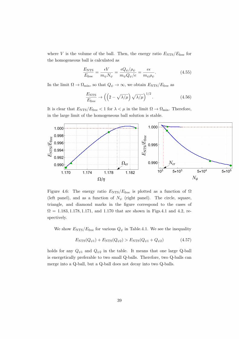
Fig.4.6 shows the energy ratio ENTS/Efree as a function of Ω and as a
function of Nψ, respectively. We find a critical value of Ω, Ωcr, such that if
Ω < Ωcr, ENTS < Efree holds. Therefore, a Q-ball for Ω in the range
Ωmin < Ω < Ωcr (4.53)
is energetically preferable than the free ψ particles with the same charge of
the Q-ball as a whole. From the Fig.4.6, there exist stable Q-balls that are
condensates of large numbers of ψ particles.
Since the energy density and charge density are constant inside the ball,
the total energy and the total charge of matter field of the homogeneous ball
are written by
ENTS = ϵV, and Qψ = ρψV, (4.54)
38
where V is the volume of the ball. Then, the energy ratio ENTS/Efree for
the homogeneous ball is calculated as
ENTS
Efree=
ϵV
mψNψ=
ϵQψ/ρψmψQψ/e
=eϵ
mψρψ. (4.55)
In the limit Ω → Ωmin, so that Qψ → ∞, we obtain ENTS/Efree as
ENTS
Efree→((
2−√λ/µ
)√λ/µ
)1/2. (4.56)
It is clear that ENTS/Efree < 1 for λ < µ in the limit Ω → Ωmin. Therefore,
in the large limit of the homogeneous ball solution is stable.
Ωcr
1.170 1.174 1.178 1.182
0.990
0.992
0.994
0.996
0.998
1.000
Ω/η
ENTS/Efree
Ncr
103 5*103 5*104 5*105
0.990
0.995
1.000
Nψ
ENTS/Efree
Figure 4.6: The energy ratio ENTS/Efree is plotted as a function of Ω
(left panel), and as a function of Nψ (right panel). The circle, square,
triangle, and diamond marks in the figure correspond to the cases of
Ω = 1.183, 1.178, 1.171, and 1.170 that are shown in Figs.4.1 and 4.2, re-
spectively.
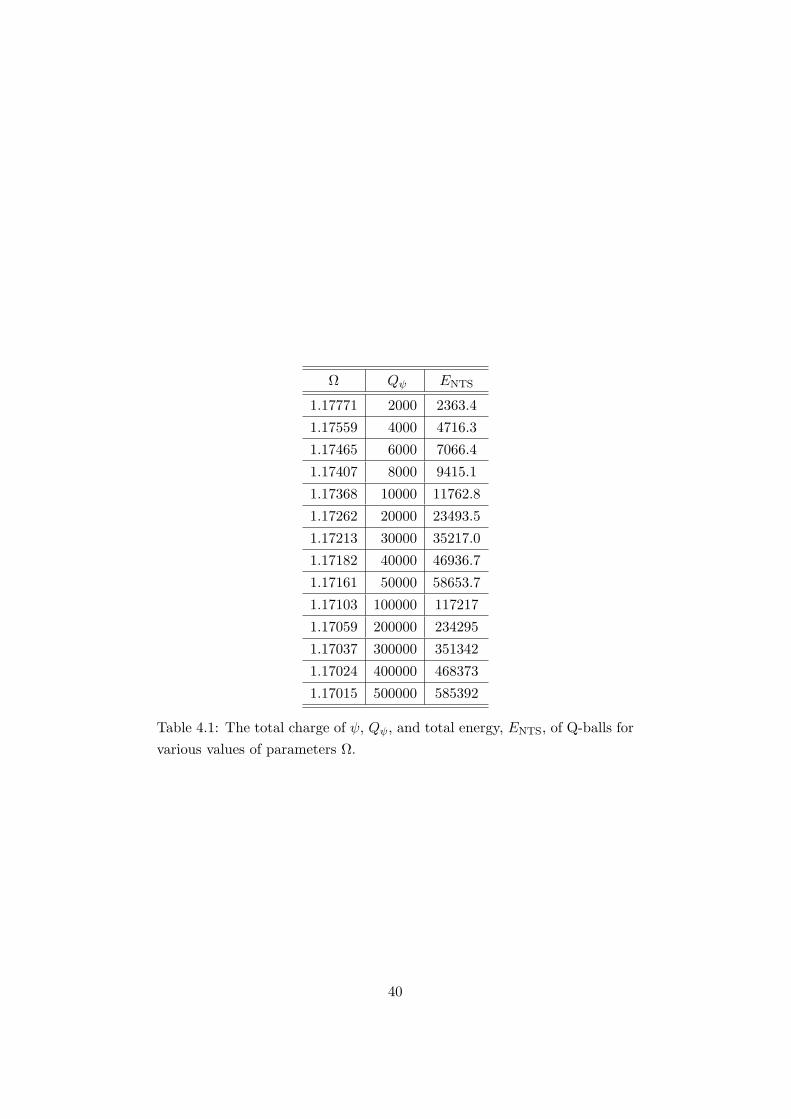
We show ENTS/Efree for various Qψ in Table.4.1. We see the inequality
ENTS(Qψ1) + ENTS(Qψ2) > ENTS(Qψ1 +Qψ2) (4.57)
holds for any Qψ1 and Qψ2 in the table. It means that one large Q-ball
is energetically preferable to two small Q-balls. Therefore, two Q-balls can
merge into a Q-ball, but a Q-ball does not decay into two Q-balls.
39
Ω Qψ ENTS
1.17771 2000 2363.4
1.17559 4000 4716.3
1.17465 6000 7066.4
1.17407 8000 9415.1
1.17368 10000 11762.8
1.17262 20000 23493.5
1.17213 30000 35217.0
1.17182 40000 46936.7
1.17161 50000 58653.7
1.17103 100000 117217
1.17059 200000 234295
1.17037 300000 351342
1.17024 400000 468373
1.17015 500000 585392
Table 4.1: The total charge of ψ, Qψ, and total energy, ENTS, of Q-balls for
various values of parameters Ω.
40
Chapter 5
Summary
In this paper, we studied the Q-ball solutions whose charge is totally screened
in a spontaneouly broken U(1) gauge theory. We first investigated the total
charge screening of an external source before constructing Q-balls.
In Chap.2, we introduced a scalar field theories with a U(1) symmetry.
We reviewed the standard idea, that is, by promoting the global U(1) sym-
metry to the local symmetry by introducing a gauge field, and it acquires a
mass through the Higgs mechanism.
In Chap.3, first, we showed the total charge screening by using a massive
vector field, i.e., Proca field always occurs. Based on the result of the Proca
field, we studied the classical system that consists of a U(1) gauge field and
a complex Higgs scalar field with a potential that causes the spontaneous
symmetry breaking. We presented numerical solutions in the presence of a
smoothly extended external source with a finite size. We have investigated
two kinds of extended external sources: Gaussian distribution sources and
homogeneous ball sources. In the case of Gaussian distribution source, the
profile of the total charge within radius r, Q(r), depends on the width of the
external source, rs. In the thin source case, where rs is much smaller than the
mass scale of the vector field, rA = m−1A , non-vanishing peak of Q(r) appears
at a radius in the range r < rs. Then, the charge density is detectable in the
region r < rs. The maximum value of Q(r) is less than the total external
charge, then the partial screening occurs in a finite distance. As r increases,
Q(r) damps quickly, then the total charge screening occurs by the induced
charge cloud for a distant observer. In the thick source case, where rs is much
larger than rA, Q(r) is almost zero everywhere, equivalently, ρtotal almost
vanishes everywhere. In this case, the charge is perfectly screened so that
41
the charge is not detectable anywhere. For the homogeneous ball source, we
have considered that the charge density is constant within the ball radius, rs,
which is assumed to be much larger than rA, and the charge density varies
with the surface thickness scale, ζs, at the ball surface. We found that inside
the ball, r < rs−rA, the amplitude of the scalar field and the gauge field take
constant values, respectively, and outside the ball, r > rs + rA, the scalar
field takes the vacuum expectation value and the gauge field vanishes. At
the ball surface, the both fields change their values quickly. The external
charge is canceled out by the induced charge cloud except the vicinity of ball
surface. In the thin surface case, ζs ≪ rA, electric double layer appears at
the ball surface. In the thick surface case, ζs ≫ rA, the charge cancellation
occurs even at the ball surface, namely, the perfect screening occurs. The
kinetic energy and the potential are main components of the energy density
inside the ball. For the thin surface case, the electrostatic component of the
energy density by the electric double layer appears at the ball surface.
In Chap.4, we studied the coupled system of a complex matter scalar
field, a U(1) gauge field, and a complex Higgs scalar field with a potential
that causes the spontaneous symmetry breaking. This is a generalization
of the Friedberg-Lee-Sirlin model [6]. In this model a global U(1) × Z2
symmetry is assumed. On the other hand, our system has a local U(1) ×global U(1) symmetry. Promotion of a global symmetry to a local one is a
natural extention in field theories. The local U(1)× global U(1) symmetry
in this system is broken spontaneously into a global U(1) symmetry by the
Higgs field. We have shown numerically that there are spherically symmetric
nontopological soliton solutions, Q-balls, that are characterized by phase
rotation of the complex matter scalar field, Ω. The solutions exist for Ω
in the range Ωmin < Ω < Ωmax. The lower bound, Ωmin, appears in order
to localiz the fields, and it is given by mass of the complex scalar matter
field as Ωmin = mψ. In the nontopological soliton solutions, charge densities
are induced by the matter scalar field and the Higgs field, respectively, and
they are totally screened each other. As a result, the Q-balls behave as
electrically neutral objects for distant observers.
If we assume the stationary and spharically symmetry, and if we regard
the radial coordinate as a “time” and the value of the fields as a position of
a particle, the system is analogous to a dynamical system of the particle in
three dimensions. The equations of motion for the fields are derived from an
42
effective action Seff which includes an effective potential Ueff. The system
has a friction that is in proportion to the inverse of “time”, i.e., r−1. If the
motion of the particle occurs in a range of large r, the frictional term can
be negligible, and the effective “energy” Eeff is conserved during the motion
in the fictitious “time”. The present dynamical system has some stationary
points. One of them corresponds to the vacuum. We found typical solutions
that the particle starts from a stationary point traverse toward the vac-
uum stationary point, we call them the bounce solutions. The trajectories
for the bounce solutions in three dimensional space connect two station-
ary points with the same potential height. We found stationary points for
the bounce solutions exist in the effective potential: one corresponds to the
true vacuum, say Pv, and the other is a nontrivial point, say P0. In the
limit Ω → Ωmin, values of the effective potential take same value at the two
stationary points respectively, U(Pv) = U(P0). Then radius of the Q-ball
diverges, and therefore, the charge and the mass diverge. We called the
bounce solutions homogeneous ball, namely, the fields takes constant val-
ues inside the ball. For the homogeneous balls, perfect screening occurs,
namely, the charge density of matter scalar field is canceled out everywhere
by the counter charge cloud of the Higgs and the gauge fields. Inspecting the
energy-momentum tensor of the fields, we showed that the pressure inside
the ball is almost isotropic, and the value is much less than the energy den-
sity. Then, a homogeneous ball is like a ball of homogeneous nonrelativistic
gas. Especially, in the limit Ω → Ωmin, the pressure vanishses and then the
ball behaves as dust with constant energy density.
The Q-balls obtained in this paper would have applications in cosmology
and astrophysics. The total screening of the charge is a preferable property
for the gauged Q-balls to be dark matter [12, 13, 14, 15, 16]. It is an impor-
tant issue how much amount of the Q-balls are produced in the evolution
of the universe [43, 44, 45, 46, 47, 48]. It would be an interesting problem
to clarify the mass distribution spectrum of the Q-balls, which would evolve
by merging process of Q-balls, in the present stage of the universe.
Furthermore, our planned future works are divided into three issues:
searching other types of the large Q-balls; investigating stability for the Q-
balls in our system; and taking the Einstein gravity into account. Large
Q-balls studied in this paper could be interpreted as bounce solutions from
one stationary point P0 to the vacuum stationary point Pv. In addition,
43
other types of the bounce solutions may be constructed since the effective
potential of the system admits other stationary points1. If other types of
the large Q-balls exist, they would behaves as other components compared
with them in this paper.
We investigated stability for the Q-balls energetically in this paper. This
is the simplest discussion for stability . However, it is not enough for proov-
ing stability of the Q-balls. An alternative analysis is the dynamical sta-
bility. This is achived by solving eigenvalue problems for perturbed field
equations. This is a very important issue in order to apply our Q-balls
to the cosmology and the astrophysics. There are various view points for
stability [30, 31, 32, 33, 34, 35].
We proved that the dust ball is energetically stable. Although the dust
balls have no limit of mass, if we take the gravity into account, arbitrary
large mass can not be allowed. If the mass of the dust ball becomes too
large so that the pressure fails to sustain the gravity, the ball would collapse
to a black hole. It is an interesting issue to study the gravitational effects
on the Q-balls [36, 37, 38, 39, 41]. In the case of the boson stars, upper
bound of mass exist for stability. It would be also an interesting problem
to clarify that these boson stars could be origins of primordial black holes
and/or super massive black holes in the central region of galaxies.
1We obtain other types of Q-ball solutions as shown in Appendix E.
44
Appendicies
Appendix A Charge Screning of a Point source
We analyze asymptotic behaviors of the scalar and gauge fields governed by
(3.29) and (3.30) for a point source, where the charge density is given by
the δ-function as
ρext(r) = qδ3(r), (A.1)
where q denotes the total external charge [57, 58]. The equations admit
an exact solution α(r) = q/(4πr) and f(r) = 0, the Coulomb solution.
However, this configuration does not minimize the energy (3.17), i.e., not
the vacuum. To seek other solutions with non-vanishing f(r), we discuss
asymptotic behavior of the fields near the point source and at infinity. We
set e = 1/√2 and λ = 1 so that rϕ := m−1
ϕ = 1 and rA := m−1A = 1.
A.1 Asymptotic behaviors for the point source
We assume that the asymptotic behavior of the fields in the vicinity of the
point source are given by
α(r) ∼ a1rγ , (A.2)
f(r) ∼ b1rβ. (A.3)
where a1 and b1 are non-vanishing constants. Substituting these expression
in (3.29) and (3.30), we obtain
β(β − 1)rβ−2 + 2βrβ−2 + e2a21rβ+2γ − λ
2b21r
3β +λ
2rβ = 0, (A.4)
γ(γ − 1)rγ−2 + 2γrγ−2 − 2e2b21r2β+γ = 0. (A.5)
45
First, we consider the case of β > −1. In this case, we can ignore the
third term in (A.5), and obtain γ = −1. By Gauss’ integral theorem applied
in a small volume including the point source, we have
α =a1r
=q
4πr. (A.6)
Since β > −1 and γ = −1, the first three terms in (A.4) should compensate
each other. Then, we obtain
β =1
2
(−1±
√1− 4κ2
)(A.7)
where κ := eq/4π.
If κ ≤ 1/2, β is real number. For the upper sign in (A.7), the elastic
energy density ϵEla defined in (3.33) is finite in the limit r → 0, however it
diverges for the lower sign. Then, we take the positive sign in (A.7) for the
power index of f .
If κ > 1/2, β becomes complex numbers
β =1
2
(−1± i
√4κ2 − 1
), (A.8)
then we have the real function f(r) in the form
f(r) =b1√rcos (σ log r + c1) , (A.9)
σ : =1
2
√4κ2 − 1, (A.10)
where b1 and c1 are constants soliton.
In the case of β ≤ −1, after some consideration, we see b1 should vanish.
Then, it is not the case in which the expected solution exists.
A.2 Distant region
At spatial infinity, α approaches to zero, and f does to η asymptotically.
Then, in the distant region, we rewrite f(r) as
f(r) ∼ η + δf(r), (A.11)
where δf → 0 as r → ∞. Substituting (A.11) to (3.29) and (3.30), we obtain
a set of linear differential equations
d2
dr2δf +
2
r
d
drδf − 1
r2ϕδf = 0, (A.12)
d2
dr2α+
2
r
d
drα− 1
r2Aα = 0, (A.13)
46
where higher order terms in δf and α are neglected. Solving these equations,
we obtain asymptotic behaviors of the functions as
δf(r) ∼ b2rexp
(− r
rϕ
), (A.14)
α(r) ∼ a2rexp
(− r
rA
), (A.15)
where b2 and a2 are constants soliton. These behaviors at the large distance
are general if the external source has a compact support around the origin.
A.3 Numerical calculations
As is shown in previous subsection, inspecting the equations (3.29) and
(3.30) near the origin, we obtain the asymptotic behavior of α in the form
of (A.6), and f is given by (A.3) for κ ≤ 1/2 or (A.9) for κ ≥ 1/2.
102*( f-η)/ηα/η
0 1 2 3 4 50
2
4
6
8
10
η r
κ=0.1
( f-η)/η
α/η
0 1 2 3 4 50
2
4
6
8
10
η r
κ=1.0
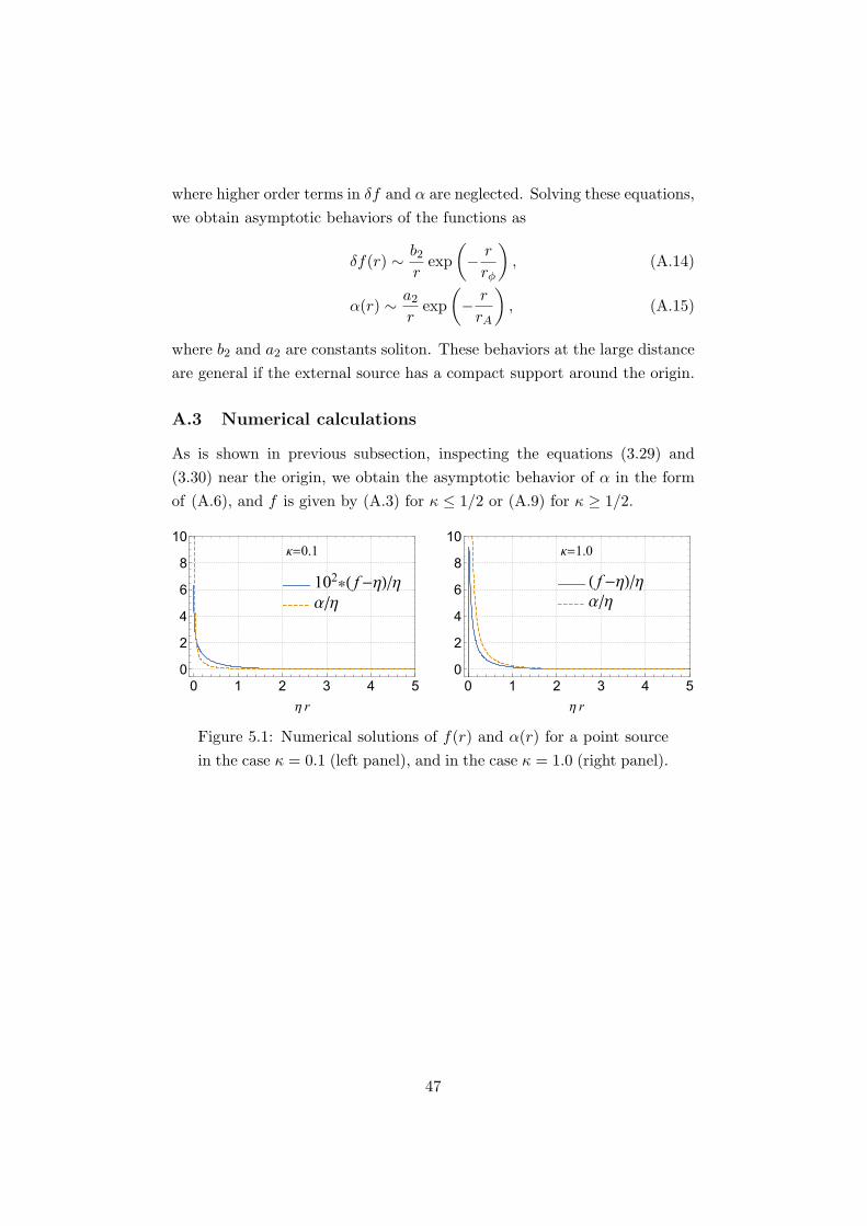
Figure 5.1: Numerical solutions of f(r) and α(r) for a point source
in the case κ = 0.1 (left panel), and in the case κ = 1.0 (right panel).
47
κ=0.1
κ=0.5
κ=0.2κ=0.3
κ=0.4
-7 -6 -5 -4 -3 -2 -1 0-0.50.00.51.01.52.02.53.0
log e[ηr]
loge[f/η]
κ=0.6κ=0.7
κ=0.8
κ=0.9
κ=1.0
-6 -5 -4 -3 -2 -1 0-1.5-1.0-0.50.00.51.01.5
loge[ηr]
log e[rf]
-6.5 -6.0 -5.5 -5.0
5.0
5.5
6.0
6.5
7.0
loge[ηr]
loge[α/η]
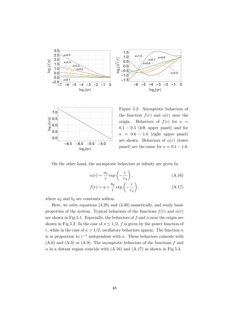
Figure 5.2: Asymptotic behaviors of
the function f(r) and α(r) near the
origin. Behaviors of f(r) for κ =
0.1 − 0.5 (left upper panel) and for
κ = 0.6 − 1.0 (right upper panel)
are shown. Behaviors of α(r) (lower
panel) are the same for κ = 0.1− 1.0.
On the other hand, the asymptotic behaviors at infinity are given by
α(r) ∼ a2rexp
(− r
rA
), (A.16)
f(r) ∼ η +b2rexp
(− r
rϕ
), (A.17)
where a2 and b2 are constants soliton.
Here, we solve equations (3.29) and (3.30) numerically, and study basic
properties of the system. Typical behaviors of the functions f(r) and α(r)
are shown in Fig.5.1. Especially, the behaviors of f and α near the origin are
shown in Fig.5.2. In the case of κ ≤ 1/2, f is given by the power function of
r, while in the case of κ > 1/2, oscillatory behaviors appear. The function α
is in proportion to r−1 independent with κ. These behaviors coincide with
(A.6) and (A.3) or (A.9). The asymptotic behaviors of the functions f and
α in a distant region coincide with (A.16) and (A.17) as shown in Fig.5.3.
48
0 2 4 6 8 10
-10
-8
-6
-4
-2
η r
loge[r(f-
η)]
0 2 4 6 8 10
-10
-8
-6
-4
-2
0
η r
loge[rα]
Figure 5.3: Asymptoric behaviors of the function f(r) and α(r) at
infinity. The functions r(f(r)−η) (left panel) and rα(r) (right panel)are shown in logarithmic scale.
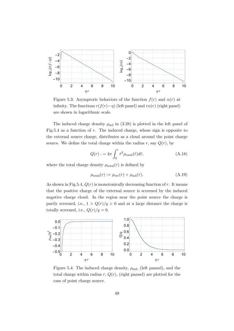
The induced charge density ρind in (3.28) is plotted in the left panel of
Fig.5.4 as a function of r. The induced charge, whose sign is opposite to
the external source charge, distributes as a cloud around the point charge
source. We define the total charge within the radius r, say Q(r), by
Q(r) : = 4π
∫ r
0r2ρtotal(r)dr, (A.18)
where the total charge density ρtotal(r) is defined by
ρtotal(r) := ρext(r) + ρind(r). (A.19)
As shown in Fig.5.4, Q(r) is monotonically decreasing function of r. It means
that the positive charge of the external source is screened by the induced
negative charge cloud. In the region near the point source the charge is
partly screened, i.e., 1 > Q(r)/q > 0 and at a large distance the charge is
totally screened, i.e., Q(r)/q = 0.
0 2 4 6 8 10-0.5
-0.4
-0.3
-0.2
-0.1
0.0
η r
ρind/η3
0 2 4 6 8 100.0
0.2
0.4
0.6
0.8
1.0
η r
Q/q
Figure 5.4: The induced charge density, ρind, (left pannel), and the
total charge within radius r, Q(r), (right pannel) are plotted for the
case of point charge source.
49
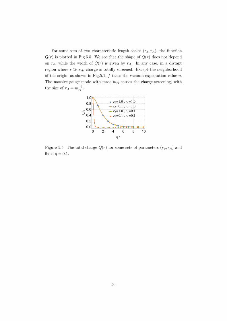
For some sets of two characteristic length scales (rϕ, rA), the function
Q(r) is plotted in Fig.5.5. We see that the shape of Q(r) does not depend
on rϕ, while the width of Q(r) is given by rA. In any case, in a distant
region where r ≫ rA, charge is totally screened. Except the neighborhood
of the origin, as shown in Fig.5.1, f takes the vacuum expectation value η.
The massive gauge mode with mass mA causes the charge screening, with
the size of rA = m−1A .
rϕ=1.0 , rA=1.0 rϕ=0.1 , rA=1.0 rϕ=1.0 , rA=0.1 rϕ=0.1 , rA=0.1
0 2 4 6 8 100.0
0.2
0.4
0.6
0.8
1.0
η r
Q/q
Figure 5.5: The total charge Q(r) for some sets of parameters (rϕ, rA) and
fixed q = 0.1.
50
Appendix B Approximate solutions for the Gaus-
sian distribution sources
First, we consider the thin source case, rs ≪ rA. As shown in the first panel
of Fig.3.1 and Fig.3.3 for the case rs = 0.1 as an example, we see
|ρind| = 2e2f2α≪ ρext and η2 < f2 ≪ α2 (B.1)
in the near region, 0 ≤ r ≤ rs. Then, (3.29) and (3.30) reduces to
d2f
dr2+
2
r
df
dr+ α2f = 0, (B.2)
d2α
dr2+
2
r
dα
dr+ ρ0 exp
[−(r
rs
)2]= 0. (B.3)
in this region. We easily find a set of approximate solutions that satisfies
the boundary condition (3.39) in the expansion form
α(r) = α0 −ρ0r
2s
6
(r
rs
)2
+O(r
rs
)4
, (B.4)
f(r) = f0
(1− α2
0r2s
6
(r
rs
)2
+O(r
rs
)4), (B.5)
where α0 := α(0) and f0 := f(0).
In the far region, r ≫ rs, the functions f and α take the same forms of
the point source case. The constants soliton α0 and f0 should be adjusted
so that the solutions are smoothly connected from the near region to the far
region.
Next, we consider the thick source case, rs ≫ rA. Since the source is
spread widely, the variation of the external charge density is very small.
Accordingly, the variation of the functions f and α are also small as is seen
in the last panel of Fig.3.1 as an example. Then the derivative terms in
(3.29) and (3.30) can be negligible, and we have
− 2e2α2 + λ(f2 − η2) = 0, (B.6)
ρind = −ρext. (B.7)
If the external charge density ρext is small such that
ρext ≪η
rA rϕ, (B.8)
51
we have
f ≃ η, and α ≃ ρextm2A
. (B.9)
This behavior is seen in the last panel of Fig.3.1.
52
Appendix C Approximate solutions for the homo-
geneous ball sources
In the homogeneous ball sources with rs ≫ rA, except the vicinity of the
ball surface, rs − rA < r < rs + rA, f and α are almost constants soliton.
We can approach approximately to this simple behaviors.
In the region r < rs − rA, where ρext ≃ ρ0 = const., since the derivative
terms in (3.30) and (3.29) can be ignored for the solutions that satisfy the
boundary condition (3.39), then f and α take constant values. The equations
of motion reduce to
e2fα2 − λ
2f(f2 − η2) = 0, (C.1)
− 2e2f2α+ ρ0 = 0. (C.2)
By solving these coupled algebraic equations, we obtain
f2 ≃ f20 =1
3η2[1 +
(1 +X +
√X(2 +X)
)1/3+(1 +X +
√X(2 +X)
)−1/3],
(C.3)
α ≃ α0 =ρ0
2e2f20, (C.4)
where X is the constant defined by
X :=27rArϕ
2ηρ0. (C.5)
In the region r ≥ rs + rA, where ρext ≃ 0, we have simply f ≃ η and α ≃ 0.
The fields f and α change their values quickly in the vicinity of the ball
surface.
If ρ0 ≪ η/(rϕrA), a global solution can be obtained approximately. In
this case, as same as the Gaussian source case, f(r) ∼ η. Moreover, if
ζs ≪ rA, the equation of the gauge field can be reduced to
d2α
dr2+
2
r
dα
dr−m2
Aα+ ρ0θ(rs − r) = 0, (C.6)
where mA = r−1A . This is the Proca equation for a homogenious ball source.
In the region r < rs, since ρext(r) = ρ0, we have a solution
α(r) =C1
rsinh (r/rA) + ρ0r
2A, (C.7)
53
while in the region r > rs, we have
α(r) =C2
rexp (−r/rA) , (C.8)
where C1 and C2 are constants soliton that should be determined by con-
tinuity. This is achieved by junction conditions for (C.7) and (C.8) at the
surface r = rs as
C2 exp(−rs/rA) = C1 sinh(rs/rA) + ρ0rsr2A, (C.9)
−C2 exp(−rs/rA)(1 +
rsrA
)= C1
[rsrA
cosh(rs/rA)− sinh(rs/rA)
].
(C.10)
By solving (C.9) and (C.10), we obtain
C1 = −ρ0r
3A
(1 + rs
rA
)cosh(rs/rA) + sinh(rs/rA)
, (C.11)
C2 =ρ0r
3A exp(rs/rA)
[rsrA
cosh(rs/rA)− sinh(rs/rA)]
cosh(rs/rA) + sinh(rs/rA). (C.12)
Another simple case is that of ζs ≫ rA. The derivative terms in (3.30)
and (3.29) can be ignored everywhere for the solutions that satisfy the
boundary conditions (3.39) and (3.40), then the equations of motion reduce
to
e2fα2 − λ
2f(f2 − η2) = 0, (C.13)
− 2e2f2α+ ρext = 0. (C.14)
Therefore,
f2(r) ≃ 1
3η2[1 +
(1 + Y (r) +
√Y (r)(2 + Y (r))
)1/3+(1 + Y (r) +
√Y (r)(2 + Y (r))
)−1/3],
(C.15)
α(r) ≃ ρext(r)
2e2f(r)2, (C.16)
where Y (r) is the function defined by
Y (r) :=27rArϕ
2ηρext(r). (C.17)
54
Appendix D Energy-Momentum Tensor of the Sys-
tem
The energy-momentum tensor Tµν of the present system is given by
Tµν =2(Dµψ)∗(Dνψ)− gµν(Dαψ)
∗(Dαψ)
+ 2(Dµϕ)∗(Dνϕ)− gµν(Dαϕ)
∗(Dαϕ)
− gµν (V (ϕ) + µψ∗ψϕ∗ϕ)
+
(FµαF
αν − 1
4gµνFαβF
αβ
). (D.1)
Energy density and pressure components soliton are given by
ϵ =− T tt
= |Dtψ|2 + (Diψ)∗(Diψ) + |Dtϕ|2 + (Diϕ)
∗(Diϕ)
+ V (ϕ) + µ|ψ|2|ϕ|2 + 1
2
(EiE
i +BiBi), (D.2)
pr =Trr
=(Drψ)∗(Drψ) + |Dtψ|2 − (Dθψ)
∗(Dθψ)− (Dφψ)∗(Dφψ)
+ (Drϕ)∗(Drϕ) + |Dtϕ|2 − (Dθϕ)
∗(Dθϕ)− (Dφϕ)∗(Dφϕ)
− V (ϕ)− µ|ψ|2|ϕ|2
+1
2(−ErEr + EθE
θ + EφEφ −BrB
r +BθBθ +BφB
φ), (D.3)
pθ =Tθθ
=(Dθψ)∗(Dθψ) + |Dtψ|2 − (Drψ)
∗(Drψ)− (Dφψ)∗(Dφψ)
+ (Dθϕ)∗(Dθϕ) + |Dtϕ|2 − (Drϕ)
∗(Drϕ)− (Dφϕ)∗(Dφϕ)
− V (ϕ)− µ|ψ|2|ϕ|2
+1
2(−EθEθ + ErE
r + EφEφ −BθB
θ +BrBr +BφB
φ), (D.4)
pφ =Tφφ
=(Dφψ)∗(Dφψ) + |Dtψ|2 − (Drψ)
∗(Drψ)− (Dθψ)∗(Dθψ)
+ (Dφϕ)∗(Dφϕ) + |Dtϕ|2 − (Drϕ)
∗(Drϕ)− (Dθϕ)∗(Dθϕ)
− V (ϕ)− µ|ψ|2|ϕ|2
+1
2(−EφEφ + ErE
r + EθEθ −BφB
φ +BrBr +BθB
θ). (D.5)
55
Appendix E Other bounce solutions
E.1 Stationary Points of the System and Bounce Solutions
By solving (4.39), we can find stationary points. In addition to the isolated
stationary points Pv and P0, there exist ridges, R1 and R2, each ridge con-
sists of infinite stationary points aligned on a line, in the region u ≥ 0, f ≥ 0,
and α ≥ 0. The ridges are sets of points
R1 : α1 =Ω
e, f1 = 0, u1 = arbitrarly constants, (E.1)
R2 : α2 = arbitrarly constants, f2 = 0, u2 = 0. (E.2)
In addition to the bounce solution of the type P0 → Pv, we find numerical
bounce solutions of the type
P1 → Pv and Pv → Pv, (E.3)
where P1 is a point in the ridge R1. For any stationary point P2 in the ridge
R2, there is no solution of the type P2 → Pv.
E.2 Numerical calculations
Trajectories of the three solutions, P0 → Pv, P1 → Pv, and Pv → Pv, in
(u, f, α) space are shown in Fig.5.6.
56
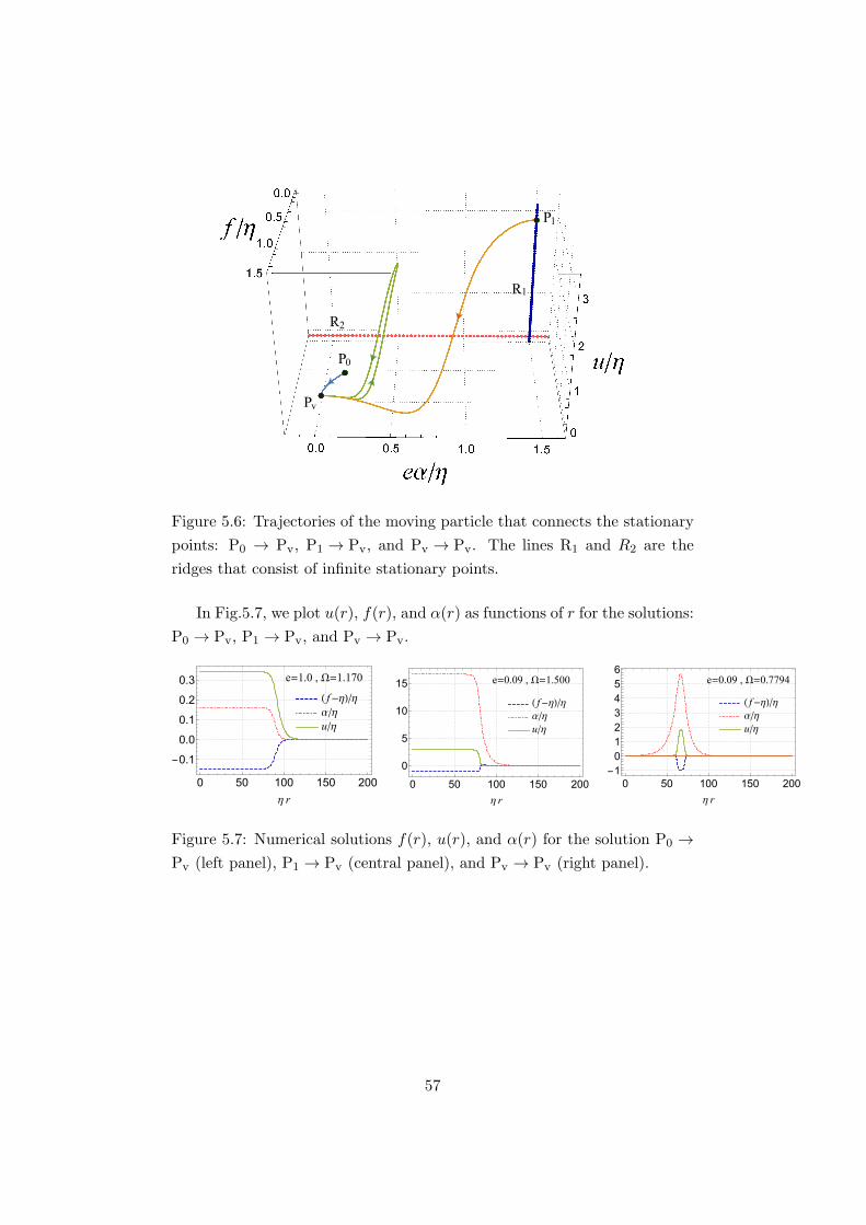
Pv
P0
P1
R1
R2
Figure 5.6: Trajectories of the moving particle that connects the stationary
points: P0 → Pv, P1 → Pv, and Pv → Pv. The lines R1 and R2 are the
ridges that consist of infinite stationary points.
In Fig.5.7, we plot u(r), f(r), and α(r) as functions of r for the solutions:
P0 → Pv, P1 → Pv, and Pv → Pv.
( f-η)/η
α/η
u/η
0 50 100 150 200
-0.1
0.0
0.1
0.2
0.3
η r
e=1.0 , Ω=1.170
( f-η)/η
α/η
u/η
0 50 100 150 200
0
5
10
15
η r
e=0.09 , Ω=1.500
( f-η)/η
α/η
u/η
0 50 100 150 200-10123456
η r
e=0.09 , Ω=0.7794
Figure 5.7: Numerical solutions f(r), u(r), and α(r) for the solution P0 →Pv (left panel), P1 → Pv (central panel), and Pv → Pv (right panel).
57
Bibliography
[1] H. B. Nielsen and P. Olesen, “Vortex Line Models for Dual Strings,”
Nucl. Phys. B 61, 45 (1973).
[2] G. ’t Hooft, “Magnetic Monopoles in Unified Gauge Theories,” Nucl.
Phys. B 79, 276 (1974).
[3] A. Vilenkin, “Cosmic Strings And Other Topological Defects,”
[4] G. Rosen, “Particlelike Solutions to Nonlinear Complex Scalar Field
Theories with Positive‐ Definite Energy Densities,” J. Math. Phys. 9,
996 (1968).
[5] G. Rosen, “Charged Particlelike Solutions to Nonlinear Complex
Scalar Field Theories,” J. Math. Phys. 9, 999 (1968).
[6] R. Friedberg, T. D. Lee and A. Sirlin, “A Class of Scalar-Field Soliton
Solutions in Three Space Dimensions,” Phys. Rev. D 13, 2739 (1976).
[7] S. R. Coleman, “Q Balls,” Nucl. Phys. B 262, 263 (1985) Erratum:
[Nucl. Phys. B 269, 744 (1986)].
[8] A. Kusenko, “Solitons in the supersymmetric extensions of the stan-
dard model,” Phys. Lett. B 405, 108 (1997).
[9] A. Kusenko, “Q balls in the MSSM,” Nucl. Phys. Proc. Suppl. 62A/C,
248 (1998) doi:10.1016/S0920-5632(97)00664-6 [hep-ph/9707306].
[10] S. Kasuya and M. Kawasaki, “A New type of stable Q balls in the
gauge mediated SUSY breaking,” Phys. Rev. Lett. 85, 2677 (2000).
[11] G. R. Dvali, A. Kusenko and M. E. Shaposhnikov, “New physics in a
nutshell, or Q ball as a power plant,” Phys. Lett. B 417, 99 (1998).
58
[12] A. Kusenko and M. E. Shaposhnikov, “Supersymmetric Q balls as
dark matter,” Phys. Lett. B 418, 46 (1998).
[13] A. Kusenko and P. J. Steinhardt, “Q ball candidates for selfinteracting
dark matter,” Phys. Rev. Lett. 87, 141301 (2001).
[14] M. Fujii and K. Hamaguchi, “Higgsino and wino dark matter from Q
ball decay,” Phys. Lett. B 525, 143 (2002).
[15] K. Enqvist, A. Jokinen, T. Multamaki and I. Vilja, “Constraints on
selfinteracting Q ball dark matter,” Phys. Lett. B 526, 9 (2002).
[16] A. Kusenko, L. Loveridge and M. Shaposhnikov, “Supersymmetric
dark matter Q-balls and their interactions in matter,” Phys. Rev. D
72, 025015 (2005).
[17] K. Enqvist and J. McDonald, “Q balls and baryogenesis in the
MSSM,” Phys. Lett. B 425, 309 (1998).
[18] S. Kasuya and M. Kawasaki, “Q ball formation through Affleck-Dine
mechanism,” Phys. Rev. D 61, 041301 (2000).
[19] M. Kawasaki, F. Takahashi and M. Yamaguchi, “Large lepton asym-
metry from Q balls,” Phys. Rev. D 66, 043516 (2002).
[20] K. M. Lee, J. A. Stein-Schabes, R. Watkins and L. M. Widrow,
“Gauged q Balls,” Phys. Rev. D 39, 1665 (1989).
[21] X. Shi and X. Z. Li, ”Nontopological solitons in a U(1) gauge theory,”
J. Phys. A 24, 4075 (1991).
[22] I. E. Gulamov, E. Y. Nugaev, A. G. Panin and M. N. Smolyakov,
“Some properties of U(1) gauged Q-balls,” Phys. Rev. D 92, no. 4,
045011 (2015).
[23] H. Arodz and J. Lis, “Compact Q-balls and Q-shells in a scalar elec-
trodynamics,” Phys. Rev. D 79, 045002 (2009).
[24] T. Tamaki and N. Sakai, “Large gauged Q-balls with regular poten-
tial,” Phys. Rev. D 90, 085022 (2014).
59
[25] H. Ishihara and T. Ogawa, “Charge Screened Nontopological Soli-
tons in a Spontaneously Broken U(1) Gauge Theory“ arXiv:1811.10894
[hep-th], Prog. Theor. Exp. Phys. 2019, 021B01 (2019).
[26] H. Ishihara and T. Ogawa, “Perfect Charge Screening of Extended
Sources in an Abelian-Higgs Model,” arXiv:1811.10848 [hep-th].
[27] H. Ishihara and T. Ogawa, “Homogeneous Balls in a Spontaneously
Broken U(1) Gauge Theory,“ arXiv:1901.08799 [hep-th]., Phys. Rev.
D 99, 056019 (2019).
[28] M. Deshaies-Jacques and R. MacKenzie, “Maxwell-Chern-Simons
Q-balls,” Can. J. Phys. 85, 693 (2007) doi:10.1139/p07-063 [hep-
th/0606258].
[29] K. N. Anagnostopoulos, M. Axenides, E. G. Floratos and N. Tetradis,
“Large gauged Q balls,” Phys. Rev. D 64, 125006 (2001).
[30] A. G. Cohen, S. R. Coleman, H. Georgi and A. Manohar, “The Evap-
oration of Q Balls,” Nucl. Phys. B 272, 301 (1986).
[31] A. Kusenko, “Small Q balls,” Phys. Lett. B 404, 285 (1997).
[32] T. Multamaki and I. Vilja, “Analytical and numerical properties of Q
balls,” Nucl. Phys. B 574, 130 (2000).
[33] F. Paccetti Correia and M. G. Schmidt, “Q balls: Some analytical
results,” Eur. Phys. J. C 21, 181 (2001).
[34] M. Kawasaki, K. Konya and F. Takahashi, “Q-ball instability due to
U(1) breaking,” Phys. Lett. B 619, 233 (2005).
[35] N. Sakai and M. Sasaki, ”Stability of Q-balls and Catastrophe,” Prog.
Theor. Phys. 119, 929 (2008).
[36] R. Friedberg, T. D. Lee and Y. Pang, “Mini - Soliton Stars,” Phys.
Rev. D 35, 3640 (1987).
[37] R. Friedberg, T. D. Lee and Y. Pang, ”Scalar Soliton Stars and Black
Holes,” Phys. Rev. D 35, 3658 (1987).
[38] T. D. Lee and Y. Pang, “Fermion Soliton Stars and Black Holes,”
Phys. Rev. D 35, 3678 (1987).
60
[39] B. W. Lynn, “Q Stars,” Nucl. Phys. B 321, 465 (1989).
[40] D. F. Torres, S. Capozziello and G. Lambiase, “A Supermassive scalar
star at the galactic center?,” Phys. Rev. D 62, 104012 (2000)
[41] E. W. Mielke and F. E. Schunck, “Nontopological scalar soliton as
dark matter halo,” Phys. Rev. D 66, 023503 (2002).
[42] F. E. Schunck and E. W. Mielke, “General relativistic boson stars,”
Class. Quant. Grav. 20, R301 (2003)
[43] J. A. Frieman, G. B. Gelmini, M. Gleiser and E. W. Kolb, “Solitogen-
esis: Primordial Origin of Nontopological Solitons,” Phys. Rev. Lett.
60, 2101 (1988).
[44] K. Griest and E. W. Kolb, “Solitosynthesis: Cosmological Evolution
of Nontopological Solitons,” Phys. Rev. D 40, 3231 (1989).
[45] S. Kasuya and M. Kawasaki, “Q Ball formation in the gravity medi-
ated SUSY breaking scenario,” Phys. Rev. D 62, 023512 (2000).
[46] M. Postma, “Solitosynthesis of Q balls,” Phys. Rev. D 65, 085035
(2002).
[47] T. Multamaki and I. Vilja, “Simulations of Q ball formation,” Phys.
Lett. B 535, 170 (2002).
[48] T. Hiramatsu, M. Kawasaki and F. Takahashi, “Numerical study of
Q-ball formation in gravity mediation,” JCAP 1006, 008 (2010).
[49] R. Friedberg and T. D. Lee, ”Fermion Field Nontopological Solitons.
1.,” Phys. Rev. D 15, 1694 (1977).
[50] R. Friedberg and T. D. Lee, “Fermion Field Nontopological Solitons.
2. Models for Hadrons,” Phys. Rev. D 16, 1096 (1977).
[51] K. Shima, ”Charge Screening and an Extended Model of Hadrons,”
Nuovo Cim. A 44, 163 (1978).
[52] T. S. Levi and M. Gleiser, “Gauged fermionic Q balls,” Phys. Rev. D
66, 087701 (2002).
[53] J. E. Mandula, “Total Charge Screening,” Phys. Lett. 69B, 495
(1977).
61
[54] M. Bawin and J. Cugnon, “Charge Screening In Classical Scalar Elec-
trodynamics,” Phys. Rev. D 37, 2344 (1988).
[55] P. Sikivie and N. Weiss, “Screening Solutions To Classical Yang-mills
Theory,” Phys. Rev. Lett. 40, 1411 (1978).
[56] W. B. Campbell and R. E. Norton, “Total source charge and charge
screening in Yang-Mills theories,” Phys. Rev. D 44, 3931 (1991).
[57] L.D. Landau and E.M. Lifschitz, “Quantum mechanics”, Pergamon
Press (1965)
[58] S. L. Adler and T. Piran, “Relaxation Methods for Gauge field Equi-
librium Equations,” Rev. Mod. Phys. 56, 1 (1984).
62