1

Notes on “Learning about a new technology: Pineapples in Ghana” by T. Conley and C. Udry

Technology adoption is fundamental to development Characteristics of technology usually not transparent to new user – an investment in learning required Multiple adopters in similar circumstances (often case with innovation in agriculture): • process of learning may be social • learn of characteristics from each other

Role of social learning has been studied theoretically • Endogenous growth literature

Only recently tried to measure quantitative importance of learning from others – peer effects literature Important from policy perspective – encourage policies which spread externalities to learning This paper investigates role of social learning in diffusion of new agricultural technology in Ghana

2

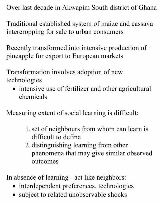
Over last decade in Akwapim South district of Ghana Traditional established system of maize and cassava intercropping for sale to urban consumers Recently transformed into intensive production of pineapple for export to European markets Transformation involves adoption of new technologies • intensive use of fertilizer and other agricultural

chemicals Measuring extent of social learning is difficult:

1. set of neighbours from whom can learn is difficult to define

2. distinguishing learning from other phenomena that may give similar observed outcomes

In absence of learning - act like neighbors: • interdependent preferences, technologies • subject to related unobservable shocks

3

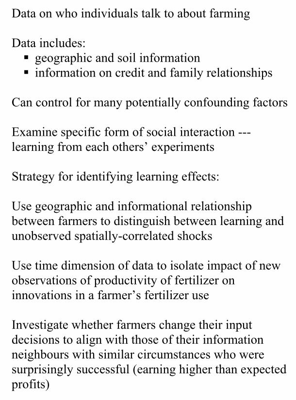
Data on who individuals talk to about farming Data includes:

geographic and soil information information on credit and family relationships

Can control for many potentially confounding factors Examine specific form of social interaction --- learning from each others’ experiments Strategy for identifying learning effects: Use geographic and informational relationship between farmers to distinguish between learning and unobserved spatially-correlated shocks Use time dimension of data to isolate impact of new observations of productivity of fertilizer on innovations in a farmer’s fertilizer use Investigate whether farmers change their input decisions to align with those of their information neighbours with similar circumstances who were surprisingly successful (earning higher than expected profits)

4

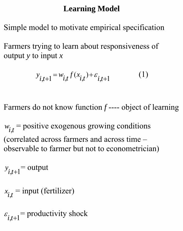
Learning Model

Simple model to motivate empirical specification Farmers trying to learn about responsiveness of output y to input x

1,),(,1, ++=+ titixftiwtiy ε (1)

Farmers do not know function f ---- object of learning

tiw , = positive exogenous growing conditions (correlated across farmers and across time – observable to farmer but not to econometrician)

1, +tiy = output

tix , = input (fertilizer)

1, +tiε = productivity shock

5

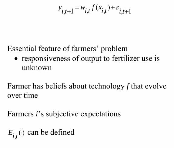
1,),(,1, ++=+ titixftiwtiy ε

Essential feature of farmers’ problem • responsiveness of output to fertilizer use is

unknown Farmer has beliefs about technology f that evolve over time Farmers i’s subjective expectations

)(, ⋅tiE can be defined

6

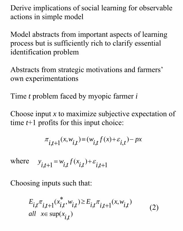
Derive implications of social learning for observable actions in simple model Model abstracts from important aspects of learning process but is sufficiently rich to clarify essential identification problem Abstracts from strategic motivations and farmers’ own experimentations Time t problem faced by myopic farmer i Choose input x to maximize subjective expectation of time t+1 profits for this input choice:

pxtixftiwtiwxti −+≡+ ),)(,(),,(1, επ

where 1,),(,1, ++=+ titixftiwtiy ε

Choosing inputs such that:

),sup(

),,(1,,),,*,(1,,

tixxalltiwxtitiEtiwtixtitiE

∈+≥+ ππ

(2)

7

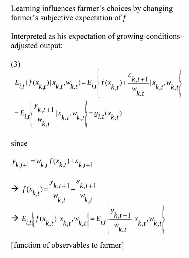
Learning influences farmer’s choices by changing farmer’s subjective expectation of f Interpreted as his expectation of growing-conditions-adjusted output: (3)

),(,,,

,|

,

1,,

,,

,|

,

1,),

(,),,,|),({,

tkxtigtk

wtk

xtk

wtk

ytiE

tkw

tkx

tkwtk

tkxftiEtkwtkxtkxftiE

=+=

++=

⎪⎪⎭

⎪⎪⎬

⎫

⎪⎪⎩

⎪⎪⎨

⎧

⎪⎪⎭

⎪⎪⎬

⎫

⎪⎪⎩

⎪⎪⎨

⎧ ε

since

1,),(,1, ++=+ tktkxftkwtky ε

tk

wtk

tkw

tky

tkxf,

1,

,

1,),( +−+=ε

=⎪⎭

⎪⎬⎫

⎪⎩

⎪⎨⎧

tkwtkxtkxftiE ,,,|),(,⎪⎪⎭

⎪⎪⎬

⎫

⎪⎪⎩

⎪⎪⎨

⎧

+tkwtkx

tkw

tky

tiE ,,,|,

1,,

[function of observables to farmer]

8

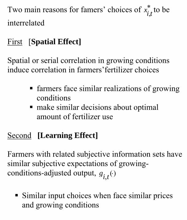
Two main reasons for famers’ choices of *,tix to be

interrelated

First [Spatial Effect] Spatial or serial correlation in growing conditions induce correlation in farmers’fertilizer choices

farmers face similar realizations of growing conditions

make similar decisions about optimal amount of fertilizer use

Second [Learning Effect] Farmers with related subjective information sets have similar subjective expectations of growing-conditions-adjusted output, )(, ⋅tig

Similar input choices when face similar prices and growing conditions

9

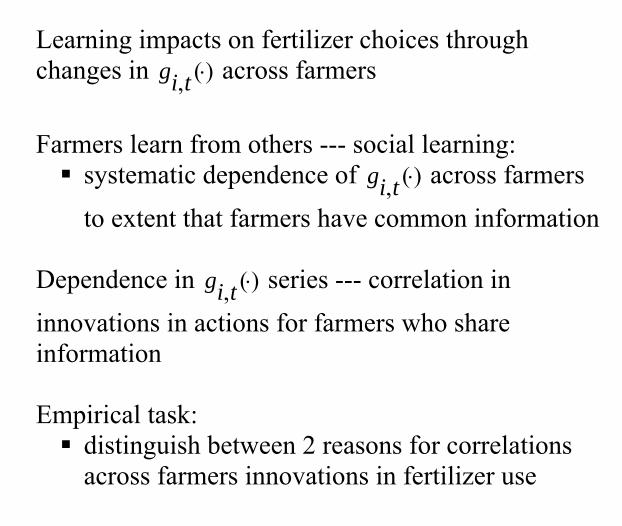
Learning impacts on fertilizer choices through changes in )(, ⋅tig across farmers Farmers learn from others --- social learning:

systematic dependence of )(, ⋅tig across farmers to extent that farmers have common information

Dependence in )(, ⋅tig series --- correlation in innovations in actions for farmers who share information Empirical task:

distinguish between 2 reasons for correlations across farmers innovations in fertilizer use

10

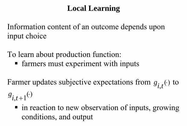
Local Learning Information content of an outcome depends upon input choice To learn about production function:

farmers must experiment with inputs

Farmer updates subjective expectations from )(, ⋅tig to )(1, ⋅+tig

in reaction to new observation of inputs, growing conditions, and output

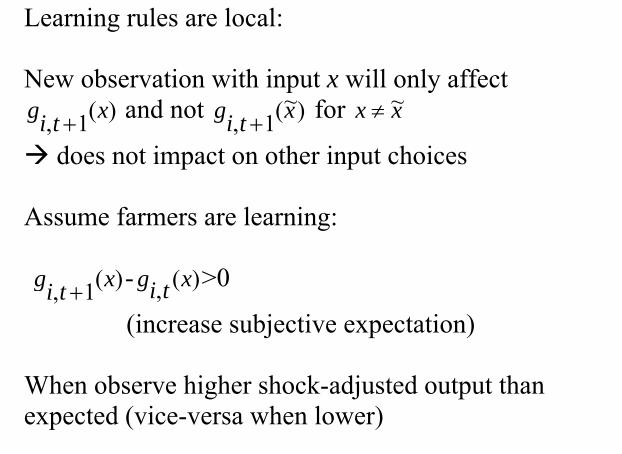
Learning rules are local: New observation with input x will only affect

)(1, xtig + and not )~(1, xtig + for x ≠ x~

does not impact on other input choices Assume farmers are learning: )(1, xtig + - )(, xtig >0

(increase subjective expectation) When observe higher shock-adjusted output than expected (vice-versa when lower)

10

Local Learning Information content of an outcome depends upon input choice To learn about production function:

farmers must experiment with inputs

Farmer updates subjective expectations from )(, ⋅tig to )(1, ⋅+tig

in reaction to new observation of inputs, growing conditions, and output

Learning rules are local: New observation with input x will only affect

)(1, xtig + and not )~(1, xtig + for x ≠ x~

does not impact on other input choices Assume farmers are learning: )(1, xtig + - )(, xtig >0

(increase subjective expectation) When observe higher shock-adjusted output than expected (vice-versa when lower)

11

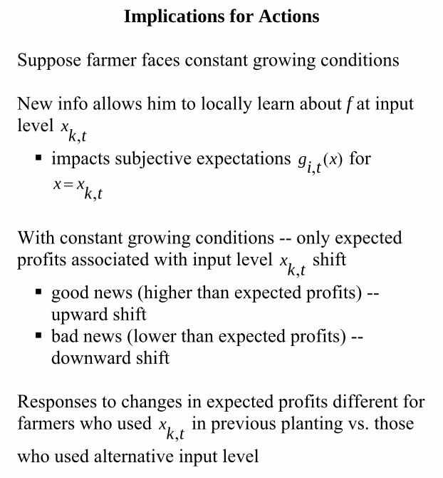
Implications for Actions

Suppose farmer faces constant growing conditions New info allows him to locally learn about f at input level tkx ,

impacts subjective expectations )(, xtig for

tkxx ,=

With constant growing conditions -- only expected profits associated with input level tkx , shift

good news (higher than expected profits) -- upward shift

bad news (lower than expected profits) -- downward shift

Responses to changes in expected profits different for farmers who used tkx , in previous planting vs. those

who used alternative input level

12

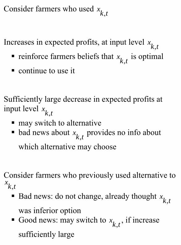
Consider farmers who used tkx ,

Increases in expected profits, at input level tkx ,

reinforce farmers beliefs that tkx , is optimal

continue to use it Sufficiently large decrease in expected profits at input level tkx ,

may switch to alternative bad news about tkx , provides no info about

which alternative may choose Consider farmers who previously used alternative to

tkx ,

Bad news: do not change, already thought tkx ,

was inferior option Good news: may switch to tkx , , if increase

sufficiently large

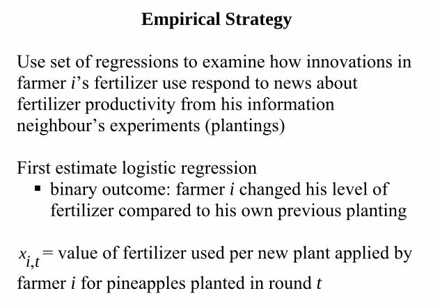
13

Empirical Strategy Use set of regressions to examine how innovations in farmer i’s fertilizer use respond to news about fertilizer productivity from his information neighbour’s experiments (plantings) First estimate logistic regression

binary outcome: farmer i changed his level of fertilizer compared to his own previous planting

tix , = value of fertilizer used per new plant applied by

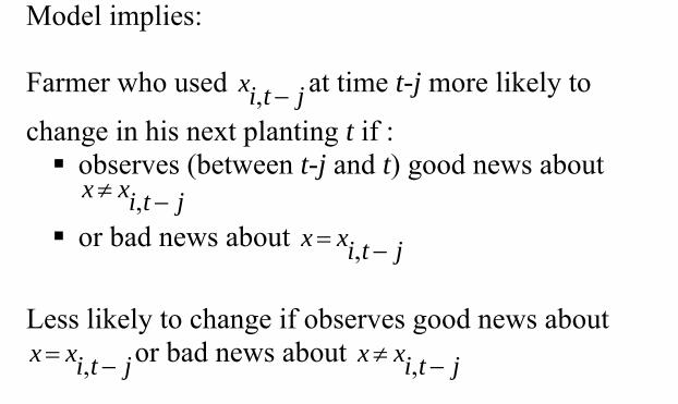
farmer i for pineapples planted in round t Model implies: Farmer who used jtix −, at time t-j more likely to

change in his next planting t if : observes (between t-j and t) good news about

jtixx −≠ ,

or bad news about jtixx −= ,

Less likely to change if observes good news about

jtixx −= , or bad news about jtixx −≠ ,

13

Empirical Strategy Use set of regressions to examine how innovations in farmer i’s fertilizer use respond to news about fertilizer productivity from his information neighbour’s experiments (plantings) First estimate logistic regression

binary outcome: farmer i changed his level of fertilizer compared to his own previous planting

tix , = value of fertilizer used per new plant applied by

farmer i for pineapples planted in round t Model implies: Farmer who used jtix −, at time t-j more likely to

change in his next planting t if : observes (between t-j and t) good news about

jtixx −≠ ,

or bad news about jtixx −= ,

Less likely to change if observes good news about

jtixx −= , or bad news about jtixx −≠ ,

14

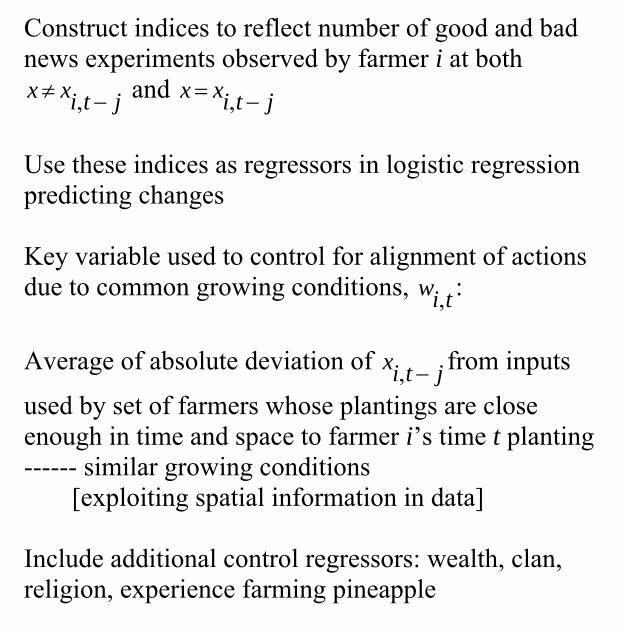
Construct indices to reflect number of good and bad news experiments observed by farmer i at both

jtixx −≠ , and jtixx −= ,

Use these indices as regressors in logistic regression predicting changes Key variable used to control for alignment of actions due to common growing conditions, tiw , : Average of absolute deviation of jtix −, from inputs

used by set of farmers whose plantings are close enough in time and space to farmer i’s time t planting ------ similar growing conditions [exploiting spatial information in data] Include additional control regressors: wealth, clan, religion, experience farming pineapple

15

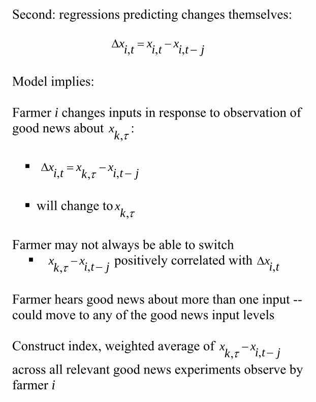
Second: regressions predicting changes themselves:

jtixtixtix −−=Δ ,,,

Model implies: Farmer i changes inputs in response to observation of good news about τ,kx :

jtixkxtix −−=Δ ,,, τ

will change to τ,kx

Farmer may not always be able to switch

jtixkx −− ,,τ positively correlated with tix ,Δ

Farmer hears good news about more than one input -- could move to any of the good news input levels Construct index, weighted average of jtixkx −− ,,τ

across all relevant good news experiments observe by farmer i

16

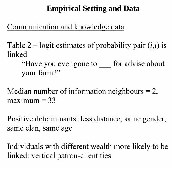
Empirical Setting and Data Communication and knowledge data Table 2 – logit estimates of probability pair (i,j) is linked

“Have you ever gone to ___ for advise about your farm?”

Median number of information neighbours = 2, maximum = 33 Positive determinants: less distance, same gender, same clan, same age Individuals with different wealth more likely to be linked: vertical patron-client ties

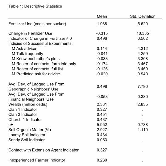
Table 1: Descriptive Statistics

Mean Std. Deviation

Fertilizer Use (cedis per sucker) 1.938 5.620

Change in Fertilizer Use -0.315 10.335Indicator of Change in Fertilizer ≠ 0 0.496 0.502Indicies of Successful Experiments: M Ask advice 0.114 4.312 M Talk frequently -0.041 4.259 M Know each other's plots -0.033 3.308 M Roster of contacts, farm info only -0.174 3.467 M Roster of contacts, full list -0.126 3.469 M Predicted ask for advice -0.020 0.940

Wealth (million cedis) 2.331 2.835Clan 1 Indicator 0.327 .Clan 2 Indicator 0.451 .Church 1 Indicator 0.487 .pH 5.952 0.738Soil Organic Matter (%) 2.927 1.110Loamy Soil Indicator 0.434 .Sandy Soil Indicator 0.053 .

Contact with Extension Agent Indicator 0.327 .

Inexperienced Farmer Indicator 0.230 .

Avg. Dev. of Lagged Use From Geographic Neighbors' UseAvg. Dev. of Lagged Use From Financial Neighbors' Use

0.498 7.790

-0.053 0.380

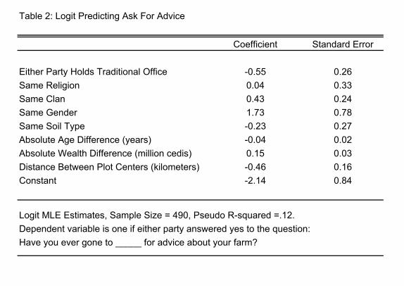
Table 2: Logit Predicting Ask For Advice

Coefficient Standard Error

Either Party Holds Traditional Office -0.55 0.26Same Religion 0.04 0.33Same Clan 0.43 0.24Same Gender 1.73 0.78Same Soil Type -0.23 0.27Absolute Age Difference (years) -0.04 0.02Absolute Wealth Difference (million cedis) 0.15 0.03Distance Between Plot Centers (kilometers) -0.46 0.16Constant -2.14 0.84

Logit MLE Estimates, Sample Size = 490, Pseudo R-squared =.12.Dependent variable is one if either party answered yes to the question:Have you ever gone to _____ for advice about your farm?

19

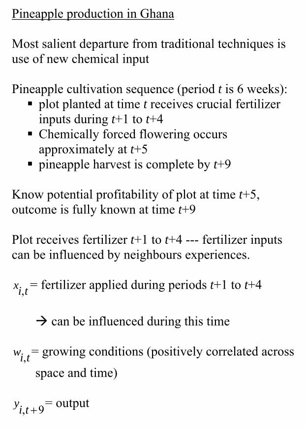
Pineapple production in Ghana Most salient departure from traditional techniques is use of new chemical input Pineapple cultivation sequence (period t is 6 weeks):

plot planted at time t receives crucial fertilizer inputs during t+1 to t+4

Chemically forced flowering occurs approximately at t+5

pineapple harvest is complete by t+9 Know potential profitability of plot at time t+5, outcome is fully known at time t+9 Plot receives fertilizer t+1 to t+4 --- fertilizer inputs can be influenced by neighbours experiences.

tix , = fertilizer applied during periods t+1 to t+4

can be influenced during this time

tiw , = growing conditions (positively correlated across space and time)

9, +tiy = output

20

Periods are sufficiently short --- substantial correlation in soil moisture, weeds, pest conditions on a given plot over time Soil types and topographical features are correlated across neighbours plots but vary within villages Common village-level weather shocks can have varying impact across the village Rainfall realizations can be different on opposite sides of a single village Weeds spread in a continuous manner, soil moisture and pest environments are more similarly on nearby plots Nine period growing cycle -- correlation for physically close plots at different but near points in time (overlap in environmental conditions) Geographic neighbours = within 1 km of geographic center of all farmers pineapple plots median number = 12, max = 25

Pro

porti

on o

f Far

mer

s C

ultiv

atin

g P

inea

pple

'experienced' 'inexperienced'1990 1992 1994 1996 1998

.1

.2

.3

.4

.5

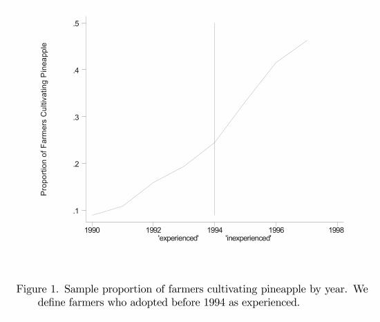
Figure 1. Sample proportion of farmers cultivating pineapple by year. Wedefine farmers who adopted before 1994 as experienced.

54

22

For some of the analysis divide sample into 2 groups: experienced (adopted before 1994) and inexperienced (adopted more recently) Pineapple cultivators are richer, male, more likely to be in each others information neighbourhood

23

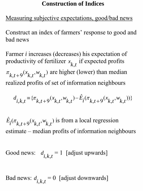
Construction of Indices

Measuring subjective expectations, good/bad news Construct an index of farmers’ response to good and bad news Farmer i increases (decreases) his expectation of productivity of fertilizer tkx , if expected profits

),,,(9, tkwtkxtk +π are higher (lower) than median

realized profits of set of information neighbours

))},,,(9,(ˆ),,,(9,{,, tkwtkxtkiEtkwtkxtktkid +−+≡ ππ

),,,(9,(ˆ

tkwtkxtkiE +π is from a local regression

estimate – median profits of information neighbours Good news: tkid ,, = 1 [adjust upwards]

Bad news: tkid ,, = 0 [adjust downwards]

24

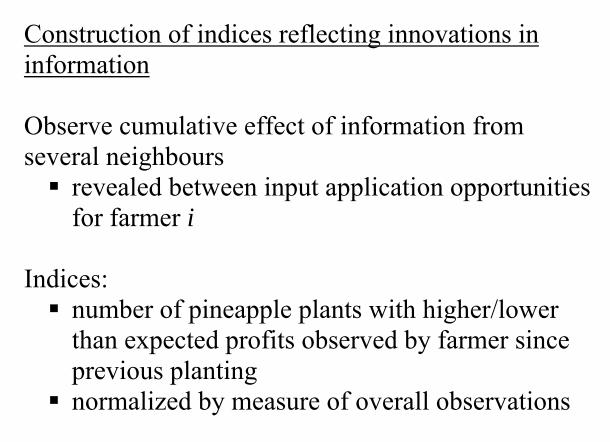
Construction of indices reflecting innovations in information Observe cumulative effect of information from several neighbours

revealed between input application opportunities for farmer i

Indices:

number of pineapple plants with higher/lower than expected profits observed by farmer since previous planting

normalized by measure of overall observations

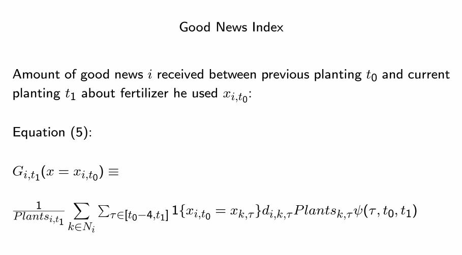
Good News Index

Amount of good news i received between previous planting t0 and current

planting t1 about fertilizer he used xi,t0:

Equation (5):

Gi,t1(x = xi,t0) ≡

1Plantsi,t1

Xk∈Ni

Pτ∈[t0−4,t1] 1{xi,t0 = xk,τ}di,k,τP lantsk,τψ(τ, t0, t1)

Weighted average of number of instances of good news di,k,τ about plant-

ings in i’s information neighbourhood Ni who used xi,t0

Information conveyed depends on number of Plants and ψ(·) which is aweighting function to reflect gradual revelation of information

Assume 1/5 information is revealed in each period t+ 5 to t+ 9

Ad hoc assumption – will examine robustness

Define good news index at alternatives, Gi,t1(x 6= xi,t0) by adjusting indi-

cator function to 1{xi,t0 6= xk,τ}

Define bad new index, Bi,t1(x = xi,t0) and Bi,t1(x 6= xi,t0) by substituting

in 1− di,k,τ

26

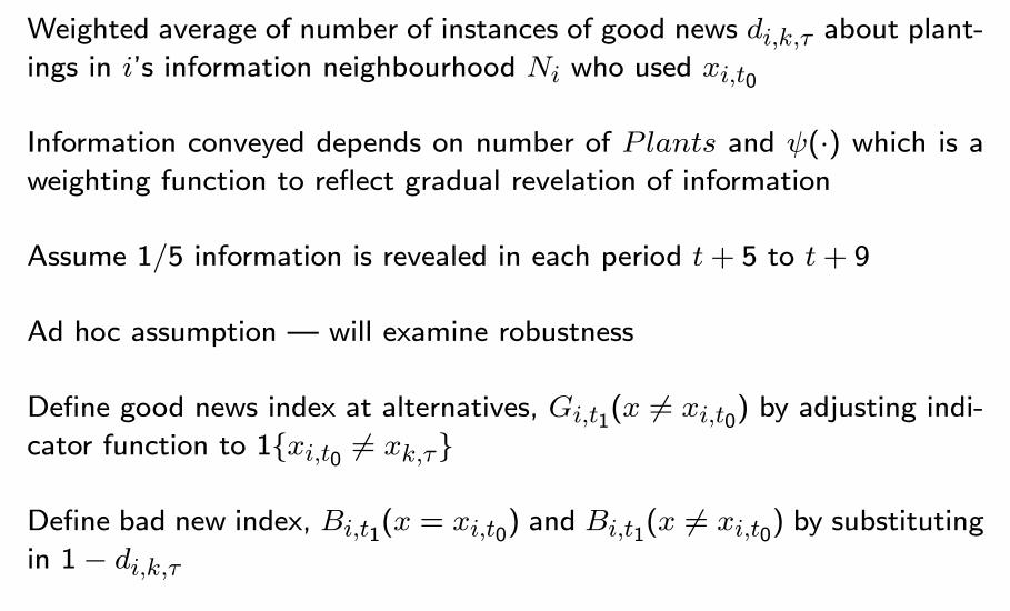
Index of amount of good news that i received between previous planting and current planting about fertilizer he previously used Weighted average of number of instances of good news about plantings by farmers in i’s information neighbourhood who used input level last used by i Information conveyed by information neighbours planting depends on number of plants involved:

weight each observation by Plants Change in beliefs associated with piece of information depends on stock of previous experiments that i has obsrerved

normalize total number plants i observed from beginning of data until current planting

Piecewise linear weighting function reflects gradual revelation of information about harvest:

1/5 relevant info revealed each period t+5 to t+9 ad hoc – examine robustness

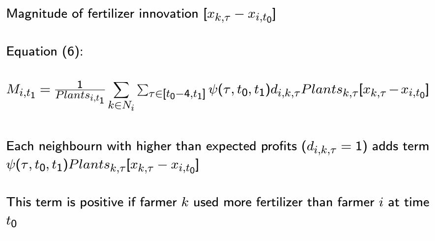
Magnitude of fertilizer innovation [xk,τ − xi,t0]

Equation (6):

Mi,t1 =1

Plantsi,t1

Xk∈Ni

Pτ∈[t0−4,t1]ψ(τ, t0, t1)di,k,τP lantsk,τ [xk,τ −xi,t0]

Each neighbourn with higher than expected profits (di,k,τ = 1) adds term

ψ(τ, t0, t1)Plantsk,τ [xk,τ − xi,t0]

This term is positive if farmer k used more fertilizer than farmer i at time

t0

28

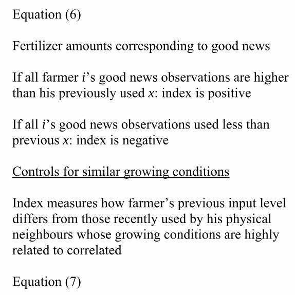
Equation (6) Fertilizer amounts corresponding to good news If all farmer i’s good news observations are higher than his previously used x: index is positive If all i’s good news observations used less than previous x: index is negative Controls for similar growing conditions Index measures how farmer’s previous input level differs from those recently used by his physical neighbours whose growing conditions are highly related to correlated Equation (7)

Equation (7)

Γi,t1 =

1Xk∈NGeo

i

Pτ∈[t0−4,t1] Plantsk,τ

Xk∈NGeo

i

Pτ∈[t0−4,t1]Plantsk,τ [xk,τ − xi,t0]

Geo neighbour is within 1 km radius

Construct also for financial neighbours

30

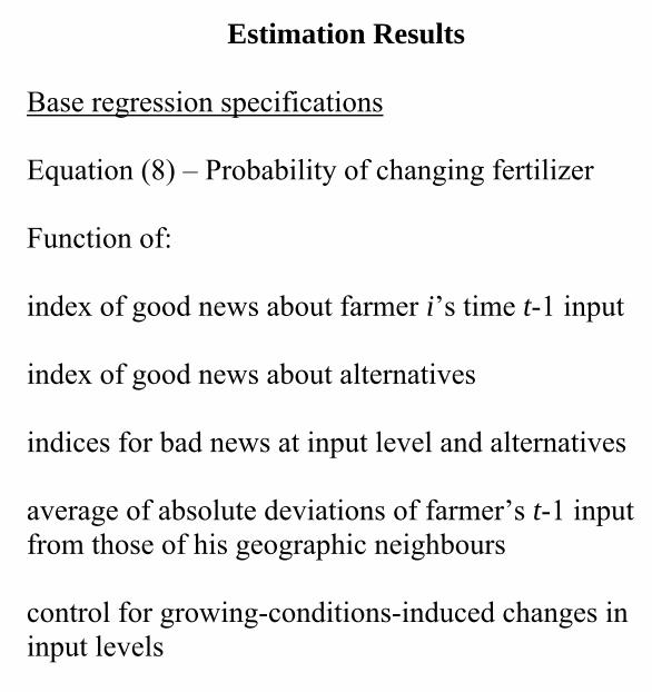
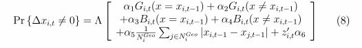
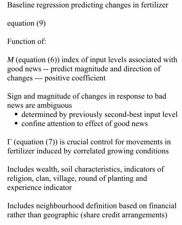
Estimation Results Base regression specifications Equation (8) – Probability of changing fertilizer Function of: index of good news about farmer i’s time t-1 input index of good news about alternatives indices for bad news at input level and alternatives average of absolute deviations of farmer’s t-1 input from those of his geographic neighbours control for growing-conditions-induced changes in input levels

5 Estimation Results

Base Regression SpecificationsThis section presents our base regression specifications. Alternative spec-

ifications and a discussion of robustness are considered in Section 6. Wepresent these specifications as though each farmer has a time t and t − 1planting for simplicity. We let the characteristics of i and his plot that weuse for conditioning be contained in a vector zi,t. These characteristics includethe farmer’s wealth, soil characteristics, and indicators for religion, clan, vil-lage, round of the planting and an indicator that is one if the farmer has beenfarming pineapple for export for less than three years at the start of the sur-vey. Using the notation ∆xi,t for the first difference of inputs, (xi,t−xi,t−1),and the notation Pr {∆xi,t 6= 0} to refer to the probability of changing fer-tilizer use conditional on observable (to the econometrician) information attime t−1, we estimate a logistic specification for this conditional probability:

Pr {∆xi,t 6= 0} = Λ

⎡⎣ α1Gi,t(x = xi,t−1) + α2Gi,t(x 6= xi,t−1)+α3Bi,t(x = xi,t−1) + α4Bi,t(x 6= xi,t−1)+α5

1NGeoi

Pj∈NGeo

i|xi,t−1 − xj,t−1|+ z0i,tα6

⎤⎦ (8)

The first four terms reflect the nature of new information to the farmer.The first term is our index of good news about farmer i0s time t − 1 inputchoice xi,t−1. The second term is the index of good news about alternatives toxi,t−1. The third and fourth terms are the indices of bad news at xi,t−1 and atalternatives to xi,t−1. Local learning implies that α1, α4 < 0 and α2, α3 > 0.The fifth term is the average of absolute deviations of the farmer’s t−1 inputfrom those of his geographic neighbors, our control for growing-conditions-induced changes in input levels. We expect unobserved shocks to growingconditions to be positively spatially and serially correlated and thus α5 > 0.Our baseline regression predicting changes in fertilizer use is:

∆xi,t = β1Mi,t + β2Γi,t + z0i,tβ3 + vi,t. (9)

Mi,t, defined in (6), is our index of input levels associated with good news thatshould predict the magnitude and direction of changes, and should thereforehave a positive coefficient β1. The sign and magnitude of changes in responseto bad news are ambiguous since they are determined by the previouslysecond-best input level. Therefore, we confine our attention to the effectof good news on innovations. Γi,t defined in (7) is our crucial control for

24

31

Baseline regression predicting changes in fertilizer equation (9) Function of: M (equation (6)) index of input levels associated with good news -- predict magnitude and direction of changes --- positive coefficient Sign and magnitude of changes in response to bad news are ambiguous

determined by previously second-best input level confine attention to effect of good news

Г (equation (7)) is crucial control for movements in fertilizer induced by correlated growing conditions Includes wealth, soil characteristics, indicators of religion, clan, village, round of planting and experience indicator Includes neighbourhood definition based on financial rather than geographic (share credit arrangements)

5 Estimation Results

Base Regression SpecificationsThis section presents our base regression specifications. Alternative spec-

ifications and a discussion of robustness are considered in Section 6. Wepresent these specifications as though each farmer has a time t and t − 1planting for simplicity. We let the characteristics of i and his plot that weuse for conditioning be contained in a vector zi,t. These characteristics includethe farmer’s wealth, soil characteristics, and indicators for religion, clan, vil-lage, round of the planting and an indicator that is one if the farmer has beenfarming pineapple for export for less than three years at the start of the sur-vey. Using the notation ∆xi,t for the first difference of inputs, (xi,t−xi,t−1),and the notation Pr {∆xi,t 6= 0} to refer to the probability of changing fer-tilizer use conditional on observable (to the econometrician) information attime t−1, we estimate a logistic specification for this conditional probability:

Pr {∆xi,t 6= 0} = Λ

⎡⎣ α1Gi,t(x = xi,t−1) + α2Gi,t(x 6= xi,t−1)+α3Bi,t(x = xi,t−1) + α4Bi,t(x 6= xi,t−1)+α5

1NGeoi

Pj∈NGeo

i|xi,t−1 − xj,t−1|+ z0i,tα6

⎤⎦ (8)

The first four terms reflect the nature of new information to the farmer.The first term is our index of good news about farmer i0s time t − 1 inputchoice xi,t−1. The second term is the index of good news about alternatives toxi,t−1. The third and fourth terms are the indices of bad news at xi,t−1 and atalternatives to xi,t−1. Local learning implies that α1, α4 < 0 and α2, α3 > 0.The fifth term is the average of absolute deviations of the farmer’s t−1 inputfrom those of his geographic neighbors, our control for growing-conditions-induced changes in input levels. We expect unobserved shocks to growingconditions to be positively spatially and serially correlated and thus α5 > 0.Our baseline regression predicting changes in fertilizer use is:

∆xi,t = β1Mi,t + β2Γi,t + z0i,tβ3 + vi,t. (9)

Mi,t, defined in (6), is our index of input levels associated with good news thatshould predict the magnitude and direction of changes, and should thereforehave a positive coefficient β1. The sign and magnitude of changes in responseto bad news are ambiguous since they are determined by the previouslysecond-best input level. Therefore, we confine our attention to the effectof good news on innovations. Γi,t defined in (7) is our crucial control for

24

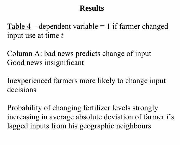
32

Results Table 4 – dependent variable = 1 if farmer changed input use at time t Column A: bad news predicts change of input Good news insignificant Inexperienced farmers more likely to change input decisions Probability of changing fertilizer levels strongly increasing in average absolute deviation of farmer i’s lagged inputs from his geographic neighbours

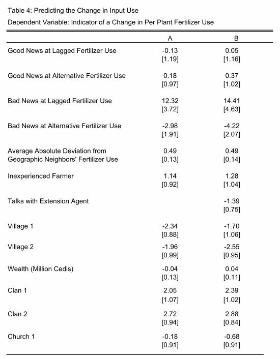
Table 4: Predicting the Change in Input Use

Dependent Variable: Indicator of a Change in Per Plant Fertilizer Use

Good News at Lagged Fertilizer Use -0.13 0.05[1.19] [1.16]

Good News at Alternative Fertilizer Use 0.18 0.37[0.97] [1.02]

Bad News at Lagged Fertilizer Use 12.32 14.41[3.72] [4.63]

Bad News at Alternative Fertilizer Use -2.98 -4.22[1.91] [2.07]

Average Absolute Deviation from 0.49 0.49Geographic Neighbors' Fertilizer Use [0.13] [0.14]

Inexperienced Farmer 1.14 1.28[0.92] [1.04]

Talks with Extension Agent -1.39[0.75]

Village 1 -2.34 -1.70[0.88] [1.06]

Village 2 -1.96 -2.55[0.99] [0.95]

Wealth (Million Cedis) -0.04 0.04[0.13] [0.11]

Clan 1 2.05 2.39[1.07] [1.02]

Clan 2 2.72 2.88[0.94] [0.84]

Church 1 -0.18 -0.68[0.91] [0.91]

BA

Logit MLE point estimates, spatial GMM (Conley 1999) standard errors in brackets allow for heteroskedasticity and correlation as a function of physical distance, see footnote 20 for details. Sample Size = 107. Pseudo R-squareds .34 and .36, columns A and B respectively. A full set of round dummies were included but not reported. Information neighborhoods defined using responses to: Have you ever gone to farmer ____ for advice about your farm?

34

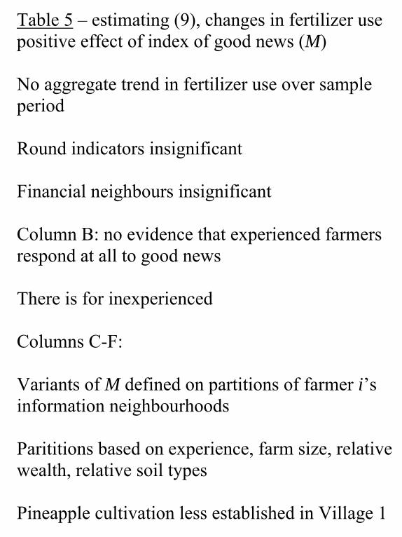
Table 5 – estimating (9), changes in fertilizer use positive effect of index of good news (M) No aggregate trend in fertilizer use over sample period Round indicators insignificant Financial neighbours insignificant Column B: no evidence that experienced farmers respond at all to good news There is for inexperienced Columns C-F: Variants of M defined on partitions of farmer i’s information neighbourhoods Parititions based on experience, farm size, relative wealth, relative soil types Pineapple cultivation less established in Village 1

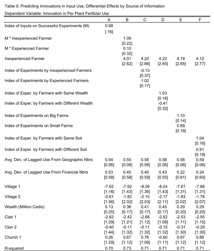
Table 5: Predicting Innovations in Input Use, Differential Effects by Source of Information

Dependent Variable: Innovation in Per Plant Fertilizer UseA

Index of Inputs on Successful Experiments (M) 0.99[.16]

M * Inexperienced Farmer 1.09[0.22]

M * Experienced Farmer 0.10[0.32]

Inexperienced Farmer 4.01 4.20 4.22 4.19 4.12[2.62] [2.66] [2.65] [2.65] [2.77]

Index of Experiments by Inexperienced Farmers -0.13[0.37]

Index of Experiments by Experienced Farmers 1.02[0.17]

Index of Exper. by Farmers with Same Wealth 1.03[0.18]

Index of Exper. by Farmers with Different Wealth -0.41[0.32]

Index of Experiments on Big Farms 1.10[0.14]

Index of Experiments on Small Farms 0.89[0.18]

Index of Exper. by Farmers with Same Soil 1.04[0.16]

Index of Exper. by Farmers with Different Soil 0.91[0.19]

Avg. Dev. of Lagged Use From Geographic Nbrs 0.54 0.55 0.58 0.58 0.58 0.59[0.06] [0.08] [0.06] [0.06] [0.06] [0.06]

Avg. Dev. of Lagged Use From Financial Nbrs 0.53 0.45 0.40 0.43 0.22 0.24[0.58] [0.58] [0.59] [0.55] [0.61] [0.60]

Village 1 -7.62 -7.92 -8.09 -8.24 -7.81 -7.88[1.16] [1.43] [1.36] [1.43] [1.31] [1.31]

Village 2 -0.61 -1.82 -2.15 -2.17 -1.83 -1.78[1.56] [2.02] [2.03] [2.11] [2.02] [2.07]

Wealth (Million Cedis) 0.13 0.36 0.41 0.45 0.29 0.29[0.25] [0.17] [0.17] [0.17] [0.20] [0.20]

Clan 1 -2.62 -2.42 -2.68 -2.62 -2.53 -2.55[1.29] [1.21] [1.12] [1.09] [1.11] [1.15]

Clan 2 -0.40 -0.11 -0.11 -0.15 -0.31 -0.29[1.44] [1.32] [1.32] [1.32] [1.30] [1.30]

Church 1 0.26 0.67 0.76 -0.60 0.87 0.88[1.29] [1.12] [1.06] [1.11] [1.12] [1.12]

R-squared 0.70 0.73 0.71 0.71 0.71 0.71OLS point estimates, spatial GMM (Conley 1999) standard errors in brackets allow for heteroskedasticity and correlation as a function of physical distance, see footnote 20 for details. Sample Size = 107. A full set of round dummies included but not reported. Information neighborhoods defined using responses to: Have you ever gone to farmer ____ for advice about your farm?

FB C D E

36

Robustness Checks Table 6 – Check if finding that M predicts innovations in fertilizer is robust to changes in definition of an information link Column A: j named by i when asked open-ended questions about who gave advice Column B: i and j listed anywhere in other’s roster of interactions with other sample members Column C: based on predicted probabilities of going to another farmer for advice (estimates of Table 2) Result robust for inexperienced farmers

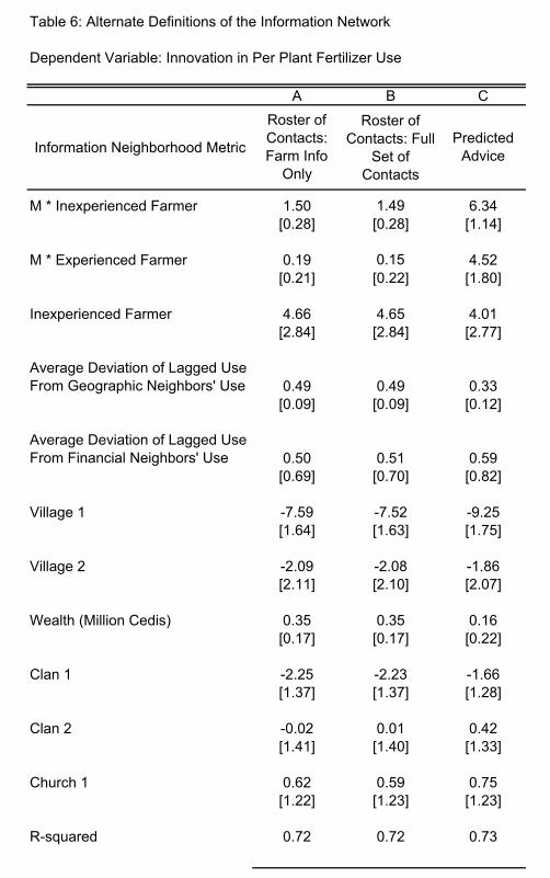
Table 6: Alternate Definitions of the Information Network

Dependent Variable: Innovation in Per Plant Fertilizer Use

B

Information Neighborhood Metric

Roster of Contacts: Full

Set of Contacts

M * Inexperienced Farmer 1.50 1.49 6.34[0.28] [0.28] [1.14]

M * Experienced Farmer 0.19 0.15 4.52[0.21] [0.22] [1.80]

Inexperienced Farmer 4.66 4.65 4.01[2.84] [2.84] [2.77]

Average Deviation of Lagged Use From Geographic Neighbors' Use 0.49 0.49 0.33

[0.09] [0.09] [0.12]

Average Deviation of Lagged Use From Financial Neighbors' Use 0.50 0.51 0.59

[0.69] [0.70] [0.82]

Village 1 -7.59 -7.52 -9.25[1.64] [1.63] [1.75]

Village 2 -2.09 -2.08 -1.86[2.11] [2.10] [2.07]

Wealth (Million Cedis) 0.35 0.35 0.16[0.17] [0.17] [0.22]

Clan 1 -2.25 -2.23 -1.66[1.37] [1.37] [1.28]

Clan 2 -0.02 0.01 0.42[1.41] [1.40] [1.33]

Church 1 0.62 0.59 0.75[1.22] [1.23] [1.23]

R-squared 0.72 0.72 0.73

OLS point estimates, spatial GMM (Conley 1999) standard errors in brackets allow for heteroskedasticity and correlation as a function of physical distance, see footnote 20 for details. Sample Size = 107. A full set of round dummies were included but not reported. Alternative information neighborhoods are as defined in Section 3.2 and Appendix 2.

CRoster of Contacts: Farm Info

Only

Predicted Advice

A

38

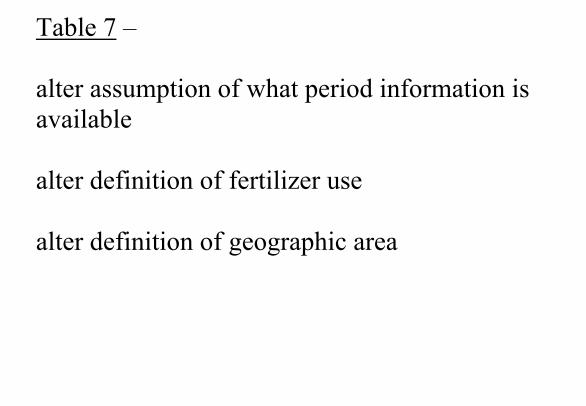
Table 7 – alter assumption of what period information is available alter definition of fertilizer use alter definition of geographic area

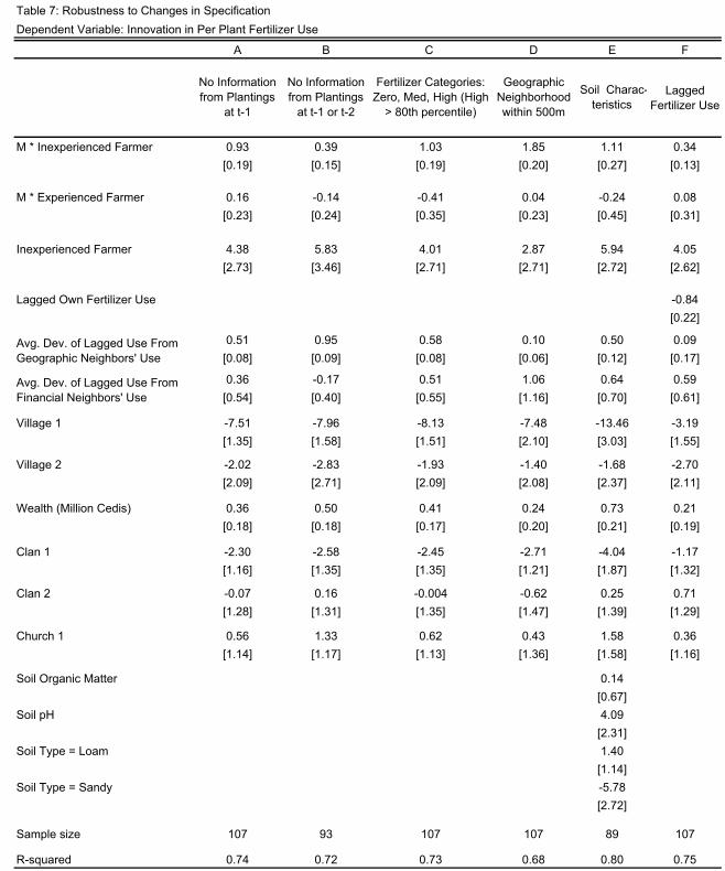
Table 7: Robustness to Changes in SpecificationDependent Variable: Innovation in Per Plant Fertilizer Use

F

Lagged Fertilizer Use

M * Inexperienced Farmer 0.93 0.39 1.03 1.85 1.11 0.34[0.19] [0.15] [0.19] [0.20] [0.27] [0.13]

M * Experienced Farmer 0.16 -0.14 -0.41 0.04 -0.24 0.08[0.23] [0.24] [0.35] [0.23] [0.45] [0.31]

Inexperienced Farmer 4.38 5.83 4.01 2.87 5.94 4.05[2.73] [3.46] [2.71] [2.71] [2.72] [2.62]

Lagged Own Fertilizer Use -0.84[0.22]

0.51 0.95 0.58 0.10 0.50 0.09[0.08] [0.09] [0.08] [0.06] [0.12] [0.17]

0.36 -0.17 0.51 1.06 0.64 0.59[0.54] [0.40] [0.55] [1.16] [0.70] [0.61]

Village 1 -7.51 -7.96 -8.13 -7.48 -13.46 -3.19[1.35] [1.58] [1.51] [2.10] [3.03] [1.55]

Village 2 -2.02 -2.83 -1.93 -1.40 -1.68 -2.70[2.09] [2.71] [2.09] [2.08] [2.37] [2.11]

Wealth (Million Cedis) 0.36 0.50 0.41 0.24 0.73 0.21[0.18] [0.18] [0.17] [0.20] [0.21] [0.19]

Clan 1 -2.30 -2.58 -2.45 -2.71 -4.04 -1.17[1.16] [1.35] [1.35] [1.21] [1.87] [1.32]

Clan 2 -0.07 0.16 -0.004 -0.62 0.25 0.71[1.28] [1.31] [1.35] [1.47] [1.39] [1.29]

Church 1 0.56 1.33 0.62 0.43 1.58 0.36[1.14] [1.17] [1.13] [1.36] [1.58] [1.16]

Soil Organic Matter 0.14[0.67]

Soil pH 4.09[2.31]

Soil Type = Loam 1.40[1.14]

Soil Type = Sandy -5.78[2.72]

Sample size 107

R-squared 0.74 0.72 0.73 0.68 0.80 0.75

Avg. Dev. of Lagged Use From Geographic Neighbors' Use

Avg. Dev. of Lagged Use From Financial Neighbors' Use

A B

No Information from Plantings

at t-1

Soil Charac-teristics

C

No Information from Plantings

at t-1 or t-2

Fertilizer Categories: Zero, Med, High (High

> 80th percentile)

Geographic Neighborhood within 500m

D E

OLS point estimates, spatial GMM (Conley 1999) standard. errors in brackets allow for heteroskedasticity and correlation as a function of physical distance, see footnote 20. Round dummies included but not reported. Alternative specifications are as defined in Section 6.2.

107 89107 93 107

40

Conclusion Evidence that social learning is important in diffusion of knowledge regarding pineapple cultivation in Ghana Take advantage of data to identify learning effects in economy undergoing rapid technological change Farmers more likely to change input levels of fertilizer use on receipt of bad news about profitability of their previous level of fertilizer use Less likely to change when observe bad news about profitability of alternative levels of fertilizer Magnitudes of innovations in fertilizer use: Farmer increases (decreases) his use after someone with whom he shares information achieves higher than expected profits when using more (less) fertilizer than he did

41

Findings hold when controlling for common input usage due to similar observable growing conditions

via conditioning on actions of geographic neighbours, credit arrangements, other info.

Support for interpretation as learning effect: inexperienced farmers are most responsive Information therefore has value as do the network connections through which information flows