Embed Size (px)
Citation preview
1/56
Instructor Tao, Wen-Quan
Key Laboratory of Thermo-Fluid Science & EngineeringInt. Joint Research Laboratory of Thermal Science & Engineering
Xi’an Jiaotong UniversityXi’an, 2018-Sept-17
Numerical Heat Transfer(数值传热学)
Chapter 3 Numerical Methods for Solving Diffusion Equation and their Applications (1)

2/56
3.1 1-D Heat Conduction Equation
3.2 Fully Implicit Scheme of Multi-dimensional
Heat Conduction Equation
3.3 Treatments of Source Term and B.C.
Contents
3.4 TDMA & ADI Methods for Solving ABEs
3.6 Fully Developed HT in Rectangle Ducts
3.5 Fully Developed HT in Circular Tubes
3/56
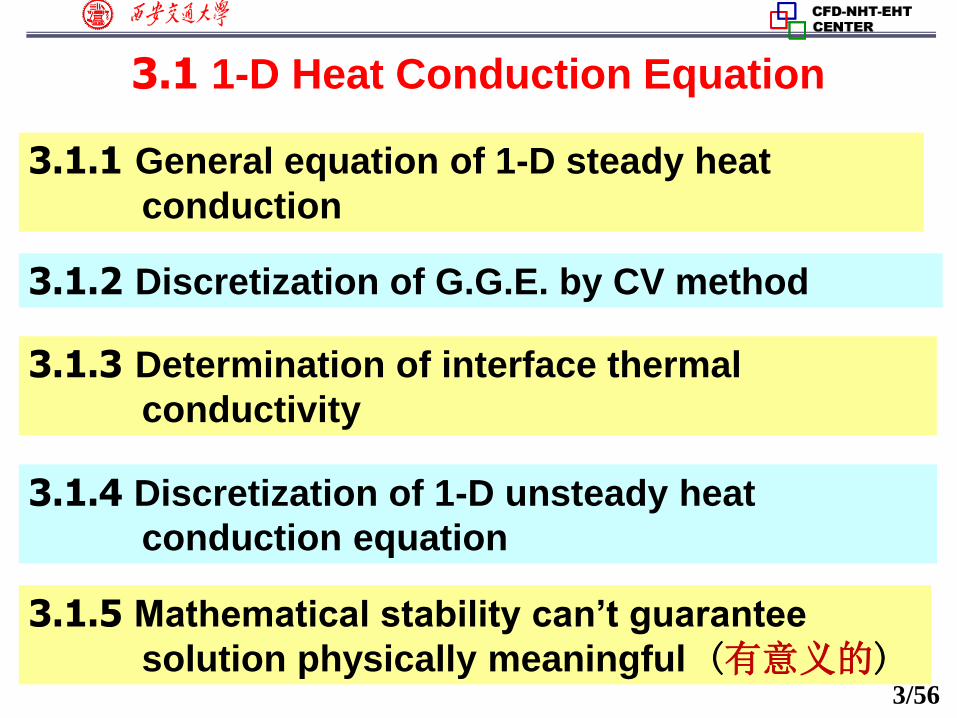
3.1 1-D Heat Conduction Equation
3.1.1 General equation of 1-D steady heat
conduction
3.1.3 Determination of interface thermal
conductivity
3.1.4 Discretization of 1-D unsteady heat
conduction equation
3.1.2 Discretization of G.G.E. by CV method
3.1.5 Mathematical stability can’t guarantee
solution physically meaningful (有意义的)

4/56
3.1 1-D Heat Conduction Equation
1. Two ways of coding for solving engineering problems
Special code(专用程序): FLOWTHERN,POLYFLOW……Having some generality within its
application range.
Different codes tempt to have some generality.
Generality includes:Coordinates;G.E.;B.C.
treatment;Source term treatment;Geometry……
General code(通用程序): HT, FF, Combustion,
MT, Reaction,etc.;PHOENICS,FLUENT,STAR-
CD ,CFX….
3.1.1 G.E. of 1-D steady heat conduction

5/56
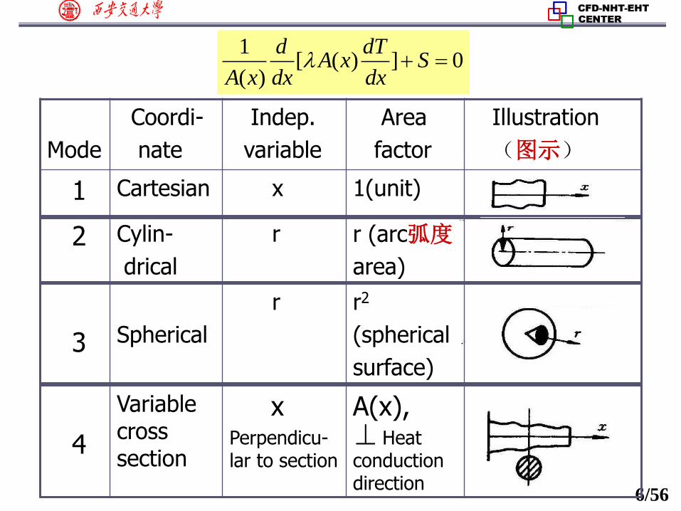
2. General governing equations of 1-D steady heat conduction problem
1[ ( ) ] 0
( )
d dTA x S
A x dx dx
x----Independent space variable (独立空间变量),
normal to cross section
A(x)----Area factor, normal to heat conduction
direction
----Thermal conductivity
S---- Source term, may be a function of both x and T.
6/56
Mode
Coordi-
nate
Indep.
variable
Area
factor
Illustration
(图示)
1 Cartesian x 1(unit)
2 Cylin-
drical
r r (arc弧度
area)
3 Spherical
r r2
(spherical
surface)
4
Variable cross section
xPerpendicu-lar to section
A(x), Heat
conduction direction
1[ ( ) ] 0
( )
d dTA x S
A x dx dx

7/56
3.1.2 Discretization of G.G.Eq. by CVM
[ ( ) ] ( ) 0d dT
A x S A xdx dx
Multiplying two sides by ( )A x
Linearizing (线性化) source term :C P PS S S T
Adopting piecewise linear profile:
[ ( ) ] [ ( ) ] ( ) ( ) 0e w C P P
dT dTA x A x S S T A x dx
dx dx
Integrating over control volume P
1[ ( ) ] 0
( )
d dTA x S
A x dx dx
yielding(得)
Sc and SP are constant in the CV.
8/56
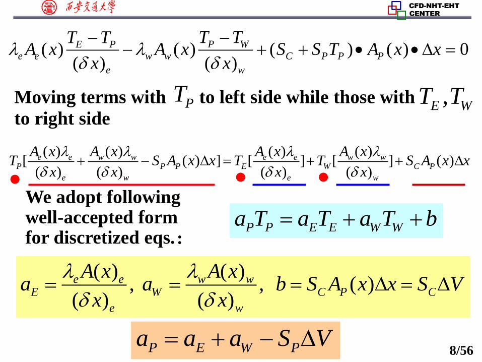
( ) ( ) ( ) ( ) 0( ) ( )
P WE P
e e w w C P P P
e w
T TT TA x A x S S T A x x
x x
Moving terms with to left side while those with
to right sidePT ,E WT T
( ) ( ) ( ) ( )[ ( ) ] [ ] [ ] ( )
( ) ( ) ( ) ( )
e e w w e e w wP P P E W C P
e w e w
A x A x A x A xT S A x x T T S A x x
x x x x
We adopt following well-accepted formfor discretized eqs.:
P P E E W Wa T a T a T b
( ) ( ), , ( )
( ) ( )
e e w wE W C P C
e w
A x A xa a b S A x x S V
x x
P E W Pa a a S V
9/56
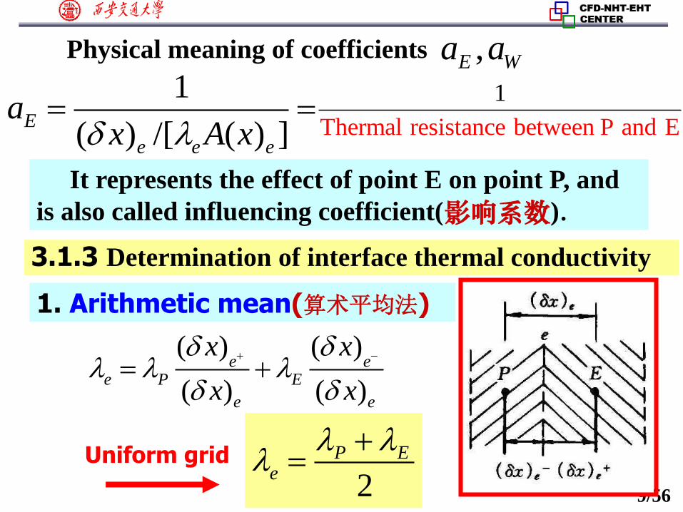
3.1.3 Determination of interface thermal conductivity
Physical meaning of coefficients ,E Wa a1
( ) /[ ( ) ]E
e e e
ax A x
Thermal resistance betwe
1
en P and E
It represents the effect of point E on point P, and
is also called influencing coefficient(影响系数).
1. Arithmetic mean(算术平均法)
( ) ( )
( ) ( )
e ee P E
e e
x x
x x
Uniform grid
2
P Ee

10/56
Right side
2. Harmonic mean(调和平均法)
Assuming that conductivities of P,E are different, according to the continuum requirement of heat flux (热流密度的连续性要求) at interface e
( ) ( )E e e P
e e
E P
T T T T
x x
( ) ( ) ( )E P E P
ee e
eE P
T T T T
x x x
Algebraic operation rule
Left side
Interface conductivity
( ) ( )( )e e e
e E P
x xx
( ) ( )E P
e e
E P
T T
x x
Harmonic mean
11/56
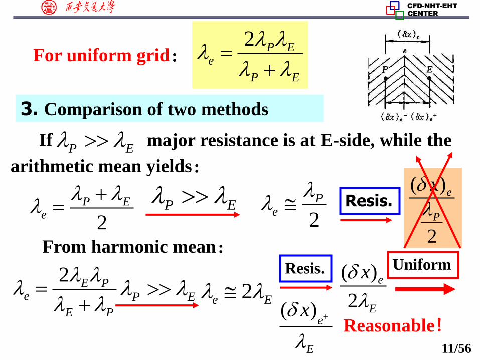
3. Comparison of two methods
IfP E major resistance is at E-side, while the
For uniform grid:2 P E
e
P E
2
P Ee
2
Pe
( )
2
e
P
x
Resis.
From harmonic mean:
2 E Pe
E P
2e E
Resis. ( )
2
e
E
x
Reasonable!
P E
P E ( )
e
E
x
Uniform
arithmetic mean yields:
12/56
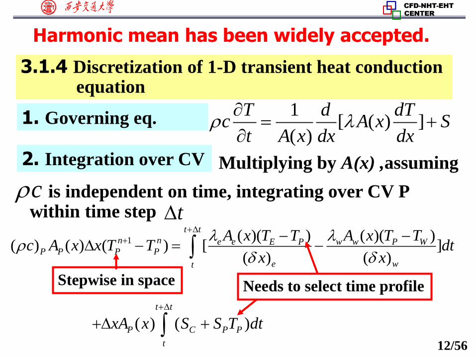
2. Integration over CV
Harmonic mean has been widely accepted.
3.1.4 Discretization of 1-D transient heat conductionequation
1[ ( ) ]
( )
T d dTc A x S
t A x dx dx
1. Governing eq.
tis independent on time, integrating over CV P
within time stepc
1 ( )( ) ( )( )( ) ( ) ( ) [ ]
( ) ( )
t t
n n e e E P w w P WP P P P
e wt
A x T T A x T Tc A x x T T dt
x x
( ) ( )
t t
P C P P
t
xA x S S T dt
Needs to select time profileStepwise in space
Multiplying by A(x) ,assuming
13/56
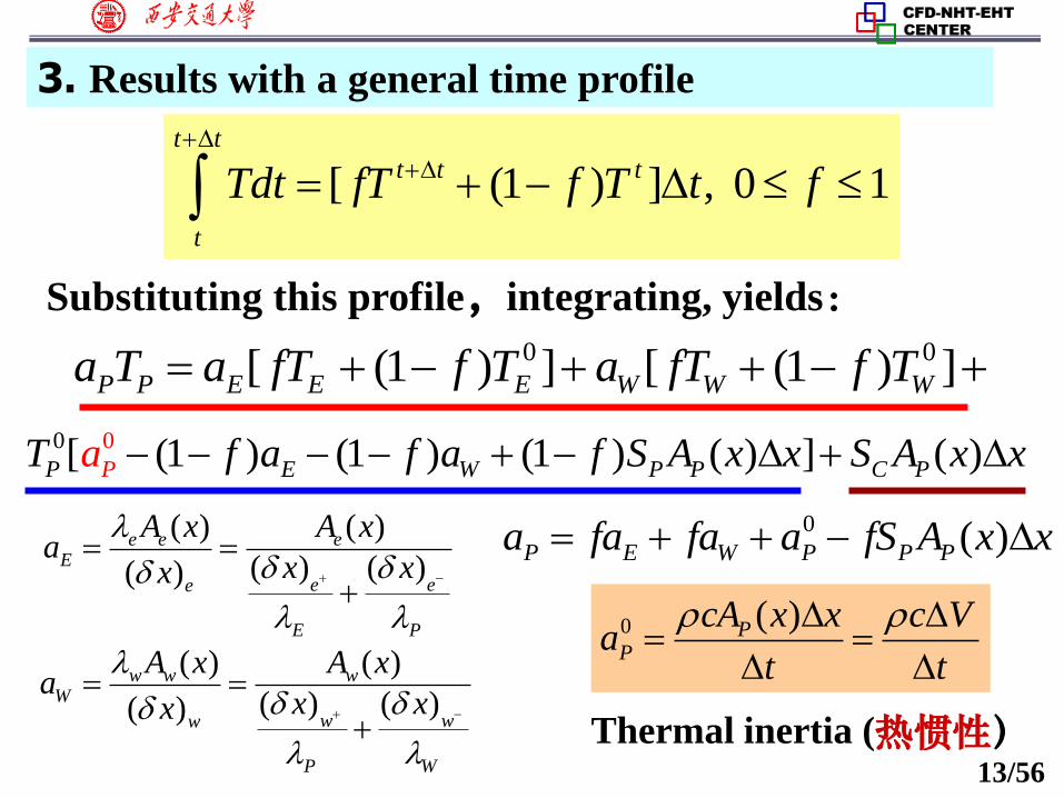
3. Results with a general time profile
[ (1 ) ] , 0 1
t t
t t t
t
Tdt fT f T t f
Substituting this profile,integrating, yields:0 0[ (1 ) ] [ (1 ) ]P P E E E W W Wa T a fT f T a fT f T
00[ (1 ) (1 ) (1 ) ( ) ] ( )P P E W P P C PT f a f a f S A x x S Aa x x
( ) ( )
( ) ( )( )
e e eE
e ee
E P
A x A xa
x xx
( ) ( )
( ) ( )( )
w w wW
w ww
P W
A x A xa
x xx
0 ( )P E W P P Pa fa fa a fS A x x
0 ( )PP
cA x x c Va
t t
Thermal inertia (热惯性)

14/56
4. Three forms of time level for discretized diffusion
term
(1) Explicit(显), 0 ;f
(2) Fully implicit(全隐), 1 ;f
0 0 0 0
2 2
2 2( )
2
P P E P W E P WT T a T T T T T T
t x x
(3)C-N scheme, 0.5f
0 0 00
2
2( )E P WP PT T TT T
at x
0
2
2( )E P WP PT T TT T
at x
No subscript for ( ) time levelt t
15/56
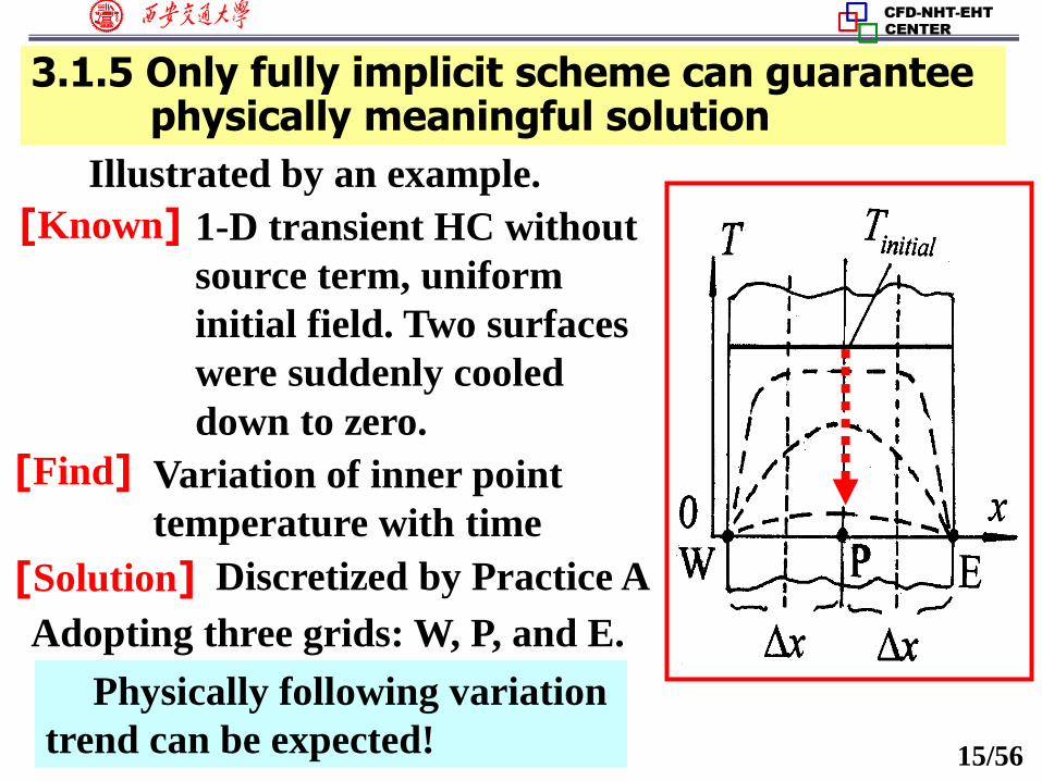
3.1.5 Only fully implicit scheme can guaranteephysically meaningful solution
Illustrated by an example.
1-D transient HC without
source term, uniform
initial field. Two surfaces
were suddenly cooled
down to zero.
[Known]
Variation of inner point
temperature with time
[Find]
Discretized by Practice A[Solution]
Adopting three grids: W, P, and E.
Physically following variation
trend can be expected!

16/56
Analyzing the 2nd time level:0 0 0 ;E E W WT T T T
Yields 0 0[ (1 ) (1 ) ]P P E WPPa T T f a f aa
0, 0C PS S
i.e.:0 0
0 0
(1 )( ) (1 )( )
( )
P P W E P W E
P P P W E
T a f a a a f a a
T a a f a a
1,E Wa a
x
0 ,p
P
c xa
t
Finally:0
2
2
1 2(1 )( )
1 2 ( )
P
P
a t
xa
fT
T t
xf
0 2 2
/( )
/
E
P p p
a x t a t
a c x t c x x
0 0[ (1 ) ] [ (1 ) ]P P E E E W W Wa T a fT f T a fT f T
00[ (1 ) (1 ) (1 ) ( ) ] ( )P P E W P P C PT f a f a f S A x x S Aa x x
Substituting:
0 0 0 0
0 0
2
a tFo
x

17/56
0
1 2(1 )
1 2
P
P
T f Fo
T fFo
Physically it is
required :
00P
P
T
T
Only fully implicit scheme can guaranteepositive ratio
18/56
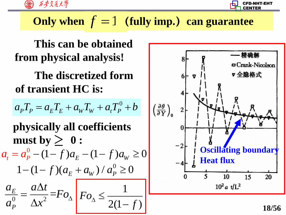
Only when 1f (fully imp.)can guarantee
This can be obtained
from physical analysis!
0
P P E E W W t Pa T a T a T aT b
0 (1 ) (1 ) 0EP Wt f a fa a a 01 (1 )( ) / 0E W Pf a a a
1
2(1 )Fo
f
physically all coefficients
must by 0 :
The discretized form
of transient HC is:
0 2=E
P
a a tFo
a x
Oscillating boundary
Heat flux
19/56
Conclusion:Only fully implicit scheme can guarantee
solution physically meaningful!
3.2 Fully Implicit Scheme of Multi-dimensional
Heat Conduction Equation
3.2.1 Fully implicit scheme in three coordinates
3.2.2 Comparison between coefficients
3.2.3 Uniform expression of discretized form for
three coordinates

20/56
3.2 Fully Implicit Scheme of Multi-dimensional Heat Conduction Equation
3.2.1 Fully implicit scheme in three coordinates
1. Cartesian coordinates
( ) ( )T T T
c St x x y y
(1)Governing eq.
(2)CV integration
Space profiles are the same as 1-D problem.
Heat flux is uniform at interface.Fully implicit for time

21/56
Integration of transient term=
n e t t
s w t
Tc dxdydt
t
stepwise 0( ) ( )P P Pc T T x y
Diffusion term(1)= ( )
n e t t
s w t
Tdxdydt
x x
[( ) ( ) ]
n t t
e w
s t
T Tdydt
x x
Space linear wise
Heat flux uniform,
Time fully implicit
( )( ) ( )
E P P We w
e w
T T T Ty t
x x
No subscript for
(n+1) time level=

22/56
Diffusion term (2)= ( )
n e t t
s w t
Tdxdydt
y y
[( ) ( ) ]
e t t
n s
w t
T Tdxdt
y y
Source term=
e n t t
w s t
Sdxdydt
( )C P PS S T x y t
Substituting and rearranging:
= ( )( ) ( )
N P P Sn s
n s
T T T Tx t
y y
Linealization
Fully implicit
Space linear wise
Heat flux uniform,
Time fully implicit
23/56
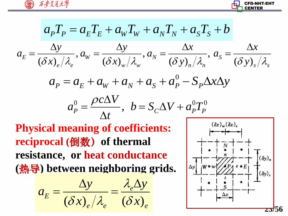
P P E E W W N N S Sa T a T a T a T a T b
, , ,( ) ( ) ( ) ( )
E W N S
e e w w n n s s
y y x xa a a a
x x y y
0
P E W N S P Pa a a a a a S x y
0 0 0,P C P P
c Va b S V a T
t
Physical meaning of coefficients:
reciprocal (倒数)of thermal
resistance, or heat conductance
(热导) between neighboring grids.
( ) ( )
eE
e e e
y ya
x x
24/56
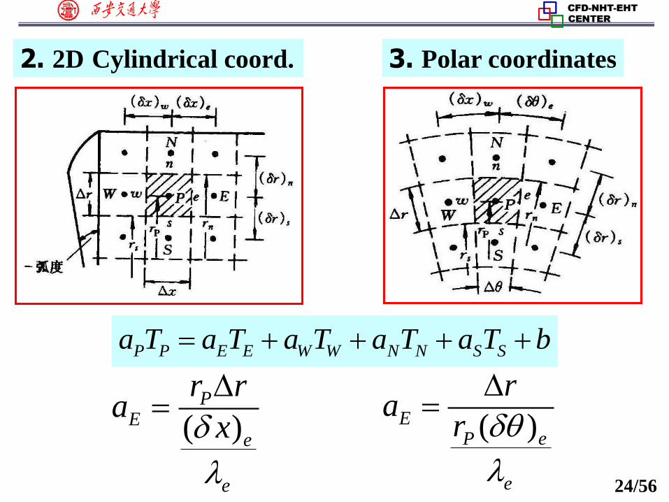
2. 2D Cylindrical coord. 3. Polar coordinates
P P E E W W N N S Sa T a T a T a T a T b
( )P
Ee
e
r ra
x
( )EP e
e
ra
r

25/56
3.2.2 Comparison between coefficients
Coefficients of the three 2-D coordinates can
be expressed as Ea
1.What’s the difference between 3 coordinates
(1)In polar coordi. is the arc (弧度), dimensionless,
(2)In polar and cylindrical coordinates there are radius,
while in Cartesian coordinate no any radius at all.
,x y x r ,while in
Ea Interface conductivity
Distance between Nodes E and P
E-W HC area
It is the thermal conductance between nodes E,P!
x is dimensional!

26/56
2. One way to unify the expression of coefficients
For this purpose we introduce two auxiliary (辅助的)
parameters
(1)Scaling factor in x –direction (x –方向标尺因子)
Distance in x direction is expressed by sx xFor Cartesian and cylindrical coordinates: 1;sx
(2)In y-direction, a normal(名义上的) radius, R, is
introduced.
Then: E-W conduction distance: sx xE-W conduction area: R /y sx
For polar coordinate: ;sx r
For Cy. & Po. R= rFor Cartesian coordi. R=1

27/56
Coordinate Cartes. Cy.Sym Polar Generalized
3.2.3 Unified expressions for three 2-D coordinates
E-W Coord. x x S-N Coord. y r r Y
Radius 1 r r R
Scaling factor in x
1 1 r SX
E-W distance
S-N distance ry r YE-W Conduct.area
y r r r /R Y SX
x x r ( )( )x SX
X

28/56
S-N Conuct.area
x r x r ( )R X
Volume of
CVr x r r r x y R X Y
Ea( ) /e e
y
x
( ) /e e
r r
x
( ) /e e
r
r
2( ) ( ) /e e
R Y
SX X
Na( ) /n n
x
y
( ) /n n
r x
r
( ) /n n
r
r
( ) /n n
R X
Y
0
Pa /cR X Y t
bcS R X Y

29/56
If coding by this way, then by setting up a
variable, MODE, computer will automatically deal
with the three coordinates according to MODE:
MODE 1(x-y) 2(x-r) 3(theta-r)
R
sx
1 r r
1 1 r
Commercial software usually adopts the
similar method to deal with coefficients in
different coordinates.
In our teaching code, it is set up as follows:

30/56
Brief review of 2018-09-17 lecture key points
1. 1-D G. G. Eq. for steady HC and its discretization
1[ ( ) ] 0
( )
d dTA x S
A x dx dx
P P E E W Wa T a T a T b
( ) ( ), , ( )
( ) ( )
e e w wE W C P C
e w
A x A xa a b S A x x S V
x x
P E W Pa a a S V
1
( ) /[ ( ) ]E
e e e
ax A x
Thermal resistance betwe
1
en P and E
= Conductance between P and E, influencing factor of E on P
31/56
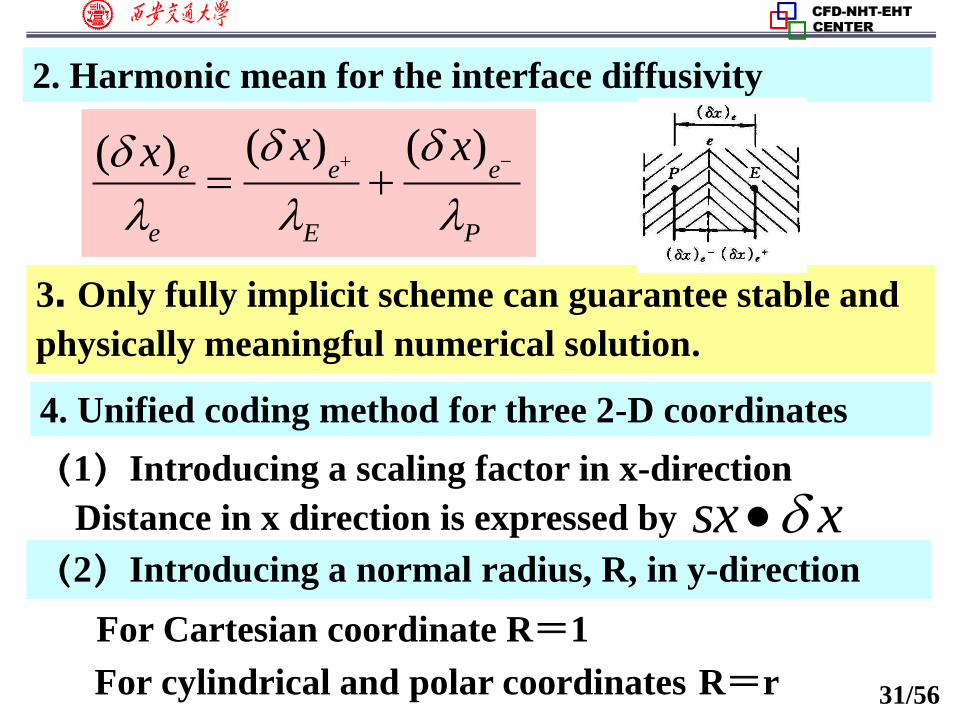
2. Harmonic mean for the interface diffusivity
3. Only fully implicit scheme can guarantee stable and
physically meaningful numerical solution.
( ) ( )( )e e e
e E P
x xx
4. Unified coding method for three 2-D coordinates
(1)Introducing a scaling factor in x-direction
Distance in x direction is expressed by sx x(2)Introducing a normal radius, R, in y-direction
For cylindrical and polar coordinates R=r
For Cartesian coordinate R=1

32/56
3.3 Treatments of Source Term and B.C.
3.3.1 Linearization of non-constant source term
1. Linearization (线性化) method
3.3.2 Treatments of 2nd and 3rd kind of B.C.
for closing algebraic equations
2. Discussion
3. Examples of linearization method
1. Supplementing(补充) equations for
boundary points
2. Additional source term method (ASTM)

33/56
3.3 Treatments of Source Term and B.C.
3.3.1 Linearization of non-constant source term
1. Linearization(线性化)
Importance of source term in the present method-
---”Ministry of portfolio (不管部长)”: refer to (指) any
terms which can not be classified as one of the
transient, diffusion or convection terms.
, 0C P P PS S S S
are constants for each CV,,C PS S
Linearization:for CV P its source term is expressed as:
is the slope(斜率) PS
curve ( )S f of the

35/56
2. Discussion on linearization of source term
(2)Any complicated function can be approximated by
a linear function, and linearity is also required by
deriving linear algebraic equations.
(3) is required by the convergence condition0PS
(1)For variable source term , , linearization
is better than taking previous value, .*( )PS f T
( )S f T
There is one time step lag (迟后) between
PC PTS S S and *( ) .S f T
for solving the algebraic equations.

36/56
P P nb nba a b
P nba a
P nb Pa a S V
The sufficient condition for obtaining converged
solution by iterative method for the algebraic equations
like:
is that:
Thus 0PS will ensure(确保) the above sufficient
Since in our method:
condition.
37/56
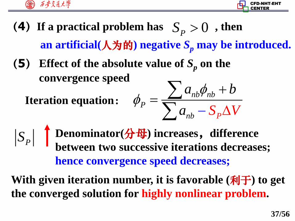
(4)If a practical problem has , then 0PS
(5) Effect of the absolute value of Sp on the
convergence speed
n
P
P
b nb
nb
a b
S Va
Iteration equation:
PS Denominator(分母) increases,difference
between two successive iterations decreases;
hence convergence speed decreases;
an artificial(人为的) negative Sp may be introduced.
With given iteration number, it is favorable (利于) to get
the converged solution for highly nonlinear problem.

38/56
Curve 1--normal ;Curve 3-- Absolute value of SP increases-It is in favor
of getting a converged solution for nonlinear case, while
speed of convergence decreases.
Curve 2 --Absolute value of SP decreases, it is in favor of
speed up iteration, but takes a risk(风险) of divergence!

39/56
3. Examples of linearization
(1) 3 5 ;S T
(2)
3, 5C PS S
Different
practices:
3 5 ;S T *3 5 , 0C PS T S
*3 7 , 2C PS T S
…………….
(3) 24 2 ;S T
* * * * 2( ) ( ) [4 (2 ) ]dS
S S T T TdT
* *( 4 )( )T T T
2*2 *2 * * *4 2 4 4 4 2 4T T T T T T T
CS PSRecommended
40/56
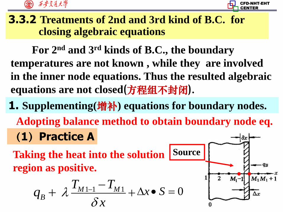
3.3.2 Treatments of 2nd and 3rd kind of B.C. for closing algebraic equations
1. Supplementing(增补) equations for boundary nodes.
For 2nd and 3rd kinds of B.C., the boundary
temperatures are not known , while they are involved
in the inner node equations. Thus the resulted algebraic
equations are not closed(方程组不封闭).
Adopting balance method to obtain boundary node eq.
(1)Practice A
Taking the heat into the solution
region as positive.
Bq 1 1 1M MT T
x
0x S
Source

41/56
Yields:1 1 1M MT T
x x S
Bq x
2( )O xThe T.E. of this discretized equation is:
(2)Practice B
For 3rd kind B.C., according to Newton’s law of cooling:
Substituting qB into the above equation, and rearranging:
1 1
1
( )
1
M f
M
x x S h xT T
Th x
1( )B f Mq h T T (Heat into the region as )

42/56
The volume of boundary node in Practice B is zero,
thus setting zero volume of the boundary nodes in the
above equation:
for 2nd kind
boundary-1 1 1
BM M
q xT T
for 3rd kind
boundary-
1 1
1
( )
1
M f
M
h xT T
Th x
The above discretized forms have 2nd order accuracy.
Bq 1 1 1M MT T
x
0x S
Zero boundary CV
0
yields:

43/56
(3)Example 4-4
[Known]2
20; 0, 0; 1, 1
d T dTT x T x
dx dx
[Find] Temperatures of 2-3 nodes in the region
[Solution]
Practice A,2 inner nodes,
2 3,T T Adopting 2nd–order accuracy discretization eq.
4T Adopting 1st order :4 3 11/3
T T 4 3 1/3T T
4T Adopting 2nd order: 1 1 1M MT T x x S
Bq x

44/56
Question 1:what is the source term?
4S T From 2
20
d TT
dx
We have4
1 1 11
3 6 34 31 1
T
T T
4 3
19 1
18 3T T
Effect of order of accuracy of B.C.on the numerical solution
Scheme T2 T3 T4
Analytical 0.2200 0.4648 0.7616
First order 0.2477 0.5229 0.8563
2nd order 0.2164 0.4570 0.7408
Then from
Question 2:what is the boundary heat flux?
1 1 1dT
qdx
1 1 1M MT T x x S
Bq x

45/56
Practice B,three CVs,
three inner nodes
1 1 1B
M M
q xT T
can be calculated from
For inner nodes adopting 2nd order;2 3 4, ,T T T
5T
Numerical results are much closer to exact solution!
Question:How to get the discretized eqs. for 2,4 ?
Scheme T2 T3 T4 T5
Exact 0.1085 0.3377 0.6408 0.7616
Practice B 0.1084 0.3372 0.6035 0.7702

46/56
2. Additional source term method (ASTM 附加源项法)
(1)Basic idea
Regarding the heat going into the region by 2nd or 3rd
kind B.C. as the source term of the first inner CV;
Cutting the connection between inner node and
boundary, i,e, regarding the boundary as adiabatic,
hence eliminating (消除)the
wall temp. from discretized
eqs. of inner nodes.
(2)Analysis for 2nd kind B.C.
P P E E W W
N N S S
a T a T a T
a T a T b

47/56
.( )
BW
B
ya
x
where Subtracting W Pa T
( )P W Pa a T ( )E E N N S S W W Pa T T a Ta T Ta b
( )W W Pa T T ( )
( )
B W P
B
T Ty
x
Bq y (entering as + )
'
P P E E N N S S CBq
a T a T a T a TV
S Vy
V
,C adS'
P P Wa a a
Summary of ASTM for 2nd kind B.C.:
from above eq.

48/56
(1)Adding a source term in discretized eq.
(2)Setting the conductivity of boundary node to be zero,
0Wa
(3)Discretizing inner nodes as usual.
(3)Analysis for 3rd kind B.C.
( )B f Wq h T T (Entering as + )
1 ( ) 1 ( )f W W P
BB
B B
P
B
fT TT T T
qx x
h h
T
Substituting the result to
the source term for 2nd
kind B.C.,
,B
C ad
q yS
V
, fh T
leading to:
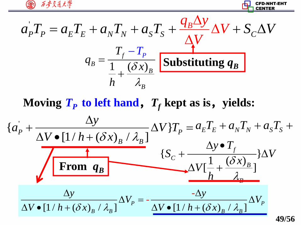
49/56
'{ }[1/ ( ) / ]
P P
B B
ya V T
V h x
1 ( )f
BB
B
PT
qx
h
T
E E N N S Sa T a T a T
{ }1 ( )
[ ]
f
CB
B
y TS V
xV
h
'
P P E E N N S S CBq
a T a T a T a TV
S Vy
V
Substituting qB
Moving TP to left hand,Tf kept as is,yields:
From qB
--
[1 / ( ) / ] [1 / ( ) / ]P P
B B B B
y yV V
V h x V h x

50/56
,[1 / ( ) / ]
P ad
B B
yS
V h x
, 1 ( )[ ]
f
C adB
B
y TS
xV
h
(4)Implementing procedure of ASTM
Determining ASTs for CV neighboring to boundary, ,, ,C ad P adS S
,C C adS SCS Accumulative
addition (累加)
Adding them into source term of related CV
'( )P P Pa a S
51/56
Setting the conductivity of the boun. node to be zero;
Deriving the discretized eqs. of inner nodes as usual,
Solving the algebraic eqs. for inner nodes;
Using Newton’ law of cooling or Fourier eq. to get
the boundary temperatures from the converged
solution of inner nodes.
(5)Application examples of ASTM
In FVM when Practice B is adopted to discretize
space, the 2nd and 3rd kinds of B.C. can be treated by
ASTM, which can greatly accelerate(加速) the
solution process.
52/56
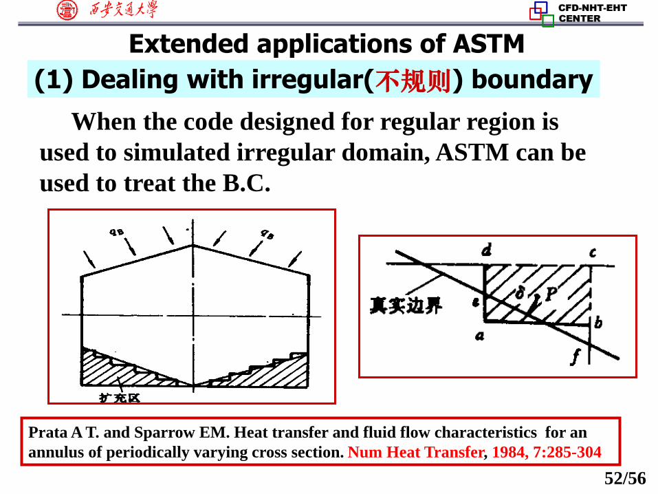
Extended applications of ASTM
When the code designed for regular region is
used to simulated irregular domain, ASTM can be
used to treat the B.C.
Prata A T. and Sparrow EM. Heat transfer and fluid flow characteristics for an
annulus of periodically varying cross section. Num Heat Transfer, 1984, 7:285-304
(1) Dealing with irregular(不规则) boundary

53/56
(2) Simulating combined conduction, convection and radiation problem
[1] 陶文铨,李芜.处理区域内部导热与辐射联合作用的数值方法. 西安交通大学学报,
1983,19(3):65-76
[2] 杨沫 王育清 傅燕弘 陶文铨. 家用冰箱冷冻冷藏室温度场的数值模拟. 制冷学报,
1991年,(4):1-8
[3] Zhao CY, Tao WQ. Natural convections in conjugated single and double
enclosures. Heat Mass Transfer, 1995, 30 (3): 175-182
54/56
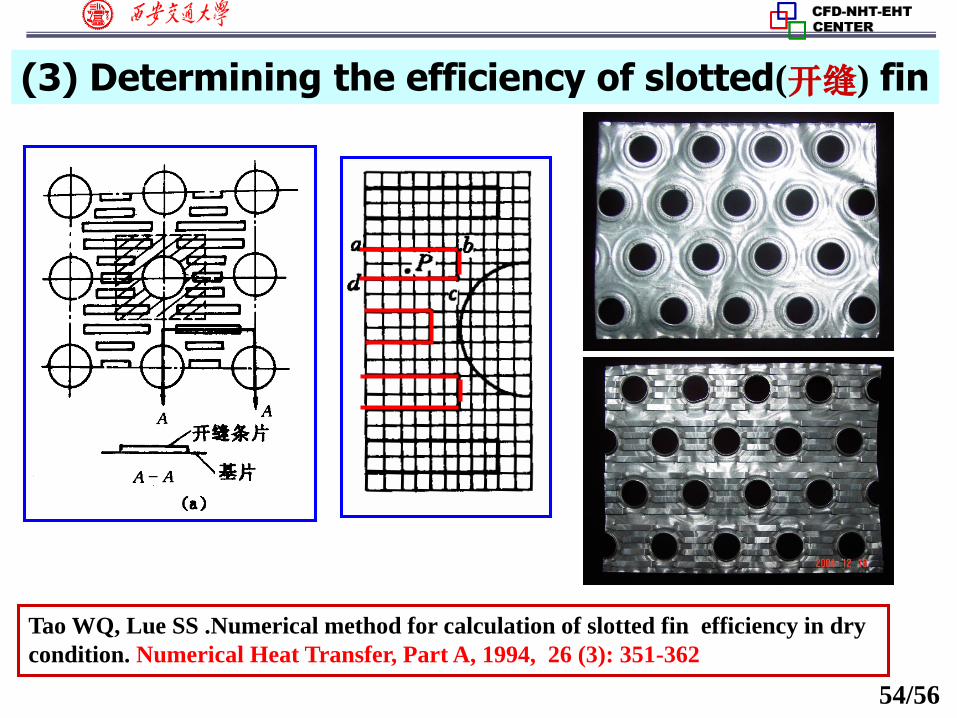
(3) Determining the efficiency of slotted(开缝) fin
Tao WQ, Lue SS .Numerical method for calculation of slotted fin efficiency in dry
condition. Numerical Heat Transfer, Part A, 1994, 26 (3): 351-362

55/56
(4) Simulating heat transfer and fluid flow in a welding pool (焊池)
Lei Y P,Shi Y W. Numerical treatment of the boundary conditions and source term
of a spot welding process with combining buoyancy – Marangoni flow. Numerical
Heat Transfer, Part b, 1994, 26 : 455-471


![Chapter 4 Numerical Solution of Diffusion Equation and its ...nht.xjtu.edu.cn/__local/A/0F/C4/A85917D9C4F0AD42EB...4.1.2 Discretization of G.G.Eq. by CVM [ ( ) ] ( ) 0 d dT A x S A](https://img.pdfslide.tips/doc/110x75/5e50942cbec88c5ae31d8608/chapter-4-numerical-solution-of-diffusion-equation-and-its-nhtxjtueducnlocala0fc4a85917d9c4f0ad42eb.jpg)