國立交通大學 - National Chiao Tung UniversityEach sensing node is controlled by an Imote2 platform comprised of a microprocessor, sensor module, and communication device. To

國立交通大學

土木工程學系

博士論文

整合式無線感測網路之結構健康監測系統

於建築與土木結構之研發

DEVELOPMENT OF AN INTEGRATED WIRELESS SENSOR

NETWORK-BASED STRUCTURAL HEALTH MONITORING

SYSTEM FOR BUILDINGS AND CIVIL

INFRASTRUCTURES

研究生:林子軒

指導教授: 洪士林博士

中華民國一百年六月




NETWORK-BASED STRUCTURAL HEALTH MONITORING

SYSTEM FOR BUILDINGS AND CIVIL INFRASTRUCTURES

研究生：林子軒 Student: Tzu-Hsuan Lin

指導教授：洪士林博士 Advisor: Dr. Shih-Lin Hung

國立交通大學

土木工程學系

博士論文

A Dissertation

Submitted to Department of Civil Engineering

College of Engineering

National Chiao Tung University

In partial Fulfillment of the Requirements

for the Degree of

Doctor of Philosophy

in

Civil Engineering

June 2011

Hsinchu, Taiwan, Republic of China

中華民國一百年六月

I



研究生：林子軒指導教授：洪士林博士

國立交通大學

土木工程學系

摘要

本研究提出一整合式無線感測網路之結構健康監測系統架構並應用於建築

與土木結構上。此架構主要包含了感測、資訊融合與管理以及決策診斷。在此架

構目標下，本研究發展了一個整合式無線感測網路結構健康監測系統。此系統由

多種無線節點所組成，包含感測結點、簇首節點、傳送節點與基地台。感測結點

主要以 Imote2 平台為基礎，用來量測結構的動態反應或是環境參數。簇首節點

為雙核心之設計結合了 Imote2 平台與額外之嵌入式系統。簇首節點含有額外之

無線通訊模組與 GPS來進行較長距離之資料接收、交換，並可以進行定位與同步

之用。傳送節點可當作協調者並進行資料的跳躍傳送(Hopping)。基地台主要為

接收所有回傳的感測資料與訊息，其硬體能力為所有結點中最高的。此系統亦包

含了一個三層式的軟體架構，主要可以進行可靠的資料感測與傳輸、資料儲存、

視覺化之使用者介面、資料分析與訊號處理等工作。在此軟體架構下，無線感測

相關的結構健康監測的應用將可以很容易地被實行。此外，能源的消耗亦是無線

感測的一個很重要的問題，因此，本研究發展了一個結合壓電、風車、與磁場的

整合式能源擷取系統來改善能源消耗的問題。結構健康監測可分為局部與全域

之方法，然而，兩種方法各有其優缺點與應用之時機。因此本研究發展了一個整

II

合式的結構損害評估方法整合全域與局部之結構損害評估法，應用於結構健康監

測上。在全域結構損害偵測方面，本文分別提出了新的子結構頻率響應函數法來

對結構進行大範圍之損害評估。接著，以電機阻抗為主之局部損害評估法則可以

用來進行小範圍局部損害之評估。

在實驗與數值模擬研究中，數值模擬的結果發現本文所提出之結構損壞評估

方法可以成功地找出結構發生損壞的位置。另外無線感測網路結構健康監測系統

亦於一縮尺之建築模型上進行驗證，其實驗結果證實此系統可進行高質量的感測

與資料傳輸並可以精確地獲得結構的相關動態反應參數。為驗證所發展之無線感

測網路結構健康監測系統應用於實際土木結構上之可行性，將此系統佈設於一橋

梁上進行驗證。實驗結果顯示，此系統於實際土木之結構上依然可以獲得相當好

的感測結果，無線傳輸也可以達到預期的效果。在實際土木結構監測的佈設上更

可以發現本系統之優點，在實驗過程中，平均一個節點的建置小於 5分鐘，比起

傳統有線的監測系統來說，在時間成本的節省上更顯現出本系統的優勢。在六層

樓縮尺模型試驗中，亦可以證實本研究所提出之整合式的結構損害評估方法可以

識別出結構之全域與局部之損害。

III


NETWORKS-BASED STRUCTURAL HEALTH MONITORING

SYSTEM FOR BUILDINGS AND CIVIL INFRASTRUCTURES

Student: Tzu-Hsuan Lin Advisor: Dr. Shih-Lin Hung

Department of Civil Engineering

College of Engineering

National Chiao Tung University

ABSTRACT

The main purpose of this dissertation was to propose a framework for an

integrated wireless sensor network (WSN)-based structural health monitoring (SHM)

system in buildings and civil infrastructures. In this framework, three main parts were

considered: the physical sensing; information fusion and management; and inference

and decision making. To achieve this goal, an integrated WSN-based SHM system

was developed. This system consists of sensing nodes, cluster head nodes, transfer

node, and base station. The sensing node measures structural response or

environmental parameters. Each sensing node is controlled by an Imote2 platform

comprised of a microprocessor, sensor module, and communication device. To

exchange information or to trigger sensing tasks, the cluster head node can

communicate with sensing nodes or cluster heads of neighboring communities. The

cluster head has a dual-core design that combines the Imote2 platform with a second

embedded device. The cluster head has an extra wireless module and GPS. The extra

wireless module provides additional RF power needed for long-range wireless

IV

communication. The GPS is useful for synchronization and localization. The transfer

node functions as a coordinating node for managing cluster heads and data hopping.

The base station is the highest level end device and has the largest memory, the most

powerful processor and the highest communication capability. The base station node

is the gateway between smart sensor networks and the Host computer.

A three-tier software framework is also developed in this work serving as reliable

data-sensing and transmission, data logging and data storage, user interface, data

analyzing, and signal processing. Based on this software framework, a SHM

application for specific purpose can be easily developed. Power sources and power

consumption are the critical issue in WSN if batteries have to be periodically replaced.

Hence, a novel windmill-magnet integrated piezoelectric (WMIP) energy harvesting

system was also proposed.

Since local and global SHM have unique benefits and shortcomings, an

integrated approach may be more effective than using either approach alone. This

work developed a global-local-integrated damage detection approach for localizing

damage. Substructure-based frequency response function approaches were proposed

for global damage detection. Local damage was then identified by

Electro-Mechanical-Impedance (EMI)-Based damage detection method.

Numerical and experimental study is also conducted to complete this study.

Numerical results reveal that the proposed global damage detection approach can

successfully locate damage at a single site and at multiple sites. Experimental analysis

confirms the proposed integrated WSN-based SHM system provides excellent data

sensing and transmission quality for determining the structural dynamic properties.

V

An experimental validation in building structure confirms that the proposed global

SHM approach can indicate the approximate location of the damaged area in damaged

floor and the EMI-based damage detection approach can check the component of

building structure locally. Subsequently, the proposed WSN-based SHM system is

employed in a bridge structure to test the feasibility in field. This experimental result

confirms good-quality data collection by the proposed system. In experimental period,

the system shows WSN-based SHM system outperforms conventional SHM system,

especially in deploying sensors. Average time for deploying single node only takes

within 5min.

VI

ACKNOWLEDGEMENT

時間飛逝，轉眼間在交大也待了六個年頭了，學生生涯也在此畫下了句點。讀

博士真是一個漫長的過程，其中辛酸只有經歷過的人才能夠體會吧。在博士期間，

受到許許多多的幫助，在此獻上我最深的感謝。

當然最要感謝的是我的指導教授洪士林博士，他在研究上給予我非常大的自由，

讓我可以進行我有興趣的研究，在論文的方向與內容給予我相當大的幫助，並在

在其身上學到一個研究學者該有的風範。在生活方面，洪老師的國科會計畫也幫

助了我減輕經濟上的壓力。感謝黃炯憲老師在我論文中很重要的理論部分給予我

相當大的指導，在黃老師的身上也學到做研究嚴謹的態度。感謝廖德誠老師在電

機領域相關的指導，讓我跨領域的學習能夠如此的順利。另外，在博士班期間很

感謝東京大學的 Fujino 與 Nagayama 教授給我機會，讓我到東京大學訪問兩個

月，這兩個月讓我學習到很多東西，是個難忘的經驗。感謝靜宜大學吳仁彰教授

帶領我進入跨領域的研究，也感謝其時時為我禱告。感謝 Murthy 博士，無論是

在研究或是 paper的撰寫都給予我相當大的幫助，在他身上也學到很多。感謝中

興工程科技研究發展基金會，中興工程顧問社，中華顧問工程司，給予我的獎學

金。讓我能夠專心於研究上，不用為經濟擔心。

感謝研究室同學勇奇在我研究上有問題時可以互相討論，感謝研究室學弟們在

我實驗上的幫忙，感謝一弘在我修習電機相關課程時給予我幫助，並在 WSN的領

域一起努力學習，感謝阿銘在天線上面的幫助，感謝秦飛在 Imote2 上給予的協

助。還有許多在我博士班期間幫助過我的朋友，無法在此一一列出，在這一起獻

上我的感謝。也要感謝女友珮茹這幾年來對我的鼓勵與關心。最後要感謝我的家

人，沒有你們的支持，我沒有辦法專心地完成我的博士學位，感謝我的母親，您

辛苦了。

VII

CONTENTS

摘要 ............................................................................................................................................ I

ABSTRACT.................................................................................................................................. III

ACKNOWLEDGEMENT ...............................................................................................................VI

CONTENTS ............................................................................................................................... VII

LIST OF TABLES .......................................................................................................................... XI

LIST OF FIGURES ....................................................................................................................... XII

CHAPHER 1 INTRODUCTION ....................................................................................................... 1

1.1 BACKGROUND OF STRUCTURAL HEALTH MONITORING .................................................................. 1

1.2 MOTIVATION AND OBJECTIVE ................................................................................................... 3

1.3 OVERVIEW OF DISSERTATION .................................................................................................... 7

CHAPHER 2 LITERATURE REVIEW .............................................................................................. 10

2.1 INTRODUCTION ................................................................................................................... 10

2.2 STRUCTURAL HEALTH MONITORING APPROACH ......................................................................... 10

2.2.1 Global Damage Detection Method ........................................................................ 10

2.2.2 Local Damage Detection Method .......................................................................... 13

2.3 WIRELESS SENSOR NETWORKS-BASED STRUCTURAL HEALTH MONITORING APPLICATIONS ................. 15

CHAPHER 3 WIRELESS SENSOR NETWORKS .............................................................................. 18

VIII

3.1 INTRODUCTION TO WIRELESS SENSOR NETWORKS (WSN)........................................................... 18

3.2 SUBSYSTEM OF SMART WIRELESS SENSOR NODE ....................................................................... 20

3.3 WIRELESS SENSOR PLATFORMS............................................................................................... 21

3.4 FACTORS INFLUENCING SENSOR NETWORK DESIGN .................................................................... 23

3.5 THE 802.15.4 AND ZIGBEE STANDARDS .................................................................................. 25

3.6 OPERATING SYSTEMS FOR WIRELESS SENSOR NETWORKS ............................................................ 29

3.7 TIME SYNCHRONIZATION ....................................................................................................... 34

CHAPHER 4 INTEGRATED WSN-BASED SHM SYSTEM ................................................................. 37

4.1 INTRODUCTION ................................................................................................................... 37

4.2 ARCHITECTURE OF INTEGRATED WSN SHM SYSTEM .................................................................. 38

4.3 HARDWARE DESIGN ............................................................................................................. 39

4.3.1 Sensing Node ......................................................................................................... 40

4.3.2 Cluster Head and Transfer Node ............................................................................ 44

4.3.3 Base Station........................................................................................................... 47

4.3.4 Multi-Sensor Board Design .................................................................................... 48

4.3.5 Power Module ....................................................................................................... 52

4.4 WINDMILL-MAGNET INTEGRATED PIEZOELECTRIC (WMIP) ENERGY HARVESTING SYSTEM................. 52

4.4.1 General Theory of Vibration-Based Energy Harvesting Method ........................... 53

4.4.2 Energy Harvesting Circuits .................................................................................... 54

IX

4.4.3 Windmill-Magnet Integrated Piezoelectric Energy Harvesting System ................. 57

4.5 THREE-TIER SOFTWARE FRAMEWORK ...................................................................................... 62

4.5.1 Net Micro Frameworks-Based Embedded Development Environment .................. 64

4.5.2 Data Logging and Data Storage ............................................................................ 68

4.5.3 User Interface and Visualized Signal Processing ................................................... 69

4.6 RELIABLE DATA-SENSING AND TRANSMISSION SERVICE ................................................................ 72

CHAPHER 5 DEVELOPMENT OF GLOBAL-LOCAL-INTEGRATED DAMAGE DETECTION APPROACH76

5.1 INTRODUCTION ................................................................................................................... 76

5.2 SUBSTRUCTURE-BASED FREQUENCY RESPONSE FUNCTION FOR GLOBAL DAMAGE DETECTION ............ 78

5.2.1 Substructure-Based Frequency Response Function Approach ............................... 80

5.2.2 Numerical Study .................................................................................................... 91

5.2.3 Implement of SubFRFDI in Integrated WSN-Based SHM System ......................... 111

5.3 ELECTRO-MECHANICAL-IMPEDANCE (EMI)-BASED LOCAL DAMAGE DETECTION METHOD ............... 114

5.3.1 Fundamental of EMI-Based Model ...................................................................... 114

5.3.2 Measurement of Piezoelectric-Impedance .......................................................... 117

5.3.3 Selection of Frequency Ranges ............................................................................ 118

CHAPHER 6 EXPERIMENTAL VERIFICATION ............................................................................. 120

6.1 INTRODUCTION ................................................................................................................. 120

6.2 VERIFICATION OF INTEGRATED WSN-BASED SHM SYSTEM ........................................................ 120

X

6.2.1 Verification of Sensing Node ............................................................................... 120

6.2.2 Reliability of RF Communication Test .................................................................. 127

6.2.3 Field Test in Bridge Structure ............................................................................... 130

6.2.3.1 Experimental Setup ............................................................................................. 132

6.2.3.2 Experimental Results ........................................................................................... 134

6.3 EXPERIMENTAL STUDY IN BUILDING STRUCTURE ....................................................................... 140

CHAPHER 7 CONCLUSIONS REMARKS ..................................................................................... 158

7.1 CONCLUSION .................................................................................................................... 158

7.2 FUTURE STUDY .................................................................................................................. 161

REFERENCE ............................................................................................................................. 163

VITA ........................................................................................................................................ 176

XI

LIST OF TABLES

TABLE 3.1 DESCRIPTION OF KEYWORDS IN TINYOS. ............................................................................................ 33

TABLE 4.1 COMPARISON OF MOTE PLATFORM ................................................................................................... 43

TABLE 4.2 SPECIFICATION OF XBEE MODELS. ..................................................................................................... 46

TABLE 4.3 PHYSICAL AND ELECTRICAL CHARACTERISTICS OF GYRO SENSOR ............................................................. 50

TABLE 4.4 PHYSICAL AND ELECTRICAL CHARACTERISTICS OF ACCELEROMETER SENSOR .............................................. 51

TABLE 4.5 DIFFERENT TYPES OF PIEZOELECTRIC PRODUCT .................................................................................... 58

TABLE 4.6 DESCRIPTION OF CLASS LIBRARY ....................................................................................................... 66

TABLE 4.7 TOSMSG HEADER CONTENTS ........................................................................................................... 68

TABLE 4.8 SENSOR BOARD HEADER CONTENT .................................................................................................... 69

TABLE 4.9 DATA PAYLOAD .............................................................................................................................. 69

TABLE 5.1 DESCRIPTIONS OF SIMULATED DAMAGE CASES. .................................................................................... 92

TABLE 6.1 DESCRIPTION DAMAGE SCENARIOS FOR THE STEEL-FRAME MODEL. ........................................................ 144

TABLE 6.2 COMPARISONS OF MODAL PARAMETERS IDENTIFIED BY WIRELESS SENSING NODES AND CONVENTIONAL

REFERENCE SENSORS. .................................................................................................................. 151

TABLE 6.3 THE PROCESSING TIME OF EMBEDDED FFT AND FRF FOR DIFFERENT DATA LENGTH. .................................. 152

XII

LIST OF FIGURES

FIGURE 1.1 THE RELATION BETWEEN USAGE MONITORING, STRUCTURAL HEALTH MONITORING, AND DAMAGE PROGNOSIS. 3

FIGURE 1.2 A FRAMEWORK OF AN INTEGRATED WIRELESS SENSOR NETWORK-BASED STRUCTURAL HEALTH MONITORING

SYSTEM. ................................................................................................................................... 7

FIGURE 3.1 COMPOSITION OF WIRELESS SENSOR NODE ....................................................................................... 21

FIGURE 3.2 802.15.4 AND ZIGBEE ARCHITECTURE ............................................................................................ 26

FIGURE 3.3. STAR TOPOLOGY ......................................................................................................................... 27

FIGURE 3.4. PEER-TO-PEER TOPOLOGY ............................................................................................................ 28

FIGURE 3.5 SCHEMA OF TINYOS (CROSSBOW) .................................................................................................. 30

FIGURE 3.6 ARCHITECTURE OF TINYOS ( CROSSBOW) ........................................................................................ 31

FIGURE 3.7 THE PROCESS IN TINYOS( CROSSBOW) ............................................................................................ 32

FIGURE 4.1 INTEGRATED WSN-BASED SHM SYSTEM ARCHITECTURE: DIFFERENT ROLES ARE ASSIGNED TO NODES .......... 39

FIGURE 4.2 PHOTO OF SENSING NODE ............................................................................................................. 40

FIGURE 4.3 BLOCK DIAGRAM OF SENSING NODE ARCHITECTURE. ........................................................................... 42

FIGURE 4.4 BLOCK DIAGRAM OF CLUSTER HEAD NODE ARCHITECTURE. .................................................................. 46

FIGURE 4.5 PHOTOGRAPH OF CLUSTER HEAD NODE ON BOX ................................................................................ 47

FIGURE 4.6 BLOCK DIAGRAM OF BASE STATION ARCHITECTURE.............................................................................. 48

FIGURE 4.7 SIMPLIFIED BLOCK DIAGRAM OF MULTI-SENSOR BOARD ..................................................................... 49

FIGURE 4.8 PHOTOGRAPHY OF DEVELOPED MULTI-SENSOR BOARD........................................................................ 50

XIII

FIGURE 4.9 (A) CANTILEVER BEAM WITH TIP MASS, (B) MODEL OF EQUIVALENT LUMPED SPRING MASS SYSTEM .............. 54

FIGURE 4.10 TYPICAL PIEZOELECTRIC HARVESTING CIRCUIT .................................................................................. 55

FIGURE 4.11 ARCHITECTURE OF ENERGY HARVESTING BASED WIRELESS SENSOR NODE ............................................... 57

FIGURE 4.12 SCHEMATIC DIAGRAM OF WINDMILL BASED PIEZOELECTRIC HARVESTING SYSTEM .................................... 58

FIGURE 4.13 EXPERIMENT SETUP OF WINDMILL BASED PIEZOELECTRIC HARVESTING SYSTEM: (A) RAW VOLTURE, (B)MFC,

(C)PZT, (D) OVERPASS IN TOKYO UNIVERSITY. ............................................................................... 59

FIGURE 4.14 OUTPUT VOLTAGE OF PZT ........................................................................................................... 60

FIGURE 4.15 OUTPUT VOLTAGE OF MFC ......................................................................................................... 60

FIGURE 4.16 OUTPUT VOLTAGE OF RAW VOLTURE ............................................................................................. 61

FIGURE 4.17 WINDMILL-MAGNET INTEGRATED PIEZOELECTRIC (WMIP) ENERGY HARVESTING SYSTEM ........................ 61

FIGURE 4.18 OUTPUT VOLTAGE AND FFT OF WMIP ENERGY HARVESTING SYSTEM .................................................. 62

FIGURE 4.19 THE PROPOSED SOFTWARE ARCHITECTURE ...................................................................................... 63

FIGURE 4.20 STRUCTURE OF CLASS LIBRARY ..................................................................................................... 65

FIGURE 4.21. PACKET FORMAT ....................................................................................................................... 68

FIGURE 4.22 FUNCTIONS OF PROPOSED USER INTERFACE .................................................................................... 70

FIGURE 4.23 SENSOR DATA REPRESENTATION AND NODE DISTRIBUTION .................................................................. 71

FIGURE 4.24 SIGNAL PROCESSING INTERFACE .................................................................................................... 71

FIGURE 4.25 DAMAGE LOCATION REPRESENTATION ............................................................................................ 72

FIGURE 4.26. RELIABLE DATA-SENSING AND TRANSMISSION SERVICE ...................................................................... 75

XIV

FIGURE 5.1 GLOBAL-LOCAL-INTEGRATED DAMAGE DETECTION APPROACH ............................................................... 77

FIGURE 5.2 FREQUENCY RESPONSE FUNCTION MODEL ....................................................................................... 81

FIGURE 5.3. (A) ORIGINAL COMPLETE STRUCTURE, (B) THE ITH

SUBSTRUCTURE. ........................................................ 87

FIGURE 5.4. FRF OF SUBSTRUCTURE ............................................................................................................... 91

FIGURE 5.5 COMPARISONS OF CONVENTIONAL FRFS OF THE STRUCTURE IN UNDAMAGED AND DAMAGED STATES FOR CASE

1. ......................................................................................................................................... 95

FIGURE 5.6 COMPARISONS OF THE SUBSTRUCTURE-BASED FRFS FOR EACH SUBSTRUCTURE FOR CASE 1. ...................... 97

FIGURE 5.7 THE IDENTIFIED DAMAGE LOCATIONS IN SINGLE-DAMAGE CASES 1. ....................................................... 98



FIGURE 5.10 THE IDENTIFIED DAMAGE LOCATIONS IN SINGLE-DAMAGE CASES 4. ...................................................... 99

FIGURE 5.11 THE IDENTIFIED DAMAGE LOCATIONS IN SINGLE-DAMAGE CASES 1 FOR DIFFERENT DAMAGE EXTENT. ........ 100

FIGURE 5.12 THE IDENTIFIED DAMAGE LOCATIONS IN SINGLE-DAMAGE CASES 3 FOR DIFFERENT DAMAGE EXTENT. ........ 100

FIGURE 5.13 THE VALUES OF THE SUBFRFDI OF EACH SUBSTRUCTURE IN DAMAGE CASE 3, OBTAINED USING TWO

DIFFERENT FREQUENCY RANGES. ............................................................................................... 103

FIGURE 5.14. THE FRF OF SUBSTRUCTURE: WITH AND WITHOUT NOISE. ............................................................. 103

FIGURE 5.15 THE EFFECTS OF NOISE ON SUBFRFDII ESTIMATIONS FOR CASE 3. ..................................................... 104

FIGURE 5.16 THE SUBFRFDI VALUES OF DIFFERENT SUBSTRUCTURES IN DAMAGE CASE 4 WITH DIFFERENT EARTHQUAKE

EXCITATIONS. ......................................................................................................................... 104

XV

FIGURE 5.17 THE ANALYTICAL RESULTS FOR DAMAGE CASE 3 OBTAINED USING THE PROPOSED METHOD (SUBFRFDI) AND

THE FRF CURVATURE-METHOD-BASED INDEX (FRFCDI). ............................................................... 105

FIGURE 5.18 THE SUBFRFDI VALUES FOR SUBSTRUCTURES IN DAMAGE CASES 7, MULTIPLE DAMAGE. ........................ 106

FIGURE 5.19 THE SUBFRFDI VALUES FOR SUBSTRUCTURES IN DAMAGE CASES 8, MULTIPLE DAMAGE. ........................ 106

FIGURE 5.20. THE SUBFRFDI VALUES FOR SUBSTRUCTURES IN DAMAGE CASES 9, MULTIPLE DAMAGE. ....................... 107

FIGURE 5.21 THE SUBFRFDI VALUES FOR SUBSTRUCTURES IN DAMAGE CASES 10, MULTIPLE DAMAGE. ...................... 107




FIGURE 5.25 THE SUBFRFDI VALUES FOR SUBSTRUCTURES IN DAMAGE CASES 14, MULTIPLE DAMAGE WITH VARIOUS

DAMAGE LEVEL. ..................................................................................................................... 109


DAMAGE LEVEL. ..................................................................................................................... 110


DAMAGE LEVEL. ..................................................................................................................... 110

FIGURE 5.28 AN SUBFRFDI-BASED PROTOCOL ............................................................................................... 113

FIGURE 5.29. DIAGRAM OF PZT-STRUCTURE BONDED SYSTEM ........................................................................... 115

FIGURE 5.30. BLOCK OVERVIEW OF AD5933 ................................................................................................. 118

FIGURE 6.1 ACCELERATION RECORD FROM WIRELESS SENSING NODES AND REFERENCE SENSOR. ................................ 121

FIGURE 6.2 FFT OF ACCELERATION RECORD FROM WIRELESS SENSING NODES AND REFERENCE SENSOR. ...................... 122

XVI

FIGURE 6.3 POWER SPECTRAL DENSITY OF ACCELERATION RECORD FROM WIRELESS SENSING NODES AND REFERENCE SENSOR.

.......................................................................................................................................... 122

FIGURE 6.4 A 1/8-SCALED THREE-STOREY STEEL FRAME MODEL. ........................................................................ 124

FIGURE 6.5 ACCELERATION RECORD FROM WIRELESS SENSING NODES ................................................... 125

FIGURE 6.6. RESPONSE FOR ANN AND WIRELESS SENSOR NODE ......................................................................... 126

FIGURE 6.7 SPRR FOR VARIOUS PERIOD MEASUREMENT ................................................................................... 128

FIGURE 6.8 COMPARISON OF SUCCESS PACKETS RECEIVED RATE(SPRR) FOR WELL TIME SCHEDULE AND NON TIME

SCHEDULE. ........................................................................................................................... 129

FIGURE 6.9. SUCCESSFUL PACKET RECEIVED RATE (SPRR) TO RF POWER AND DISTANCE ......................................... 130

FIGURE 6.10. THE EXPERIMENT SETUP AND SENSOR LOCATIONS .......................................................................... 133

FIGURE 6.11 PREVIOUS TENSILE TEST ........................................................................................................... 133

FIGURE 6.12 PHOTO OF NIOUDOU BRIDGE .................................................................................................... 134

FIGURE 6.13 WEAK PART OF THE STEEL BAR ................................................................................................... 135

FIGURE 6.14 EXCAVATION OF SOIL GROUND, ................................................................................................... 135

FIGURE 6.15 WIRELESS SENSING NODE POSITION. ........................................................................................... 136

FIGURE 6.16 MODIFIED RELIABLE DATA-SENSING AND TRANSMISSION SERVICE ...................................................... 137

FIGURE 6.17 RESPONSES OF SENSOR NODES FOR INTACT CASE. ........................................................................... 138

FIGURE 6.18 COMPARISON OF SCOURING AND INTACT BRIDGE PIER WITH FREE VIBRATION RESPONSE ON THE TOP NODE.

.......................................................................................................................................... 139

XVII

FIGURE 6.19 COMPARISON OF FFT FOR SCOURING AND INTACT BRIDGE PIE. ......................................................... 139

FIGURE 6.20 EXPERIMENTAL SETUP FOR WIRELESS SHM SYSTEM AND IMPEDANCE MEASUREMENT DEVICE ................. 140

FIGURE 6.21 SUBFRFDI VALUE: DAMAGE ON FIRST FLOOR. ............................................................................... 141

FIGURE 6.22 A BASELINE OF UNDAMAGED STATE AND FOUR DAMAGED IMPEDANCE CURVES. .................................... 142

FIGURE 6.23 A DAMAGE METRIC CHART OF RMSD FOR DAMAGE ON JOINT 4. ...................................................... 143

FIGURE 6.24 A PHOTOGRAPH OF THE TEST STRUCTURE. (B) THE IMOTE2.NET-BASED SENSING NODES FIXED ON THE FLOOR.

.......................................................................................................................................... 144

FIGURE 6.25 PHOTOGRAPHER OF DAMAGE SCENARIO: (A) DAMAGE SCENARIO 1. (B) DAMAGE SCENARIO 2. (C) DAMAGE

SCENARIO 3. (D) DAMAGE SCENARIO 4. ...................................................................................... 145

FIGURE 6.26 ACCELERATION OF WIRELESS SENSOR AND REFERENCE SENSOR .......................................................... 147

FIGURE 6.27. FRF OF THE STRUCTURE: (A)1F, (B)2F, (C)3F, (D)4F, (E)5F, (D)6F .................................................. 150

FIGURE 6.28 COMPARISONS OF MODAL PARAMETERS IDENTIFIED BY EMBEDDED FRF AND ANNSI. ........................... 152

FIGURE 6.29 THE SUBFRFDI FOR DAMAGE SCENARIOS 1–4. ............................................................................. 154

FIGURE 6.30 PZT SETUP ON THE TEST STRUCTURE. .......................................................................................... 155

FIGURE 6.31 RMSD FOR DAMAGE SCENARIO1 ............................................................................................... 156



FIGURE 6.34 RMSD FOR THREE DAMAGE SCENARIOS ....................................................................................... 157

1

CHAPHER 1 INTRODUCTION

1.1 Background of Structural Health Monitoring

Monitoring the structural health of buildings and civil infrastructure has received

considerable interest recently. A low-cost, real-time monitoring system with high

stability and robustness is required. A successfully implemented structural health

monitoring (SHM) system has several benefits to the end user of a structural system.

For example, a well designed SHM can reduce risk to operators and structural system,

reduce risk through life-extending operation and control based on the use of health

monitoring information and reduce cost for servicing structural systems based on

condition-based maintenance scheduling [1].

Monitoring the structural health of a given structural system is a damage

identification process that includes damage detection, damage localization, damage

type evaluation, and damage severity estimation. Damage can be defined as changes

to a structural system, such as its material and/or geometric properties, that alter its

current or future performance [2, 3]. Structural health monitoring can be classified as

local and global monitoring. Non-destructive evaluation (NDE) techniques are the

most widely used methods for local health monitoring. Conventionally adopted global

structural monitoring methods are vibration-based schemes. These methods identify

damage by detecting modal property changes in, say, natural frequencies, modal

damping, or mode shape [4].

The SHM problem is fundamentally one of statistical pattern recognition

paradigm. This paradigm can be described as a four-part process [5]:

2

(1). Operational Evaluation:

Define damage for the system being monitored, realize the conditions, both

operational and environmental, under which the system to be monitored, know the

limitations on acquiring data in the operational environment.

(2). Data Acquisition, Fusion and Cleansing:

The data acquisition portion of the SHM process involves selecting the types of

sensors, choosing the locations where the sensors should be placed, deciding the

number of sensors to be used, and selecting the types of data

acquisition/storage/transmittal hardware.

(3). Feature Extraction and Information Condensation：

Feature extraction is the process of the identifying damage-sensitive properties,

derived from the measured system response, which allows one to distinguish between

the undamaged and damaged structure.

(4). Statistical Model Development for Feature Discrimination.

The algorithms used in statistical model development usually fall into t fall into

the general classification referred to as supervised learning, unsupervised learning,

group classification and regression analysis.

After SHM was established, the next stage is a lead-in of damage prognosis. The

damage prognosis is a process of predicting the future probable capability of a

structural material or system in an online manner, taking into account the effects of

damage accumulation and estimated future loading. Figure 1.1 illustrates the relation

between usage monitoring, structural health monitoring, and damage prognosis [1, 6].

3

Figure 1.1 The relation between usage monitoring, structural health monitoring,

and damage prognosis.

1.2 Motivation and Objective

In SHM, integration of cross discipline is essential for developing a flexible and

robust system. For example, Civionics is currently the use of electronics for structural

health monitoring (SHM) of civil structures. It is combination of electronic

engineering with civil engineering, in a manner similar to avionics (aviation and

electronics) and mechatronics (mechanical engineering and electronics) [7].

Generally, sensors comprise a significant portion of the SHM process. Recent

developments in smart sensor technology enable new applications in structural health

monitoring. The main features of a typical smart sensor are on-board microprocessor,

sensing capability, data storage, wireless communication, battery power, and low cost.

Actual Loading

and operating

condition

Structural

system

Input and

environment

measurement

Response

measurement

Usage Monitoring

System Assessment Model

Structural Health Monitoring

Damage Accumulation

Model

Damage Prognosis

Predictive Loading Model

Future Loading Model

Design Loading

4

Sensors are being deployed in civil infrastructures. Long term recorded data for

monitoring are extensive. Smart sensors can process data before outputs are recorded,

which reduces the quantity of data required and computing power [8].

When many sensors are implemented, wireless communication appears to be an

attractive approach. Wired sensor systems can only deploy limited numbers of sensors

because of cost constraints or excessive complexity. Wireless sensors are expected to

minimize these problems by simplifying the installation of wired sensors [9-11].

Smart sensor-based wireless sensor networks (WSNs) are an attractive sensing

technology for structural health monitoring applications because of their low

manufacture costs, low power requirements, small size, and simple deployment (i.e.,

lack of cables) [12, 13].

Although numerous researchers have demonstrated the advantages of WSN

[12-17], there are still existing many limitations. First, the wireless throughput is

heavy to collect all of the measured information in SHM. The aggregation of dynamic

measurement data consumes power- and time- consuming even when data are not

collected in real time. For instance, Kim et al. [18] developed a multi-hop wireless

sensor network to monitor the Golden Gate Bridge. They reported that transferring

KB data from 64 nodes required over 12 hours. Moreover, sensor nodes are not

synchronized with separate clocks. Packets may be lost in communication or sensing,

and storage memory space is always limited. Therefore, an effective time-scheduling

and data transmission protocol should be developed.

Additional, the processing ability of processor of node in WSN is slower than

that of a PC. In SHM, a complex parameter identification-based embedded damage

detection approach may not perform adequately when using resource-constrained

5

WSN hardware. Therefore, a non-parameter embedded damage detection approach

such may be considered a appreciate approach.

Next, battery powered wireless nodes have limitations on consuming large

amounts of power in packets delivering. Hence, power sources and power

consumption are the critical issue if batteries have to be periodically replaced.

Therefore, an intelligent self -powered wireless sensor networks via harvest and store

ambient sources of energy should be considered to solve this barrier.

Furthermore, implementing an embedded algorithm in a complex development

environment commonly involves hardware and software complexities, making the

task quite challenging, especially for civil engineers with limited experience of WSN.

Also, robust system development is problematic in a complex programming

environment. Accordingly, a WSN-based SHM system should be developed based on

an easy-to-use development environment. Related applications can be implemented

efficiently in this the friendly environment.

The main purpose of this dissertation is to propose a framework of an integrated

wireless sensor network-based structural health monitoring system in buildings and

civil infrastructures. Figure 1.2 illustrates the proposed framework. In this framework,

it is considered three main parts which are the physical sensing, information fusion

and management, and inference and decision making. To achieve this goal, an

integrated WSN-based SHM system is developed. This system consists of sensing

nodes, cluster head nodes, transfer node, and base station. The purpose of sensing

node is to measure the responses of structure or the environmental parameters. Cluster

head node can communicate with the sensing nodes or other cluster heads of the

neighboring communities to exchange information or triggering sensing task. The

6

transfer node is functions as coordinate node for managing the cluster heads and

hoping the data. The base station is the highest level end device that has largest

memory, most powerful processor and highest communication capability. The base

station node is the gateway between smart sensor networks and the Host computer.

The base station uploads the data to remote monitoring and control server via satellite,

3G telecommunication or WiMAX communication. A three-tier software framework

is also developed in this work serving as reliable data-sensing and transmission, data

logging and data storage, user interface, data analyzing, and signal processing. Based

on this software framework, a SHM application for specific purpose can be easily

developed. Power sources and power consumption are the critical issue in WSN if

batteries have to be periodically replaced. Hence, a novel windmill-magnet integrated

piezoelectric (WMIP) energy harvesting system was also proposed.

Both local and global SHM each has its own benefits and shortcoming, hence

integrating aforesaid two approaches can obtain more effective damage detection

result than only using one of them. This work proposed a global-local-integrated

damage detection approach to localize damage. Substructure-based frequency

response function approaches are proposed as global damage detection approach.

Electro-Mechanical-Impedance (EMI)-Based damage detection method is used to

identify local damage of structure in this study. In addition to theoretical

developments in damage assessment approach and developing of wireless SHM

system, experimental study is also conducted to complete this thesis.

7

Figure 1.2 A framework of an integrated wireless sensor network-based

structural health monitoring system.

1.3 Overview of Dissertation

This research focuses on realization of a vibration based SHM framework

employing WSN based SHM system that can detect and localize damage. In

addition to introduction in Chapter 1, Chapter 2 provides a review related to damage

detection method and WSN-based SHM approaches that have been developed in

literatures.

Since the WSN plays a significant role in this study, its basic theories and related

techniques are briefly introduced in Chapter 3. In this Chapter, the basic wireless

sensor technology would be introduced. WSN based architecture and protocol stack

and operating systems for WSN then addressed. Time synchronization and related

Integrated WSN-based SHM system

Data Representation

Viewer

Sensor Nodes Topology

Viewer and Health

Monitoring

Signal Processing

and Analysis

Structural Health

Monitoring and Warning

Multi-Sensors

Structure

Data Fusion

Sensor Control and Management

Multi-Damage Detection Approach Inference

Physical SensingInformation Fusion

and Management

Inference and

Decision Making

Global-Local-Integrated Damage Detection Approach

Substructure-based FRF

approaches

Electro-Mechanical-Impedance (EMI)-Based

damage detection method

Structural

Health

Monitoring

and Warning

8

applications are also included in this Chapter.

After the theoretical basis of WSN is established, the proposed integrated

WSN-based SHM system then presented in Chapter 4. The architecture of this SHM

system and wireless sensor nodes design are presented in Chapter 4. Chapter 4 also

shows the proposed Windmill-magnet integrated piezoelectric (WMIP) energy

harvesting system which is used to harvesting ambient energy. The software is also an

important part in this system. The proposed three-tier software framework and reliable

data-sensing and transmission service are hence included in this chapter.

Chapter 5 shows the proposed global-local-integrated damage detection approach.

The theoretical basis and numerical study are presented in this chapter. The

substructure-based frequency response function based global damage detection

approaches are presented. Subsequently, the Electro-Mechanical-Impedance

(EMI)-based local damage detection method is proposed herein to detect the local

damage.

In Chapter 6, this dissertation focused on the experimental study. When the

theoretical basis of damage detection method and wireless SHM system based

measuring system are completed, series experimental study are conducted to verify

the proposed algorithm and system. First off all, the wireless SHM system is verified

involving sensor calibration, wireless communication quality, data losing, interference

in material, power consumption. Subsequently, the proposed wireless SHM system is

employed in a bridge structure to test the feasibility in field. Next, the proposed

damage detection approach with proposed wireless SHM system then investigated in

a ¼ -scale six-storey steel structure that was designed by the National Center for

Research on Earthquake Engineering (NCREE), Taiwan.

9

In the end of this dissertation, Chapter 7 summarizes the research detailed on the

analytical and experimental study in this dissertation and presents possible directions

for future research on SHM using wireless sensor networks.

10

CHAPHER 2 LITERATURE REVIEW

2.1 Introduction

This chapter provides a review related to SHM techniques and WSN-based SHM

approaches that have been developed in literatures. Since the SHM can be classified

as global and local monitoring, the global and local damage detection methods are

briefly reviewed respectively. Moreover, this work focus on using WSN related

techniques in developing SHM system. Some representative applications of

WSN-based SHM, including theoretical developments, experimental validations, and

practical applications, will be briefly reviewed in this chapter.

2.2 Structural Health Monitoring Approach

2.2.1 Global Damage Detection Method

Some global health monitoring methods are studied on either finding shifts in

resonant frequencies or changes in structural mode shapes. Early works in health

monitoring found that loss of a single member in a structure can result in changes in

the fundamental natural frequency of one to as much as thirty percent. However, it is

easy to see that some damage forms may not affect the frequency at low levels of

vibration [8]. Although locating damage using frequency shifts requires either very

accurate measurements or large damage extent, recent researches have shown that

using resonant frequencies can get much less statistical variation from random error

sources than other modal parameters [19, 20]. More detailed discussion related to

damage detection using shifts resonant frequencies can be found in [21, 22]. West [23]

11

presented a efficient method using mode shape information for locating structural

damage without the accurate FEM model. Mayes [24] developed a structural

translational and rotational error checking (STRECH) method for locating model error

by mode shape changes. Other studies provide instances of those mode shapes-based

modal assurance criteria (MAC) and coordinate MAC (COMAC) values can be used

to identify damage [25-27].

Early researchers [28] indicated that mode shape changes are not sensitive to

locate local damage, an improved method for locating damage is to use the mode

shape curvature. The using of mode shape curvature appears to be more sensitive for

detecting damage due to losing stiffness of member than the mode shapes themselves

[29]. Pandey [29] using the central difference operator to compute curvature values

from the displacement mode shape. Their results demonstrate that changes in mode

shape curvature can be a good damage index for the FEM beam structures. Topole and

Stubbs [30] survey the practicality of using a limited set of modal parameters for

detecting structural damage. Chance et al. [31] used measured strains instead to

measure curvature directly, which dramatically improved unacceptable errors in

calculating curvature from mode shapes.

Another class of damage detection method is based on the structural model

matrices updating such as mass, stiffness, and damping. By solving the constrained

optimization problem, this method updates model matrices using the structural

equations of motion, the nominal model, and the measured data. Based on the various

algorithms, the method can be classified as optimal matrix update methods [32-35],

sensitivity-based update methods [36-39] and eigenstructure assignment method [40,

41]. These methods have some limitations such as the baseline of stiffness, mass, and

damping matrices are probably inaccurate, and the solution of the optimization is not

12

unique [8].

Statistical pattern-recognition approaches are widely used in Global SHM. Sohn

et al. [42] presented two pattern recognition techniques using time series method to

analyze fiber optic strain gauge data obtained from two different structural conditions

of a surface-effect fast patrol boat. The first technique combines Auto-Regressive (AR)

and Auto-Regressive with eXogenous inputs (ARX) prediction models and the second

technique employs outlier Mahalanobis distance measure-based analysis. These two

methods were successfully employed to identify different structural damages by using

data sets changes. The method in [42] is further applied to the damage detection of the

benchmark problem designed by the ASCE task group [43]. The damage detection

approach on the originally extracted damage-detection feature is modified to consider

the influence of excitation variability and the orders of the ARX prediction model.

Medium and severe damages are successfully detected and localized. This approach is

investigated using various acceleration responses generated with different

combinations of structural finite element models, excitation conditions and damage

patterns in the benchmark study.

Artificial neural networks (ANNs) have been recently studied in SHM. Chen et

al. [44] used ANNs to identify the structural dynamic parameters by using the

structural responses in a building structure subjected to earthquake. The simulation

results showed that the structural dynamic behavior can be well modeled by the

trained neural networks. Wu et al. [45] employed ANNs for detecting structural

damage in a three-story frame. The ANNs was used to recognize the frequency

response characteristics of undamaged and damaged structures. The changing damage

extents were simulated by changing the properties of individual members. Wen et al.

[46] presented an ANNs-based approach for detecting structural damage. This work

13

adopts an unsupervised neural network which incorporates the unsupervised fuzzy

neural network (UFN) to localized damage. The damage localization feature (DLF) is

applied to locate structural damage by using the UFN. The analysis results indicated

that the use of fuzzy relationship in UFN made the detection of structural damage

more robust and flexible than the back-propagation network (BPN). In [47], ANNs

has been used to training a set of strain measurements for different types of damage in

a structure. Although ANNs can identify new damage type and location patterns, with

a limited set of training examples, convergence is not guaranteed.

In addition to above method, wavelet-based damage detection method is also

widely used in SHM [48-50]. The advantage of using wavelets is the capability to

perform local analysis of a signal. Hence, wavelet analysis can find hidden

information in data that other signal analysis methods may fail to detect. This property

is essential for effective damage detection [50]. The wavelet-based damage detection

approach is widely used to identify modal parameters of structural systems [51, 52],

to detect beam structure damage [49, 53, 54], and to de-noise of signals [55, 56]. The

discrete wavelet transform (DWT) shows that the de-noising capability is sufficient

for detecting drill fractures and bearing race faults [56-58].

2.2.2 Local Damage Detection Method

The Non Destructive Testing (NDT) technique is mostly used in local damage

detection. There are many methods for NDT such as ultrasonic, infrared thermography,

eddy current X–ray. Such methods can detect tiny or incipient damage; however, it is

usually expensive, power hungry and bulky. Sansalone and Carino [59] developed an

impact-echo method for flaw detection in relatively thin concrete structures. They

indicated that use the impact-echo method with frequency analysis can successfully

14

detect flaw in thin concrete structures.

Another impact method is known as impulse response, transient dynamic

response, or impedance testing [60]. In their approach, both force history of the

impact and the response of the structure are measured. The typical impulse response

spectrum of the structure can be acquired using measured response and force history

by using a signal processing technique. The impulse response spectrum of a structure

reflects to the characteristic of structure such as geometry, the support conditions, and

the cracks on structure.

The use of eddy current method has been developed for detecting

surface-breaking cracks in the area of welded connections. One advantage of this

method is that it can detect surface cracks of steel without removing paint.

Commercial sensors have been designed for detecting the cracks of welds in highway

bridges in the field. This eddy current-based method has successfully been employed

in detecting the crack [61, 62].

Ultrasonic time of flight diffraction (TOFD) method has been developed to

detecting and quantifying eye bars cracking. Compare to pulse-echo methods used the

specular reflections from the crack face, this method is based on using the wave

diffraction from a crack tip. Washer [63] applied this technology in the detection of

eye bar cracks.

Electro-Mechanical-Impedance (EMI)-Based damage detection method is a new

method of performing NDT by analyzing the electromechanical coupling property of

piezoelectric materials. The EMI-based damage detection approach uses active

surface-bonded PZT (Lead zirconate titanate) patches to sense structural-mechanical

impedance changes. Liang et al. [64] first proposed an electrical admittance model of

15

the a PZT bar connected to a structure. Sun et al. [65] then experimentally used

electrical impedance method to acquire FRF for a single location and to transfer FRF

between two locations on a structure. This technique has proven effective in several

experimental applications, including aircraft structures [66], temperature-variable

applications [67], civil structural components [68], concrete structures [69], and PSC

girder bridges [70]. Impedance methods also continue to attract the attention of

researchers and field engineers. Park et al. [71] summarized future issues of the

impedance method from hardware and software standpoints. Such issues include the

difficulties in handling the crisp PZT sensors and in bonding them to the structure, the

bulky and expensive analyzers required for impedance testing, the difficulties and

complexities of acquiring and processing data in large-scale complex structures, and

high power consumption.

2.3 Wireless Sensor Networks-Based Structural Health Monitoring

Applications

Recently, smart sensor-based WSN has been considered as an alternative

technology for SHM. In this section, available wireless sensor platforms developed in

the academia and industries are reviewed, and applications of WSN to SHM of civil

structures are also reviewed.

Mascarenas et al. [72] developed a mobile host-based WSN monitoring system.

The mobile host transmitted energy to power the sensor node wirelessly. When the

sensor node has received adequate energy for sensing, the sensor node then start

sensing and wirelessly transmits the measurement to the mobile host. They used a

commercially available radio-controlled helicopter to deliver microwave energy to

wireless sensor nodes located on a decommissioned overpass in southern New

16

Mexico. The helicopter successfully delivered sufficient microwave energy to charge

a wireless sensor node to get displacement measurements and transmit the data back

to the helicopter. The results of this experiment show that a mobile-based wireless

sensor network can feasibly be used to SHM.

Kim et al. [73] proposed a WSN SHM system which was deployed and tested on

the 4200ft long main span and the south tower of the Golden Gate Bridge (GGB). 64

nodes are distributed deployed in the GGB deployment, over the main span and the

tower, collecting ambient vibrations synchronously at 1kHz rate, with less than 10μs

jitter, and with an accuracy of 30μG. The sampled data is collected via a 46-hop

wireless network, with a bandwidth of 441B/s at the 46th hop. The collected data

agrees with theoretical models and previous studies of the bridge. The deployment is

the largest WSN for SHM.

Cho et al. [74] presented a structural health monitoring (SHM) system using a

dense array of scalable smart wireless sensor network on a cable-stayed bridge (Jindo

Bridge) in Korea. 70 sensors and two base station computers have been deployed to

monitor the bridge. This autonomous SHM application is consideration with harsh

outdoor surroundings. The performance of the system has been tested in terms of

hardware stability, software reliability, and power consumption. 3-D modal properties

were extracted from the measured 3-axis vibration data using output-only modal

identification methods.

Potential of WSNs for using in bridge management has been evaluated in [75].In

their study, a network of seven sensor nodes was installed on the Ferriby Road Bridge,

a three-span reinforced concrete bridge. Three displacement sensor nodes were placed

across cracks on the soffit of the bridge to measure the change in crack width. Three

17

inclinometer sensor nodes were mounted on two of the elastomeric bearing pads to

measure the change in inclination of the bearing pads. Another node was used to

monitored temperature in the box that contained the gateway. They suggest that the

sensors are stable enough for long-term use. Sensor networks represent a useful tool

that can be used to supplement, but not replace, visual inspection.

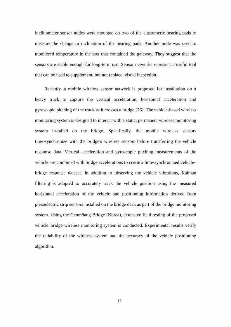
Recently, a mobile wireless sensor network is proposed for installation on a

heavy truck to capture the vertical acceleration, horizontal acceleration and

gyroscopic pitching of the truck as it crosses a bridge [76]. The vehicle-based wireless

monitoring system is designed to interact with a static, permanent wireless monitoring

system installed on the bridge. Specifically, the mobile wireless sensors

time-synchronize with the bridge's wireless sensors before transferring the vehicle

response data. Vertical acceleration and gyroscopic pitching measurements of the

vehicle are combined with bridge accelerations to create a time-synchronized vehicle–

bridge response dataset. In addition to observing the vehicle vibrations, Kalman

filtering is adopted to accurately track the vehicle position using the measured

horizontal acceleration of the vehicle and positioning information derived from

piezoelectric strip sensors installed on the bridge deck as part of the bridge monitoring

system. Using the Geumdang Bridge (Korea), extensive field testing of the proposed

vehicle–bridge wireless monitoring system is conducted. Experimental results verify

the reliability of the wireless system and the accuracy of the vehicle positioning

algorithm.

18

CHAPHER 3 WIRELESS SENSOR NETWORKS

3.1 Introduction to Wireless Sensor Networks (WSN)

Recently, advanced micro-electro-mechanical systems (MEMS) technology,

wireless communications, and electronics engineering have improved the

development of WSN. WSN is based on wireless sensor nodes. These tiny wireless

sensor nodes, which consist of sensing, processing, and communicating components,

collaborate with each other via wireless communication.

WSN have great potential for many applications in different scenarios such as

natural disaster monitoring [77], military target tracking and surveillance [78],

biomedical health care [14], and hazardous environment investigation and seismic

sensing [79]. In military target tracking and surveillance, a WSN can assist army to

detect and identify enemy target such tank movements as spatially-correlated and

coordinated troop. With natural disasters, wireless sensor nodes were used to sense

and detect the environment to forecast disasters before they occur. In biomedical care

applications, the wireless sensors can help monitor a patient’s health in surgical. For

seismic sensing, deployment of large numbers of wireless sensors along the volcanic

area can detect the development of earthquakes and eruptions.

A wireless ad hoc network is a kind of wireless technology. It is decentralized

type of wireless network. The network does not rely on a preexisting infrastructure.

Instead, each node forward data dynamically based on the network connectivity. Ad

hoc networks can use flooding for forwarding the data. There are differences between

WSN ad hoc networks. The differences between WSN and ad hoc networks was

19

illustrate below [80]:

i. The number of sensors in a WSN can be several orders of magnitude higher than

an ad hoc network.

ii. Sensor nodes are densely deployed in field.

iii. Sensor nodes are expected to failures in WSN.

iv. The topology of a sensor network changes when sensor node failure.

v. WSN mainly use broadcast or tree communication paradigm whereas most ad

hoc networks are based on point-to-point communications.

vi. WSN are limited in power, computational capacities, and memory.

Yick [81] classified the WSN into five types: terrestrial WSN, underground WSN,

underwater WSN, multi-media WSN, and mobile WSN. Terrestrial WSNs typically

consist of hundreds to thousands of inexpensive wireless sensor nodes deployed in a

application area. For deploying WSN, sensors can generally either deterministically or

randomly be placed in an area of interest [82]. The type of sensors determines the

choice of the deployment scheme rely on application and the environment. A viable

controlled node deployment is necessary when sensors are expensive or when their

operation is significantly affected by their position. Such scenarios include

underwater WSN applications, highly precise seismic monitoring, and placing

imaging and video sensors. Moreover, in some applications random distribution of

wireless sensor nodes is the necessary option. This is chiefly fact for harsh

environments such as a battle field or a disaster region. Depending on the node

distribution and the level of redundancy, random node deployment is considered a

good approach that can achieve the required performance goals.

20

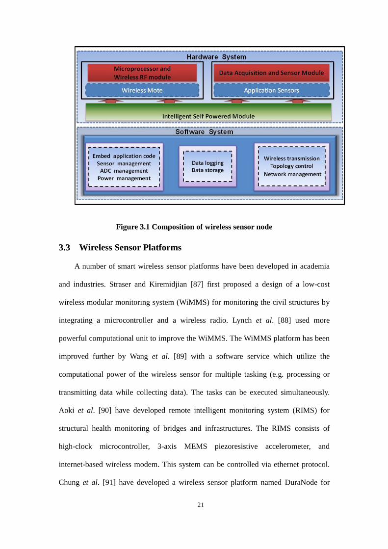
3.2 Subsystem of Smart Wireless Sensor Node

In this section, the subsystems of a smart wireless sensor are discussed. Figure

3.1 shows the composition of wireless sensor node. Generally, a smart wireless sensor

is composed of three or four functional subsystems: on-board micro-processor unit,

sensing unit, wireless communication unit, and power unit [12, 83]. The

computational micro-processor was generally used for the computational tasks. For

SHM application, to convert analogue sensor outputs to a digital format, the ADC

with a resolution of 16 bits or higher is needed. The sensing unit always includes an

ADC to connect sensors. For capturing low-order global response modes of a civil

structure, the wireless sensing unit should be designed to record response data at

sample rates at least 100 Hz. To capture high-order response modes of structural

components of civil structure, the wireless sensing unit should therefore need

relatively as high as possible sample rates (greater than 500 Hz) [12, 84]. The random

access memory (RAM) was used to stack the measured and processed data. A flash

memory with software programs was used for the system operation and data

processing [85]. A 16 bit digital sensor data could be stored at one time, at least 256

KB of RAM is required for a WSN application. For the simultaneous multiple tasks

application, at least approximately 256 KB of flash memory would be provided for

that purpose [84]. The wireless communication unit is used to communicate with

other wireless sensor nodes and to transfer the sensing data using a RF radio modem

and antenna Lower data loss rate is necessary for the highly reliable wireless

communication in the conditions of channel interference, multi-path reflections and

path losses. Radio signals always decrease as they propagate through structural

materials such as reinforced concrete or steel material and the large scale civil

structures require wireless communication ranges of at least 100 m. [12, 84, 86].

21

Figure 3.1 Composition of wireless sensor node

3.3 Wireless Sensor Platforms

A number of smart wireless sensor platforms have been developed in academia

and industries. Straser and Kiremidjian [87] first proposed a design of a low-cost

wireless modular monitoring system (WiMMS) for monitoring the civil structures by

integrating a microcontroller and a wireless radio. Lynch et al. [88] used more

powerful computational unit to improve the WiMMS. The WiMMS platform has been

improved further by Wang et al. [89] with a software service which utilize the

computational power of the wireless sensor for multiple tasking (e.g. processing or

transmitting data while collecting data). The tasks can be executed simultaneously.

Aoki et al. [90] have developed remote intelligent monitoring system (RIMS) for

structural health monitoring of bridges and infrastructures. The RIMS consists of

high-clock microcontroller, 3-axis MEMS piezoresistive accelerometer, and

internet-based wireless modem. This system can be controlled via ethernet protocol.

Chung et al. [91] have developed a wireless sensor platform named DuraNode for

22

monitoring bridges and buildings. DuraNode not only has a special feature for

wireless sensing but also allows the wired internet data communication for building

structures using an established Local Area Network (LAN). Farrar and Allen [92]

have developed a smart wireless sensor platform, called Husky. This platform

performs a series of damage detection algorithms by embedding a Java-based damage

detection algorithm package (DIAMOND II). Chen and Liu [93] presented a mobile

agent approach for enhancing the flexibility and reducing raw data transmission in

wireless structural health monitoring sensor networks. In their approach, they

developed an integrated wireless sensor network consisting of a mobile agent-based

network middleware and distributed high computational power sensor nodes. A

mobile agent system called Mobile-C was embedded this mobile agent middleware.

The mobile agent middleware allows a sensor network moving dynamically to the

data source. With mobile agent middleware, a sensor network is able to be

implemented in newly developed diagnosis algorithms and can be adjusted in

response to operational or task changes.

Besides the smart wireless sensor platforms developed in the academia, a number

of commercial smart wireless sensor platforms have been also developed for SHM

applications in the industries. Mica Motes, which is initially developed at the

University of California-Berkeley and subsequently commercialized by Crossbow Inc.,

may be the most famous commercialized wireless sensor platform. The Mote is an

open source wireless sensor platform with both its hardware and software. Motes is

very popular to the public [12]. The Wisden was design for structural data acquisition.

The Wisden perform wavelet-based compression techniques to overcome the

bandwidth limitations based on Mica2 motes platform [94]. Mica mote and

piezoelectric sensors then integrated for a parallel distributed structural health

23

monitoring system. The developed system can successfully monitor the concentrated

load position or a loose bolt position [95]. The performance of the mica mote was

investigated through a two story steel structure testing on shaking table. The results

shows that Mica mote can get the sufficient performance for the intended purpose

[96]. Mote has been successively revised to Imote and Imote2 by Intel. The Imote2

may be the most powerful and promising smart wireless sensor platform for SHM. It

built with 32 bit XScale processor with a RAM of 32 MB and a flash memory of 32

MB, and an integrated radio with a built-in 2.4 GHz antenna. Nagayama et al. [11]

successfully implemented a decentralized computing strategy in a wireless smart

sensor networks that used Imote2 for system identification. In their study, the

measured data was aggregated locally by a selected sensor node within the

communication distance in sensor group, and only limited pre-processed data was sent

back to the base station to locate the health of the structure.

3.4 Factors Influencing Sensor Network Design

Based on lacking of power, having physical damage or environmental

interference, some sensor nodes may fail or be blocked. The failure of sensor nodes

should not affect the overall task in WSN. Therefore, the reliability or fault tolerance

issue should be considered. Robust fault tolerance is the ability to endure sensor

network functionalities without any interruption due to sensor node failures [97].

In studying a different phenomenon, the hundreds or thousands number of sensor

nodes may be deployed. Depending on the application, the number may reach an

extreme value of millions. The new WSN approaches must be able to deal with this

number of nodes. The high density nature of the sensor networks can be less than 10

m in diameter for some specific applications [98].

24

The cost of a single node is very important to influence the overall cost in WSN

with a large number of sensor nodes. If the cost of the WSN is more expensive than

deploying traditional sensors, then the WSN is out of its benefit. It is why the cost of

each sensor node has to be kept low. For example, the novel technology allows a

Bluetooth radio system to be less than 10$ [99]. Also, the cost of a sensor node should

be much less than 1$ in order for the WSN to be feasible in the future.

The size of sensor node may be another important issue in some WSN

applications. The required size may be smaller than even a cubic centimeter which is

light enough to remain suspended in the air [100]. Apart from the size, there are also

some other constraints for designing a sensor node. These nodes must [101]

i. Consuming in extremely low power,

ii. Operating in high volumetric densities,

iii. Having low production cost and be dispensable,

iv. Operating unattended,

v. Be adaptive to the environment.

Sensor nodes are densely deployed to record different phenomenon. Therefore,

they usually work isolated in remote geographic areas. They may be working

i. in busy intersections,

ii. in the interior of a large machinery,

iii. at the bottom of an ocean,

iv. inside a twister,

25

v. on the surface of an ocean during a tornado,

vi. in a biologically or chemically contaminated field,

vii. in a battlefield beyond the enemy lines,

viii. in a home or a large building,

ix. in a large warehouse,

x. attached to animals,

xi. attached to fast moving vehicles, and

xii. in a drain or river moving with current.

3.5 The 802.15.4 and Zigbee Standards

The ZigBee Alliance [102] is an association of companies working together to

develop reliable, cost-effective, low-power wireless networking standard. ZigBee

technology was applied in a wide range of products and applications across consumer,

commercial, industrial and government markets worldwide. ZigBee builds upon the

IEEE 802.15.4 standard which defines the physical and MAC layers for low cost, low

rate wireless application. ZigBee defines the network layer specifications for star, tree

and peer-to-peer network topologies and provides a framework for application

programming in the application layer. Figure3.2 shows the 802.15.4 and Zigbee

Architecture. The following subsections give more details on the IEEE and ZigBee

standards.

26

Figure 3.2 802.15.4 and Zigbee Architecture

IEEE 802.15.4 standard

The IEEE 802.15.4 standard [103] defines the protocol of the physical and MAC

layers for Low-Rate Wireless Personal Area Networks (LR-WPAN). The advantages

of an this standard maintaining a simple and flexible protocol stack that are ease of

installation, reliable data transfer, short-range operation, extremely low cost, and a

reasonable battery life.

The physical layer supports three frequency bands and 27 channels with Direct

Sequence Spread Spectrum (DSSS) access mode: a 2450 MHz band (with 16

channels), a 915 MHz band (with 10 channels) and a 868 MHz band (1 channel), all

using the. The 2450 MHz band employs Offset Quadrature Phase Shift Keying

(O-QPSK) for modulation. The 868/915 MHz bands rely on Binary Phase Shift

Keying (BPSK). In addition to radio on/off operation, the physical layer supports

functionalities for channel selection, link quality estimation, energy detection

IEEE 802.15.4 MAC

Applications

IEEE 802.15.4

2400 MHz

PHY

IEEE 802.15.4

868/915 MHz

PHY

• Network Routing

• Address

translation

• Packet

Segmentation

• Profiles

ZigBee

•Packet generation

•Packet reception

•Data transparency

•Power Management

•Channel acquisition

•address

•Error Correction

27

measurement and clear channel assessment.

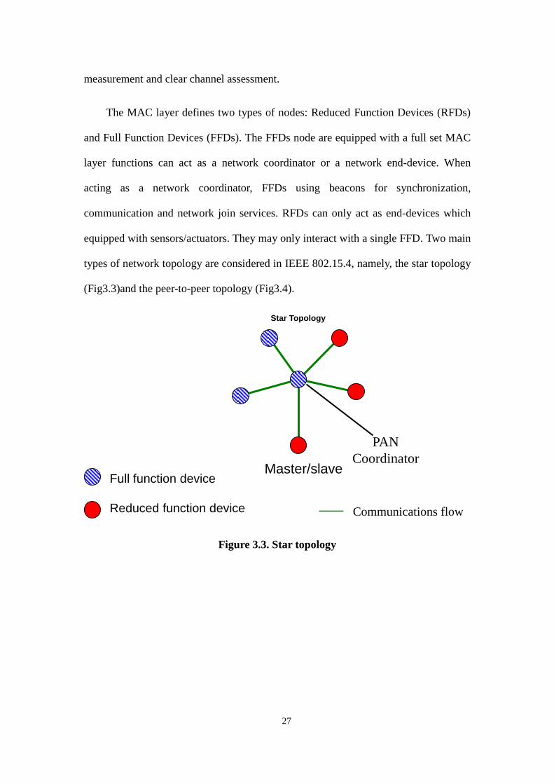
The MAC layer defines two types of nodes: Reduced Function Devices (RFDs)

and Full Function Devices (FFDs). The FFDs node are equipped with a full set MAC

layer functions can act as a network coordinator or a network end-device. When

acting as a network coordinator, FFDs using beacons for synchronization,

communication and network join services. RFDs can only act as end-devices which

equipped with sensors/actuators. They may only interact with a single FFD. Two main

types of network topology are considered in IEEE 802.15.4, namely, the star topology

(Fig3.3)and the peer-to-peer topology (Fig3.4).

Figure 3.3. Star topology

Full function device

Reduced function device Communications flow

Master/slave

PAN

Coordinator

Star Topology

28

Figure 3.4. Peer-to-peer topology

The ZigBee standard

ZigBee [102] deals with the higher layers of the protocol stack. The network

layer (NWK) organizes and provides routing over a multihop network (built on top of

the IEEE 802.15.4 functionalities). The Application Layer (APL) provide a interface

for distributed application development and communication. The APL comprises the

Application Framework, the ZigBee Device Objects (ZDO), and the Application Sub

Layer (APS). In the Application Framework, user can defined have up to 240

Application Objects of a ZigBee application. The ZDO provides services that allow

the application objects to discover each other and to organize into a distributed

application. The APS offers an interface to data and security services to all application

objects and ZDO.

ZigBee identifies three device types. A ZigBee end-device is corresponding to an

IEEE RFD or FFD for a simple task. A ZigBee router is an FFD with routing

capabilities. The ZigBee coordinator is an FFD for managing the whole WSN. The

Full function device Communications flow

Point to point Cluster tree

Peer-Peer Topology

29

ZigBee network layer supports more complex topologies like the tree and the mesh

while the IEEE 802.15.4 naturally uses the star topology. Multihop routing, route

discovery and maintenance, security and joining/leaving a network are among the

functionalities provided by the network layer with consequent short (16-bit) address

for assigning to newly joined devices.

3.6 Operating Systems for Wireless Sensor Networks

As the technology moving on, from its root in the Computer Science and

Electronic Engineer community, TinyOS has been adopted as an easy used WSN

operation system in more and more application fields, like Civil Engineering.

TinyOS is designed for low power, ad-hoc, and embedded sensor networks; it is

a component based and event driven operation system which make it a very flexible

and easy to use. These features make TinyOS easy to deploy in different WSN

platforms like Mica, TelosB, Imote2, EYES, BTNode, also Gains and Hawk platform

from China. Although the low level hardware devices are different, researchers who

work on it could use similar environment and share their work results by the

component mechanism.

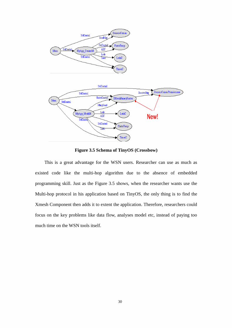
30

Figure 3.5 Schema of TinyOS (Crossbow)

This is a great advantage for the WSN users. Researcher can use as much as

existed code like the multi-hop algorithm due to the absence of embedded

programming skill. Just as the Figure 3.5 shows, when the researcher wants use the

Multi-hop protocol in his application based on TinyOS, the only thing is to find the

Xmesh Component then adds it to extent the application. Therefore, researchers could

focus on the key problems like data flow, analyses model etc, instead of paying too

much time on the WSN tools itself.

New!

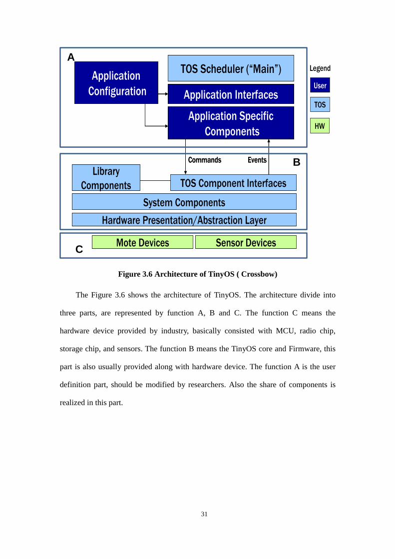
31

Figure 3.6 Architecture of TinyOS ( Crossbow)

The Figure 3.6 shows the architecture of TinyOS. The architecture divide into

three parts, are represented by function A, B and C. The function C means the

hardware device provided by industry, basically consisted with MCU, radio chip,

storage chip, and sensors. The function B means the TinyOS core and Firmware, this

part is also usually provided along with hardware device. The function A is the user

definition part, should be modified by researchers. Also the share of components is

realized in this part.

Hardware Presentation/Abstraction Layer

Mote Devices Sensor Devices

TOS Scheduler (“Main”)

System Components

Library

Components TOS Component Interfaces

Application

Configuration

Application Specific

Components

Application Interfaces

EventsCommands

Hardware Presentation/Abstraction Layer

Mote Devices Sensor Devices

TOS Scheduler (“Main”)

System Components

Library

Components TOS Component Interfaces

Application

Configuration

Application Specific

Components

Application Interfaces

EventsCommands

TOS

User

Legend

HW

A

C

B

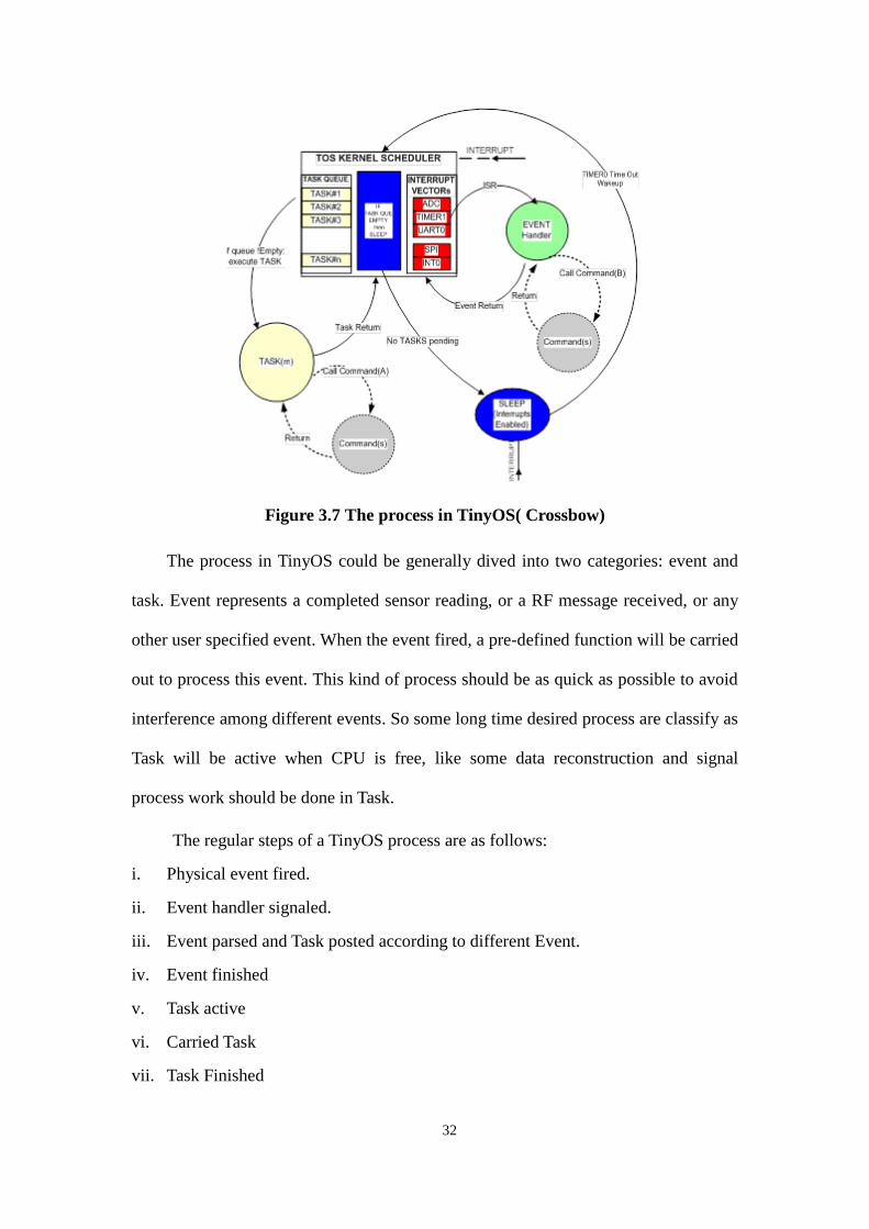
32

Figure 3.7 The process in TinyOS( Crossbow)

The process in TinyOS could be generally dived into two categories: event and

task. Event represents a completed sensor reading, or a RF message received, or any

other user specified event. When the event fired, a pre-defined function will be carried

out to process this event. This kind of process should be as quick as possible to avoid

interference among different events. So some long time desired process are classify as

Task will be active when CPU is free, like some data reconstruction and signal

process work should be done in Task.

The regular steps of a TinyOS process are as follows:

i. Physical event fired.

ii. Event handler signaled.

iii. Event parsed and Task posted according to different Event.

iv. Event finished

v. Task active

vi. Carried Task

vii. Task Finished

33

There are two types of component; module and component. Components is

written with code and wired together as a Configuration to create a Mote application.

The interface provides two methods, ―provide‖ and ―use‖, to wire the components.

The table 3.1 shows all description of keywords in TinyOS.

Table 3.1 Description of keywords in TinyOS.

Keword Description

interface A collection of event and command definitions

module A basic component implemented in nesC.

configuration A component made from wiring other components.

implementation Contains code & variables for module or

configuration.

components List of components wired into a configuration.

provides Defines interfaces provided by a component.

uses Defines interfaces used by a module or configuration.

as Alias an interface to another name.

command Direct function call exposed by an interface.

event Callback message exposed by an interface.

Due to the limited memory, the memory usage and memory space need to be

managed. The TinyOS uses the static memory model to manage the memory. The

components of static memory model are statically linked together and size required

determined at compile time. The global variables are used to conserve memory and

the pointers are also using here.

34

TinyOS, the innovation operation system enables researchers to implement their

own WSN research easily, enables researchers share their code and research result all

over the world instead of building everything by oneself, enables an entry level

researcher build up a prototype system very easily and quickly. Plenty of component

based libraries, supporting mesh protocols, distributed services, data acquisition tools

and QoS service, which makes user easy to construct the individual application with

high efficiency and reliability. However, for civil engineers, students and researchers,

using TinyOS to develop the individual SHM application are not very easily. A new

WSN development environment should be developed.

3.7 Time Synchronization

In wireless sensor networks, the data fusion is a basic operation. Data from each

sensor is collected by a data fusion center [104]. The fusion of individual sensor uses

exchanging messages that are time stamped by each sensors local clock. This task

needs an exact time among the sensors. Protocols that provide exact time clock are

synchronization protocols. Over the past few decades, researchers have developed

successful clock synchronization protocols for wired networks. However, these

protocols are unsuitable for a WSN because the challenges posed by WSN are

different and manifold from wired networks.

There is several facts influence synchronization in WSN. The major error in time

synchronization schemes is the message delivery delay with non-determinism in the

latency estimating. A description of sources of synchronization error was first

described by Koeptz [105] and extended recently by Horauer et. al. [106].

The main time synchronization errors are shown below [106]:

(1). Send Time: The delay in the packet traversal from the message assembly

35

at the application layer all the way down to MAC layer. Highly

non-deterministic.

(2). Access Time: Is the channel contention time, that in dense broadcast

medium such as ours can be in the order of hundreds of milliseconds.

Least deterministic part of the message delivery.

(3). Interrupt Handling Time: The delay between the radio chip raising and

the microcontroller responding to an interrupt. Can be an issue if

interrupts are disabled on the microcontroller.

(4). Transmission and Reception Time:The delay in sending or receiving the

entire length of the packet over the channel. Largely deterministic, is a

function of bandwidth and packet size.

(5). Propagation Time: The delay, for a particular symbol of the message, in

traversing all the way to the receiver. The propagation time can be

deterministic if the speed of propagation is assumed constant, and

endpoint location is known, or if synchronization exchange is performed

with assumption of path symmetry. This delay can be significant in the

underwater acoustic channel since assuming clocks will not skew over

packet exchanges would be incorrect.

Basically, there are two schemes to synchronize clocks: Sender-Receiver and

Receiver- Receiver. All synchronization schemes developed within these two basic

frameworks. Network Time Protocol (NTP) is widely used in the Internet. It is

approach works well with high latency and high variability [107]. The NTP protocol

estimates both offset and skew using long-term, bi-directional exchange of time

information. Unfortunately, NTP is a poor match for WSN for several reasons. First, it

36

assumes communications are relatively inexpensive. However theWSN are bandwidth

and energy constrained. Next, NTP is designed for constant low rates operation in the

background. (At a maximum polling rate of 16 sec, NTP took around an hour to

reduce error to about 70us). On the other hand, TSHL (Time Synchronization for High

Latency)[108] exchanges number of broadcast beacons to compute skew and then

perform one bidirectional exchange to compute a skew-corrected offset. Generally,

TSHL and NTP synchronize clock using the same time information, however TSHL

reduces energy consumption using a smaller number of broadcast beacons by

replacing long-term bidirectional communication.

37

CHAPHER 4 INTEGRATED WSN-based SHM

SYSTEM

4.1 Introduction

Characterized by its low manufacturing cost, low power requirement,

miniaturized size, and no need for cabling, the wireless sensor networks (WSN) has

emerged as an attractive sensing technology for deploying dense distributed

sensors[12, 13]. Among the various wireless monitoring techniques [12-17], the

MICA mote is a commercially available product that has been used extensively by

researchers and developers. It utilizes an Atmel ATmega 128L processor that runs at 4

MHz. The 128L is an 8-bit microcontroller that has 128 kilobytes of onboard flash

memory to store the mote's program. MICA motes have certain limitations, including

limited sampling rate, processing ability, storage, and transmission ability. In

comparison, the advanced wireless sensor platform Imote2 is considered as a better

choice for developing and deploying customized wireless sensor networks efficiently

[109, 110]. While the WSN-based sensing system is accessible and achievable,

development beyond a prototype towards full-scale structure applications often incurs

hardware and software complexities, making it quite challenging, especially for civil

engineers with limited WSN experience. Also, robust system development is

problematic under a complex programming environment. To this end, this thesis

presents an easy-to-use development environment based on the .NET Micro

Framework (NETMF). Applications can be implemented efficiently under the

NETMF. Evidently, the accelerated development of the SHM techniques can be partly

attributed to the user-friendly environment brought by the WSN.

38

This chapter discusses the architecture for proposed Integrated WSN-based SHM

system. This system is developed based on NETMF platform, which is an advanced

sensor platform compatible with NETMF. Architecture, wireless sensor node design,

energy harvesting system, software framework, and WSN-Based SHM service to be

employed in this thesis are described.

4.2 Architecture of Integrated WSN SHM System

The proposed integrated WSN-based SHM system is shown in Fig.4.1. This

system is based on hybrid wireless communication, structural conditions will be

assessed remotely. The proposed architecture consists of sensing nodes, cluster head

nodes, transfer node, and base station. The purpose of sensing node is to measure the

responses of structure or the environmental parameters. They are deployed in

structure to perform specific tasks such as sensing, data processing, and

acknowledgement. Each sensing node is based on Imote2 platform which is

comprised of a microprocessor, sensor module, and communication device. All

sensing data will be sent to a cluster head nodes in their own community using one

hop transmission.

Cluster head node can communicate with the sensing nodes or other cluster

heads of the neighboring communities to exchange information or triggering sensing

task. The cluster head is a dule core design which combine Imote2 platform and

second embedded device. The cluster head has extra wireless module and GPS. The

extra wireless module has more powerful RF power can increase the wireless

communication distance. The GPS is useful for synchronization and localization

purposes. The transfer node is functions as coordinate node for managing the cluster

heads and hoping the data. The sensing data will be sent to the base station, if needed,

39

using fast communication device such as WiFi. The base station is the highest level

end device that has largest memory, most powerful processor and highest

communication capability. The base station node is the gateway between smart sensor

networks and the Host computer. The base station uploads the data to remote

monitoring and control server via satellite, 3G telecommunication or WiMAX

communication. A Host computer may be needed in this architecture as an interface to

sends commands and parameters to smart sensor networks via the base station.

Figure 4.1 Integrated WSN-based SHM system architecture: different roles are

assigned to nodes

4.3 Hardware Design

This section shows all hardware design of wireless sensor nodes which are

proposed and employed in this study. The proposed wireless sensor nodes are sorted

into sensing nodes, cluster head nodes, transfer node, and base station.

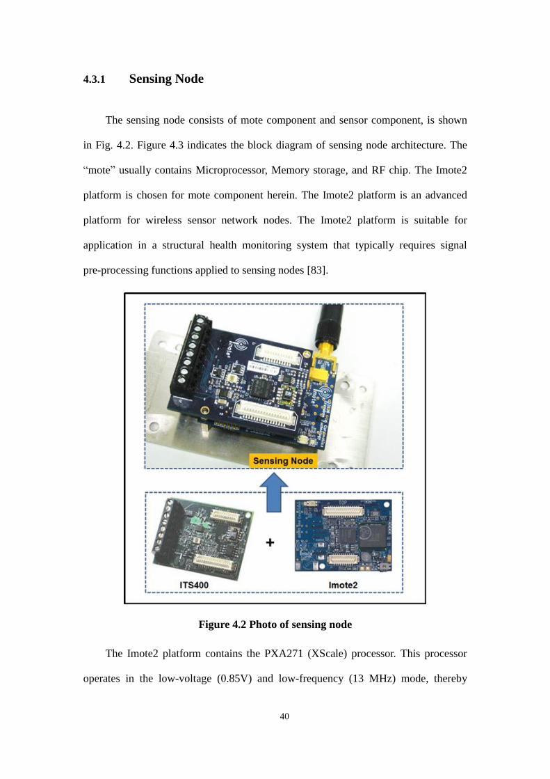
40

4.3.1 Sensing Node

The sensing node consists of mote component and sensor component, is shown

in Fig. 4.2. Figure 4.3 indicates the block diagram of sensing node architecture. The

―mote‖ usually contains Microprocessor, Memory storage, and RF chip. The Imote2

platform is chosen for mote component herein. The Imote2 platform is an advanced

platform for wireless sensor network nodes. The Imote2 platform is suitable for

application in a structural health monitoring system that typically requires signal

pre-processing functions applied to sensing nodes [83].

Figure 4.2 Photo of sensing node

The Imote2 platform contains the PXA271 (XScale) processor. This processor

operates in the low-voltage (0.85V) and low-frequency (13 MHz) mode, thereby

41

enabling low-power operation. The processor can be scaled to 104 MHz at the lowest

voltage and increased to 416MHz using dynamic voltage scaling. The Imote2

platform can perform complex signal processing functions, such as FFT and image

compressing. The Imote2 platform contains 256 KB of SRAM divided into four equal

64KB banks. The PXA271 of the Imote2 platform is a multi-chip module that has

three chips in a single package—the processor, 32 MB of SDRAM, and 32 MB of

flash memory. Such a memory improvement is a significant advantage compared with

the 4kB of RAM in Mica motes. The sensing task must store a massive amount of

sample data in external flash memory. The write/read data rate is limited by one slow

hardware device. However, the Imote2 platform stores sample data in RAM instead of

the complex and slow flash write function. The processor integrates many I/O options,

making it extremely flexible in supporting different sensors, A/Ds, and radio options.

These I/O options are I2C, three synchronous serial ports, three high-speed UARTs,

GPIOs, SDIO, USB client and host, AC97 and I2S audio codec interfaces, a fast

infrared port, PWM, a camera interface, and high-speed bus. The Imote2 platform

uses the CC2420 IEEE 802.15.4 radio transceiver, which supports a 250 Kbps data

rate with 16 channels in the 2.4GHz band.

42

Figure 4.3 Block diagram of sensing node architecture.

Table 4.1 compares mote platforms which are widely used in many research

groups. It can be seen in the table that the transmission range of RIRS is 300 m

outdoor, two to three times than other motes. The power consumption of TelosB is

much lower than other motes. For SHM application, high sampling rate sensing

always get great amount of data. By comparison, although Imote2 does not

outperform other motes in power consumption and transmission range, the larger

memory is more suitable for SHM application. The larger memory is beneficial for

smart sensor applications, which is require multiple tasks, such as wireless

communication, data logging, data acquisition, and in-situ signal processing.

The sensor component is ITS400 herein. The ITS400 sensor board is designed to

connect to the basic connectors on the Imote2. It contains a ST Micro LIS3L02DQ 3d

accelerometer, SHT15 temperature/humidity sensor, TAOS TSL2651Light Sensor and

43

Maxim MAX1363 4 Channel General Purpose A/D. This Accelerometer board has a

range of +/- 2g with 12 bit resolution. It communicates to Imote2 with two possible

interfaces, SPI or I2C. By default, the sensor is connected to SSP1 on the Imote2.

On board SHT15 sensor can be used for requiring high accuracy temp reading

(+/- 0.3 degC) and humidity. This sensor interfaces to the Imote2 through two GPIO

pins. The data pin of the SHT11 is connected to GPIO 100, whereas the clock pin is

connected to GPIO 98. The TAOS TSL2651 light sensor interfaces to the Imote2

through the I2C bus. The interrupt pin is connected to GPIO99 through a NAND gate.

If GPIO 99 conflicts with another board, the BT_TXD pin can be used instead by

loading R35. The board includes a Maxim MAX1363, 4 channel, 12 bit resolution

general purpose ADC for quick prototyping. Each channel supports 0-3 V input

signals. The ADC interfaces to the Intel Mote 2 through the I2C bus. The analog pins

are brought out to a Molex PN-39357-0003 connector (J5).

Table 4.1 Comparison of mote platform

MICA2 MICAZ IRIS TelosB Imote2

Processor ATmega128L ATmega128L ATmega128L MSP430 XScalePXA271

Clock

speed(MHz) 7.37 7.34 16 6.7 13-416

Bus size(bits) 8 8 8 16 32

Program Flash

Memory(bytes) 128 k 128 k 128 k 48 k 32 M

EEPROM (bytes) 4 k 4 k 4 k 16 k

RAM (bytes) 4 k 4 k 4 k 10 k 256 k+ 32 M

external

ADC 10 bit 10 bit 10 bit 12 bit N/A

Active power(mA) 8 8 8 1.8 31@13 MHz

44

Sleep power(uA) 15 15 8 5.1 390

Measurement

Flash(bytes) 512 k 512 k 512 k 1024 k 32 M

RF Chip CC1000 CC2420 At86rf230 CC2420 CC2420

Frequency(MHz) 2400-2483.5 2400-2483.5 2400-2483.5 2400-2483.5 2400-2483.5

Data rate (kbps) 38.4 250 250 250 250

Transmission

power (dbm) -20-5 -24-0 3 -24-0 -24-0

Outdoor range 150 m 100 300 100 100

Indoor range 30 m 30 50 30 30

Typica supply

voltage 3.3 V 3.3 V 3.3 V 3.3 V 4.5 V

Size (mm) 58 x 32 x 7 58 x 32 x 7 58 x 32 x

7

65 x 31 x

6 36x 48 x 9

Weight (g) 18 18 18 23 12

4.3.2 Cluster Head and Transfer Node

The cluster head node is a dule core design which combines Imote2 platform and

second embedded device FEZ domino platform, which contains extra wireless module

and GPS. Figure 4.4 and 4.5 show the Block diagram of Cluster Head node

architecture and photograph of Cluster Head node on a box. Cluster head nodes are in

charge of collecting data from sensing nodes and managing data; these nodes have

45

features such data storage on SD card or USB memory devices, database support,

Runtime Loadable Procedure (RLP), which is used to implement intensive data

processing function and time-critical routines such as FFT. The Transfer node has the

same hardware design to cluster head node without Imote2.

Domino is a tiny open-source board based on ARM7 microcontroller from NXP

running Microsoft NETMF. With this sophisticated combination, a developer can

easily control this microcontroller IOs and interfaces such as SPI, UART (Serial Port)

and I2C with simple unified managed code (C# code). Many libraries have already

included similar FAT file system, threading, USB Client, USB Host, UART, SPI, I2C,

GPIO, PWM, ADC, DAC, and many more.

The extra wireless module used herein is Digi XBee modules. XBee is a wireless

communication module that Digi built to the 802.15.4/ZigBee standard. These

modules communicate with the microcontroller using the UART. Table 4.2 gives the

specification of Xbee models. It can be seen in the table that the transmission range

can be designated by choosing specific model. It is useful for deploying WSN in large

scaled structure.

46

Figure 4.4 Block diagram of Cluster Head node architecture.

Table 4.2 Specification of Xbee models.

Model XB XB-Pro XB-ZB XB-ZB-Pro XB-868 XB-900 XB-XSC

Protocol 802.15.

4 802.15.4 Zigbee-Pro Zigbee-Pro RF RF RF

Frequenc

y 2.4GHz 2.4GHz 2.4GHz 2.4GHz

868MH

z

900MH

z 900MHz

Tx power 1mW 100mW 2mW 50mW 315mW 50mW 100mW

Sensitivity -92dB -100dBm -96dBm -102dBm -112dB

m

-100dB

m -106dBm

Range 500m 7000m 500m 7000m 40Km 10Km 24Km

47

Figure 4.5 Photograph of Cluster Head node on box

4.3.3 Base Station

The base station is the highest level device that can store a mass of data and

upload to remote center. The base station is based on ChipworksX Module.

ChipworkX Module is a small (67.6mmx47mm) ARM9 processor based board with

SO-DIMM200 slot interface and a very high performance. ChipworkX Module

supports a complete set of features such as FAT, USB device and many more. In

addition, it supports many other exclusive features, for example, USB host, PPP,

GPRS, 3G...etc. The sensing data can store and access using SD/MMC cards and USB

memory devices such as Thumb Drives and Hard Disks. Moreover, the USB host

function can access other devices like mice, keyboards, joysticks, printers, USB

modem and more. Furthermore, using SQLite database, allowing fast logging and

retrieving of standard SQL quires. For real-time and high processing needs, Runtime

48

Loadable Procedures, allow users to load their own compiled native code (C or

assembly).

Figure 4.6 Block diagram of base station architecture.

4.3.4 Multi-Sensor Board Design

This study developed a new sensor board which integrates a six degrees of

freedom inertial measurement unit (6 DoF IMU) SD746 sensor chip (SensorDynamics

Inc.) and a GPS module. The SD746 is used to measure acceleration and the GPS is

used to synchronize the sensing nodes. Figure 4.7 shows the simplified block

diagram of proposed 6 DoF-GPS sensor board. The chosen 6 DoF IMU is a

temperature-compensated and calibrated sensor that integrates functionality of 3-axis

gyro sensor and 3-axis accelerometer in one small package. Exposing the module to

accelerations and angular rates leads to small variations of the MEMS sensors

49

capacitances. Amplifier and ADC convert these changes in the gyro and accelerometer

capacitances into digital signals and then processed by dedicated Digital Signal

Processing (DSP) units. The DSP applies filtering, bias and sensitivity adjustment,

temperature compensation. Individual sensor configuration data are stored into a

non-volatile memory which contains also the individual serial number for production

and traceability. SPI and I2C communication interfaces share the same digital IOs. A

set of internal monitoring signals, continuously available though both SPI and I2C

interface allows the user to check the correct functionality of the entire module.

Figure 4.8 presents the photograph of the developed multi-sensor board. Table 4.3 and

4.4 shows the physical and electrical characteristics of gyro and accelerometer sensor.

Figure 4.7 Simplified Block Diagram of Multi-sensor board

u-bloxneo-5Q

GPS

3-Axis Gyro Sensor

3-Axis Accelerometer

ADC

UART

DSP SPI

UEXT connector

GPS bee

SD746

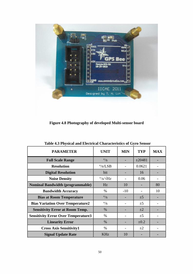
50

Figure 4.8 Photography of developed Multi-sensor board

Table 4.3 Physical and Electrical Characteristics of Gyro Sensor

PARAMETER UNIT MIN TYP MAX

Full Scale Range °/s - ±20481 -

Resolution °/s/LSB - 0.0621 -

Digital Resolution bit - 16 -

Noise Density °/s/√Hz - 0.06 -

Nominal Bandwidth (programmable) Hz 10 - 80

Bandwidth Accuracy % -10 - 10

Bias at Room Temperature °/s - ±5 -

Bias Variation Over Temperature2 °/s - ±5 -

Sensitivity Error at Room Temp. % - ±2 -

Sensitivity Error Over Temperature3 % - ±5 -

Linearity Error % - ±0.2 -

Cross Axis Sensitivity1 % - ±2 -

Signal Update Rate KHz 10 - -

51

Table 4.4 Physical and Electrical Characteristics of Accelerometer Sensor

PARAMETER UNIT MIN TYP MAX

Full Scale Range g - ±84 -

Resolution μg/LSB - 244.1 -

Digital Resolution bit - 16 -

Noise Density (mg)/√Hz - 0.28 -

Nominal Bandwidth (programmable) Hz 10 - 80

Bandwidth Accuracy % -10 - 10

Bias at Room Temperature g - ±0.05 -

Bias Variation Over Temperature2 g - ±0.2 -

Sensitivity Error at Room Temp. % - ±2 -

Sensitivity Error Over Temperature3 % - ±5 -

Linearity Error % - ±0.5 -

Cross Axis Sensitivity % - ±2 -

Signal Update Rate KHz 10 - -

The GPS module is designed based on NEO-5Q GPS chip (Ubox Inc.) and used

to synchronize the sensing nodes. The accuracy of timepulse signal is 40ns RMS. The

NEO-5Q has a 32-channel acquisition engine with over 1 million effective correlators

and is capable of massive parallel searches across the time/frequency space. This

enables a Time To First Fix (TTFF) of less than 1 second while long correlation/dwell

times make possible the best-in-class acquisition and tracking sensitivity. An available

functionality is KickStart, a new feature enabling accelerated acquisition of weak

signals. Once acquired, satellites are passed on to a power-optimized dedicated

tracking engine. This arrangement allows the GPS engine to simultaneously track up

to 16 satellites while searching for new ones. It has several features that are shown

below:

i. 50-channel u-blox 5 engine with over 1 million effective correlators

ii. <1 second Time To First Fix for Hot and Aided Starts

iii. -160dBm acquisition and tracking sensitivity

iv. Accelerated startup at weak signals for modules with KickStart feature

52

v. Supports AssistNow Online and AssistNow Offline A-GPS services; OMA

SUPL compliant

vi. 4 Hz position update rate

vii. Miniature 2.0mm pitch header, compatible with Xbee socket

4.3.5 Power Module

Power sources and power consumption are the critical issue in WSN if batteries

have to be periodically replaced. Hence, this study proposed a power module with

energy harvesting system and energy storage unit. The proposed theory is harvesting

the ambient energy like the vibration of the bridge to power the sensor device or to

recharge the primary battery. A novel energy harvesting based on piezoelectric

transducer was developed. Next section completed describes the proposed energy

harvesting system in detail.

4.4 Windmill-Magnet Integrated Piezoelectric (WMIP) Energy

Harvesting System

Although a wireless sensor network based structural health monitoring system

has many benefits, power sources and power consumption are the critical issue if

batteries have to be periodically replaced. Therefore, harvesting and storing the

ambient sources of energy to supply the sensor node seems to be an agreeable

approach. The sources of ambient energies typically include thermal, sunlight, wind,

RF and vibration energy. This study only considered the vibration based piezoelectric

energy harvesting approach. Several researches proposing and reviewing the possible

energy harvesting schemes can be found in the literature [111-114].

53

4.4.1 General Theory of Vibration-Based Energy Harvesting

Method

A single degree of freedom lumped spring mass system is mostly utilized to

model a vibration-based energy harvesting system. A diagram of a piezoelectric

cantilever beam with a proof mass at the end and a model of equivalent lumped spring

mass system is shown in Fig.4.8. The equation of motion of a single degree of

freedom (SDOF) system consisting of a mass m, a spring with spring constant k, and a

damping coefficient c under external excitation is described as

( ) ( ) ( ) ( )mz t cz t kz t my t (4.1)

where z is the net displacement. Assuming that the external excitation is harmonic

given as ( ) siny t Y t , the steady –state solution for the mass displacement is

given by

2

22 2

( ) sin

1 2

n

n n

z t Y t

(4.2)

where the is the phase angle given by

1

2tan

c

k m

(4.3)

The approximate mechanical power of a piezoelectric generator can be given by

54

3

2 3

22 2

1 2

n

n n

m Y

P

(4.4)

The maximum energy can be extracted by setting the excitation frequency to

match the natural frequency of the system and is given by

2 3

4

nmYP

(4.5)

Observing Eq. (4.5), it provides evidence that power can be optimized by

lowering damping, increasing natural frequency, mass, and amplitude of excitation.

Figure 4.9 (a) Cantilever beam with tip mass, (b) model of equivalent lumped

spring mass system

4.4.2 Energy Harvesting Circuits

A typical energy harvesting circuit, with piezoelectric generator, battery and

55

sensor, is shown in Fig.4.10. The piezoelectric material produces an ac voltage output

when the piezoelectric deformed. Therefore, this voltage needs to be converted to a dc

voltage before charging the capacitor. The four diodes form a bridge circuit to

perform a rectifier. Energy harvesters typically produce small amounts of energy over

long periods, therefore an energy storage component in the form of a supercapacitor

usually contain in harvesters system. A larger capacitor provides power for a longer

time for the same load but takes more time to charge it. Typical supercapacitor often

has a much lower voltage than standard electrolytic capacitors, a zener diode usually

used to prevent the voltage across the supercapacitor from increasing beyond its

maximum voltage rating. When applying a load, the supercapacitor discharging

immediately, and the voltage across the supercapacitor starts dropping. Hence, a

dc/dc-voltage-converter IC is used to assurance a fixed voltage at the output.

Figure 4.10 Typical piezoelectric harvesting circuit

The typical piezoelectric harvesting model can be improved via new energy

harvesting IC, LTC3588-1 (LINEAR TECHNOLOGY). This IC combines a low-loss

Piezoelectric generator

rectifier

dc/dc-voltage-

converterSupercapacitor

Sensor Battery

56

full-wave bridge rectifier with a high efficiency buck converter to form a tiny energy

harvesting component for an ambient energy harvesting. The peak load currents are

much higher than a piezoelectric generator can produce. Thus the LTC3588-1

accumulates energy that released to the load to supply the sensor or controller. For the

different purpose of applications, this IC provides four output voltages, 1.8V, 2.5V,

3.3V and 3.6V via two selectable pins. Typically, up to 100mA of continuous output

current can be provided; however, a higher output current can be supplied by way of

sizing the output capacitor. Base on this advanced energy harvesting IC, the

architecture of energy harvesting based wireless sensor node was shown in Fig.4.11. A

LTC3588-1 connects with piezoelectric generator and backup battery to supply the

sensor. This architecture proposed that when ambient energy is obtainable, the battery

is unloaded, but when the ambient source ceases, the battery initiates and serves as the

backup power supply. The backup battery must connect with a series blocking diode

connected to VIN pin to prevent reverse current flowing into the battery. Any stack of

batteries can be used as long as the battery voltage does not exceed 18V. One should

be considered that the peak voltage of piezoelectric generator should exceed the

battery voltage. This approach not only decreases the replacing time of battery, but it

also improves reliability and elasticity of sensing system. For instance, an energy

harvesting sensor node is deployed on a structure such as a bridge, may gather energy

when the vehicles pass through the bridge. However, in off-peak times the vehicles

are rarely and vibration is also low, a battery backup can still supplies the sensor node.

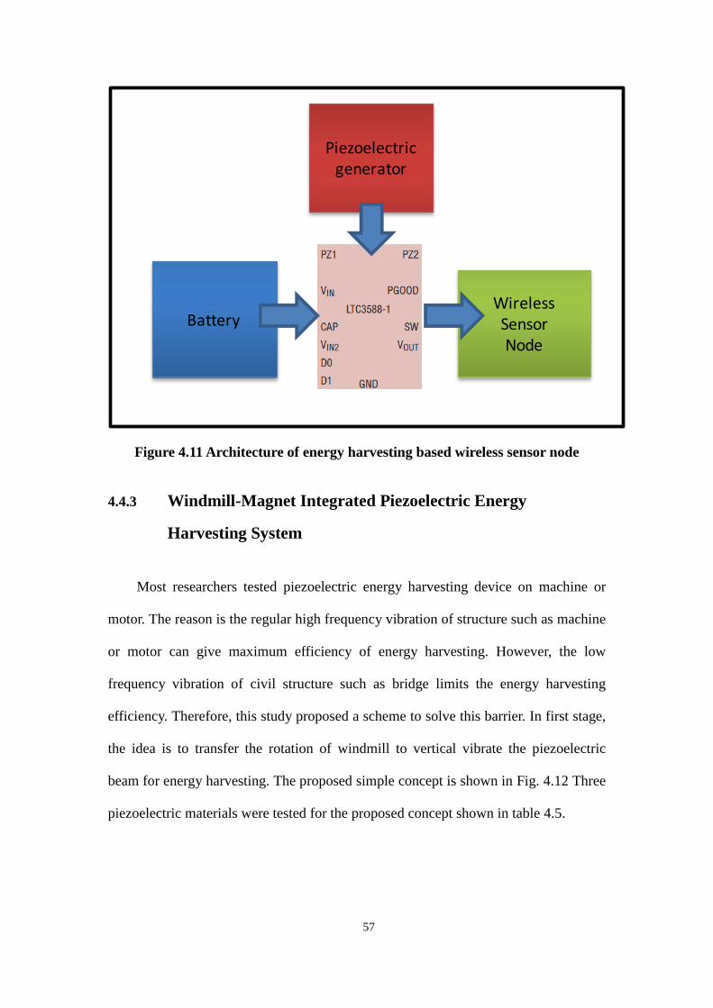
57

Figure 4.11 Architecture of energy harvesting based wireless sensor node

4.4.3 Windmill-Magnet Integrated Piezoelectric Energy

Harvesting System

Most researchers tested piezoelectric energy harvesting device on machine or

motor. The reason is the regular high frequency vibration of structure such as machine

or motor can give maximum efficiency of energy harvesting. However, the low

frequency vibration of civil structure such as bridge limits the energy harvesting

efficiency. Therefore, this study proposed a scheme to solve this barrier. In first stage,

the idea is to transfer the rotation of windmill to vertical vibrate the piezoelectric

beam for energy harvesting. The proposed simple concept is shown in Fig. 4.12 Three

piezoelectric materials were tested for the proposed concept shown in table 4.5.

Battery

Piezoelectric generator

Wireless SensorNode

58

Table 4.5 Different types of piezoelectric product

Type Dimension(length X

width)

Manufacturing

Company

PZT 60X20mm APC

MFC 85X28mm Smart Material

Raw Volture 100X25.4mm MIDE

Figure 4.12 Schematic diagram of windmill based piezoelectric harvesting system

Fig. 4.13 shows the experimental setup on overpass in Tokyo University. A

piezoelectric film was set as a cantilever beam mounted on a base which was fixed in

the bridge. Wind can drive the windmill to beat the piezoelectric film to output the

voltage. The Fig. 4.14 to 4.16 illustrates the output voltage of PZT, MFC and Raw

Volture respectively. As shown in Figure, the peak voltage represents the high voltage

output when the windmill beat the beam. The result also shows the MFC has high

voltage under the same excitation. The result confirms that the proposed windmill

based piezoelectric energy harvesting concept is practical. However, contact between

windmill and piezoelectric beam might stop the whirling of blade. To solve this

problem, a novel windmill-magnet integrated piezoelectric (WMIP) energy harvesting

system was proposed in Fig. 4.17. The proposed WMIP harvesting system integrates a

windmill, magnet and piezoelectric beam for energy harvesting. A magnet was

Transfer Mechanism

Piezoelectric beam

Transfer the rotation to vertical vibrate the Piezoelectric

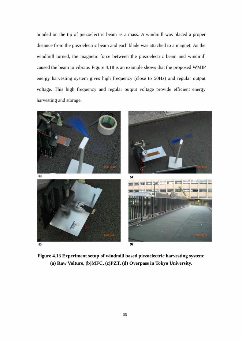
59

bonded on the tip of piezoelectric beam as a mass. A windmill was placed a proper

distance from the piezoelectric beam and each blade was attached to a magnet. As the

windmill turned, the magnetic force between the piezoelectric beam and windmill

caused the beam to vibrate. Figure 4.18 is an example shows that the proposed WMIP

energy harvesting system gives high frequency (close to 50Hz) and regular output

voltage. This high frequency and regular output voltage provide efficient energy

harvesting and storage.

Figure 4.13 Experiment setup of windmill based piezoelectric harvesting system:

(a) Raw Volture, (b)MFC, (c)PZT, (d) Overpass in Tokyo University.

60

Figure 4.14 Output voltage of PZT

Figure 4.15 Output voltage of MFC

61

Figure 4.16 Output voltage of Raw Volture

Figure 4.17 Windmill-magnet integrated piezoelectric (WMIP) energy harvesting

system

62

Figure 4.18 Output voltage and FFT of WMIP energy harvesting system

4.5 Three-Tier Software Framework

The proposed software system of integrated WSN-based SHM system is a

three-tier-framework, i.e., node, logging and processing tiers. Herein, the node tier

consists of developed application functions and is installed on all sensor nodes. The

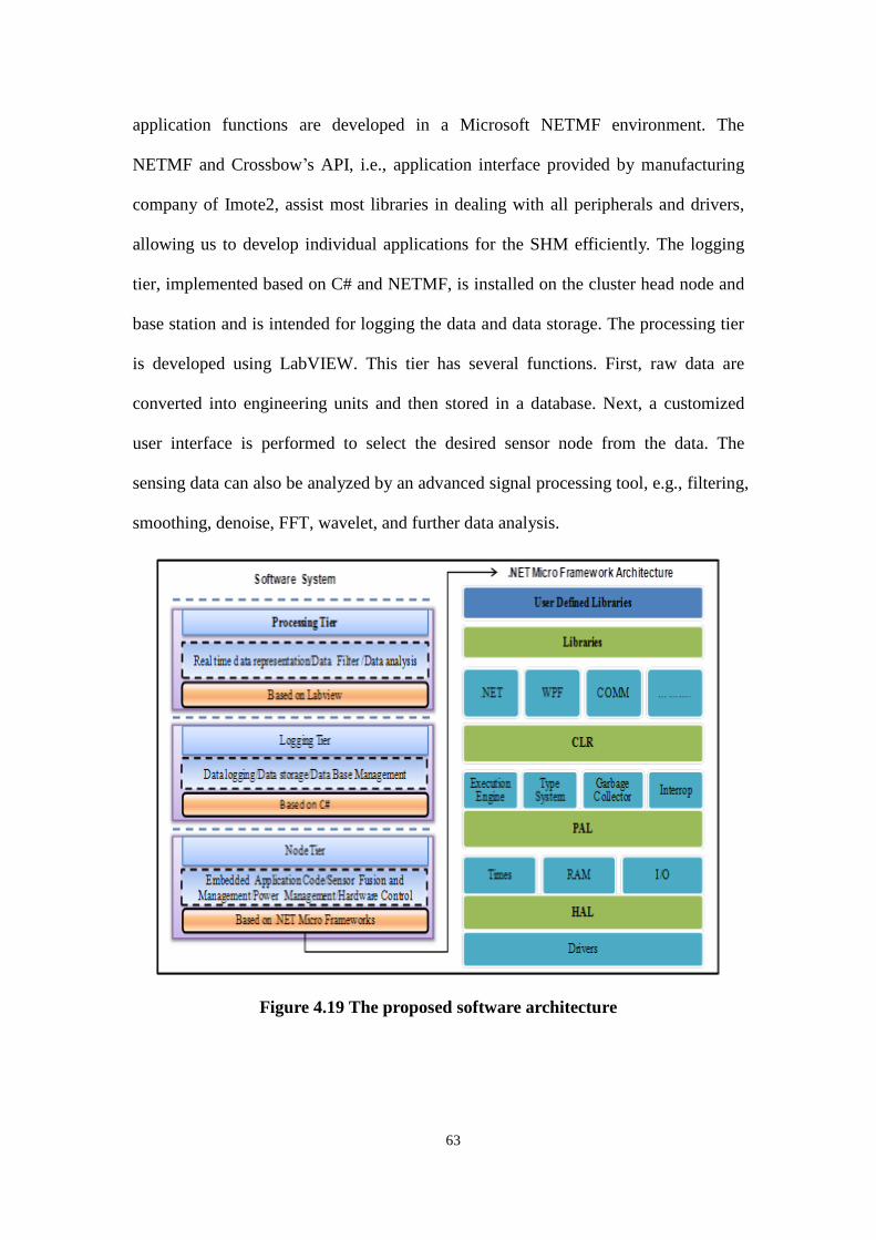
63

application functions are developed in a Microsoft NETMF environment. The

NETMF and Crossbow’s API, i.e., application interface provided by manufacturing

company of Imote2, assist most libraries in dealing with all peripherals and drivers,

allowing us to develop individual applications for the SHM efficiently. The logging

tier, implemented based on C# and NETMF, is installed on the cluster head node and

base station and is intended for logging the data and data storage. The processing tier

is developed using LabVIEW. This tier has several functions. First, raw data are

converted into engineering units and then stored in a database. Next, a customized

user interface is performed to select the desired sensor node from the data. The

sensing data can also be analyzed by an advanced signal processing tool, e.g., filtering,

smoothing, denoise, FFT, wavelet, and further data analysis.

Figure 4.19 The proposed software architecture

64

4.5.1 Net Micro Frameworks-Based Embedded Development

Environment

There are five layers in the basic architecture of NETMF. The platform

adaptation layer (PAL) and hardware abstraction layer (HAL) layer deal with the

hardware. The PAL supports higher-level integration, including asynchronous

communication calls, high-level timers, and list and data structures. The HAL

provides generic access to all peripherals and drivers. The NETMF’s common

language runtime (CLR) layer serves the purpose to load and execute managed code.

By supporting managed code, the NETMF CLR allows for rapid development and

safe execution of application code using modern programming languages and tools.

Microsoft developed several basic application libraries in library layer, and then

researchers can use it directly. As aforementioned description, the NET Micro

Framework help for dealing all peripherals and drivers, the developer hence can focus

on their individual application.

Figure 4.20 shows the structure of Class library which is branch out into three

basic class of NETMF, basic class library of Imote2, and SHM class. The SHM class,

a specialized class, is developed by this study for SHM application. Table4.6 gives a

description of these three classes. Based on these three classes, a SHM application for

specific purpose can be easily developed. Listing 4.1 presents an example code for

periodical deep sleep and sampling. For example, the radio can be initialized via the

constructor in Radio class: public Radio (ushort freq, ushort power, ushort

pan_address, ushort address) where define the frequency, power, node address,

and PAN address. After the parameters, such as the sampling rate, data types, and data

length are declared, the sampling starts remaining 60 s with a sampling rate of 200 Hz.

65

The sampling data then writing to a packet. After sampling, the packet is sent using

the Send method. Furthermore, for power saving, the mote can be put in deep sleep

mode (drawing 525 uA) for 60 s just call the DeepSleep method. Therefore, by using

above main functions and other fundamental APIs, the application can be developed

rapidly.

Figure 4.20 Structure of Class library

66

Table 4.6 Description of Class library

Namespace of class Name of class Description of class

Basic class of NETMF

Mscorlib A subset of the core .NET

classes.

System Only the System.Net

namespace

Microsoft.SPOT.Native Core .NET Micro

Framework classes.

Microsoft.SPOT.Hardware Managed hardware

drivers.

Microsoft.SPOT.Graphics Low-level graphics

classes.

Microsoft.SPOT.Net Internal socket drivers

basic class library of

Imote2

Platform For low-level access to the

mote hardware

Radio To set various radio

options

Sensors Various sensor drivers

Utilities Contains a number of

utility classes

SHM class

Extended math class Extend the basic math

class

Sampling Sampling the sensor data

Synchronization Synchronizing the nodes

FFT To calculate FFT

FRF To calculate FRF

67

Listing 4. 1. Sample code for periodical deep sleep and sampling

public class XAccel

{

public static void Main()

{

//Configurations

const ushort _rfChannel = (ushort)RadioChannel.Ch15; // channel 11

const ushort _rfPower = (ushort)RadioPower.M0DBM; // -10dbm

const int packet_length = 64;

const int packet2_length = 30;

Radio radio = new Radio(_rfChannel, _rfPower, 0xFFFF, 0xFFFF);

byte[] packet = new byte[packet_length];

byte[][] packetall = new byte[50000][];//

short accelX, accelY, accelZ; //accel raw values

int samplingrate = 5; //

samplepakage = 1200;// pakegets

int sendperiod = 50;

//Sampling

for (; ; )

{

while (pt < samplepakage)

{

accelX = (short)(accelX + _sensor.AccelXRaw);

accelY = (short)(accelY + _sensor.AccelYRaw);

accelZ = (short)(accelZ + _sensor.AccelZRaw);

packetall[row][index++] = (byte)(Av_x1 & 0xFF);

packetall[row][index++] = (byte)((Av_x1 >> 8) & 0xFF);

packetall[row][index++] = (byte)(Av_y1 & 0xFF);

packetall[row][index++] = (byte)((Av_y1 >> 8) & 0xFF);

packetall[row][index++] = (byte)(Av_z1 & 0xFF);

packetall[row][index++] = (byte)((Av_z1 >> 8) & 0xFF);

}

}

// sending data then go to deep sleep

radio.SetRadioOption(RadioOption.LocalAddress, (ushort)_nodeid);

for (row = 0; row < samplepakage; row++)

{

for (index = 4; index < packet_length; index++)

{

packet[index] = packetall[row][index];

}

packet[1] = (byte)row;

System.Threading.Thread.Sleep(sendperiod);

radio.Send((ushort)0xFFFF, (ushort)0xFFFF, packet);

}

pm.DeepSleep(600);

}

} //main

}

68

4.5.2 Data Logging and Data Storage

The logging tier, implemented based on C#, is installed on the cluster head node

and base station and is intended for logging the data and data storage. The data is

extracted from each packet and written to a text file or store in a database. The packet

carries three parts, which are TosMsg header, sensor board header and data payload

(Fig.4.21). The TosMsg header carries 5-byte TinyOS compatible header that provides

Imote2 protocol compatibility with MICA and IRIS motes. Table 4.7 Shows the

TosMsg header content. The next group in packet is the sensor board header that

provides basic information of node. Next are the data payload that includes all the

information serial number, timestamp, and sensor data. Herein, sensor data denotes 3

readings from X/Y/Z axis of the accelerometer sensor, each is 2 bytes. There are 10

groups in one packet. Table 4.8 and 4.9 present the content of sensor board header and

data payload.

Figure 4.21. Packet format

Table 4.7 TosMsg header contents

Type Field Name Description

uint16_t Address Destination address of the packet

uint8_t AM type TinyOS Active Message ID

uint8_t Group ID TinyOS group ID

uint8_t Length Length of the packet

TosMsg Header Sensor board header Data payload

Addres AM type Group ID Length

Serial number Timestamp Sensor data

Board_id Packet_id Node_id

TosMsg Header

Sensor board header

Data payload

69

Table 4.8 Sensor board header content

Type Field

Name Description

uint8_t board_id XSensor packet type field (Sensor streams are always a

constant value of 0x11)

uint8_t packet_id XSensor packet sub-type field (XAccel is always a constant

value of 0x01)

uint16_t node_id Network short address of sending node.

Table 4.9 Data payload

Type Field Name Description

uint16_t serial number Incrementing sequence number for yield calculation

uint16_t timestamp Timestamp information

uint16_t accel_x Accelerometer reading of X axis

uint16_t accel_y Accelerometer reading of Y axis

uint16_t accel_z Accelerometer reading of Z axis

…

uint16_t accel_x Accelerometer reading of X axis

uint16_t accel_y Accelerometer reading of Y axis

uint16_t accel_z Accelerometer reading of Z axis

4.5.3 User Interface and Visualized Signal Processing

The processing tier is developed using LabVIEW. This tier has several functions.

First, raw data are converted into engineering units and then stored in a database. Next,

a customized user interface is performed to select the desired sensor node from the

data. The sensing data can also be analyzed by an advanced signal processing tool,

e.g., filtering, smoothing, denoise, FFT, wavelet, and further data analysis. Figure

70

4.22 shows the functions of proposed user interface. Figure 4.23 shows how the

sensor data can be represented in a Figure. Chart and nodes distribution can also be

conveniently observed. Figure 4.25 presents the damage location in a visualization

window which can indicate the location of damage visibly.

Figure 4.22 Functions of proposed user interface

71

Figure 4.23 Sensor data representation and node distribution

Figure 4.24 Signal processing interface

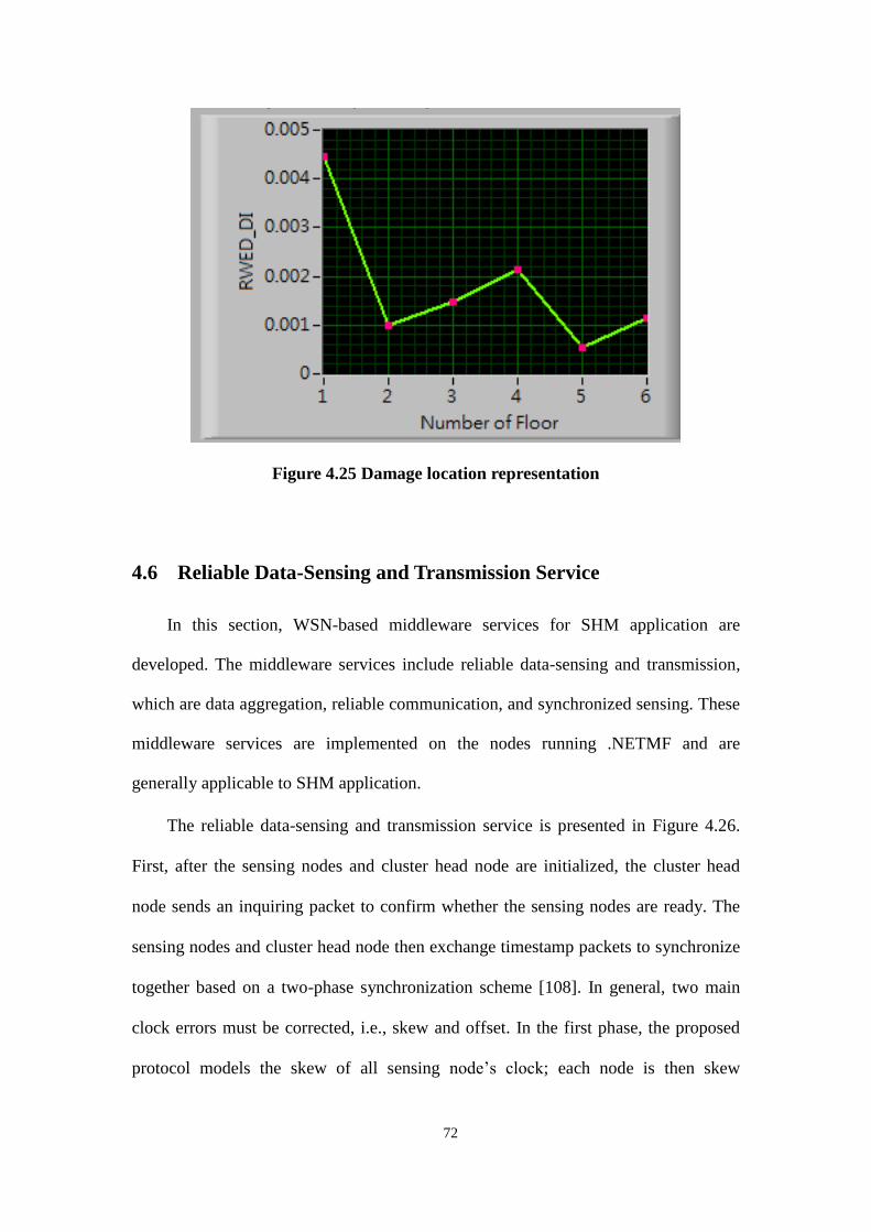
72

Figure 4.25 Damage location representation

4.6 Reliable Data-Sensing and Transmission Service

In this section, WSN-based middleware services for SHM application are

developed. The middleware services include reliable data-sensing and transmission,

which are data aggregation, reliable communication, and synchronized sensing. These

middleware services are implemented on the nodes running .NETMF and are

generally applicable to SHM application.

The reliable data-sensing and transmission service is presented in Figure 4.26.

First, after the sensing nodes and cluster head node are initialized, the cluster head

node sends an inquiring packet to confirm whether the sensing nodes are ready. The

sensing nodes and cluster head node then exchange timestamp packets to synchronize

together based on a two-phase synchronization scheme [108]. In general, two main

clock errors must be corrected, i.e., skew and offset. In the first phase, the proposed

protocol models the skew of all sensing node’s clock; each node is then skew

73

synchronized. Next, the skew is estimated by performing linear regression over

multiple timestamp packets from the cluster head node. Each timestamp packet Pi

contains the transmit timestamp ,B it obtained at the MAC level, just before the

packet leaves the cluster head node. The sensing nodes receive the packet at absolute

time ,B i B St D where B SD refers to the unknown propagation delay between the

cluster head node and the sensing nodes. The sensing nodes then record their local

time ,( ).S B i B SLT t D Although the local time includes the error due to clock skew

and offset in addition to propagation delay, the skew of the local clock can still be

modeled with respect to the reference clock of the cluster head node by performing

linear regression on the difference between ,B it and ,( ).S B i B SLT t D For N packets,

the clock skew can be modeled by linear regression over the data set of (xi,yi) pairs,

where xi and yi are , ,( ( ))B i S B i B St LT t D and ,( )S B i B SLT t D , respectively.

In the second phase, the clock offset is corrected by the classical two-way

synchronization exchange in a manner similar to that of the TPSN synchronization

protocol [115]. Once a sufficient number of packets to estimate the skew are obtained,

the sensing nodes send a packet with the skew-corrected local timestamp,

1 ( 1),ST LT T to the cluster head node. The cluster head node records its received

local time 2 ( 1 )B S BT LT T D , then replies with a packet to sensing nodes with T2

and transmit timestamp T3. Upon receiving the packet, the sensing nodes record the

skew-corrected local time 4 ( 3 ).S B ST LT T D Finally, the sensing node can

compute its clock offset as ( 2 1) ( 4 3) / 2Offset T T T T .

Following completion of the synchronization, all sensing nodes starts to sample

data and write data to an array. The parameters, such as the sampling rate, data type,

74

and data length, are declared before the sampling starts. Following the sampling, the

time-scheduling data transmission procedure is initiated to send data from the sensing

nodes to the cluster head node. Initially, the sensing nodes wait until a sending-delay

time is equivalent to (total sampling time + total packet sending time)* (node ID). For

instance, if the node ID is 0, the sensing node 0 transmits the packet immediately

since the sending-delay is zero. The data in each sensing node are then taken from the

array, filled in a packet, and sent to the cluster head node. With this procedure, each

node sequentially sends data to the cluster head node with a respective sending-delay

to avoid packet collision. However, packets losses occur occasionally, even though the

time-scheduling data transmission is designed to avoid packets collision. The base

station thus continuously checks the number of packets in the sequence from the

sensing nodes and records the number of each missing packet in the sequence. As a

result, the base station can request a sensor node to rectify the missed packets.

75

Figure 4.26. Reliable data-sensing and transmission service

Initializing

· Waiting for receiving packet form base station

Sensing node Cluster head node

Synchronization

· Skew estimation

· Compute its clock offset

· Correct clock

Inquiry

· Inquire of sensing nodes whether they are ready

Acknowledge

· Return acknowledge packet

Synchronization

· Exchange timestamp packet with sensing node

Parameters Declaration(E.g. sampling rate, data

type, data length, etc.)

Sampling dada

Write data to array

End of sampling

Yes

Take out data form array

Fill in packet

Send packet

End of Sending

Yes

Sampling

Time-scheduling data transmission

Waite sending-delay time

Sending-delay=(total sampling time + total

packet sending time)* (node ID)

No

No

Send missing data· Send missing packet to cluster head node

Receive data

· Receive and save data from sensing node

· Record the missing packets

Require missing data

· Send Request Packet for missing data

· Receive and save data from sensing node

Initializing

· Ready for sending commands

76

CHAPHER 5 DEVELOPMENT OF

GLOBAL-LOCAL-INTEGRATED DAMAGE

DETECTION APPROACH

5.1 Introduction

Structural health monitoring (SHM) was broadly classified into local and global

categories. The Non Destructive Testing (NDT) technique is mostly used in local

damage detection. There are many methods for NDE such as ultrasonic, infrared

thermography, eddy current X–ray. Such methods can detect tiny or incipient damage;

however, it is usually expensive, power hungry and bulky. Global SHM, on the other

hand, can discover damage large enough to influence the properties of the entire

structure or large sections of it. Most existing global damage detection methods

identified damage based on changes in basic modal properties that extract from

structural response by low cost sensing systems.

Both local and global SHM each has its own benefits and shortcoming, hence

integrating aforesaid two methods can obtain more effective damage detection result

than only using one of them. This research proposed a global-local-integrated damage

detection approach which is shown in Fig. 5.1.

77

Figure 5.1 global-local-integrated damage detection approach

In the first stage, the global method is adopted to detect the change of

characteristic of entire structure. Subsequently, roughly damage areas of structure are

Structure

Excitations

Sensing System

Response

Signal

processing

Global damage

detection

Local damage

identified

Roughly damage

Yes

No

Final estimation

• Ambient• Earthquake• Shaker• etc.

Building and Civil infrastructure

Integrated WSN SHM System

Substructure-based FRFapproaches

Electro-Mechanical-Impedance (EMI)-Based

damage detection method

78

identified. In stage two, after recognized the damage occurring and approximate

location, a local method was developed to identify the detailed condition of damage.

For instance, in a building structure, a global SHM can roughly indicate the location

of damaged floor. The local SHM then check the component of building structure in

detail. Substructure-based frequency response function approach was proposed as

global damage detection approach. Electro-Mechanical-Impedance (EMI)-Based

damage detection method is used to identify local damage of structure in this study.

5.2 Substructure-Based Frequency Response Function for Global

Damage Detection

A frequency response function (FRF) expresses the structural response to an

applied force as a function of frequency. This response may be represented in terms of

displacement, velocity, or acceleration [116, 117]. Theoretically, FRF can be

expressed in terms of system properties of mass, stiffness, damping, and modal

properties. Moreover, using measured FRF-data has a major benefit that the measured

FRF-data can provide much more damage information in a desired broadband

frequency range than modal data because the modal data are identified mainly from a

very limited number of FRF-data around resonance frequency [118, 119].Accordingly,

an FRF scheme is reasonably expected to be feasible for detecting structural damage.

Several studies have applied the FRF to locate damage. Thyagarajan et al. [120]

developed a method based on FRF data and an optimal number of sensors on a

structure to identify damage locations, overcoming the former limitation of large

number of computations required for high dof. structure. Lee and Shin[121] combined

an FRF-based structural damage identification method (SDIM) with a reduced domain

79

approach to detect damage to beam structures. This method depends on data for the

natural frequencies and mode shapes of the intact beams and the FRFs of damaged

beams to identify structural damage. They demonstrated the feasibility of this SDIM

using numerically simulated damage-identification tests. Their analytical results

illustrated that the use of FRFs seems to be very promising for structural damage

identification. Other investigations have extended FRF methods, such as the FRF

curvature method or the FRF shape-based method, to improve the detection of

damage locations. Sampaio et al.[122] developed a theoretical FRF curvature method

and evaluated the efficiency of this method using numerically simulated data and

experimental data for a real bridge. Their analytical results demonstrated that their

FRF curvature method was effective in detecting damage on single site. Maia et

al.[123] also presented an FRF curvature-based damage detection method and

compared its performance with that of a conventional mode shape-based method.

According to their results, methods based on FRF curvatures outperformed mode

shape-based methods. Liu et al.[124] developed an FRF shape-based method. This

method utilized the imaginary parts of FRF shapes of a beam structure to identify the

damage location before and after damage. Their analytical results exhibited that this

method was effective for a low-frequency range.

As well beam structures, FRF have been applied to detect damage in a building

structure. By using measured FRF and neural networks (NNs), Ni et al.[125]

identified the seismic damage of a 38-storey building model. That study determined

FRFs for dimensionality reduction and noise elimination based on principal

component analysis (PCA). According to their results, PCA is feasible for filtering

unwanted measurement noise. Their damage identified results obtained after moderate

earthquakes or super-strong earthquakes, in which considerable damage as identified

80

at the bottom portion of the building structure. Furukawa et al.[126] developed a

damage detection method using uncertain FRFs based on a statistical bootstrap

method and then applied it to a building structure. Their analytical results confirmed

that the proposed statistical method to detect structural damage can determine whether

the detected damage is a real damage or an identification error due to measurement

noise. Kanwar et al.[127] demonstrated the feasibility of using FRF to the structural

damage of reinforced concrete buildings. By using FRF, Hsu and Loh[128] detected

damage of building structure subjected to earthquake ground excitation. This method

required FRFs of intact and damaged systems as well as system matrices of the intact

system to derive the damage identification equations. Their numerical results

indicated that only the frequencies close to the natural frequencies of the damaged

system need to be selected in order to solve the identification equations. Meanwhile,

their experimental studies demonstrated the feasibility of the proposed algorithm in

detecting the structural damage within an acceptable accuracy.

Accordingly, an FRF scheme is reasonably expected to be feasible for detecting

structural damage. An novel substructure-based FRF approach with a damage location

index (SubFRFDI) was proposed to localize damage to building structures from

seismic response data.

5.2.1 Substructure-Based Frequency Response Function Approach

A frequency response function (FRF) is a transfer function, expressed in the

frequency domain. FRF can be represented in terms of magnitude and phase with real

and imaginary components. The response may be given in terms of displacement,

velocity, or acceleration. Consider a linear system as represented by the diagram in

Figure 5.2.

81

Figure 5.2 Frequency Response Function Model

The relationship in Figure 5.2 can be represented by the following equations

( )( )

( )

XH

F w

(5.1)

where the ( )F is the input force as a function of the angular frequency . ( )H is

the transfer function and ( )X is the displacement response function. Each function

is a complex spectral function, and considers each to be a Fourier transform for

simplicity.

Consider a SDOF system which was subjected to a force excitation and the basic

model of an SDOF system consists of a mass m, a spring with spring constant k, and a

damping coefficient c. The equation of motion is

( ) ( ) ( ) ( )mx t cx t kx t f t (5.2)

( )( ) ( ) ( )

c k f tx t x t x t

m m m (5.3)

By convention

22 ,n n

c k

m m (5.4)

where n is the natural frequency in (radians/sec), and is the damping ratio.

Transfer function

( )H

Input Force Displacement Response

( )F ( )X

82

By substituting Eq.(5.4) in to Eq. (5.3),

22 ( )

( ) 2 ( ) ( ) nn n

f tx t x t x t

k

(5.5)

Takes the Fourier transform of each side of equation (5.5), the resulting FRF is

2

2 2

( )

( ) ( (2 ))

n

n n

X

F w k j

(5.6)

where the n , k and are the nature frequency, stiffness and damping ration,

respectively. The defined FRF uses displacement as the response. It is known as

receptance.

By replacing the displacement response ( )X with velocity ( )X and

acceleration ( )X , two different types of FRFs cane be defined as:

2

2 2

( )

( ) ( (2 ))

n

n n

jX

F w k j

(5.7)

2 2

2 2

( )

( ) ( (2 ))

n

n n

X

F w k j

(5.8)

where the Eqs.5.7 and 5.8 are Mobility FRF and Accelerance FRF, respectively.

The reciprocals of the three FRFs of an SDOF system also have useful physical

significance and can be represented as

83

( )Dynamic stiffness =

( )

force F w

displacement X (5.9)

( )Mechanical impedance =

( )

force F w

velocity X (5.10)

( )Apparent mass =

( )

force F w

acceleration X (5.11)

In a shear building, beams and floor systems are assumed to be rigid in flexure.

Several factors, such as the axial deformation of beams and columns, and the effect of

axial force on column stiffness, are neglected in analysis. Although an ideal shear

building does not exist in practice, it is helpful for illustrating the use of

substructure-based FRF to locate damage. For a damped multi-degree of freedom

(MDOF) shear building with, say, N dofs., the equations of motion are

( ) ( ) ( ) ( )M x t C x t K x t f t

(5.12)

where M , C , and K are N N mass, viscous damping, and stiffness

matrices, respectively; and ( )x t and ( )f t are 1N vectors of the displacement

functions and effective external excitation load, respectively. The mass matrix is

diagonal, while C and K are tri-diagonal. Applying the Fourier transform to Eq.

(1) and performing a simple arrangement yields

1

2X K i C M F

(5.13)

which can be written simply as

84

( )

XH

F (5.14)

where ( )H is an FRF of the MDOF structure system as similar to the FRF

of SDOF system.

The MDOF structure is divided herein into various substructures. Consider an

N-storey shear building subjected to base excitations with acceleration ga , which can

be described by a simplified model (Fig. 5.3). N substructures of the original structure

can be easily established. The first substructure has the 1st—N

th dofs. while the second

has the 2nd—N

th dofs. Accordingly, the i

th substructure has the i

th—Nth

dofs. (Fig. 5.3).

The responses of any degrees of freedom of the ith

substructure are the same as those

of the original complete structure.

When 1i , considering an undamped sheer building model. For the ith

substructure, the balance of forces in the ith

floor can be written as

1 1 1( ) ( ) ( ( ) ( )) ( ) 0

i i i i i i i ik x t x t k x t x t m x t

(5.15)

where ( )ix t is the total displacement response of the ith

dof., and

( ) ( )i gx t x t a .

For the (i+1)th

to Nth

floors, the balance of forces is

1 1 2 2 1 1 1( ) ( ) ( ( ) ( )) ( ) 0


(5.16)

2 2 1 3 3 2 2 2( ) ( ) ( ( ) ( )) ( ) 0


(5.17)

85

1( ) ( ) ( ) 0

N N N N Nk x t x t m x t

(5.18)

The Eqs. (5.15’)~(5.18’) can be written as

1 1 1 1( ) ( ) ( ) ( ) ( )

i i i i i i i i ik k x t k x t m x t k x t

(5.19)

1 1 2 1 2 2 1 1( ) ( ) ( ) ( ) 0

i i i i i i i i ik x t k k x t k x m x t

(5.20)

2 1 2 3 2 3 3 2 2( ) ( ) ( ) ( ) 0

i i i i i i i i ik x t k k x t k x m x t

(5.21)

1( ) ( ) ( ) 0

N N N N N Nk x t k x t m x t

(5.22)

Equations (5.19’)~(5.22’) can be written as a matrix equation.

1 1

0 ( )

( )

0 ( )

i i

i i

N N

m x t

m x t

m x t

1 1 1

11 1 2 2

( ) ( )

0 ( ) 0

( )0 0

ii i i i i

ii i i i

N N

x tk k k k x t

x tk k k k

k x t

(5.23)

When damping is considered, Eq.(5.23’) can be expressed as

1 1

0 ( )

( )

0 ( )

i i

i i

N N

m x t

m x t

m x t

(5.24)

86

1 1

1 1 2 2 1

( )

0 ( )

0 ( )

i i i i

i i i i i

N N

c c c x t

c c c c x t

c x t

1 1 1 1

11 1 2 2

( ) ( ) ( )

0 ( ) 0

( )0 0

ii i i i i i i

ii i i i

N N

x tk k k c x t k x t

x tk k k k

k x t

where ( )ix t is the total displacement response of the ith

dof., and ( ) ( )i gx t x t a .

87

Figure 5.3. (a) Original complete structure, (b) the ith

substructure.

Equation (5.24) represents a single input/multiple output system. Clearly, the

substructure-based FRFs of the jth

dof. in the ith

substructure are

( )

1

( )( )

ji

j

i i i

XH

i c k X

, j = i to N (5.25)

where jX and 1iX are the Fourier transforms of ( )jx t and1( )ix t

, respectively. The

substructure-based FRF given by Eq. (5.25) depends on the properties of the ith—N

th

dofs. To estimate( ) ( )i

jH from Eq. (5.25), ic and ik must be known. Unfortunately,

(b)

xi-1(t)

mi

mi+1

mN

xi(t)

xi+1(t)

xN(t)

ki, ci

ki+1,ci+1

kN, cN

m1

mi-1

x1(t)

k1,c1

Feff(t)

xi-1(t)

mi

mi+1

mN

xi(t)

xi+1(t)

xN(t)

ki, ci

ki+1,ci+1

kN, cN

ith substructure

(a)

Original complete structure

ki-1, ci-1

88

ic and ik are usually unknown in the damage diagnosis process. Moreover,

acceleration responses are normally measured in monitoring the responses of a

structure in an earthquake. Therefore, the measured acceleration responses of the

original complete structure are used herein and these substructure-based FRFs are

further simplified as

( )

1

( )ji

j

i

XH

X

, j = i to N (5.26)

where jX and 1iX are the Fourier transforms of ( )jx t and 1( )ix t , respectively. A

specified substructure-based FRF,( ) ( )i

jH , can be estimated from measured

acceleration of the (i-1)th

and jth

dofs. Notably, when i =1, referring to the original

complete structural system, these substructure-based FRFs are given by

(1) ( )j

j

g

XH

A , j = 1 to N (5.27)

where gA is the Fourier transform of ga .

Theoretically, when the damage is assumed to have occurred in the column(s)

between the ith

and (i-1)th

dofs. (such that ki is reduced and ci is increased), the

substructure-based FRF is significantly altered in the ith

dof., as described by,

( ) ( )i

iH . Likewise, if stiffness ki and kl decline simultaneously, then the change in the

corresponding FRFs, ( ) ( )i

iH and( ) ( )l

lH , is greater than what would typically be

observed in ( ) ( )i

jH . Consequently, damage can be identified as having occurred at

89

a single or multiple sites. For efficiency, only one substructure-based FRF, ( ) ( )i

iH ,

is determined herein for each substructure to reduce the computational time. Damage

of the shearing building structures is located based on the FRFs,(1)

1 ( )H ,

(2)

2H , …, ( )N

NH , of all substructures.

Based on the aforementioned description, change in the substructure-based FRF

is related to damage and can be utilized as an essential index to locate damage of the

building structures. The operating conditions of this work are based on a known initial

state, continuously measured seismic response data, and comparisons of

before-and-after damage scenario for a shear building. Initially, sensors are deployed

on the shear building and the corresponding response data are measured immediately

after an earthquake excitation. The initial stiffness of the structure is then defined and

the corresponding FRFs

(1)

1, ( )uH ,(2)

2, ( )uH …,

( )

, ( )N

N uH are computed as a known

undamaged state, also referred to as a before-scenario state. Next, the sensors

continuously collect seismic response data of the structure after each subsequent

earthquake and the particular FRFs (1)

1, ( )dH ,(2)

2, ( )dH …,

( )

, ( )N

N dH are obtained

following, referred to as an after-scenario state. Before and after damage scenarios are

compared to determine the damage location since a change in the substructure-based

FRF is related to damage. A dissimilarity between the substructure-based FRFs in

damaged and undamaged states can be used to identify the damage. The absolute

dissimilarity ( )iP is defined as

90

( ) ( )

, ,( ) ( ) ( )i i

i i d i uP H H (5.28)

where ( )

, ( )i

i dH and ( )

, ( )i

i uH are the magnitudes of ( )i

iH in the damaged and

undamaged states, respectively. These N dissimilarities 1( )P — ( )NP can be

correspondingly calculated for a shear building with N floors. To locate conveniently

and quantify the damage, a substructure-based FRF damage location index

(SubFRFDI) for the ith

substructure is proposed. It is given by

221 ( ) /b

i i

a

SubFRFDI Exp NDF n

(5.29)

where , a, b, and n are working parameters and the ( )iNDF is expressed as

( ) ( )

, ,max max

( )( )

max ( ) , ( )

ii

i i

i d i u

PNDF

H H

(5.30)

The coefficient is a control value that scales the index between zero and one

and is set to five in this work. The range of selected frequencies for calculating

SubFRFDI is set to a—b, where a is a starting frequency of zero and b is the end

frequency, which equals the first modal frequency (undamaged state). The aforesaid a

and b are determined by trial-and-error method. The value n equals (b - a) divided by

sampling time, which is 0.005 s in this work. Figure 5.4 shows the FRF of

substructure.

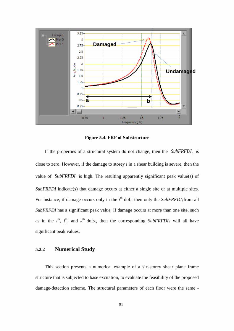
91

Figure 5.4. FRF of Substructure

If the properties of a structural system do not change, then the iSubFRFDI is

close to zero. However, if the damage to storey i in a shear building is severe, then the

value of iSubFRFDI is high. The resulting apparently significant peak value(s) of

SubFRFDI indicate(s) that damage occurs at either a single site or at multiple sites.

For instance, if damage occurs only in the ith

dof., then only the SubFRFDIi from all

SubFRFDI has a significant peak value. If damage occurs at more than one site, such

as in the ith

, jth

, and kth

dofs., then the corresponding SubFRFDIs will all have

significant peak values.

5.2.2 Numerical Study

This section presents a numerical example of a six-storey shear plane frame

structure that is subjected to base excitation, to evaluate the feasibility of the proposed

damage-detection scheme. The structural parameters of each floor were the same -

Damaged

Undamaged

a b

92

mass mi = 30 kg and stiffness ki = 55.5 kN/m (i = 1—6). Numerical simulation was

performed with 5% modal damping. The damage in this work was simulated as

reduced storey stiffness. Single-site and multiple-site damage were studied. Table 5.1

presents the simulated damage cases: Dam_ki (i = 1—6) denotes damage in the form

of reduced stiffness ki at a single site i; similarly, Dam_ki&kj (i ≠ j) represents

damages in the form of reduced stiffness ki and kj at multiple sites. Table 5.1 also

presents the percentage reduction in ki in parentheses.

Table 5.1 Descriptions of simulated damage cases.

Damage

case 1 2 3 4 5 6 7 8

Notation Dam_k1 Dam_k2 Dam_k3 Dam_k4 Dam_k1 Dam_k3 Dam_k3

&k5

Dam_k1

&k5

Damage

level k1 (15%) k2 (15%) k3 (15%) k4 (15%)

K1

(15%-30

%)

k3

(15%-30

%)

K3 (15%)

and

K5 (15%)

k1 (15%)

and k5

(15%)

Damage

case 9 10 11 12 13 14 15 16

Notation Dam_k1

&k3

Dam_k1

&k2

Dam_k1

&k2

Dam_k1

&k3

Dam_k1

&k3

Dam_k1

&k3&k5

Dam_k1

&k3&k5

Dam_k1

&k3&k5

Damage

level

k1 (15%)

and k3

(15%)

k1 (10%)

and

k2 (20%)

k1 (10%)

and

k2 (20%)

k1 (20%)

and

k3 (10%)

k1 (10%)

and

k3 (20%)

k1 (15%)

k3 (10%)

and k5

(5%)

k1 (5%)

k3 (15%)

and k5

(10%)

k1 (10%)

k3 (15%)

and k5 (5%)

For damage case 1, Figure 5.5 compares the conventional FRFs of the structure

in the undamaged and damaged states, while Fig. 5.6 compares the substructure-based

FRFs for each substructure. These Fig.s present only the parts of an FRF that

correspond to frequencies that are less than the second resonant frequency of the

complete structure or each substructure. The reduction in stiffness in the first storey

93

markedly changed the conventional FRFs of each floor whereas significant changes

were observed only in the substructure-based FRF of substructure 1. The

substructure-based FRF characterized and located damage more effectively than the

conventional FRF.

To apply the proposed substructure-based FRF approach to locate structural

damage, the locations of damage were determined using the SubFRFDI. Figure

5.7-5.10 presents the identified damage locations in four single-damage cases, 1, 2, 3,

and 4. When damage occurred only to the ith

storey, the value of the SubFRFDI that

corresponds to the ith

substructure greatly exceeded those that correspond to the other

substructures. The proposed index is verified to have located the damaged storey.

Four different percentage reductions in stiffness were assessed for damage case 1 and

3. Figure 5.11 and 5.12 shows the identified damage locations and corresponding to

damage extent. As shown in Fig., the damage can be correctly located and the value

of SubFRFDI was increasing corresponding to damage extent.

94

95

Figure 5.5 Comparisons of conventional FRFs of the structure in undamaged

and damaged states for Case 1.

96

97

Figure 5.6 Comparisons of the substructure-based FRFs for each substructure

for Case 1.

98

Figure 5.7 The identified damage locations in single-damage cases 1.


99



100

Figure 5.11 The identified damage locations in single-damage cases 1 for

different damage extent.

Figure 5.12 The identified damage locations in single-damage cases 3 for

different damage extent.

To study the effects of the frequency range in the SubFRFDIi, Fig. 5.13 presents

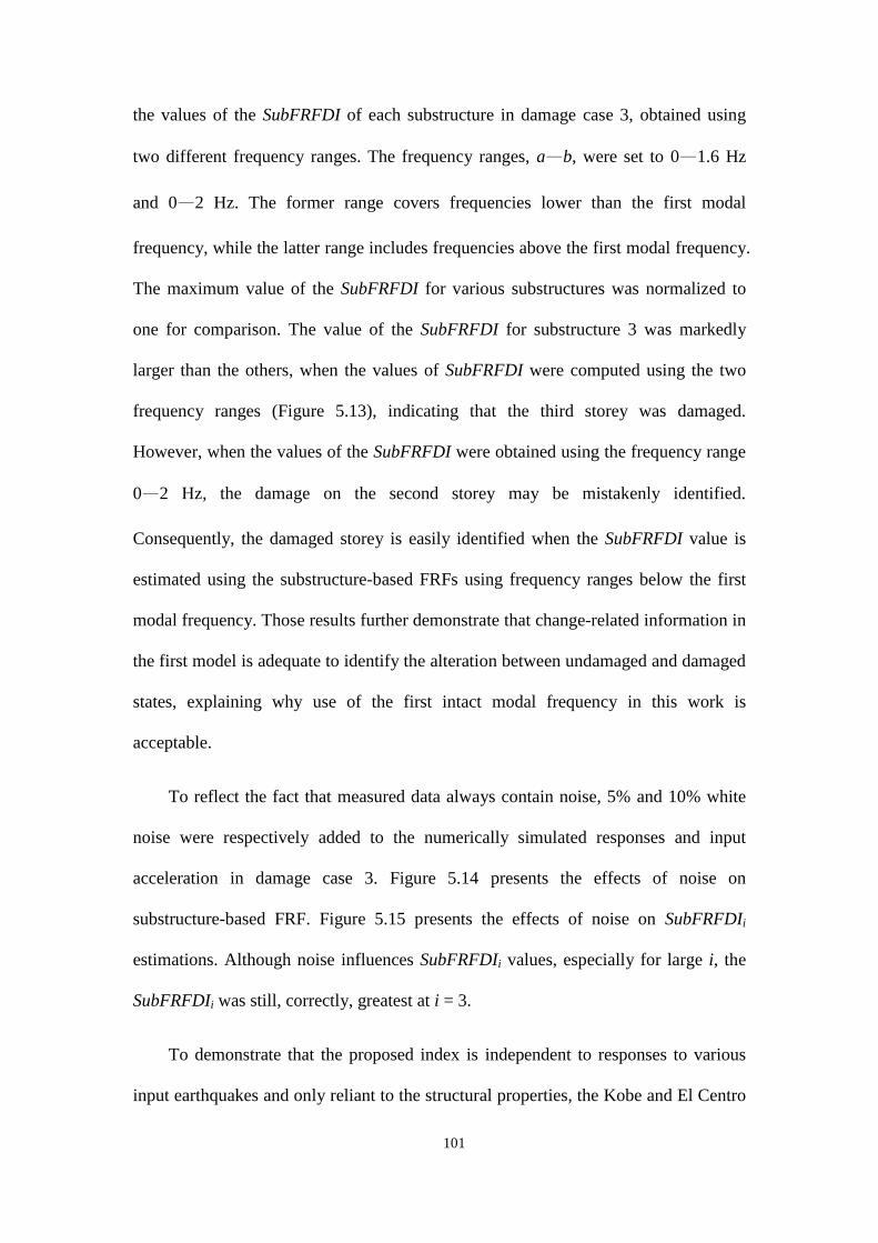
101

the values of the SubFRFDI of each substructure in damage case 3, obtained using

two different frequency ranges. The frequency ranges, a—b, were set to 0—1.6 Hz

and 0—2 Hz. The former range covers frequencies lower than the first modal

frequency, while the latter range includes frequencies above the first modal frequency.

The maximum value of the SubFRFDI for various substructures was normalized to

one for comparison. The value of the SubFRFDI for substructure 3 was markedly

larger than the others, when the values of SubFRFDI were computed using the two

frequency ranges (Figure 5.13), indicating that the third storey was damaged.

However, when the values of the SubFRFDI were obtained using the frequency range

0—2 Hz, the damage on the second storey may be mistakenly identified.

Consequently, the damaged storey is easily identified when the SubFRFDI value is

estimated using the substructure-based FRFs using frequency ranges below the first

modal frequency. Those results further demonstrate that change-related information in

the first model is adequate to identify the alteration between undamaged and damaged

states, explaining why use of the first intact modal frequency in this work is

acceptable.

To reflect the fact that measured data always contain noise, 5% and 10% white

noise were respectively added to the numerically simulated responses and input

acceleration in damage case 3. Figure 5.14 presents the effects of noise on

substructure-based FRF. Figure 5.15 presents the effects of noise on SubFRFDIi

estimations. Although noise influences SubFRFDIi values, especially for large i, the

SubFRFDIi was still, correctly, greatest at i = 3.

To demonstrate that the proposed index is independent to responses to various

input earthquakes and only reliant to the structural properties, the Kobe and El Centro

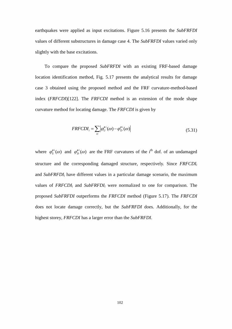
102

earthquakes were applied as input excitations. Figure 5.16 presents the SubFRFDI

values of different substructures in damage case 4. The SubFRFDI values varied only

slightly with the base excitations.

To compare the proposed SubFRFDI with an existing FRF-based damage

location identification method, Fig. 5.17 presents the analytical results for damage

case 3 obtained using the proposed method and the FRF curvature-method-based

index (FRFCDI)[122]. The FRFCDI method is an extension of the mode shape

curvature method for locating damage. The FRFCDI is given by

( ) ( )i i

i U DFRFCDI

(5.31)

where ( )i

U and ( )i

D are the FRF curvatures of the ith

dof. of an undamaged

structure and the corresponding damaged structure, respectively. Since FRFCDIi

and SubFRFDIi have different values in a particular damage scenario, the maximum

values of FRFCDIi and SubFRFDIi were normalized to one for comparison. The

proposed SubFRFDI outperforms the FRFCDI method (Figure 5.17). The FRFCDI

does not locate damage correctly, but the SubFRFDI does. Additionally, for the

highest storey, FRFCDI has a larger error than the SubFRFDI.

103

Figure 5.13 The values of the SubFRFDI of each substructure in damage case 3,

obtained using two different frequency ranges.

Figure 5.14. The FRF of substructure: With and without noise.

Number of Substructure

1 2 3 4 5 6

Norm

ali

ze S

ub

FR

FD

I

0.0

0.2

0.4

0.6

0.8

1.0

1.2

Chosen Range of

Frequency:0-1.6Hz

Chosen Range of

Frequency:0-2Hz

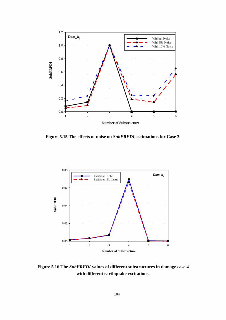
104

Figure 5.15 The effects of noise on SubFRFDIi estimations for Case 3.


1 2 3 4 5 6

Su

bF

RF

DI

0.00

0.02

0.04

0.06

0.08

Excitation_Kobe

Excitation_EL Centro

Dam_k4

Figure 5.16 The SubFRFDI values of different substructures in damage case 4

with different earthquake excitations.


1 2 3 4 5 6

Su

bF

RF

DI

0.0

0.2

0.4

0.6

0.8

1.0

1.2

Without Noise

With 5% Noise

With 10% Noise

Dam_k3

105


1 2 3 4 5 6

No

rma

lize

Su

bF

RF

DI

0.0

0.2

0.4

0.6

0.8

1.0

1.2

SubFRFDI

FRFCDI

Dam_k3

Figure 5.17 The analytical results for damage case 3 obtained using the proposed

method (SubFRFDI) and the FRF curvature-method-based index (FRFCDI).

The proposed approach can identify damage locations at multiple sites and a

single site. Figure 5.18-5.27 presents the SubFRFDI values for substructures in

damage cases 7—16. The corresponding peaks reveal that even though multiple

damage sites suffered damage of various degrees. Figures 5.18-5.27 present the

proposed index accurately determined the locations of the damage in a multi-damage

scenario.

106

Figure 5.18 The SubFRFDI values for substructures in damage cases 7, multiple

damage.


damage.

107

Figure 5.20. The SubFRFDI values for substructures in damage cases 9, multiple

damage.


damage.

108


damage.


damage.

109


damage.


damage with various damage level.

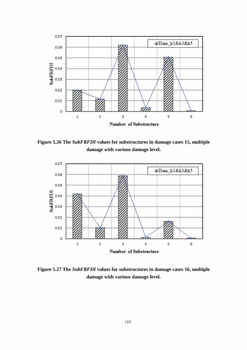
110





111

5.2.3 Implement of SubFRFDI in Integrated WSN-Based SHM

System

An SubFRFDI-based protocol was developed and embedded in the integrated

WSN-based SHM System. Figure 5.28 presents the SubFRFDI-based protocol when

using the WSN-based SHM System. Initially, the sensing nodes and base station

exchange timestamp packets so that they can be synchronized using a two-phase

synchronization scheme. The radio can be initialized via the constructor in Radio

class of C# where define the frequency, power, node address, and PAN address.

During the first phase, the proposed protocol models the skew in the clocks for all

sensing nodes; each node is then skew synchronized. Next, the skew is estimated by

performing linear regression over multiple timestamp packets from the base station.

After synchronization, the sensing node waits for the fire command from event node.

When the earthquake occurs, the event node immediately broadcasts a packet with a

fire command to the sensing nodes. To send and receive the packet is easily using the

classes Send and ReceiveAny. Finally, the sampling procedure for all sensing nodes

starts performing sampling data and writing data to a response array. Corresponding

parameters such as sampling rate, data type, and data length, are declared before

sampling starts.

After sampling, the FRF calculation procedure is initiated. The sensing node i-1

then send FFT data to sensing node i. The FFT data are written to an input array. The

FRF is next estimated by a FRF calculation function and is locally stored. Initially, the

FRF is estimated as a known undamaged state. After each subsequent earthquake, the

FRFs are referred to as a damage state. After the undamaged and damaged FRF are

obtained, the SubFRFDI can then be estimated in all sensing nodes. Finally, all

112

sensing nodes send their SubFRFDI to the base station to evaluate the damage to the

structure. In this protocol, the base station node and event node are powered by wall

plug to be always waking. The sensing nodes are powered by rechargeable battery

with energy harvesting system. All sensing nodes are set to be deep sleep mode and

waking up by turns. At least one sensing node is waking on each floor for ensuring

measuring. The mote can be put in deep sleep mode (drawing 525 uA) just call the

DeepSleep class for a specified period of time.

113

Figure 5.28 An SubFRFDI-based protocol

Initializing· Waiting for fire command from event node

Sensing node i

Parameters Declaration(E.g. sampling

rate, data type, data length, etc.)

Sampling dada

Write data to Response array

End of sampling

Yes

Sampling

No

FRF calculation

Estimate FFT using response array data

Receive FFT data from node i-1

Write data to input array

Estimate FRF=response /input

Calculate damage index

First time to

calculate FRF

Set FRF= ( )i

uH

Set FRF= ( )i

dH

Event trigger· Broadcast fire command to sensing nodes

Event node

Send index

· Send SubFRFDI to base station

Sensing node i-1

YES

NO

Synchronization· Skew estimation

· Compute its clock offset

· Correct clock

Synchronization

· Exchange timestamp packet with sensing node

Receive damage index

· Receive SubFRFDI from all sensing nodes

Base station

Control flow

Wireless communication between

nodes

221 ( ) /b

i i

a

SubFRFDI Exp NDF n

114

5.3 Electro-Mechanical-Impedance (EMI)-Based Local Damage

Detection Method

5.3.1 Fundamental of EMI-Based Model

The EMI based damage detection approach use the EM coupling effect between

active surface-bonded Piezoelectric patches and host structural. Researchers [64, 71]

showed that the EMI is related to the mechanical impedance of a host structure, thus

allowing monitoring the properties of the host structure using the measured electrical

impedance. A piezoelectric patch-structure bonded system can be modeled as a circuit

system [129], shown in Fig. 5.29. Herein, piezoelectric patch is modeled as a

capacitor (Cp) and a self sensing-actuation voltage source (Vp) caused by input

voltage (Vin). The output voltage, couple with Vp and Vin, can be expressed as

( )( ) ( ( ) ( ))

( ) ( )

Rout in p

R p

ZV V V

Z Z

(5.32)

where ZR is the electrical impedance of the resister and Zp is electrical impedance of

piezoelectric patch. Subsequently, the electrical impedance of piezoelectric patch can

be written as

( ) ( )( ) ( ) 1

( )

in p

p R

out

V VZ Z

V

(5.33)

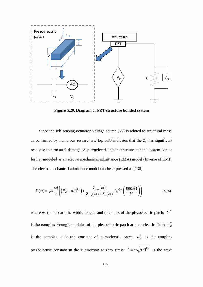
115

Figure 5.29. Diagram of PZT-structure bonded system

Since the self sensing-actuation voltage source (Vp) is related to structural mass,

as confirmed by numerous researchers. Eq. 5.33 indicates that the Zp has significant

response to structural damage. A piezoelectric patch-structure bonded system can be

further modeled as an electro mechanical admittance (EMA) model (Inverse of EMI).

The electro mechanical admittance model can be expressed as [130]

2 2

33 31 31

tan( )ˆ ˆ( )pmT E E

pm s

Zwl klY j d Y d Y

t Z Z kl

(5.34)

where w, l, and t are the width, length, and thickness of the piezoelectric patch; ˆ EY

is the complex Young’s modulus of the piezoelectric patch at zero electric field; 33

T

is the complex dielectric constant of piezoelectric patch; 2

31d is the coupling

piezoelectric constant in the x direction at zero stress; ˆ/ Ek Y is the wave

structure

PZT

Vin VoutR

VpCp

AC

V

12

3

w

l

t

Piezoelectric patch

116

number that is related to mass density , ˆ EY ; and excitation frequency ,

respectively; pmZ and sZ are the mechanical impedances of the piezoelectric patch

and the host structure, respectively. For a SDOF structure system, the mechanical

impedances of structure is defined as

0 i

s s

FZ Z e

(5.35)

in which

2

2

2s

m kZ c

(5.36)

where the 0F is a harmonic excitation force at angular frequency ; is velocity

response in frequency domain; the m, c and k are mass, damping and stiffness of

structure, respectively.

Equation (5.34) indicates that the EMI (or EMA) is directly related to the

mechanical impedance of structure. As described in Eq. (5.34) and Eq. (5.35), when

damage occurred to structure, the mechanical impedance of structure will be changed.

Therefore, if the mechanical impedances of the piezoelectric patch remain undamaged,

any changes in the EMI signal correlates with the damage in structure.

Although the EMI provides a qualitative method for detecting structural damage,

the quantification approach need be established. A simple statistical algorithm, which

is based on frequency-by-frequency comparisons, referred to Root Mean Square

Deviation (RMSD), was used to develop the quantitative assessment of damage in

previous research [69, 129, 131]. The RMSD is defined as

117

2

2100

bD U

i i

i a

bU

i

i a

I I

RMSD

I

(5.37)

where U

iI and D

iI are the real part of impedance of piezoelectric patch at the ith

frequency point in undamaged and damaged structures, respectively. In a RMSD

damage metric chart, the greater numerical value of the metric, the larger the

difference between the baseline reading and the subsequent reading indicates the

presence of damage in a structure.

5.3.2 Measurement of Piezoelectric-Impedance

The measurement of piezoelectric impedance is typically implemented by an

impedance analyzer. The disadvantages of using impedance analyzer are relatively

bulky size, expensive, and no portable. The Peairs et al. [132] developed an effective

device using a digital signal analyzer with an FFT function that can measure and

record the electric impedance of a PZT. Advantages of the new impedance-measuring

device include its low cost, greater accessibility, and smaller size.

Credit to the progress of Micro Electronic Mechanical System (MEMS), the new

single-chip impedance measurement device, AD5933 has been developed by Analog

Device Inc. The AD5933 is a high precision impedance measurement device that

combines an on-board frequency generator with a 12-bit, 1 MSPS, analog-to-digital

converter (ADC). The frequency generator allows exciting external complex

impedance with a known frequency. The response signal from the impedance is

sampled by the on-board ADC and a discrete Fourier transform (DFT) is processed by

an on-board DSP engine. The DFT algorithm returns a real (R) and imaginary (I)

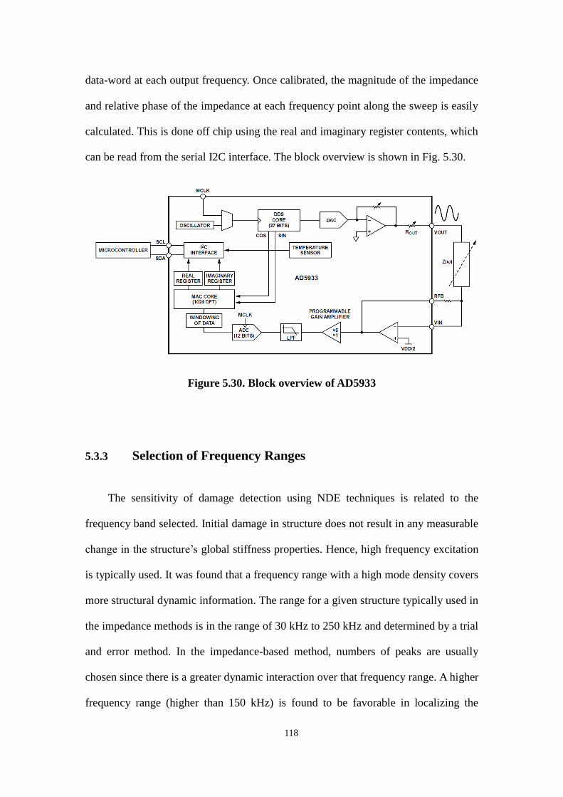
118

data-word at each output frequency. Once calibrated, the magnitude of the impedance

and relative phase of the impedance at each frequency point along the sweep is easily

calculated. This is done off chip using the real and imaginary register contents, which

can be read from the serial I2C interface. The block overview is shown in Fig. 5.30.

Figure 5.30. Block overview of AD5933

5.3.3 Selection of Frequency Ranges

The sensitivity of damage detection using NDE techniques is related to the

frequency band selected. Initial damage in structure does not result in any measurable

change in the structure’s global stiffness properties. Hence, high frequency excitation

is typically used. It was found that a frequency range with a high mode density covers

more structural dynamic information. The range for a given structure typically used in

the impedance methods is in the range of 30 kHz to 250 kHz and determined by a trial

and error method. In the impedance-based method, numbers of peaks are usually

chosen since there is a greater dynamic interaction over that frequency range. A higher

frequency range (higher than 150 kHz) is found to be favorable in localizing the

119

sensing, while a lower frequency range (lower than 70 kHz) covers more sensing

areas. [71, 131, 133].

Under the high frequency ranges used in this impedance-based method, the

sensing region of the piezoelectric patch is localized to a region close to the

sensor/actuator. Through various case studies in Esteban’s work [134], it has been

estimated that (depending on the material and density of the structure) the sensing

area of a single PZT can vary anywhere from 0.4 m (sensing radius) on composite

reinforced concrete structures, to 2 m on simple metal beams. The frequency ranges

higher than 500 kHz have been found to be unfavorable, because the sensing region

becomes extremely small and the PZT sensors show adverse sensitivity to their

bonding conditions or PZT itself rather than behavior of a structure monitored.

120

CHAPHER 6 EXPERIMENTAL VERIFICATION

6.1 Introduction

In this chapter, this dissertation focused on the experimental study. When the

theoretical basis of damage detection method and wireless SHM system based

measuring system are completed, series experimental study are conducted to verify

the proposed algorithm and system. First off all, the integrated WSN-based SHM

system is verified involving sensor calibration, wireless communication quality, data

losing, interference in material, power consumption. Subsequently, the proposed

damage detection approach with proposed SHM system then investigated in a ¼ -scale

six-storey steel structure that was designed by the National Center for Research on

Earthquake Engineering (NCREE), Taiwan. Subsequently, the proposed wireless

SHM system is employed in a bridge structure to test the feasibility in field.

6.2 Verification of Integrated WSN-Based SHM System

6.2.1 Verification of Sensing Node

In this test, the reliable data-sensing and transmission service is implemented on

the sensing node and cluster head node. The sensing capability is calibrated compared

to reference wire sensor. Two sensing nodes and a reference wire sensor (CXL01LF1)

are attached on a Quanser shaking table to measure acceleration of table. The shaking

table is excited by controller using Sin wave excitation input. Two sensing node and

reference sensor are installed next to each other and the corresponding signals from

those are expected to be identical. Measured dynamic responses were acquired by

121

sensing nodes and sent to the cluster head node connected to a host computer. Figure

6.1 compares the acceleration time history measured by two sensing nodes and

reference sensor. The time history schemes of the wireless sensing nodes and

reference sensor have identical shapes and magnitudes. This confirms good-quality

data collection by the wireless sensing system. The same observation is made when

the signals are compared in terms of FFT (Fig. 6.2) and power spectral density (Fig.

6.3). Moreover, the peak of FFT indicates the wireless sensing node can identify the

shaking table is moving on 2 Hz Sin wave.

Figure 6.1 Acceleration record from wireless sensing nodes and reference sensor.

122

Figure 6.2 FFT of acceleration record from wireless sensing nodes and reference

sensor.

Figure 6.3 Power spectral density of acceleration record from wireless sensing

nodes and reference sensor.

Frequency(Hz)

0 1 2 3 4 5

Am

p.

0.00

0.02

0.04

0.06

0.08

0.10

0.12

0.14

Reference sensor

Wireless sensing node1


2D Graph 8

Frequency(Hz)

0 5 10 15 20 25 30

db

-140

-120

-100

-80

-60

-40

-20

0

Reference sensor



123

This experimental study then evaluated the feasibility and robustness of the

proposed system in a 1/8-scaled three-storey steel frame model (Fig.6.4) was

employed to verify the performance of the wireless sensing system placed on a

Quanser shaking table. Each floor weighed about 3.8 kg and each column had a

cross-sectional area of 80 mm2 and was 440 mm in height. Wireless sensing nodes

were deployed at the center of each floor. In this test, the model was excited by the

Quanser shaking table using earthquake time history excitation data. The

measurement period was 60 sec, during which data were oversampled. Oversampling,

typically used for anti-aliasing, was based on the Nyquist theorem. Measurement data

were sampled at 800Hz, and then down-sampled to a sampling rate of 200 Hz.

Measured structural dynamic responses were acquired by sensing nodes and sent to

the cluster head node connected to a host computer. Figure 6.5 shows the ground

acceleration time history measured by wireless sensing nodes. Following, acceleration

measurements from the wireless sensors identified natural frequencies by applying an

ANN-based system identification (ANNSI) model [46]. The corresponding first three

natural frequencies of the structure were 1.83, 5.42, and 7.96Hz. The modal

parameters can be considered reasonable by comparing to FEM model.

124

Figure 6.4 A 1/8-scaled three-storey steel frame model.

125

0 10 20 305 15 25

Time(sec)

-1

-0.6

-0.2

0.2

0.6

1

Acc

eler

atio

n(g)

input excitation

-1

-0.6

-0.2

0.2

0.6

1

Acc

eler

atio

n(g)

1st floor

-1

-0.6

-0.2

0.2

0.6

1

Acc

eler

atio

n(g)

2nd floor

-1

-0.6

-0.2

0.2

0.6

1

Acc

eler

atio

n(g)

3rd floor

Figure 6.5 Acceleration record from wireless sensing nodes

126

4 8 126 10 14

Time(s)

-1

-0.6

-0.2

0.2

0.6

1

no

malize

d r

esp

on

ses

1st floor

wireless

ANN

-1

-0.6

-0.2

0.2

0.6

1

no

malized

resp

on

ses

2nd floor

wireless

ANN

-1

-0.6

-0.2

0.2

0.6

1

no

malized

resp

on

ses

3rd floor

wireless

ANN

Figure 6.6. Response for ANN and wireless sensor node

127

6.2.2 Reliability of RF Communication Test

In a WSN, some packets may be lost during the RF communication. For instance,

packets may collide with each other if multiple nodes attempt to send packets to the

base station simultaneously. Packet loss may thus cause incomplete measurement

signals. Herein, the successful packet received rate (SPRR) was utilized to evaluate

the reliability of data transmission among nodes. The SPRR is defined as the number

of successfully received packets divided by the number of sent packets. In practice,

sensing nodes send a fixed number of packets to a base station. The base station can

thus calculate the SPRR by using the number of sent and received packets.

The SPRR was used to evaluate the packet sent interval. In this study, the packet

sent interval was 20 ms when the value of SPRR approached 1.0 whereas the SPRR

declined as the packet sent interval decreased during the wireless communication test.

In SHM, extended period measurement is necessary. In contrast with the

conventionally adopted wired sensor system, the wireless sensor node runs an

individual procedure on its CPU, with any exception event possibly disrupting node

operations. Therefore, the stability and robustness for extended period measurement

should be assessed. The measured period was set as 10, 30, 60 and 120 minutes,

respectively. The sampling rate was 200Hz. The sensor nodes sample and transmit

data to the base station via the proposed reliable data-sensing and transmission service.

The base station then calculates the SPRR for data loss evaluation. Figure 6.7

indicates that the average SPRR is almost 99% for 10, 30, 60 and 120 minutes. This

indicates that data loss was lower than 1% even in extended measuring period. It

means that the proposed system is robust and stable for long term monitoring.

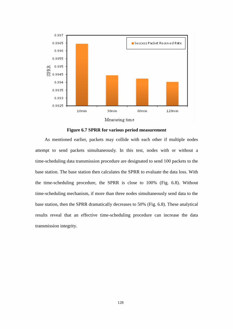
128

Figure 6.7 SPRR for various period measurement

As mentioned earlier, packets may collide with each other if multiple nodes

attempt to send packets simultaneously. In this test, nodes with or without a

time-scheduling data transmission procedure are designated to send 100 packets to the

base station. The base station then calculates the SPRR to evaluate the data loss. With

the time-scheduling procedure, the SPRR is close to 100% (Fig. 6.8). Without

time-scheduling mechanism, if more than three nodes simultaneously send data to the

base station, then the SPRR dramatically decreases to 50% (Fig. 6.8). These analytical

results reveal that an effective time-scheduling procedure can increase the data

transmission integrity.

129

Figure 6.8 Comparison of success packets received rate(SPRR) for well Time

Schedule and Non Time Schedule.

Figure 6.9 presents the relation between RF power and distance and the SPRR.

Clearly, transmission range depends on RF power. A higher power output increases

range but also increases power consumption. Therefore, Figure 6.9 is a useful

reference when deploying the sensor nodes in the structure. Each node can be

allocated a different transmission power to optimize power consumption for varying

distance. In the experimental study, the farthest distance was 20m. Hence, power was

set to -15dbm to reduce power consumption.

130

Figure 6.9. Successful packet received rate (SPRR) to RF Power and Distance

6.2.3 Field Test in Bridge Structure

In Taiwan, the typhoon cause great damage on bridge due to Bridge Scour.

Hence, the monitoring of Bridge Scour has received considerable interest in the last

decade. Traditional site investigation methods are expensive and time-consuming and

may not always give a complete assessment. Geophysical methods can be used to

determine the riverbed profile below the water in a river. A trial of ground penetrating

radar (GPR) is a geophysical method that is particularly efficient in determining the

sub-bottom geological structure in a shallow freshwater environment. Forde et al.

[135] discussed a number of scour surveys using GPR. They concluded that GPR

131

surveys can be effective in determining both the water depth and sub-bottom

geological structure near bridge piers and abutments. Yankielun et al. [136] conducted

a laboratory experiment using time-domain reflectometry (TDR) for monitoring scour.

Their system capable of continuous round-the-clock operation can be used to

constantly monitor the extent of scour and can indicate changes in sediment depth of

less than 5 cm. The fiber Bragg grating (FBG) was also an alternative technique for

scour monitoring. Lin et al. [137] developed a FBG based monitoring system and

tested in the laboratory. Their FBG scour-monitoring systems can be used to measure

both the processes of scouring/deposition and the variations of water level. Several

experimental runs have been conducted in the scaled flume to demonstrate the

applicability of the system. Their experimental results indicate that the real-time FBG

monitoring system has the potential monitor the scour. However, further applications

in the field should be conducted. The robotic system was also presented for

underwater inspection of bridge substructures. DeVault [138] developed an automated

robotic system for underwater inspection of bridge substructures. This robotic system

can detect scour, deterioration, or damage to support columns by two identical mobile

robots designed to travel along opposite surfaces of the pier while connected to each

another by a cable and winch system. It provides positional data and sensor

information (video images) to the system operator for condition evaluation.

The conventional wired sensing system is expensive and infeasible.

Characterized by its low manufacturing costs, low power requirements, miniaturized

size, and no need for cabling, the wireless sensor networks (WSN) is an attractive

sensing technology for deploying sensors for bridge scour monitoring. Hence, the

developed integrated WSN-based SHM system was deployed in a bridge to test the

feasibility and practicality in real civil structure.

132

The proposed system was deploying in Nioudou Bridge. A field free vibration

test was conducted for obtaining dynamic response. Two piers were connected by a

steel bar for free vibration test. The soil ground was excavated to 4m depth to

simulate scouring. The free vibration test was performed twice for comparing intact

and scouring case. Dynamic responses were record and send to base station via

data-sensing and transmission service from wireless sensing nodes.

6.2.3.1 Experimental Setup

Figure 6.10 presents the experiment setup and sensor locations. The field

experiment was conducted in Nioudou Bridge. Two piers were connected by a steel

bar for a free vibration test. Hydraulic machinery was used to provide a tensile force

on the steel bar. The tensile force was increasing till the weak part of the steel bar was

broken. This broken energy forces the pier for free vibration. The maximum tensile

force was previously examined by a Tensile Test in the laboratory. Figure 6.11 shows

the maximum tensile force is 250kN. Three wireless sensing nodes were deployed on

the top, center and bottom of the pier 1(P1), respectively. Dynamic responses were

record and send to base station via reliable data-sensing and transmission service. The

soil ground was excavated to 4m depth to simulate scouring. The free vibration test

was performed twice for comparing intact and scouring case.

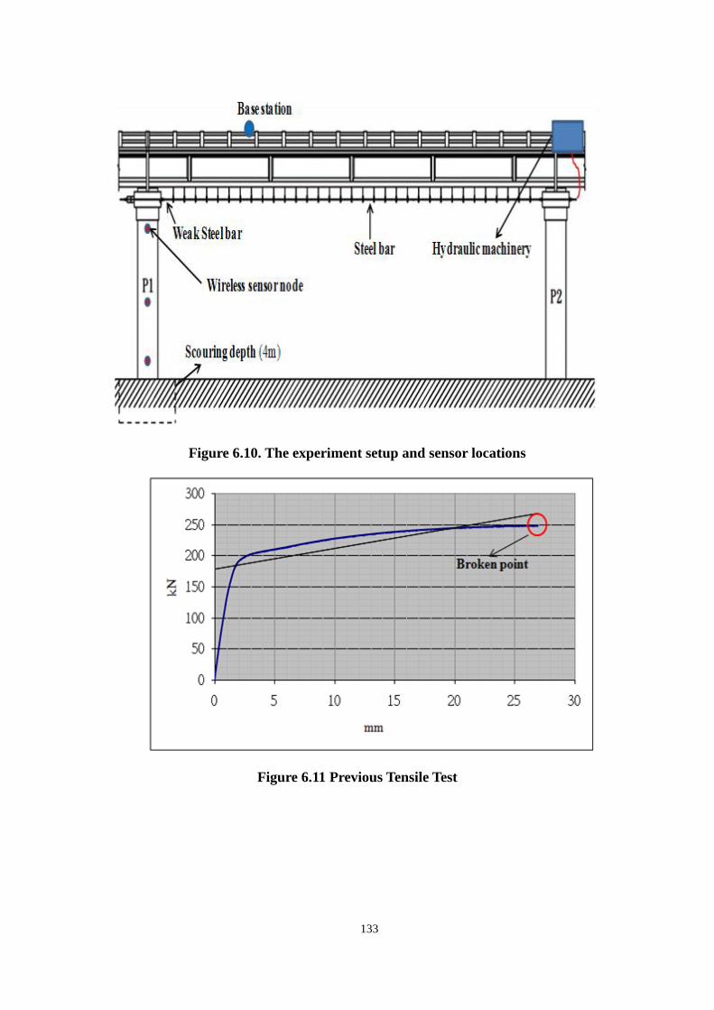
133

Figure 6.10. The experiment setup and sensor locations

Figure 6.11 Previous Tensile Test

134

6.2.3.2 Experimental Results

Figure 6.12-6.15 shows the photograph of field experiment. Figure 6.12 shows

the Nioudou Bridge. The expansion joint was previously removed to increase the

displacement of pier when perform free vibration test. Figure 6.13 shows the weak

part of the steel bar. Two weak steel bars were used in intact and scouring case. The

steel bars were broken when the tensile force reach 180kN and 220kN respectively in

intact and scouring case. Figure 6.14 demonstrates the excavation condition to

simulate scouring. Figure 6.15 presents the location of wireless sensing node which is

fixed in the pier.

Figure 6.12 Photo of Nioudou Bridge

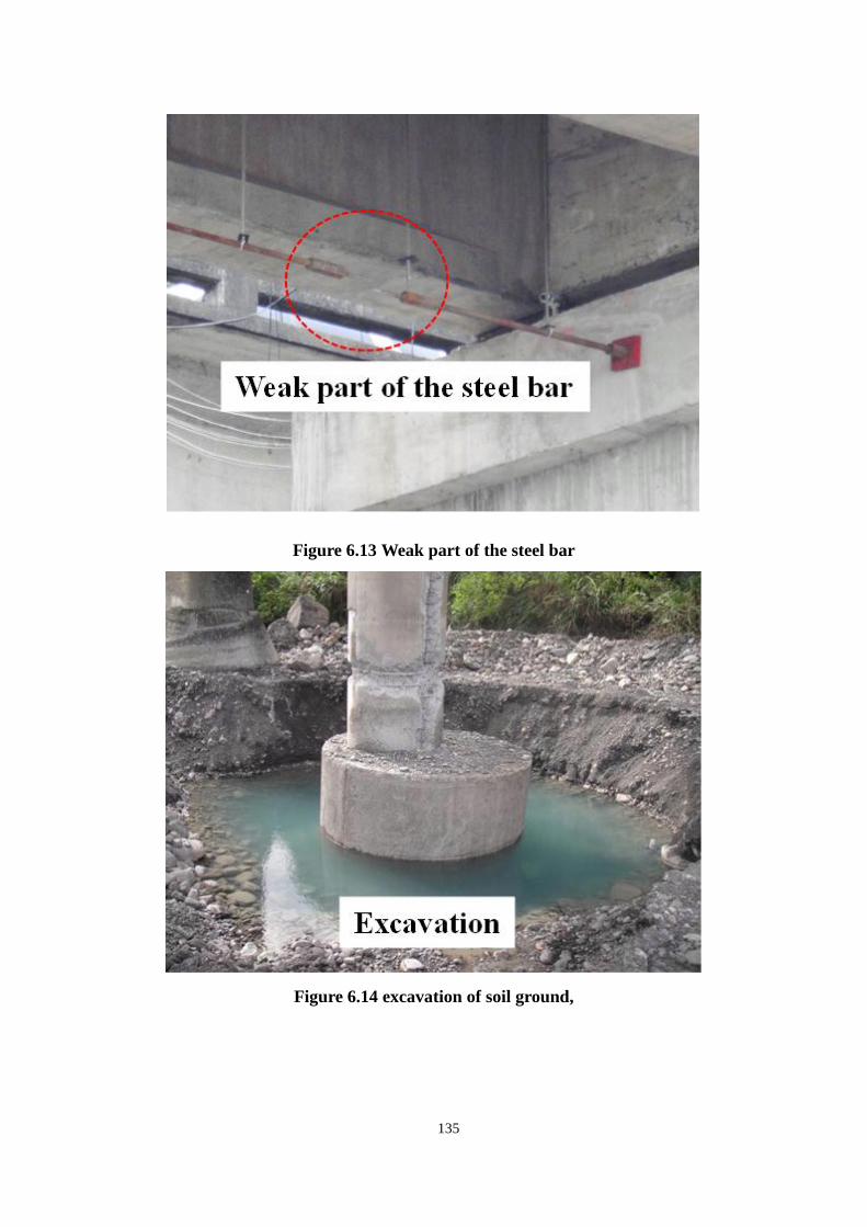
135

Figure 6.13 Weak part of the steel bar

Figure 6.14 excavation of soil ground,

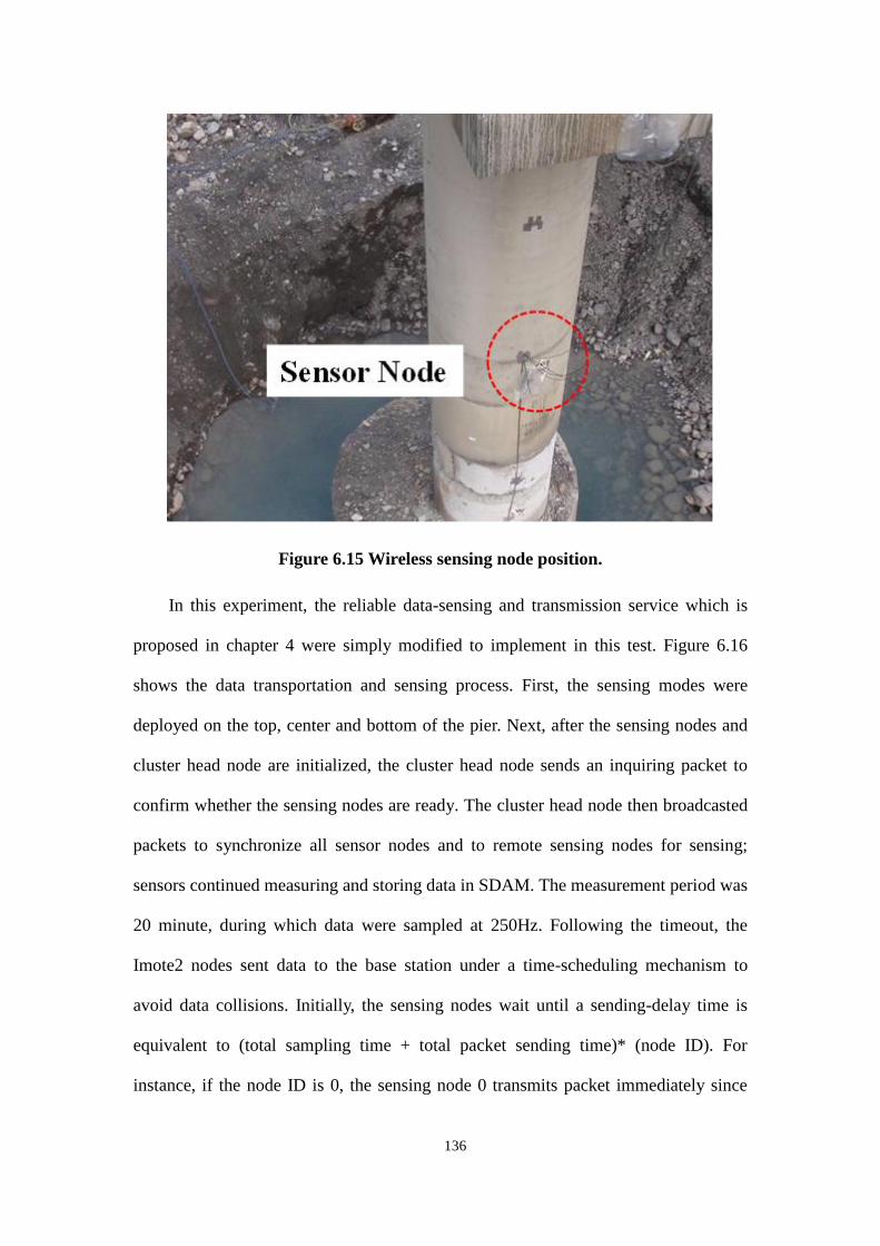
136

Figure 6.15 Wireless sensing node position.

In this experiment, the reliable data-sensing and transmission service which is

proposed in chapter 4 were simply modified to implement in this test. Figure 6.16

shows the data transportation and sensing process. First, the sensing modes were

deployed on the top, center and bottom of the pier. Next, after the sensing nodes and

cluster head node are initialized, the cluster head node sends an inquiring packet to

confirm whether the sensing nodes are ready. The cluster head node then broadcasted

packets to synchronize all sensor nodes and to remote sensing nodes for sensing;

sensors continued measuring and storing data in SDAM. The measurement period was

20 minute, during which data were sampled at 250Hz. Following the timeout, the

Imote2 nodes sent data to the base station under a time-scheduling mechanism to

avoid data collisions. Initially, the sensing nodes wait until a sending-delay time is

equivalent to (total sampling time + total packet sending time)* (node ID). For

instance, if the node ID is 0, the sensing node 0 transmits packet immediately since

137

the sending-delay equals zero. The data in each sensing node are then taken from the

array, filled in a packet, and sent to the base station. Based on this procedure, each

node sequentially sends the data to the base station with a respective sending-delay,

which can avoid the packet collision.

Figure 6.16 Modified reliable data-sensing and transmission service

138

Figure 6.17 shows the acceleration response measured by the sensing nodes. The

good-quality data collection by the wireless sensing system successfully records a

typical free vibration response of the pier. Figure 6.18 shows the responses on the top

sensing node for comparing the intact and scouring case. Observing to the response of

the free vibration, it indicates that the free vibration response for intact tend to stable

faster than the scouring case. Figure 6.19 compares two FFTs for intact and scouring

case. In frequency domain, the difference between intact and scouring case can be

observed. The work indicates that the proposed wireless sensing system was a reliable

technology for monitoring bridge structure.

Figure 6.17 Responses of sensor nodes for intact case.

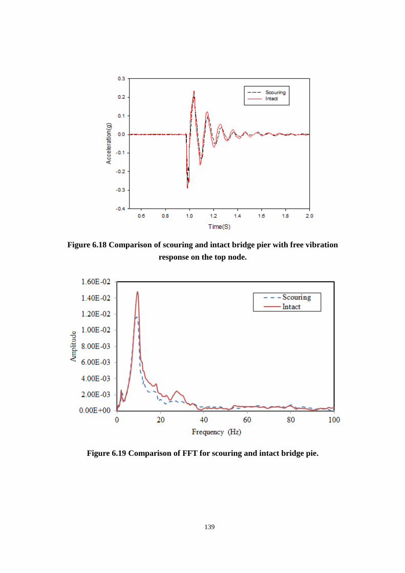
139

Figure 6.18 Comparison of scouring and intact bridge pier with free vibration

response on the top node.

Figure 6.19 Comparison of FFT for scouring and intact bridge pie.

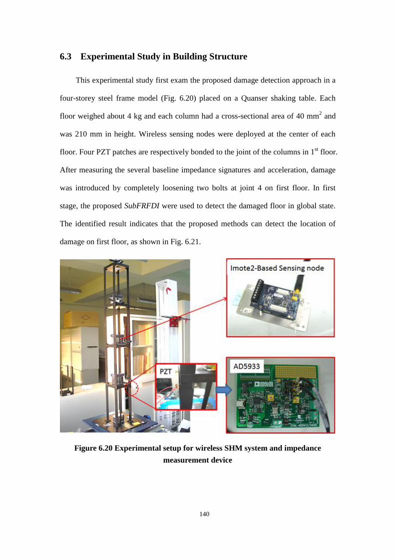
140

6.3 Experimental Study in Building Structure

This experimental study first exam the proposed damage detection approach in a

four-storey steel frame model (Fig. 6.20) placed on a Quanser shaking table. Each

floor weighed about 4 kg and each column had a cross-sectional area of 40 mm2 and

was 210 mm in height. Wireless sensing nodes were deployed at the center of each

floor. Four PZT patches are respectively bonded to the joint of the columns in 1st floor.

After measuring the several baseline impedance signatures and acceleration, damage

was introduced by completely loosening two bolts at joint 4 on first floor. In first

stage, the proposed SubFRFDI were used to detect the damaged floor in global state.

The identified result indicates that the proposed methods can detect the location of

damage on first floor, as shown in Fig. 6.21.

Figure 6.20 Experimental setup for wireless SHM system and impedance

measurement device

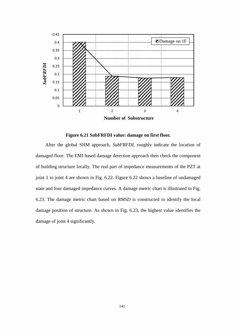
141

Figure 6.21 SubFRFDI value: damage on first floor.

After the global SHM approach, SubFRFDI, roughly indicate the location of

damaged floor. The EMI based damage detection approach then check the component

of building structure locally. The real part of impedance measurements of the PZT at

joint 1 to joint 4 are shown in Fig. 6.22. Figure 6.22 shows a baseline of undamaged

state and four damaged impedance curves. A damage metric chart is illustrated in Fig.

6.23. The damage metric chart based on RMSD is constructed to identify the local

damage position of structure. As shown in Fig. 6.23, the highest value identifies the

damage of joint 4 significantly.

0

0.05

0.1

0.15

0.2

0.25

0.3

0.35

0.4

0.45

1 2 3 4

Su

bF

RF

DI


Damage on 1F

142

Figure 6.22 A baseline of undamaged state and four damaged impedance curves.

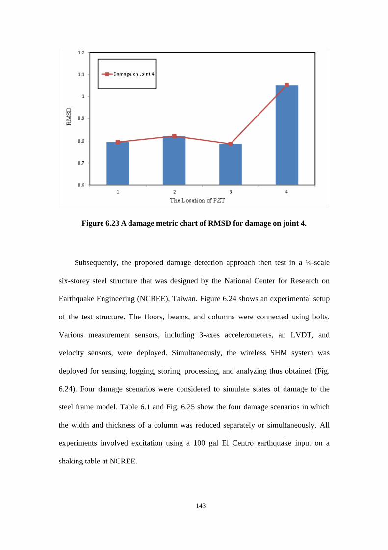
143

Figure 6.23 A damage metric chart of RMSD for damage on joint 4.

Subsequently, the proposed damage detection approach then test in a ¼ -scale

six-storey steel structure that was designed by the National Center for Research on

Earthquake Engineering (NCREE), Taiwan. Figure 6.24 shows an experimental setup

of the test structure. The floors, beams, and columns were connected using bolts.

Various measurement sensors, including 3-axes accelerometers, an LVDT, and

velocity sensors, were deployed. Simultaneously, the wireless SHM system was

deployed for sensing, logging, storing, processing, and analyzing thus obtained (Fig.

6.24). Four damage scenarios were considered to simulate states of damage to the

steel frame model. Table 6.1 and Fig. 6.25 show the four damage scenarios in which

the width and thickness of a column was reduced separately or simultaneously. All

experiments involved excitation using a 100 gal El Centro earthquake input on a

shaking table at NCREE.

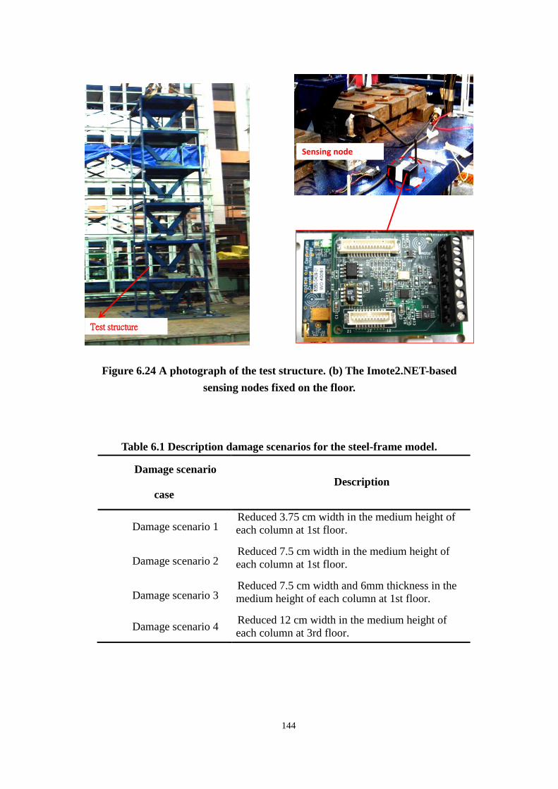
144

Figure 6.24 A photograph of the test structure. (b) The Imote2.NET-based

sensing nodes fixed on the floor.

Table 6.1 Description damage scenarios for the steel-frame model.

Damage scenario

case

Description

Damage scenario 1 Reduced 3.75 cm width in the medium height of

each column at 1st floor.

Damage scenario 2 Reduced 7.5 cm width in the medium height of

each column at 1st floor.

Damage scenario 3 Reduced 7.5 cm width and 6mm thickness in the

medium height of each column at 1st floor.

Damage scenario 4 Reduced 12 cm width in the medium height of

each column at 3rd floor.

Sensing node

Ttest

structure

Test structure

145

Figure 6.25 Photographer of damage scenario: (a) damage scenario 1. (b)

damage scenario 2. (c) damage scenario 3. (d) damage scenario 4.

The proposed WSN-based SHM system was deployed on a steel frame model.

The measurement period was 60s, during which data were sampled at 200 Hz.

Besides using the proposed reliable data-sensing and transmission service, a

time-scheduling data transmission procedure was used to transfer raw data to the base

station. The reliable data-sensing and transmission service provides excellent data

sensing and transmission quality for determining the structural dynamic properties.

Measured dynamic responses were acquired by wireless sensing nodes and reference

sensors. Figure 6.26 compares the acceleration time history measured by sensing

nodes and reference sensor. Using the steel frame responses, modal properties were

146

identified by the system identification procedure. In Table 6.2, the modal parameters

identified using the ANN-based system identification approach [139] were compared

with the measured data obtained by wireless sensing nodes and conventional

reference sensors. It is confirmed that the data obtained using the wireless sensing

nodes possess good quality and can be utilized reasonably to calculate the modal

parameters. Figure 6.27 (a)-(f) show the FRF of structure for 1st floor to 6

th floor.

147

Figure 6.26 Acceleration of wireless sensor and reference sensor

148

(a)

(b)

149

(c)

(d)

150

(e)

(f)

Figure 6.27. FRF of the structure: (a)1F, (b)2F, (c)3F, (d)4F, (e)5F, (d)6F

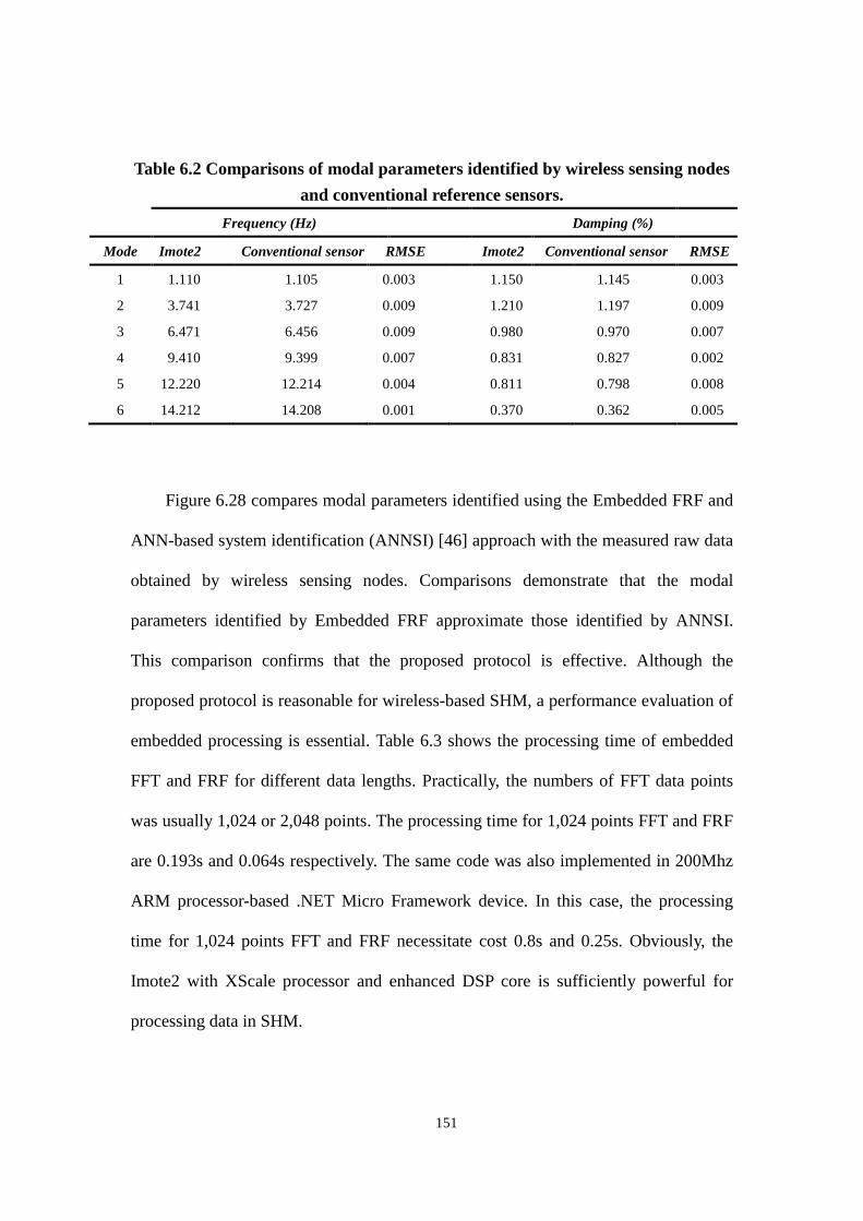
151

Table 6.2 Comparisons of modal parameters identified by wireless sensing nodes

and conventional reference sensors.

Frequency (Hz) Damping (%)

Mode Imote2 Conventional sensor RMSE Imote2 Conventional sensor RMSE

1 1.110 1.105 0.003 1.150 1.145 0.003

2 3.741 3.727 0.009 1.210 1.197 0.009

3 6.471 6.456 0.009 0.980 0.970 0.007

4 9.410 9.399 0.007 0.831 0.827 0.002

5 12.220 12.214 0.004 0.811 0.798 0.008

6 14.212 14.208 0.001 0.370 0.362 0.005

Figure 6.28 compares modal parameters identified using the Embedded FRF and

ANN-based system identification (ANNSI) [46] approach with the measured raw data

obtained by wireless sensing nodes. Comparisons demonstrate that the modal

parameters identified by Embedded FRF approximate those identified by ANNSI.

This comparison confirms that the proposed protocol is effective. Although the

proposed protocol is reasonable for wireless-based SHM, a performance evaluation of

embedded processing is essential. Table 6.3 shows the processing time of embedded

FFT and FRF for different data lengths. Practically, the numbers of FFT data points

was usually 1,024 or 2,048 points. The processing time for 1,024 points FFT and FRF

are 0.193s and 0.064s respectively. The same code was also implemented in 200Mhz

ARM processor-based .NET Micro Framework device. In this case, the processing

time for 1,024 points FFT and FRF necessitate cost 0.8s and 0.25s. Obviously, the

Imote2 with XScale processor and enhanced DSP core is sufficiently powerful for

processing data in SHM.

152

Figure 6.28 Comparisons of modal parameters identified by Embedded FRF and

ANNSI.

Table 6.3 The processing time of embedded FFT and FRF for different data

length.

Data length

512 1024 2048 4096

FFT 0.089s 0. 193s 0. 442s 0.970s

FRF 0.032s 0.064s 0.130s 0.259s

Total 0.121s 0.256s 0.572s 1.229s

Numerically simulated responses demonstrate that the proposed SubFRFDI can

be successfully used to identify the damage locations. The proposed SubFRFDI was

further applied to identifying damage locations in the experimental frame. Figure 6.29

shows the SubFRFDI for damage scenarios 1–4. The highest SubFRFDI value

indicates that the severest damage was located on the first floor in damage scenarios

1–3 (Figs. 6.29(a)– (c)). The SubFRFDI also indicates the damage location on the

third floor in damage scenario 4 (Fig. 6.29(d)).

153

154

Figure 6.29 The SubFRFDI for damage scenarios 1–4.

Subsequently, the EMI based damage detection approach then check the

component of building structure locally. Five PZT patches are respectively bonded to

the the columns in 1st floor as shown in Figure 6.30. The damage metric chart based

on RMSD is constructed to identify the local damage. As shown in Fig. 6.31-33, the

highest value locates the damage of location 5 significantly. As can be seen in the Fig

155

6.34, with an increase in extent of damage, there is a corresponding increase in the

damage metric values. Although the impedance method cannot exactly determine the

exact extent of the damage, an increasing damage metric with increased severity of

damage provides slightly quantitative information on the conditions of a structure.

Figure 6.30 PZT setup on the test structure.

1700 mm 1700 mm

1000 mm 1500 mm

6@

10

00

mm

X dir (North). Y dir (West).

Accelerometer

Displacement

Velocity

Strain Gage

S7 S6 S6 S9

Bolt1

Bolt2

Bolt3

Bolt4

PZT1 PZT2

PZT3 PZT4

PZT5

Crack

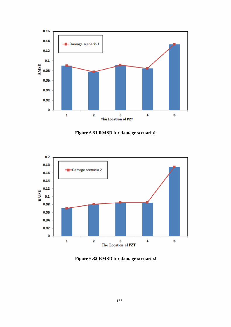
156

Figure 6.31 RMSD for damage scenario1


157


Figure 6.34 RMSD for three damage scenarios

158

CHAPHER 7 CONCLUSIONS REMARKS

7.1 Conclusion

A novel framework of an integrated wireless sensor network-based structural

health monitoring system in buildings and civil infrastructures was developed in this

study. The architecture of this SHM system was presented. A global-local-integrated

damage detection approach was also developed for damage detection. Numerical and

experimental studies were conducted to verify the applicability of the proposed

approach. The following conclusions are drawn based on the integrated WSN-based

SHM system, global-local-integrated damage detection approach and experimental

results.

Integrated WSN-based SHM system

The Integrated WSN-based SHM system was developed in this study. This

system architecture consists of sensing nodes, cluster head nodes, transfer node, and

base station. Each sensing node is based on Imote2 platform which is comprised of a

microprocessor, sensor module, and communication device. The cluster head is a dule

core design which combine Imote2 platform and second embedded device. The

cluster head has extra wireless module and GPS. The base station is the highest level

end device that has largest memory, most powerful processor and highest

communication capability.

A new sensor board was developed. This sensor board integrates a six degrees of

freedom inertial measurement unit (6 DoF IMU) SD746 sensor chip and a GPS

module. In this system, a novel windmill-magnet integrated piezoelectric (WMIP)

159

energy harvesting system was also developed.

The proposed software system of integrated WSN-based SHM system is a

three-tier-framework, i.e., node, logging and processing tiers. The application

functions are developed in a Microsoft NETMF environment. The NETMF and

Crossbow’s API, i.e., application interface provided by manufacturing company of

Imote2, assist most libraries in dealing with all peripherals and drivers, allowing us to

develop individual applications for the SHM efficiently. The proposed user interface

shows how the sensor data can be represented in a Fig. chart and nodes distribution

can also be conveniently observed.

WSN-based middleware services for SHM application are developed. The

middleware services include reliable data-sensing and transmission, which are data

aggregation, reliable communication, and synchronized sensing. These middleware

services are implemented on the nodes running .NETMF and are generally applicable

to SHM application.

Global-local-integrated damage detection approach

This study developed a global-local-integrated damage detection approach. In the

first stage, the global approach detected changes in characteristics of the overall. After

identifying the damage and its approximate location, the second stage used local

detection method to identify the detailed conditions of the damage.

Substructure-based frequency response function and wavelet energy distribution

approaches are proposed for use in global damage detection. Local structural damage

is detected using an EMI-based method. Numerical results confirm the effectiveness

of the global-local-integrated damage detection approach for locating damage.

160

Experimental results

In experimental study, First off all, the integrated WSN-based SHM system is

verified involving sensor calibration, wireless communication quality, data losing,

interference in material, power consumption. The verification of sensing node

indicates the good-quality data collection by the wireless sensing system and the

modal parameters of structure can be correctly calculated by this system. In reliability

of RF communication test indicates that the proposed system is robust and stable for

long term monitoring via the proposed reliable data-sensing and transmission service.

This system was deployed in Nioudou Bridge. A field free vibration test was

conducted for obtaining dynamic response. The good-quality data collection by the

wireless sensing system successfully records a typical free vibration response of the

pier. By comparing two FFTs for intact and scouring case, in frequency domain, the

difference between intact and scouring case can be observed. The work indicates that

the proposed wireless sensing system was a reliable technology for monitoring Bridge

structure.

The proposed damage detection approach then was tested in a ¼ -scale six-storey

steel structure. Experimental analysis using global SHM approach shows that, both

SubFRFDI can indicates the approximate location of the damaged area, then the

EMI-based damage detection approach can check the components of the building

structure locally. The damage metric chart based on RMSD is constructed to identify

the position of local damage to the structure.

161

7.2 Future Study

Following the unfinished works and the drawbacks of the proposed approaches,

some potential directions on the future research are brought out.

In the proposed system, the main sensor on the sensing node is an accelerometer.

However, the resolution of this accelerometer can works well on detection large

vibration such as structural response excited by earthquake. For ambient vibration,

new sensor board should be developed in the future work.

This study proposed a novel windmill-magnet integrated piezoelectric (WMIP)

energy harvesting system. In the future work, the multiple energy harvesting methods

such as solar, piezoelectric and wind should be integrated. The energy harvesting

circuit needs to be included in the mote. Moreover, wireless power technology could

be considered a feasible plan for WSN in SHM.

This works developed a structure of class libraries which is branch out into three

basic class of NETMF, basic class library of Imote2, and SHM class. The SHM class,

a specialized class, is developed by this study for SHM application. However, in this

SHM class only FFT and FRF were included. In the future work, more embedded

signal processing class like wavelet should be developed.

Substructure-based frequency response function approaches are proposed for use

in global damage detection. However, these methods only focus on detecting and

locating damage. Further study should be conducted in deciding the extent of damage

in structure. EMI-based method was used to detect the local damage herein. In the

future work, the EMI-based sensor node should be developed and the local damage

index should be embedded in the node.

162

In experimental study, the developed integrated WSN-based SHM system was

deployed in a steel structure and in a bridge. The experimental result indicates this

system performs well either in Lab or in field test. In the future work, this system will

be considered deploying in different civil structure. When deploying in a large scaled

structure, the software and hardware of the system should be improved and modified.

An optimization approach can also be applied for deploying great amount sensor

nodes in the future works.

163

REFERENCE

1. Adams, D.E., Health monitoring of structural materials and components.

Methods with Applications. Willey, New York, 2007.

2. Worden, K., Farrar, C.R., Haywood, J., and Todd, M., A review of nonlinear

dynamics applications to structural health monitoring. Structural Controal and

Mealth Monitoring, 2008. 15(4): p. 540-567.

3. Sohn, H., Farrar, C.R., Hemez, F.M., Shunk, D.D., Stinemates, D.W., and

Nadler, B.R., A review of structural health monitoring literature: 1996-2001.

2004, Los Alamos National Laboratory.

4. Doebling, S.W., Farrar, C.R., and Prime, M.B., A summary review of

vibration-based damage identification methods. Shock and Vibration Digest,

1998. 30(2): p. 91-105.

5. Sohn, H. and Laboratory, L.A.N., A review of structural health monitoring

literature: 1996-2001. 2004: Los Alamos National Laboratory.

6. Inman, D.J., Damage prognosis for aerospace, civil and mechanical systems.

2005: John Wiley & Sons Inc.

7. Ansari, F., Sensing issues in civil structural health monitoring. 2005: Kluwer

Academic Pub.

8. Chang, P., Flatau, A., and Liu, S., Review paper: health monitoring of civil

infrastructure. Structural Health Monitoring, 2003. 2(3): p. 257.

9. Farrar, C., Historical overview of structural health monitoring, in Lecture notes

on structural health monitoring using statistical pattern recognition. 2001, Los

Alamos Dynamics, Los Alamos, NM.

10. Celebi, M., Seismic instrumentation of buildings (with emphasis on federal

buildings), in Special GSA/USGS Project, an administrative report. 2002,

United States Geological Survey: Menlo Park, CA.

11. Nagayama, T., Sim, S., Miyamori, Y., and Spencer Jr, B., Issues in structural

health monitoring employing smart sensors. Smart Structures and Systems,

2007. 3(3): p. 299-320.

12. Lynch, J.P. and Loh, K.J., A summary review of wireless sensors and sensor

networks for structural health monitoring. Shock and Vibration Digest, 2006.

164

38(2): p. 91-130.

13. Spencer Jr, B.F., Ruiz-Sandoval, M.E., and Kurata, N., Smart sensing

technology: opportunities and challenges. Structural Control & Health

Monitoring, 2004. 11(4): p. 349-368.

14. Chavali, M., Lin, T.H., Wu, R.J., Luk, H.N., and Hung, S.L., Active 433

MHz-W UHF RF-powered chip integrated with a nanocomposite

m-MWCNT/polypyrrole sensor for wireless monitoring of volatile anesthetic

agent sevoflurane. Sensors and Actuators a-Physical, 2008. 141(1): p. 109-119.

15. Xu, N., Rangwala, S., Chintalapudi, K., Ganesan, D., Broad, A., Govindan, R.,

and Estrin, D. A wireless sensor network for structural monitoring. Proceeding

of 2nd international conference on Embedded networked sensor systems.

2004.

16. Yuan, S.F., Lai, X.S., Zhao, X., Xu, X., and Zhang, L., Distributed structural

health monitoring system based on smart wireless sensor and multi-agent

technology. Smart Materials & Structures, 2006. 15(1): p. 1-8.

17. Kurata, N., Spencer Jr, B., Ruiz-Sandoval, M., Miyamoto, Y., and Sako, Y., A

study on building risk monitoring using wireless sensor network MICA mote.

Strain, 2003. 1: p. 35.

18. Kim, S., Pakzad, S., Culler, D., Demmel, J., Fenves, G., Glaser, S., and Turon,

M. Health monitoring of civil infrastructures using wireless sensor networks.

Proceeding of 6th international conference on Information processing in

sensor networks. 2007.

19. Doebling, S.W., Farrar, C.R., and Goodman, R.S. Effects of measurement

statistics on the detection of damage in the Alamosa Canyon Bridge. Proceeding

of Proceedings 15th International Modal Analysis Conference. 1997.

20. Farrar, C.R., Doebling, S.W., Cornwell, P.J., and Straser, E.G. Variability of

modal parameters measured on the Alamosa Canyon Bridge. Proceeding of

Proceedings 15th International Modal Analysis Conference. 1997.

21. Doebling, S.W., Farrar, C.R., Prime, M.B., and Shevitz, D.W., Damage

identification and health monitoring of structural and mechanical systems from

changes in their vibration characteristics: a literature review. 1996, Los Alamos

National Lab., NM (United States).

22. Salawu, O., Detection of structural damage through changes in frequency: a

165

review. Engineering Structures, 1997. 19(9): p. 718-723.

23. West, W.M. Illustration of the use of modal assurance criterion to detect

structural changes in an orbiter test specimen. Proceeding of Air Force

Conference on Aircraft Structural Integrity. 1986.

24. Mayes, R., Error localization using mode shapes: An application to a two link

robot arm, in 10th International Modal Analysis Conference. 1991, Sandia

National Labs., Albuquerque, NM (United States): Albuquerque, NM.

25. Kam, T. and Lee, T., Detection of cracks in structures using modal test data.

Engineering fracture mechanics, 1992. 42(2): p. 381-387.

26. Ko, J., Wong, C., and Lam, H. Damage detection in steel framed structures by

vibration measurement approach. Proceeding of 12th International Modal

Analysis Conference. 1994.

27. Farrar, C.R. and Doebling, S.W. An overview of modal-based damage

identification methods. Proceeding of DAMAS Conference. 1997.

28. Fox, C. The location of defects in structures-A comparison of the use of natural

frequency and mode shape data. Proceeding of the 10th International Modal

Analysis Conference. 1992.

29. Pandey, A., Biswas, M., and Samman, M., Damage detection from changes in

curvature mode shapes. Journal of Sound and Vibration, 1991. 145(2): p.

321-332.

30. Topole, K.G. and Stubbs, N., Non destructive damage evaluation of a structure

from limited modal parameters. Earthquake Engineering & Structural

Dynamics, 1995. 24(11): p. 1427-1436.

31. Chance, J., Tomlinson, G., and Worden, K. A simplified approach to the

numerical and experimental modelling of the dynamics of a cracked beam.

Proceedings of the 12th International Modal Analysis Conference. 1994.

32. Chen, J.C. and Garbat, J.A., Analytical model improvement using modal test

results. Aiaa Journal, 1980. 18: p. 684-690.

33. SMITH, S. Iterative use of direct matrix updates- Connectivity and convergence.

Proceeding of 33rd AIAA Structures, Structural Dynamics and Materials

Conference. 1992.

34. Liu, P.L., Identification and damage detection of trusses using modal data.

166

Journal of Structural Engineering, 1995. 121(4): p. 599-608.

35. KAOUK, M. and Zimmerman, D.C., Structural damage assessment using a

generalized minimum rank perturbation theory. Aiaa Journal, 1994. 32(4): p.

836-842.

36. Hemez, F. and Farhat, C., Structural damage detection via a finite element

model updating methodology. MODAL ANALYSIS-The International Journal

of Analytical and Experimental Modal Analysis, 1995. 10(3): p. 152-166.

37. Norris, M.A. and Meirovitch, L., On the problem of modelling for parameter

identification in distributed structures. International Journal for Numerical

Methods in Engineering, 1989. 28(10): p. 2451-2463.

38. Haug, E. and Choi, K., Structural design sensitivity analysis with generalized

global stiffness and mass matrices. Aiaa Journal, 1984. 22(9): p. 1299-1303.

39. Ricles, J. and Kosmatka, J., Damage detection in elastic structures using

vibratory residual forces and weighted sensitivity. Aiaa Journal, 1992. 30(9): p.

2310-2316.

40. Lim, T.W. and Kashangaki, T.A.L., Structural damage detection of space truss

structures using best achievable eigenvectors. Aiaa Journal, 1994. 32: p.

1049-1057.

41. Zimmerman, D.C. and MOHAMED, K., Eigenstructure assignment approach

for structural damage detection. Aiaa Journal, 1992. 30(7): p. 1848-1855.

42. Sohn, H., Farrar, C.R., Hunter, N.F., and Worden, K., Structural Health

Monitoring Using Statistical Pattern Recognition Techniques. Journal of

Dynamic Systems, Measurement, and Control, 2001. 123(4): p. 706-711.

43. Lei, Y., Kiremidjian, A., Nair, K., Lynch, J., Law, K., Kenny, T., Carryer, E.,

and Kottapalli, A. Statistical damage detection using time series analysis on a

structural health monitoring benchmark problem. Proceeding of 9th

International Conference on Applications of Statistics and Probability in Civil

Engineering. 2003.

44. Chen, H., Qi, G., Yang, J., and Amini, F., Neural network for structural

dynamic model identification. Journal of engineering mechanics, 1995. 121: p.

1377.

45. Wu, X., Ghaboussi, J., and Garrett, J., Use of neural networks in detection of

structural damage. Computers & Structures, 1992. 42(4): p. 649-659.

167

46. Wen, C.M., Hung, S.L., Huang, C.S., and Jan, J.C., Unsupervised fuzzy neural

networks for damage detection of structures. Structural Controal and Mealth

Monitoring, 2007. 14(1): p. 144-161.

47. Kudva, J., Munir, N., and Tan, P., Damage detection in smart structures using

neural networks and finite-element analyses. Smart Materials and Structures,

1992. 1: p. 108.

48. Poudel, U., Fu, G., and Ye, J., Structural damage detection using digital video

imaging technique and wavelet transformation. Journal of Sound and

Vibration, 2005. 286(4-5): p. 869-895.

49. Kim, H. and Melhem, H., Damage detection of structures by wavelet analysis.

Engineering Structures, 2004. 26(3): p. 347-362.

50. Ovanesova, A.V. and Suárez, L.E., Applications of wavelet transforms to

damage detection in frame structures. Engineering Structures, 2004. 26(1): p.

39-49.

51. Huang, C.S. and Su, W.C., Identification of modal parameters of a time

invariant linear system by continuous wavelet transformation. Mechanical

Systems and Signal Processing, 2007. 21(4): p. 1642-1664.

52. Huang, C.S., Hung, S.L., Lin, C.I., and Su, W.C., A wavelet-based approach to

identifying structural modal parameters from seismic response and free

vibration data. Computer-Aided Civil and Infrastructure Engineering, 2005.

20(6): p. 408-423.

53. Wu, N. and Wang, Q., Experimental studies on damage detection of beam

structures with wavelet transform. International Journal of Engineering

Science, 2011. 49(3): p. 253-261.

54. Han, J.-G., Ren, W.-X., and Sun, Z.-S., Wavelet packet based damage

identification of beam structures. International Journal of Solids and

Structures, 2005. 42(26): p. 6610-6627.

55. Poornachandra, S., Wavelet-based denoising using subband dependent

threshold for ECG signals. Digital Signal Processing, 2008. 18(1): p. 49-55.

56. Pasti, L., Walczak, B., Massart, D.L., and Reschiglian, P., Optimization of

signal denoising in discrete wavelet transform. Chemometrics and Intelligent

Laboratory Systems, 1999. 48(1): p. 21-34.

57. Lee, B. and Tarng, Y., Drill fracture detection by the discrete wavelet transform.

168

Journal of Materials Processing Technology, 2000. 99(1-3): p. 250-254.

58. Prabhakar, S., Mohanty, A., and Sekhar, A., Application of discrete wavelet

transform for detection of ball bearing race faults. Tribology International,

2002. 35(12): p. 793-800.

59. Sansalone, M., Carino, N.J., and Division, C.f.B.T.S., Impact-echo: a method

for flaw detection in concrete using transient stress waves. 1986: US Dept. of

Commerce, National Bureau of Standards, Center for Building Technology,

Structures Division.

60. Davis, A.G., Evans, J.G., and Hertlein, B.H., Nondestructive evaluation of

concrete radioactive waste tanks. Journal of performance of constructed

facilities, 1997. 11: p. 161.

61. Chady, T., Enokizono, M., and Sikora, R., Crack detection and recognition

using an eddy current differential probe. Magnetics, IEEE Transactions on,

1999. 35(3): p. 1849-1852.

62. Tian, G.Y., Sophian, A., Taylor, D., and Rudlin, J., Multiple sensors on pulsed

eddy-current detection for 3-D subsurface crack assessment. Sensors Journal,

IEEE, 2005. 5(1): p. 90-96.

63. Washer, G.A. Detection of fatigue cracks in eyebars using time of flight

diffraction. Proceeding of Conf. on StructuralMaterials Technology and

Nondestructive Testing. 1996.

64. Liang, C., Sun, F., and Rogers, C., Coupled Electro-Mechanical Analysis of

Adaptive Material Systems--Determination of the Actuator Power Consumption

and System Energy Transfer. Journal of Intelligent Material Systems and

Structures, 1994. 5(1): p. 12.

65. Sun, F., Rogers, C.A., and Liang, C. Structural frequency response function

acquisition via electric impedance measurement of surface-bonded piezoelectric

sensor/actuator. Proceeding of Structures, Structural Dynamics, and

Materials Conference. 1995.

66. Chaudhry, Z., Lalande, F., Ganino, A., and Rogers, C. Monitoring the integrity

of composite patch structural repair via piezoelectric actuators/sensors.

Proceeding of 36th AIAA/ASME/ASCE/AHS/ASC Structures, Structural

Dynamics, and Materials Conference. 1995.

67. Park, G., Kabeya, K., Cudney, H.H., and Inman, D.J., Impedance-based

169

structural health monitoring for temperature varying applications. JSME

international journal. Series A, Solid mechanics and material engineering,

1999. 42(2): p. 249-258.

68. Park, G., Cudney, H.H., and Inman, D.J., Impedance-based health monitoring

of civil structural components. Journal of Infrastructure Systems, 2000. 6(4): p.

153-160.

69. Yang, Y., Hu, Y., and Lu, Y., Sensitivity of PZT impedance sensors for damage

detection of concrete structures. Sensors, 2008. 8(1): p. 327-346.

70. Kim, J., Vibration and impedance monitoring for prestress-loss prediction in

PSC girder bridges. Smart Structures and Systems, 2009. 5(1): p. 81-94.

71. Park, G., Sohn, H., Farrar, C.R., and Inman, D.J., Overview of piezoelectric

impedance-based health monitoring and path forward. Shock and Vibration

Digest, 2003. 35(6): p. 451-464.

72. Mascarenas, D., Flynn, E., Todd, M., Park, G., and Farrar, C., Wireless Sensor

Technologies for Monitoring Civil Structures. Sound and Vibration, 2008. 42(4):

p. 16.

73. Kim, S., Pakzad, S., Culler, D., Demmel, J., Fenves, G., Glaser, S., and Turon,

M. Health monitoring of civil infrastructures using wireless sensor networks.

Proceeding of 6th international conference on Information processing in

sensor networks 2007.

74. Cho, S., Jang, S.A., Jo, H., Mechitov, K., Rice, J.A., Jung, H.J., Yun, C.B.,

Spencer Jr, B.F., Nagayama, T., and Seo, J. Structural health monitoring

system of a cable-stayed bridge using a dense array of scalable smart sensor

network. Proceeding of Sensors and Smart Structures Technologies for Civil,

Mechanical, and Aerospace Systems. 2010.

75. Hoult, N.A., Fidler, P.R.A., Hill, P.G., and Middleton, C.R., Long-term wireless

structural health monitoring of the Ferriby Road Bridge. Journal of Bridge

Engineering, 2010. 15: p. 153.

76. Kim, J., Lynch, J.P., Lee, J.J., and Lee, C.G., Truck-based mobile wireless

sensor networks for the experimental observation of vehicle¡Vbridge interaction.

Smart Materials and Structures, 2011. 20: p. 065009.

77. Castillo-Effer, M., Quintela, D.H., Moreno, W., Jordan, R., and Westhoff, W.

Wireless sensor networks for flash-flood alerting. Proceeding of the Fifth IEEE

170

International Caracas Conference on Devices. 2004.

78. Simon, G., Maroti, M., Ledeczi, A., Balogh, G., Kusy, B., Nadas, A., Pap, G.,

Sallai, J., and Frampton, K. Sensor network-based countersniper system.

Proceeding of the 2nd international conference on Embedded networked

sensor systems 2004.

79. Werner-Allen, G., Lorincz, K., Welsh, M., Marcillo, O., Johnson, J., Ruiz, M.,

and Lees, J., Deploying a wireless sensor network on an active volcano. Ieee

Internet Computing, 2006: p. 18-25.

80. Akyildiz, I.F., Su, W., Sankarasubramaniam, Y., and Cayirci, E., Wireless

sensor networks: a survey. Computer Networks-the International Journal of

Computer and Telecommunications Networking, 2002. 38(4): p. 393-422.

81. Yick, J., Mukherjee, B., and Ghosal, D., Wireless sensor network survey.

Computer Networks, 2008. 52(12): p. 2292-2330.

82. Younis, M. and Akkaya, K., Strategies and techniques for node placement in

wireless sensor networks: A survey. Ad Hoc Networks, 2008. 6(4): p. 621-655.

83. Nagayama, T., Spencer Jr, B.F., Mechitov, K.A., and Agha, G.A., Middleware

services for structural health monitoring using smart sensors. Smart Structures

and Systems, 2009. 5(2): p. 119-137.

84. Lynch, J.P., An overview of wireless structural health monitoring for civil

structures. Philosophical Transactions of the Royal Society a-Mathematical

Physical and Engineering Sciences, 2007. 365(1851): p. 345-372.

85. Cho, S., Yun, C.B., Lynch, J.P., Zimmerman, A.T., Spencer, B.F., and

Nagayama, T., Smart Wireless Sensor Technology for Structural Health

Monitoring of Civil Structures. International Journal of Steel Structures, 2008.

8(4): p. 267-275.

86. Paek, J., Chintalapudi, K., Govindan, R., Caffrey, J., and Masri, S. A wireless

sensor network for structural health monitoring: Performance and experience.

Proceeding of The Second IEEE Workshop on Embedded Networked Sensors

(EmNetS-II). 2005.

87. Straser, E.G., Kiremidjian, A.S., and Center, J.A.B.E.E., A modular, wireless

damage monitoring system for structures. 1998: The John A. Blume

Earthquake Engineering Center.

88. Lynch, J.P., Law, K.H., Kiremidjian, A.S., Kenny, T.W., Carryer, E., and

171

Partridge, A. The design of a wireless sensing unit for structural health

monitoring. Proceeding of 3rd Int’l Ws. Structural Health Monitoring. 2001.

89. Wang, Y., Lynch, J.P., and Law, K.H., Validation of an integrated network

system for real-time wireless monitoring of civil structures. Structural health

monitoring, 2005: advancements and challenges for implementation, 2005.

1050(48109): p. 275.

90. Aoki, S., Fujino, Y., and Abe, M. Intelligent bridge maintenance system using

MEMS and network technology. Proceeding of SPIE Conf. 2003.

91. Chung, H.C., Enomoto, T., Shinozuka, M., Chou, P., Park, C., Yokoi, I., and

Morishita, S. Real-time visualization of structural response with wireless

MEMS sensors. Proceeding of 13th world conf. Earthquake Engineering.

2004.

92. Farrar, C.R., Allen, D.W., Park, G., Ball, S., and Masquelier, M.P., Coupling

sensing hardware with data interrogation software for structural health

monitoring. Shock and Vibration, 2006. 13(4): p. 519-530.

93. Chen, B. and Liu, W., Mobile agent computing paradigm for building a flexible

structural health monitoring sensor network. Computer Aided Civil and

Infrastructure Engineering, 2010. 25(7): p. 504-516.

94. Xu, N., Rangwala, S., Chintalapudi, K.K., Ganesan, D., Broad, A., Govindan,

R., and Estrin, D., A wireless sensor network For structural monitoring.

Proceedings of the 2nd international conference on Embedded networked

sensor systems, 2004: p. 13-24.

95. ShenfangYuan, X.L., Zhao, X., Xu, X., and Zhang, L., Distributed structural

health monitoring system based on smart wireless sensor and multi-agent

technology. Smart Mater. Struct, 2006. 15: p. 1-8.

96. Kurata, N., Spencer Jr, B.F., Ruiz-Sandoval, M., Miyamoto, Y., and Sako, Y.,

A study on building risk monitoring using wireless sensor network MICA mote.

Strain. 1: p. 35.

97. Hoblos, G., Staroswiecki, M., and Aitouche, A. Optimal design of fault tolerant

sensor networks. Proceeding of IEEE International Conference on Control

Applications. 2000.

98. Cho, S.H. and Chandrakasan, A.P. Energy efficient protocols for low duty cycle

wireless microsensor networks. Proceeding of 33rd Annual Hawaii

172

International Conference on System Sciences. 2001.

99. Rabaey, J.M., Ammer, M.J., da Silva Jr, J.L., Patel, D., and Roundy, S.,

PicoRadio supports ad hoc ultra-low power wireless networking. Computer,

2000. 33(7): p. 42-48.

100. Intanagonwiwat, C., Govindan, R., and Estrin, D. Directed diffusion: A

scalable and robust communication paradigm for sensor networks. Proceeding

of ACM Mobi-Com'00. 2000.

101. Kahn, J.M., Katz, R.H., and Pister, K.S.J. Next century challenges: mobile

networking for smart dust. Proceeding of ACM MobiCom’99. 1999.

102. Alliance, Z.B., ZigBee Specifications Version 1.0., San Ramon, CA, USA,

December. 2004. 2004.

103. Gutierrez, J.A., Naeve, M., Callaway, E., Bourgeois, M., Mitter, V., and Heile,

B., IEEE 802.15. 4: a developing standard for low-power low-cost wireless

personal area networks. Network, IEEE, 2001. 15(5): p. 12-19.

104. Woo, A., Madden, S., and Govindan, R., Networking support for query

processing in sensor networks. Communications of the Acm, 2004. 47(6): p.

47-52.

105. Kopetz, H., Damm, A., Koza, C., Mulazzani, M., Schwabl, W., Senft, C., and

Zainlinger, R., Distributed fault-tolerant real-time systems: The Mars approach.

Micro, IEEE, 1989. 9(1): p. 25-40.

106.Horauer, M., Schossmaier, K., Schmid, U., Holler, R., Kero, N., and ., V.U.O.T.

PSynUTC-Evaluation of a High-Precision Time Synchronization Prototype

System for Ethernet LANs. Proceeding of 34th Annual Precise Time and Time

Interval Meeting (PTTI). 2002.

107. Mills, D.L., Internet time synchronization: The network time protocol.

Communications, IEEE Transactions on, 1991. 39(10): p. 1482-1493.

108. Syed, A. and Heidemann, J. Time synchronization for high latency acoustic

networks. Proceeding of IEEE Infocom. 2006.

109. Nagayama, T., Spencer, B.F., and Rice, J.A., Autonomous decentralized

structural health monitoring using smart sensors. Structural Control & Health

Monitoring, 2009. 16(7-8): p. 842-859.

110. Lanzara, G., Feng, J., and Chang, F.K., Design of micro-scale highly

173

expandable networks of polymer-based substrates for macro-scale applications.

Smart Materials & Structures, 2010. 19(4): p. 045013.

111. Gratzel, M., Solar energy conversion by dye-sensitized photovoltaic cells. Inorg.

Chem, 2005. 44(20): p. 6841-6851.

112. Sodano, H., Simmers, G., Dereux, R., and Inman, D., Recharging batteries

using energy harvested from thermal gradients. Journal of Intelligent Material

Systems and Structures, 2007. 18(1): p. 3.

113. Beeby, S., Tudor, M., and White, N., Energy harvesting vibration sources for

microsystems applications. Measurement Science and Technology, 2006. 17: p.

R175.

114. Ottman, G., Hofmann, H., Bhatt, A., and Lesieutre, G., Adaptive piezoelectric

energy harvesting circuit for wireless remote power supply. IEEE Transactions

on Power Electronics, 2002. 17(5): p. 669-676.

115. Ganeriwal, S., Kumar, R., and Srivastava, M. Timing-sync protocol for sensor

networks. Proceeding of 1st international conference on Embedded networked

sensor systems. 2003.

116. Cauberghe, B., Guillaume, P., Verboven, P., Vanlanduit, S., and Parloo, E.,

Frequency response function-based parameter identification from short data

sequences. Mechanical Systems and Signal Processing, 2004. 18(5): p.

1097-1116.

117. Celic, D. and Boltezar, M., Identification of the dynamic properties of joints

using frequency-response functions. Journal of Sound and Vibration, 2008.

317(1-2): p. 158-174.

118. Wang, Z., Lin, R.M., and Lim, M.K., Structural damage detection using

measured FRF data. Computer Methods in Applied Mechanics and

Engineering, 1997. 147(1-2): p. 187-197.

119. Lee, U. and Shin, J., A frequency-domain method of structural damage

identification formulated from the dynamic stiffness equation of motion.

Journal of Sound and Vibration, 2002. 257(4): p. 615-634.

120. Thyagarajan, S.K., Schulz, M.J., Pai, P.F., and Chung, J., Detecting structural

damage using frequency response functions. Journal of Sound and Vibration,

1998. 210(1): p. 162-170.

121. Lee, U. and Shin, J., A frequency response function-based structural damage

174

identification method. Computers and Structures, 2002. 80(2): p. 117-132.

122. Sampaio, R.P.C., Maia, N.M.M., and Silva, J.M.M., Damage detection using

the frequency-response-function curvature method. Journal of Sound and

Vibration, 1999. 226(5): p. 1029-1042.

123. Maia, N.M.M., Silva, J.M.M., Almas, E.A.M., and Sampaio, R.P.C., Damage

detection in structures: from mode shape to frequency response function

methods. Mechanical Systems and Signal Processing, 2003. 17(3): p. 489-498.

124. Liu, X., Lieven, N.A.J., and Escamilla-Ambrosio, P.J., Frequency response

function shape-based methods for structural damage localisation. Mechanical

Systems and Signal Processing, 2009. 23(4): p. 1243-1259.

125. Ni, Y.Q., Zhou, X.T., and Ko, J.M., Experimental investigation of seismic

damage identification using PCA-compressed frequency response functions and

neural networks. Journal of Sound and Vibration, 2006. 290(1-2): p. 242-263.

126. Furukawa, A., Otsuka, H., and Kiyono, J., Structural damage detection

method using uncertain frequency response functions. Computer-Aided Civil

and Infrastructure Engineering, 2006. 21(4): p. 292-305.

127. Kanwar, V.S., Kwatra, N., Aggarwal, P., and Gambir, M.L., Health

monitoring of RCC building model experimentally and its analytical validation.

Engineering Computations, 2008. 25(7-8): p. 677-693.

128. Hsu, T. and Loh, C. Damage detection using frequency response functions

under ground excitation. Proceeding of Sensors and Smart Structures

Technologies for Civil, Mechanical, and Aerospace Systems. 2009.

129. Park, G. and Inman, D., Structural health monitoring using piezoelectric

impedance measurements. Philosophical Transactions of the Royal Society A:

Mathematical, Physical and Engineering Sciences, 2007. 365(1851): p. 373.

130. Liang, C., Sun, F., and Rogers, C., Coupled electro-mechanical analysis of

adaptive material systems¡Xdetermination of the actuator power consumption

and system energy transfer. Journal of Intelligent Material Systems and

Structures, 1994. 5(1): p. 12.

131. Sun, F., Chaudhry, Z., Liang, C., and Rogers, C., Truss structure integrity

identification using PZT sensor-actuator. Journal of Intelligent Material

Systems and Structures, 1995. 6(1): p. 134-139.

132. Peairs, D.M., Park, G., and Inman, D.J., Improving accessibility of the

175

impedance-based structural health monitoring method. Journal of Intelligent

Material Systems and Structures, 2004. 15(2): p. 129.

133. Nokes, J. and Cloud, G., The application of interferometric techniques to the

nondestructive inspection of fiber-reinforced materials. Experimental

Mechanics, 1993. 33(4): p. 314-319.

134. Esteban, J., Modeling of the sensing region of a piezoelectric actuator/sensor.

1996, Ph. D. Dissertation, Virginia Polytechnic Institute and State University,

Blacksburg, VA.

135. Forde, M., McCann, D., Clark, M., Broughton, K., Fenning, P., and Brown,

A., Radar measurement of bridge scour. Ndt & E International, 1999. 32(8): p.

481-492.

136. Yankielun, N. and Zabilansky, L., Laboratory investigation of time-domain

reflectometry system for monitoring bridge scour. Journal of Hydraulic

engineering, 1999. 125(12): p. 1279-1284.

137. Lin, Y., Chen, J., Chang, K., Chern, J., and Lai, J., Real-time monitoring of

local scour by using fiber Bragg grating sensors. Smart Materials and

Structures, 2005. 14: p. 664.

138. DeVault, J., Robotic system for underwater inspection of bridge piers.

Instrumentation & Measurement Magazine, IEEE, 2002. 3(3): p. 32-37.

139. Huang, C.S., Hung, S.L., Wen, C.M., and Tu, T.T., A neural network approach

for structural identification and diagnosis of a building from seismic response

data. Earthquake Engineering & Structural Dynamics, 2003. 32(2): p.

187-206.

176

Vita

林子軒 (Tzu-Hsuan Lin)

個人資料

生日：1978/06/05

性別：男性

住址：新竹市東大路二段172巷1弄7號1樓

電話：03-5712121#54965, 0963354403

Email: [email protected]

兵役：役畢

現職

國立交通大學土木工程系博士候選人(指導教授:洪士林教授)

國立交通大學電機與控制工程研究所碩士班(指導教授:廖德誠教授)

學歷

2009.7~2009.9 東京大學訪問學生(Host: Professor Yozo Fujino )

2005.9 ~Now 國立交通大學土木工程研究所博士班結構組

2007.6~ Now 雙主修國立交通大學電機與控制工程研究所碩士班

2001.9 ~ 2003.6 國立交通大學土木工程研究所碩士

2001.9 ~ 2003.6 國立交通大學資訊管理研究所輔所

1997.9 ~ 2001.6 國立台北科技大學土木系(第一名畢業)

榮譽

2009.7~9 日本交流協會暑期交換學生獎學金(兩個月共，72 萬日幣)赴

東京大學研究，並獲選為得獎代表，上台致謝。(全國 18 名，

唯一的土木領域)

2010 中華顧問工程司，工程科技獎學金，博士班獎學金 10 萬元。

2007~2009 中興工程研究發展基金會博士班獎助學金 (土木領域全國最

高獎學金，每年 30 萬元)，連續三年獲獎

2006 中興工程顧問社優秀學生獎

mailto:[email protected]

177

研究成果目錄：論文及著述

A. 學位論文

林子軒，‖土木工程結構修復補強知識管理與支援決策輔助系統之研究” 碩士論

文，國立交通大學土木工程系，2003。

B. 期刊論文

[1] T. H. Lin, S. L. Hung, Y. C. Lu, T. Nagayama and Y. Fujino (2011),

Development of An Embedded Damage Detection Approach Using

Imote2.net-Based Wireless Structural Health Monitoring, Structural health

monitoring-an international journal. (Reviewing)

[2] T. H. Lin, S. L. Hung, C. S. Huang, and T. K. Lin (2012), Detection of damage

location using a novel substructure-based frequency response function approach

with a wireless sensing system, International Journal of Structural Stability and

Dynamics, has been accepted for publication in Vol. 12, No. 3 (June 2012)

IF:0.721

[3] T. H. Lin, S. L. Hung, M. Chavali, R. J. Wu, H. N. Luk and Q. Fei (2010),

Towards Development of Wireless Sensor System For Monitoring Anesthetic

Agents, Sensor Letters. 8, 767-776. IF:0.626

[4] R. J. Wu, Y. C. Huang, M. R. Yu, T. H. Lin, S. L. Hung (2008), Application of

m-CNTs/NaClO4/Ppy to A Fast Response, Room Working Temperature Ethanol

Sensor‖. Sensors and Actuators B: Chemical, 134(1), 213-218. IF:3.083

[5] Murthy Chavali , T. H. Lin, R.J. Wu, H.N. Luk and S.L. Hung (2008), ―Active

433 MHz-W UHF RF powered chip integrated with a nano composite

m-MWCNT/Polypyrrole sensor for wireless monitoring of anesthetic agent

Sevoflurane‖, Sensors & Actuators: A. Physical, 141(1), 109-119 IF:1.674

[6] R.J. Wu, Y.C. Huang, M. Chavali, T.H. Lin, S.L. Hung and H.N. Liud (2007),

―New sensing technology for detection of the common inhalational anesthetic

agent sevoflurane using conducting polypyrrole films‖, Sensors & Actuators: B.

Chemical 126 (2), 387-393. IF:3.083

[7] 吳仁彰，余明儒，林子軒，洪士林 (2008/12/1)。CuO-ZnO 材料於半導

體型快速酒精感測之研究。科儀新知，第 30 卷，第 3 期，第 167 輯，頁

48 -55 。

[8] 吳仁彰，黃裕清，林子軒，龍彥先，吳登峻，梁元豪 (2008/5/1)。

CNT/NaClO4/Ppy 材料於快速酒精感測之研究。量測資訊，第 121 期，頁

58-63。

[9] 林子軒、洪士林、吳仁彰、黃裕清、陸翔寧、柴梅熙，「無線感測網路應用

178

於醫院建築環境之監測」，科儀新知，第 28 卷，第 2 期，76–84 頁，民

國 95 年 10 月。

[10] 吳仁彰, 黃裕清, 陸翔寧, 林子軒, 洪士林, 柴梅熙，「麻醉氣體七氟烷的量

測技術研究」，科儀新知，第 27 卷，第 6 期，87–93 頁(2006)。

[11] 李有豐、刁健原、林子軒，「碳纖維強化高分子複合材料(CFRP)補強建築

物 RC 構件簡易查圖法」，結構工程，第十七卷，第一期，第 43-60 頁(2002)。

http://www.itrc.org.tw/Publication/Bimonthly/Content/index.php?author=%A7d%A4%AF%B9%FC&qry=1&cnt=20

http://www.itrc.org.tw/Publication/Bimonthly/Content/index.php?author=%B6%C0%B8%CE%B2M&qry=1&cnt=20

http://www.itrc.org.tw/Publication/Bimonthly/Content/index.php?author=%B3%B0%B5%BE%B9%E7&qry=1&cnt=20

http://www.itrc.org.tw/Publication/Bimonthly/Content/index.php?author=%AAL%A4l%B0a&qry=1&cnt=20

http://www.itrc.org.tw/Publication/Bimonthly/Content/index.php?author=%ACx%A4h%AAL&qry=1&cnt=20

http://www.itrc.org.tw/Publication/Bimonthly/Content/index.php?author=%AE%E3%B1%F6%BA%B3&qry=1&cnt=20

179

C.研討會論文

[1] T. H. Lin, Y. C. Lu and S. L. Hung, Field Study of Bridge Scour Using

Imote2.NET‐Based Wireless Monitoring System, 6th International Workshop

on Advanced Smart Materials and Smart Structures Technology, Dalian, China,

July 25‐26, 2011.(Accepted)

[2] C. S. Hsieh, D. C. Liaw and T. H. Lin, Optimal Filtering Method to Structural

Damage Estimation Under Ground Excitation (I): Kalman Filtering Approach,

The 8th Asian Control Conference (ASCC 2011), Kaohsiung, Taiwan,

May15-18, 2011. (Accepted)

[3] C. S. Hsieh, D. C. Liaw and T. H. Lin, Optimal Filtering Method to Structural

Damage Estimation Under Ground Excitation (II): Constrained Optimization

Approach, The 8th Asian Control Conference (ASCC 2011), Kaohsiung,

Taiwan, May15-18, 2011. (Accepted)

[4] T. H. Lin, S. L. Hung, T. Nagayama andY. Fujino, Study of Energy Harvesting

Technology in Structural Health Monitoring, Proceeding of Fifth World

Conference on Structural Control and Monitoring, Tokyo, Japan, July 11-13,

2010.

[5] D. C. Liaw, S. L. Hung, Y. H. Hsie, T. H. Lin and T. Y. Lu, Developing of

Adaptive Wireless Sensor Platform for Structural Health Monitoring ,

Proceeding of Fifth World Conference on Structural Control and Monitoring,

Tokyo, Japan, July 11-13, 2010.

[6] M. R. Yu, R. J. Wu, T. H. Lin and S. L. Hung, Application of Semiconductor

Type CuO-ZnO Material in Room Working Temperature for Ethanol Sensor,

Proceeding of 8th Asian Conference on Chemical Sensors, Daegu, Korea,

November 11-14,2009.

[7] S. L. Hung , T. H. LIN , and F. QIN, Developing of .NET Based Imote2 Data

Logging and Signal Processing System for Wireless Structural Health

Monitoring Sensor Networks, Proceeding of Eleventh East Asia-Pacific

Conference on Structural Engineering & Construction (EASEC-11), Taipei,

TAIWAN, November 19-21, 2008.

[8] S. L. Hung, T. H. Lin, D. C. Liaw and Y. H. Hsieh, Study of Wireless Sensor

Networks Based Structural Health Monitoring in Buildings and Civil

Infrastructures, Proceeding of CACS International Automatic Control

Conference, Tainan, Taiwan, November 21-23, 2008.

180

[9] T. H. Lin ,S. L. Hung ,and Q. Fei, ―TinyOS Tutorial and Experimental

Experience for Applying Wireless Sensor Networks in Civil Engineering‖,

Proceeding of 12th International conference on Computing in Civil and

Building Engineering, Bejin, China, October 16-18, 2008.

[10] T. H. Lin and S. L. Hung, Pilot Study of Wireless Sensor Platform for Existing

Tunnel Environment Monitoring, Proceeding of Computing in Civil

Engineering, Pittsburgh, USA, July 24-27, 2007.

[11] T. H. Lin, S. L. Hung, Development of Wireless Sensor Device for Rapid

Deploying in Buildings and Civil Infrastructures, Proceeding of The 3rd

International Conference on Structural Health Monitoring of Intelligent

Infrastructure, Vancouver, Canada November 13-16, 2007.

[12] 林子軒、洪士林、溫俊明、洪冠豪、問世賢，「基於無線感測網路之結構健康

監測系統架構與實驗分析」，98 年電子計算機於土木水利工程應用研討會

論文集，新竹，台灣，2009 年九月。

[13] 廖德誠、洪士林、林子軒、王世昌、吳立祥, 「應用於土木工程結構健康

監測之智慧型無線感應器系統平臺開發」, 系統科學與工程會議論文集，

宜蘭，台灣，2008 年 6 月。

[14] 林子軒、洪士林、溫俊明，「案例式推理(Case Based Reasoning)系統於土

木工程結構補強之應用」，台灣混凝土學會 2007 年混凝土工程研討會論文

集，台北，台灣，2007 年 11 月。

[15] 林子軒、洪士林、張瀞云，「無線感測網路應用於智慧型建築之防災系統

與網路查詢介面之開發」，96 年電子計算機於土木水利工程應用研討會論

文集，淡水，台灣，2007 年 9 月。

[16] 林子軒、洪士林、吳仁彰、陸翔寧、柴梅熙(Murthy)，「無線感測網路應

用於醫院建築中麻醉氣體之感測」，96 年電子計算機於土木水利工程應用

研討會論文集，淡水，台灣，2007 年 9 月。

[17] 柴梅熙、林子軒、吳仁彰、黃裕清、陸翔寧、洪士林，“An active 433 MHz-W

UHF RF powered chip sensor for wireless monitoring of anesthetic agent

Sevoflurane”，中華民國第一屆生醫檢測理論及應用研討會，台中，台灣，

2006 年 11 月。

[18] 林子軒、洪士林，「無線感測網路平台 MICA 於土木工程監測之應用」，第

八屆結構工程研討會論文集，南投，台灣，2006 年 9 月。

[19] 黃裕清、吳仁彰、林子軒、洪士林、柴梅熙(Murthy)、陸翔寧，「導電性

高分子應用於麻醉氣體之量測與理論模擬」，中華民國化學年會論文集，

高雄，台灣，2005 年 11 月。

[20] 林子軒、洪士林，「RFID(Radio Frequency Identification)射頻辨識於土木工

程之應用」，九十四年電子計算機於土木水利工程應用研討會論文集，台

南，台灣，2005 年 9 月。

181

[21] 洪士林、林子軒、史頌恩，「土木結構補強知識管理與支援輔助決策系統

之研究」，中華民國第七屆結構工程研討會論文集，桃園，台灣，2004 年

8 月。

[22] 李有豐、刁健原、林子軒，「碳纖維強化高分子複合材料(CFRP)補強建築

物 RC 構件簡易查圖法究」，第六屆結構工程研討會論文集，屏東，台灣，

2002 年 8 月。

E.專利

1. 感測及無線傳輸功能之結合件,中華民國新型專利，專利證書號 M319403。

2. 電阻量測式麻醉氣體感測元件及其製造方法,中華民國發明專利,公開號

200823453。

Documents

國立交通大學 - National Chiao Tung UniversityEach sensing node is controlled by an Imote2 platform comprised of a microprocessor, sensor module, and communication device. To