J Glob Optim (2007) 37:405–436DOI 10.1007/s10898-006-9056-6

O R I G I NA L PA P E R

On initial populations of a genetic algorithmfor continuous optimization problems

Heikki Maaranen · Kaisa Miettinen · Antti Penttinen

Received: 7 June 2006 / Accepted: 10 June 2006 /Published online: 20 July 2006© Springer Science+Business Media B.V. 2006

Abstract Genetic algorithms are commonly used metaheuristics for global optimi-zation, but there has been very little research done on the generation of their initialpopulation. In this paper, we look for an answer to the question whether the initialpopulation plays a role in the performance of genetic algorithms and if so, how itshould be generated. We show with a simple example that initial populations mayhave an effect on the best objective function value found for several generations.Traditionally, initial populations are generated using pseudo random numbers, butthere are many alternative ways. We study the properties of different point genera-tors using four main criteria: the uniform coverage and the genetic diversity of thepoints as well as the speed and the usability of the generator. We use the point gen-erators to generate initial populations for a genetic algorithm and study what effectsthe uniform coverage and the genetic diversity have on the convergence and on thefinal objective function values. For our tests, we have selected one pseudo and onequasi random sequence generator and two spatial point processes: simple sequentialinhibition process and nonaligned systematic sampling. In numerical experiments, wesolve a set of 52 continuous test functions from 16 different function families, andanalyze and discuss the results.

Keywords Global optimization · Continuous variables · Evolutionary algorithms ·Initial population · Random number generation

H. MaaranenPatria Aviation Oy, Lentokonetehtaantie 3, FI-35600 Halli, Finland

K. Miettinen (B)Helsinki School of Economics, P.O. Box 1210, FI-00101 Helsinki, Finlande-mail: kaisa.miettinen@hse.fi

A. PenttinenDepartment of Mathematics and Statistics,P.O. Box 35 (MaD), FI-40014 University of Jyväskylä, Finland

406 J Glob Optim (2007) 37:405–436

1 Introduction

When solving real optimization problems numerically, the solution process typicallyinvolves the phases of modeling, simulation and optimization. A simulated model ofa real life problem is often complex, and the objective function to be minimized maybe nonconvex and have several local minima. Then, global optimization methods areneeded to prevent the stagnation to a local minimum. Therefore, in the recent years,there has been a great deal of interest in developing methods for solving global opti-mization problems (see, e.g., [12, 18, 32] and references therein). Here, we considerglobal continuous optimization problems.

Genetic algorithms [15, 16, 25] are metaheuristics used for solving problems withboth discrete and continuous variables. The population is the main element of geneticalgorithms, and the genetic operations like crossover and mutation are just instru-ments for manipulating the population so that it evolves towards the final populationincluding a “close to optimal” solution. The requirements set on the population alsochange during the execution of the algorithm.

In the recent years, genetic operators have been developed intensively (see, forexample, [25, 26] and references therein). In addition, most of the theoretical studiesinvolve the tuning or controlling of the parameters of genetic operators and their roleis often considered significant performance-wise (see, for example, [11]). However, therole of the initial population, which is the topic of this paper, is widely ignored. Often,the whole area of research is set aside by a statement “generate an initial population,”without implying how it should be done. We show with a simple example that initialpopulations may have effects, on the best objective function value found, and theseeffects may last for several generations. Then, we continue to study whether the tra-ditional way of generating initial populations is recommendable or whether there areother point sets that give faster convergence. Our motivation is to encourage discus-sion on whether one should pay more attention to the generation of initial populations.

We concentrate on the case where there is no a priori information about the locationof the global minima. Then, initial populations of genetic algorithms are traditionallygenerated “randomly.” In practice, genuine random (truly independent) points cannotbe generated numerically, and instead, pseudo random points (see, for example, [14])are used, which imitate genuine random points. However, beside [23, 24], there is,up to our knowledge, practically no research done on whether the initial populationshould be random.

In [23, 24], quasi random sequences are used to generate initial populations for ge-netic algorithms. Quasi random points do not imitate random points but are designedto maximally avoid each other [33]. Quasi random sequences are used in numericalintegration [5, 35, 38], computer simulations [1, 22] and quasi random searches [21,29, 37] with good success. For example, in [2, 3], modified controlled random searchesand topographical multilevel single linkage are proposed, respectively, which usequasi random sequences when generating an initial set of solutions. The comparisonshows that the proposed methods perform significantly better than the other algo-rithms in the comparison [2, 3]. However, in [2, 3], the influence of the use of quasirandom sequences alone cannot be estimated since also other modifications are madesimultaneously to the algorithms.

In this paper, we single out the effect of the different initial population for geneticalgorithms by keeping the rest of algorithm identical. We study the influence of the ini-tial population more generally than in [23, 24] and discuss the properties of different

J Glob Optim (2007) 37:405–436 407

types of point generators and the effects that different initial populations have on theconvergence and the final objective function values. We also collect information andreferences about different ways of generating initial populations for those who areinterested in alternative ways. For the convenience of the reader, we briefly summarizeways of generating points not widely used in the field of optimization. In the numericaltests, we use a well-established pseudo random number generator, a so-called Nie-derreiter quasi random sequence generator, which has performed well in our earliertests [23], simple sequential inhibition (SSI) process [9] and nonaligned systematicsampling, which originates from sampling design [34]. Collectively, we call differentways to generate initial populations point generators. The SSI process and the non-aligned systematic sampling are commonly used in statistics where point generatorsare called spatial point processes [9]. Spatial point processes are used, for example,in the statistical analysis of biological phenomena when simulating a distribution of apopulation of plants or animals (see, e.g., [9, 19] and references therein).

In numerical tests, we fix the genetic algorithm and its parameter values and changeonly initial populations. We use a test suite of 52 test functions from 16 different func-tion families and test whether the differences in best final objective function valuesfound are statistically significant between the different variants of genetic algorithms.We also study the convergence during the first generations by stopping the algorithmprematurely after 10 and 20 generations.

The rest of the paper is organized as follows. In Section 2, we show that the initialpopulation may have an effect on the convergence of a genetic algorithm and givesome further motivation for this work. We also shortly present the genetic algorithmused. In Section 3, we give an overview to different point generators that can be usedwhen generating initial populations, and in Section 4, we discuss and evaluate theirspeed and usability as well as the coverage and the genetic diversity of the points gen-erated. The numerical results of applying the different variants of genetic algorithmsto our test suite are presented and analyzed in Section 5. In Section 6, we discuss theresults, and finally, in Section 7, we conclude the paper and present some directionsfor future research.

2 Preliminaries

Population-based genetic algorithms (see, e.g., [15] and references therein) are de-signed for solving problems that may have several local minima. They are very gen-eral problem solvers, which means that they can be used for solving a wide rangeof problems. On the other hand, they do not exploit problem-specific information,which makes them less efficient. Hence, genetic algorithms ought to be used whenproblem-specific methods are not available or if a wide range of problems need tobe solved with a single algorithm. We consider global optimization problems of thefollowing form

minimize f (x)

subject to xli ≤ xi ≤ xu

i , i = 1, . . . , n,

where f : Rn → R is the objective function, xi are the decision variables and xl, xu ∈ R

n

are the vectors containing the lower and upper bounds for the decision variables,respectively.

408 J Glob Optim (2007) 37:405–436

A simple genetic algorithm includes three basic genetic operations: selection,crossover and mutation. In selection, some solutions from the population are selectedas parents, in crossover the parents are crossbred to produce offspring and in muta-tion the offspring may be altered according to mutation rules. In genetic algorithms,solutions x are called individuals and iterations of an algorithm are called generations.Many genetic algorithms also employ elitism, which means that a number of the bestindividuals are copied to the next population. We use a real-coded genetic algorithmthat employs tournament selection, heuristic crossover, Michalewicz’s nonuniformmutation and elitism. For further details of the genetic operations, see [25].

The algorithm used has the following parameters. Population size is the numberof individuals in a population and elitism size is the number of fittest individuals thatare copied directly to the next generation. The fitness is evaluated using the objectivefunction (fitness function) value f (x). Tournament size is the number of individualsrandomly picked from the whole population for the tournament selection. Crossoverrate and mutation rate are probabilities on which the parents are crossbred and off-spring mutated, respectively. Max generations, steps, and tolerance are parameters forthe stopping criteria. The algorithm is stopped if a maximum number of generations(max generations) is reached or if there is no change (within the tolerance) in the bestobjective function value during the last steps generations.

Genetic algorithms are Markov chains (see, e.g., [31, 46] and references therein).Such chains are expected to converge to an equilibrium distribution independent ofthe initial state. However, in many applications the state space of the chain (possiblepoint configurations in the feasible region) is extremely large and convergence canbe very slow. This poses the question whether the number of the generations used issufficient in order to achieve the equilibrium. The initial configuration is one factor inthe speed of convergence. This is our motivation for studying empirically the role ofinitial populations.

The difference in the early generations becomes important in solving many real-lifeproblems, where the evaluation of the objective function may require time-consumingsimulations and the optimization algorithm may have to be stopped prematurely. Wealso expect that the influence of the initial population may carry further, in termsof generations, when solving of the problem requires a large number of functionevaluations.

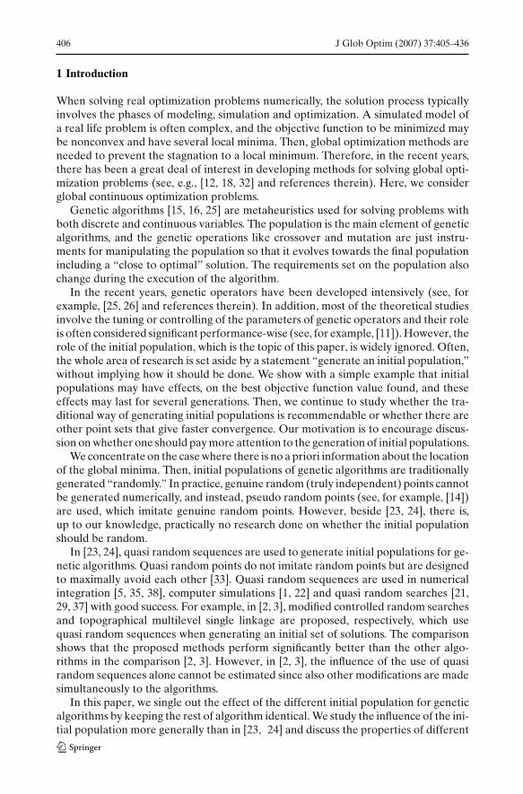
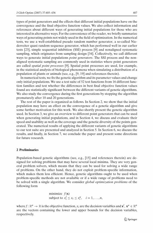
Figures 1 and 2 illustrate the convergence of a genetic algorithm for the 10-dimen-sional Griewangk function and 10-dimensional Katsuura function:

Griewangk function: f (x) =10∑

i=1

(x2i /4000) −

10∏

i=1

(cos(xi)/√

i) − 10 ≤ xi ≤ 100,

Katsuura function: f (x) =10∏

i=1

(1 + i

30∑

k=1

| 2kxi − ⌊2kxi

⌋ |2k

), −0.1 < xi < 1.

Each curve illustrates the average convergence for 100 separate runs of a geneticalgorithm. The three different curves in Figs. 1 and 2 correspond to runs with differ-ent initial populations generated by using a pseudo random number generator. Herepseudo stands for the case, where the initial pseudo random population is spreadout over the whole feasible region. Furthermore, clustered 1 and clustered 2 stand forcases where the initial population is restricted to a subspace of the feasible region. The

J Glob Optim (2007) 37:405–436 409

5 10 15 200

10

20

30

40

50

60

Generations

Bes

t obj

ectiv

e fu

nctio

n va

lue

foun

d clustered 1pseudoclustered 2

Fig. 1 The convergence of a genetic algorithm for 10D Griewangk function with different initialpopulations

40 45 50 55 600

500

1000

1500

2000

Generations

Bes

t obj

ectiv

e fu

nctio

n va

lue

foun

d clustered 1pseudoclustered 2

Fig. 2 The convergence of a genetic algorithm for 10D Katsuura function with different initialpopulations

subspace is defined by restricting each variable xi to the upper and lower 80% of theirtotal range for clustered 1 and clustered 2, respectively. For the Griewangk function thecurves merge after 30 generations. The Katsuura function requires more generationsand, therefore, also the curves merge later than for the Griewangk function. (Notethe different scales in Figs. 1 and 2.) For both Griewangk and Katsuura functions, thedifferences in the best objective function values found is quite significant when thenumber of generations is small. This indicates that the initial population has an effecton the convergence of a genetic algorithm.

The clustered populations used in the simple example above were only theoretical.In practice, such initial populations would hardly be used, unless there were some

410 J Glob Optim (2007) 37:405–436

a priori knowledge about the location of the global minima. The rest of the paperconcentrates on more realistic alternative ways for generating initial populations.

When there is no a priori information available on the location and the numberof local optima, then the initial population of a genetic algorithm should be able toreach as large part of the feasible region as possible by means of crossover. We callthis property genetic diversity, and it is related to the independence of points. Anotherdesirable property for an initial population is a good uniform coverage. By a gooduniform coverage we mean that the points are well spread out to cover the whole fea-sible region. Points have a good uniform coverage if they do not form clusters or leaverelatively large areas of the feasible region unexplored. A good uniform coverage isdesired, because then information is obtained throughout the whole feasible region.This helps to prevent premature convergence.

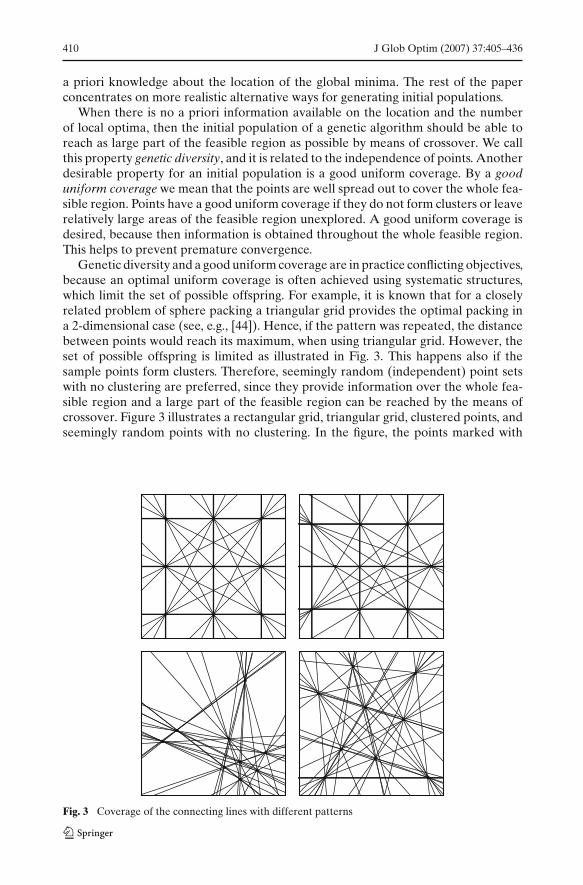
Genetic diversity and a good uniform coverage are in practice conflicting objectives,because an optimal uniform coverage is often achieved using systematic structures,which limit the set of possible offspring. For example, it is known that for a closelyrelated problem of sphere packing a triangular grid provides the optimal packing ina 2-dimensional case (see, e.g., [44]). Hence, if the pattern was repeated, the distancebetween points would reach its maximum, when using triangular grid. However, theset of possible offspring is limited as illustrated in Fig. 3. This happens also if thesample points form clusters. Therefore, seemingly random (independent) point setswith no clustering are preferred, since they provide information over the whole fea-sible region and a large part of the feasible region can be reached by the means ofcrossover. Figure 3 illustrates a rectangular grid, triangular grid, clustered points, andseemingly random points with no clustering. In the figure, the points marked with

Fig. 3 Coverage of the connecting lines with different patterns

J Glob Optim (2007) 37:405–436 411

small black dots are parent solutions and the lines running through them illustrate allthe possible locations of offsprings.

3 Generating initial population

Many sub-areas of genetic algorithms have been studied elaborately, but the selectionof an initial population has been widely ignored. As mentioned earlier, the traditionalway to generate the initial population is to use pseudo random numbers, and morerecently also quasi random sequences have been applied in [23, 24]. Pseudo randomnumbers imitate genuine random numbers and quasi random sequences are designedto produce points that maximally avoid each other.

Pseudo random initial populations can be generated in numerous ways. The mainclasses are congruential and recursive generators. Common congruential generatorsinclude linear, quadratic, inversive, additive and parallel linear congruential genera-tors [14, 45]. Recursive generators include multiplicative recursive, lagged Fibonacci,multiply-with-carry-generator, add-with-carry and substract-with-borrow generators[14]. There are also pseudo random vector generators, which produce sequences ofvectors instead of scalars. Examples of those are feedback shift register generator [14]and SQRT generator [43].

Common quasi random sequence generators include Van der Corput, Hammers-ley, Halton, Faure, Sobol’ and Niederreiter generators [4, 14, 30]. For the convenienceof the reader some examples of both pseudo random number generators and quasirandom sequence generators are included in the Appendix along with further refer-ences.

Pseudo random numbers and quasi random sequences are quite well-known forresearchers in optimization, but there are also other types of point generators. Spatialpoint processes are commonly used in statistics but they are less well-known in opti-mization. Therefore, we now shortly describe the spatial point processes used in thispaper.

3.1 Spatial point processes

Spatial point processes [9] can be considered to be transformations of pseudo randompoint initialization which lead to a good uniform coverage and simultaneously avoidperiodicity in the configuration generated.

Some spatial point processes include a parameter, by which the proportion of thetwo conflicting properties, genetic diversity and a good uniform coverage, can be con-trolled. Hence, the same process can be used to generate genetically diverse points orpoints with a good uniform coverage or something in between.

There are several types of spatial point processes. For our purposes, it is ade-quate to differentiate between clustering and inhibition processes. Clustering pro-cesses generate points that simulate populations, where the individuals tend to formclusters. However, we are more interested in the situation where each individualis as far apart as possible from the adjacent individuals resulting in an evenly dis-tributed population without clusters. Therefore, we concentrate on inhibition pro-cesses, where an individual (a point) is either explicitly prohibited to be locatedcloser than some predefined minimum distance � > 0 to the other individuals, orindividuals are kept apart by some implicit means. We describe here two inhibition

412 J Glob Optim (2007) 37:405–436

processes: a simple sequential inhibition process and a nonaligned systematicsampling.

Simple sequential inhibition process: In the simple sequential inhibition (SSI)process [9], a new individual is accepted to enter the population only if its distance toall the existing individuals in the population is at least �.

In the following pseudo code for the SSI process the parameter population size isthe number of points to be generated, futile is the number of rejected trial points dur-ing the current iteration, Max_futile is the maximum number of rejected trial pointsin one iteration before terminating the process, and n is the dimension of the spacewhere the points are generated.

0. Initialize parameters population size, Max_futile and dimension n and set futile = 0and k = 0.

1. Do until k == population size or futile==Max_futile1.1 Generate a trial point.

(Use a pseudo or a quasi random number generator to generate a trial pointto the n-dimensional unit hyper cube.)

1.2 Check whether the trial point is accepted.If the distance to the existing individuals is larger than �, accept the pointinto the population, and set k = k + 1 and futile= 0.Else, set futile = futile+1.

End do

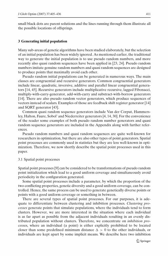
The distance between points can be computed using different metrics. If the minimumdistance � is defined to be too large, then the maximum number of rejected trial pointsin one iteration is reached and the process is terminated prematurely. In that case, wesupplement the sample with pseudo random points to match the population size.Nonaligned systematic sampling: In the nonaligned systematic sampling, which orig-inates from sampling design [34], the unit hyper cube is divided into bn elementaryintervals (see Appendix) with equal side lengths (i.e., an equally spaced grid). Thenone sample point is selected from each elementary interval according to prescribedrules. Nonaligned systematic sampling uses b · n pseudo random numbers to definethe location of the sample points. In two dimensions, the sample points are generatedusing the formula

x = ([(j − 1) + ri,1]�, [(i − 1) + rj,2]�),

where i, j = 1, . . . , b, � = 1/b, and r is a b × n array of pseudo random numbers, seeFig. 4. In the following pseudo code for an n-dimensional case of the nonaligned sys-tematic sampling, v is a vector of auxiliary integer variables. It is used to determine thecorrect elementary interval and the correct pseudo random number when calculatingthe nonaligned systematic sample points x.

0. Initialize vj = 0 for j = 0, . . . , n − 1, and the b × n pseudo random number array r.1. Do i = 0, . . . , bn − 1.

1.1 Compute sample point xi

Do j = 0, . . . , n − 1 // Compute the jth component of xi

S = (∑nk=1 vk

) − vjl = (S)mod b

xij = (rl, j + vj)�

End do

J Glob Optim (2007) 37:405–436 413

Fig. 4 Nonaligned systematicsampling points in twodimensions

1.2 Update vDo j = 0, . . . , n − 1

If ((i)mod bj == bj − 1) then vj = (vj + 1)mod bEnd do

End do

Note that the number of nonaligned systematic sampling points cannot be chosenfreely, but is determined by the grid size and the dimension. In practice, when a cer-tain number of sample points is required, we supplement the nonaligned systematicsample with pseudo random points to match the required number of points.

4 Properties of point generators

In this section, we consider the distribution and the genetic diversity of the pointsgenerated by pseudo random number generators, quasi random sequence generatorsand spatial point processes. We also consider the speed and the usability of somespecific generators. We are interested in point sets with a relatively small number ofpoints since the number of points generated equals the population size and rangestypically from tens to a few hundreds.

In the illustrations and numerical examples of point generation, we have selectedgood representatives for the different types of point generators. The pseudo randomnumber generator is a multiplicative linear congruential generator from the well-established numerical library of the Numerical Algorithms Group Ltd (NAG) andthe quasi random sequence generator is the Niederreiter generator [30] that hasproved successful in our earlier tests [23, 24]. The representatives of spatial pointprocesses are the SSI process and the nonaligned systematic sampling. In the SSI pro-cess, the trial points are generated using the Niederreiter generator and the distancesare measured using L2-metric. The nonaligned systematic sampling is as defined inSection 3.

The properties of the point generators are described in the following four sub-sections and the results are summarized and some conclusions are drawn in the fifthsubsection.

414 J Glob Optim (2007) 37:405–436

4.1 Distribution

Intuitively thinking, it is beneficial if no large areas are left unexplored when samplingindividuals for an initial population of a genetic algorithm. The point generators pre-sented in Section 3 produce point clouds with a degree of uniform coverage. However,there are differences in how well the points of these sequences are spread out. In opti-mization and in numerical integration, the goodness of the uniform coverage of apoint set is commonly measured by discrepancy or dispersion [30]. Here, we give thedefinition for the discrepancy.

Discrepancy Let In ⊂ Rn be an n-dimensional unit hyper cube, let P be a set consist-ing of points x1, ..., xN ∈ In, and let B be a nonempty family of Lebesgue-measurablesubintervals of In and B ∈ B. Furthermore, let A(B; P) be a counting function definedas the number of points xk, 1 ≤ k ≤ N, for which xk ∈ B. Then, discrepancy DN

with respect to P in In is defined as DN(B; P) = supB∈B∣∣∣A(B;P)

N − λ(B)

∣∣∣ , where λ is a

Lebesgue-measure.

Discrepancy is large, when there exists clusters or large unexplored areas. Hence,we are interested in point sets that have low values for discrepancy. A mathematicalrelationship between discrepancy and dispersion is given in [30], and it shows thatevery low-discrepancy sequence is also a low-dispersion sequence, but not vice versa.

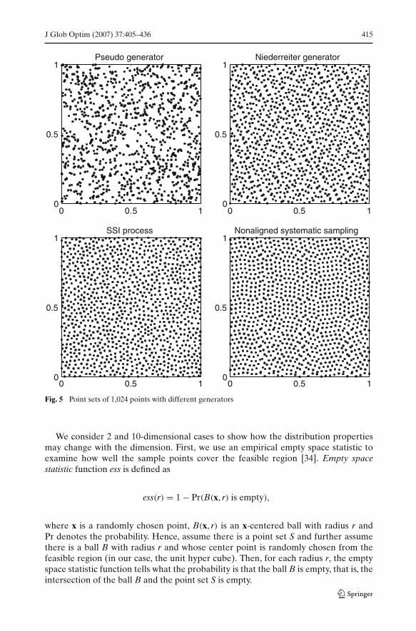
Quasi random sequences are also called low-discrepancy sequences. Their discrep-ancy value for a large sample size N is of order of magnitude C(logN)nN−1, whereC is a generator-specific coefficient depending only on the dimension n [27]. This isalso a minimum possible discrepancy size for large N (see, e.g., [27]). The boundsfor discrepancy, however, are relevant only for a very large number of sample pointsas used in numerical integration. When generating only initial populations, we aremore interested in the distribution of a small number of points. Some quasi randomsequences have the property that the first bm successive points divide evenly on thecorresponding elementary intervals (see Appendix). This indicates that quasi randomsequences may have good discrepancy values also for small sample sizes. Figure 5 illus-trates four two-dimensional initial populations with 1,024 individuals generated usingthe multiplicative linear congruential (pseudo) generator, the Niederreiter generator,the SSI process and the nonaligned systematic sampling, respectively.

In Fig. 5, we see that pseudo random points form clusters and leave some areasrelatively unexplored, whereas the other samples cover the feasible region quite well.However, quasi random sequences may sometimes form point patterns, whose dis-tribution properties depend on the number of points generated. Then, at a certainnumber of sample points the pattern may be unfavorable for optimization purposes.An example of this behavior is illustrated in Fig. 6, where again 1,024 points were gen-erated with a slightly different configuration. For more information on the distributionof different quasi random sequences, we refer to [27].

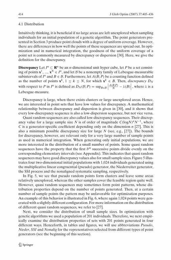
Next, we consider the distribution of small sample sizes. In optimization withgenetic algorithms we used a population of 201 individuals. Therefore, we next empir-ically examine the distribution properties of sets with 201 points generated in fourdifferent ways. Henceforth, in tables and figures, we will use abbreviations Pseudo,Nieder, SSI and Nonalig for the representatives selected from different types of pointgenerators (see the beginning of this section).

J Glob Optim (2007) 37:405–436 415

0 0.5 10

0.5

1Pseudo generator

0 0.5 10

0.5

1Niederreiter generator

0 0.5 10

0.5

1SSI process

0 0.5 10

0.5

1Nonaligned systematic sampling

Fig. 5 Point sets of 1,024 points with different generators

We consider 2 and 10-dimensional cases to show how the distribution propertiesmay change with the dimension. First, we use an empirical empty space statistic toexamine how well the sample points cover the feasible region [34]. Empty spacestatistic function ess is defined as

ess(r) = 1 − Pr(B(x, r) is empty),

where x is a randomly chosen point, B(x, r) is an x-centered ball with radius r andPr denotes the probability. Hence, assume there is a point set S and further assumethere is a ball B with radius r and whose center point is randomly chosen from thefeasible region (in our case, the unit hyper cube). Then, for each radius r, the emptyspace statistic function tells what the probability is that the ball B is empty, that is, theintersection of the ball B and the point set S is empty.

416 J Glob Optim (2007) 37:405–436

Fig. 6 Another example of1,024 points generated with theNiederreiter generator

0 0.5 10

0.5

1Niederreiter generator

To experimentally define the empty space statistic functions for each point set con-taining 201 points, we generated 10,000 auxiliary pseudo random points1 on a unithyper cube and for each of the 10,000 auxiliary points calculated the maximal radiusr so that B(x, r) is empty, that is, does not contain any of the 201 points under consid-eration. We did this in both 2- and 10-dimensional cases for the four different pointsets.

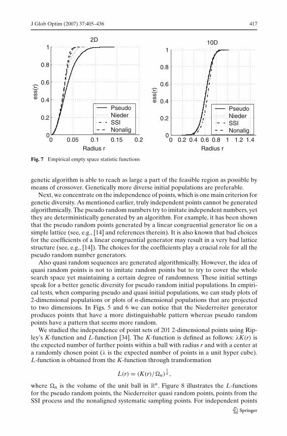
The empirical empty space statistic functions are illustrated in Fig. 7. For us, theimportant property of the empty space statistic function is the steepness of the curve(the steeper the better). If the curve is steep, it indicates that if a random ball withradius r is selected from the unit hyper cube, then whether the ball is empty dependsmainly on the radius—not the location of the ball. If, on the other hand, the curve isgentle, the emptiness of the ball depends strongly on the location, hence the point setis not evenly distributed.

The empirical empty space statistic functions show that in two dimensions, the non-aligned systematic sampling and the simple sequential inhibition (SSI) process providethe best coverages closely followed by the Niederreiter quasi random sequence gen-erator. The pseudo random initial population has clearly the worst coverage, whichconfirms the findings earlier shown in Fig. 5. However, in ten dimensions the differ-ences diminish, because the populations become sparse. The only notable differenceis that for the population generated with the SSI process the curve of the empiricalempty space statistic function is now below the other curves with the small values ofr but rises more steeply in the end. This indicates better coverage for the SSI process.

4.2 Genetic diversity

The population of a genetic algorithm evolves largely by crossovers and mutations. Inour implementation, the most dominant genetic operator is crossover, since it usuallychanges the solutions most. We define genetic diversity as a property by which the

1 Here, we naturally used a different pseudo random number generator than when generating theinitial population. To make sure that the use of pseudo random numbers did not bias the results wealso computed the empty space statistic functions using a grid of 10,000 points, which led to similarresults.

J Glob Optim (2007) 37:405–436 417

0 0.05 0.1 0.15 0.20

0.2

0.4

0.6

0.8

1

Radius r

ess(

r)2D

PseudoNiederSSINonalig

0 0.2 0.4 0.6 0.8 1 1.2 1.40

0.2

0.4

0.6

0.8

1

Radius res

s(r)

10D

PseudoNiederSSINonalig

Fig. 7 Empirical empty space statistic functions

genetic algorithm is able to reach as large a part of the feasible region as possible bymeans of crossover. Genetically more diverse initial populations are preferable.

Next, we concentrate on the independence of points, which is one main criterion forgenetic diversity. As mentioned earlier, truly independent points cannot be generatedalgorithmically. The pseudo random numbers try to imitate independent numbers, yetthey are deterministically generated by an algorithm. For example, it has been shownthat the pseudo random points generated by a linear congruential generator lie on asimple lattice (see, e.g., [14] and references therein). It is also known that bad choicesfor the coefficients of a linear congruential generator may result in a very bad latticestructure (see, e.g., [14]). The choices for the coefficients play a crucial role for all thepseudo random number generators.

Also quasi random sequences are generated algorithmically. However, the idea ofquasi random points is not to imitate random points but to try to cover the wholesearch space yet maintaining a certain degree of randomness. These initial settingsspeak for a better genetic diversity for pseudo random initial populations. In empiri-cal tests, when comparing pseudo and quasi initial populations, we can study plots of2-dimensional populations or plots of n-dimensional populations that are projectedto two dimensions. In Figs. 5 and 6 we can notice that the Niederreiter generatorproduces points that have a more distinguishable pattern whereas pseudo randompoints have a pattern that seems more random.

We studied the independence of point sets of 201 2-dimensional points using Rip-ley’s K-function and L-function [34]. The K-function is defined as follows: λK(r) isthe expected number of further points within a ball with radius r and with a center ata randomly chosen point (λ is the expected number of points in a unit hyper cube).L-function is obtained from the K-function through transformation

L(r) = (K(r)/�n)1n ,

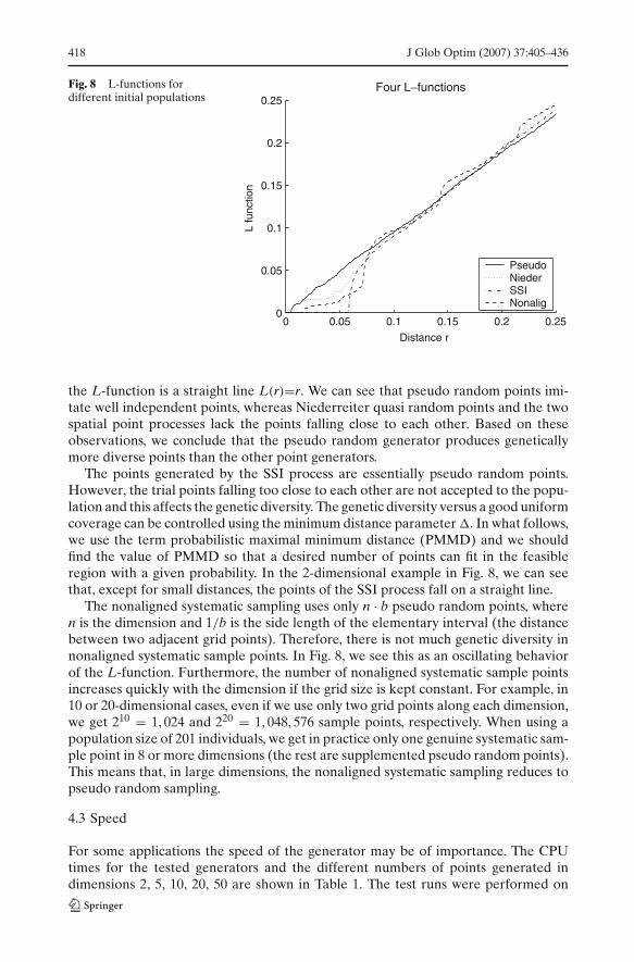
where �n is the volume of the unit ball in Rn. Figure 8 illustrates the L-functions

for the pseudo random points, the Niederreiter quasi random points, points from theSSI process and the nonaligned systematic sampling points. For independent points

418 J Glob Optim (2007) 37:405–436

Fig. 8 L-functions fordifferent initial populations

0 0.05 0.1 0.15 0.2 0.250

0.05

0.1

0.15

0.2

0.25Four L−functions

Distance r

L fu

nctio

n

PseudoNiederSSINonalig

the L-function is a straight line L(r)=r. We can see that pseudo random points imi-tate well independent points, whereas Niederreiter quasi random points and the twospatial point processes lack the points falling close to each other. Based on theseobservations, we conclude that the pseudo random generator produces geneticallymore diverse points than the other point generators.

The points generated by the SSI process are essentially pseudo random points.However, the trial points falling too close to each other are not accepted to the popu-lation and this affects the genetic diversity. The genetic diversity versus a good uniformcoverage can be controlled using the minimum distance parameter �. In what follows,we use the term probabilistic maximal minimum distance (PMMD) and we shouldfind the value of PMMD so that a desired number of points can fit in the feasibleregion with a given probability. In the 2-dimensional example in Fig. 8, we can seethat, except for small distances, the points of the SSI process fall on a straight line.

The nonaligned systematic sampling uses only n · b pseudo random points, wheren is the dimension and 1/b is the side length of the elementary interval (the distancebetween two adjacent grid points). Therefore, there is not much genetic diversity innonaligned systematic sample points. In Fig. 8, we see this as an oscillating behaviorof the L-function. Furthermore, the number of nonaligned systematic sample pointsincreases quickly with the dimension if the grid size is kept constant. For example, in10 or 20-dimensional cases, even if we use only two grid points along each dimension,we get 210 = 1, 024 and 220 = 1, 048, 576 sample points, respectively. When using apopulation size of 201 individuals, we get in practice only one genuine systematic sam-ple point in 8 or more dimensions (the rest are supplemented pseudo random points).This means that, in large dimensions, the nonaligned systematic sampling reduces topseudo random sampling.

4.3 Speed

For some applications the speed of the generator may be of importance. The CPUtimes for the tested generators and the different numbers of points generated indimensions 2, 5, 10, 20, 50 are shown in Table 1. The test runs were performed on

J Glob Optim (2007) 37:405–436 419

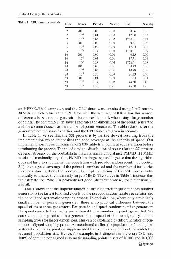
Table 1 CPU times in seconds Dim Points Pseudo Nieder SSI Nonalig

2 201 0.00 0.00 0.06 0.002 104 0.01 0.00 17.60 0.022 105 0.06 0.02 1774.0 0.235 201 0.00 0.00 0.2 0.005 104 0.02 0.00 17.84 0.065 105 0.14 0.03 1760.0 0.67

10 201 0.00 0.00 0.23 0.0010 104 0.03 0.01 17.71 0.0410 105 0.28 0.05 1773.0 0.9820 201 0.00 0.01 0.73 0.0020 104 0.06 0.01 10.78 0.0520 105 0.55 0.09 21.33 0.4650 201 0.01 0.00 1.54 0.0150 104 0.14 0.02 44.50 0.1250 105 1.38 0.2 45.68 1.2

an HP9000/J5600 computer, and the CPU times were obtained using NAG routineX05BAF, which returns the CPU time with the accuracy of 0.01 s. For this reason,differences between some generators become evident only when using a large numberof points. The column Dim in Table 1 indicates the dimensions of the points generatedand the column Points lists the number of points generated. The abbreviations for thegenerators are the same as earlier, and the CPU times are given in seconds.

In Table 1, we see that the SSI process is by far the slowest resulting from theimplementation which emphasizes the good coverage at the expense of speed. Ourimplementation allows a maximum of 2,000 futile trial points at each iteration beforeterminating the process. The speed (and the distribution of points) for the SSI processdepends strongly on the probabilistic maximal minimum distance PMMD. If PMMDis selected maximally large (i.e., PMMD is as large as possible yet so that the algorithmdoes not have to supplement the population with pseudo random points, see Section3.1), then a good coverage of the points is emphasized and the number of futile triesincreases slowing down the process. Our implementation of the SSI process auto-matically estimates the maximally large PMMD. The values in Table 1 indicate thatthe estimate for PMMD is probably not good (distribution-wise) for dimensions 20and 50.

Table 1 shows that the implementation of the Niederreiter quasi random numbergenerator is the fastest followed closely by the pseudo random number generator andthe nonaligned systematic sampling process. In optimization, where only a relativelysmall number of points is generated, there is no practical difference between thespeed of these three generators. For pseudo and quasi random number generatorsthe speed seems to be directly proportional to the number of points generated. Wecan see that, compared to other generators, the speed of the nonaligned systematicsampling grows for larger dimensions. This can be explained by different ratios of gen-uine nonaligned sampling points. As mentioned earlier, the population of nonalignedsystematic sampling points is supplemented by pseudo random points to match therequired population size. Hence, for example, in 5 dimensions there are 78% and100% of genuine nonaligned systematic sampling points in sets of 10,000 and 100,000

420 J Glob Optim (2007) 37:405–436

sample points, respectively, whereas in 10 dimensions the respective values are only10% and 59%. In 20 dimensions, all except one sample point are already random evenif the sample size was as large as one million (220 > 106).

4.4 Usability

In this section, we discuss the usability of different number generators. Some fea-tures affecting usability have already been mentioned earlier and are summarizedhere.

Pseudo random number generators are by far the most commonly used ones inoptimization. The greatest advantage of pseudo random number generators concern-ing usability is that there exist implementations that are well-established, well-testedand easily available. However, a good random-like behavior is not a matter-of-course,but requires a careful choice of parameters, that is, coefficients and seeds (or initialsequences). As earlier noted for linear congruential generators, wrong choices forparameter values may cause the points in a sequence to be badly distributed. Thisis true for other generators as well. Many of the pseudo random number generatorsare easy to implement, but the analysis of the distribution is difficult, especially foran arbitrary seed (or arbitrary initial sequences). According to [14], only well-testedpseudo random generators should be used. These generators often use fixed coeffi-cients and sometimes limit the choice of seeds (or initial sequences). This is one way tosecure good distribution properties, assuming those values are tested and approved.

Contrary to pseudo random number generators, quasi random number generatorsare neither so well-established, well-tested nor easily available. On the other hand,quasi random number generators having solid theoretical properties do not need somuch numerical testing. The use of available quasi generators is easy and the quasirandom points are guaranteed to have some advantageous properties as described inthe Appendix. Quasi generators provide the same sequences on different runs of thegenerator and, hence, they do not require a seed or an initial sequence from the user.Since quasi generators take into consideration the location of the previous points,they also expect that the sequence is started from the beginning. These two propertiesmake quasi generators easier to use, because the user only has to give the numberof points to be generated and the dimension as parameters. At the same time, theseproperties may become a disadvantage if the user for some reason wants to obtaindifferent sequences in the same dimension. On this occasion, the easiest way outmight be to generate points in higher dimensions and then project them to the desireddimension, but this may have an effect on the distribution properties.

The SSI process is not commonly available for an n-dimensional case, but theimplementation is straightforward given that the user provides the PMMD value.However, it gets more complicated if the user provides only the number of points tobe generated and the optimal PMMD (with respect to the coverage) must be estimatedautomatically. This issue is discussed in more detail in Section 6. An interesting prop-erty of the SSI process is that the proportion of the two conflicting objectives, that is,the genetic diversity and the good uniform coverage, can both be controlled using theprobabilistic maximal minimum distance parameter PMMD. Note that, if desired, theSSI process provides different points on every run just like pseudo random numbergenerators.

The nonaligned systematic sampling processes are not commonly available inn-dimensions, but they are easy to implement and to use. However, when

J Glob Optim (2007) 37:405–436 421

generating a relatively small number of points, it is practical to use the systematicsampling process only in small dimensions. Otherwise, the proportion of genuinenonaligned systematic sample points is small. This is a strong limitation in the area ofoptimization.

4.5 Summary of features

An ideal generator for our purposes should generate well-distributed, geneticallydiverse points in n-dimensions, and it should be relatively fast and easy to use. InTable 2, we summarize the evaluation made in this section. The evaluation of differ-ent point generators has been marked using plus signs (+): the more plus signs thebetter the score. In case of a notable difference in how well a generator works forproblems with small and large dimensions (here small denotes less than, say, five), theoccasions are scored separately (small/large). For example, the nonaligned systematicsampling scores +++/+ in coverage, which means that it works well in small dimensionsand poorly in large dimensions.

Note that only coverage and genetic diversity may have a direct influence on objec-tive function values in optimization since they are the properties of the points whereasspeed and usability are properties of the generators. Considering just the propertiesof the points we notice in Table 2 that pseudo random points have good genetic diver-sity, but the worst coverage, and the SSI process produces points with good coverage,but only average genetic diversity. The properties of the Niederreiter quasi randompoints settle somewhere between pseudo and the SSI process. In the further analysis,we pay less attention to the nonaligned systematic sampling since it is not applica-ble for problems with several variables. To find out the effects of the coverage andgenetic diversity, we concentrate on the pseudo random number generator and theSSI process.

5 Experimentations

We test the influence of initial populations computationally by using different pointgenerators and a large number of difficult test problems from the literature. The influ-ence of the different initial populations is analyzed after 10 and 20 generations andafter the execution of the whole algorithm. The genetic algorithm used is presentedin Section 2.

5.1 Test settings

The test runs were performed on an HP9000/J5600 computer. We solved a test suite of52 problems using genetic algorithms described in Section 2 with the parameter values

Table 2 Summary ofgenerator properties

Properties (small/large) Pseudo Nieder SSI Nonalig

Coverage + ++ +++ +++/+Genetic diversity +++ ++ ++ +Speed +++ +++ + ++/+++Usability +++ +++ ++ +++/+

422 J Glob Optim (2007) 37:405–436

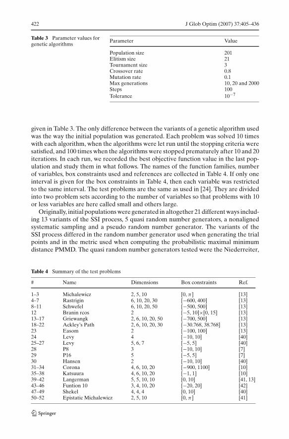
Table 3 Parameter values forgenetic algorithms

Parameter Value

Population size 201Elitism size 21Tournament size 3Crossover rate 0.8Mutation rate 0.1Max generations 10, 20 and 2000Steps 100Tolerance 10−7

given in Table 3. The only difference between the variants of a genetic algorithm usedwas the way the initial population was generated. Each problem was solved 10 timeswith each algorithm, when the algorithms were let run until the stopping criteria weresatisfied, and 100 times when the algorithms were stopped prematurely after 10 and 20iterations. In each run, we recorded the best objective function value in the last pop-ulation and study them in what follows. The names of the function families, numberof variables, box constraints used and references are collected in Table 4. If only oneinterval is given for the box constraints in Table 4, then each variable was restrictedto the same interval. The test problems are the same as used in [24]. They are dividedinto two problem sets according to the number of variables so that problems with 10or less variables are here called small and others large.

Originally, initial populations were generated in altogether 21 different ways includ-ing 13 variants of the SSI process, 5 quasi random number generators, a nonalignedsystematic sampling and a pseudo random number generator. The variants of theSSI process differed in the random number generator used when generating the trialpoints and in the metric used when computing the probabilistic maximal minimumdistance PMMD. The quasi random number generators tested were the Niederreiter,

Table 4 Summary of the test problems

# Name Dimensions Box constraints Ref.

1–3 Michalewicz 2, 5, 10 [0, π ] [13]4–7 Rastrigin 6, 10, 20, 30 [−600, 400] [13]8–11 Schwefel 6, 10, 20, 50 [−500, 500] [13]12 Branin rcos 2 [−5, 10]×[0, 15] [13]13–17 Griewangk 2, 6, 10, 20, 50 [−700, 500] [13]18–22 Ackley’s Path 2, 6, 10, 20, 30 [−30.768, 38.768] [13]23 Easom 2 [−100, 100] [13]24 Levy 4 [−10, 10] [40]25–27 Levy 5, 6, 7 [−5, 5] [40]28 P8 3 [−10, 10] [7]29 P16 5 [−5, 5] [7]30 Hansen 2 [−10, 10] [40]31–34 Corona 4, 6, 10, 20 [−900, 1100] [10]35–38 Katsuura 4, 6, 10, 20 [−1, 1] [10]39–42 Langerman 5, 5, 10, 10 [0, 10] [41, 13]43–46 Funtion 10 3, 4, 10, 20 [−20, 20] [42]47–49 Shekel 4, 4, 4 [0, 10] [40]50–52 Epistatic Michalewicz 2, 5, 10 [0, π ] [41]

J Glob Optim (2007) 37:405–436 423

Faure and Halton generator and two variants of the Sobol’ generator. The numericalresults of the genetic algorithm with quasi random initial populations are reportedin [23], where the Niederreiter generator performed the best. Here, we report theresults of the genetic algorithm using initial populations generated by the good rep-resentatives from different types of point generators (see the beginning of Section4).

5.2 Numerical results

In this subsection, we present the results of the experiments described above. In whatfollows, we consider only the best objective function values that the algorithm hasfound (in the last population) and pay attention to the average and variance of thesevalues in the repeated runs.

Let us first consider those tests where the genetic algorithm was run until a stoppingcriterion was satisfied. Table 5 shows the average final objective function values f (x)

and the average standard deviations σ(f ) for small and large problems. As we can see,for small problems, in the average objective function values, there are no differences inthree significant digits. However, for large problems the differences in average objec-tive function values are quite large. Based solely on the average objective functionvalues in Table 5 one could draw the conclusion that nonaligned systematic samplesand Niederreiter quasi random points are clearly the most suitable for initial popula-tions. This, however, is not completely true as our further analysis reveals, when weconsider also the variances.

Before any statistical tests, we make an observation on the results in Table 5. Asmentioned in Section 4.2, nonaligned systematic sampling reduces to pseudo randomsampling for large problems. However, the average objective function value and theaverage standard deviation of those algorithms differ quite remarkably for large prob-lems. This indicates that the average values are not good measures in the comparison.

We applied analysis of variance (ANOVA) to the final objective function values tofind out whether the differences were statistically significant. The analysis of varianceindicated that only in 4 out of 52 test problems there were statistically significantdifferences (with 95% confidence). We call these four problems critical problems, andthey are the problems 40, 49, 51 and 52 in Table 4. Surprisingly, all the critical prob-lems were small (problems with 10 or less variables). This can be explained by thesmall variance for these problems. The fact that there was no statistically significantdifference in the objective function values for any of the large problems is explainedby their very large variances. The variances were the largest for the 20-dimensionalKatsuura problem for which the variances were 8,473, 2,060, 509 and 17,100 for thepseudo, Niederreiter, SSI and nonaligned, respectively. The 20-dimensional Katsuura

Table 5 Average objectivefunction values and standarddeviations for small and largeproblems

Pseudo Nieder SSI Nonalig

f (x) Small −186.7 −186.7 −186.8 −186.6f (x) Large −1896.0 −2205.4 −1680.2 −2295.9σ(f ) Small 0.34 0.28 0.37 0.58σ(f ) Large 885.9 355.3 162.5 1697.9

424 J Glob Optim (2007) 37:405–436

problem biased the average values in Table 5 and was the main cause of differencesfor large problems.

Next, we study the critical problems more closely. Figure 9 shows the averageobjective function values for the four critical problems. Ps, Ni, SSI and No stand forthe pseudo, Niederreiter, SSI process and nonaligned systematic sampling, respec-tively, and the whiskers illustrate the standard deviations. In addition, the P valuesrelated to the F test of ANOVA [28] are given in the parenthesis subsequent to theproblem number. The four plots reveal that there is no overall dominance betweenthe genetic algorithm variants, however the variant applying quasi random points per-formed best in 3 out of 4 cases and also points generated by the SSI process performedbetter than pseudo random points in 3 out of 4 instances. Nonaligned systematic sam-pling performed very similarly to pseudo random points in three cases and was betterin one.

So far we have studied the differences in objective function values after runningthe whole algorithm and there has been only minor differences. Next, we consideralso the situations, where the algorithm is stopped prematurely after 10 and 20 gener-ations. Earlier, we noticed difficulties in interpreting values that were not scaled: onelarge value could strongly bias the results. Therefore, we now define a more reliablemeasure of performance by scaling the objective function values to the range from 0to 1. Scaled average objective function value sf is defined as follows

sf = f − f min

f max − f min

,

Ps Ni SSI No-1

-0.8

-0.6

Problem 40 (P=0.007)

Ps Ni SSI No

-14

-10

-6

-2

Problem 49 (P=0.040)

Ps Ni SSI No-4.7

-4.6

-4.5

Problem 51 (P=0.001)

Ps Ni SSI No

-9.6

-9.2

-8.8Problem 52 (P=0.043)

Fig. 9 Average objective function values and standard deviations

J Glob Optim (2007) 37:405–436 425

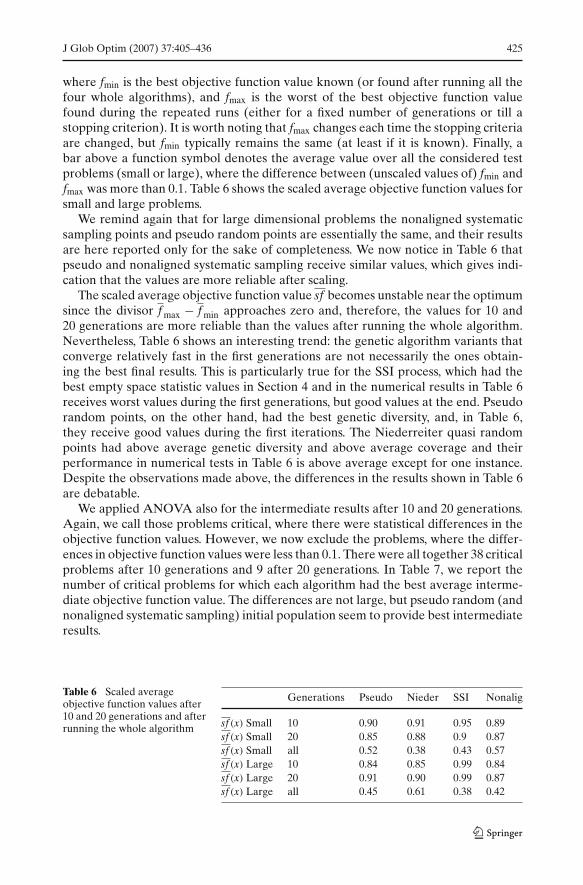
where fmin is the best objective function value known (or found after running all thefour whole algorithms), and fmax is the worst of the best objective function valuefound during the repeated runs (either for a fixed number of generations or till astopping criterion). It is worth noting that fmax changes each time the stopping criteriaare changed, but fmin typically remains the same (at least if it is known). Finally, abar above a function symbol denotes the average value over all the considered testproblems (small or large), where the difference between (unscaled values of) fmin andfmax was more than 0.1. Table 6 shows the scaled average objective function values forsmall and large problems.

We remind again that for large dimensional problems the nonaligned systematicsampling points and pseudo random points are essentially the same, and their resultsare here reported only for the sake of completeness. We now notice in Table 6 thatpseudo and nonaligned systematic sampling receive similar values, which gives indi-cation that the values are more reliable after scaling.

The scaled average objective function value sf becomes unstable near the optimumsince the divisor f max − f min approaches zero and, therefore, the values for 10 and20 generations are more reliable than the values after running the whole algorithm.Nevertheless, Table 6 shows an interesting trend: the genetic algorithm variants thatconverge relatively fast in the first generations are not necessarily the ones obtain-ing the best final results. This is particularly true for the SSI process, which had thebest empty space statistic values in Section 4 and in the numerical results in Table 6receives worst values during the first generations, but good values at the end. Pseudorandom points, on the other hand, had the best genetic diversity, and, in Table 6,they receive good values during the first iterations. The Niederreiter quasi randompoints had above average genetic diversity and above average coverage and theirperformance in numerical tests in Table 6 is above average except for one instance.Despite the observations made above, the differences in the results shown in Table 6are debatable.

We applied ANOVA also for the intermediate results after 10 and 20 generations.Again, we call those problems critical, where there were statistical differences in theobjective function values. However, we now exclude the problems, where the differ-ences in objective function values were less than 0.1. There were all together 38 criticalproblems after 10 generations and 9 after 20 generations. In Table 7, we report thenumber of critical problems for which each algorithm had the best average interme-diate objective function value. The differences are not large, but pseudo random (andnonaligned systematic sampling) initial population seem to provide best intermediateresults.

Table 6 Scaled averageobjective function values after10 and 20 generations and afterrunning the whole algorithm

Generations Pseudo Nieder SSI Nonalig

sf (x) Small 10 0.90 0.91 0.95 0.89sf (x) Small 20 0.85 0.88 0.9 0.87sf (x) Small all 0.52 0.38 0.43 0.57sf (x) Large 10 0.84 0.85 0.99 0.84sf (x) Large 20 0.91 0.90 0.99 0.87sf (x) Large all 0.45 0.61 0.38 0.42

426 J Glob Optim (2007) 37:405–436

Table 7 The number ofproblems with best averageobjective function values forcritical problems

Generations Pseudo Nieder SSI Nonalig Total

10 9 9 8 12 3820 5 1 0 3 9

Before summarizing the results, let us yet consider the magnitudes of the variancesin the best objective function values separately from the actual objective functionvalues. In Table 8 are reported the number of test problems for which each algorithmhad the smallest variance after 10 and 20 generations and after running the wholealgorithms. We have excluded the problems where the differences in variances wereless than 0.1. The total number of problems considered is reported in the last columnof Table 8. It is noteworthy that the variant of genetic algorithm using pseudo randomnumbers has most often the smallest variance for the intermediate solutions, whichwas not expected.

5.3 Summary of numerical results

Here, we summarize the analysis made above. When considering final and intermedi-ate average objective function values, the analysis of variance indicated four criticalproblems for the final results and many more for the intermediate results where therewere significant differences in the best objective function values found. None of themethods clearly dominated the others, but in the scaled objective function values therewas a noticeable trend, namely that pseudo random initial populations provided onthe average good intermediate results, but not so good final results. The converse wastrue for the SSI process and quasi random points with better uniform coverage. Ear-lier we noticed that some clusterizations were harmful and some beneficial. Hence,genetic algorithms using pseudo random numbers and the variants where the initialpopulations have better uniform coverage performed in a slightly different way. Nev-ertheless, the differences, in general, were debatable and no strong conclusions couldbe made.

As far as the magnitudes of variances in the intermediate results are concerned,in most of the cases, the variance was the smallest for the genetic algorithm usingpseudo random numbers. There may be both harmful and beneficial clusterizationsas seen in Figs. 1 and 2. Harmful clusterizations lead to inferior and beneficial lead tosuperior objective function values compared to initial populations without clustering.One could have expected this to imply more significant differences in the magnitudesof variances in the early generations but this did not happen. However, again, noneof the algorithms clearly dominated the others and the differences were not large.

Finally, there were no significant differences in the magnitudes of variances relatedto final objective function values when applying clustered or unclustered initial popu-

Table 8 Number of testproblems when the variancewas smallest

Generations Pseudo Nieder SSI Nonalig Total

10 18 11 8 9 4620 12 11 6 15 44Final 5 9 3 2 19

J Glob Optim (2007) 37:405–436 427

lations. This could be assumed keeping in mind the observation that genetic algorithmsare Markov chains and, hence, converge independently of the initial population. How-ever, the conclusion is not trivial, since actually the Markov chain property only guar-antees convergence when the number of generations approaches infinity. The last rowin Table 8 shows that the genetic algorithm applying pseudo random initial populationhas more often smallest variance than the one applying the SSI process, but less oftenthan the one applying quasi random sequences. Hence, the clusterization of the initialpopulation did not seem to have strong effect on the variance of the final objectivefunction values.

Despite some differences, the results indicate that pseudo random points performrather well when used in initial populations of genetic algorithms. Moreover, if theminor differences found in this research can be generalized, then they speak forpseudo random points in cases when the algorithm is stopped after relatively smallnumber of generations, which may be the case with some computationally expensivereal life problems.

6 Discussion

In this section, we consider four problematic issues that we have touched earlier. First,we point out that dimensionality plays a large role in this research. The initial popula-tions become sparse when the optimization problem has more than few variables. Asimple example of this can be seen with unit hyper cubes in three and two dimensions.In three dimensions, eight point can be located in the corners of the cube so thattheir maximal minimum distance is always one. But locating eight points in the linesegment of length one means that the maximal minimum distance between the pointsis 1/7. The sparsity in higher dimensions means that solutions in the initial populationare likely to be relatively far from the global optimum no matter what uniform distri-bution pattern is used. Moreover, in sparse populations, when the minimum distancebetween two adjacent points in the population is maximized, that is, when the pointsin the population try to maximally avoid each other, then the population is likely to beconcentrated to the borders of the feasible region, which may not always be desirable.This phenomenon is typical of the SSI process and could also be seen in the examplementioned above.

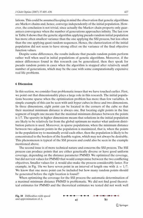
The second issue is of more technical nature and concerns the SSI process. The SSIprocess can produce points that are either genetically diverse or have good uniformcoverage, depending on the distance parameter PMMD. We optimized the coverage,but did not test values for PMMD that would compromise between the two conflictingobjectives. Smaller values for � would also make the process considerably faster. Forexample, in Fig. 10a we have seven point in an interval of length one with � = 1/7.We know that one more point can be included but how many random points shouldbe generated before the right location is found?

When optimizing the coverage for the SSI process the automatic determination ofa maximal minimum distance PMMD is problematic. We did not find good theoret-ical estimates for PMMD and the theoretical estimates we tested did not work well

Fig. 10 Difficulties with speedand approximation of � b)a)

428 J Glob Optim (2007) 37:405–436

in practice. Hence, we used experimental estimates. In our current implementation,we have numerically solved maximal values of PMMD for some number of pointsin some dimensions, and we approximate maximal PMMD elsewhere using interpo-lation. Examples of values used for � in our experiments for different numbers ofvariables (with population size 200) include 0.032 (for n = 2), 0.23 (for n = 5), 0.49(for n = 10), 0.64 (for n = 20), 0.79 (for n = 50) and 0.84 (for n = 100). Some furtherresearch is needed before the SSI process with maximal values for PMMD can beused in practical applications. An example of the difficulty of approximating the valueof � is given in Fig. 10b. Let us assume that we have fixed � = 1/7 and the distancebetween the end points of the interval and outermost points is 1/8 and the distancebetween intermediate points is 2/8. Here we have only four points (denoted by blackdots in the figure) and cannot fit any more points even though eight points could befit in the interval in the optimal case (denoted by circles in the figure). In other words,it is very hard to determine the maximal minimum distance a priori when points aregenerated randomly.

The third issue concerns the speed of point generators. We point out that the com-putational complexity of an algorithm may depend strongly on the implementation,see, e.g., [4], where bit-operations are considered. Thus, the results on the speed ofthe generators can be considered only suggestive.

The last issue concerns the testing of point generators. There exists a large varietyof dynamic statistical tests for the independence of points generated by point gener-ators [14]. These tests are called goodness-of-fit tests. One well-established batteryof goodness-to-fit tests is called DIEHARD and the source code is available at [8].However, the goodness-to-fit tests are designed to test the independence of largenumbers of points. For example, DIEHARD requires a binary file of a size 10–11megabytes to evaluate a generator. Since we are only interested in a few hundrednumbers at the beginning of the sequence, we used the Ripley’s K-function instead ofthe goodness-to-fit tests.

7 Conclusions and future research

In this paper, we have tested different initial populations for a real coded geneticalgorithm. Traditionally, pseudo random numbers are used for generating initial pop-ulation, and our motivation has been to study and initiate discussion on whether theiruse is justified.

We have shown with a simple, academic, example that initial populations may havea significant effect on the best objective function value over several generations. Thenwe have concentrated on studying different realistic ways to generate initial popu-lations for a case with no a priori information on the location of the global minima.We have briefly summarized the basic properties of a pseudo and a quasi randomsequence generator, the SSI process and the nonaligned systematic sampling andapplied them. We have discussed their properties including genetic diversity and agood uniform coverage for the points as well as speed and usability for the generators.In the numerical tests with genetic algorithms, we have used a test suite of 52 functionsfrom the literature. We have studied the effects of the different initial populations onthe best objective function values after 10 and 20 generations and after running thewhole algorithm.

J Glob Optim (2007) 37:405–436 429

There were differences in the coverage and genetic diversity of the tested pointsets. The SSI process has a good uniform coverage, but only average genetic diversity,and for pseudo random points it is vice versa. The Niederreiter quasi random pointshave both above average coverage and above average genetic diversity.

In the numerical experiments with the genetic algorithms, there was a trend—although weak—showing that the versions of genetic algorithm with good geneticdiversity converged fast during the first generations, but did not obtain the best finalobjective function values on the average. The converse was true for the versions withgood uniform coverage. However, the differences were not so large that any strongconclusion could be drawn.

With respect to the speed and usability of the point generators the results show thatpseudo and quasi random sequence generators are fast and easy to use. Both the SSIprocess and the nonaligned systematic sampling require more developing and testing.

We conclude that, based on our research, the traditional way to generate initialpopulations of genetic algorithms using pseudo random number generator was notworse than the others. It is particularly well suited to cases where the algorithm mustbe stopped prematurely; which may happen with computationally expensive reallife problems. However, there are also good alternative ways such as quasi randomsequences and the SSI process, which have advantages in certain cases, especiallyif the goodness of the final solution is valued higher that the speed of convergenceduring the first generations.

Our findings show that paying attention to the initial population may have aneffect on the success of the genetic algorithm and further research and discussionis encouraged. The topics for future research include, firstly, to study different ini-tial populations for specific types of problems and with different genetic algorithmparameters like population size and maximum number of generations. Secondly, tostudy more closely the problem of dimensionality discussed in Section 6, and thirdly,to further develop the SSI implementation and to discover good theoretical estimatesfor the maximal minimum distance PMMD.

Acknowledgements The authors thank doctors Salme Kärkkäinen and Marko M. Mäkelä for usefuldiscussions and professor Michael Mascagni for providing the Niederreiter generator. This researchwas supported by the Jenny and Antti Wihuri Foundation and the Academy of Finland, grant number102020.

Appendix A

This appendix is designed to give a short overview to different pseudo random numberand quasi random sequence generators. In the following definitions we use (y)modMto denote y modulo M.

A.1 Some pseudo random number generators

Traditionally, pseudo random number generators produce sequences of scalars. Ifvectors are needed, then they are usually formed by taking the first n scalars forthe first n-dimensional vector, the next n scalars for the second vector and so forth.According to [30], it would be preferable to generate pseudo random vectors directly.Here, we present traditional pseudo random number generators and one vectorgenerator.

430 J Glob Optim (2007) 37:405–436

We classify pseudo random number generators to two main categories: congruen-tial and recursive generators. We call a method congruential, if it uses modulo and onlythe previous iteration value, and we call it recursive, if it uses values from several previ-ous iterations. In addition, we present a feedback shift register generator and a vectorgenerator called SQRT-generator, which do not fall into the two main categories. Foranother classification, see, e.g., [39]. The classifications are always somewhat vague.Feedback shift register generator also uses values from several previous iterations,but its construction differs significantly from recursive generators, and therefore, weput it in its own class. For more detailed information about pseudo random numbergeneration we refer to [14] and to references therein.

A.1.1 Congruential generators

Next, we present five congruential generators. They are called linear, quadratic, inver-sive, additive and parallel linear congruential generators. The name congruentialcomes from the use of modulo. For example, in modulo 5, the numbers 4 and 9 arecalled congruent. In what follows, M is the modulo and aj’s are prescribed integers. Onthe ith iteration, the generators first produce an integer yi ∈ [0, M) and then a randomnumber xi ∈ [0, 1) is obtained by a division xi = yi/M unless another formula is given.The seed y0 is a large prescribed integer. An additive congruential generator (of kthorder) [45], to be described below, requires k + 1 seeds 0 ≤ y0

j < M, j = 0, . . . , k, andthe parallel linear generator includes three separate linear generators denoted by yi,yi and ˆyi.

Linear yi = (a1yi−1 + a2)mod M

Quadratic yi = (a1(yi−1)2 + a2yi−1 + a3)mod M

Inversive yi = (a1

(1

yi−1

)+ a2)mod M

Additive yi0 = yi−1

0yi

m = (yim−1 + yi−1

m )mod M, m = 1, ..., k

xi = yik

M

Parallel linear yi = (a1yi−1)mod M1yi = (a2yi−1)mod M2ˆyi = (a3

ˆyi−1)mod M3

xi = (yi

M1+ yi

M2+ ˆyi

M3)mod 1.

In all of the above generators i = 1, 2, . . . Often, a distinction is made between linearcongruential generators with a2=0 and a2 �=0. Then a generator with a2=0 is called amultiplicative linear congruential generator and a generator with a2 �=0 a mixed linearcongruential generator.

A.1.2 Recursive generators

Generators using two or more previous random numbers when generating a newnumber in the sequence are here called recursive generators. In what follows, aj, ci, s,

J Glob Optim (2007) 37:405–436 431

and r are prescribed integers s < r, j = 1, . . . , k, and ci is called the carry operator onthe ith iteration. The determination of ci is omitted for the multiply-with-carry-gener-ator and also for the add-with-carry and substract-with-borrow generators using morethat two previous values. Again, the pseudo random number xi ∈ [0, 1) is obtained bya division xi = yi/M. For more details about the carry operator, see, e.g., [6]. Next, wepresent five recursive generators.

Multiplicative recursive yi = (a1yi−1 + · · · + akyi−k)mod M

Lagged Fibonacci yi = (yi−r − yi−s)modM

Add − with − carry yi = (yi−s + yi−r + ci)mod M, where

ci ={

1, yi−s + yi−r + ci−1 ≤ M0, otherwise

Substract − with − borrow yi = (yi−s − yi−r − ci)mod M, where

ci ={

1, if yi−s − yi−r − ci < 00, otherwise

Multiply − with − carry yi = (a1yi−s + a2yi−r + ci)modM, where ci iscomputed using ci−1 and previous values of yi.

Again i = 1, 2, . . . and y0 is the seed. The number of previous values of y used in themethods described above may alter. In addition, the lagged Fibonacci generator maygenerate new values also as a sum or a product of the previous values.

A.1.3 Feedback shift register generator

Feedback shift register generator uses modulo in a different manner compared tothe congruential and recursive generators. Modulo M is not a large integer, but veryoften M = 2 in which case the generator produces a sequence

{αj

}of zeros and ones.

The sequence is then cut into subsequences with an appropriate length. These subse-quences correspond to yi’s. To generate the sequence

{αj

}, first a primitive polynomial

q(z) of order p is selected

q(z) = zp − (a1zp−1 + · · · + ap−1z + ap), (1)

where ai ∈ {0, 1, . . . , M − 1}, i = 1, . . . , p. Then using the coefficients ai, the nth num-ber in the sequence is generated using the formula

αn = (apαn−p + ap−1αn−p+1 + · · · + a1α

n−1)mod M. (2)

The initial numbers α1, . . . , αp ∈ [0, M) can be selected arbitrarily.

432 J Glob Optim (2007) 37:405–436

A.1.4 SQRT sequence

The following definition of the SQRT sequence is taken from [43]. Let pi now be theith prime number and zi = √

pi, i = 1, . . . , n. Then the n-dimensional SQRT sequence{xi} is defined by

xi = (iz) = (iz1, . . . , izn)mod 1,

where the modulo is taken component-wise. Despite its simplicity, the SQRT sequenceperforms well in [43], where it is applied to a numerical integration problem and com-pared with five quasi random sequences.

A.2 Some quasi random sequence generators

To describe the structure and the distribution properties of some quasi random se-quences let us define an elementary interval in base b

E =n∏

i=1

[ai

bdi,

ai + 1bdi

),

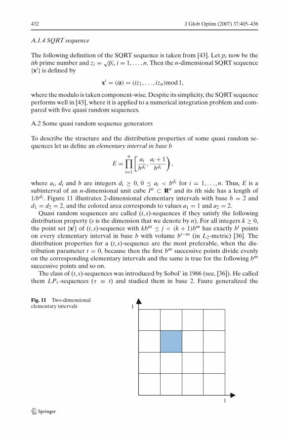
where ai, di and b are integers di ≥ 0, 0 ≤ ai < bdi for i = 1, . . . , n. Thus, E is asubinterval of an n-dimensional unit cube In ⊂ Rn and its ith side has a length of1/bdi . Figure 11 illustrates 2-dimensional elementary intervals with base b = 2 andd1 = d2 = 2, and the colored area corresponds to values a1 = 1 and a2 = 2.

Quasi random sequences are called (t, s)-sequences if they satisfy the followingdistribution property (s is the dimension that we denote by n). For all integers k ≥ 0,the point set {xj} of (t, s)-sequence with kbm ≤ j < (k + 1)bm has exactly bt pointson every elementary interval in base b with volume bt−m (in L2-metric) [36]. Thedistribution properties for a (t, s)-sequence are the most preferable, when the dis-tribution parameter t = 0, because then the first bm successive points divide evenlyon the corresponding elementary intervals and the same is true for the following bm

successive points and so on.The class of (t, s)-sequences was introduced by Sobol’ in 1966 (see, [36]). He called

them LPτ -sequences (τ ≡ t) and studied them in base 2. Faure generalized the

Fig. 11 Two-dimensionalelementary intervals 1

1

J Glob Optim (2007) 37:405–436 433

(t, s)-sequences to arbitrary prime base b ≥ 2 (see, e.g., [36]). Finally, Niederreitergeneralized (t, s)-sequence to arbitrary base b ≥ 2.

Often a (t, s)-sequence is called the Sobol’ sequence if b = 2 and t = 0, and Fauresequence if b is a prime and t = 0 [30]. Sequences that are constructed according to theguidelines given in [30] are called Niederreiter sequences. For a general constructionof any (t, s)-sequence, see, e.g., [20, 30].

Next, we present some examples how to construct (t, s)-sequences. We omit allimplementational details.

A.2.1 Van der Corput sequence

Let b ≥ 2 be the base and k be an integer. If we write k in base b

k = (dj...d1)b,

where di ∈ {0, . . . , b − 1}, i = 1, . . . , j, and define a radical inverse function φb by

φb(k) = d1

b+ · · · + dj

bj = (0.d1 . . . dj)b, (3)

then Van der Corput sequence in base b is the sequence {φb(k)}∞k=0. Informally, wemay say that in the radical inverse the numbers dj, . . . , d1 are reflected using the deci-mal point as a reflector, for example, if k = 12 = (1100)2, then φ2(12) = 0.00112. Vander Corput sequence is a 1-dimensional (t, s)-sequence with t = 0 (see, e.g., [30]).

A.2.2 Hammersley sequence

All but the first component of the n-dimensional Hammersley sequence are van derCorput sequences in an appropriate base. The n-dimensional Hammersley sequenceis defined as

xi = (i/N, φb1(i), . . . , φbn−1(i)), i = 0, 1, . . . , N − 1 (4)

where N is the number of points to be generated and the bases b1, . . . , bn are integersgreater than one and pairwise prime.

A.2.3 Halton sequence

A Hammersley sequence without the first element is called Halton sequence [17]

xi = (φb1(i), . . . , φbn(i)), i = 0, 1, . . . . (5)

The advantage over the Hammersley sequence is that a Halton sequence does notrequire the knowledge of N, the total length of the sequence.

A.2.4 Sobol’ sequence

We construct the Sobol’ sequence following [4] and [14]. Let us first consider1-dimensional Sobol’ sequence, for which we need to create a set of direction num-bers vi in base 2. To create the direction numbers vi, we use coefficients of a primitivepolynomial q in the field of binary numbers (compare to Eq. 1 in Sect. 7)

q(z) = zp + a1zp−1 + · · · + ap−1z + ap. (6)

434 J Glob Optim (2007) 37:405–436

Then, employing the bitwise binary exclusive-or operator ⊕ we derive the directionnumbers from the formula

vi = a1vi−1 ⊕ a2vi−2 ⊕ · · · ⊕ apvi−p ⊕ vi−p

2p , i > p.

The ith recurrence in 1-dimensional Sobol’ sequence is now formed as

xi = b1v1 ⊕ b2v2 ⊕ b3v3 ⊕ · · · ,

where · · · b3b2b1 is the binary representation of i (for example, if i = 1011, thenb4 = 1, b3 = 0, b2 = 1 and b1 = 1). To generate an n-dimensional sequence, it issufficient to choose n different primitive polynomials and calculate n different sets ofdirection numbers. For more details, see [4].

A.2.5 Faure sequence

The following example of Faure sequence is mainly from [43]. Let us define a function g

g(φb(k)) = c0

b+ · · · + cj−1

bj ,

where b is the base, φb(k) = (0.d1 . . . dj)b is an element of the Van der Corputsequence and

cm =

j∑

n=m

h!m(h − m)!dh

mod b.

Now, an n-dimensional (t, s)-sequence is defined as

xi = (φb(i), g(φb(i)), . . . , gn−1(φb(i))),

and a Faure sequence is obtained when b is the smallest prime larger or equal to thedimension n [36].

References

1. Acworth, P., Broadie, M., Glasserman, P.: A comparison of some Monte Carlo and quasi MonteCarlo techniques for option pricing. In: Niederreiter, H., Hellekalek, P., Larcher, G., Zinterhof,P. (eds). Monte Carlo and Quasi-Monte Carlo Methods 1996, number 127 in Lecture notes instatistics, pp. 1–18. Springer-Verlag, New York (1998)

2. Ali, M.M., Storey, C.: Modified controlled random search algorithms. Int. J. Comput. Mathemat.53, 229–235 (1994)

3. Ali, M.M., Storey, C.: Topographical multilevel single linkage. J. Global Optimizat. 5(4), 349–358(1994)

4. Bratley, P., Fox, B.L.: Algorithm 659: implementing Sobol’s quasirandom sequence generator.ACM Trans. Mathemat. Software 14(1), 88–100 (1988)

5. Bratley, P., Fox, B.L., Niederreiter, H.: Implementation and tests of low-discrepancy sequences.ACM Trans. Model. Comput. Simulat. 2(3), 195–213 (1992)

6. Couture, R., L’Ecuyer, P.: Distribution properties of multiply-with-carry random numbergenerators. Mathemat. Computat. 66(218), 591–607 (1997)

7. Dekkers, A., Aarts, E.: Global optimization and simulated annealing. Mathemat. Program. 50(3),367–393 (1991)

8. DIEHARD: a battery of tests for random number generators developed by George Marsaglia.http://stat.fsu.edu/~geo/diehard.html, September (2004).

9. Diggle, P.J.: Statistical Analysis of Spatial Point Patterns. Academic Press, London (1983)

J Glob Optim (2007) 37:405–436 435

10. Dykes, S., Rosen, B.: Parallel very fast simulated reannealing by temperature block partitioning.In Proceedings of the 1994 IEEE International Conference on Systems, Man, and Cybernetics,vol. 2, pp. 1914–1919 (1994)

11. Eiben, A.E., Hinterding, R., Michalewicz, Z.: Parameter control in evolutionary algorithms. IEEETrans. Evol. Computat. 3(2), 124–141 (1999)

12. Floudas, C.A., Pardalos, P.M. (eds.): Recent Advances in Global Optimization. Princeton Univer-sity Press, Princeton, NJ (1992)

13. Genetic and evolutionary algorithm toolbox for use with Matlab. http://www.geatbx.com/, June(2004)

14. Gentle, J.E.: Random Number Generation and Monte Carlo Methods. Springer-Verlag, New York(1998)

15. Glover, F., Kochenberger, G.A. (eds.): Handbook of Metaheuristics. Kluwer Academic Publishers,Boston (2003)

16. Goldberg, D.E.: Genetic Algorithms in Search, Optimization, and Machine Learning. Addison-Wesley, New York (1989)

17. Halton, J.H.: On the efficiency of certain quasi-random sequences of points in evaluating multi-dimentional integrals. Numerische Mathematik, 2, 84–90 (1960)

18. Horst, R., Pardalos, P.M. (eds.): Handbook of Global Optimization. Kluwer Academic Publishers,Dordrecht (1995)

19. Kingsley, M.C.S., Kanneworff, P., Carlsson, D.M.: Buffered random sampling: a sequential inhib-ited spatial point process applied to sampling in a trawl survey for northern shrimp pandalusborealis in west Greenland waters. ICES J. Mar. Sci. 61(1), 12–24 (2004)

20. Larcher, G.: Digital point sets: analysis and applications. In: Hellekalek, P., Larcher, G. (eds.)Random and Quasi Random Point Sets, number 138 in Lecture Notes in Statistics, pp. 167–222.Springer-Verlag, New York (1998)

21. Lei, G.: Adaptive random search in quasi-Monte Carlo methods for global optimization. Comput.Mathemat. Appl. 43(6–7), 747–754 (2002)

22. Lemieux, C., L’Ecuyer, P.: On selection criteria for lattice rules and other quasi-Monte Carlo pointsets. Mathemat. Comput. Simulat. 55(1–3), 139–148 (2001)

23. Maaranen, H.: On Global Optimization with Aspects to Method Comparison and Hybridization.Licentiate thesis, Department of Mathematical Information Technology, University of Jyväskylä(2002)

24. Maaranen, H., Miettinen, K., Mäkelä, M.M.: Quasi-random initial population for genetic algo-rithms. Comput. Mathemat. Appl. 47(12), 1885–1895 (2004)

25. Michalewicz, Z.: Genetic Algorithms + Data Structures = Evolution Programs. Springer-Verlag,Berlin (1994)

26. Michalewicz, Z., Logan, T.D., Swaminathan, S.: Evolutionary operators for continuous convexparameter spaces. In: Sebald, A.V., Fogel, L.J. (eds.) Proceedings of the 3rd Annual Conferenceon Evolutionary Programming, pp. 84–97. World Scientific Publishing, River Edge, NJ (1994)

27. Morokoff, W.J., Caflisch, R.E.: Quasi-random sequences and their discrepancies. SIAM J. Sci.Comput. 15(6), 1251–1279 (1994)

28. Neter, J., Wasserman, W., Whitmore, G.A.: Applied Statistics. Allyn and Bacon, Inc., Boston, thirdedition (1988)

29. Niederreiter, H.: Quasi-Monte Carlo methods for global optimization. In: Grossmann, W., Pflug,G., Vincze, I., Wertz, W. (eds.) Proceedings of the 4th Pannonian Symposium on MathematicalStatistics, pp. 251–267 (1983)

30. Niederreiter, H.: Random Number Generation and Quasi-Monte Carlo Methods. SIAM, Phila-delphia (1992)

31. Nix, A.E., Vose, M.D.: Modeling genetic algorithms with Markov chains. Ann. Mathemat. Arti.Intell. 5(1), 79–88 (1992)

32. Pardalos, P.M., Romeijn, H.E. (eds.): Handbook of Global Optimization, vol. 2. Kluwer AcademicPublishers, Boston (2002)

33. Press, W.H., Teukolsky, S.A.: Quasi- (that is, sub-) random numbers. Comput. Phys. 3(6), 76–79(1989)

34. Ripley, B.D.: Spatial Statistics. John Wiley & Sons, New York (1981)35. Snyder, W.C.: Accuracy estimation for quasi-Monte Carlo simulations. Mathemat Comput. Sim-

ulat. 54(1–3), 131–143 (2000)36. Sobol’, I.M.: On quasi-Monte Carlo integrations. Mathemat. Comput. Simulat. 47(2–5), 103–112

(1998)37. Sobol’, I.M., Bakin, S.G.: On the crude multidimensional search. J. Computat. Appl. Mathemat.

56(3), 283–293 (1994)

436 J Glob Optim (2007) 37:405–436

38. Sobol, I.M., Tutunnikov, A.V.: A varience reducing multiplier for Monte Carlo integrations. Math-emat. Comput. Model. 23(8–9), 87–96 (1996)

39. Tang, H.-C.: Using an adaptive genetic algorithm with reversals to find good second-order multiplerecursive random number generators. Mathemat. Methods Operat. Res. 57(1), 41–48 (2003)

40. Test problems for global optimization. http://www.imm.dtu.dk/~km/GlobOpt/testex/, June (2004)41. Test problems in R2. http://iridia.ulb.ac.be/~aroli/ICEO/Functions/Functions.html, June (2004)42. Trafalis, B., Kasap, S.: A novel metaheuristics approach for continuous global optimization.

J. Global Optimizat. 23(2), 171–190 (2002)43. Tuffin, B.: On the use of low discrepancy sequences in Monte Carlo methods. Monte Carlo Meth-

ods Appl. 2(4), 295–320 (1996)44. Weisstein, E.W.: “circle packing”. From MathWorld–A Wolfram Web Resource. http://math-

world.wolfram.com/CirclePacking.html, September (2004)45. Wikramaratna, R.S.: ACORN—a new method for generating sequences of uniformly distributed

pseudo-random numbers. J. Computat. Phys. 83(1), 16–31 (1989)46. Wright, A.H., Zhao, Y.: Markov chain models of genetic algorithms. In: Banzhaf, W., Daida, J.,

Eiben, A.E., Garzon, M.H., Honavar, V., Jakiela, M., Smith, R.E. (eds.) GECCO-99: Proceed-ings of the Genetic and Evolutionary Computation Conference, pp. 734–741. Morgan Kauffman,SanMateo, California (1999)