1

Other Still Image Compression Standards

Tzu-Heng Henry Lee, Po-Hong Wu

Introduction

Today, there are many compression standards that have been developed by

companies or researchers. In this tutorial, we introduce some compression standards

that are popular in the recent years. All these compression standards have its own

advantages and disadvantages and we will give an overview in the following articles.

First, we will introduced the JPEG 2000 (Joint Photographic Experts Group 2000)

compression standard followed by the JPEG-LS (Joint Photographic Experts Group –

Lossless Standard), the JBIG2 (Joint Bi-level Image Experts Group), the GIF

(Graphics Interchange Format), the LZ77 (Lempel-Ziv 77), the PNG (Portable

Network Graphics), HD photo, and the TIFF (Tag Image File Format) in order.

However, some compressions involve difficult algorithms that are too difficult to be

introduced appropriately here. We only introduce the main idea of each compression

without mathematical details.

2

CONTENTS

Chapter 1 JPEG 2000 ................................................................................................ 4

1.1 Fundamental Building Blocks ........................................................................ 4

1.2 Wavelet Transform ......................................................................................... 6

Chapter 2 JPEG-LS................................................................................................... 9

2.1 Modeler .......................................................................................................... 9

2.2 Coding .......................................................................................................... 12

Chapter 3 JBIG2 ...................................................................................................... 13

3.1 Text Image Data ........................................................................................... 13

3.2 Halftones ...................................................................................................... 15

3.3 Arithmetic Entropy Coding .......................................................................... 16

Chapter 4 GIF .......................................................................................................... 17

4.1 LZW Data Compression .............................................................................. 17

4.2 Implementation Challenges of LZW Algorithm .......................................... 21

4.3 Application of LZW Algorithm in Image Compression .............................. 22

Chapter 5 PNG......................................................................................................... 24

5.1 Huffman Coding in the Deflate Format ....................................................... 25

5.2 LZ77-Related Compression Algorithm Details ........................................... 27

Chapter 6 HD Photo (JPEG XR) ........................................................................... 29

6.1 Data Hierarchy ............................................................................................. 29

6.2 HD Photo Compression Algorithm .............................................................. 32

Chapter 7 TIFF 6.0 .................................................................................................. 33

7.1 Difference Predictor ..................................................................................... 33

7.2 PackBits Compression ................................................................................. 33

3

7.3 Modified Huffman Compression ................................................................. 35

Chapter 8 Conclusion and Comparison ................................................................ 36

REFERENCES .............................................................................................................. 38

4

Chapter 1 JPEG 2000

Equation Chapter (Next) Section 1

The JPEG 2000 (Joint Photographic Experts Group 2000) compression standard

employs the wavelet transform as its core transform algorithm [1], [5], [6]. This

standard is developed to overcome the shortcomings of the baseline JPEG. Instead of

using the low-complexity and memory efficient block discrete cosine transform (DCT)

that was used in the JPEG standard, the JPEG 2000 uses the discrete wavelet

transform (DWT) that is based on multi-resolution image representation [7]. The main

purpose of the wavelet analysis is to obtain different approximations of a function f(x)

at different levels of resolution [1], [4]. Both the mother wavelet ( )x and the

scaling function ( )x are important functions to be considered in multiresolution

analysis [4]. The DWT also improves compression efficiency due to good energy

compaction and the ability to decorrelate the image across a larger scale. The

JPEG2000 has also replaced the Huffman coder of the baseline JPEG with a

context-based adaptive binary arithmetic coder known as the MQ coder [6].

1.1 Fundamental Building Blocks

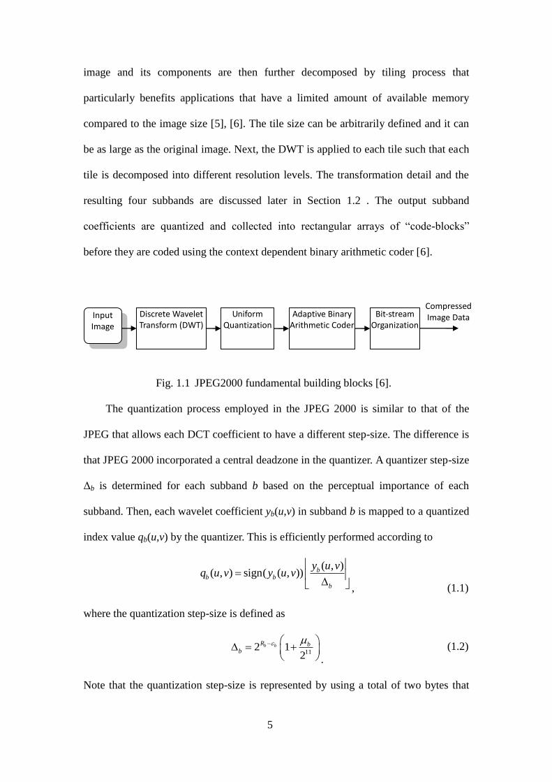
The fundamental building block of JPEG2000 is illustrated in Fig. 1.1. Similar to

the JPEG, a core transform coding algorithm is first applied to the input image data.

After quantizing and entropy coding the transformed coefficients, the output

codestream or the so-called bitstream are formed. Each of the blocks will be described

in more detail.

Before the image data is fed into the transform block, the source image is

decomposed into three color components, either in RGB or YCbCr format. The input

5

image and its components are then further decomposed by tiling process that

particularly benefits applications that have a limited amount of available memory

compared to the image size [5], [6]. The tile size can be arbitrarily defined and it can

be as large as the original image. Next, the DWT is applied to each tile such that each

tile is decomposed into different resolution levels. The transformation detail and the

resulting four subbands are discussed later in Section 1.2 . The output subband

coefficients are quantized and collected into rectangular arrays of “code-blocks”

before they are coded using the context dependent binary arithmetic coder [6].

Fig. 1.1 JPEG2000 fundamental building blocks [6].

The quantization process employed in the JPEG 2000 is similar to that of the

JPEG that allows each DCT coefficient to have a different step-size. The difference is

that JPEG 2000 incorporated a central deadzone in the quantizer. A quantizer step-size

Δb is determined for each subband b based on the perceptual importance of each

subband. Then, each wavelet coefficient yb(u,v) in subband b is mapped to a quantized

index value qb(u,v) by the quantizer. This is efficiently performed according to

( , )( , ) sign( ( , )) b

b b

b

y u vq u v y u v

, (1.1)

where the quantization step-size is defined as

11

2 12

b bR bb

.

(1.2)

Note that the quantization step-size is represented by using a total of two bytes that

Input Image

Discrete Wavelet Transform (DWT)

Adaptive Binary Arithmetic Coder

Uniform Quantization

Bit-stream Organization

Compressed Image Data

6

contains an 11-bit mantissa μb and a 5-bit exponent εb. The dynamic range Rb depends

on the number of bits used to represent the original image tile component and on the

choice of the wavelet transform [6]. For reversible operation, the quantization step

size is required to be 1 (when μb = 0 and εb = Rb).

The implementation of the MQ-coder is beyond the scope of this research and for

further reading on this subject, the coding details of the MQ-coder are discussed in

[8].

1.2 Wavelet Transform

A two-dimensional scaling function, ( , )x y , and three two-dimensional

wavelets ( , )H x y , ( , )V x y and ( , )D x y are critical elements for wavelet

transforms in two dimensional case [1]. The scaling function and the directional

wavelets are composed of the product of a one-dimensional scaling function and the

corresponding wavelet which are demonstrated as the following:

( , ) ( ) ( )x y x y (1.3)

( , ) ( ) ( )H x y x y (1.4)

( , ) ( ) ( )V x y y x (1.5)

( , ) ( ) ( )D x y x y (1.6)

, where H measures the horizontal variations (horizontal edges), V corresponds

to the vertical variations (vertical edges), and D detects the variations along the

diagonal directions.

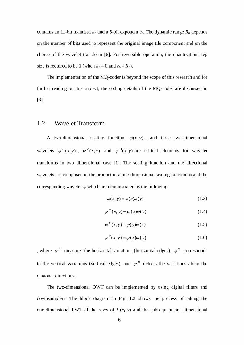
The two-dimensional DWT can be implemented by using digital filters and

downsamplers. The block diagram in Fig. 1.2 shows the process of taking the

one-dimensional FWT of the rows of f (x, y) and the subsequent one-dimensional

7

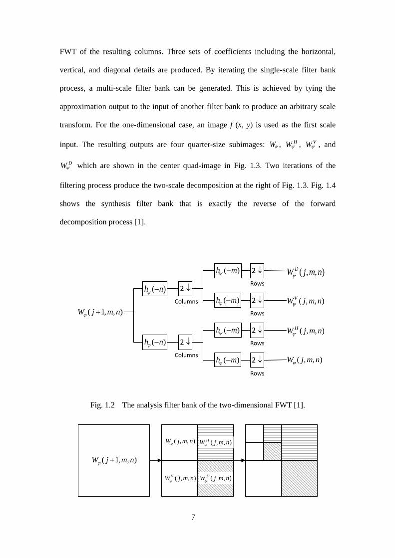
FWT of the resulting columns. Three sets of coefficients including the horizontal,

vertical, and diagonal details are produced. By iterating the single-scale filter bank

process, a multi-scale filter bank can be generated. This is achieved by tying the

approximation output to the input of another filter bank to produce an arbitrary scale

transform. For the one-dimensional case, an image f (x, y) is used as the first scale

input. The resulting outputs are four quarter-size subimages: W , HW , VW , and

DW which are shown in the center quad-image in Fig. 1.3. Two iterations of the

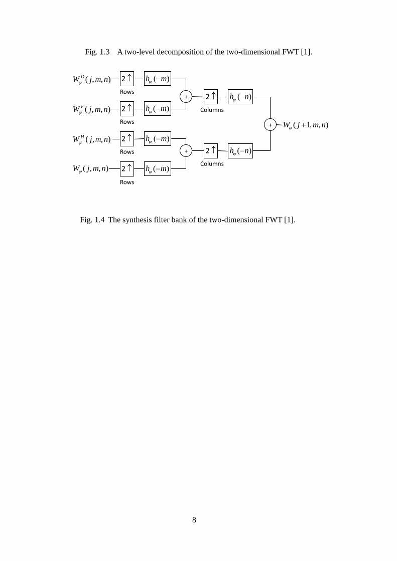
filtering process produce the two-scale decomposition at the right of Fig. 1.3. Fig. 1.4

shows the synthesis filter bank that is exactly the reverse of the forward

decomposition process [1].

Fig. 1.2 The analysis filter bank of the two-dimensional FWT [1].

( 1, , )W j m n

( , , )W j m n ( , , )HW j m n

( , , )VW j m n ( , , )DW j m n

( )h n

( 1, , )W j m n

( )h n

2

2

( , , )DW j m n

( , , )W j m n

( )h m 2

( )h m 2

( )h m 2

( )h m 2

( , , )VW j m n

( , , )HW j m n

Columns

Columns

Rows

Rows

Rows

Rows

8

Fig. 1.3 A two-level decomposition of the two-dimensional FWT [1].

Fig. 1.4 The synthesis filter bank of the two-dimensional FWT [1].

( )h n

( 1, , )W j m n

( )h n

2

2

( , , )DW j m n

( , , )W j m n

( )h m 2

( )h m 2

( )h m 2

( )h m 2

( , , )VW j m n

( , , )HW j m n

Columns

Columns

Rows

Rows

Rows

Rows

+

+

+

9

Chapter 2 JPEG-LS

Equation Chapter (Next) Section 1

The JPEG-LS (Joint Photographic Experts Group – Lossless Standard) [9], [10],

[11] is a near-lossless compression standard that was developed because at the time,

the Huffman coding based JPEG lossless standard and other standards are limited in

their compression performance. JPEG-LS, on the other hand, can obtain good

de-correlation. It is a simple and efficient baseline algorithm that consists of two

independent and distinct stages called modeling and encoding [10], [11]. Prior to

encoding, there are two essential steps to be done in the modeling stage:

de-correlation (prediction) and error modeling [9]. The core algorithm of the

JPEG-LS is called LOCO-I (LOw COmplexity LOssless COmpression for Images)

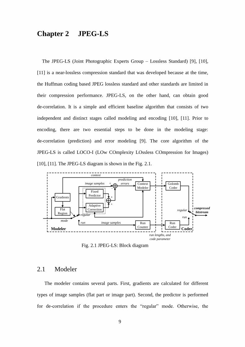
[10], [11]. The JPEG-LS diagram is shown in the Fig. 2.1.

Flat

Region

Gradients

Adaptive

Correction

Fixed

Predictor

Context

Modeler

Golomb

Coder

Run

Counter

Run

Coder

context

image samples

prediction

errors

run lengths, and

code parameter

regular

run

image samples

regular

runmode

compressed

bitstream

Modeler Coder

+

-

+

+

Fig. 2.1 JPEG-LS: Block diagram

2.1 Modeler

The modeler contains several parts. First, gradients are calculated for different

types of image samples (flat part or image part). Second, the predictor is performed

for de-correlation if the procedure enters the “regular” mode. Otherwise, the

10

procedure enters the “run” mode for more efficient coding. Finally, the predictor is

followed by the context modeler that is used for adaptive prediction.

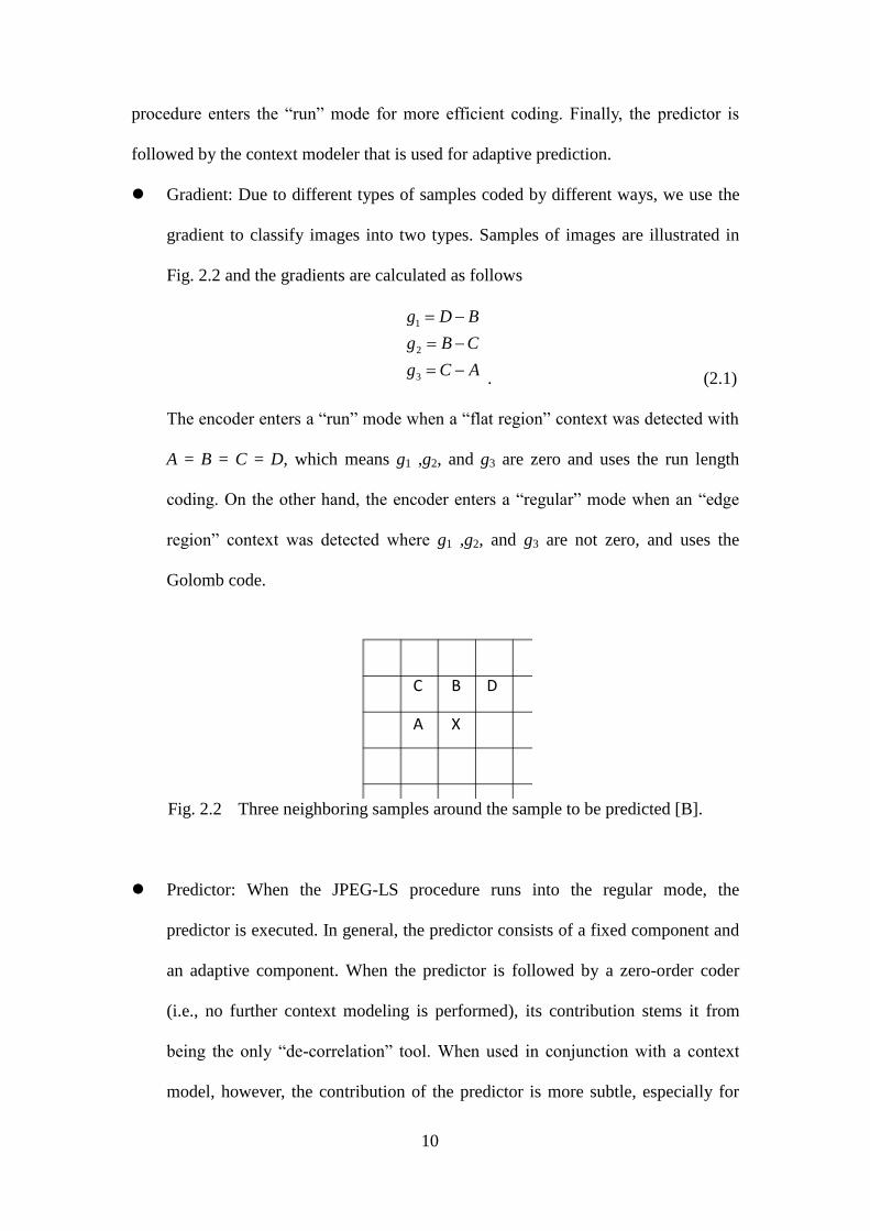
Gradient: Due to different types of samples coded by different ways, we use the

gradient to classify images into two types. Samples of images are illustrated in

Fig. 2.2 and the gradients are calculated as follows

1

2

3

g D B

g B C

g C A

. (2.1)

The encoder enters a “run” mode when a “flat region” context was detected with

A = B = C = D, which means g1 ,g2, and g3 are zero and uses the run length

coding. On the other hand, the encoder enters a “regular” mode when an “edge

region” context was detected where g1 ,g2, and g3 are not zero, and uses the

Golomb code.

Fig. 2.2 Three neighboring samples around the sample to be predicted [B].

Predictor: When the JPEG-LS procedure runs into the regular mode, the

predictor is executed. In general, the predictor consists of a fixed component and

an adaptive component. When the predictor is followed by a zero-order coder

(i.e., no further context modeling is performed), its contribution stems it from

being the only “de-correlation” tool. When used in conjunction with a context

model, however, the contribution of the predictor is more subtle, especially for

C

A

B

X

D

11

its adaptive component. In fact, the prediction may seem redundant at first, since

the same contextual information that is used to predict is also available for

building the coding model that will eventually learn the “predictable” patterns of

the data and assign probabilities accordingly. In the LOCO-I algorithm, primitive

edge detection of horizontal or vertical edges by examining the neighboring

pixels of the current pixel X as illustrated in Fig. 2.2. The pixel labeled by B is

used in the case of a vertical edge while the pixel located at A is used in the case

of a horizontal edge. This simple predictor is called the Median Edge Detection

(MED) predictor [9] or the LOCO-I predictor [10], [11]. The pixel X is predicted

by the LOCO-I predictor according to the following rules:

min( , ) max( , )

max( , ) min( , )

.

A B if C A B

X A B if C A B

A B C otherwise

.

(2.2)

The three simple predictors are selected according to the following conditions: (1)

It tends to choose B in cases where a vertical edge exists in the left of the X. (2)

It tends to choose A when there is a horizontal edge is above X. (3) It tends to

choose A + B – C if no edge is detected [11].

Context Model: Context model is a very simple and is determined by quantized

gradients. It is aimed at approaching the capability of the more complicated

universal context modeling techniques for capturing high-order dependencies.

The desired small number of free statistical parameters is achieved by adopting a

TSGD model that yields two free parameters per context. Reducing the number

of parameters is the key objective in the context modeling scheme for the

JPEG-LS.

12

2.2 Coding

Golomb codes: The data with a geometric distribution will have the Golomb

code as an optimal prefix code. It makes Golomb codes highly suitable for the

situations in which the occurrence of small values in the input stream is

significantly more likely than large values. The Rice coding denotes using a

subset of the family of Golomb codes to produce a simpler prefix code. Whereas

Golomb codes have a tunable parameter that can be any positive value, Rice

codes are in which the tunable parameter is a power of two. This makes Rice

codes convenient for use on a computer, since multiplication and division by 2

can be implemented more efficiently.

Run length codes: Golomb Rice codes are quite inefficient for encoding low

entropy distributions due to the fact that the coding rate is at least one bit per

symbol. Significant redundancy may be produced because the smooth regions in

an image can be encoded at less than 1 bit per symbol [9], [10], [11]. The

significantly excess code length over the entropy of context of the smooth

regions leads to undesired degradation in performance. To avoid having excess

code length over the entropy, alphabet extension is used by taking codes blocks

of symbols instead of coding individual symbols. This spreads out the excess

coding length over many symbols [9]. This is the “run” mode of the JPEG-LS

and it is executed once a flat or smooth context region characterized by zero

gradients is detected [11]. A run of west symbol “a” is expected and the end of

run occurs when a new symbol occurs or the end of line is reached. The total run

length is encoded and the encoder would return to the “regular” mode [9], [11].

13

Chapter 3 JBIG2

Equation Chapter (Next) Section 1

The JBIG2 (Joint Bi-level Image Experts Group) [12], [13] is a coding standard

developed by the Joint Bi-level Image Experts Group. It particularly deals with the

lossy and lossless compression of bi-level images such as scanned images or

facsimiles. The JBIG2 is able to achieve a good compression ratio and code lossy

images while preserving visually lossless quality for textual images. The JBIG2 also

allows both quality-progressive coding through refinement stages, with the

progression going from lower to higher (or lossless) quality, and content-progressive

coding, successively adding different types of image data (for example, first text, then

halftone). It will have a control structure that allows efficient encoding of multipage

documents in sequential or random-access mode, or embedded in another file format.

Typically, a bi-level image consists mainly of a large amount of textual and halftone

data in which the same shapes appear repeatedly and the bi-level image is segmented

into three regions: text, halftone, and generic regions. Each region is coded differently

and the coding methodologies are described in the following passage.

3.1 Text Image Data

Text coding is based on the nature of human visual interpretation. A human

observer cannot tell the difference of two instances of the same characters in a bi-level

image even though they may not exactly match pixel by pixel. Therefore, only the

bitmap of one representative character instance needs to be coded instead of coding

the bitmaps of each occurrence of the same character individually. For each character

instance, the coded instance of the character is then stored into a “dictionary” [12].

14

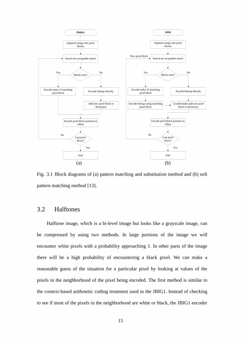
There are two encoding methods for text image data: pattern matching and

substitution (PM&S) and soft pattern matching (SPM). These methods are presented

in the following subsections [13].

1) Pattern matching and substitution: Due to different contents coded in different

ways, we segment of the image into pixel blocks, and search for a match in the

dictionary. If a match exists, we code an index of the corresponding

representative bitmap in the dictionary and the position of the character on the

page. The position is usually relative to another previously coded character [12].

If a match is not found, the segmented pixel block is coded directly and added

into the dictionary [13]. Typical procedures of pattern matching and substitution

algorithm are displayed in Fig. 3.1 (a). Although the method of PM&S can

achieve outstanding compression, substitution errors could be made during the

process if the image resolution is low [12].

2) Soft pattern matching: In addition to a pointer to the dictionary and position

information of the character as in PM&S, we include refinement coding that can

be used to recreate the original character on the page, yielding lossless

compression. The refinement coding is that the image or character will be

re-encoded using a two-plane bitmap coder, making use of previously coded

information in both the current image and the previously coded lossy image.

Since it is known that the current character is highly correlated with the matched

character, the prediction of the current pixel is more accurate [12], [13]. The only

difference between PM&S and SPM is that lossy direct substitution of the

matched character is replaced by a lossless encoding that uses the matched

character in the coding context. Unlike PM&S, lossy SPM does not need a very

safe and intelligent matching procedure to avoid substitution errors.

15

PM&S

Segment image into pixel

blocks

Search for acceptable match

Match exist?

Encode bitmap directlyEncode index of matching

pixel block

Add new pixel block to

dictionary

Encode pixel block position as

offset

Last pixel

block?

Yes No

End

Yes

No

SPM

Segment image into pixel

blocks

Search for acceptable match

Match exist?

Encode bitmap directlyEncode index of matching

pixel block

Conditionally add new pixel

block to dictionary

Encode pixel block position as

offset

Last pixel

block?

Yes No

End

Yes

No

Encode bitmap using matching

pixel block

Next pixel block

(a) (b)

Fig. 3.1 Block diagrams of (a) pattern matching and substitution method and (b) soft

pattern matching method [13].

3.2 Halftones

Halftone image, which is a bi-level image but looks like a grayscale image, can

be compressed by using two methods. In large portions of the image we will

encounter white pixels with a probability approaching 1. In other parts of the image

there will be a high probability of encountering a black pixel. We can make a

reasonable guess of the situation for a particular pixel by looking at values of the

pixels in the neighborhood of the pixel being encoded. The first method is similar to

the context-based arithmetic coding treatment used in the JBIG1. Instead of checking

to see if most of the pixels in the neighborhood are white or black, the JBIG1 encoder

16

uses the pattern of pixels in the neighborhood, or context to decide which set of

probabilities to use in encoding a particular pixel. In the second method, descreening

is performed on the halftone image so that the image is converted back to grayscale.

In this method, the bi-level image may be divided into pixel blocks, and the grayscale

values in the corresponding block may be the sum of the binary pixel values. The

converted grayscale values are then used as indexes of fixed-sized tiny bitmap

patterns contained in a halftone bitmap dictionary. This allows decoder to successfully

render a halftone image by presenting indexed dictionary bitmap patterns neighboring

with each other [12], [13].

3.3 Arithmetic Entropy Coding

All three region types including text, halftone, and generic regions may all use

arithmetic coding. JBIG2 specifically uses the MQ coder.

17

Chapter 4 GIF

Equation Chapter (Next) Section 1

The GIF (Graphics Interchange Format) is an image compression standard

aiming to transmit and interchange graphic data so that the format is independent of

the hardware used to display the data. The Graphics Interchange Format is divided

into blocks and sub-blocks and each of them contains relevant data information that

can be used to recreate a graphic image. The GIF format uses the

Variable-Length-Code LZW (Lempel-Ziv-Welch) Compression that is based on the

LZW compression. The following subsection provides an introduction on the LZW

algorithm [I].

4.1 LZW Data Compression

The Lempel Ziv approach is a simple algorithm that replaces string of characters

with single codes and adds new string of characters to a “string table” without doing

any analysis of the incoming text. When using 8-bit characters, by default, the first

256 codes are assigned to the standard character set and as the algorithm proceeds, the

rest codes are assigned to strings. For instance of 12 bit codes, the codes from 0 to 255

are individual bytes and codes 256 to 4095 are assigned to substrings [14].

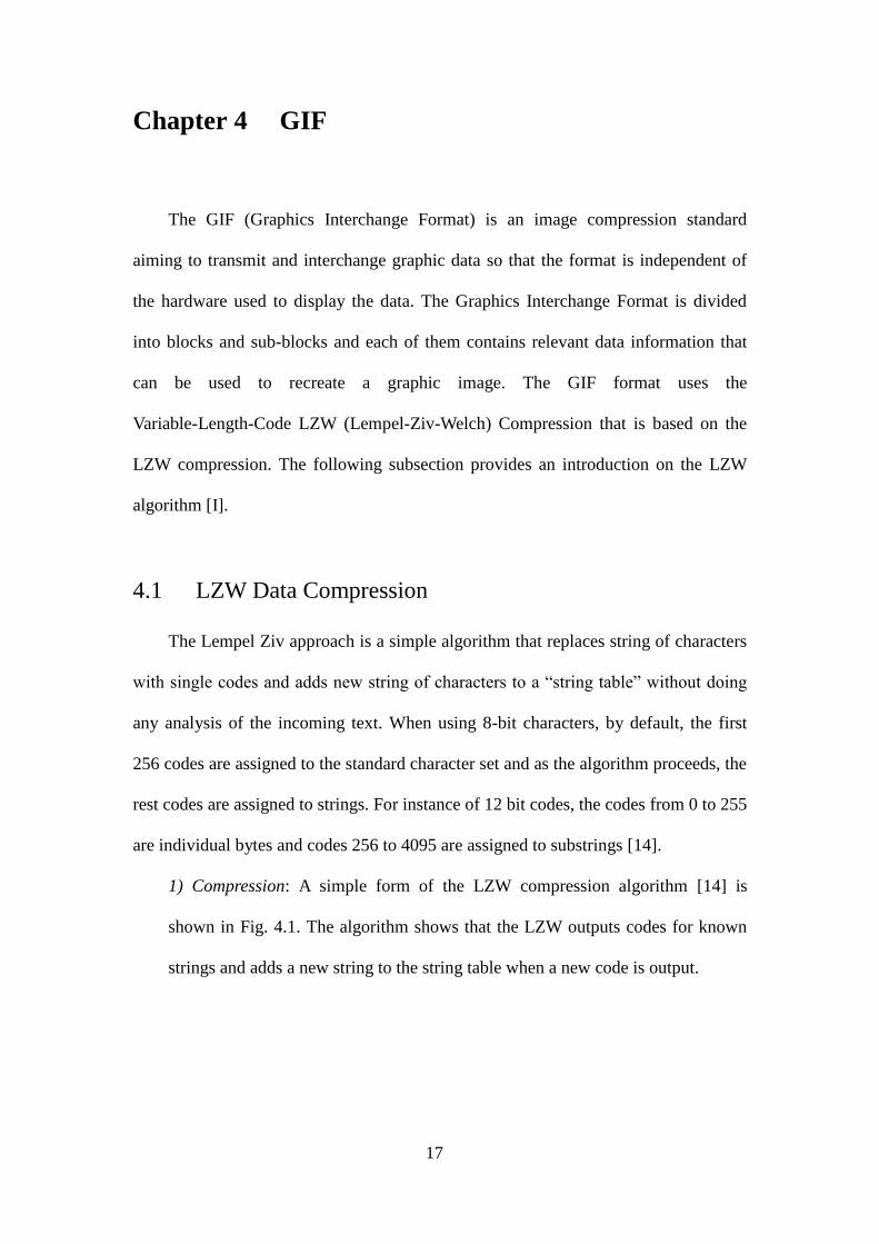
1) Compression: A simple form of the LZW compression algorithm [14] is

shown in Fig. 4.1. The algorithm shows that the LZW outputs codes for known

strings and adds a new string to the string table when a new code is output.

18

Fig. 4.1 The LZW compression algorithm [14].

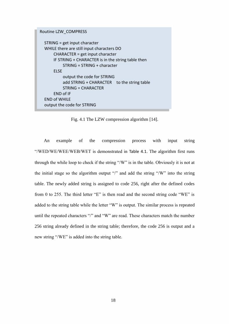
An example of the compression process with input string

“/WED/WE/WEE/WEB/WET is demonstrated in Table 4.1. The algorithm first runs

through the while loop to check if the string “/W” is in the table. Obviously it is not at

the initial stage so the algorithm output “/” and add the string “/W” into the string

table. The newly added string is assigned to code 256, right after the defined codes

from 0 to 255. The third letter “E” is then read and the second string code “WE” is

added to the string table while the letter “W” is output. The similar process is repeated

until the repeated characters “/” and “W” are read. These characters match the number

256 string already defined in the string table; therefore, the code 256 is output and a

new string “/WE” is added into the string table.

Routine LZW_COMPRESS

STRING = get input character WHILE there are still input characters DO CHARACTER = get input character IF STRING + CHARACTER is in the string table then STRING = STRING + character ELSE output the code for STRING add STRING + CHARACTER to the string table STRING = CHARACTER END of IF END of WHILE output the code for STRING

19

Table 4.1 An example of the LZW compression process [14].

Input String = /WED/WE/WEE/WEB/WET

Character Input Code Output New Code Value New String

/W / 256 /W

E W 257 WE

D E 258 ED

/ D 259 D/

WE 256 260 /WE

/ E 261 E/

WEE 260 262 /WEE

/W 261 263 E/W

EB 257 264 WEB

/ B 265 B/

WET 260 266 /WET

EOF T

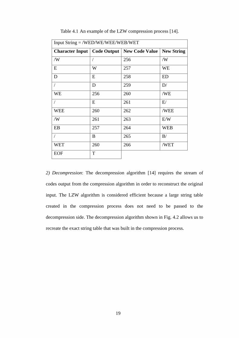
2) Decompression: The decompression algorithm [14] requires the stream of

codes output from the compression algorithm in order to reconstruct the original

input. The LZW algorithm is considered efficient because a large string table

created in the compression process does not need to be passed to the

decompression side. The decompression algorithm shown in Fig. 4.2 allows us to

recreate the exact string table that was built in the compression process.

20

Fig. 4.2 The LZW decompression algorithm [14].

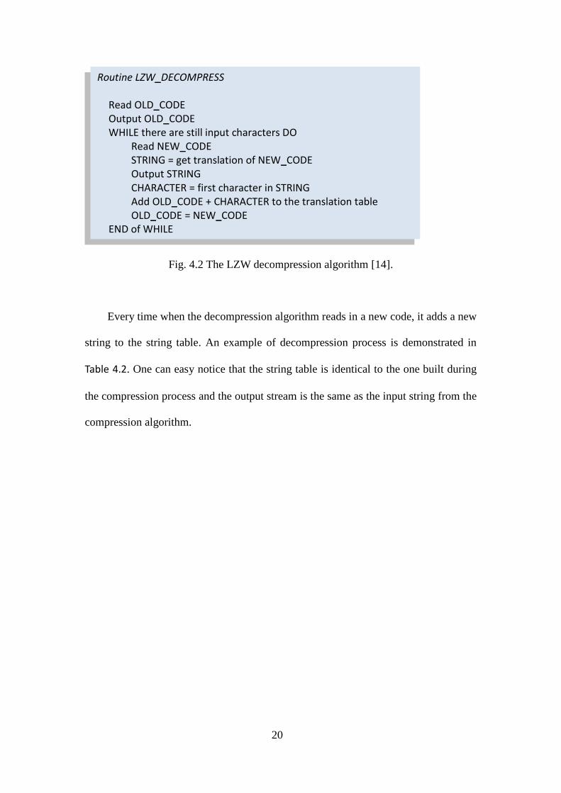
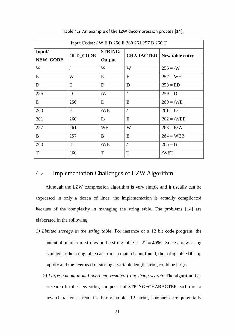
Every time when the decompression algorithm reads in a new code, it adds a new

string to the string table. An example of decompression process is demonstrated in

Table 4.2. One can easy notice that the string table is identical to the one built during

the compression process and the output stream is the same as the input string from the

compression algorithm.

Routine LZW_DECOMPRESS

Read OLD_CODE Output OLD_CODE WHILE there are still input characters DO Read NEW_CODE STRING = get translation of NEW_CODE Output STRING CHARACTER = first character in STRING Add OLD_CODE + CHARACTER to the translation table OLD_CODE = NEW_CODE END of WHILE

21

Table 4.2 An example of the LZW decompression process [14].

Input Codes: / W E D 256 E 260 261 257 B 260 T

Input/

NEW_CODE OLD_CODE

STRING/

Output CHARACTER New table entry

W / W W 256 = /W

E W E E 257 = WE

D E D D 258 = ED

256 D /W / 259 = D

E 256 E E 260 = /WE

260 E /WE / 261 = E/

261 260 E/ E 262 = /WEE

257 261 WE W 263 = E/W

B 257 B B 264 = WEB

260 B /WE / 265 = B

T 260 T T /WET

4.2 Implementation Challenges of LZW Algorithm

Although the LZW compression algorithm is very simple and it usually can be

expressed in only a dozen of lines, the implementation is actually complicated

because of the complexity in managing the string table. The problems [14] are

elaborated in the following:

1) Limited storage in the string table: For instance of a 12 bit code program, the

potential number of strings in the string table is 122 4096 . Since a new string

is added to the string table each time a match is not found, the string table fills up

rapidly and the overhead of storing a variable length string could be large.

2) Large computational overhead resulted from string search: The algorithm has

to search for the new string composed of STRING+CHARACTER each time a

new character is read in. For example, 12 string compares are potentially

22

required when we are using a code size of 12 bits. Generally, the computational

complexity for each string search take on the order of log2 string compares. This

computational overhead increases the string comparison time.

The amount of storage required depends on the total length of all the strings. The

storage problem can be solved by storing each string as a combination of a code and a

character. For the instance of the compression process shown in Table, the string

“/WEE” can be stored as code 260 with appended character “E”. The byte required in

the storage can be reduced from 5 bytes to 3 bytes. This method can also reduce the

amount of time for a string comparison. The method, however, cannot reduce the

number of comparisons that have to be made to find a match. A hashing algorithm can

be employed to solve this problem. We basically store a code in a location in the array

based on an address formed by the string itself instead of storing the code N in

location N of the array. If we are trying to search for a string, we can generate a

hashed address using the test string. This speeds up the overall string comparison task

[14].

4.3 Application of LZW Algorithm in Image Compression

In general, an 8-bpp image is composed of 256 possible 8-bit binary numbers.

Each 8-bit binary number corresponds to an ASCII character. For instance, a binary

number 01100111 can be represented by g in terms of ASCII codes. In [14], Nelson

explained how the LZW works using a sample string formed by characters.

After the Quantization stage, the quantized coefficients of every arbitrary image

segment can be represented by numbers from 0 to 255. When we are dealing with a

large arbitrary image segment, it is possible that the resulting DCT coefficients exceed

255. The solution to this problem is that we can use a 16-bit code table to increase the

23

number of entries in the code table. In the LZW method, a code table that is the main

component of the so-called dictionary coding is formed before the encoding process

starts. By standard, a 12-bit code table containing 4096 entries is used. The first 256

(0-255) entries are base code that correspond to 256 possible quantized coefficients.

The rest entries (256-4095) are unique code. The LZW method achieves compression

by using codes 256 through 4095 to represent sequences of bytes. For example, code

523 may represent the sequence of three bytes: 231 124 234. Each time the

compression algorithm encounters this sequence in the input file, code 523 is placed

in the encoded file. During decompression, code 523 is translated via the code table to

recreate the true 3 byte sequence. The longer the sequence assigned to a single code,

and the more often the sequence is repeated, the higher the compression achieved [2].

24

Chapter 5 PNG

Equation Chapter (Next) Section 1

The PNG (Portable Network Graphics) [15] utilizes a lossless data compression

algorithm called deflate compressed data format [16] that is the only presently defined

compression method for the PNG. Deflate compression is actually a combination of

the LZ77 algorithm and Huffman coding. For the PNG, data streams compressed by

deflate algorithm are stored in the “zlib” format as a series of blocks. Each block is

compressed by using both the LZ77 algorithm and Huffman coding and each of them

can represent uncompressed data, the LZ77-compressed data encoded with fixed

Huffman codes, or the LZ77-compressed data encoded with custom Huffman codes.

Each block contains two parts: a pair of Huffman code trees and a compressed data.

The Huffman code trees are used to describe the representation of the compressed

data and they are independent of the trees for the previous and subsequent blocks. The

compressed data contains two types of elements: literal bytes that represent the strings

that have not been detected as duplicated within the previous 32K input bytes and

pointers to duplicated strings that are expressed as <length, backward distance>. The

representation used in the “deflate” format limits distances to 32K bytes and lengths

to 258 bytes, but does not limit the size of a block, except for uncompressed blocks.

Two separated code trees are used to represent the type of value in the compressed

data. One code tree is used for literals and lengths and an independent one is used for

distances. In the following sections, the details on the uses of Huffman coding in code

trees and the LZ77 in compressed data part are discussed.

25

5.1 Huffman Coding in the Deflate Format

In the deflate format, Huffman coding is employed with two additional rules. The

first rule specifies that all codes with the same bit length have lexicographically

consecutive values and these codes represent the symbols in the lexicographical order.

The second rule states that shorter codes lexicographically precede longer codes.

Suppose that we have symbols A, B, C, and D and the Huffman codes are given as 10,

0, 110, and 111 respectively. According to the rules described above, code “0”

precedes “10” and code “10” precedes both “110” and “111” which are

lexicographically consecutive. These two rules allow us to sufficiently determine the

complete codes by obtaining only the minimum code value and the number of codes

for each code length [16]. A simplified algorithm [16] is described in the following

procedures:

1) Count the number of codes for each code length. Let bl_count[18] be the number

of codes of length N, N >= 1.

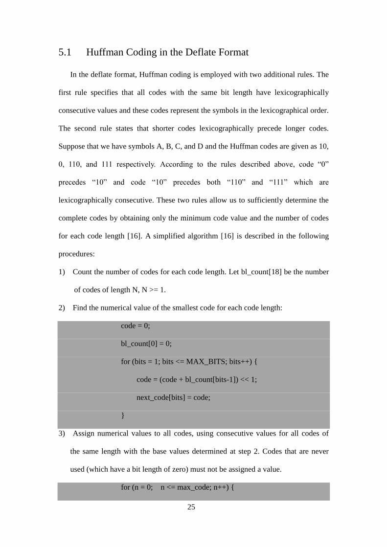
2) Find the numerical value of the smallest code for each code length:

code = 0;

bl_count[0] = 0;

for (bits = 1; bits <= MAX_BITS; bits++) {

code = (code + bl_count[bits-1]) << 1;

next_code[bits] = code;

}

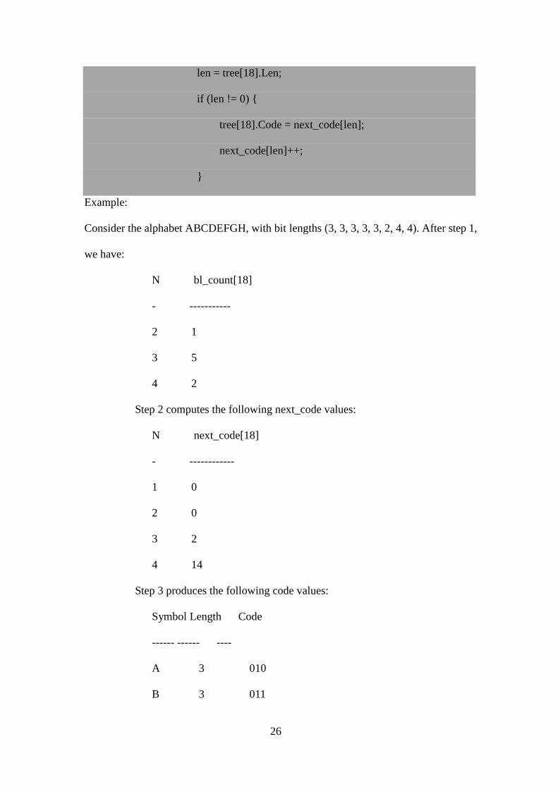
3) Assign numerical values to all codes, using consecutive values for all codes of

the same length with the base values determined at step 2. Codes that are never

used (which have a bit length of zero) must not be assigned a value.

for (n = 0; n <= max_code; n++) {

26

len = tree[18].Len;

if (len != 0) {

tree[18].Code = next_code[len];

next_code[len]++;

}

Example:

Consider the alphabet ABCDEFGH, with bit lengths (3, 3, 3, 3, 3, 2, 4, 4). After step 1,

we have:

N bl_count[18]

- -----------

2 1

3 5

4 2

Step 2 computes the following next_code values:

N next_code[18]

- ------------

1 0

2 0

3 2

4 14

Step 3 produces the following code values:

Symbol Length Code

------ ------ ----

A 3 010

B 3 011

27

C 3 100

D 3 101

E 3 110

F 2 00

G 4 1110

H 4 1111

5.2 LZ77-Related Compression Algorithm Details

The Lempel-Ziv 77 is the first compression algorithm for sequential data

compression. The dictionary of the LZ77 is a portion of the previously encoded

sequence. The encoder examines the input sequence through a sliding window as

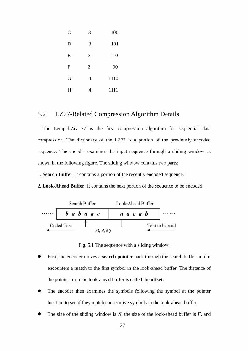
shown in the following figure. The sliding window contains two parts:

1. Search Buffer: It contains a portion of the recently encoded sequence.

2. Look-Ahead Buffer: It contains the next portion of the sequence to be encoded.

Fig. 5.1 The sequence with a sliding window.

First, the encoder moves a search pointer back through the search buffer until it

encounters a match to the first symbol in the look-ahead buffer. The distance of

the pointer from the look-ahead buffer is called the offset.

The encoder then examines the symbols following the symbol at the pointer

location to see if they match consecutive symbols in the look-ahead buffer.

The size of the sliding window is N, the size of the look-ahead buffer is F, and

28

the size of the search buffer is (N-F).

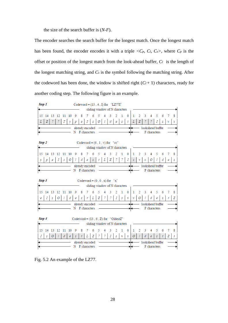
The encoder searches the search buffer for the longest match. Once the longest match

has been found, the encoder encodes it with a triple <Cp, Cl, Cs>, where Cp is the

offset or position of the longest match from the look-ahead buffer, Cl is the length of

the longest matching string, and Cs is the symbol following the matching string. After

the codeword has been done, the window is shifted right (Cl + 1) characters, ready for

another coding step. The following figure is an example.

Fig. 5.2 An example of the LZ77.

29

Chapter 6 HD Photo (JPEG XR)

Equation Chapter (Next) Section 1

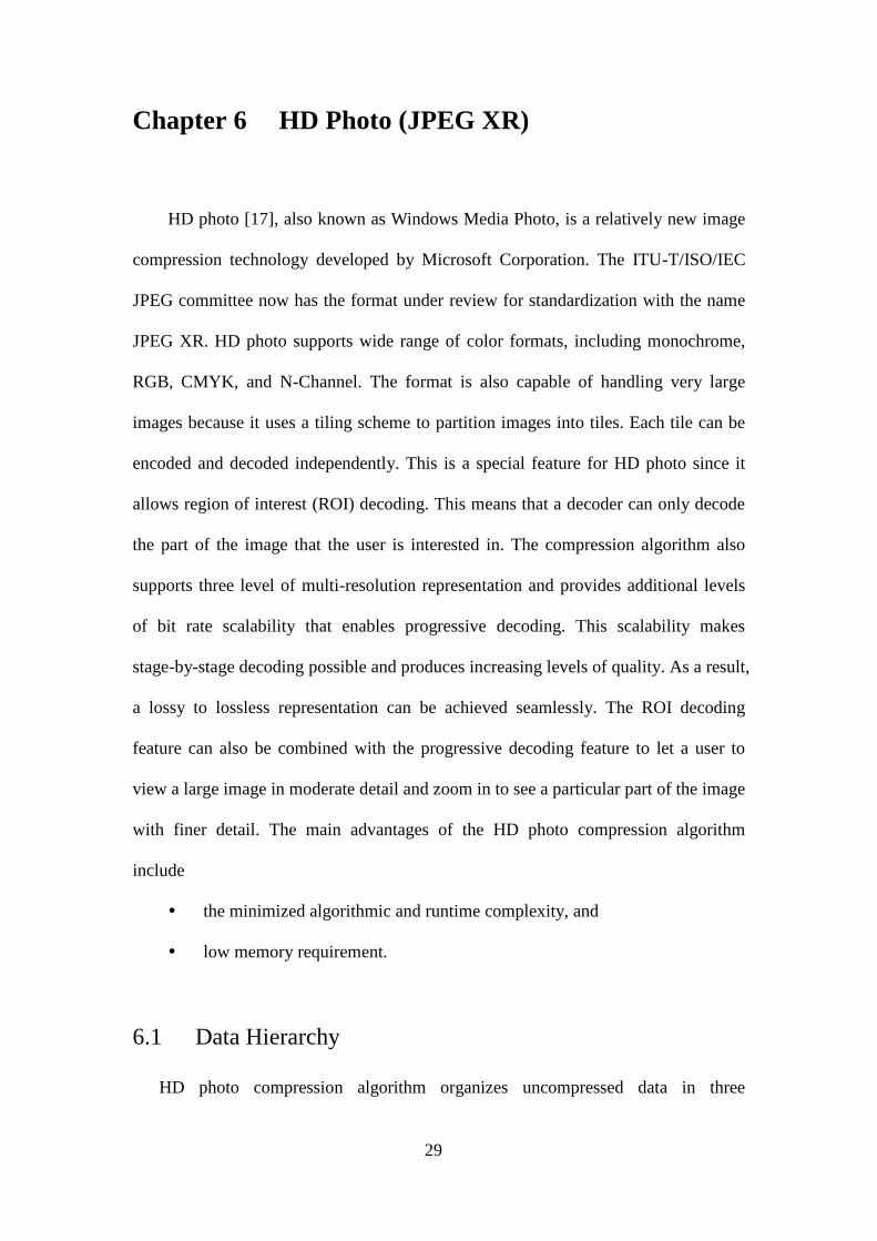
HD photo [17], also known as Windows Media Photo, is a relatively new image

compression technology developed by Microsoft Corporation. The ITU-T/ISO/IEC

JPEG committee now has the format under review for standardization with the name

JPEG XR. HD photo supports wide range of color formats, including monochrome,

RGB, CMYK, and N-Channel. The format is also capable of handling very large

images because it uses a tiling scheme to partition images into tiles. Each tile can be

encoded and decoded independently. This is a special feature for HD photo since it

allows region of interest (ROI) decoding. This means that a decoder can only decode

the part of the image that the user is interested in. The compression algorithm also

supports three level of multi-resolution representation and provides additional levels

of bit rate scalability that enables progressive decoding. This scalability makes

stage-by-stage decoding possible and produces increasing levels of quality. As a result,

a lossy to lossless representation can be achieved seamlessly. The ROI decoding

feature can also be combined with the progressive decoding feature to let a user to

view a large image in moderate detail and zoom in to see a particular part of the image

with finer detail. The main advantages of the HD photo compression algorithm

include

the minimized algorithmic and runtime complexity, and

low memory requirement.

6.1 Data Hierarchy

HD photo compression algorithm organizes uncompressed data in three

30

orthogonal dimensions: multiple color channels, hierarchical spatial layout, and

hierarchical frequency layout. All three dimensions are discussed in the following

sub-sections.

1) Color Channels: Unlike a YUV image that only has a luma plane and 2 chroma

channels, an HD photos supports a total of 16 color channels including one luma

channel and 15 chroma channels. In addition, an HD photo also contains an alpha

channel that controls the transparency of the image. For a YUV 4:4:4 compression

format, the spatial resolutions of all the color channels are the same. For a YUV

4:2:2 format, both the two chroma channels are downsampled by a factor of 2

horizontally. For a YUV 4:2:0 format, the same downsampling process is

performed in both vertical and horizontal directions.

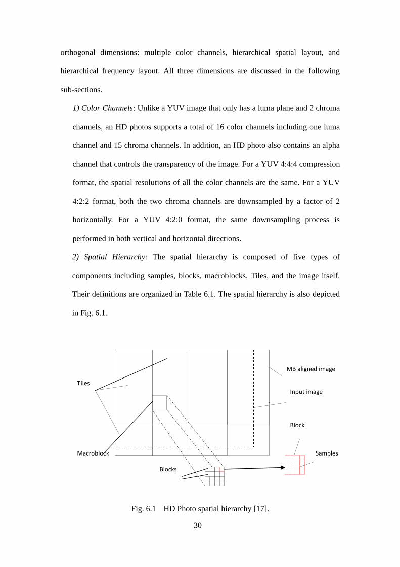
2) Spatial Hierarchy: The spatial hierarchy is composed of five types of

components including samples, blocks, macroblocks, Tiles, and the image itself.

Their definitions are organized in Table 6.1. The spatial hierarchy is also depicted

in Fig. 6.1.

Fig. 6.1 HD Photo spatial hierarchy [17].

Blocks

Macroblock

Block

Samples

Tiles

Input image

MB aligned image

31

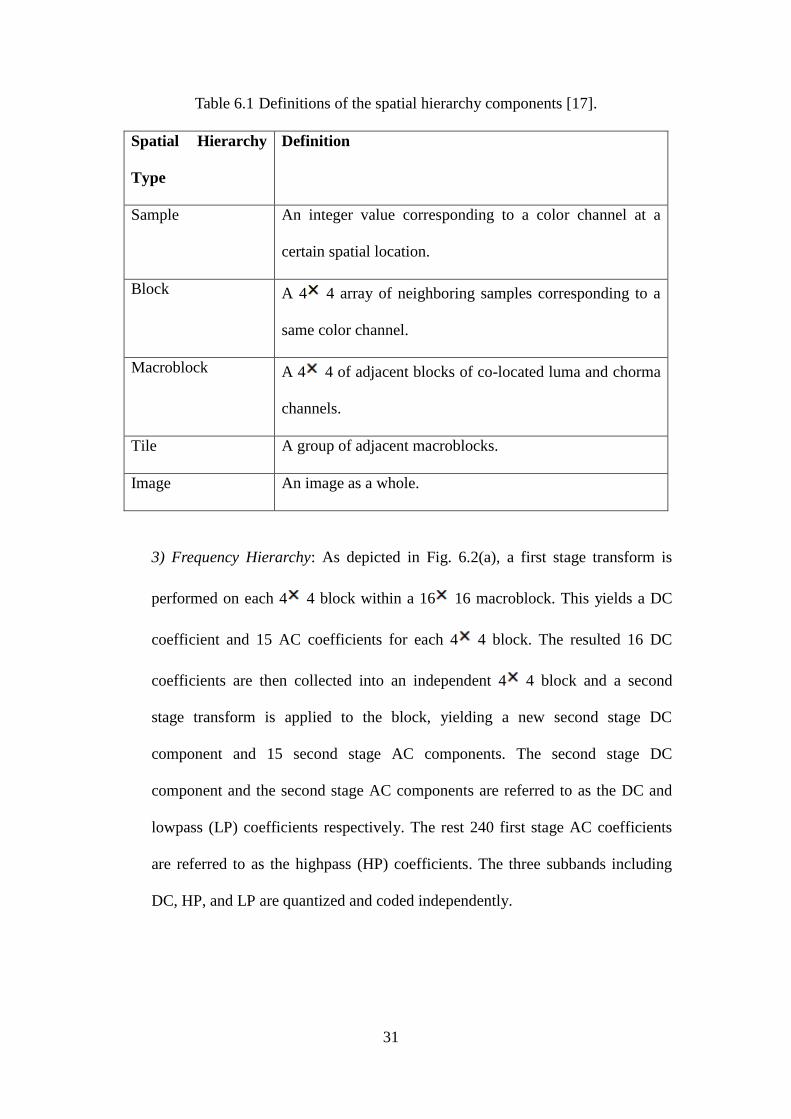
Table 6.1 Definitions of the spatial hierarchy components [17].

Spatial Hierarchy

Type

Definition

Sample An integer value corresponding to a color channel at a

certain spatial location.

Block A 4 4 array of neighboring samples corresponding to a

same color channel.

Macroblock A 4 4 of adjacent blocks of co-located luma and chorma

channels.

Tile A group of adjacent macroblocks.

Image An image as a whole.

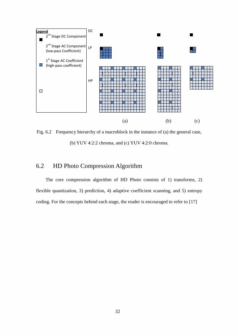
3) Frequency Hierarchy: As depicted in Fig. 6.2(a), a first stage transform is

performed on each 4 4 block within a 16 16 macroblock. This yields a DC

coefficient and 15 AC coefficients for each 4 4 block. The resulted 16 DC

coefficients are then collected into an independent 4 4 block and a second

stage transform is applied to the block, yielding a new second stage DC

component and 15 second stage AC components. The second stage DC

component and the second stage AC components are referred to as the DC and

lowpass (LP) coefficients respectively. The rest 240 first stage AC coefficients

are referred to as the highpass (HP) coefficients. The three subbands including

DC, HP, and LP are quantized and coded independently.

32

(a) (b) (c)

Fig. 6.2 Frequency hierarchy of a macroblock in the instance of (a) the general case,

(b) YUV 4:2:2 chroma, and (c) YUV 4:2:0 chroma.

6.2 HD Photo Compression Algorithm

The core compression algorithm of HD Photo consists of 1) transforms, 2)

flexible quantization, 3) prediction, 4) adaptive coefficient scanning, and 5) entropy

coding. For the concepts behind each stage, the reader is encouraged to refer to [17]

DC

LP

HP

Legend 2

nd Stage DC Component

2

nd Stage AC Component

(low-pass Coefficient)

1st

Stage AC Coefficient (high-pass coefficient)

33

Chapter 7 TIFF 6.0

Equation Chapter (Next) Section 1

TIFF (Tag Image File Format) [18] 6.0 is a raster file format that supports

bi-level, grayscale, palette-color, and full-color image data in several color spaces. It

usually describes image data from scanners, frame grabbers, and paint- and

photo-retouching programs. In TIFF 6.0, several compression schemes are employed

including the PackBits compression, the modified Huffman compression that adapts

the coding scheme of CCITT Group III and IV compression, and LZW compression.

However, this flexibility of compression scheme actually makes the file format itself

complicated because if some image readers are not able to decode any one of the

compressions used in the encoding process, decompression failures will occur.

7.1 Difference Predictor

A horizontal difference predictor [18] is applied before LZW to further improve

compression ratio. A difference predictor allows LZW to compact the data more

compactly due to the fact that many continuous-tone images do not have much

variation between the neighboring pixels. This means that many of the differences

should be 0, 1, or -1. The combination of LZW coding with horizontal differencing is

lossless.

7.2 PackBits Compression

The Apple Macintosh PackBits compression algorithm [19], [18] is a simple

byte-oriented run-length encoding (RLE) scheme. The PackBits scheme specifies that

the length of uncompressed data must not be greater than 127 bytes. If the

34

uncompressed data to be compressed is more than 127 bytes, the data is broken up

into 127-byte groups and the PackBits compression is then performed on each group.

In the encoding data, the first byte that belongs to two’s compliment system is a

flag-counter byte that indicates whether the consequent data is packed or not and the

number of bytes in the packed or unpacked data. If this first byte is a negative number,

the following data is packed and the number is a zero-based count of the number of

times the data byte repeats when expanded. There is one data byte following the

flag-counter byte in packed data; the byte after the data byte is the next flag-counter

byte. If the flag-counter byte is a positive number, then the following data is unpacked

and the number is a zero-based count of the number of incompressible data bytes that

follow. There are (flag-counter+1) data bytes following the flag-counter byte. The

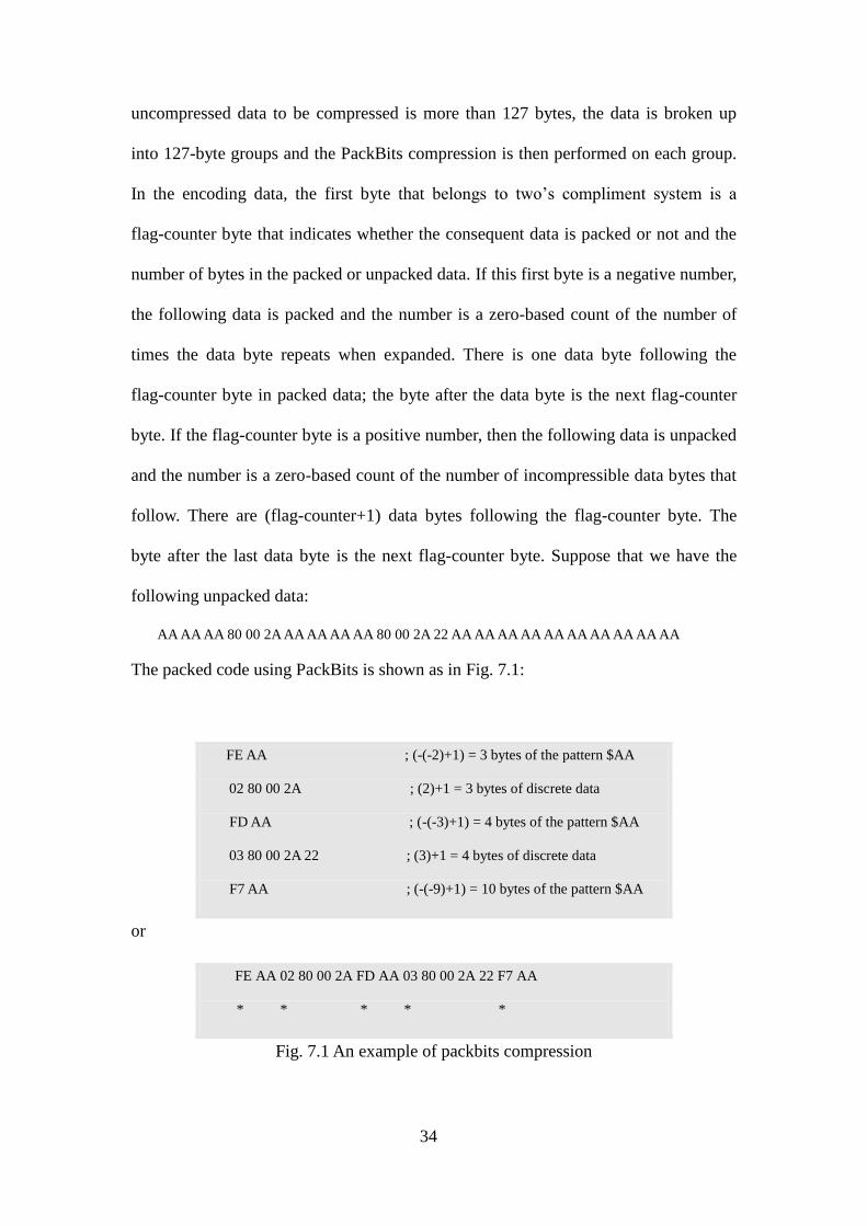
byte after the last data byte is the next flag-counter byte. Suppose that we have the

following unpacked data:

AA AA AA 80 00 2A AA AA AA AA 80 00 2A 22 AA AA AA AA AA AA AA AA AA AA

The packed code using PackBits is shown as in Fig. 7.1:

FE AA ; (-(-2)+1) = 3 bytes of the pattern $AA

02 80 00 2A ; (2)+1 = 3 bytes of discrete data

FD AA ; (-(-3)+1) = 4 bytes of the pattern $AA

03 80 00 2A 22 ; (3)+1 = 4 bytes of discrete data

F7 AA ; (-(-9)+1) = 10 bytes of the pattern $AA

or

FE AA 02 80 00 2A FD AA 03 80 00 2A 22 F7 AA

* * * * *

Fig. 7.1 An example of packbits compression

35

The bytes with the asterisk (*) under them are the flag-counter bytes. PackBits packs

the data only when there are three or more consecutive bytes with the same data;

otherwise it just copies the data byte for byte (and adds the count byte). During the

unpacking process, the process must require the length of the unpacked data in order

to know that the process have reached the end of the packed data [19].

7.3 Modified Huffman Compression

The modified Huffman compression [18] is based on the CCITT Group 3 1D

facsimile compression scheme and it is used for processing bi-level data. Since the

modified Huffman compression is a method for encoding bi-level images, code words

are only used to represent the run length of the alternative black and white runs. In

order to maintain color synchronization at the decompressing side, every single data

line starts with a white run-length code word set. A white run of zero run-length is

sent in the case of an initial black run. All the usable code words are completely

shown in [18] under section 10. The code words are of two types: Terminating code

words and Make-up code words. Each run-length is represented by zero or more

Make-up code words followed by exactly one Terminating code word. Run lengths in

the range of 0 to 63 pixels are encoded with their appropriate Terminating code word.

If run lengths are bigger than 63, the run-length is encoded with Make-up code words

followed by a Terminated code word. For example, if the run-length is 2623, the

run-length is separated into 2560 and 63 that are coded by a Make-up code word and a

Terminated code word respectively.

36

Chapter 8 Conclusion and Comparison

The compression standards have been introduced. We are not difficult to notice

that, for lossy compression, there must be sacrifice in quality while raising

compression ratio. On the other hand, compression ratio in lossless compression is

much worse than in lossy one. What researchers try to investigate is creating a method

with high compression ratio and less distortion. However, as discussed above, every

compression standard has its own applications, such as bi-level image or 8-bits per

pixel image, so it has different performance when dealing with different types of

images. Nowadays there therefore is still no method to include all these compression

standards and techniques.

37

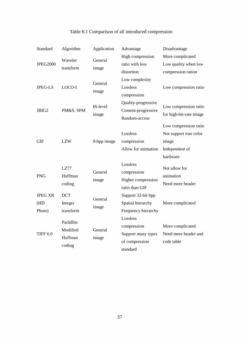
Table 8.1 Comparison of all introduced compression

Standard Algorithm Application Advantage Disadvantage

JPEG2000 Wavelet

transform

General

image

High compression

ratio with less

distortion

More complicated

Low quality when low

compression ration

JPEG-LS LOCO-I General

image

Low complexity

Lossless

compression

Low compression ratio

JBIG2 PM&S, SPM Bi-level

image

Quality-progressive

Content-progressive

Random-access

Low compression ratio

for high-bit-rate image

GIF LZW 8-bpp image

Lossless

compression

Allow for animation

Low compression ratio

Not support true color

image

Independent of

hardware

PNG

LZ77

Huffman

coding

General

image

Lossless

compression

Higher compression

ratio than GIF

Not allow for

animation

Need more header

JPEG XR

(HD

Photo)

DCT

Integer

transform

General

image

Support 32-bit bpp

Spatial hierarchy

Frequency hierarchy

More complicated

TIFF 6.0

PackBits

Modified

Huffman

coding

General

image

Lossless

compression

Support many types

of compression

standard

More complicated

Need more header and

code table

38

REFERENCES

A. Digital Image Processing

[1] R. C. Gonzalez and R. E. Woods, Digital Image Processing Second Ed., Prentice

Hall, New Jersey, 2002.

[2] X. Wu and N. D. Memon, “Context-based, adaptive, lossless image coding,”

IEEE Trans. Commun., vol. 45, pp. 437-444, Apr. 1997.

B. Digital Image Compression

[3] 酒井善則、吉田俊之 共著，白執善 編譯，“影像壓縮技術”，全華，2004

[4] T. Acharya amd A. K. Ray, Image Processing Principles and Applications, John

Wiley & Sons, New Jersey.

[5] C. Christopoulos, A. Skodras, and T. Ebrahimi, “The JPEG2000 Still Image

Coding System: An Overview, ”IEEE Trans. on Consumer Electronics, vol. 46,

no. 4, pp.1103-1127, Nov. 2000.

[6] M. Rabbani and R. Joshi, “An Overview of the JPEG2000 Still Image

Compression Standard,” Signal Processing: Image Comm., vol. 17, no. 1, 2002.

[7] S. G. Mallat, "A theory for multiresolution signal decomposition: the wavelet

representation," Transactions on Pattern Analysis and Machine Intelligence,

vol.11, no.7, pp.674-693, Jul. 1989.

[8] M.J. Slattery, J.L. Mitchell, “The Qx-coder,” IBM J. Res. Development, vol. 42,

no. 6, pp. 767–784, Nov. 1998.

C. Other Existing Compression Standards of Still Images and Their Coding

Details

39

[9] Nasir D. Memon, Xiaolin Wu, V. Sippy, and G. Miller, “Interband coding

extension of the new lossless JPEG standard,” Proc. SPIE Int. Soc. Opt. Eng., vol.

3024, no. 47, pp.47-58, Jan. 1997.

[10] M. J. Weinberger, G. Seroussi, and G. Sapiro, “LOCO-I: A low complexity,

context-based, lossless image compression algorithm,” in Proc. 1996 Data

Compression Conference, pp. 140–149, Snowbird, UT, Mar. 1996.

[11] M. Weinberger, G. Seroussi, and G. Sapiro, “The LOCO-I lossless image

compression algorithm: Principles and standardization into JPEG-LS,” IEEE

Trans. Image Processing, vol. 9, no. 8, pp. 1309–1324, Aug. 2000, originally as

Hewlett-Packard Laboratories Technical Report No. HPL-98-193R1, November

1998, revised October 1999. Available from http://www.hpl.hp.com/loco/.

[12] F. Ono, W. Rucklidge, R. Arps, and C. Constantinescu, "JBIG2-the ultimate

bi-level image coding standard," Image Processing, 2000. Proceedings. 2000

International Conference on , vol.1, pp.140-143, 2000.

[13] P. Howard, F. Kossentini, B. Martins, S. Forchhammer, and W. Rucklidge, "The

emerging JBIG2 standard," Circuits and Systems for Video Technology, IEEE

Transactions on, vol.8, no.7, pp.838-848, Nov 1998.

[14] M. Nelson, “LZW data compression,” Dr. Dobb’s Journal, pp. 29-36, 86-87, Oct.

1989.

[15] G. Randers-Pehrson et al., PNG (Portable Network Graphics) specification

version 1.2,” PNG Development Group, July 1999.

[16] P. Deutsch, DEFLATE Compressed Data Format Specification version 1.3, IETF

RFC 1951, May 1996; www.ietf.org/rfc/rfc1951.txt.

[17] S. Srinivasan, C. Tu, S. L. Regunathan, R. A. Rossi, Jr., G. J. Sullivan, “HD

Photo: a new image coding technology for digital photography,” Applications of

40

Digital Image Processing XXX, Proceedings of SPIE, vol. 6696, pp. 66960A,

August 2007.

[18] Adobe Systems. TIFF Specification, Revision 6.0. Available:

http://partners.adobe.com/public/developer/en/tiff/TIFF6.pdf.

[19] Apple Inc., "Understanding PackBits," Developer Connection, Apple Inc., Tech.

Note TN1023, 1996.