School of Mechanical EngineeringChung-Ang UniversityNumerical Methods 2010-2

Numerical DifferentiationNumerical Differentiation

Prof. Prof. HaeHae--Jin ChoiJin Choi

hjchoi@cau.ac.krhjchoi@cau.ac.kr

Part 5Part 5Chapter 19Chapter 19

1

School of Mechanical EngineeringChung-Ang UniversityNumerical Methods 2010-2

Chapter ObjectivesChapter Objectives

2

l Understanding the application of high-accuracy numerical differentiation formulas for equispaced data.

l Knowing how to evaluate derivatives for unequally spaced data.l Understanding how Richardson extrapolation is applied for

numerical differentiation.l Recognizing the sensitivity of numerical differentiation to data

error.l Knowing how to evaluate derivatives in MATLAB with the diff and

gradient functions.l Knowing how to generate contour plots and vector fields with

MATLAB.

School of Mechanical EngineeringChung-Ang UniversityNumerical Methods 2010-2

Introduction to DifferentiationIntroduction to Differentiation

3

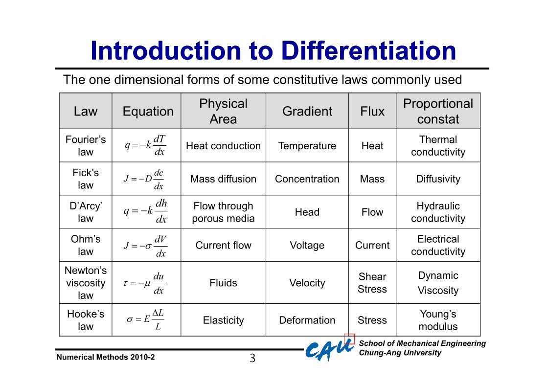
The one dimensional forms of some constitutive laws commonly used

Law Equation Physical Area Gradient Flux Proportional

constatFourier’s

law Heat conduction Temperature Heat Thermalconductivity

Fick’slaw Mass diffusion Concentration Mass Diffusivity

D’Arcy’ law

Flow throughporous media Head Flow Hydraulic

conductivity

Ohm’s law Current flow Voltage Current Electrical

conductivity

Newton’s viscosity

lawFluids Velocity Shear

StressDynamicViscosity

Hooke’s law Elasticity Deformation Stress Young’s

modulus

dVJdx

s= -

dcJ Ddx

= -

dTq kdx

= -

dhq kdx

= -

dudx

t m= -

LEL

s D=

School of Mechanical EngineeringChung-Ang UniversityNumerical Methods 2010-2

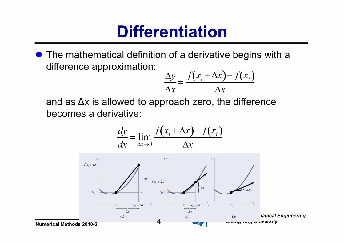
DifferentiationDifferentiationl The mathematical definition of a derivative begins with a

difference approximation:

and as Δx is allowed to approach zero, the difference becomes a derivative:

�

DyDx

=f xi + Dx( )- f xi( )

Dx

�

dydx

= limDx®0

f xi + Dx( )- f xi( )Dx

4

School of Mechanical EngineeringChung-Ang UniversityNumerical Methods 2010-2

HighHigh--Accuracy Differentiation Accuracy Differentiation FormulasFormulas

5

l Taylor series expansion can be used to generate high-accuracy formulas for derivatives by using linear algebra to combine the expansion around several points.

l Three categories for the formula include forward finite-difference, backward finite-difference, and centered finite-difference.

School of Mechanical EngineeringChung-Ang UniversityNumerical Methods 2010-2

Differentiation derived Differentiation derived from Taylor series expansionsfrom Taylor series expansions

6

l There are forward difference, backward difference and centered difference approximations, depending on the points used:

l Forward:

l Backward:

l Centered:

�

f '(x i) =f (x i+1) - f (x i)

h+ O(h)

�

f '(x i) =f (x i) - f (x i-1)

h+ O(h)

�

f '(x i) =f (x i+1) - f (x i-1)

2h+ O(h2)

School of Mechanical EngineeringChung-Ang UniversityNumerical Methods 2010-2

High Accuracy DifferentiationHigh Accuracy Differentiation

7

21

( )( ) ( ) ( )2!

ii i i

f xf x f x f x h h+

¢¢¢= + + +L

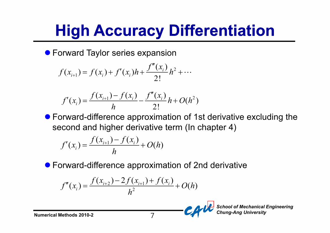
l Forward Taylor series expansion

21( ) ( ) ( )( ) ( )2!

i i ii

f x f x f xf x h O hh

+ ¢¢-¢ = - +

l Forward-difference approximation of 1st derivative excluding the second and higher derivative term (In chapter 4)

1( ) ( )( ) ( )i ii

f x f xf x O hh

+ -¢ = +

l Forward-difference approximation of 2nd derivative

2 12

( ) 2 ( ) ( )( ) ( )i i ii

f x f x f xf x O hh

+ +- +¢¢ = +

School of Mechanical EngineeringChung-Ang UniversityNumerical Methods 2010-2

High Accuracy DifferentiationHigh Accuracy Differentiation

8

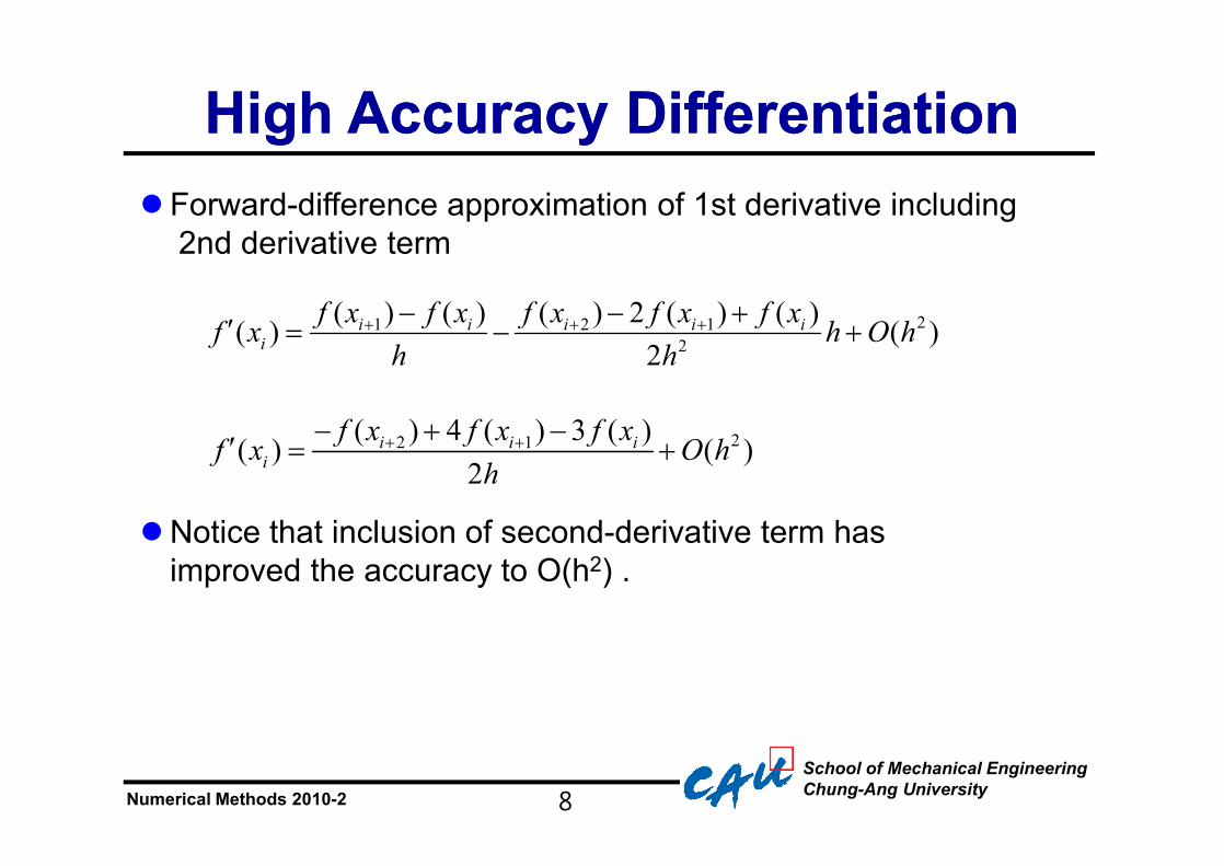
l Forward-difference approximation of 1st derivative including 2nd derivative term

21 2 12

( ) ( ) ( ) 2 ( ) ( )( ) ( )2

i i i i ii

f x f x f x f x f xf x h O hh h

+ + +- - +¢ = - +

22 1( ) 4 ( ) 3 ( )( ) ( )2

i i ii

f x f x f xf x O hh

+ +- + -¢ = +

lNotice that inclusion of second-derivative term has improved the accuracy to O(h2) .

School of Mechanical EngineeringChung-Ang UniversityNumerical Methods 2010-2

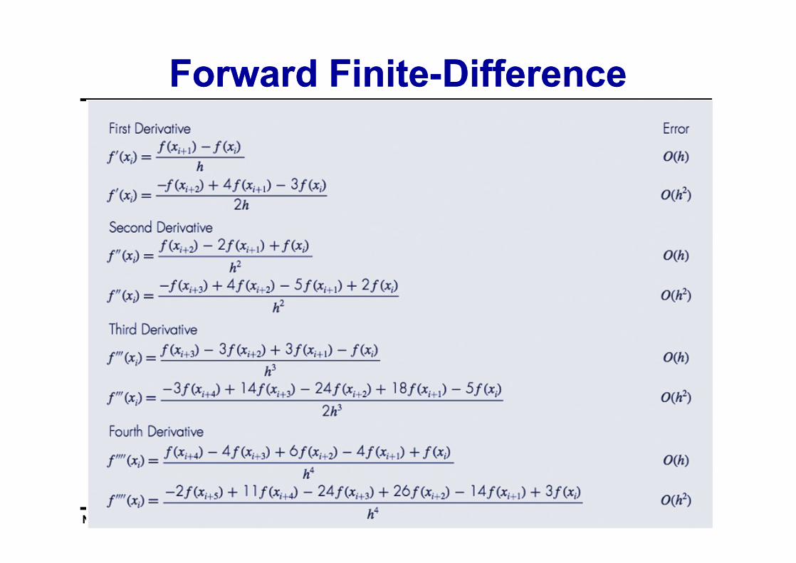
Forward FiniteForward Finite--DifferenceDifference

9

School of Mechanical EngineeringChung-Ang UniversityNumerical Methods 2010-2

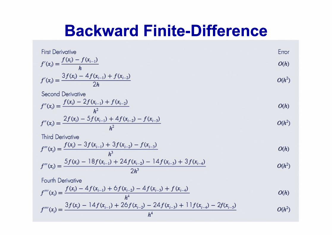
Backward FiniteBackward Finite--DifferenceDifference

10

School of Mechanical EngineeringChung-Ang UniversityNumerical Methods 2010-2

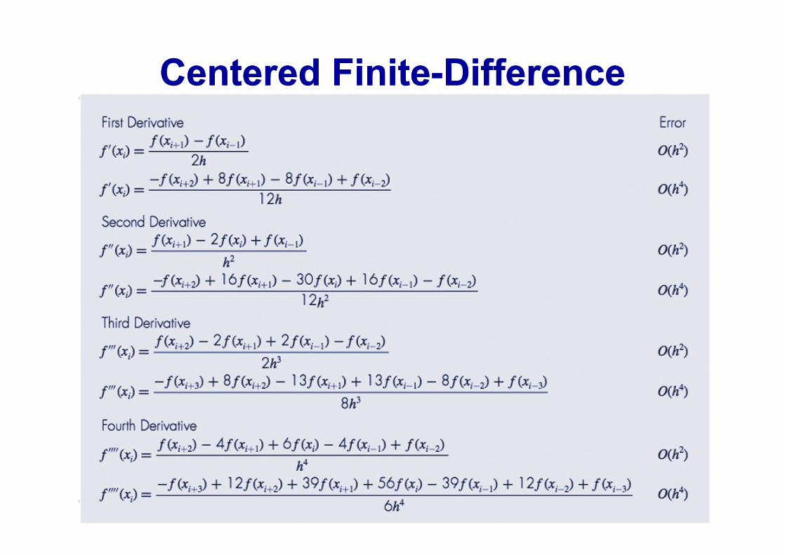
Centered FiniteCentered Finite--DifferenceDifference

11

School of Mechanical EngineeringChung-Ang UniversityNumerical Methods 2010-2

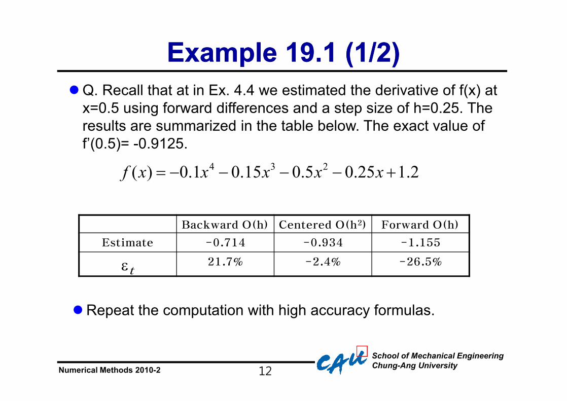
Example 19.1 (1/2)Example 19.1 (1/2)

12

lQ. Recall that at in Ex. 4.4 we estimated the derivative of f(x) at x=0.5 using forward differences and a step size of h=0.25. The results are summarized in the table below. The exact value of f’(0.5)= -0.9125.

4 3 2( ) 0.1 0.15 0.5 0.25 1.2f x x x x x= - - - - +

Backward O(h) Centered O(h2) Forward O(h)

Estimate -0.714 -0.934 -1.155

et21.7% -2.4% -26.5%

lRepeat the computation with high accuracy formulas.

School of Mechanical EngineeringChung-Ang UniversityNumerical Methods 2010-2

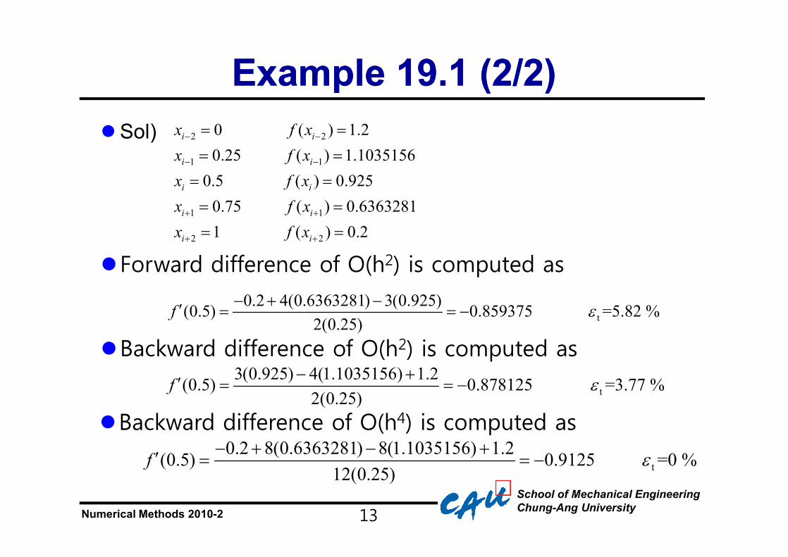
Example 19.1 (2/2)Example 19.1 (2/2)

13

lSol) 2 2

1 1

1 1

2 2

0 ( ) 1.20.25 ( ) 1.1035156

0.5 ( ) 0.9250.75 ( ) 0.63632811 ( ) 0.2

i i

i i

i i

i i

i i

x f xx f xx f xx f xx f x

- -

- -

+ +

+ +

= =

= =

= =

= =

= =

lForward difference of O(h2) is computed as

t0.2 4(0.6363281) 3(0.925)(0.5) 0.859375 =5.82 %

2(0.25)f e- + -¢ = = -

lBackward difference of O(h2) is computed as

t3(0.925) 4(1.1035156) 1.2(0.5) 0.878125 =3.77 %

2(0.25)f e- +¢ = = -

lBackward difference of O(h4) is computed as

t0.2 8(0.6363281) 8(1.1035156) 1.2(0.5) 0.9125 =0 %

12(0.25)f e- + - +¢ = = -

School of Mechanical EngineeringChung-Ang UniversityNumerical Methods 2010-2

Richardson ExtrapolationRichardson Extrapolation

14

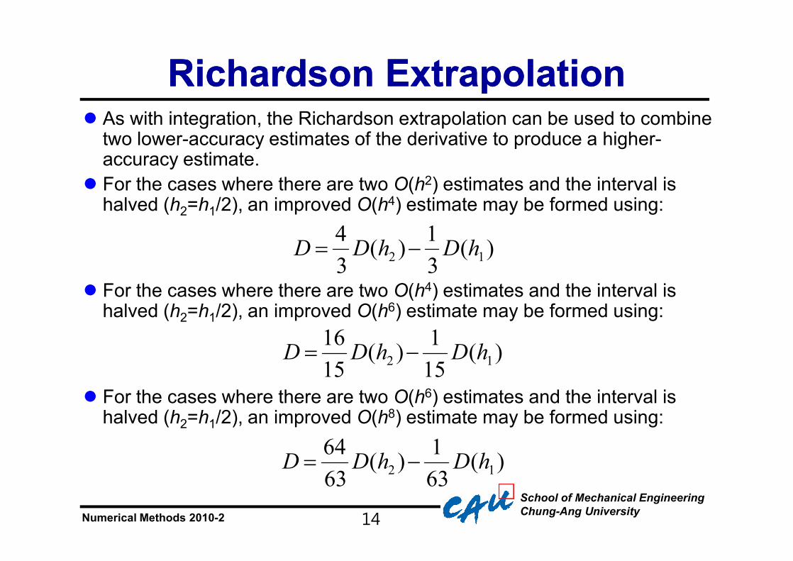
l As with integration, the Richardson extrapolation can be used to combine two lower-accuracy estimates of the derivative to produce a higher-accuracy estimate.

l For the cases where there are two O(h2) estimates and the interval is halved (h2=h1/2), an improved O(h4) estimate may be formed using:

l For the cases where there are two O(h4) estimates and the interval is halved (h2=h1/2), an improved O(h6) estimate may be formed using:

l For the cases where there are two O(h6) estimates and the interval is halved (h2=h1/2), an improved O(h8) estimate may be formed using:

�

D =43

D(h2 ) -13

D(h1)

�

D =1615

D(h2 ) -1

15D(h1)

�

D =6463

D(h2 ) -163

D(h1)

School of Mechanical EngineeringChung-Ang UniversityNumerical Methods 2010-2

Example 19.2Example 19.2

15

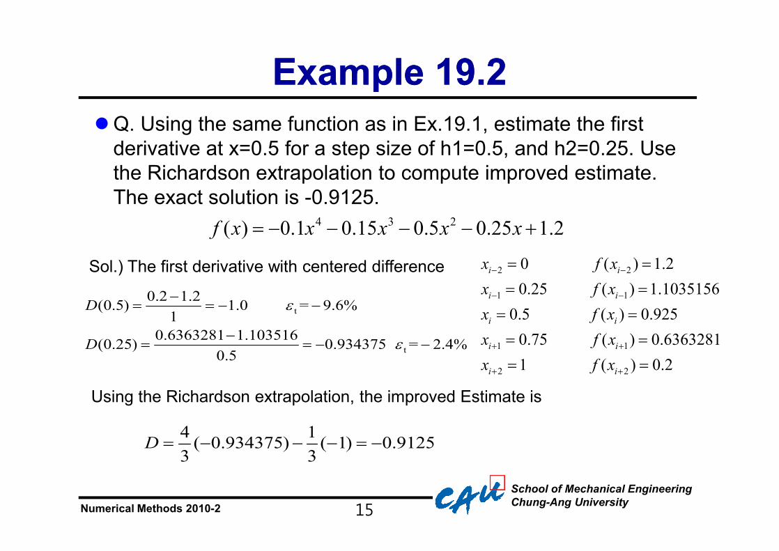
lQ. Using the same function as in Ex.19.1, estimate the first derivative at x=0.5 for a step size of h1=0.5, and h2=0.25. Use the Richardson extrapolation to compute improved estimate. The exact solution is -0.9125.

4 3 2( ) 0.1 0.15 0.5 0.25 1.2f x x x x x= - - - - +

Sol.) The first derivative with centered difference 2 2

1 1

1 1

2 2

0 ( ) 1.20.25 ( ) 1.1035156

0.5 ( ) 0.9250.75 ( ) 0.63632811 ( ) 0.2

i i

i i

i i

i i

i i

x f xx f xx f xx f xx f x

- -

- -

+ +

+ +

= =

= =

= =

= =

= =

t

t

0.2 1.2(0.5) 1.0 = 9.6%1

0.6363281 1.103516(0.25) 0.934375 = 2.4%0.5

D

D

e

e

-= = - -

-= = - -

Using the Richardson extrapolation, the improved Estimate is

4 1( 0.934375) ( 1) 0.9125 3 3

D = - - - = -

School of Mechanical EngineeringChung-Ang UniversityNumerical Methods 2010-2

Unequally Spaced DataUnequally Spaced Data

16

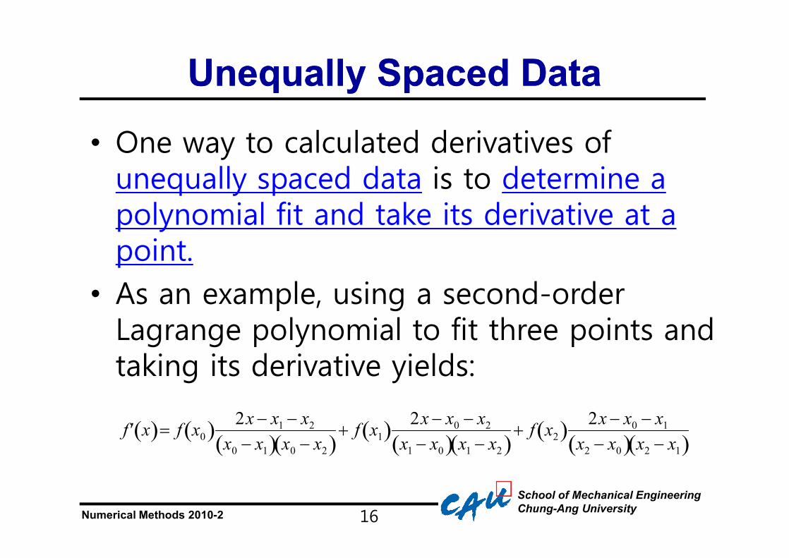
• One way to calculated derivatives of unequally spaced data is to determine a polynomial fit and take its derivative at a point.

• As an example, using a second-order Lagrange polynomial to fit three points and taking its derivative yields:

�

¢ f x( )= f x0( ) 2x - x1 - x2

x0 - x1( ) x0 - x2( )+ f x1( ) 2x - x0 - x2

x1 - x0( ) x1 - x2( )+ f x2( ) 2x - x0 - x1

x2 - x0( ) x2 - x1( )

School of Mechanical EngineeringChung-Ang UniversityNumerical Methods 2010-2

Example 19.3Example 19.3

17

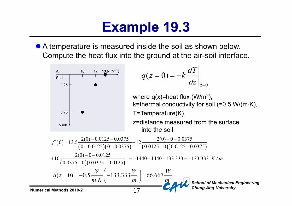
lA temperature is measured inside the soil as shown below. Compute the heat flux into the ground at the air-soil interface.

0

( 0)z

dTq z kdz =

= = -

where q(x)=heat flux (W/m2), k=thermal conductivity for soil (=0.5 W/(m·K),T=Temperature(K), z=distance measured from the surface

into the soil.

( ) ( )( ) ( )( )

( )( )

2(0) 0.0125 0.0375 2(0) 0 0.03750 13.5 120 0.0125 0 0.0375 0.0125 0 0.0125 0.0375

2(0) 0 0.012510 1440 1440 133.333 133.333 /0.0375 0 0.0375 0.0125

f

K m

- - - -¢ = +- - - -

- -+ = - + - = -

- -

2( 0) 0.5 133.333 66.667

W W Wq zm K m m

æ ö= = - - =ç ÷è ø

School of Mechanical EngineeringChung-Ang UniversityNumerical Methods 2010-2

Derivatives and Integrals for Derivatives and Integrals for Data with ErrorsData with Errors

18

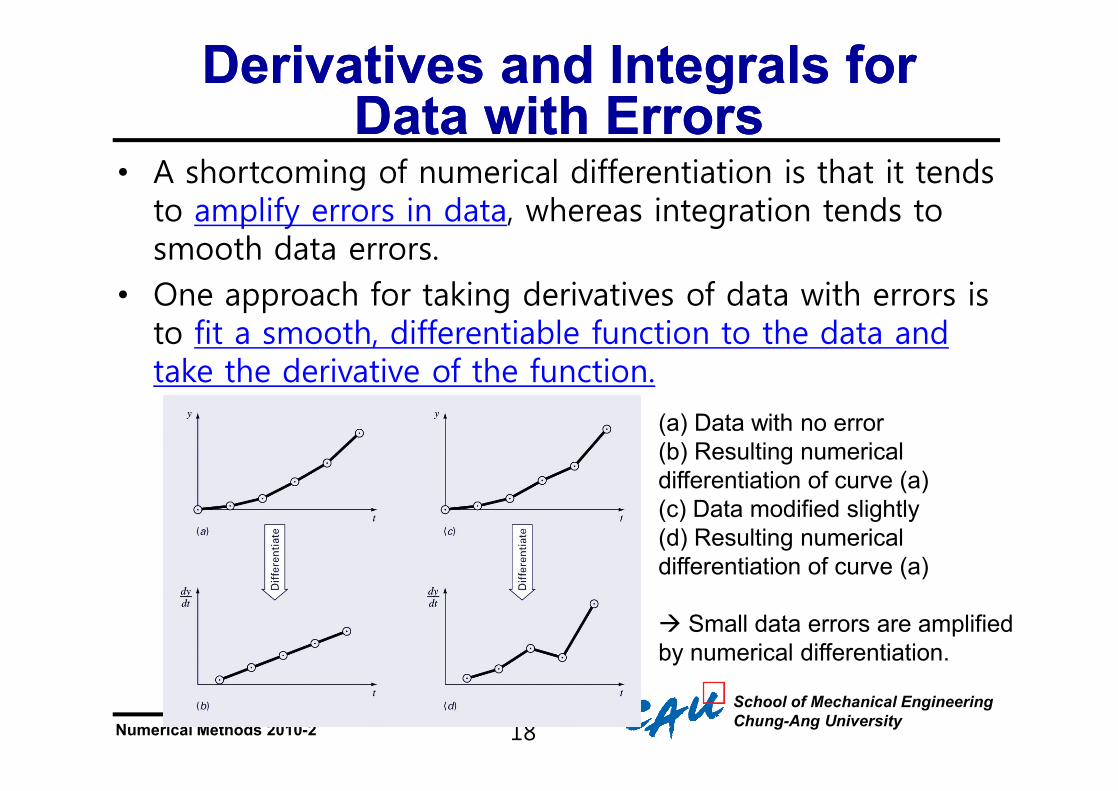
• A shortcoming of numerical differentiation is that it tends to amplify errors in data, whereas integration tends to smooth data errors.

• One approach for taking derivatives of data with errors is to fit a smooth, differentiable function to the data and take the derivative of the function.

(a) Data with no error(b) Resulting numericaldifferentiation of curve (a)(c) Data modified slightly(d) Resulting numericaldifferentiation of curve (a)

à Small data errors are amplifiedby numerical differentiation.

School of Mechanical EngineeringChung-Ang UniversityNumerical Methods 2010-2

Numerical Differentiation with Numerical Differentiation with MATLABMATLAB

19

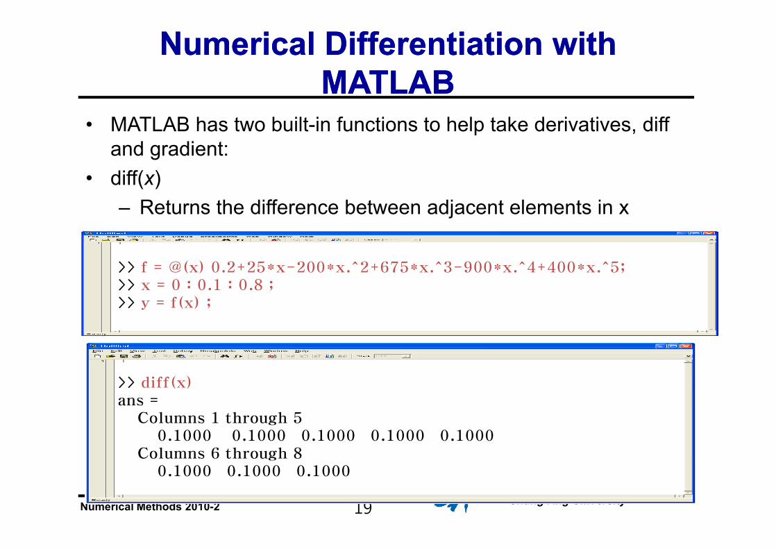
• MATLAB has two built-in functions to help take derivatives, diff and gradient:

• diff(x)– Returns the difference between adjacent elements in x

>> f = @(x) 0.2+25*x-200*x.^2+675*x.^3-900*x.^4+400*x.^5;>> x = 0 : 0.1 : 0.8 ;>> y = f(x) ;

>> diff(x)ans =

Columns 1 through 50.1000 0.1000 0.1000 0.1000 0.1000

Columns 6 through 80.1000 0.1000 0.1000

School of Mechanical EngineeringChung-Ang UniversityNumerical Methods 2010-2

Numerical Differentiation with Numerical Differentiation with MATLABMATLAB

20

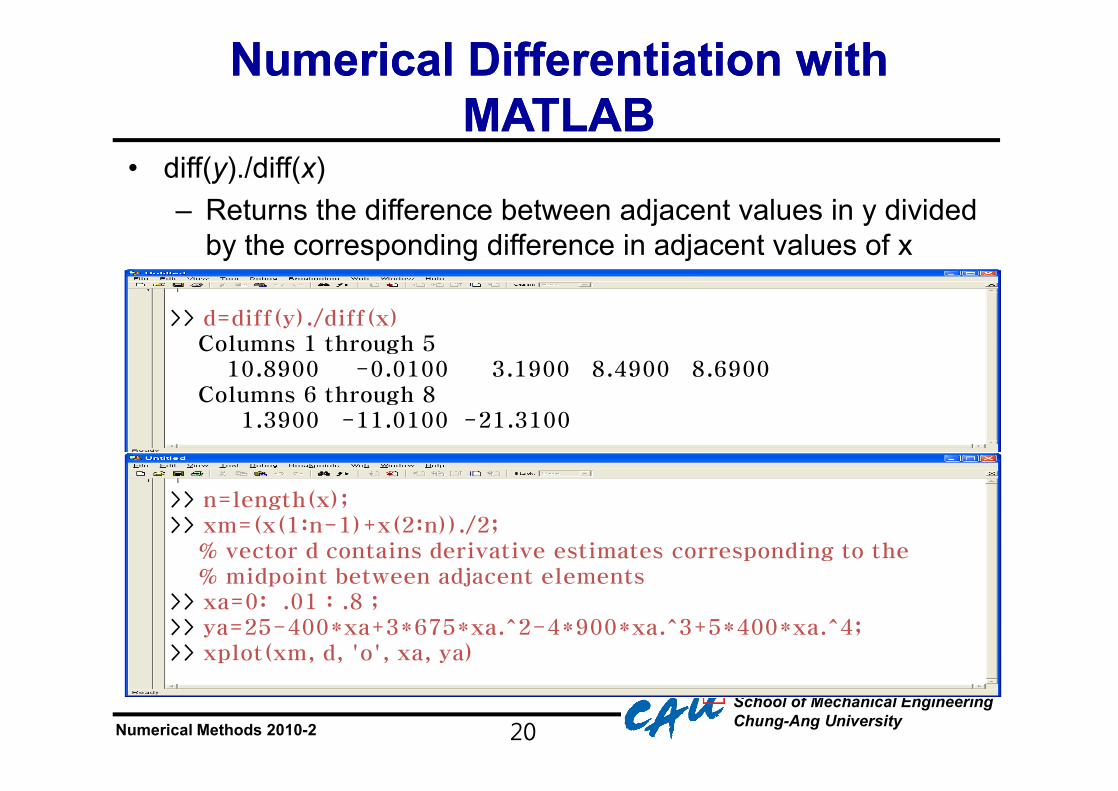
• diff(y)./diff(x)– Returns the difference between adjacent values in y divided

by the corresponding difference in adjacent values of x

>> d=diff(y)./diff(x) Columns 1 through 5

10.8900 -0.0100 3.1900 8.4900 8.6900Columns 6 through 8

1.3900 -11.0100 -21.3100

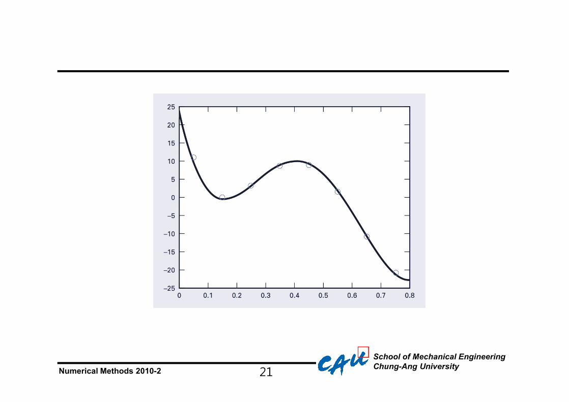
>> n=length(x);>> xm=(x(1:n-1)+x(2:n))./2;

% vector d contains derivative estimates corresponding to the % midpoint between adjacent elements

>> xa=0: .01 : .8 ;>> ya=25-400*xa+3*675*xa.^2-4*900*xa.^3+5*400*xa.^4;>> xplot(xm, d, 'o', xa, ya)

School of Mechanical EngineeringChung-Ang UniversityNumerical Methods 2010-2 21

School of Mechanical EngineeringChung-Ang UniversityNumerical Methods 2010-2

Numerical Differentiation with Numerical Differentiation with MATLABMATLAB

22

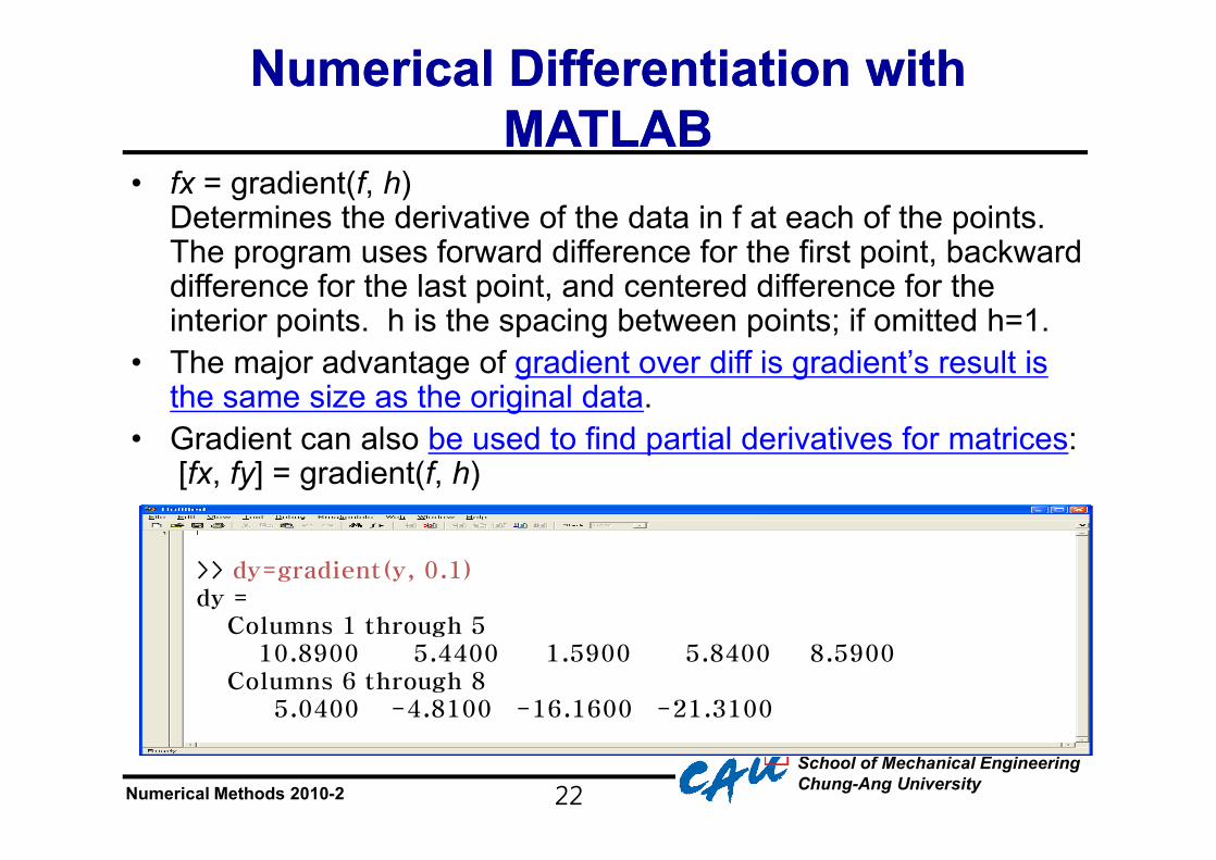
• fx = gradient(f, h)Determines the derivative of the data in f at each of the points. The program uses forward difference for the first point, backward difference for the last point, and centered difference for the interior points. h is the spacing between points; if omitted h=1.

• The major advantage of gradient over diff is gradient’s result is the same size as the original data.

• Gradient can also be used to find partial derivatives for matrices:[fx, fy] = gradient(f, h)

>> dy=gradient(y, 0.1)dy =

Columns 1 through 510.8900 5.4400 1.5900 5.8400 8.5900

Columns 6 through 85.0400 -4.8100 -16.1600 -21.3100

School of Mechanical EngineeringChung-Ang UniversityNumerical Methods 2010-2 23

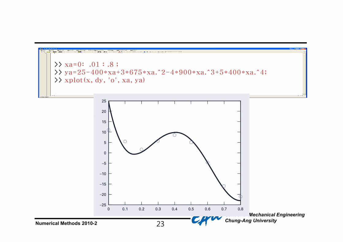
>> xa=0: .01 : .8 ;>> ya=25-400*xa+3*675*xa.^2-4*900*xa.^3+5*400*xa.^4;>> xplot(x, dy, 'o', xa, ya)