Embed Size (px)
Citation preview
Particle Physics of the Early Universe
Alexey BoyarskySpring semester 2015
Fermi theory of β-decay 1
Continuumspectrum ofelectrons(1927)
Prediction ofneutrino(1930, 1934)
Fermi theory(1934)
Universality ofFermiinteractions(1949)
� Neutron decay n→ p+ e− + νe
� Two papers by E. Fermi:
An attempt of a theory of beta radiation. 1. (InGerman) Z.Phys. 88 (1934) 161-177
DOI: 10.1007/BF01351864
Trends to a Theory of beta Radiation. (InItalian) Nuovo Cim. 11 (1934) 1-19
DOI: 10.1007/BF02959820
� Fermi 4-fermion theory:
LFermi = −GF√2
[p(x)γµn(x)][e(x)γµν(x)] (1)
0History of β-decay (see [hep-ph/0001283], Sec. 1,1); Cheng & Li, Chap. 11, Sec. 11.1)
Alexey Boyarsky PPEU 2015 1
Neutrino-electron scattering
� Fermi Lagrangian includes leptonic and hardronic terms:
LFermi = −GF√2
[J†lepton(x) + J†hadron(x)
]·[Jlepton(x) + Jhadron(x)
](2)
where current Jµ has leptonic (e±, µ±, ν, ν) and hadronic (p, n, π)parts
� Fermi theory predicts lepton-only weak interactions, such as e +νe → e+ νe scattering
Lνe =4GF√
2(eγλνe)(νeγ
λe) (3)
� Matrix element for e+ νe → e+ νe scattering
∑spins
|M|2 ∝ G2FE
4c.m. (4)
Alexey Boyarsky PPEU 2015 2
Massive intermediate particle
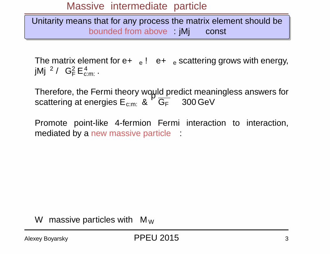
Unitarity means that for any process the matrix element should bebounded from above: |M| ≤ const
� The matrix element for e+νe → e+νe scattering grows with energy,|M|2 ∝ G2
FE4c.m..
� Therefore, the Fermi theory would predict meaningless answers forscattering at energies Ec.m. &
√GF ≈ 300 GeV
� Promote point-like 4-fermion Fermi interaction to interaction,mediated by a new massive particle :
� W – massive particles with MW
Alexey Boyarsky PPEU 2015 3
Massive intermediate particle
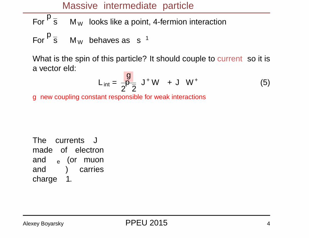
� For√s�MW – looks like a point, 4-fermion interaction
� For√s�MW – behaves as s−1
� What is the spin of this particle? It should couple to current so it isa vector field:
Lint =g
2√
2
(J+µW
−µ + J−µW
+µ
)(5)
g – new coupling constant responsible for weak interactions
�
The currents J±µmade of electronand νe (or muonand νµ) carriescharge ±1.
Alexey Boyarsky PPEU 2015 4
Theory of massive vector boson
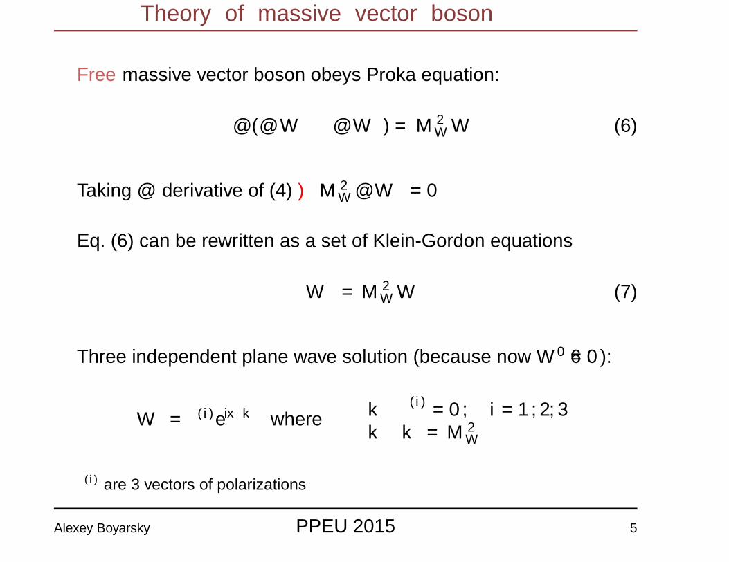
� Free massive vector boson obeys Proka equation:
∂ν(∂µW ν − ∂νWµ) = M2
WWµ (6)
� Taking ∂µ derivative of (4) ⇒M2W∂µW
µ = 0
� Eq. (6) can be rewritten as a set of Klein-Gordon equations
�Wµ = M2WW
µ (7)
� Three independent plane wave solution (because now W 0 6= 0):
Wµ = ε(i)µ eix·k where
{kµ · ε(i)µ = 0, i = 1, 2, 3kµ · kµ = M2
W
ε(i)µ are 3 vectors of polarizations
Alexey Boyarsky PPEU 2015 5
Theory of massive vector boson
� Consider W boson at rest
� The three polarization vectors are just three unit vectors along theaxes x, y, and z
� Now, make boost along z axis. W -bosons 4-momentum kµ =(E, 0, 0, kz)
� Three polarization vectors are
ε(1)µ (k) = (0, 1, 0, 0)
ε(2)µ (k) = (0, 0, 1, 0)
ε(3)µ (k) = 1
MW(kz, 0, 0, E)
� Consider W boson with energy E � MW , then kµ = (E, 0, 0, kz) ≈E(1, 0, 0, 1) when E ≈ kz �MW
Alexey Boyarsky PPEU 2015 6
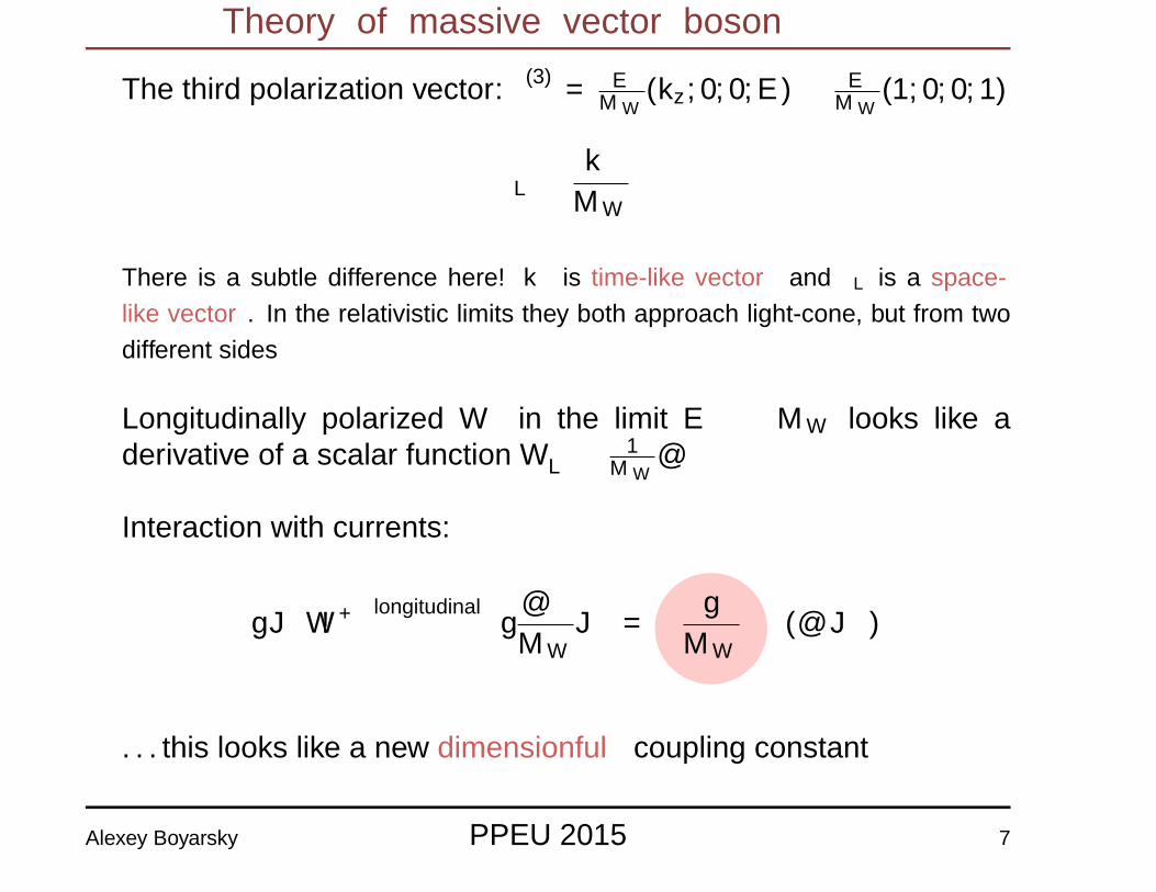
Theory of massive vector boson
� The third polarization vector: ε(3)µ = E
MW(kz, 0, 0, E) ≈ E
MW(1, 0, 0, 1)
εL ≈kµ
MW
� There is a subtle difference here! kµ is time-like vector and εL is a space-like vector. In the relativistic limits they both approach light-cone, but from twodifferent sides
� Longitudinally polarized Wµ in the limit E � MW looks like aderivative of a scalar function Wµ
L ≈1
MW∂µφ
� Interaction with currents:
gJ−µW+µ
longitudinal−−−−−−→ g∂µφ
MWJ−µ =
g
MWφ(∂µJ−µ )
� . . . this looks like a new dimensionful coupling constant
Alexey Boyarsky PPEU 2015 7
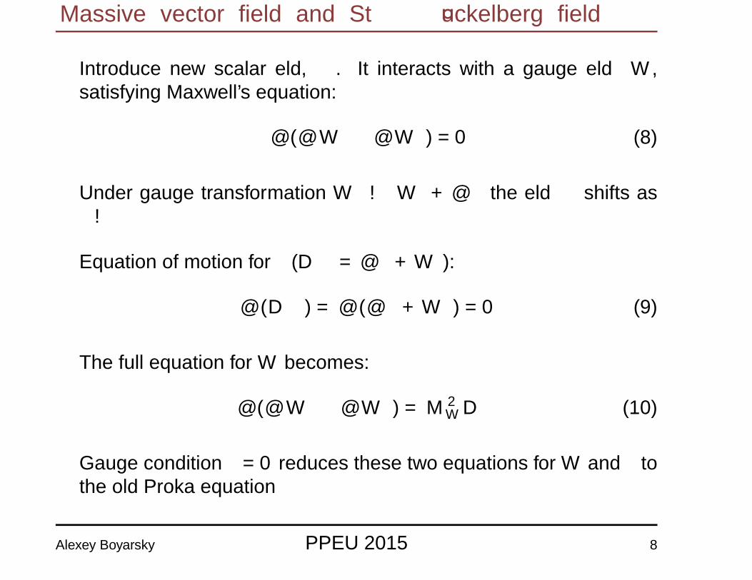
Massive vector field and Stuckelberg field
� Introduce new scalar field, θ. It interacts with a gauge field W ,satisfying Maxwell’s equation:
∂ν(∂µW ν − ∂νWµ) = 0 (8)
� Under gauge transformation Wµ → Wµ + ∂µλ the field θ shifts asθ → θ − λ
� Equation of motion for θ (Dµθ = ∂µθ +Wµ):
∂µ(Dµθ) = ∂µ(∂µθ +Wµ) = 0 (9)
� The full equation for W becomes:
∂ν(∂µW ν − ∂νWµ) = M2
WDµθ (10)
� Gauge condition θ = 0 reduces these two equations for W and θ tothe old Proka equation
Alexey Boyarsky PPEU 2015 8
Vector boson vs. photon
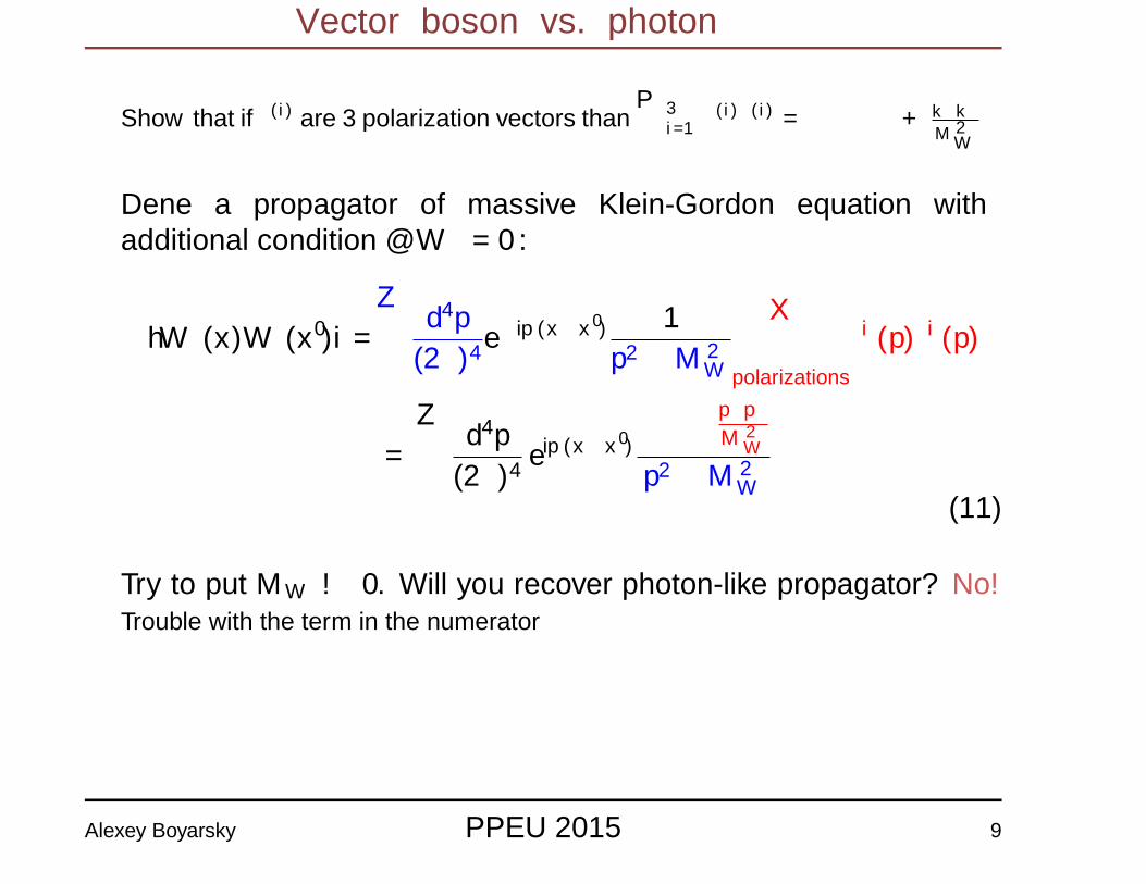
� Show that if ε(i)µ are 3 polarization vectors than
∑3i=1 ε
(i)µ ε
(i)ν =
(−ηµν + kµkν
M2W
)
� Define a propagator of massive Klein-Gordon equation withadditional condition ∂µWµ = 0:
〈Wµ(x)Wν(x′)〉 =
∫d4p
(2π)4e−ip(x−x
′) 1
p2 −M2W
∑polarizations
εiµ(p)εiν(p)
=
∫d4p
(2π)4eip(x−x
′)ηµν − pµpν
M2W
p2 −M2W
(11)
� Try to put MW → 0. Will you recover photon-like propagator? No!Trouble with the term in the numerator
Alexey Boyarsky PPEU 2015 9
Scattering eν → eν
� The relevant part of the interaction Lagrangian is
∆L = gW+µ
1√2νeγ
µPLe+ gW−µ1√2eγµPLνe (12)
PL = 12(1 − γ5) – projector of the 4-component spinor on the left
chirality.
� The relevant matrix element is given by
iM =
(ig√
2
)2
[u(k1)γµPLu(p2)] (−i)
gµν − rµrνM2W
r2 −M2W
[u(k2)γνPLu(p1)]
(13)
� After average over polarization of the colliding electron andsummation over polarizations of other particles we obtain:
¯|M|2 =g4s2
2(r2 −M2W )2
, s = (p1 + p2)2 (14)
Alexey Boyarsky PPEU 2015 10
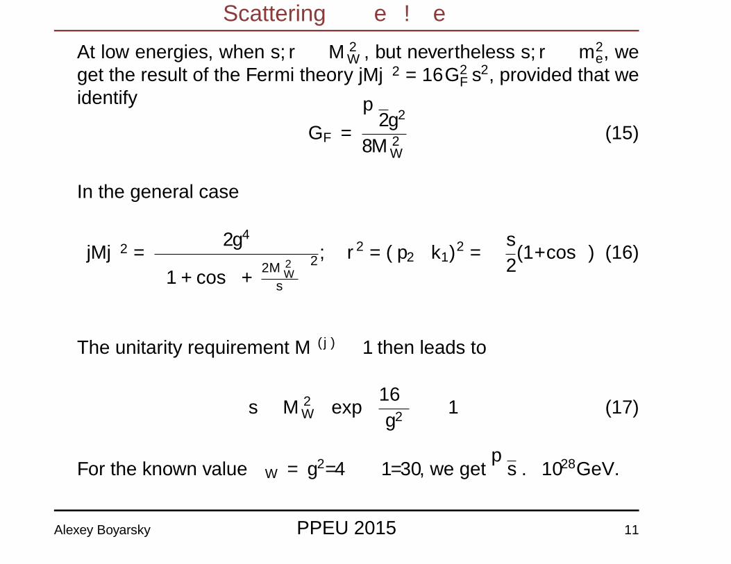
Scattering eν → eν
� At low energies, when s, r � M2W , but nevertheless s, r � m2
e, weget the result of the Fermi theory ¯|M|2 = 16G2
Fs2, provided that we
identify
GF =
√2g2
8M2W
(15)
� In the general case
¯|M|2 =2g4(
1 + cos θ +2M2
Ws
)2, r2 = (p2−k1)2 = −s2
(1+cos θ) (16)
� The unitarity requirementM(j) ≤ 1 then leads to
s ≤M2W
[exp
(16π
g2
)− 1
](17)
For the known value αW = g2/4π ≈ 1/30, we get√s . 1028GeV.
Alexey Boyarsky PPEU 2015 11
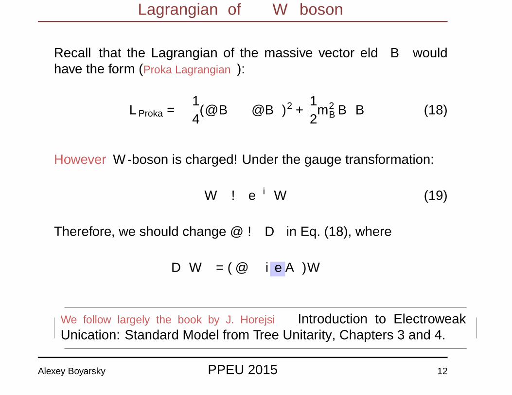
Lagrangian of W boson
� Recall that the Lagrangian of the massive vector field Bµ wouldhave the form (Proka Lagrangian):
LProka = −1
4(∂µBν − ∂νBµ)2 +
1
2m2BB
µBµ (18)
� However W -boson is charged! Under the gauge transformation:
W±µ → e±iαW±µ (19)
Therefore, we should change ∂µ → Dµ in Eq. (18), where
DµW±ν = (∂µ ± i e Aµ)W±ν
�
�
�
�We follow largely the book by J. Horejsi “Introduction to ElectroweakUnification: Standard Model from Tree Unitarity”, Chapters 3 and 4.
Alexey Boyarsky PPEU 2015 12
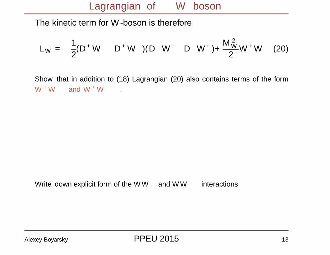
Lagrangian of W boson
� The kinetic term for W -boson is therefore
LW = −1
2(D+
µW−ν −D+
µW−ν )(D−µW
+ν −D−µW+
ν )+M2W
2W+µ W
−µ (20)
� Show that in addition to (18) Lagrangian (20) also contains terms of the formW+W−γ and W+W−γγ.
1
� Write down explicit form of the WWγ and WWγγ interactions
Alexey Boyarsky PPEU 2015 13
νeνe→W+W− scattering
1
� The amplitude of the process:
iM = v(p1)
(ig√
2γµPL
)i /q
q2
(ig√
2γνPL
)u(p2)ε
∗µ(k1)ε
∗ν(k2)
� Take s � m2e (so that mass of electron was neglected in the fermion
propagator).
¯|M|2 =∑s
|M|2 = (21)
=g2
4q2q2Tr[/p1 γ
µ/q γ
ν/p2 γ
ρ/q γ
λ](−gµλ +
k1µk1λ
M2W
)(−gνρ +
k2νk2ρ
M2W
)
� In the high-energy approximation s, q2 � MW dominateslongitudinal part, coming from k1,2/MW (i.e. one can neglect gµν term in
Alexey Boyarsky PPEU 2015 14
νeνe→W+W− scattering
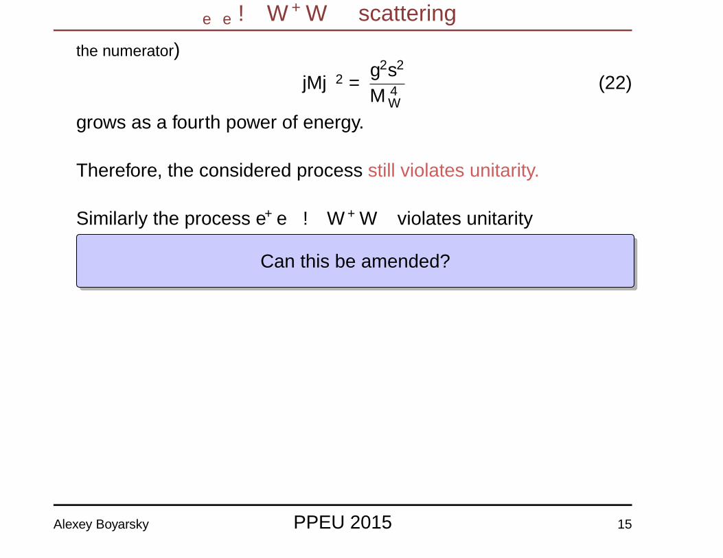
the numerator)¯|M|2 =
g2s2
M4W
(22)
grows as a fourth power of energy.
� Therefore, the considered process still violates unitarity.
� Similarly the process e+e− →W+W− violates unitarity
Can this be amended?
Alexey Boyarsky PPEU 2015 15
More contributions to ee→WW
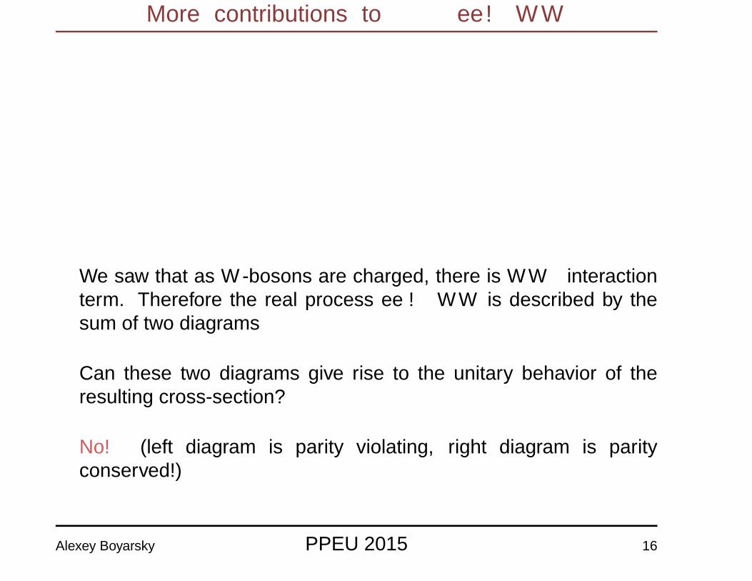
� We saw that as W -bosons are charged, there is WWγ interactionterm. Therefore the real process ee → WW is described by thesum of two diagrams
� Can these two diagrams give rise to the unitary behavior of theresulting cross-section?
� No! (left diagram is parity violating, right diagram is parityconserved!)
Alexey Boyarsky PPEU 2015 16
New particle is needed
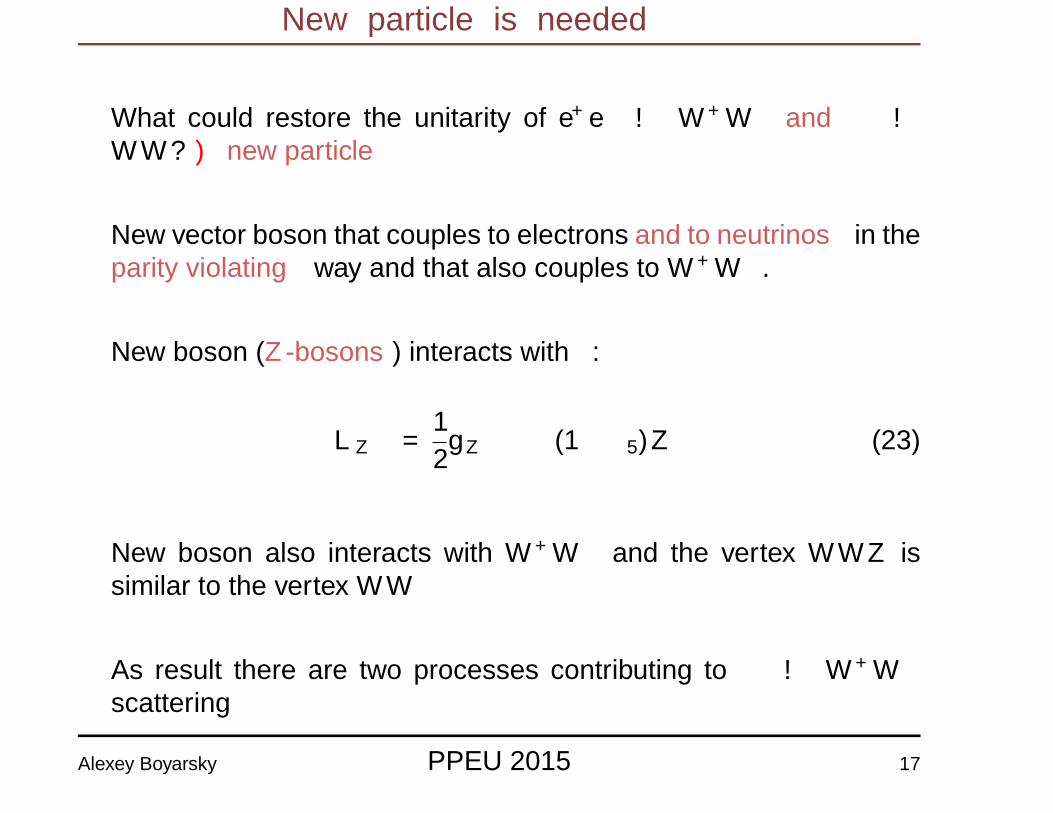
� What could restore the unitarity of e+e− → W+W− and νν →WW? ⇒new particle
� New vector boson that couples to electrons and to neutrinos in theparity violating way and that also couples to W+W−.
� New boson (Z-bosons) interacts with ν:
LννZ =1
2gννZνγ
µ(1− γ5)νZµ (23)
� New boson also interacts with W+W− and the vertex WWZ issimilar to the vertex WWγ
� As result there are two processes contributing to νν → W+W−
scattering
Alexey Boyarsky PPEU 2015 17
New particle is needed
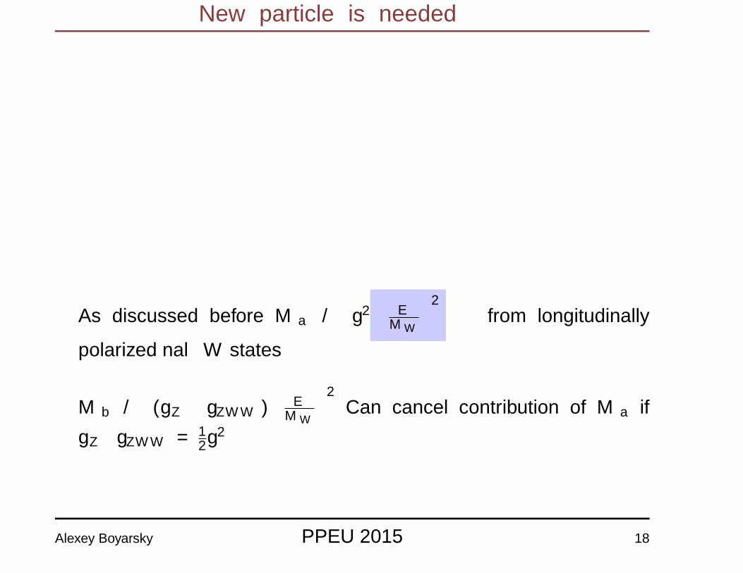
� As discussed before Ma ∝ g2(
EMW
)2
← from longitudinally
polarized final W states
� Mb ∝ (gννZ gZWW )(
EMW
)2
Can cancel contribution of Ma ifgννZgZWW = 1
2g2
Alexey Boyarsky PPEU 2015 18
Z-boson contribution to e+e−→W+W−
� Similarly, for e+e− →W+W− we would have three contributions tothe matrix element: |M|2 =
∣∣Ma +Mb + Mc
∣∣2
� Interaction with electrons:
Vint = gLeLγµeLZµ + gReRγ
µeRZµ (24)
Alexey Boyarsky PPEU 2015 19
New symmetry?
� Neutrino and electron – different charge. Different mass.
� . . . but! W -boson converts e→ νe or vice versa
� Neutron and proton – different charge. Different mass.
� . . . but! W -boson converts e→ νe or vice versa
� Wild guess:
Is there a new symmetry, that “rotates” e into νe(also µ into νµ, p into n, etc.)
Alexey Boyarsky PPEU 2015 20
Introduction to isospin
� Let we now have 2 different fermion fields ψ(1) and ψ(2) which arephysically equivalent for some interaction (good historical exampleis n and p for strong interactions).
� The Dirac equations are
(iγµ∂µ −m)ψ(1) + Vint(ψ(1)) =0 (25)
(iγµ∂µ −m)ψ(2) + Vint(ψ(2)) =0 (26)
� We can compose two-component field ~Ψ =
(ψ(1)
ψ(2)
)and rewrite the
Dirac equations using ~Ψ as
(iγµ∂µ −m) ~Ψ + Vint(~Ψ) = 0 (27)
Alexey Boyarsky PPEU 2015 21
Introduction to isospin
� Probability
P =
∫d3x
[ψ(1)γ0ψ(1) + ψ(2)γ0ψ(2)
]=
∫d3x ~Ψ+~Ψ
and Dirac equation (27) is invariant under global transformations:
~Ψ(x)→ ~Ψ′(x) = U~Ψ(x) (28)
that leaves the “length” of the two-dimensional isovector ~Ψinvariant.
� Such transformation is called unitary transformation and thematrix U in Eq. is 2 × 2 complex matrix which obeys conditionsU+U = 1 and det(U) = 1.
Alexey Boyarsky PPEU 2015 22
Yang-Mills: isospin ↔ vector field
EXCITATION FUNCTION OF C''(P, Pn) O'' REACTION
must then consider either the absolute value of theC"(p,pl) cross section or that of the AP7(p, 3prs) crosssection (or both) to be in error. We have rather arbi-trarily chosen to base our data on the 10.8-mb valuefor the AP'(p, 3prs) cross section at 420 Mev.Figure 1 shows that the cross section of the
C"(p,pcs) C" reaction is a fairly insensitive function ofthe energy of the incident proton in the energy rangestudied here. Since similar results were found for theproduction of Na", Na", and F" from aluminum andfor Be~ formation from carbon, 6 it appears to be gen-erally true that the probability of ejecting a smallnumber of nucleons from a small nucleus remains sub-stantially constant over a range of bombarding energiesfrom a few hundred Mev to at least 3 Bev. This impliesthat the probability that the incident particle leavesbehind a relatively small amount of energy (&100Mev)in the ieitia/ interaction with the nucleus is relativelyconstant over the wide energy range studied. Howeverwithin this energy range meson production increasesvery markedly with energy and becomes a probableprocess. If the nucleus is large these mesons would havea good chance of being reabsorbed in the nucleus inwhich they were produced. This would result in a shiftof the maximum in the total energy deposition spectrumto higher values, and reactions in which only a small'Hudis, Wolfgang, and Friedlander (unpublished).
40
Vl
lK
6)~ 20—X
10—
0.0I
0.5I
I.OI
l.58EV
I
2.0l
2.5I
3.0
Fro. 1. Excitation function of the C"(p,pn)C" reaction.
number of particles are ejected would become lesslikely. Such an eGect has been observed in our studieson heavier nuclei. ' However, in a small nucleus reab-sorption of mesons would be a much less importantmode of depositing excitation energy because of theirgreater escape probability. Thus it becomes plausiblethat while the increasing dominance of meson processesdecreases the cross sections for relatively simple reac-tions in heavy target nuclei, the cross sections for similarreactions of light nuclei remain almost unchanged.The help of the Cosmot. ron operating staff is grate-
fully acknowledged.
PH YSI CAL REVIEW VOLUME 96, NUMBER 1 OCTOB ER 1, 1954
Conservation of Isotopic Spin and Isotopic Gauge Invariance~C. N. YANG l' AND R. L. Mrr. r.s
Brookhaven SaHonal Laboratory, Upton, %em York(Received June 28, 1954)
It is pointed out that the usual principle of invariance under isotopic spin rotation is not consistant withthe concept of localized fields. The possibility is explored of having invariance under local isotopic spinrotations. This leads to formulating a principle of isotopic gauge invariance and the existence of a b Geldwhich has the same relation to the isotopic spin that the electromagnetic Geld has to the electric charge. Theb Geld satisGes nonlinear differential equations. The quanta of the b field are particles with spin unity,isotopic spin unity, and electric charge +e or zero.
INTRODUCTION
I 'HE conservation of isotopic spin is a much dis-cussed concept in recent years. Historically an
isotopic spin parameter was first. introduced by Heisen-berg' in 1932 to describe the two charge states (namelyneutron and. proton) of a nucleon. The idea that theneutron and proton correspond to two states of thesame particle was suggested at that time by the factthat their masses are nearly equal, and that the light*Work performed under the auspices of the U. S. Atomic
Energy Commission.t On leave of absence from the Institute for Advanced Study,
Princeton, New Jersey.' W. Heisenberg, Z. Physik 77, 1 (1932).
stable even nuclei contain equal numbers of them. Thenin 1937 Breit, Condon, and Present pointed out theapproximate equality of p—p and e—p interactions inthe 'S state. ' It seemed natural to assume that thisequality holds also in the other states available to boththe N—p and p—p systems. Under such an assumptionone arrives at the concept of a total isotopic spin' whichis conserved in nucleon-nucleon interactions. Experi-
'Breit, Condon, and Present, Phys. Rev. 50, 825 (1936). J.Schwinger pointed out that the small diAerence may be attributedto magnetic interactions /Phys. Rev. 78, 135 (1950)).
~ The total isotopic spin T was Grst introduced by E. Wigner,Phys. Rev. 51, 106 (1937); B. Cassen and E. U. Condon, Phys.Rev. 50, 846 (1936).
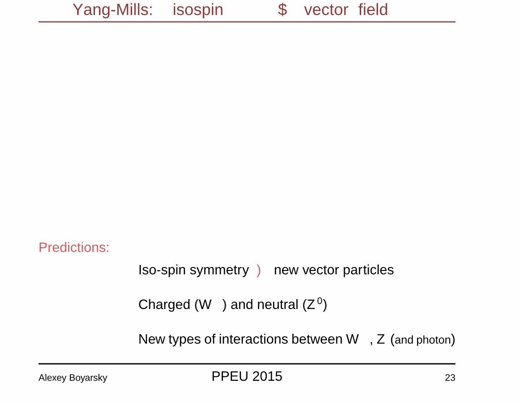
Predictions:
� Iso-spin symmetry ⇒ new vector particles
� Charged (W±) and neutral (Z0)
� New types of interactions between W±, Z (and photon)
Alexey Boyarsky PPEU 2015 23
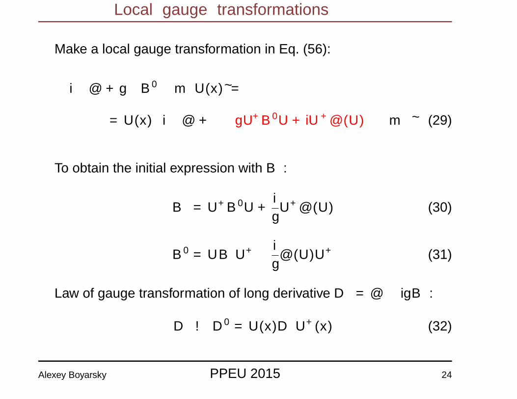
Local gauge transformations
� Make a local gauge transformation in Eq. (56):
(iγµ∂µ + gγµB′µ −m
)U(x)~Ψ =
= U(x)
(iγµ∂µ + γµ
(gU+B′µU + iU+∂µ(U)
)−m
)~Ψ (29)
� To obtain the initial expression with Bµ:
Bµ = U+B′µU +i
gU+∂µ(U) (30)
B′µ = UBµU+ − i
g∂µ(U)U+ (31)
� Law of gauge transformation of long derivative Dµ = ∂µ − igBµ:
Dµ → D′µ = U(x)DµU+(x) (32)
Alexey Boyarsky PPEU 2015 24
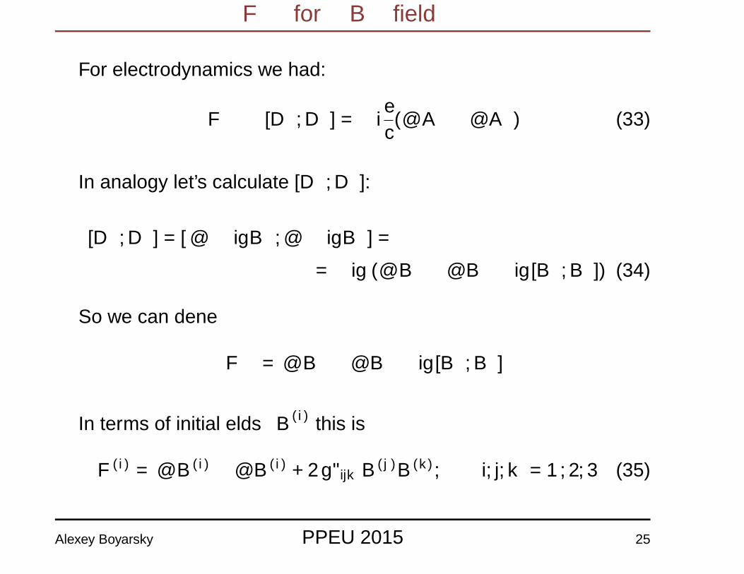
Fµν for Bµ field
� For electrodynamics we had:
Fµν ∼ [Dµ, Dν] = −iec(∂µAν − ∂νAµ) (33)
� In analogy let’s calculate [Dµ, Dν]:
[Dµ, Dν] = [∂µ − igBµ, ∂ν − igBν] =
= −ig (∂µBν − ∂νBµ − ig[Bµ, Bν]) (34)
So we can define
Fµν = ∂µBν − ∂νBµ − ig[Bµ, Bν]
� In terms of initial fields B(i)µ this is
F (i)µν = ∂µB
(i)ν − ∂νB(i)
µ + 2gεijkB(j)µ B(k)
ν , i, j, k = 1, 2, 3 (35)
Alexey Boyarsky PPEU 2015 25
Kinetic term for Bµ field
� From transformation law of long derivative Dµ → D′µ =U(x)DµU
+(x), so:
Fµν → F ′µν = U(x)FµνU+(x) (36)
� Notice the difference with electrodynamics. There Fµν was gaugeinvariant (electric and magnetic fields did not change when Aµ was gaugetransformed)
� Let us try to make a gauge-invariant term out of (36).
Tr(U(x)FµνU
+(x) U(x)FµνU+(x))
= Tr(FµνF
µν)
(37)
Recall that if you have any 3 matrices X,Y, Z, then Tr(X Y Z) =
Tr(Y Z X) = Tr(Z X Y )
Alexey Boyarsky PPEU 2015 26
Equations of motion
� Equations of motion for the field Bµ can be constructed as Euler-Lagrange equation for the action, starting from the gauge-invariantLagrangian
LB = −1
4Tr(FµνF
µν) = −1
4
3∑i=1
F (i)µνF
(i),µν (38)
� In terms of initial fields B(i)µ we can define:
F (i)µν = ∂µB
(i)ν − ∂νB(i)
µ + 2gεijkB(j)µ B(k)
ν (39)
Using this definition we can write Fµν = 2F(i)µν ti and:
From full Lagrangian we have:
∂µF(i),µν = J (i),ν − 2gεijkB
(j)µ F (k),µν (40)
where J (i),µ = igΨγµti~Ψ.
� We see, that even in the absence of matter fields B(i)µ are self-
interacting.
Alexey Boyarsky PPEU 2015 27
New types of interactions
� Charged nature of the W -bosons leads to two new interactionvertices involving photon
1
� We deduced some of them from (DµWν −DνWµ)2 kinetic term
� Yang-Mills theory predicts another gauge invariant terms,containing 2 W -bosons plus 1 photon or Z boson:
Lnon-minimal = eκFµνW+µ W
−ν (41)
where κ is a dimensionless constant.
Alexey Boyarsky PPEU 2015 28
New types of interactions
notice that the diagram (a) depends both minimal term e that has the structure ofeW∂WA and non-minimal term (41) of the form eκWW∂A
� The interaction vertex WWγ has the following form (for the choice ofmomentum as shown in Fig. (a) above)
Vλµν(k, p, q) =e (k − p)νηµλ + (p− q)ληµν + (q − k)µηνλ︸ ︷︷ ︸≡V YM
λµν(k,p,q)
+ e(1− κ)(qληµν − qµηνλ)
(42)
� The interaction vertex WWγγ has the structure independent on κ,but proportional on e2 rather than e.
Vµνρσ = − e2 (2ηµνηρσ − ηµρηνσ − ηµσηνρ) (43)
� Show that vertex V YMλµν(k, p, q) is symmetric with respect to cyclic change k →
p→ q with the simultaneous λ→ µ→ ν.
Alexey Boyarsky PPEU 2015 29
WW → γγ scattering
� The process W+ + W− → γ + γ has contribution from both WWγand WWγγ:
1
where the first two terms come from the WWγ vertex and the last one fromWWγγ.
� . . . keep in mind that the vertex WWγ depends on yet unknowncoefficient κ, entering Eqs. (41) and (42) (for example, κ = 0, i.e.“minimal coupling only” is allowed)
� Let us evaluate the high energy behavior of this process. Onecan expect that the largest contribution to the diagram comes fromthe term qµqν
M2W
1q2−M2
Win the propagator of the virtual W -boson in
diagrams (a) and (b).
Alexey Boyarsky PPEU 2015 30
WW → γγ scattering
� Working out the details (see Horejshi, Eqs. 4.20-4.23 and the text aroundthem) one can see that
�
�
�
�The process WW → γγ violates unitarity at high energiesunless κ = 1
� The same is true for the process γ +W → γ +W
� This special value of κ = 1 is exactly the one, predicted by theSU(2) gauge invariance!
Alexey Boyarsky PPEU 2015 31
Degrees of freedom and mass term
� For 3 massless fields B(i)µ we have 12 components, 3 independent
gauge transformations and 3 Gauss laws. So we have 6 degrees offreedom. We will associate those fields with W± and Z bosons.
� But every massless field we have to see at low energies. So ourfields have to be massive:
LB = −1
4
3∑i=1
F (i)µνF
(i),µν −M2i B
(i)µ B(i),µ
2(44)
� Mass term breaks gauge invariance and gives 3 new longitudinaldegrees of freedom.
Alexey Boyarsky PPEU 2015 32
Problems of mass term
� In formalism of Stuckelberg field we can rewrite longitudinaldegrees of freedom at high energies (E � Mi) using derivativesof scalar field θ:
B(i),Lµ ≈ 1
Mi∂µθ (45)
As we have B4 term in Lagrangian this means, that at high energieswe obtain dimensionful coupling constant and theory become nonrenormalizable.
� May be, as in electrodynamics, those degrees of freedom can’t beexcited? No! This field interact non only with conserved currentmade of fermions (where longitudinal degree of freedom can notbe excited, as J (i),µB
(i),Lµ = J (i),µ 1
Mi∂µθ = −∂µJ (i),µ 1
Miθ = 0
and ∂µJ(i),µ = 0), but also with gauge field contribution to current
(self interaction), which is not conserved and, therefore, longitudinalcomponent will be excited! It can not be avoided.
� What to do? How to describe massive vector fields then?
Alexey Boyarsky PPEU 2015 33
Massive vector bosons and gauge theories
� Electro-magnetic interactions of fermions are ”minimal” interactioni.e. they are required by local (space-time dependent) symmetry –gauge symmetry.
� Previously we have see that a self-content theory of weakinteractions can by made if these interactions are mediated by 3massive vector bosons, two charged (W± and one neutral (Z).
� Is there a symmetry which requires the existence of W± and Z?
� Triplet of intermediate bosons reminds the triplet ~Bµ of Y-M SU(2)fields that we discussed last time.
� However, our fields are massive and, therefore, gauge invariancewould be broken. Moreover, the theory of interacting massivevector fields is ill-defined, as longitudinal polarisation effectively hasdimension-full coupling constant and causes problems.
Alexey Boyarsky PPEU 2015 34
Spontaneous symmetry breaking
Alexey Boyarsky PPEU 2015 35
Spontaneous symmetry breaking
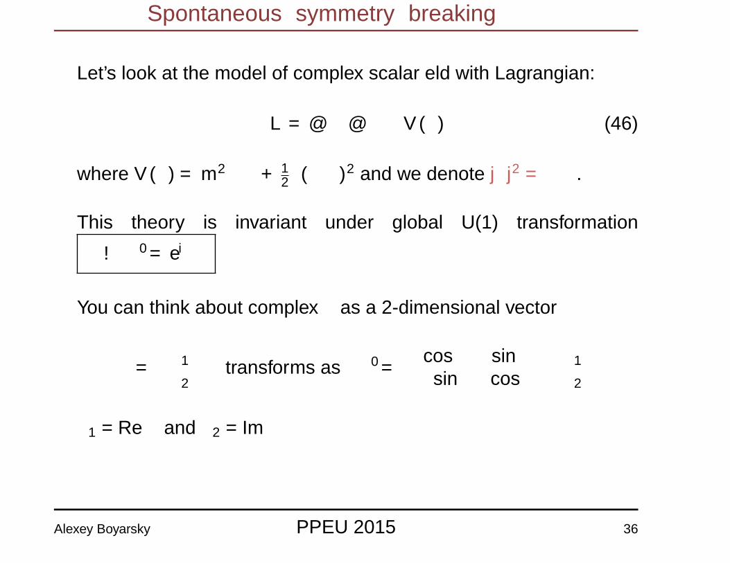
� Let’s look at the model of complex scalar field with Lagrangian:
L = ∂µφ∗∂µφ− V (φ) (46)
where V (φ) = m2φ∗φ+ 12λ(φ∗φ)2 and we denote |φ|2 = φ∗φ.
� This theory is invariant under global U(1) transformation
φ→ φ′ = eiαφ
� You can think about complex φ as a 2-dimensional vector
φ =
(φ1
φ2
)transforms as φ′ =
(cosα sinα− sinα cosα
)(φ1
φ2
)φ1 = Reφ and φ2 = Imφ
Alexey Boyarsky PPEU 2015 36
Spontaneous symmetry breaking
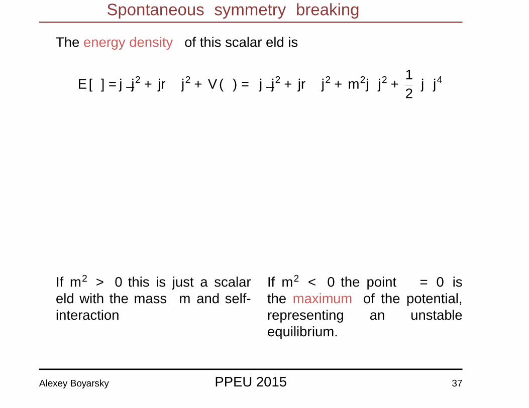
� The energy density of this scalar field is
E[φ] =|φ|2 + |∇φ|2 + V (φ) = |φ|2 + |∇φ|2 +m2|φ|2 +1
2λ|φ|4
If m2 > 0 this is just a scalarfield with the mass m and self-interaction λ
If m2 < 0 the point φ = 0 isthe maximum of the potential,representing an unstableequilibrium.
Alexey Boyarsky PPEU 2015 37
Spontaneous symmetry breaking
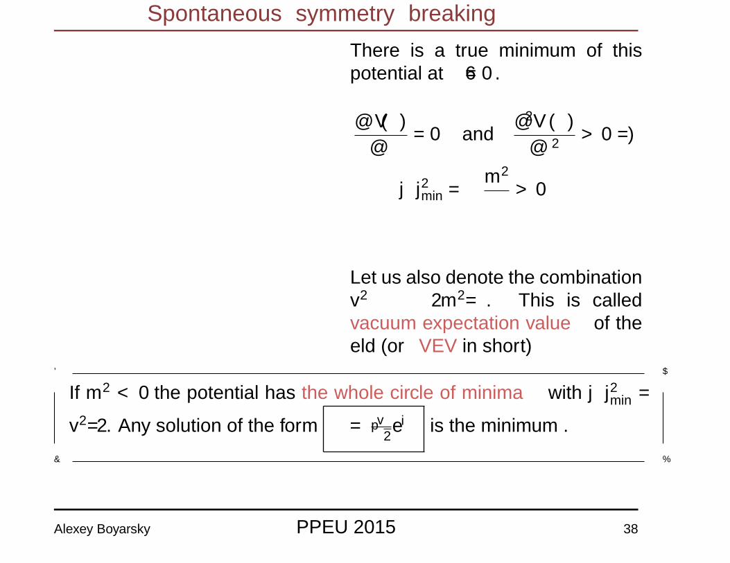
There is a true minimum of thispotential at φ 6= 0.
∂V (φ)
∂φ= 0 and
∂2V (φ)
∂φ2> 0 =⇒
|φ|2min = −m2
λ> 0
Let us also denote the combinationv2 ≡ −2m2/λ. This is calledvacuum expectation value of thefield (or VEV in short)
'
&
$
%
If m2 < 0 the potential has the whole circle of minima with |φ|2min =
v2/2. Any solution of the form φ = v√2eiθ is the minimum .
Alexey Boyarsky PPEU 2015 38
Spontaneous symmetry breaking
� Potential is invariant under U(1) transformation φ→ φ′ = eiαφ
� This transformation rotates one vacuum solution into another
φ =v√2eiθ −→ φ′ =
v√2ei(θ+α)
� Choosing a particular solution (for example, φmin = v√2
– real and positiveconfiguration) breaks the symmetry (it is not possible anymore applyφ′ = eiαφ transformation)
� However, does not change if instead we choose φmin = − v√2
orφmin = v√
2eiπ2
� The presence of the spontaneously broken symmetry in the systemmanifests itself in a special way – as a massless particle.
Alexey Boyarsky PPEU 2015 39
Goldstone boson
� Let us compute energy for the configuration φ(x) = v√2eiθ(x). This
is not a vacuum, as θ depends on x!
� The potential V (φ) depends only on |φ|, so V(v√2eiθ(x)
)= −m
4
2λ —independent on θ(x). Therefore
E
[φ(x) =
v√2eiθ(x)
]=v2
2
(θ2 + (∇θ)2
)− m
4
2λ
— energy of a free massless field with equation of motion �θ = 0
� This excitation is called Goldstone boson
� The massless field θ describes motion along the circle of minima inthe “Mexican hat potential”
Alexey Boyarsky PPEU 2015 40
Goldstone theorem
� Displace our solution from the minimum in the direction orthogonalto the circle:
φ(x) =v√2eiθ + δφ(x) =
1√2
(v + ρ(x)
)(47)
� The energy now has the form:
E[ρ] =1
2ρ2 +
1
2(∇ρ)2 +
1
2v2λρ2 + 1
2vλρ3 + λ
8ρ4 − λ
8v4
mass term for ρ self-interactions of ρ
� Oscillations in the direction perpendicular to the circle of vacua aredescribed by the massive real scalar field with the mass mρ = v
√λ
and equation of motion (�+m2ρ)ρ = 0
Alexey Boyarsky PPEU 2015 41
Spontaneous symmetry breaking
� The same result can be seen in a different way.
� Choose one particular minimum, say the one where field value isreal and positive (φ = v/
√2).
� The symmetry is now spontaneously broken – all minima areequivalent and you have chosen a particular one
� expanding about that point:
φ =1√2
(v + ϕ1 + iϕ2) (48)
where ϕi are two real scalar fields.
Alexey Boyarsky PPEU 2015 42
Spontaneous symmetry breaking
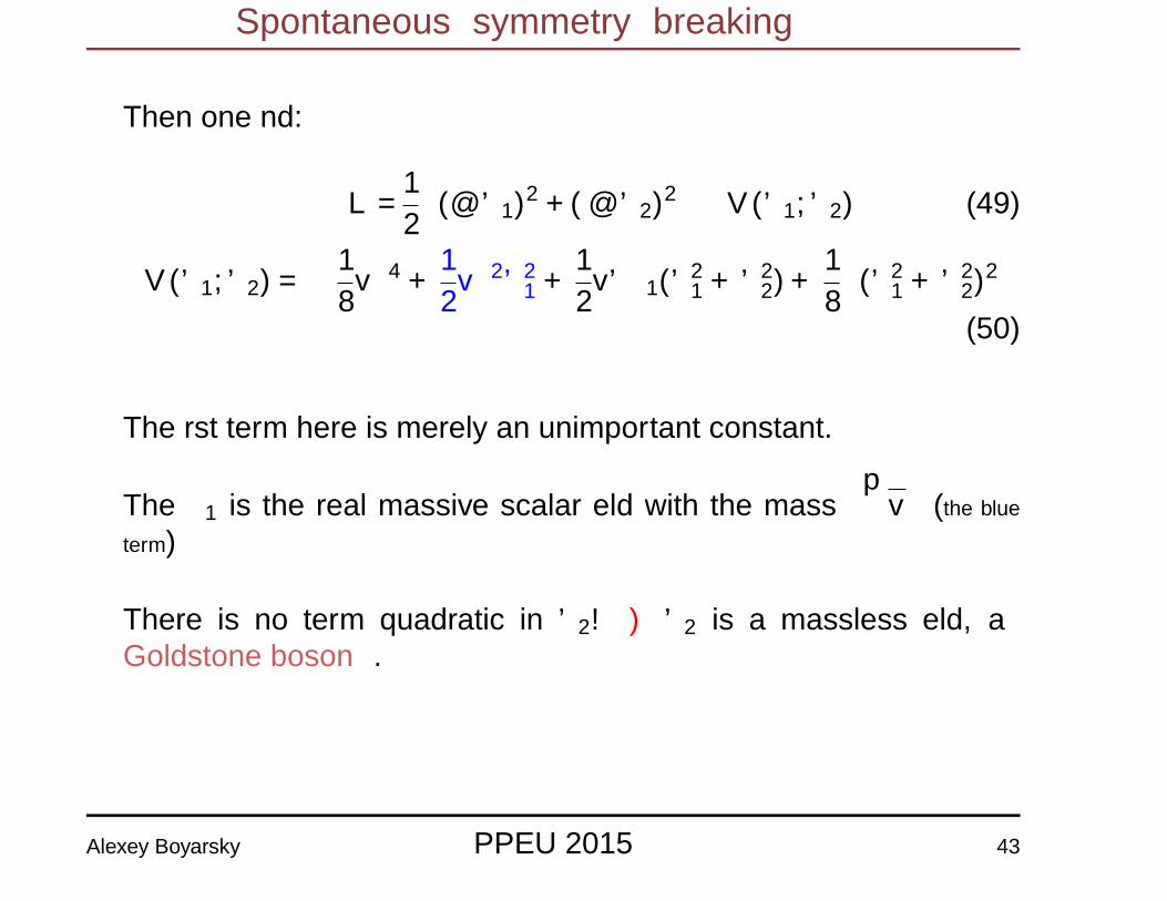
� Then one find:
L =1
2
[(∂µϕ1)2 + (∂µϕ2)2
]− V (ϕ1, ϕ2) (49)
V (ϕ1, ϕ2) = −1
8λv4 +
1
2λv2ϕ2
1 +1
2λvϕ1(ϕ2
1 + ϕ22) +
1
8λ(ϕ2
1 + ϕ22)2
(50)
� The first term here is merely an unimportant constant.
� The φ1 is the real massive scalar field with the mass√λv (the blue
term)
� There is no term quadratic in ϕ2! ⇒ϕ2 is a massless field, aGoldstone boson.
Alexey Boyarsky PPEU 2015 43
Higgs paper
Alexey Boyarsky PPEU 2015 44
Higgs vs. Stuckelberg models
� Models are similar to each other. Both have scalar field thatgenerate longitudinal components for vector fields and give themtheir masses.
� The main difference is that Higgs model has 2 fields and one ofthem stays massive. In general, we can write:
φ =1√2
(v + ϕ1 + iϕ2) = ρeiϕ (51)
Here ρ will be a massive field and ϕ is the full analogue of theStuckelberg field.
Alexey Boyarsky STRUCTURE OF THE STANDARD MODEL 45
WW →WW scattering
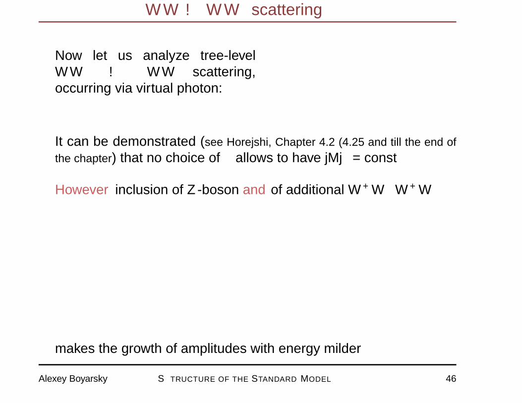
� Now let us analyze tree-levelWW → WW scattering,occurring via virtual photon:
1
� It can be demonstrated (see Horejshi, Chapter 4.2 (4.25 and till the end ofthe chapter) that no choice of κ allows to have |M| = const
� However inclusion of Z-boson and of additional W+W−W+W−
makes the growth of amplitudes with energy milder
Alexey Boyarsky STRUCTURE OF THE STANDARD MODEL 46
Higgs and Unitarity
e
�
e
+
W
+
W
�
e
�
e
+
W
+
W
�
Z
0
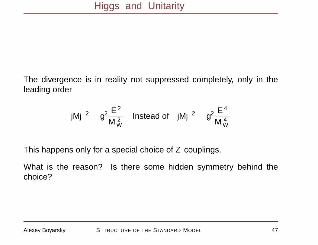
The divergence is in reality not suppressed completely, only in theleading order
|M|2 ∼ g2 E2
M2W
Instead of |M|2 ∼ g2 E4
M4W
This happens only for a special choice of Z couplings.
What is the reason? Is there some hidden symmetry behind thechoice?
Alexey Boyarsky STRUCTURE OF THE STANDARD MODEL 47
Higgs and Unitarity
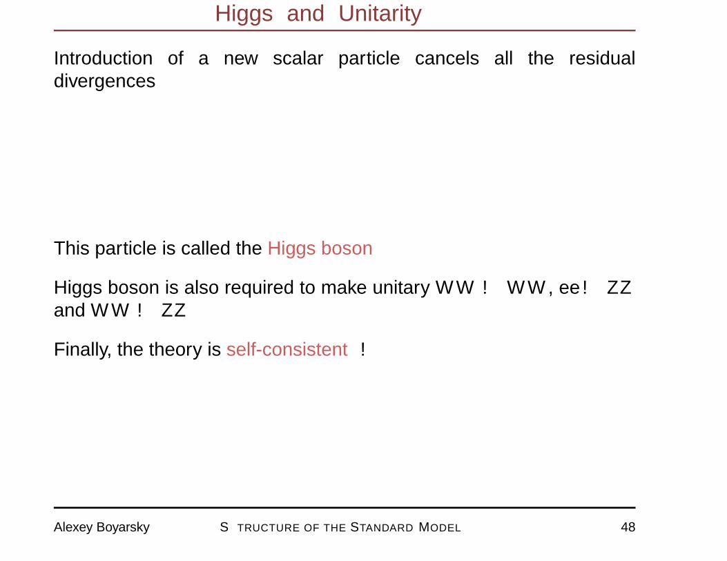
Introduction of a new scalar particle cancels all the residualdivergences
e
�
e
+
W
+
W
�
h
This particle is called the Higgs boson
Higgs boson is also required to make unitary WW → WW , ee→ ZZand WW → ZZ
Finally, the theory is self-consistent!
Alexey Boyarsky STRUCTURE OF THE STANDARD MODEL 48

Alexey Boyarsky STRUCTURE OF THE STANDARD MODEL 49
� Let us consider for simplicity only the theory containing thee, νe (as well γ and intermediate bosons W±, Z representingelectromagnetic and weak interactions).
� The symmetry that will be ”gauged” ( i.e. made space-timedependent) can then be a unitary transformation mixing wavefunctions of e and νe.
� Such a symmetry is U(2) symmetry, contacting 4 generators ( 3 forthe SU(2) part and one common phase for both fermions). Thisseems to be about right, as we need 4 vector bosons.
� However, e and νe have different massed and different electriccharges! The same is true for W± and Z. Also left and right leptonshave different charges under weak interactions
� Therefore, the symmetry should be broken. This would also help tomake vector bosons massive.
Alexey Boyarsky STRUCTURE OF THE STANDARD MODEL 50
Alexey Boyarsky STRUCTURE OF THE STANDARD MODEL 51
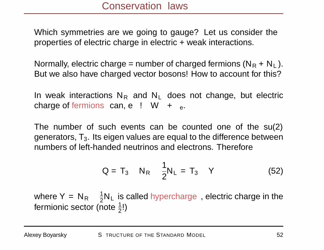
Conservation laws
� Which symmetries are we going to ”gauge”? Let us consider theproperties of electric charge in electric + weak interactions.
� Normally, electric charge = number of charged fermions (NR+NL).But we also have charged vector bosons! How to account for this?
� In weak interactions NR and NL does not change, but electriccharge of fermions can, e± →W± + νe.
� The number of such events can be counted one of the su(2)generators, T3. Its eigen values are equal to the difference betweennumbers of left-handed neutrinos and electrons. Therefore
Q = T3 −NR −1
2NL = T3 − Y (52)
where Y = NR− 12NL is called hypercharge, electric charge in the
fermionic sector (note 12!)
Alexey Boyarsky STRUCTURE OF THE STANDARD MODEL 52
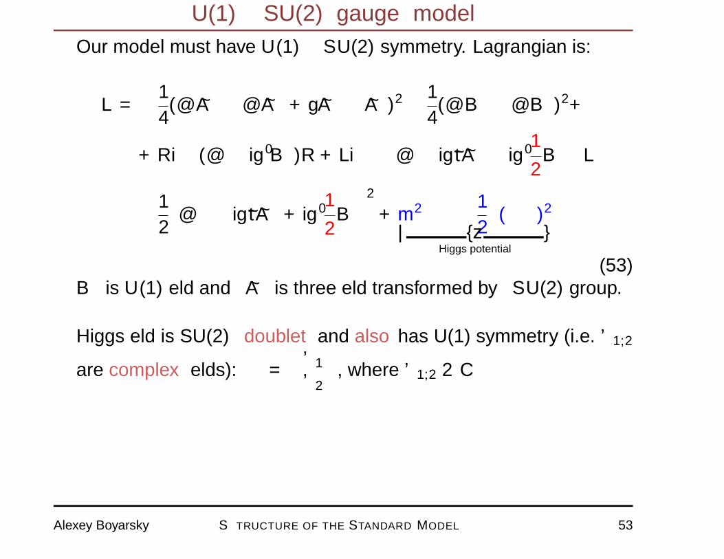
U(1)×SU(2) gauge model
� Our model must have U(1)× SU(2) symmetry. Lagrangian is:
L =− 1
4(∂µ ~Aν − ∂ν ~Aµ + g ~Aµ × ~Aν)
2 − 1
4(∂µBν − ∂νBµ)2+
+ Riγµ(∂µ − ig′Bµ)R+ Liγµ(∂µ − ig~t ~Aµ − ig′
1
2Bµ
)L−
− 1
2
∣∣∣∣∂µφ− ig~t ~Aµ + ig′1
2Bµ
∣∣∣∣2 +m2φ∗φ− 1
2λ(φ∗φ)2︸ ︷︷ ︸
Higgs potential
(53)Bµ is U(1) field and ~Aµ is three field transformed by SU(2) group.
� Higgs field is SU(2) doublet and also has U(1) symmetry (i.e. ϕ1,2
are complex fields): φ =
(ϕ1
ϕ2
), where ϕ1,2 ∈ C
Alexey Boyarsky STRUCTURE OF THE STANDARD MODEL 53
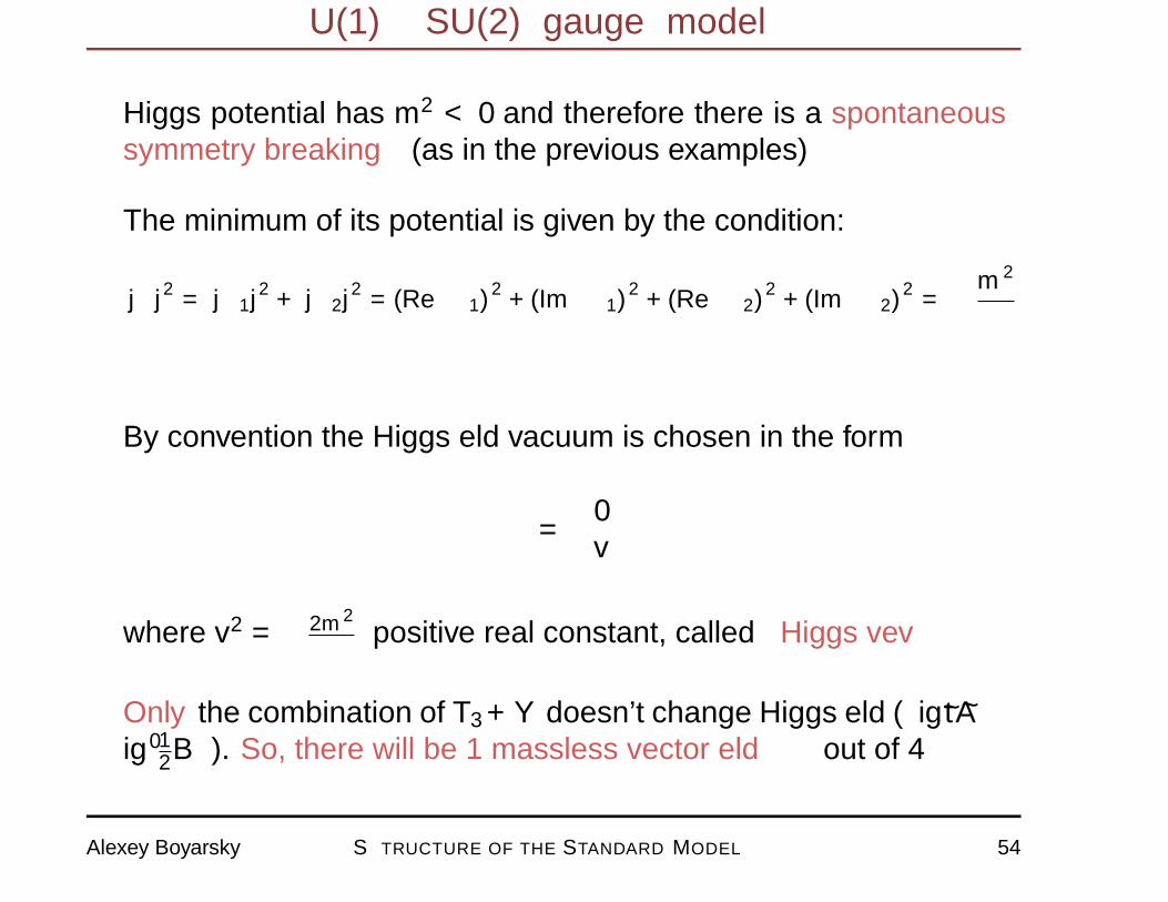
U(1)×SU(2) gauge model
� Higgs potential has m2 < 0 and therefore there is a spontaneoussymmetry breaking (as in the previous examples)
� The minimum of its potential is given by the condition:
|φ|2 = |φ1|2 + |φ2|2 = (Reφ1)2
+ (Imφ1)2
+ (Reφ2)2
+ (Imφ2)2
= −m2
λ
� By convention the Higgs field vacuum is chosen in the form
φ =
(0v
)
where v2 = −2m2
λ – positive real constant, called Higgs vev
� Only the combination of T3 +Y doesn’t change Higgs field (ig~t ~Aµ−ig′12Bµ). So, there will be 1 massless vector field out of 4
Alexey Boyarsky STRUCTURE OF THE STANDARD MODEL 54
Physical vector fields
� In our model physical observable will be combinations of Bµ and~Aµ fields:
W±µ =1√2
(A(1)µ ∓ iA(2)
µ
)(54)
Zµ =1√
g2 + g′2
(gA(3)
µ + g′Bµ
)(55)
Aµ =1√
g2 + g′2
(−g′A(3)
µ + gBµ
)(56)
� Masses of these fields areMW = 12gλ,MA = 0,MZ = 1
2
√g2 + g′2λ.
Also we can find electric charge as e = gg′/√g2 + g′2. The Fermi
constant in this terms is:
GF√2
=g2
8M2Z
=1
2λ2(57)
So we know λ value from GF . From measuring MW and e we’llfind g and g′. So we can predict MZ and make an independentexperimental cross-check.
Alexey Boyarsky STRUCTURE OF THE STANDARD MODEL 55
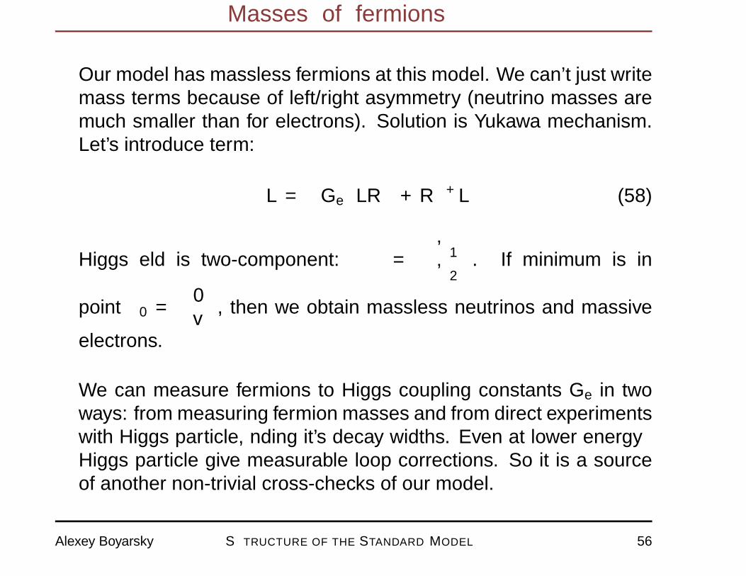
Masses of fermions
� Our model has massless fermions at this model. We can’t just writemass terms because of left/right asymmetry (neutrino masses aremuch smaller than for electrons). Solution is Yukawa mechanism.Let’s introduce term:
∆L = −Ge(LφR+ Rφ+L
)(58)
Higgs field is two-component: φ =
(ϕ1
ϕ2
). If minimum is in
point φ0 =
(0v
), then we obtain massless neutrinos and massive
electrons.
� We can measure fermions to Higgs coupling constants Ge in twoways: from measuring fermion masses and from direct experimentswith Higgs particle, finding it’s decay widths. Even at lower energyHiggs particle give measurable loop corrections. So it is a sourceof another non-trivial cross-checks of our model.
Alexey Boyarsky STRUCTURE OF THE STANDARD MODEL 56
Additional information
Alexey Boyarsky STRUCTURE OF THE STANDARD MODEL 57
Groups and algebras
Alexey Boyarsky STRUCTURE OF THE STANDARD MODEL 58
Groups
� Let matrices U1, U2 are such that U+i Ui = 1 and det(Ui) = 1. It’s
easy to see, that matrix U1U2 has this properties:
(U1U2)+U1U2 = U+2 U
+1 U1U2 =U+
2
(U+
1 U1
)U2 = U+
2 U2 = 1 (59)
det(U1U2) = det(U1) det(U2) = 1 (60)
Besides that, indentity matrix 1 and U−1i = U+
i also obey thisproperties.
Notice, that for example, U1 + U2 is in general not a unitary matrix. Also if U has detU = 1,
the matrix α× U has det(αU) = αn 6= 1
� This means that set of such matrices is closed under multiplicationand inversion operations and has unity element. In math such setscalled groups, in particular, this group has it’s own name — SU(2)group.
� The general element of SU(2) group is parametrized by three real
Alexey Boyarsky STRUCTURE OF THE STANDARD MODEL 59
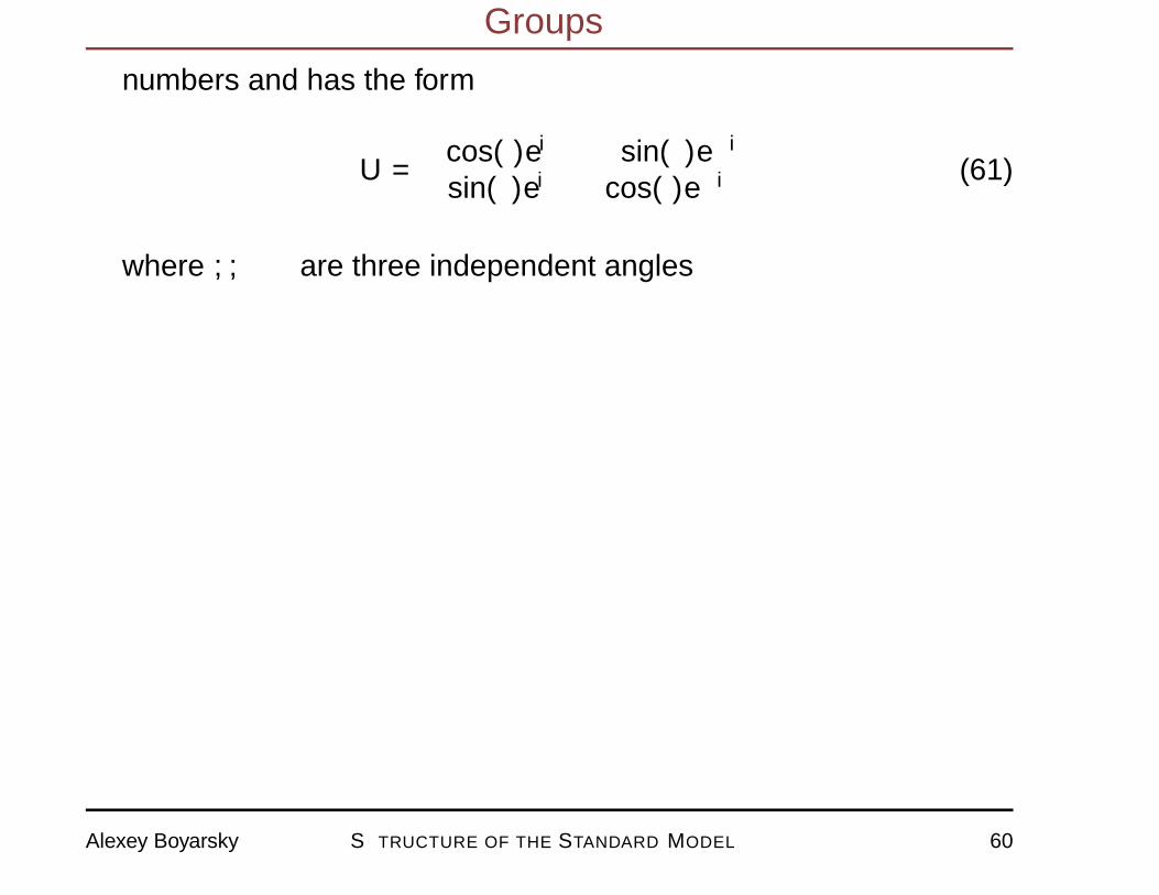
Groups
numbers and has the form
U =
(cos(θ)eiφ − sin(θ)e−iβ
sin(θ)eiβ cos(θ)e−iφ
)(61)
where θ, β, φ are three independent angles
Alexey Boyarsky STRUCTURE OF THE STANDARD MODEL 60
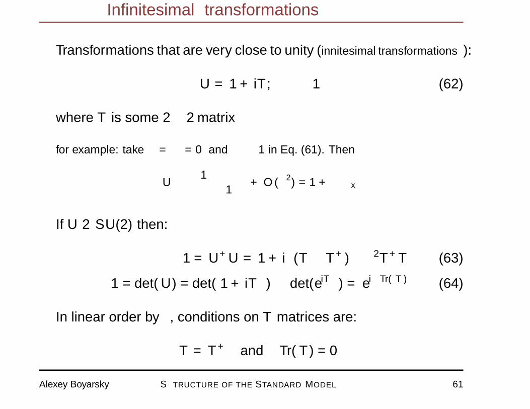
Infinitesimal transformations
� Transformations that are very close to unity (infinitesimal transformations):
U = 1+ iδT, δ � 1 (62)
where T is some 2× 2 matrix
� for example: take β = φ = 0 and θ � 1 in Eq. (61). Then
U ≈(
1 −θθ 1
)+O(θ
2) = 1 + θσx
� If U ∈ SU(2) then:
1 = U+U = 1+ iδ(T − T+)− δ2T+T (63)
1 = det(U) = det(1+ iδT ) ≈ det(eiδT ) = eiδTr(T ) (64)
In linear order by δ, conditions on T matrices are:
T = T+ and Tr(T ) = 0
Alexey Boyarsky STRUCTURE OF THE STANDARD MODEL 61
Infinitesimal transformations��
� Set of such matrices is called Hermitian
An example of Hermitian matrices are Pauli matrices (σx, σy, σz)
Alexey Boyarsky STRUCTURE OF THE STANDARD MODEL 62
SU(2)
Alexey Boyarsky STRUCTURE OF THE STANDARD MODEL 63
SU(2) algebra
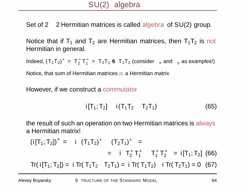
� Set of 2× 2 Hermitian matrices is called algebra of SU(2) group.
� Notice that if T1 and T2 are Hermitian matrices, then T1T2 is notHermitian in general.
Indeed, (T1T2)+ = T+
2 T+1 = T2T1 6= T1T2 (consider σx and σy as examples!)
Notice, that sum of Hermitian matrices is a Hermitian matrix
� However, if we construct a commutator
i[T1, T2] ≡ i(T1T2 − T2T1) (65)
the result of such an operation on two Hermitian matrices is alwaysa Hermitian matrix!
(i[T1, T2])+
= −i((T1T2)+ − (T2T1)+
)=
= −i(T+
2 T+1 − T
+1 T
+2
)= i[T1, T2] (66)
Tr(i[T1, T2]) = iTr(T1T2−T2T1) = iTr(T1T2)−iTr(T2T1) = 0 (67)
Alexey Boyarsky STRUCTURE OF THE STANDARD MODEL 64
SU(2) algebra
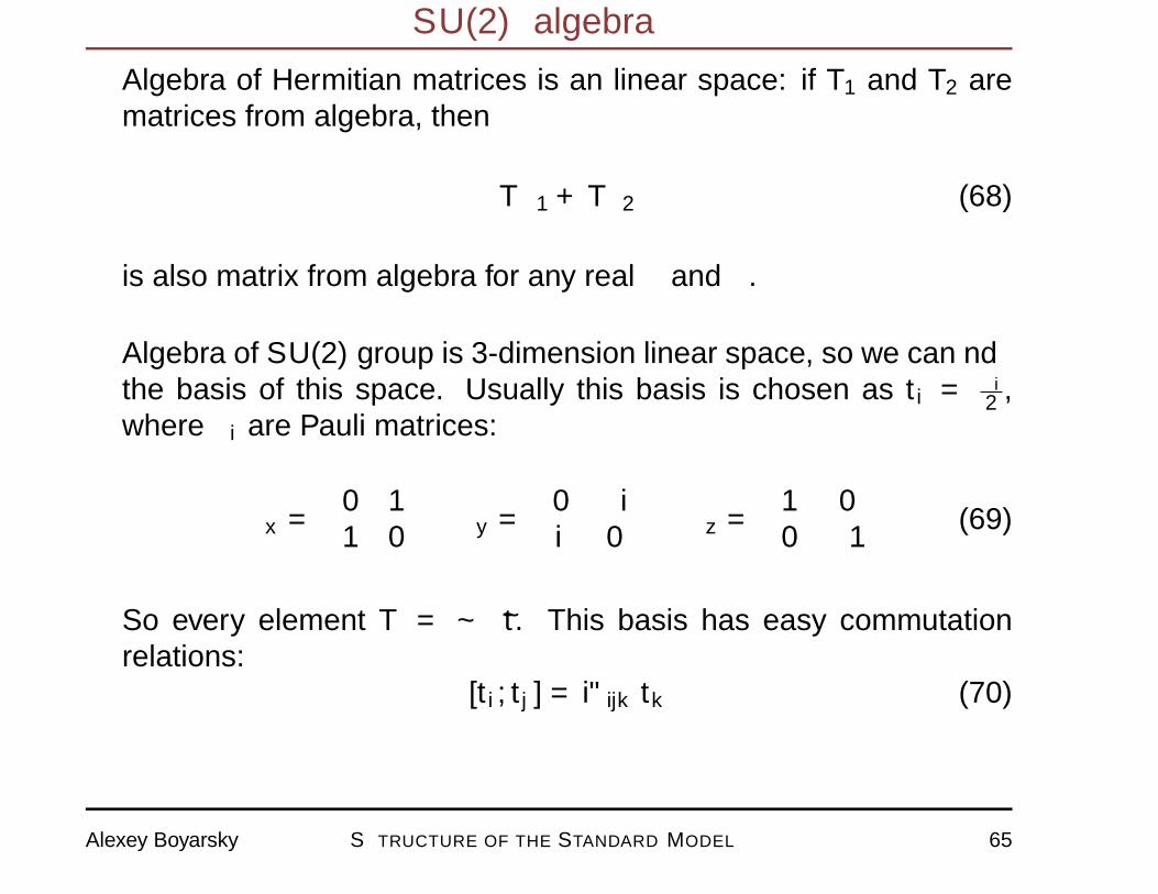
� Algebra of Hermitian matrices is an linear space: if T1 and T2 arematrices from algebra, then
αT1 + βT2 (68)
is also matrix from algebra for any real α and β.
� Algebra of SU(2) group is 3-dimension linear space, so we can findthe basis of this space. Usually this basis is chosen as ti = σi
2 ,where σi are Pauli matrices:
σx =
(0 11 0
)σy =
(0 −ii 0
)σz =
(1 00 −1
)(69)
So every element T = ~α · ~t. This basis has easy commutationrelations:
[ti, tj] = iεijktk (70)
Alexey Boyarsky STRUCTURE OF THE STANDARD MODEL 65
Exponential formula
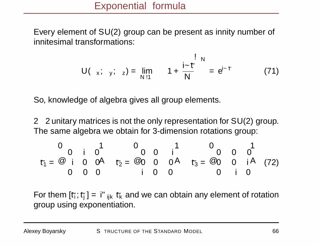
� Every element of SU(2) group can be present as infinity number ofinfinitesimal transformations:
U(αx, αy, αz) = limN→∞
(1+
i~α~t
N
)N= ei~α
~t (71)
So, knowledge of algebra gives all group elements.
� 2×2 unitary matrices is not the only representation for SU(2) group.The same algebra we obtain for 3-dimension rotations group:
t1 =
0 i 0−i 0 00 0 0
t2 =
0 0 −i0 0 0i 0 0
t3 =
0 0 00 0 i0 −i 0
(72)
For them [ti, tj] = iεijktk and we can obtain any element of rotationgroup using exponentiation.
Alexey Boyarsky STRUCTURE OF THE STANDARD MODEL 66
Local SU(2) transformations
� We saw that probability and other observables do not change if weinterchange two fermions ψ(1) and ψ(2).
� Can we make the SU(2) transformation local (i.e. ~Ψ′ → U(x)~Ψ)?
� We can write U(x) = ei(~α(x)~t) and after local transformation ~Ψ(x)→~Ψ′(x) = U(x)~Ψ(x) we have:
U(x)(iγµ∂µ − γµ∂µ(~α(x))~t−m
)~Ψ = 0 (73)
� As we have 3 independent functions αi(x) we need at least 3 fieldsto make the Equation (73) invariant.
� In analogy to QED we introduce 3 vector fields, B(1)µ , B(2)
µ and B(3)µ .
The main innovation is the way in which these fields interact:
Vint = gΨγµB(i)µ ti~Ψ =
=g
2
(ψ(1) ψ(2)
)γµ
(B
(3)µ B
(1)µ − iB(2)
µ
B(1)µ + iB
(2)µ −B(3)
µ
)(ψ(1)
ψ(2)
)(74)
Alexey Boyarsky STRUCTURE OF THE STANDARD MODEL 67
Local SU(2) transformations
� We obtain new Dirac equation
(iγµ∂µ + gγµBµ −m) Ψ = 0 (75)
where Bµ is a 2× 2 matrix Bµ =3∑i=1
B(i)µ ti.
Alexey Boyarsky STRUCTURE OF THE STANDARD MODEL 68
Reminder: local symmetries and gauge field
Alexey Boyarsky STRUCTURE OF THE STANDARD MODEL 69
Reminder: Appearance of EM field
� How Aµ field appeared in electrodynamics? Let’s look at the Diracequation:
(iγµ∂µ −m)ψ = 0 (76)
� This equation is invariant under global transformationψ(x)→ ψ′(x) = eiαψ(x).
� All physical observables (such as probability ψ†ψ or currentψγµψ) are invariant for such a transformation
� If we demand local gauge invariance ψ(x) → ψ′(x) = eiα(x)ψ(x),the probability, current, etc. still remain invariant.
Alexey Boyarsky STRUCTURE OF THE STANDARD MODEL 70
Reminder: Appearance of EM field
� However, the Dirac equation changes:
(iγµ∂µ −m)ψ′ =
= (iγµ∂µ −m) eiα(x)ψ =
= eiα(x) (iγµ∂µ − γµ(∂µα(x))−m)ψ (77)
� How to make this theory gauge invariant?
� Let’s introduce a new field. It couldn’t be fermionic field, cause wecan’t take 3-fermion and 4-fermion interaction (3-fermion interactiondoesn’t even exist and both would be higher than 4-dimensionoperators).
� Coupling with one scalar field we also can’t organize: minimalpossible interaction term gψγµψ∂µφ has dimension 5.
� So the last possibility is a coupling with some vector field. Theinteraction now becomes V = ψγµψAµ with some constant g. The
Alexey Boyarsky STRUCTURE OF THE STANDARD MODEL 71
Reminder: Appearance of EM field
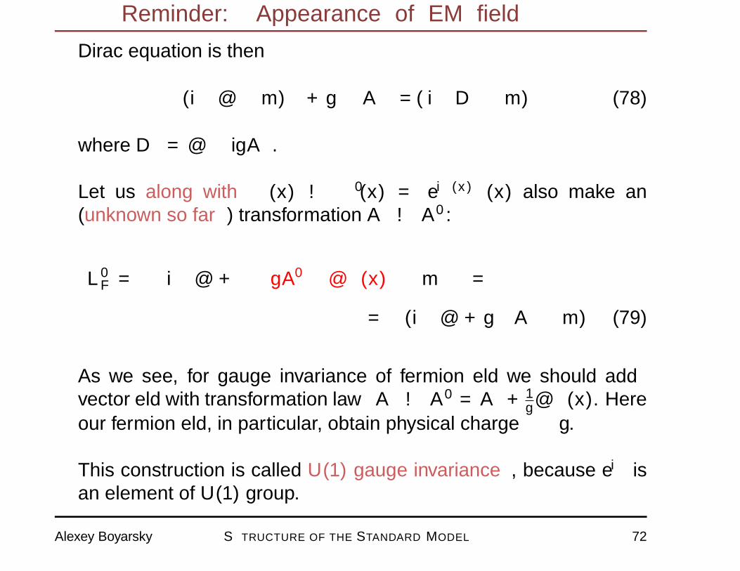
Dirac equation is then
(iγµ∂µ −m)ψ + gγµψAµ = (iγµDµ −m)ψ (78)
where Dµ = ∂µ − igAµ.
� Let us along with ψ(x) → ψ′(x) = eiα(x)ψ(x) also make an(unknown so far) transformation Aµ → A′µ:
L′F = ψ(iγµ∂µ + γµ
(gA′µ − ∂µα(x)
)−m
)ψ =
= ψ (iγµ∂µ + gγµAµ −m)ψ (79)
� As we see, for gauge invariance of fermion field we should addvector field with transformation law Aµ → A′µ = Aµ+ 1
g∂µα(x). Hereour fermion field, in particular, obtain physical charge — g.
� This construction is called U(1) gauge invariance, because eiα isan element of U(1) group.
Alexey Boyarsky STRUCTURE OF THE STANDARD MODEL 72
Reminder: Appearance of EM field
� If we’ve measured that vector field is massless, the only possibilityis to write the full theory is QED Lagrangian:
LQED = ψ (iγµDµ −m)ψ − 1
4FµνF
µν (80)
Alexey Boyarsky STRUCTURE OF THE STANDARD MODEL 73


![NONDECELERATIVE UNIVERSE MODEL - viXra · NONDECELERATIVE UNIVERSE 1: CHARACTERISTICS Our model of the Universe (Expansive Nondecelerative Universe, ENU) [1],[2],[3], is based on](https://img.pdfslide.tips/doc/110x75/5f1ebd7d98cc3b45d95e5387/nondecelerative-universe-model-vixra-nondecelerative-universe-1-characteristics.jpg)