Embed Size (px)
Citation preview
7/21/2019 PEER807 KRAMERArduino Shin
http://slidepdf.com/reader/full/peer807-kramerarduino-shin 1/198
PACIFIC EARTHQUAKE ENGINEERINGRESEARCH CENTER
PEER 2008/07 OVEMBER 2008
Using OpenSees for Performance-Based Evaluation of
Bridges on Liquefable Soils
Steven L. KramerUniversity of Washington
Pedro Arduino
University of Washington
HyungSuk Shin
Kleinfelder, Inc.
Seattle, Washington
7/21/2019 PEER807 KRAMERArduino Shin
http://slidepdf.com/reader/full/peer807-kramerarduino-shin 2/198
Using OpenSees for Performance-Based Evaluation of
Bridges on Liquefiable Soils
Steven L. Kramer
Department of Civil and Environmental EngineeringUniversity of Washington, Seattle
Pedro Arduino
Department of Civil and Environmental EngineeringUniversity of Washington, Seattle
HyungSuk Shin
Kleinfelder, Inc., Seattle
PEER Report 2008/07Pacific Earthquake Engineering Research Center
College of EngineeringUniversity of California, Berkeley
November 2008
7/21/2019 PEER807 KRAMERArduino Shin
http://slidepdf.com/reader/full/peer807-kramerarduino-shin 3/198
iii
ABSTRACT
By virtue of their locations, bridges that cross bodies of water are particularly likely to be
damaged by lateral spreading of liquefied soils. The behavior of these soils can cause unusualforms of seismic demands on bridges and their foundations, ranging from rapid modifications of
input motion amplitudes and frequency contents to high levels of kinematic loading associated
with permanent deformations of the supporting soils. This report describes the application of the
PEER methodology of performance-based earthquake engineering to a bridge structure founded
on liquefiable soils. In this investigation, the response of the soil-foundation-structure system
was computed using detailed nonlinear inelastic analyses. The computer program, OpenSees,
was used to model liquefiable and non-liquefiable soils, pile foundations, abutments, and the
bridge superstructure. The detailed model enabled direct prediction of the response of critical
bridge elements, hence the more accurate estimation of resulting physical damage and loss. The
report presents a detailed description of the site, the analytical model and its validation, the
computed response under various loading conditions, and the resulting damage and loss
estimates. The response and losses under conditions where the bridge is supported on non-
liquefiable soils and on rock are also computed and compared with the liquefaction case.

7/21/2019 PEER807 KRAMERArduino Shin
http://slidepdf.com/reader/full/peer807-kramerarduino-shin 4/198
iv
ACKNOWLEDGMENTS
This work was supported primarily by the Earthquake Engineering Research Centers Program of
the National Science Foundation under award number EEC-9701568 through the PacificEarthquake Engineering Research (PEER) Center. Any opinions, findings, and conclusions or
recommendations expressed in this material are those of the author(s) and do not necessarily
reflect those of the National Science Foundation.
7/21/2019 PEER807 KRAMERArduino Shin
http://slidepdf.com/reader/full/peer807-kramerarduino-shin 5/198
v
CONTENTS
ABSTRACT .................................................................................................................................. iii
ACKNOWLEDGMENTS ........................................................................................................... iv TABLE OF CONTENTS............................................................................................................. v
LIST OF FIGURES ..................................................................................................................... xi
LIST OF TABLES .................................................................................................................... xvii
1 INTRODUCTION ................................................................................................................ 1
1.1. Background .................................................................................................................... 1
1.2. Performance-Based Earthquake Engineering................................................................. 2
1.3. Objectives of the Study .................................................................................................. 3
1.4. Organization ................................................................................................................... 3
2 PERFORMANCE-BASED EARTHQUAKE ENGINEERING....................................... 5
2.1 Introduction .................................................................................................................... 5
2.2 PEER Framework........................................................................................................... 5
2.3 Response Prediction ....................................................................................................... 7
2.4 Damage Prediction ......................................................................................................... 8
2.5 Loss Prediction ............................................................................................................... 9
2.6 Summary ........................................................................................................................ 9
3 SEISMIC SOIL-PILE-STRUCTURE INTERACTION................................................. 11
3.1 Introduction .................................................................................................................. 11
3.2 Soil-Pile Interaction Modeling..................................................................................... 11
3.2.1 Static and Dynamic Beam-on-Nonlinear-Winkler-Foundation (BNWF)
Models.............................................................................................................. 12
3.3 P-y Curves .................................................................................................................... 13
3.3.1 Conventional p-y Curves for Piles Subjected to Static and Cyclic Loading..... 13
3.3.1.1 Back-Calculated p-y Curves for Sand, Stiff Clay, and Soft Clay...... 14
3.3.1.2 Initial Stiffness of p-y Curves ............................................................ 16
3.3.1.3 Ultimate Resistance of p-y Curves..................................................... 18
3.3.2 p-y Curves for Liquefiable Soil......................................................................... 21
7/21/2019 PEER807 KRAMERArduino Shin
http://slidepdf.com/reader/full/peer807-kramerarduino-shin 6/198
vi
3.3.2.1 Back-Calculated p-y Curves for Piles in Level Ground
Liquefiable Soils ................................................................................ 21
3.3.2.2 Lateral Soil Pressure on Piles due to Lateral Spreading .................... 22
3.3.2.3 Approximation of Liquefiable p-y Curves......................................... 25
3.4 Pile Response to Lateral Loads .................................................................................... 26
3.4.1 Pile Response due to Static/Cyclic Lateral Load and Load Transmission........ 27
3.4.2 Pile Response under Pile Head Load ................................................................ 27
3.4.3 Pile Response during Lateral Spreading ........................................................... 28
3.5 Pile Group Response to Lateral Loads ......................................................................... 29
3.5.1 Group Effect...................................................................................................... 29
3.5.2 Pile Cap Resistance ........................................................................................... 31
3.5.3 Response of Pile Groups Subjected to Earthquake Loading............................. 35
3.6 Axially Loaded Single Pile........................................................................................... 36
3.6.1 Ultimate Skin Resistance (tult) and Ultimate Point Resistance (qult)
for Sands........................................................................................................... 38
3.7 SPSI and Structural Stiffness ....................................................................................... 41
3.7.1 SPSI Effect on Structural Response.................................................................. 41
3.7.2 Other Factors That Influence Structural Response ........................................... 42
3.8 Soil-Abutment-Bridge Interaction................................................................................ 42
3.9 Summary ...................................................................................................................... 45
4 CHARACTERISTICS OF A TESTBED HIGHWAY BRIDGE.................................... 47
4.1 Introduction .................................................................................................................. 47
4.2 Testbed Bridge System................................................................................................. 47
4.2.1 Soil Conditions.................................................................................................. 48
4.2.2 Bridge and Abutments....................................................................................... 51
4.2.3 Pile Foundations................................................................................................ 51 4.3 Summary ...................................................................................................................... 52
5 OPENSEES MODEL OF TESTBED HIGHWAY BRIDGE ......................................... 53
5.1 Introduction .................................................................................................................. 53
5.2 Soil Conditions ............................................................................................................. 53
5.3 Bridge Structure ........................................................................................................... 58
7/21/2019 PEER807 KRAMERArduino Shin
http://slidepdf.com/reader/full/peer807-kramerarduino-shin 7/198
vii
5.4 Pile Foundations ........................................................................................................... 58
5.4.1 Pile p-y Springs................................................................................................. 59
5.4.2 Pile Cap Passive Earth Pressure Springs........................................................... 62
5.5 Abutment Interface Springs.......................................................................................... 62
5.6 Summary ...................................................................................................................... 63
6 RESPONSE OF TESTBED HIGHWAY BRIDGE ......................................................... 65
6.1 Introduction .................................................................................................................. 65
6.2 Model Validation Analyses.......................................................................................... 65
6.2.1 Soil Response.................................................................................................... 65
6.2.2 Pinning Effect and Soil Element Out-of-Plane Thickness................................ 70
6.2.3 Global Behavior of Bridge System ................................................................... 72
6.2.4 Bridge Pier Response ........................................................................................ 73
6.2.5 Abutment R esponse........................................................................................ ... 76
6.2.6 Pile and p-y Spring Response............................................................................ 80
6.3 Summary of Response in Validation Exercises............................................................ 83
7 ESTIMATION OF EDP-IM RELATIONSHIPS FOR TESTBED HIGHWAY
BRIDGE............................................................................................................................... 85
7.1 Introduction .................................................................................................................. 85
7.2 Analyses for EDP|IM Evaluation................................................................................. 85
7.2.1 Input Motions and Intensity Measures.............................................................. 86
7.2.2 EDPs of Bridge System..................................................................................... 92
7.2.3 Uncertainties in Inputs to Response Analyses .................................................. 94
7.2.4 Record-to-Record Uncertainty.......................................................................... 95
7.2.5 Model Parameter Uncertainty ........................................................................... 99
7.2.5.1 List of Model Parameters................................................................. 100
7.2.5.2 Tornado Diagrams............................................................................ 100
7.2.5.3 First-Order Second-Moment (FOSM) Analysis .............................. 102
7.2.6 Spatial Variability Effects ............................................................................... 105
7.2.6.1 Spatial Variability within Homogeneous Soil Deposits .................. 105
7.2.6.2 Generation of Gaussian Random Fields........................................... 107
7.2.6.3 Effects of Spatial Variability............................................................ 109
7.2.6.4 Relative Contributions to Total Uncertainty.................................... 112
7/21/2019 PEER807 KRAMERArduino Shin
http://slidepdf.com/reader/full/peer807-kramerarduino-shin 8/198
viii
7.2.7 Results of Analyses with Ground Motion Database ....................................... 112
7.2.7.1 Lateral Soil Deformations................................................................ 113
7.2.7.2 Vertical Soil Deformations .............................................................. 118
7.2.7.3 Structural Response.......................................................................... 118
7.2.7.4 Simplified EDP-IM Model............................................................... 122
7.3 Summary .................................................................................................................... 123
8 FOUNDATION DAMAGE AND LOSS ......................................................................... 125
8.1 Introduction ................................................................................................................ 125
8.2 Damage and Loss Probability Matrix Approach........................................................ 125
8.2.1 Methodology ................................................................................................... 126
8.2.2 Estimated Damage and Loss Probabilities...................................................... 128
8.3 Estimated Foundation Damage .................................................................................. 129
8.4 Estimated Foundation Losses..................................................................................... 130
8.5 Summary .................................................................................................................... 133
9 BRIDGE DAMAGE AND LOSS..................................................................................... 135
9.1 Introduction ................................................................................................................ 135
9.2 Damage Models.......................................................................................................... 135
9.2.1 Columns .......................................................................................................... 136
9.2.2 Expansion Joints.............................................................................................. 137
9.2.3 Bearings........................................................................................................... 138
9.2.4 Back Walls ...................................................................................................... 138
9.2.5 Approach Slabs ............................................................................................... 139
9.2.6 Deck Segments................................................................................................ 139
9.2.7 Pile Foundations.............................................................................................. 140
9.3 Repair Methods and Costs.......................................................................................... 141
9.4 Estimated Repair Costs .............................................................................................. 143
9.4.1 Estimation of Total Repair Costs .................................................................... 143
9.4.1.1 Repair Cost Hazard Curves.............................................................. 144
9.4.1.2 Deaggregation of Repair Cost.......................................................... 145
9.4.2 Sensitivity of Bridge Losses to Soil Conditions.............................................. 147
9.4.2.1 Losses for Non-Liquefiable Soil Conditions ................................... 147
9.4.2.2 Losses for Fixed-Base Conditions ................................................... 150

7/21/2019 PEER807 KRAMERArduino Shin
http://slidepdf.com/reader/full/peer807-kramerarduino-shin 9/198
ix
9.4.2.3 Summary.......................................................................................... 152
9.4.3 Sensitivity of Bridge Losses to Uncertainty.................................................... 153
9.4.4 Implications for Simplified Response Analyses ............................................. 155
9.5 Summary .................................................................................................................... 157
10 SUMMARY AND CONCLUSIONS ............................................................................... 159
10.1 Summary .................................................................................................................... 160
REFERENCES.......................................................................................................................... 163
APPENDIX: IMPLEMENTATION OF PBEE..................................................................... A-1
A.1 Introduction ................................................................................................................A-1
A.2 The PEER PBEE Process........................................................................................... A-1
A.3 The Procedure.............................................................................................................A-3
7/21/2019 PEER807 KRAMERArduino Shin
http://slidepdf.com/reader/full/peer807-kramerarduino-shin 10/198
xi
LIST OF FIGURES
Figure 3.1 Static and dynamic beam-on-nonlinear-Winkler-foundation (BNWF) model........ 12
Figure 3.2 Back-calculated p-y curves for sand from field tests (after Reese et al. 1975) ....... 15Figure 3.3 Back-calculated p-y curves for stiff clay from field tests (after Reese
et al. 1974) ............................................................................................................... 15
Figure 3.4 Cyclic response of rigid pile in soft clay (after Matlock 1970)............................... 16
Figure 3.5 Comparison of ultimate soil resistance of soft clay (Matlock 1971) and sand
(Reese et al. 1974) ................................................................................................... 20
Figure 3.6 Suggested ultimate soil resistance for cohesionless soil ......................................... 20
Figure 3.7 Back-calculated p-y behavior during shaking (after Wilson et al. 2000)................ 22
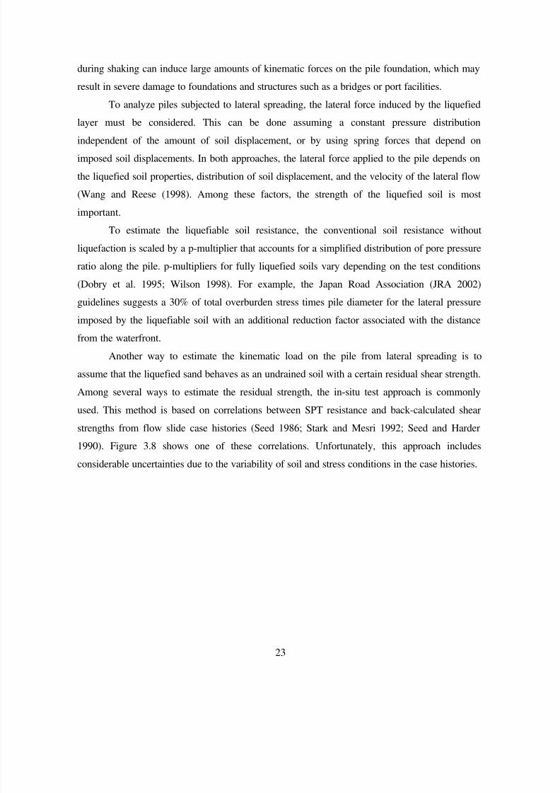
Figure 3.8 Relationship between residual strength and corrected SPT resistance (Seed and
Harder 1990)............................................................................................................ 24
Figure 3.9 Pile foundation failure of Yachiyo bridge due to kinematic loading (after
Hamada 1992).......................................................................................................... 28
Figure 3.10 Schematic of pile alignment in group...................................................................... 30
Figure 3.11 Design chart for p-multipliers (after Mokwa 1999) ................................................ 31
Figure 3.12 Schematic of rotational soil resistance due to pile cap rotation .............................. 32
Figure 3.13 Illustration of axial load transfer in a pile (after Vijayvergiya 1997)...................... 32
Figure 3.14 Illustration of axial load transfer mechanism in a pile (after Vijayvergiya 1997)... 36
Figure 3.15 Typical load-movement characteristics of an axially loaded pile (after
Vijayvergiya 1997).................................................................................................. 37
Figure 3.16 Normalized t-z (or f-z) curve for clay and sand (after Vijayvergiya 1997)............. 39
Figure 3.17 Normalized q-z curve for sand and clay (after Vijayvergiya 1997) ........................ 40
Figure 3.18 Lateral stiffness of column with and without rotational restraint at top.................. 41
Figure 3.19 Schematic of seat-type abutment structural components and bridge deck-
abutment–soil interaction ........................................................................................ 44
Figure 3.20 Simplified abutment load-deflection characteristic using initial stiffness and
ultimate resistance in Caltrans’s guideline (after SDC 2004) ................................. 45
Figure 4.1 Testbed bridge configuration (dimensions in meters) ............................................. 48
Figure 4.2 Layer definition and identification .......................................................................... 49
Figure 4.3 SPT profiles of loose sand layer below both embankments.................................... 50
7/21/2019 PEER807 KRAMERArduino Shin
http://slidepdf.com/reader/full/peer807-kramerarduino-shin 11/198
7/21/2019 PEER807 KRAMERArduino Shin
http://slidepdf.com/reader/full/peer807-kramerarduino-shin 12/198
xiii
Figure 6.14 p-y time histories during earthquake excitation—Erzincan motion........................ 82
Figure 6.15 p-y curves during earthquake excitation—Erzincan motion. .................................. 82
Figure 6.16 Pile cap resistance curves—Erzincan motion.......................................................... 83
Figure 7.1 Example of input motion used in comprehensive bridge study—Erzincan
motion...................................................................................................................... 86
Figure 7.2 PGA hazard curve.................................................................................................... 89
Figure 7.3 Implied hazard curves for different IMs.................................................................. 91
Figure 7.4 Correlation between lateral pile cap displacement and curvature from
simulations for Northridge 1994, 0.2557 g; unit of curvature = 1/m ...................... 93
Figure 7.5 Components of total uncertainty in EDP estimation ............................................... 94
Figure 7.6 EDP-IM relationships for right abutment slope residual vertical settlement .......... 96
Figure 7.7 EDP-IM relationships for Pier 4 maximum drift..................................................... 97
Figure 7.8 Relative efficiencies of different IMs...................................................................... 98
Figure 7.9 Tornado diagrams for four maximum EDPs: Temblor 1966 motion at
Parkfield (amax= 0.47 g) ......................................................................................... 102
Figure 7.10 Inherent soil variability (after Phoon and Kulhawy 1999) .................................... 106
Figure 7.11 Example of generated Gaussian fields................................................................... 107
Figure 7.12 Development of random field for friction angle in loose, saturated sand layer;
(a) mean friction angle, (b) residual friction angle, (c) total friction angle. .......... 109
Figure 7.13 Variation of horizontal subsurface displacements for ground motions with
(a) 15-yrs return period, (b) 72-yrs return period, (c) 475-yrs return period, and
(d) 2475-yrs return period...................................................................................... 114
Figure 7.14 Horizontal displacements at tops and bottoms of Piers 1 and 4. Note that
absolute displacement of Pier 4 (bottom) is larger than that of Pier 1, but
difference between the top and bottom displacements is larger at Pier 1 than
Pier 4...................................................................................................................... 115
Figure 7.15 Relationship between PGV and (a) expansion joint displacement at left
abutment, (b) expansion joint displacement at right abutment.............................. 116
Figure 7.16 Relationship between PGV and pile cap horizontal displacement for (a) Pier 0
(left abutment), (b) Pier 1, (c) Pier 2, and (d) Pier 3, (e) Pier 4, and (f) Pier 5
(right abutment). .................................................................................................... 117
7/21/2019 PEER807 KRAMERArduino Shin
http://slidepdf.com/reader/full/peer807-kramerarduino-shin 13/198
xiv
Figure 7.17 Relationship between CAV5 and (a) vertical gap at left abutment and
(b) vertical gap at right abutment. ......................................................................... 118
Figure 7.18 Relationship between PGV and column drift for (a) Pier 1, (b) Pier 2,
(c) Pier 3, and (d) Pier 4. ....................................................................................... 119
Figure 7.19 Location of maximum pile bending moment in Pile 0 at left abutment ................ 120
Figure 7.20 Location of maximum pile curvatures in Pile 4 and Pile 5 at right abutment ....... 121
Figure 7.21 Variation of median pier drift with PGV............................................................... 122
Figure 8.1 Mean annual rates of exceedance of repair cost ratio, RCR, for different pile
groups: (a) left abutment, (b)–(e) interior columns, and (f) right abutment.
DM hazard curves for each pile group obtained considering most efficient
IM: (a) CAV5, (b) PGV, (c) CAV5, (d) PGA, (e) Ia, (f) CAV5 ............................. 132
Figure 9.1 PGV hazard curve for highway testbed bridge site. .............................................. 144
Figure 9.2 Distribution of DV|IM (16th, 50th, and 84th percentile curves shown) for
highway testbed bridge site for liquefaction case.................................................. 144
Figure 9.3 Total repair cost ratio hazard curve for liquefaction case obtained from
convolution of relationships shown in Figures 9.1 and 9.2................................... 145
Figure 9.4 Deaggregated conditional repair costs for testbed highway bridge in
liquefaction case. ................................................................................................... 146
Figure 9.5 Deaggregated conditional repair costs for testbed highway bridge for 475-yrs
return period in liquefaction case. ......................................................................... 146
Figure 9.6 Distribution of DV|IM for highway testbed bridge site for non-liquefaction
case. ....................................................................................................................... 148
Figure 9.7 Total repair cost ratio hazard curve for non-liquefaction case. ............................. 148
Figure 9.8 Deaggregated conditional repair costs for testbed highway bridge in non-
liquefaction case. ................................................................................................... 149
Figure 9.9 Deaggregated conditional repair costs for testbed highway bridge for 475-yrs
return period in non-liquefaction case. .................................................................. 149
Figure 9.10 Distribution of DV|IM for highway testbed bridge site for fixed-base case ......... 150
Figure 9.11 Total repair cost ratio hazard curve for fixed-base case........................................ 151
Figure 9.12 Deaggregated conditional repair costs for testbed highway bridge in fixed-base
case. ....................................................................................................................... 151
7/21/2019 PEER807 KRAMERArduino Shin
http://slidepdf.com/reader/full/peer807-kramerarduino-shin 14/198
xv
Figure 9.13 Deaggregated conditional repair costs for testbed highway bridge for 475-yrs
return period. ......................................................................................................... 152
Figure 9.14 Effect of different soil conditions on total repair cost ratio hazard curves............ 153
Figure 9.15 DV|IM relationship for liquefaction case with different fractions of actual
uncertainty. ............................................................................................................ 154
Figure 9.16 DV|IM relationship for non-liquefaction case with different fractions of actual
uncertainty. ............................................................................................................ 154
Figure 9.17 Effects of different levels of uncertainty in DV|IM on loss hazard for
liquefaction case. ................................................................................................... 154
Figure 9.18 Effects of different levels of uncertainty in DV|IM on loss hazard for
liquefaction case. ................................................................................................... 154
Figure A.1 Schematic illustration of PEER PBEE components. ............................................. A-1
Figure A.2 Variation of right abutment vertical displacement with (l-r) peak ground
velocity, Arias intensity, and CAV5. ..................................................................... A-5
Figure A.3 Variation of Pier 4 maximum drift with (l-r) peak ground velocity, Arias
intensity, and CAV5...............................................................................................A-5
Figure A.4 Fragility surface for testbed bridge. White lines indicate fragility curves for
repair cost ratios of 20%, 40%, 60%, 80%, and 90%............................................ A-7
Figure A.5 Loss curve for testbed bridge.................................................................................A-8
7/21/2019 PEER807 KRAMERArduino Shin
http://slidepdf.com/reader/full/peer807-kramerarduino-shin 15/198
xvii
LIST OF TABLES
Table 3.1 Representative values of 50ε for normally consolidated clays—Peck et al.
(1974) (after Reese and Van Impe 2001). ............................................................... 17
Table 3.2 Representative values of 50ε for overconsolidated clays (after Reese and
Van Impe 2001). ...................................................................................................... 17
Table 3.3 Representative values of pyk for sand (after Reese and Van Impe 2001)............... 18
Table 3.4 Recommended p-multipliers for pseudo-static analysis (after
Brandenberg 2005). ................................................................................................. 26
Table 3.5 Typical values of soil adhesion factor, a (after NAVFAC 1982)............................ 35
Table 3.6 Recommended parameters for cohesionless siliceous soil (after API 1993)........... 39
Table 4.1 Soil types and properties.......................................................................................... 49
Table 4.2 SPT profiles below embankments ........................................................................... 50
Table 5.1 Summary of PIMY material parameter values used for cohesive soil .................... 56
Table 5.2 Summary of PDMY material parameter values used for granular soils.................. 57
Table 7.1 Magnitude-corrected PGA....................................................................................... 87
Table 7.2 I-880 input motion characteristics (four hazards).................................................... 88
Table 7.3 Intensity measures ................................................................................................... 90
Table 7.4 IM hazard curve coefficients for I-880 input motions............................................. 91
Table 7.5 EDP list.................................................................................................................... 92
Table 7.6 Summary of EDP median coefficients and record-to-record uncertainty for
power-law median response model, EDP = a IMb.................................................. 99
Table 7.7 Input parameter uncertainties ................................................................................ 100
Table 7.8 Correlation coefficients for uncertain input parameters. ....................................... 104
Table 7.9 Summary of parametric uncertainty ...................................................................... 105
Table 7.10 Summary of spatial variability uncertainty (loose sand plus clay)........................ 110
Table 7.11 Summary of spatial variability uncertainty (loose sand) ....................................... 111
Table 7.12 Summary of spatial variability uncertainty (clay) ................................................. 112
Table 7.13 Summary of EDP hazard curve: exponential coefficient ...................................... 123
Table 8.1 Damage probability matrix.................................................................................... 126
Table 8.2 Loss probability matrix.......................................................................................... 127
7/21/2019 PEER807 KRAMERArduino Shin
http://slidepdf.com/reader/full/peer807-kramerarduino-shin 16/198
xviii
Table 8.3 EDP ranges corresponding to different damage states; where EDP=foundation
lateral displacement ............................................................................................... 128
Table 8.4 Damage probabilities. ............................................................................................ 129
Table 8.5 Loss probabilities................................................................................................... 129
Table 8.6 Tabular listing of mean annual rates of exceedance and return period for
various damage states. ........................................................................................... 130
Table 8.7 Estimated loss levels.............................................................................................. 131
Table 9.1 Performance groups and associated EDPs............................................................. 136
Table 9.2 Column damage states based on maximum tangential drift ratio.......................... 137
Table 9.3 Column damage states based on residual tangential drift ratio. ............................ 137
Table 9.4 Expansion joint damage states............................................................................... 138
Table 9.5 Bearing damage states. .......................................................................................... 138
Table 9.6 Abutment backwall damage states. ....................................................................... 139
Table 9.7 Approach slab damage states................................................................................. 139
Table 9.8 Bridge deck damage states. ................................................................................... 140
Table 9.9 Pile foundation damage states. .............................................................................. 140
Table 9.10 Column repair methods and costs.......................................................................... 141
Table 9.11 Expansion joint repair methods and costs. ............................................................ 142
Table 9.12 Bearing repair methods and costs.......................................................................... 142
Table 9.13 Abutment backwall repair methods and costs. ...................................................... 142
Table 9.14 Approach slab repair methods and costs. .............................................................. 142
Table 9.15 Bridge deck repair methods and costs. .................................................................. 142
Table 9.16 Pile foundation repair methods and costs. ............................................................. 143
7/21/2019 PEER807 KRAMERArduino Shin
http://slidepdf.com/reader/full/peer807-kramerarduino-shin 17/198
7/21/2019 PEER807 KRAMERArduino Shin
http://slidepdf.com/reader/full/peer807-kramerarduino-shin 18/198
2
1.2 PERFORMANCE-BASED EARTHQUAKE ENGINEERING
Most bridges are “owned” (i.e., designed, financed, constructed, operated, and maintained) by
public agencies that are responsible for multiple bridges and the network of roadways that
connect them. Such agencies need to evaluate the potential seismic performance of their entire
transportation systems in order to determine which elements of the system are most vulnerable to
earthquake damage. To an owner, measures of performance in economic terms are most useful
in providing guidance with respect to decisions on investment in repair or replacement of
bridges.
The concept of performance-based earthquake engineering (PBEE) provides a framework
for direct, quantitative estimation of losses due to earthquake shaking. PBEE allows an
integrated assessment of earthquake ground shaking hazards, bridge system response, physicalbridge damage, and resulting economic loss. By explicitly considering the various uncertainties
in ground motion, response, damage, and loss estimation, a PBEE analysis can provide an
unbiased, objective, and quantifiable estimate of earthquake risk. The results of such analyses
can be used to evaluate economic exposure, and to evaluate the relative costs and benefits of
various mitigation/retrofit measures (including the option of no mitigation or retrofit).
The Pacific Earthquake Engineering Research (PEER) Center has developed a PBEE
framework that allows estimation of response, damage, and loss to be made in a modular
manner. This framework has numerous advantages including the ability to allow the loss
estimation process to be divided into discipline-specific components with relatively clear
indications of required interdisciplinary interactions, as well as the ability to track the main
factors that contribute to estimated losses. The framework is probabilistic in nature, i.e., it
requires identification and characterization of all uncertainties involved in response, damage, and
loss estimation, and propagates those uncertainties in a manner that reflects their effects on
estimated losses. The expected losses in a given exposure period can be shown to increase with
increasing levels of uncertainty; as a result, reduction of uncertainty in different components of
the PBEE evaluation can lead to reductions in expected losses.
Response and damage estimation are among the most prominent activities of earthquake
engineers in the PBEE process. Geotechnical and structural engineers are usually involved in the
estimation of bridge response and damage due to different levels of earthquake ground motion.
Various approaches to response prediction are used, for example, in geotechnical engineering
7/21/2019 PEER807 KRAMERArduino Shin
http://slidepdf.com/reader/full/peer807-kramerarduino-shin 19/198
3
practice. These range from very simple prescriptive models to somewhat more complicated
empirical models to simplified analytical models to complicated analytical models. In concept,
the uncertainties in predicted response for these different models should decrease with increasing
level of model rigor. The current state of geotechnical engineering practice, however, has not
advanced to the point where these uncertainty levels can be accurately quantified. As a result,
the relative benefits and drawbacks of performing more rigorous response analyses have not
been demonstrated.
1.3 OBJECTIVES OF THE STUDY
The objective of the investigation described in this report was to apply the PEER PBEE
methodology to the evaluation of a bridge founded on liquefiable soils subject to lateralspreading. This investigation used high-level finite element-based soil-foundation-structure
interaction analyses to predict bridge system response, and then used that response to predict
physical damage and economic loss. A parallel investigation, conducted at UC Berkeley
(Ledezma and Bray 2007), used simplified response analyses to estimate physical damage and
then economic loss.
The investigation was intended to document the procedures used to apply the PEER
methodology when a rigorous response analyses is performed, and to identify the costs and
benefits of performing such analyses.
1.4 ORGANIZATION
The report is organized in a manner that should allow a practicing engineer to understand the
PEER PBEE framework and its application to the problem of estimating bridge performance.
Following the introduction, Chapter 2 provides a review of PBEE and introduces the
PEER PBEE framework with descriptions of response, damage, and loss estimation. Chapter 3
describes basic concepts of soil-pile-structure interaction analysis. The notion of p-y curves and
their characteristics for both non-liquefiable and liquefiable soils is described, as is their use in
analysis of laterally loaded piles and pile groups. Similar rheological elements for vertically
loaded piles and for abutments are also introduced. The characteristics of a testbed bridge in a
hypothetical (but realistic) soil profile are described in Chapter 4. Chapter 5 describes the
7/21/2019 PEER807 KRAMERArduino Shin
http://slidepdf.com/reader/full/peer807-kramerarduino-shin 20/198
4
development of a detailed finite element model of the soil profile, foundations, abutments, and
bridge superstructure. Chapter 6 describes a series of validation analyses of the finite element
model, and then goes on to describe the results of an extensive series of response analyses for
different input ground motions. In Chapter 7 variations of median response level for numerous
response metrics are presented, and the dispersion of computed responses about those median
values are characterized. The effects of uncertainties in model parameters and of spatial
variability are also described. The performance of the bridge foundations are expressed in terms
of damage states and loss levels in a discrete framework described in Chapter 8. Chapter 9
describes damage and loss for the entire bridge in a continuous framework. The loss levels for
cases in which liquefaction is allowed to occur and not allowed to occur, and for the case in
which the bridge is essentially assumed to be founded on rock, are all described and compared.
The effects of uncertainty in the response model on predicted losses are also discussed. Finally,
Chapter 10 summarizes the investigation and the conclusions that can be drawn from it.
7/21/2019 PEER807 KRAMERArduino Shin
http://slidepdf.com/reader/full/peer807-kramerarduino-shin 21/198
5
2 Performance-Based Earthquake Engineering
2.1 INTRODUCTION
Performance-based earthquake engineering (PBEE) refers to an emerging paradigm in which the
“performance” of a system of interest can be quantified and predicted on a discrete or continuous
basis. The notion of performance means different things to different stakeholders, and an
important goal of PBEE is to allow performance to be expressed using terms and quantities that
are of interest and meaning to a wide range of earthquake professionals and decision-makers.
Implicit in the development of PBEE is the idea that performance can be quantified and
predicted with sufficient accuracy to allow decisions regarding design, repair, retrofit, and
replacement to be made with confidence. Continuing developments in the field of earthquake
engineering are providing engineers with the tools necessary to make such predictions. The full
development of PBEE will allow performance to be expressed in terms of “risk” i.e., in terms
that reflect both the direct and indirect losses associated with the occurrence of earthquakes.
Such losses can be expressed in terms of casualties, economic losses, and lost time.
2.2 PEER FRAMEWORK
PBEE is generally formulated in a probabilistic framework to account for the many uncertainties
involved in estimating the risk associated with earthquake hazards at a particular site. The term
“risk” is used in this report to denote loss, which can be expressed in terms of cost, fatalities, or
other measures. The term “hazard” is used to describe levels of ground shaking, system
response, and/or physical damage, but has no specific connotation of loss. Minimizing the
uncertainty in hazard and risk estimates requires minimizing the uncertainties in the variables
and the relationships between the variables that go into their calculation.
The PBEE framework developed by the Pacific Earthquake Engineering Research Center
(PEER) computes risk as a function of ground shaking through the use of several intermediate
7/21/2019 PEER807 KRAMERArduino Shin
http://slidepdf.com/reader/full/peer807-kramerarduino-shin 22/198
6
variables. The ground motion is characterized by an intensity measure, IM , which could be any
one of a number of ground motion parameters (e.g., PGA, Arias intensity, S a, etc.). The effects
of the IM on a system of interest are expressed in terms that make sense to engineers in the form
of engineering demand parameters, or EDPs (e.g., interstory drift, settlement, etc.). The physical
effects associated with the EDPs are expressed in terms of damage measures, or DM s (e.g., crack
width, spalling). Finally, the risk associated with the DM is expressed in a form that is useful to
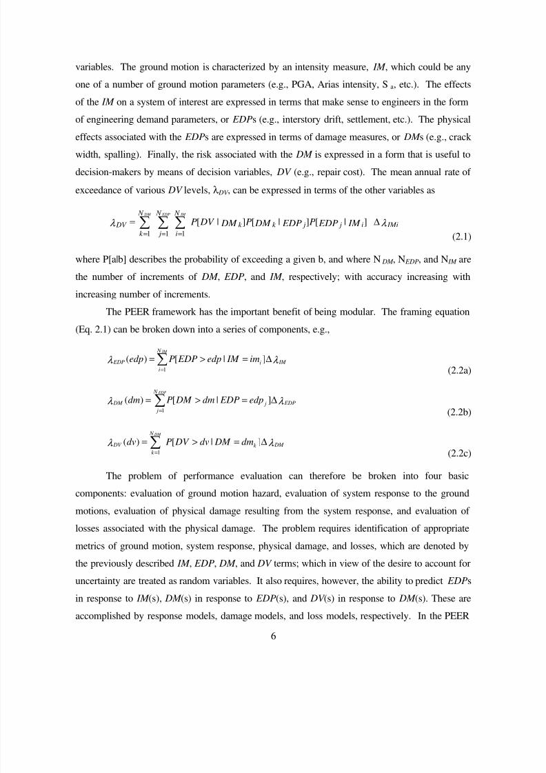
decision-makers by means of decision variables, DV (e.g., repair cost). The mean annual rate of
exceedance of various DV levels, λ DV , can be expressed in terms of the other variables as
λ λ IMii j jk k
N
i
N
j
N
k
DV IM EDPP EDP DM P DM DV P IM EDP DM
∆= ∑∑∑===
]|[]|[]|[111 (2.1)
where P[a|b] describes the probability of exceeding a given b, and where N DM , N EDP, and N IM are
the number of increments of DM , EDP, and IM , respectively; with accuracy increasing with
increasing number of increments.
The PEER framework has the important benefit of being modular. The framing equation
(Eq. 2.1) can be broken down into a series of components, e.g.,
λ λ IM i
N
i
EDP im IM edp EDPPedp IM
∆=>=∑=
]|[)(1 (2.2a)
λ λ EDP j
N
j
DM edp EDPdm DM Pdm EDP
∆=>= ∑=
]|[)(1 (2.2b)
λ λ DM k
N
k
DV dm DM dv DV Pdv DM
∆=>=∑=
]|[)(1 (2.2c)
The problem of performance evaluation can therefore be broken into four basic
components: evaluation of ground motion hazard, evaluation of system response to the ground
motions, evaluation of physical damage resulting from the system response, and evaluation of
losses associated with the physical damage. The problem requires identification of appropriate
metrics of ground motion, system response, physical damage, and losses, which are denoted by
the previously described IM , EDP, DM , and DV terms; which in view of the desire to account for
uncertainty are treated as random variables. It also requires, however, the ability to predict EDPs
in response to IM (s), DM (s) in response to EDP(s), and DV (s) in response to DM (s). These are
accomplished by response models, damage models, and loss models, respectively. In the PEER
7/21/2019 PEER807 KRAMERArduino Shin
http://slidepdf.com/reader/full/peer807-kramerarduino-shin 23/198
7
framework, these models are all formulated probabilistically—for example, the response model
must be able to predict the probability distribution of an EDP for a given IM value.
2.3 RESPONSE PREDICTION
Currently, the structural and geotechnical engineers’ primary contributions to the PBEE process
come primarily in the evaluation of P[ EDP| IM ] as indicated in Equation (2.2a). This process
involves establishing an appropriate IM , which should be one that the EDP(s) of interest are
closely related to (furthermore, the EDP(s) of interest should be the ones that the DM (s) of
interest are closely related to, and the DM (s) of interest should be the ones that the DV (s) of
interest are closely related to). Luco and Cornell (2001) defined efficient intensity measures as
those that produced little dispersion in EDP for a given IM . In other words, an efficient IM is onefor which the uncertainty in EDP| IM is low. The efficiency of IM (s) varies from one type of
problem to another, and can also vary from one EDP to another. Selection of efficient IM (s) is
critical to the reliable and economical implementation of PBEE procedures. Luco and Cornell
(2001) also described sufficient IM (s) as those for which the use of additional ground motion
information does not reduce the uncertainty in EDP| IM . A perfectly sufficient IM would be one
that tells an engineer all he/she needs to know about the motion’s potential for producing a
certain response in a system of interest.
The notions of efficiency and sufficiency are important for the performance-based
evaluation of structures affected by liquefaction hazards because conventional procedures for
evaluating liquefaction potential are based on an IM (PGA) that is moderately efficient but
distinctly insufficient. The moderate efficiency comes from the fact that liquefaction potential is
evaluated using peak ground acceleration, which is a measure of the high-frequency content of a
ground motion. The generation of excess porewater pressure, however, is clearly related to shear
strain amplitude, which basic wave propagation concepts (in a linear system) indicate is
proportional to particle velocity. Because of the smoothing effects of integration (from
acceleration to velocity), strain amplitude is more closely related to intermediate frequencies
(often in the range of 1–2 Hz). The insufficiency comes from the fact that excess pore pressures
increase incrementally during an earthquake; hence the duration of a ground motion, which is not
reflected in peak acceleration alone, affects excess porewater pressure generation. In the earliest
modern procedures for liquefaction potential evaluation, the effects of duration were accounted
7/21/2019 PEER807 KRAMERArduino Shin
http://slidepdf.com/reader/full/peer807-kramerarduino-shin 24/198
8
for by the introduction of a magnitude scaling factor. The need for the magnitude scaling factor
is, in and of itself, evidence that peak acceleration is insufficient for the prediction of
liquefaction potential.
Structural response is generally less sensitive to duration than liquefaction, so IM s that
reflect anticipated peak response can be relatively efficient. First-mode spectral acceleration,
Sa(To), is frequently used as a scalar IM for structural response evaluation. For structures of
intermediate fundamental period, peak velocity often correlates strongly to Sa(To) and can
therefore serve as an efficient IM that is computed directly from the ground motion (rather than
through the filter of SDOF system response on which Sa(To) is based).
2.4 DAMAGE PREDICTION
Prediction of the physical damage associated with various levels of system response is a
relatively new and difficult task. Physical damage is generally associated with nonlinear,
inelastic response; ground shaking that produces only linear, elastic response is unlikely to cause
physical damage to a structure or its foundations, although it is possible that some damage to
contents could occur.
Damage is estimated through the use of damage models, which can be continuous or
discrete. A continuous damage model would define damage in terms of some continuous
variable, e.g., crack width in a concrete column or beam. By defining some capacity in terms of
a limiting level of response that produces a given amount of damage and characterizing the
uncertainty in damage, Equation (2.2b) can be used to convolve a continuous damage function
with an EDP hazard curve to obtain a damage hazard curve.
For many forms of damage, however, specific capacity distributions are not available. In
such cases, damage can be divided into several discrete categories, or damage states. Discrete
damage states can be defined by quantitative ranges of some DM , for example, crack widths of
0–1 mm, 1–2 mm, 2–4 mm, etc. Alternatively, damage states can be defined qualitatively, e.g.,
low, medium, or high. The expression of damage states is often performed heuristically based on
experience, intuition, and engineering judgment. In the absence of detailed, quantitative damage
data, it may be necessary to use expert opinion to identify damage states. Upsall (2006) polled
two groups of geotechnical engineers—a group of random practitioners in the Seattle,
Washington, area and a group of experienced post-earthquake reconnaissance leaders—and
7/21/2019 PEER807 KRAMERArduino Shin
http://slidepdf.com/reader/full/peer807-kramerarduino-shin 25/198
9
found significant differences in their estimates of the levels of permanent deformations required
to produce different qualitative damage states.
2.5 LOSS PREDICTION
The estimation of earthquake-induced losses, whether expressed in terms of casualties, direct
and/or indirect losses, or downtime) is also in a relatively undeveloped state. Loss estimation is
typically best performed by persons other than those who are best suited to evaluating response
and physical damage. Construction estimators, insurance adjustors, real estate appraisers, and
others who deal with damaged structures are more likely to be capable of accurate loss
estimation than typical design engineers. The advancement of PBEE will clearly require
increased interaction between engineers and loss estimators.The estimation of even direct economic losses, which are arguably the easiest types of
losses to estimate, is far from simple. In addition to the effects of such uncertain variables as
future material, labor, and capital costs, loss functions are also discontinuous. For example,
repair costs associated with epoxying of cracks in a bridge girder would suddenly drop to zero if
damage is sufficiently high that the girder would be replaced. Many repair/replacement costs are
highly correlated, but studies that would better define the relationships between various
damage/loss variables for both simple and complex structures have not yet been performed.
In the absence of detailed loss estimation procedures, it is often necessary to use expert
opinion to develop working loss models. The quality of the resulting loss estimates should
consider the efficiencies and sufficiencies of the variables used to estimate losses.
2.6 SUMMARY
The PEER framework for performance-based earthquake engineering provides a useful, rational,
and modular approach to performance prediction. Implementation of the framework involves the
identification of suitable parameters for describing ground motion system response, physical
damage, and losses. It also requires the prediction of response given ground motion, physical
damage given response, and loss given physical damage. The framework further requires that
uncertainty in these parameters, and the relationships between them, be characterized and
properly accounted for in the analyses.
7/21/2019 PEER807 KRAMERArduino Shin
http://slidepdf.com/reader/full/peer807-kramerarduino-shin 26/198
11
3 Seismic Soil-Pile-Structure Interaction
3.1 INTRODUCTION
Typical bridges consist of the bridge structure, pile/drilled shafts or spread footing foundations,
abutment structures, and the supporting soil. During earthquakes, the individual components
interact with each other and affect the global response of the bridge. In this chapter, relevant
aspects related to lateral soil-pile interaction and soil-abutment-bridge interaction are briefly
reviewed and discussed. Since p-y curves are important in modeling soil-pile-structure
interaction, this topic is covered in more detail. Other topics reviewed in this chapter include the
lateral response of piles and pile groups, soil-pile-structure interaction associated with structural
stiffness, and soil-abutment-bridge interaction.
3.2 SOIL-PILE INTERACTION MODELING
Soils and pile foundations interact with each other under both static and dynamic loading
conditions. The interaction is complex, and complete evaluation requires resources that are rarely
available to practicing engineers. As a result, simplified models, which attempt to capture the
main aspects of soil-pile interaction, have been developed. These models have been shown to
work well for static and relatively slow cyclic loads (such as wave loads, typically encountered
in pile-supported offshore structures), and can also be applied, with consideration of inertial
effects, to problems including seismic soil-pile interaction. Among these models, those based on
the static/dynamic beam-on-nonlinear-Winkler-foundation (BNWF) method, often referred to as
the p-y method, are commonly used to model soil-pile interaction problems and deserve special
attention.
7/21/2019 PEER807 KRAMERArduino Shin
http://slidepdf.com/reader/full/peer807-kramerarduino-shin 27/198
12
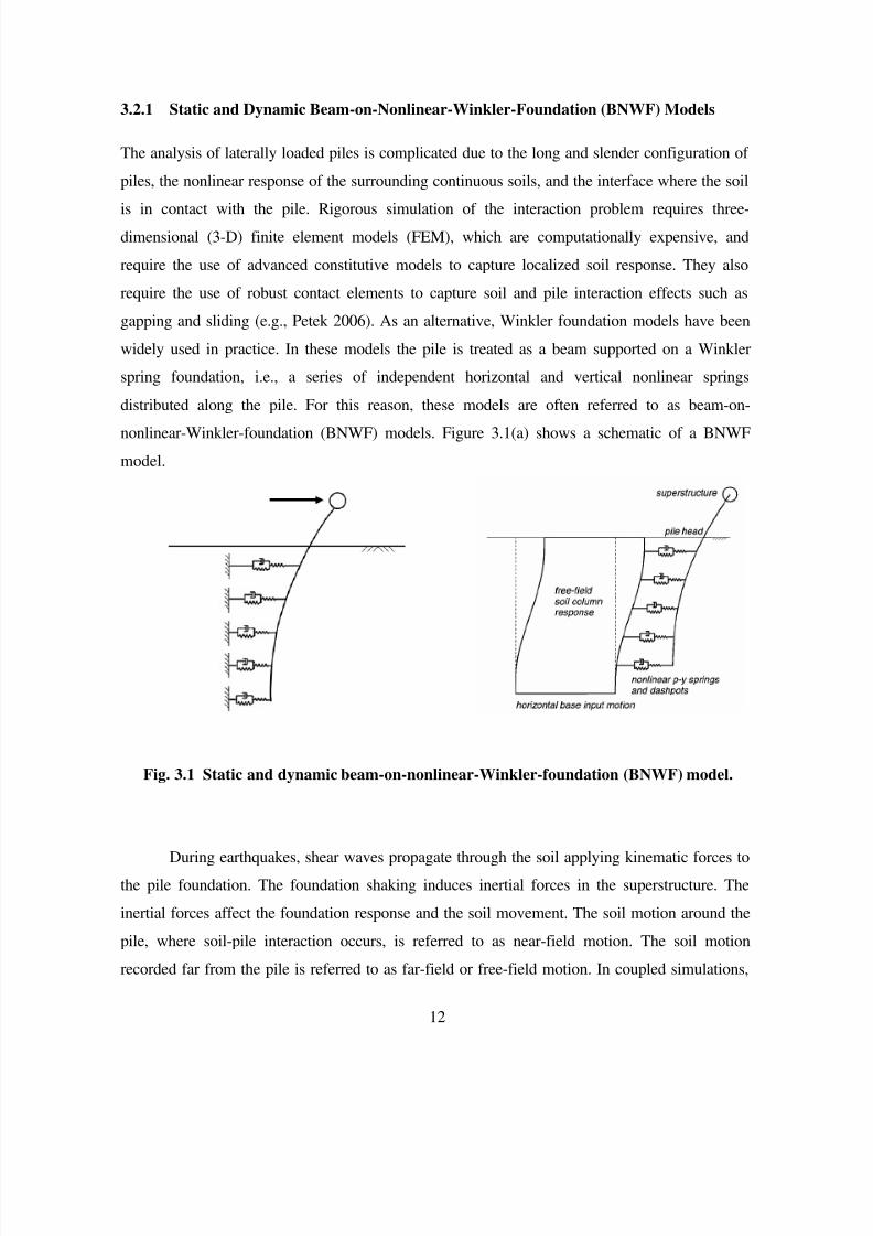
3.2.1 Static and Dynamic Beam-on-Nonlinear-Winkler-Foundation (BNWF) Models
The analysis of laterally loaded piles is complicated due to the long and slender configuration of
piles, the nonlinear response of the surrounding continuous soils, and the interface where the soil
is in contact with the pile. Rigorous simulation of the interaction problem requires three-
dimensional (3-D) finite element models (FEM), which are computationally expensive, and
require the use of advanced constitutive models to capture localized soil response. They also
require the use of robust contact elements to capture soil and pile interaction effects such as
gapping and sliding (e.g., Petek 2006). As an alternative, Winkler foundation models have been
widely used in practice. In these models the pile is treated as a beam supported on a Winkler
spring foundation, i.e., a series of independent horizontal and vertical nonlinear springs
distributed along the pile. For this reason, these models are often referred to as beam-on-nonlinear-Winkler-foundation (BNWF) models. Figure 3.1(a) shows a schematic of a BNWF
model.
Fig. 3.1 Static and dynamic beam-on-nonlinear-Winkler-foundation (BNWF) model.
During earthquakes, shear waves propagate through the soil applying kinematic forces to
the pile foundation. The foundation shaking induces inertial forces in the superstructure. The
inertial forces affect the foundation response and the soil movement. The soil motion around the
pile, where soil-pile interaction occurs, is referred to as near-field motion. The soil motion
recorded far from the pile is referred to as far-field or free-field motion. In coupled simulations,
7/21/2019 PEER807 KRAMERArduino Shin
http://slidepdf.com/reader/full/peer807-kramerarduino-shin 28/198
13
where the pile and soil are connected by interface springs, it is assumed that a soil column
provides the free-field motion and that the soil-pile-structure interaction occurs at the interface
springs. Alternatively, free-field motions can be calculated separately along the pile depth and
the corresponding displacement time histories can be applied to p-y springs. This idea is
illustrated in the dynamic Beam-on-nonlinear-Winkler-foundation (BNWF) model shown in
Figure 3.1(b).
3.3 p-y CURVES
To completely define the BNWF model it is important to establish accurate p-y curves. In this
section two cases are considered: (1) a pile subjected to monotonic and cyclic loads at the pile
head and (2) a pile embedded in liquefiable soil and subjected to earthquake excitations andlateral spreading. To analyze the first case, conventional p-y curves are introduced. For the
earthquake problem, since there are not yet well-established p-y curves for liquefiable soil,
several experimental observations are discussed.
3.3.1 Conventional p-y Curves for Piles Subjected to Static and Cyclic Loading
To capture the lateral response of piles, soil reaction force versus pile displacement (i.e., p-y)
relationships are commonly used together with beam elements in static and dynamic BNWF
models. In general these curves are based on field tests, laboratory model tests, and analytical
solutions. The pile displacement (y) and soil-resisting force per unit length (p) can be back-
calculated from measured or calculated bending moments by double-differentiating and double-
integrating the governing equilibrium differential equation. That is,
)(2
2
z M dz
d p =
(3.1)
and, assuming linear bending behavior,
EI
z M y
dz
d )(2
2
= (3.2)
7/21/2019 PEER807 KRAMERArduino Shin
http://slidepdf.com/reader/full/peer807-kramerarduino-shin 29/198
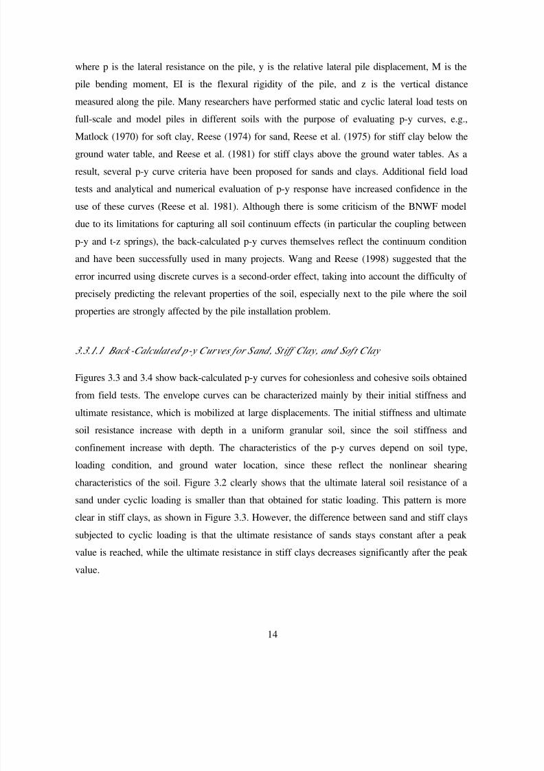
14
where p is the lateral resistance on the pile, y is the relative lateral pile displacement, M is the
pile bending moment, EI is the flexural rigidity of the pile, and z is the vertical distance
measured along the pile. Many researchers have performed static and cyclic lateral load tests on
full-scale and model piles in different soils with the purpose of evaluating p-y curves, e.g.,
Matlock (1970) for soft clay, Reese (1974) for sand, Reese et al. (1975) for stiff clay below the
ground water table, and Reese et al. (1981) for stiff clays above the ground water tables. As a
result, several p-y curve criteria have been proposed for sands and clays. Additional field load
tests and analytical and numerical evaluation of p-y response have increased confidence in the
use of these curves (Reese et al. 1981). Although there is some criticism of the BNWF model
due to its limitations for capturing all soil continuum effects (in particular the coupling between
p-y and t-z springs), the back-calculated p-y curves themselves reflect the continuum condition
and have been successfully used in many projects. Wang and Reese (1998) suggested that the
error incurred using discrete curves is a second-order effect, taking into account the difficulty of
precisely predicting the relevant properties of the soil, especially next to the pile where the soil
properties are strongly affected by the pile installation problem.
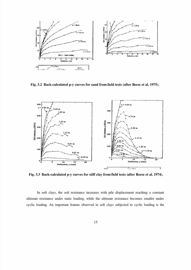
3.3.1.1 Back -Calculated p-y Curves for Sand, Stiff Clay, and Soft Clay
Figures 3.3 and 3.4 show back-calculated p-y curves for cohesionless and cohesive soils obtained
from field tests. The envelope curves can be characterized mainly by their initial stiffness and
ultimate resistance, which is mobilized at large displacements. The initial stiffness and ultimate
soil resistance increase with depth in a uniform granular soil, since the soil stiffness and
confinement increase with depth. The characteristics of the p-y curves depend on soil type,
loading condition, and ground water location, since these reflect the nonlinear shearing
characteristics of the soil. Figure 3.2 clearly shows that the ultimate lateral soil resistance of a
sand under cyclic loading is smaller than that obtained for static loading. This pattern is more
clear in stiff clays, as shown in Figure 3.3. However, the difference between sand and stiff clays
subjected to cyclic loading is that the ultimate resistance of sands stays constant after a peak
value is reached, while the ultimate resistance in stiff clays decreases significantly after the peak
value.
7/21/2019 PEER807 KRAMERArduino Shin
http://slidepdf.com/reader/full/peer807-kramerarduino-shin 30/198
15
Fig. 3.2 Back-calculated p-y curves for sand from field tests (after Reese et al. 1975).
Fig. 3.3 Back-calculated p-y curves for stiff clay from field tests (after Reese et al. 1974).
In soft clays, the soil resistance increases with pile displacement reaching a constant
ultimate resistance under static loading, while the ultimate resistance becomes smaller under
cyclic loading. An important feature observed in soft clays subjected to cyclic loading is the
7/21/2019 PEER807 KRAMERArduino Shin
http://slidepdf.com/reader/full/peer807-kramerarduino-shin 31/198
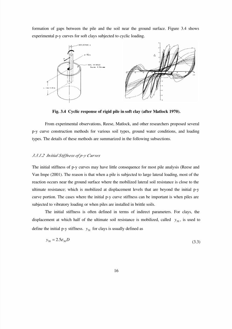
16
formation of gaps between the pile and the soil near the ground surface. Figure 3.4 shows
experimental p-y curves for soft clays subjected to cyclic loading.
Fig. 3.4 Cyclic response of rigid pile in soft clay (after Matlock 1970).
From experimental observations, Reese, Matlock, and other researchers proposed several
p-y curve construction methods for various soil types, ground water conditions, and loading
types. The details of these methods are summarized in the following subsections.
3.3.1.2 In itial Stif fness of p-y Curves
The initial stiffness of p-y curves may have little consequence for most pile analysis (Reese and
Van Impe (2001). The reason is that when a pile is subjected to large lateral loading, most of the
reaction occurs near the ground surface where the mobilized lateral soil resistance is close to the
ultimate resistance; which is mobilized at displacement levels that are beyond the initial p-y
curve portion. The cases where the initial p-y curve stiffness can be important is when piles are
subjected to vibratory loading or when piles are installed in brittle soils.
The initial stiffness is often defined in terms of indirect parameters. For clays, the
displacement at which half of the ultimate soil resistance is mobilized, called 50 y , is used to
define the initial p-y stiffness. 50 y for clays is usually defined as
D y 5050 5.2 ε = (3.3)

7/21/2019 PEER807 KRAMERArduino Shin
http://slidepdf.com/reader/full/peer807-kramerarduino-shin 32/198
17
where ε50 represents the strain corresponding to one half of the undrained strength and D is pile
diameter. Table 3.1 and 3.2 present typical 50ε values for normally- and overconsolidated clays,
respectively.
For sands, Reese et al. (1974) suggest an initial p-y stiffness equal to pyk times depth.
Table 3.3 presents typical pyk values for sands.
Table 3.1 Representative values of 50ε for normally consolidated clays—Peck et al. (1974)
(after Reese and Van Impe 2001).
clay
average undrained
shear strength, (kPa)
50ε
soft clay < 48 0.020
medium clay 48–96 0.010
stiff clay 96–192 0.005
Table 3.2 Representative values of 50ε for overconsolidated clays (after Reese and Van
Impe 2001).
average undrained
shear strength, (kPa)
50ε
overconsolidated 50–100 0.007
clay 100–200 0.005
300–400 0.004
7/21/2019 PEER807 KRAMERArduino Shin
http://slidepdf.com/reader/full/peer807-kramerarduino-shin 33/198
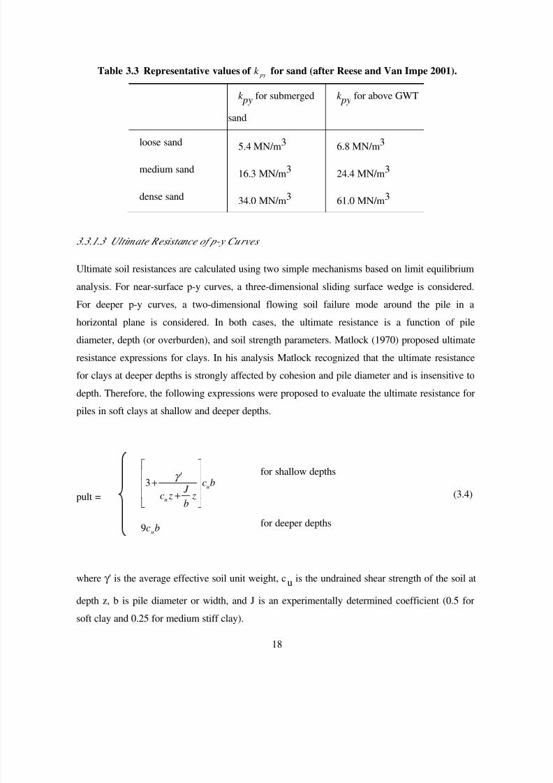
18
Table 3.3 Representative values of pyk for sand (after Reese and Van Impe 2001).
k py for submerged
sand
k py for above GWT
loose sand 5.4 MN/m3 6.8 MN/m3
medium sand 16.3 MN/m3 24.4 MN/m3
dense sand 34.0 MN/m3 61.0 MN/m3
3.3.1.3
Ultimate Resistance of p-y Curves
Ultimate soil resistances are calculated using two simple mechanisms based on limit equilibrium
analysis. For near-surface p-y curves, a three-dimensional sliding surface wedge is considered.
For deeper p-y curves, a two-dimensional flowing soil failure mode around the pile in a
horizontal plane is considered. In both cases, the ultimate resistance is a function of pile
diameter, depth (or overburden), and soil strength parameters. Matlock (1970) proposed ultimate
resistance expressions for clays. In his analysis Matlock recognized that the ultimate resistance
for clays at deeper depths is strongly affected by cohesion and pile diameter and is insensitive to
depth. Therefore, the following expressions were proposed to evaluate the ultimate resistance for
piles in soft clays at shallow and deeper depths.
for shallow depths
pult =
bc
zb
J zc
u
u
++
'3
γ
bcu9 for deeper depths
(3.4)
where γ ′ is the average effective soil unit weight, cu is the undrained shear strength of the soil at
depth z, b is pile diameter or width, and J is an experimentally determined coefficient (0.5 for
soft clay and 0.25 for medium stiff clay).
7/21/2019 PEER807 KRAMERArduino Shin
http://slidepdf.com/reader/full/peer807-kramerarduino-shin 34/198
19
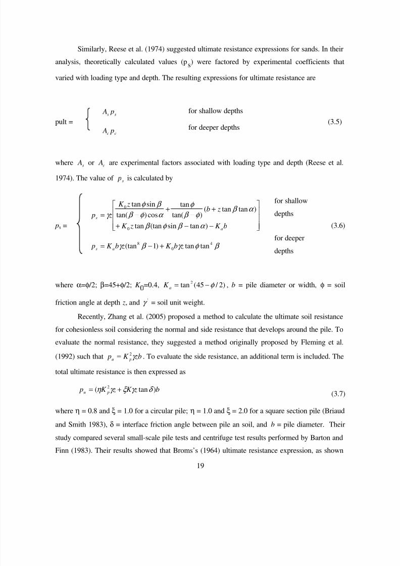
Similarly, Reese et al. (1974) suggested ultimate resistance expressions for sands. In their
analysis, theoretically calculated values (ps) were factored by experimental coefficients that
varied with loading type and depth. The resulting expressions for ultimate resistance are
for shallow depths
pult =ss p A
cc p A for deeper depths(3.5)
where s A or c A are experimental factors associated with loading type and depth (Reese et al.
1974). The value of s p is calculated by
for shallow
depths
ps =
−−+
+−
+−=
bK zK
zb zK
z p
a
s
)tansin(tantan
)tantan()tan(
tan
cos)tan(
sintan
0
0
α β φ β
α β φ β
φ
α φ β
β φ
γ
β φ γ β γ 4
0
8 tantan)1(tan zbK zbK p as +−= for deeper
depths
(3.6)
where α=φ /2; β=45+φ /2; K 0=0.4, )2 / 45(tan 2 φ −=aK , b = pile diameter or width, φ = soil
friction angle at depth z, and 'γ = soil unit weight.
Recently, Zhang et al. (2005) proposed a method to calculate the ultimate soil resistance
for cohesionless soil considering the normal and side resistance that develops around the pile. To
evaluate the normal resistance, they suggested a method originally proposed by Fleming et al.
(1992) such that zbK p pu γ 2= . To evaluate the side resistance, an additional term is included. The
total ultimate resistance is then expressed as
b zK zK p pu )tan( 2 δ γ ξ γ η += (3.7)
where η = 0.8 and ξ = 1.0 for a circular pile; η = 1.0 and ξ = 2.0 for a square section pile (Briaud
and Smith 1983), δ = interface friction angle between pile an soil, and b = pile diameter. Their
study compared several small-scale pile tests and centrifuge test results performed by Barton and
Finn (1983). Their results showed that Broms’s (1964) ultimate resistance expression, as shown
7/21/2019 PEER807 KRAMERArduino Shin
http://slidepdf.com/reader/full/peer807-kramerarduino-shin 35/198
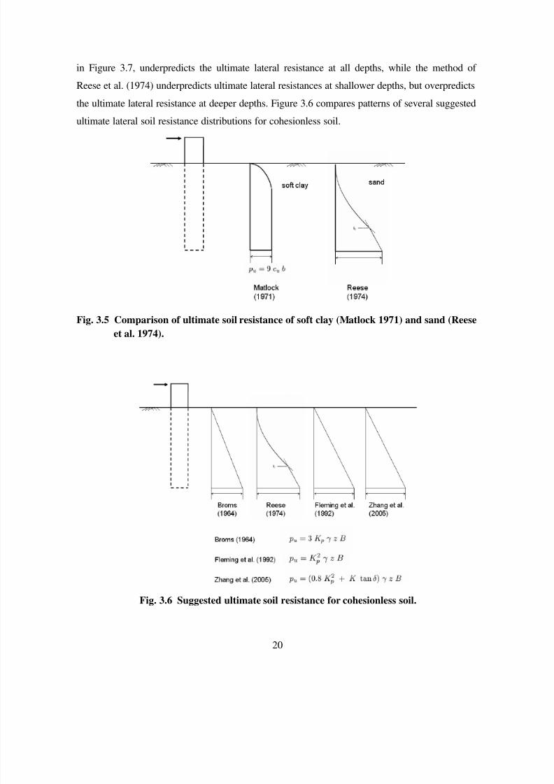
20
in Figure 3.7, underpredicts the ultimate lateral resistance at all depths, while the method of
Reese et al. (1974) underpredicts ultimate lateral resistances at shallower depths, but overpredicts
the ultimate lateral resistance at deeper depths. Figure 3.6 compares patterns of several suggested
ultimate lateral soil resistance distributions for cohesionless soil.
Fig. 3.5 Comparison of ultimate soil resistance of soft clay (Matlock 1971) and sand (Reese
et al. 1974).
Fig. 3.6 Suggested ultimate soil resistance for cohesionless soil.
7/21/2019 PEER807 KRAMERArduino Shin
http://slidepdf.com/reader/full/peer807-kramerarduino-shin 36/198
21
3.3.2 p-y Curves for Liquefiable Soil
In the previous subsection, conventional p-y curves were introduced. These curves were
developed mainly from experimental tests where the pile head was loaded monotonically or
cyclically. Since the applied loading rate was slow in most cases, there was no excess porewater
pressure built-up in the saturated soil around the pile. However, when a pile is subjected to
earthquake shaking, the soil around the pile may liquefy, if susceptible, and the soil resistance
may change due to porewater pressure generation. This is an important aspect, particularly for
deep foundations on liquefiable soils. In this section, recent studies on the lateral resistance of
piles in liquefiable soil are discussed.
3.3.2.1
Back -Calculated p-y Curves for Piles in L evel Ground Liquefiable Soils
When the soil around a pile is liquefied the soil resistance around the pile changes. To better
understand these changes several types of dynamic experiments have recently been performed
including: (i) centrifuge tests (Dobry et al. 1995; Wilson et al. 2000), (ii) large-scale laminar
shear box shaking tests (Tokimatsu et al. 2001), and (iii) full-scale field blasting tests (Rollins et
al. 2005; Weaver et al. 2005; Gerber and Rollins (2005).
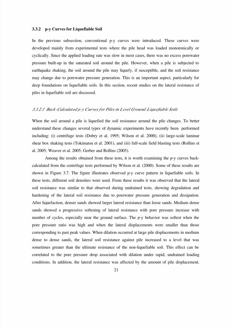
Among the results obtained from these tests, it is worth examining the p-y curves back-
calculated from the centrifuge tests performed by Wilson et al. (2000). Some of these results are
shown in Figure 3.7. The figure illustrates observed p-y curve pattern in liquefiable soils. In
these tests, different soil densities were used. From these results it was observed that the lateral
soil resistance was similar to that observed during undrained tests, showing degradation and
hardening of the lateral soil resistance due to porewater pressure generation and dissipation.
After liquefaction, denser sands showed larger lateral resistance than loose sands. Medium dense
sands showed a progressive softening of lateral resistance with pore pressure increase with
number of cycles, especially near the ground surface. The p-y behavior was softest when thepore pressure ratio was high and when the lateral displacements were smaller than those
corresponding to past peak values. When dilation occurred at large pile displacements in medium
dense to dense sands, the lateral soil resistance against pile increased to a level that was
sometimes greater than the ultimate resistance of the non-liquefiable soil. This effect can be
correlated to the pore pressure drop associated with dilation under rapid, undrained loading
conditions. In addition, the lateral resistance was affected by the amount of pile displacement,
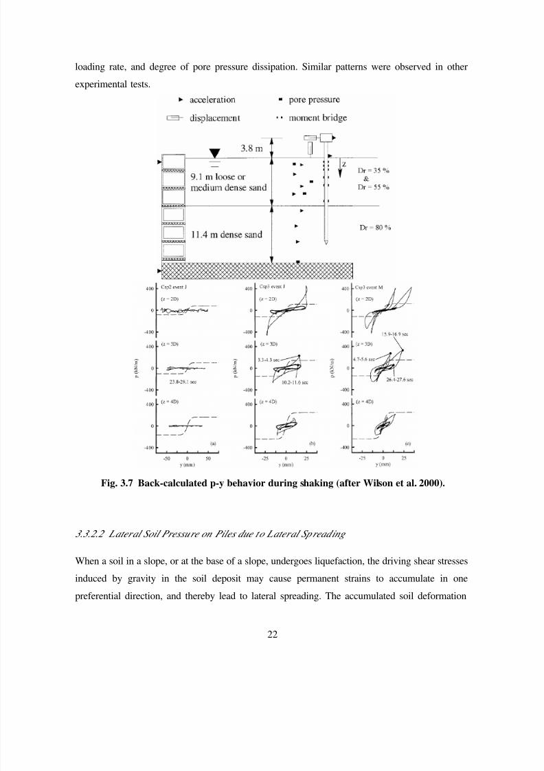
7/21/2019 PEER807 KRAMERArduino Shin
http://slidepdf.com/reader/full/peer807-kramerarduino-shin 37/198
22
loading rate, and degree of pore pressure dissipation. Similar patterns were observed in other
experimental tests.
Fig. 3.7 Back-calculated p-y behavior during shaking (after Wilson et al. 2000).
3.3.2.2 Lateral Soil Pressure on Piles due to Lateral Spreading
When a soil in a slope, or at the base of a slope, undergoes liquefaction, the driving shear stresses
induced by gravity in the soil deposit may cause permanent strains to accumulate in one
preferential direction, and thereby lead to lateral spreading. The accumulated soil deformation
7/21/2019 PEER807 KRAMERArduino Shin
http://slidepdf.com/reader/full/peer807-kramerarduino-shin 38/198
23
during shaking can induce large amounts of kinematic forces on the pile foundation, which may
result in severe damage to foundations and structures such as a bridges or port facilities.
To analyze piles subjected to lateral spreading, the lateral force induced by the liquefied
layer must be considered. This can be done assuming a constant pressure distribution
independent of the amount of soil displacement, or by using spring forces that depend on
imposed soil displacements. In both approaches, the lateral force applied to the pile depends on
the liquefied soil properties, distribution of soil displacement, and the velocity of the lateral flow
(Wang and Reese (1998). Among these factors, the strength of the liquefied soil is most
important.
To estimate the liquefiable soil resistance, the conventional soil resistance without
liquefaction is scaled by a p-multiplier that accounts for a simplified distribution of pore pressure
ratio along the pile. p-multipliers for fully liquefied soils vary depending on the test conditions
(Dobry et al. 1995; Wilson 1998). For example, the Japan Road Association (JRA 2002)
guidelines suggests a 30% of total overburden stress times pile diameter for the lateral pressure
imposed by the liquefiable soil with an additional reduction factor associated with the distance
from the waterfront.
Another way to estimate the kinematic load on the pile from lateral spreading is to
assume that the liquefied sand behaves as an undrained soil with a certain residual shear strength.
Among several ways to estimate the residual strength, the in-situ test approach is commonly
used. This method is based on correlations between SPT resistance and back-calculated shear
strengths from flow slide case histories (Seed 1986; Stark and Mesri 1992; Seed and Harder
1990). Figure 3.8 shows one of these correlations. Unfortunately, this approach includes
considerable uncertainties due to the variability of soil and stress conditions in the case histories.
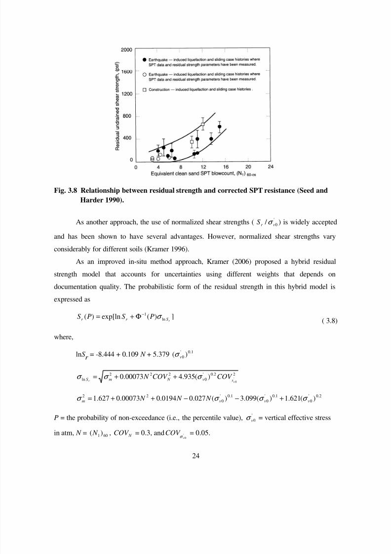
7/21/2019 PEER807 KRAMERArduino Shin
http://slidepdf.com/reader/full/peer807-kramerarduino-shin 39/198
24
Fig. 3.8 Relationship between residual strength and corrected SPT resistance (Seed and
Harder 1990).
As another approach, the use of normalized shear strengths ( '
0 / vr S σ ) is widely accepted
and has been shown to have several advantages. However, normalized shear strengths vary
considerably for different soils (Kramer 1996).
As an improved in-situ method approach, Kramer (2006) proposed a hybrid residual
strength model that accounts for uncertainties using different weights that depends ondocumentation quality. The probabilistic form of the residual strength in this hybrid model is
expressed as
])(exp[ln)( ln
1
r S r r PS PS σ −Φ+= ( 3.8)
where,
lnS r = -8.444 + 0.109 N + 5.379 1.0'
0 )( vσ
22.0'
0
222
ln '0
)(935.400073.0vr sv N mS COV COV N σ σ σ ++=
2.0'
0
1.0'
0
1.0'
0
22)(621.1)(099.3)(027.00194.000073.0627.1 vvvm N N N σ σ σ σ +−−++=
P = the probability of non-exceedance (i.e., the percentile value), '
0vσ = vertical effective stress
in atm, N = 601)( N , N COV = 0.3, and '0v
COV σ
= 0.05.
7/21/2019 PEER807 KRAMERArduino Shin
http://slidepdf.com/reader/full/peer807-kramerarduino-shin 40/198
25
3.3.2.3 Approximation of L iquefiable p-y Curves
As discussed previously, the lateral resistance of liquefiable soil against piles cannot be simply
defined using conventional p-y backbone envelopes. Moreover, the resistance is found to be
strongly correlated to the characteristics of the undrained soil behavior; which depends on
density, displacement history and displacement level, depth (i.e., confining pressure), and other
factors. Several researchers have tried to encapsulate these effects within the pore pressure ratio,
ur , and establish approximate p-y curves based on this parameter; since the pore pressure change
and phase transformation effects (contraction and dilation) governs the undrained soil behavior.
In this approximation, the lateral resistance is assumed to be inversely proportional to pore
pressure ratio ( ur ) in a degradation parameter (often also called p-multiplier).
Dobry et al. (1995) used this inverse relationship to capture the response observed in
centrifuge pseudo-static tests of single pile embedded in liquefiable leveled ground soil
( %40»r D ). Using measured pore pressure ratio distributions with depth to evaluate the
degradation of the p-y curves, pile bending moments were predicted reasonably well. Using a
similar approach, Wilson (1998) concluded that p-multipliers ranging from 0.1 to 0.2 for
Dr»40% and from 0.25 to 0.35 for Dr»55% in pseudo-static analysis give reasonable results for
representative peak loading cycles on a single pile. In a recent work Brandenberg (2005)
recommended more refined p-multiplier values to account for liquefaction effects in pseudo-
static analysis for different (N1)60-cs. These values are shown in Table 3.4.
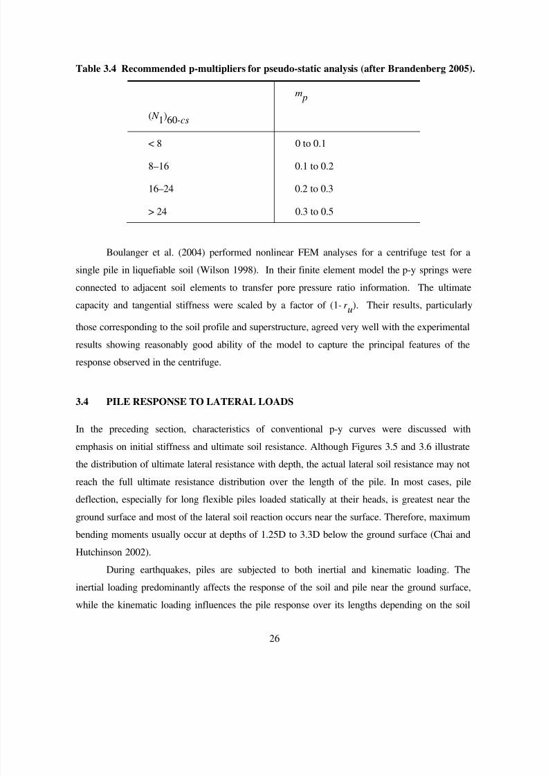
7/21/2019 PEER807 KRAMERArduino Shin
http://slidepdf.com/reader/full/peer807-kramerarduino-shin 41/198
26
Table 3.4 Recommended p-multipliers for pseudo-static analysis (after Brandenberg 2005).
( N 1)60-cs
m p
< 8 0 to 0.1
8–16 0.1 to 0.2
16–24 0.2 to 0.3
> 24 0.3 to 0.5
Boulanger et al. (2004) performed nonlinear FEM analyses for a centrifuge test for a
single pile in liquefiable soil (Wilson 1998). In their finite element model the p-y springs were
connected to adjacent soil elements to transfer pore pressure ratio information. The ultimate
capacity and tangential stiffness were scaled by a factor of (1-r u). Their results, particularly
those corresponding to the soil profile and superstructure, agreed very well with the experimental
results showing reasonably good ability of the model to capture the principal features of the
response observed in the centrifuge.
3.4 PILE RESPONSE TO LATERAL LOADS
In the preceding section, characteristics of conventional p-y curves were discussed with
emphasis on initial stiffness and ultimate soil resistance. Although Figures 3.5 and 3.6 illustrate
the distribution of ultimate lateral resistance with depth, the actual lateral soil resistance may not
reach the full ultimate resistance distribution over the length of the pile. In most cases, pile
deflection, especially for long flexible piles loaded statically at their heads, is greatest near the
ground surface and most of the lateral soil reaction occurs near the surface. Therefore, maximumbending moments usually occur at depths of 1.25D to 3.3D below the ground surface (Chai and
Hutchinson 2002).
During earthquakes, piles are subjected to both inertial and kinematic loading. The
inertial loading predominantly affects the response of the soil and pile near the ground surface,
while the kinematic loading influences the pile response over its lengths depending on the soil
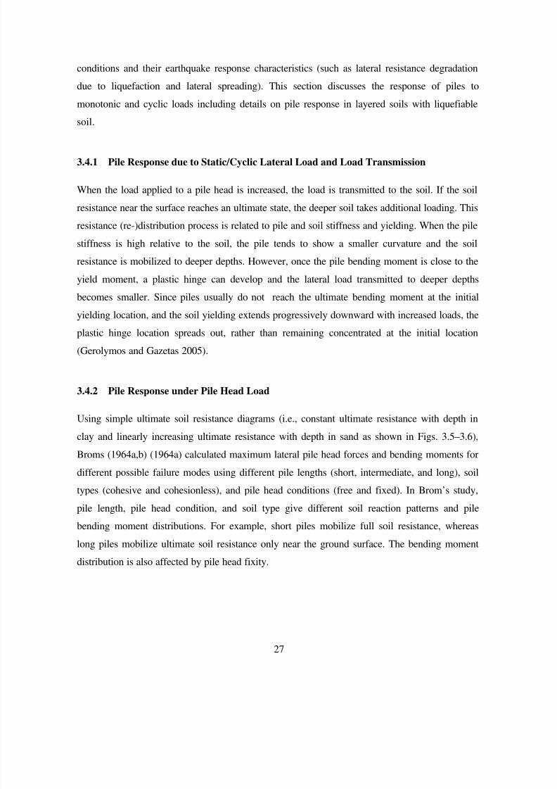
7/21/2019 PEER807 KRAMERArduino Shin
http://slidepdf.com/reader/full/peer807-kramerarduino-shin 42/198
27
conditions and their earthquake response characteristics (such as lateral resistance degradation
due to liquefaction and lateral spreading). This section discusses the response of piles to
monotonic and cyclic loads including details on pile response in layered soils with liquefiable
soil.
3.4.1 Pile Response due to Static/Cyclic Lateral Load and Load Transmission
When the load applied to a pile head is increased, the load is transmitted to the soil. If the soil
resistance near the surface reaches an ultimate state, the deeper soil takes additional loading. This
resistance (re-)distribution process is related to pile and soil stiffness and yielding. When the pile
stiffness is high relative to the soil, the pile tends to show a smaller curvature and the soil
resistance is mobilized to deeper depths. However, once the pile bending moment is close to theyield moment, a plastic hinge can develop and the lateral load transmitted to deeper depths
becomes smaller. Since piles usually do not reach the ultimate bending moment at the initial
yielding location, and the soil yielding extends progressively downward with increased loads, the
plastic hinge location spreads out, rather than remaining concentrated at the initial location
(Gerolymos and Gazetas 2005).
3.4.2 Pile Response under Pile Head Load
Using simple ultimate soil resistance diagrams (i.e., constant ultimate resistance with depth in
clay and linearly increasing ultimate resistance with depth in sand as shown in Figs. 3.5–3.6),
Broms (1964a,b) (1964a) calculated maximum lateral pile head forces and bending moments for
different possible failure modes using different pile lengths (short, intermediate, and long), soil
types (cohesive and cohesionless), and pile head conditions (free and fixed). In Brom’s study,
pile length, pile head condition, and soil type give different soil reaction patterns and pile
bending moment distributions. For example, short piles mobilize full soil resistance, whereas
long piles mobilize ultimate soil resistance only near the ground surface. The bending moment
distribution is also affected by pile head fixity.
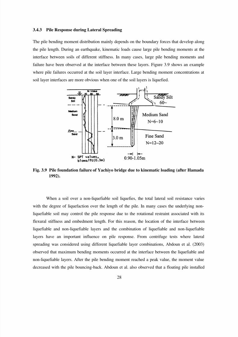
7/21/2019 PEER807 KRAMERArduino Shin
http://slidepdf.com/reader/full/peer807-kramerarduino-shin 43/198
28
3.4.3 Pile Response during Lateral Spreading
The pile bending moment distribution mainly depends on the boundary forces that develop along
the pile length. During an earthquake, kinematic loads cause large pile bending moments at the
interface between soils of different stiffness. In many cases, large pile bending moments and
failure have been observed at the interface between these layers. Figure 3.9 shows an example
where pile failures occurred at the soil layer interface. Large bending moment concentrations at
soil layer interfaces are more obvious when one of the soil layers is liquefied.
Fig. 3.9 Pile foundation failure of Yachiyo bridge due to kinematic loading (after Hamada
1992).
When a soil over a non-liquefiable soil liquefies, the total lateral soil resistance varies
with the degree of liquefaction over the length of the pile. In many cases the underlying non-
liquefiable soil may control the pile response due to the rotational restraint associated with its
flexural stiffness and embedment length. For this reason, the location of the interface between
liquefiable and non-liquefiable layers and the combination of liquefiable and non-liquefiable
layers have an important influence on pile response. From centrifuge tests where lateral
spreading was considered using different liquefiable layer combinations, Abdoun et al. (2003)
observed that maximum bending moments occurred at the interface between the liquefiable and
non-liquefiable layers. After the pile bending moment reached a peak value, the moment value
decreased with the pile bouncing-back. Abdoun et al. also observed that a floating pile installed
7/21/2019 PEER807 KRAMERArduino Shin
http://slidepdf.com/reader/full/peer807-kramerarduino-shin 44/198
29
in a non-liquefiable layer over a liquefiable layer had a maximum bending moment at the top of
the liquefiable layer since displacements at the upper non-liquefiable soil exceeded that of the
liquefied lower layer. In cases where piles were embedded in three layers (non-liquefiable layer
over liquefiable layer over a non-liquefiable layer), large maximum bending moments occurred
at the layer interfaces (i.e., at the top and bottom of the liquefiable layer) although the larger
maximum values occurred at the lower interface. In these cases, it was also observed that the
measured bending moment distribution within the liquefied layer was nearly linear showing little
contribution to the pile bending moment from the liquefied soil. Another observation was that
soil densification due to pile driving resulted in larger bending moments than those in cast-in-
place piles due to the fact that the densification increased the initial effective stress, and hence
the stiffness of the soil surrounding the pile.
3.5 PILE GROUP RESPONSE TO LATERAL LOADS
Pile groups consist of rows of piles whose heads are connected by a rigid pile cap. The lateral
capacity of pile groups depends on the individual pile capacities, pile spacing, pile installation
method, pile cap resistance, and other factors.
3.5.1 Group Effect
The efficiency of an individual pile in a pile group (compared to a single isolated pile) depends
primarily on pile spacing, alignment, and location within the group. When piles in a group are
closely spaced, lateral pile movements affect the stresses in the soil around the adjacent piles.
Figure 3.10 shows two possible pile alignments: in-line and side-by-side. In in-line alignments, a
front pile (or leading pile) takes more load than the others and the rear pile (trailing pile)
mobilizes less soil resistance. This effect is referred to as the shadow effect. In side-by-side
alignments, corner piles located at the corner or at the edge of a pile group take a greater share of
the load than the interior piles. This is particularly noticeable when piles are closely spaced. This
effect is referred to as the edge effect.
7/21/2019 PEER807 KRAMERArduino Shin
http://slidepdf.com/reader/full/peer807-kramerarduino-shin 45/198
30
Fig. 3.10 Schematic of pile alignment in group.
To capture the response of piles in a pile group, group efficiency factors are included in
the p-y curves using p-multipliers (Brown et al. 1988). To evaluate these p-multipliers several
researchers have performed experimental tests on pile groups using different pile group sizes
(i.e., number of rows and piles per row), pile spacing, pile cap rotational conditions, and soil type
and density. Mokwa (1999) studied pile group behavior and pile cap resistance and completed a
comprehensive literature review using 350 journal articles and other publications, including 37
experimental studies (15 full-scale tests, 16 1-g model tests, and 6 centrifuge tests) andapproximately 30 analytical studies. Based on these studies, he concluded that pile spacing is the
dominant factor affecting pile group response and that group effects are negligible when the
center-to-center pile spacing is greater than 6D in in-line configurations or greater than 3D in the
side-by-side configurations. He also concluded that soil type and density does not affect
significantly the pile group efficiency, and that efficiency decreases with increasing displacement
and becomes constant after a deformation of 5% of pile diameter. He also developed
relationships to estimate pile group efficiencies and p-multipliers as a function of pile
arrangement and pile spacing. Figure 3.11 shows Mokwa’s p-multipliers for leading and trailing
rows. Other group efficiency values versus pile spacing for different pile alignments in a pile
group can be found in Mokwa (1999).
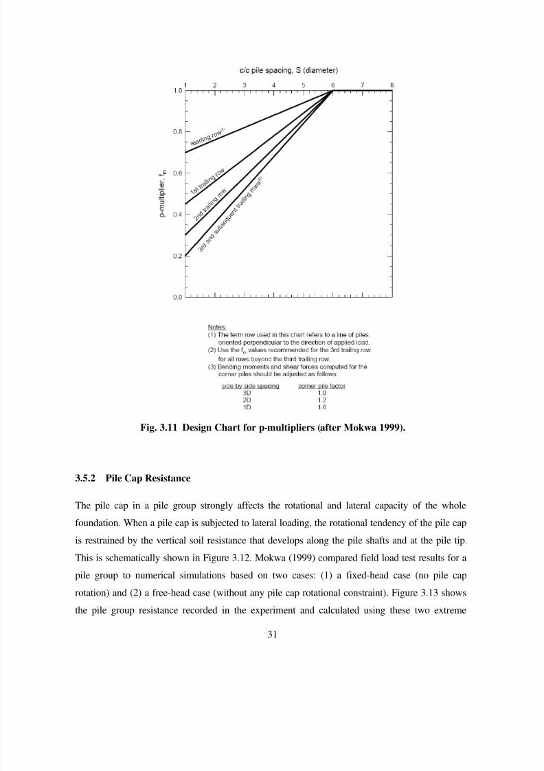
7/21/2019 PEER807 KRAMERArduino Shin
http://slidepdf.com/reader/full/peer807-kramerarduino-shin 46/198
31
Fig. 3.11 Design Chart for p-multipliers (after Mokwa 1999).
3.5.2 Pile Cap Resistance
The pile cap in a pile group strongly affects the rotational and lateral capacity of the whole
foundation. When a pile cap is subjected to lateral loading, the rotational tendency of the pile cap
is restrained by the vertical soil resistance that develops along the pile shafts and at the pile tip.
This is schematically shown in Figure 3.12. Mokwa (1999) compared field load test results for a
pile group to numerical simulations based on two cases: (1) a fixed-head case (no pile cap
rotation) and (2) a free-head case (without any pile cap rotational constraint). Figure 3.13 shows
the pile group resistance recorded in the experiment and calculated using these two extreme
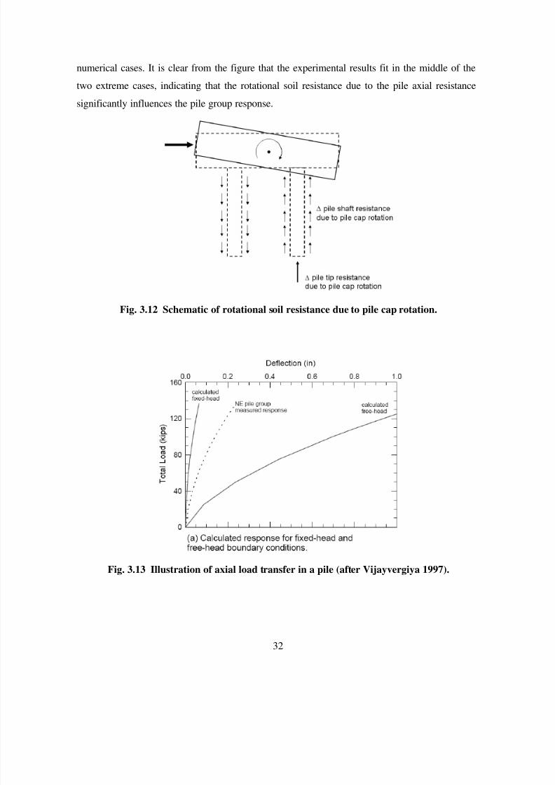
7/21/2019 PEER807 KRAMERArduino Shin
http://slidepdf.com/reader/full/peer807-kramerarduino-shin 47/198
32
numerical cases. It is clear from the figure that the experimental results fit in the middle of the
two extreme cases, indicating that the rotational soil resistance due to the pile axial resistance
significantly influences the pile group response.
Fig. 3.12 Schematic of rotational soil resistance due to pile cap rotation.
Fig. 3.13 Illustration of axial load transfer in a pile (after Vijayvergiya 1997).
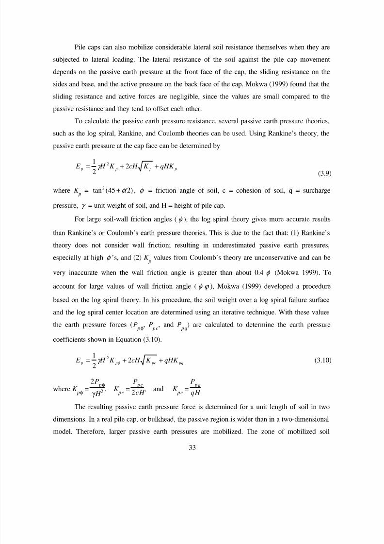
7/21/2019 PEER807 KRAMERArduino Shin
http://slidepdf.com/reader/full/peer807-kramerarduino-shin 48/198
33
Pile caps can also mobilize considerable lateral soil resistance themselves when they are
subjected to lateral loading. The lateral resistance of the soil against the pile cap movement
depends on the passive earth pressure at the front face of the cap, the sliding resistance on the
sides and base, and the active pressure on the back face of the cap. Mokwa (1999) found that the
sliding resistance and active forces are negligible, since the values are small compared to the
passive resistance and they tend to offset each other.
To calculate the passive earth pressure resistance, several passive earth pressure theories,
such as the log spiral, Rankine, and Coulomb theories can be used. Using Rankine’s theory, the
passive earth pressure at the cap face can be determined by
p p p p qHK K cH K H E ++= 22
1 2γ (3.9)
where K p
= /2)+ φ 45(tan2 , φ = friction angle of soil, c = cohesion of soil, q = surcharge
pressure, γ = unit weight of soil, and H = height of pile cap.
For large soil-wall friction angles ( φ ), the log spiral theory gives more accurate results
than Rankine’s or Coulomb’s earth pressure theories. This is due to the fact that: (1) Rankine’s
theory does not consider wall friction; resulting in underestimated passive earth pressures,
especially at high φ ’s, and (2) K p
values from Coulomb’s theory are unconservative and can be
very inaccurate when the wall friction angle is greater than about 0.4 φ (Mokwa 1999). To
account for large values of wall friction angle ( φ ϕ ), Mokwa (1999) developed a procedure
based on the log spiral theory. In his procedure, the soil weight over a log spiral failure surface
and the log spiral center location are determined using an iterative technique. With these values
the earth pressure forces (P p φ
, P p c
, and P p q
) are calculated to determine the earth pressure
coefficients shown in Equation (3.10).
pq pc p pqHK K cH K H E
++= 22
1 2
φ γ (3.10)
where K p φ
=2 P
p φ
γ H 2, K
p c =
P p c
2 c H , and K
p c =
P p q
q H
The resulting passive earth pressure force is determined for a unit length of soil in two
dimensions. In a real pile cap, or bulkhead, the passive region is wider than in a two-dimensional
model. Therefore, larger passive earth pressures are mobilized. The zone of mobilized soil
7/21/2019 PEER807 KRAMERArduino Shin
http://slidepdf.com/reader/full/peer807-kramerarduino-shin 49/198
34
resistance depends on the friction angle of the soil and on depth. To include the three-
dimensional pile cap effect, Mokwa (1999) performed field load tests on bulkheads and
measured the pure pile cap lateral resistance without the lateral resistance of the piles. Mokwa
found that using log spiral theory, together with Oveson’s (Ovesen 1964) three-dimensional
shape factors, accurate results were obtained for both c-φ natural soils and cohesionless crusher
run backfill. Ovesen (1964) introduced a 3-D modifying factor (R) expressed by
+
−+
+
+−+=
H
b
B E K K
H
b
B E K K R
a p
a p
05.01
)(4.0
51
6.11.1)(1
23
43 / 2
(3.11)
where B = 1 for a single pile cap or anchor block, E = 1 -
H
z+ H , and z is embedment depth from
the ground surface to the top of the pile cap.
For cohesionless soil, the ultimate earth pressure force, accounting for the 3-D effect, can
be expressed by
bPPP Rb RE P pq pc p pcapult ++== φ . (3.12)
where R is Ovesen’s 3-D modifying factor calculated from Equation (3.11), E p
is the 2-D passive
earth pressure obtained using Equation (3.10), and b is pile cap width.
For cohesive soils (φ = 0), Mokwa (1999) suggested the so-called φ =0 sliding wedge
method to calculate passive earth pressure. The method follows Reese’s sliding surface wedge
approach for a laterally loaded pile and is based on full-scale test results. Equation (3.13) shows
a semi-empirical equation for the ultimate passive earth pressure for cohesive soils
+++= α
γ 2
25.04
2,
b
H
c
H cbH P capult (3.13)
where α is a factor that accounts for adhesion between the cohesive soil and the wall. Table 3.5
shows typical values for α. Since the three-dimensional and shape effects are implicitly included
in the experimental tests, no additional modification factors are needed.
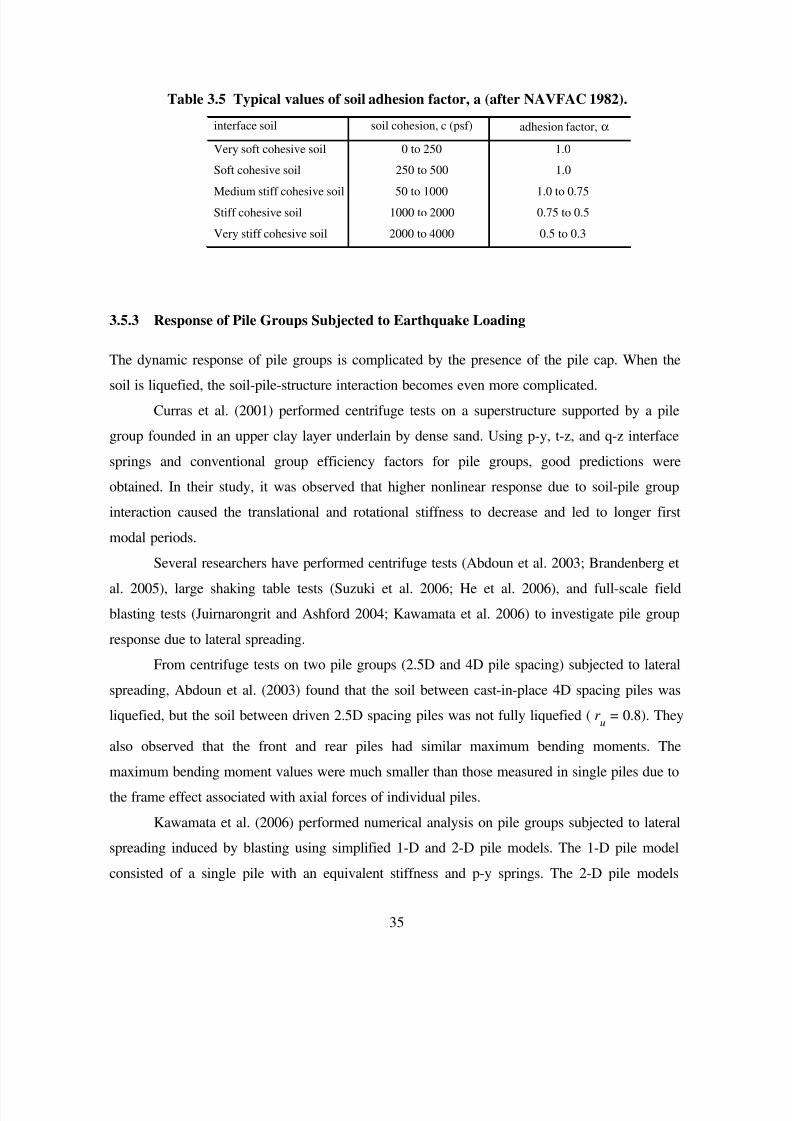
7/21/2019 PEER807 KRAMERArduino Shin
http://slidepdf.com/reader/full/peer807-kramerarduino-shin 50/198
35
Table 3.5 Typical values of soil adhesion factor, a (after NAVFAC 1982).
interface soil soil cohesion, c (psf) adhesion factor, α
Very soft cohesive soil 0 to 250 1.0
Soft cohesive soil 250 to 500 1.0
Medium stiff cohesive soil 50 to 1000 1.0 to 0.75
Stiff cohesive soil 1000 to 2000 0.75 to 0.5
Very stiff cohesive soil 2000 to 4000 0.5 to 0.3
3.5.3 Response of Pile Groups Subjected to Earthquake Loading
The dynamic response of pile groups is complicated by the presence of the pile cap. When the
soil is liquefied, the soil-pile-structure interaction becomes even more complicated.
Curras et al. (2001) performed centrifuge tests on a superstructure supported by a pile
group founded in an upper clay layer underlain by dense sand. Using p-y, t-z, and q-z interface
springs and conventional group efficiency factors for pile groups, good predictions were
obtained. In their study, it was observed that higher nonlinear response due to soil-pile group
interaction caused the translational and rotational stiffness to decrease and led to longer first
modal periods.
Several researchers have performed centrifuge tests (Abdoun et al. 2003; Brandenberg et
al. 2005), large shaking table tests (Suzuki et al. 2006; He et al. 2006), and full-scale field
blasting tests (Juirnarongrit and Ashford 2004; Kawamata et al. 2006) to investigate pile group
response due to lateral spreading.
From centrifuge tests on two pile groups (2.5D and 4D pile spacing) subjected to lateral
spreading, Abdoun et al. (2003) found that the soil between cast-in-place 4D spacing piles was
liquefied, but the soil between driven 2.5D spacing piles was not fully liquefied (r u = 0.8). They
also observed that the front and rear piles had similar maximum bending moments. Themaximum bending moment values were much smaller than those measured in single piles due to
the frame effect associated with axial forces of individual piles.
Kawamata et al. (2006) performed numerical analysis on pile groups subjected to lateral
spreading induced by blasting using simplified 1-D and 2-D pile models. The 1-D pile model
consisted of a single pile with an equivalent stiffness and p-y springs. The 2-D pile models
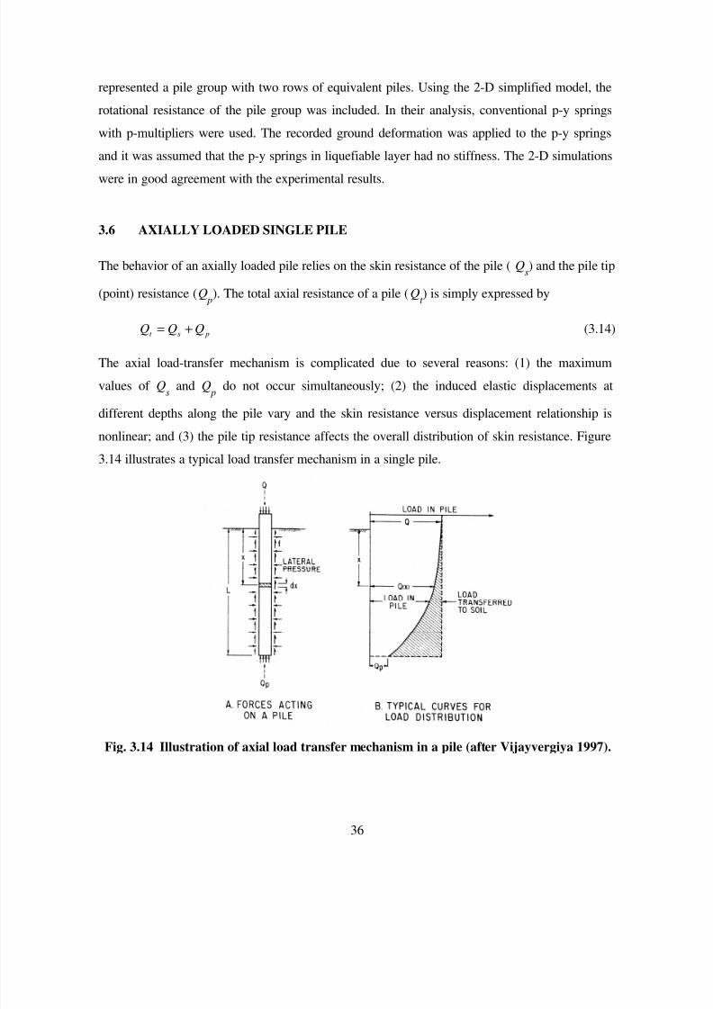
7/21/2019 PEER807 KRAMERArduino Shin
http://slidepdf.com/reader/full/peer807-kramerarduino-shin 51/198
36
represented a pile group with two rows of equivalent piles. Using the 2-D simplified model, the
rotational resistance of the pile group was included. In their analysis, conventional p-y springs
with p-multipliers were used. The recorded ground deformation was applied to the p-y springs
and it was assumed that the p-y springs in liquefiable layer had no stiffness. The 2-D simulations
were in good agreement with the experimental results.
3.6 AXIALLY LOADED SINGLE PILE
The behavior of an axially loaded pile relies on the skin resistance of the pile ( Qs) and the pile tip
(point) resistance (Q p
). The total axial resistance of a pile (Qt ) is simply expressed by
pst
QQQ += (3.14)
The axial load-transfer mechanism is complicated due to several reasons: (1) the maximum
values of Qs and Q
p do not occur simultaneously; (2) the induced elastic displacements at
different depths along the pile vary and the skin resistance versus displacement relationship is
nonlinear; and (3) the pile tip resistance affects the overall distribution of skin resistance. Figure
3.14 illustrates a typical load transfer mechanism in a single pile.
Fig. 3.14 Illustration of axial load transfer mechanism in a pile (after Vijayvergiya 1997).
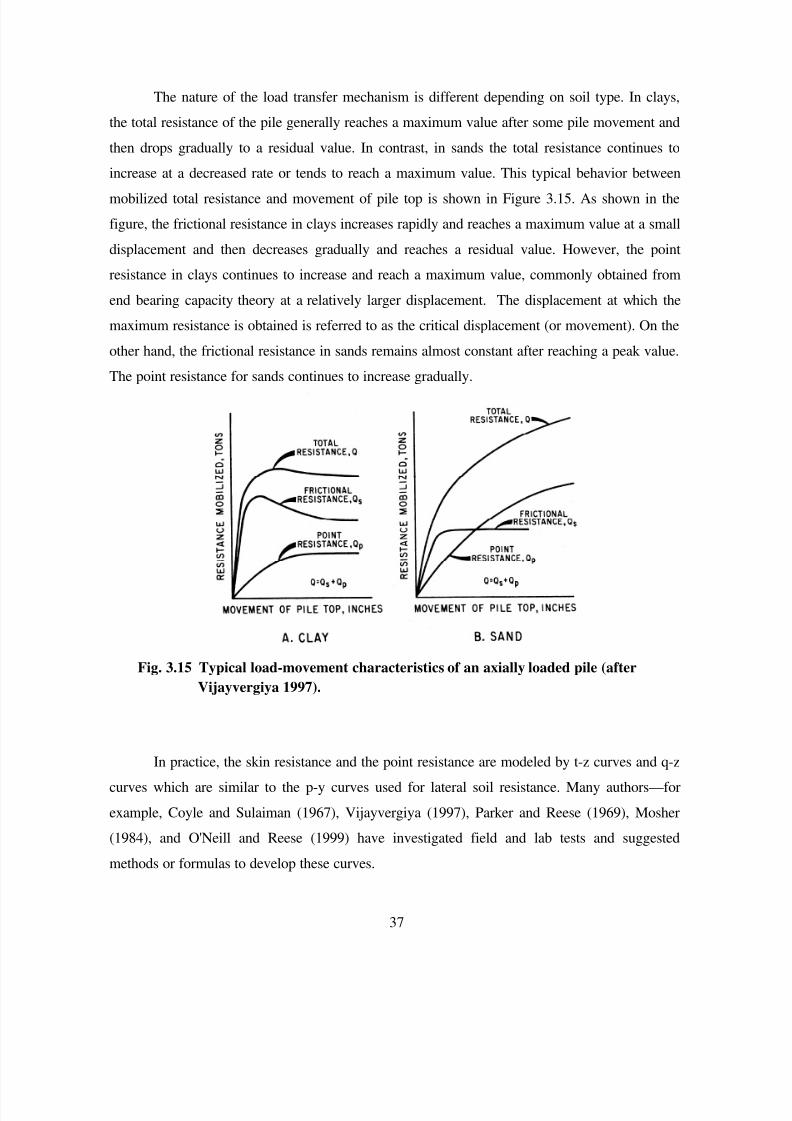
7/21/2019 PEER807 KRAMERArduino Shin
http://slidepdf.com/reader/full/peer807-kramerarduino-shin 52/198
37
The nature of the load transfer mechanism is different depending on soil type. In clays,
the total resistance of the pile generally reaches a maximum value after some pile movement and
then drops gradually to a residual value. In contrast, in sands the total resistance continues to
increase at a decreased rate or tends to reach a maximum value. This typical behavior between
mobilized total resistance and movement of pile top is shown in Figure 3.15. As shown in the
figure, the frictional resistance in clays increases rapidly and reaches a maximum value at a small
displacement and then decreases gradually and reaches a residual value. However, the point
resistance in clays continues to increase and reach a maximum value, commonly obtained from
end bearing capacity theory at a relatively larger displacement. The displacement at which the
maximum resistance is obtained is referred to as the critical displacement (or movement). On the
other hand, the frictional resistance in sands remains almost constant after reaching a peak value.
The point resistance for sands continues to increase gradually.
Fig. 3.15 Typical load-movement characteristics of an axially loaded pile (after
Vijayvergiya 1997).
In practice, the skin resistance and the point resistance are modeled by t-z curves and q-z
curves which are similar to the p-y curves used for lateral soil resistance. Many authors—for
example, Coyle and Sulaiman (1967), Vijayvergiya (1997), Parker and Reese (1969), Mosher
(1984), and O'Neill and Reese (1999) have investigated field and lab tests and suggested
methods or formulas to develop these curves.
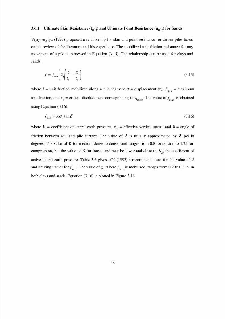
7/21/2019 PEER807 KRAMERArduino Shin
http://slidepdf.com/reader/full/peer807-kramerarduino-shin 53/198
38
3.6.1 Ultimate Skin Resistance (tult) and Ultimate Point Resistance (qult) for Sands
Vijayvergiya (1997) proposed a relationship for skin and point resistance for driven piles based
on his review of the literature and his experience. The mobilized unit friction resistance for any
movement of a pile is expressed in Equation (3.15). The relationship can be used for clays and
sands.
−=
cc z
z
z
z f f 2max (3.15)
where f = unit friction mobilized along a pile segment at a displacement (z), f max
= maximum
unit friction, and zc = critical displacement corresponding to q
max. The value of f
max is obtained
using Equation (3.16).
δ σ tanmax vK f = (3.16)
where K = coefficient of lateral earth pressure, σv = effective vertical stress, and δ = angle of
friction between soil and pile surface. The value of δ is usually approximated by δ=φ-5 in
degrees. The value of K for medium dense to dense sand ranges from 0.8 for tension to 1.25 for
compression, but the value of K for loose sand may be lower and close to K a, the coefficient of
active lateral earth pressure. Table 3.6 gives API (1993)’s recommendations for the value of δ
and limiting values for f max
. The value of zc, where f
max is mobilized, ranges from 0.2 to 0.3 in. in
both clays and sands. Equation (3.16) is plotted in Figure 3.16.
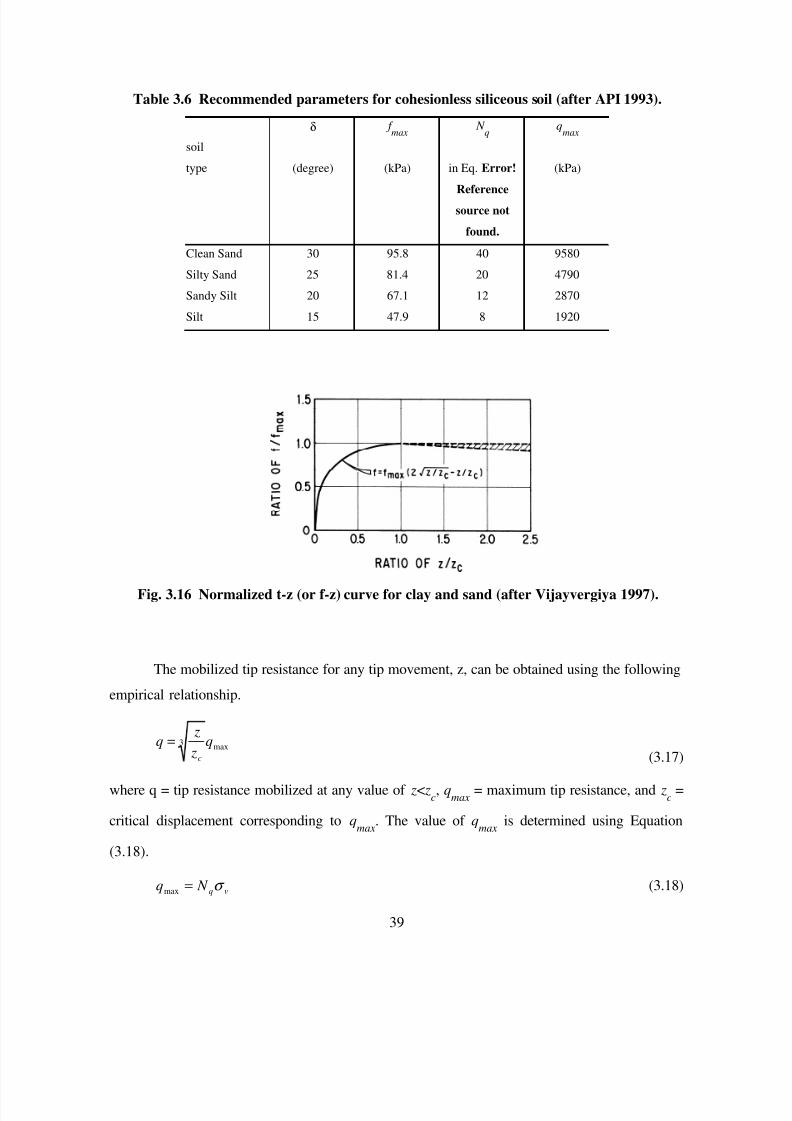
7/21/2019 PEER807 KRAMERArduino Shin
http://slidepdf.com/reader/full/peer807-kramerarduino-shin 54/198
39
Table 3.6 Recommended parameters for cohesionless siliceous soil (after API 1993).
soil
δ f max
N q q
max
type (degree) (kPa) in Eq. Error!
Reference
source not
found.
(kPa)
Clean Sand 30 95.8 40 9580
Silty Sand 25 81.4 20 4790
Sandy Silt 20 67.1 12 2870
Silt 15 47.9 8 1920
Fig. 3.16 Normalized t-z (or f-z) curve for clay and sand (after Vijayvergiya 1997).
The mobilized tip resistance for any tip movement, z, can be obtained using the following
empirical relationship.
max
3 q z
zq
c
= (3.17)
where q = tip resistance mobilized at any value of z< zc, q
max = maximum tip resistance, and z
c =
critical displacement corresponding to qmax
. The value of qmax
is determined using Equation
(3.18).
vq N q σ =max (3.18)
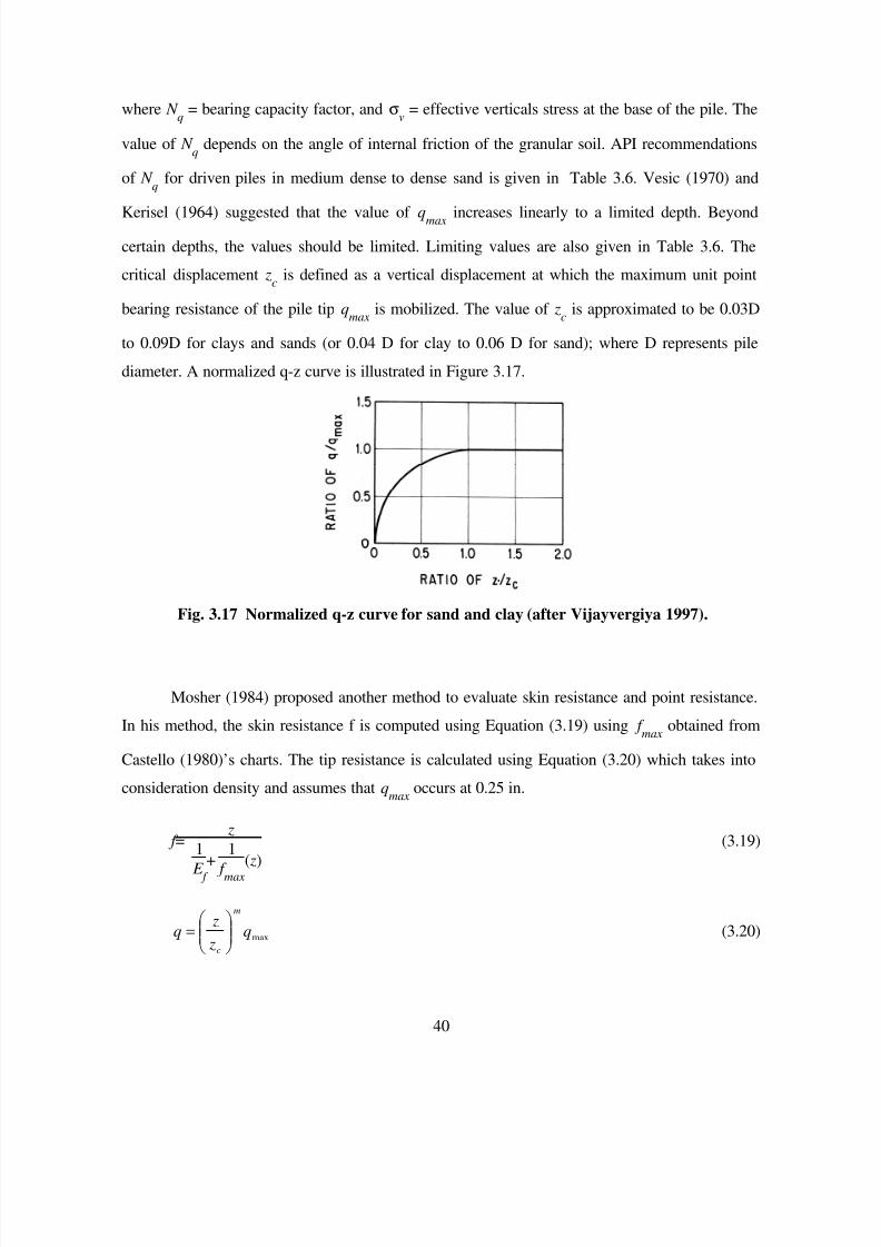
7/21/2019 PEER807 KRAMERArduino Shin
http://slidepdf.com/reader/full/peer807-kramerarduino-shin 55/198
40
where N q = bearing capacity factor, and σ
v = effective verticals stress at the base of the pile. The
value of N q depends on the angle of internal friction of the granular soil. API recommendations
of N q for driven piles in medium dense to dense sand is given in Table 3.6. Vesic (1970) and
Kerisel (1964) suggested that the value of qmax increases linearly to a limited depth. Beyond
certain depths, the values should be limited. Limiting values are also given in Table 3.6. The
critical displacement zc is defined as a vertical displacement at which the maximum unit point
bearing resistance of the pile tip qmax
is mobilized. The value of zc is approximated to be 0.03D
to 0.09D for clays and sands (or 0.04 D for clay to 0.06 D for sand); where D represents pile
diameter. A normalized q-z curve is illustrated in Figure 3.17.
Fig. 3.17 Normalized q-z curve for sand and clay (after Vijayvergiya 1997).
Mosher (1984) proposed another method to evaluate skin resistance and point resistance.
In his method, the skin resistance f is computed using Equation (3.19) using f max
obtained from
Castello (1980)’s charts. The tip resistance is calculated using Equation (3.20) which takes into
consideration density and assumes that qmax
occurs at 0.25 in.
f = z
1
E f
+1
f max
( z)
(3.19)
maxq z
zq
m
c
= (3.20)
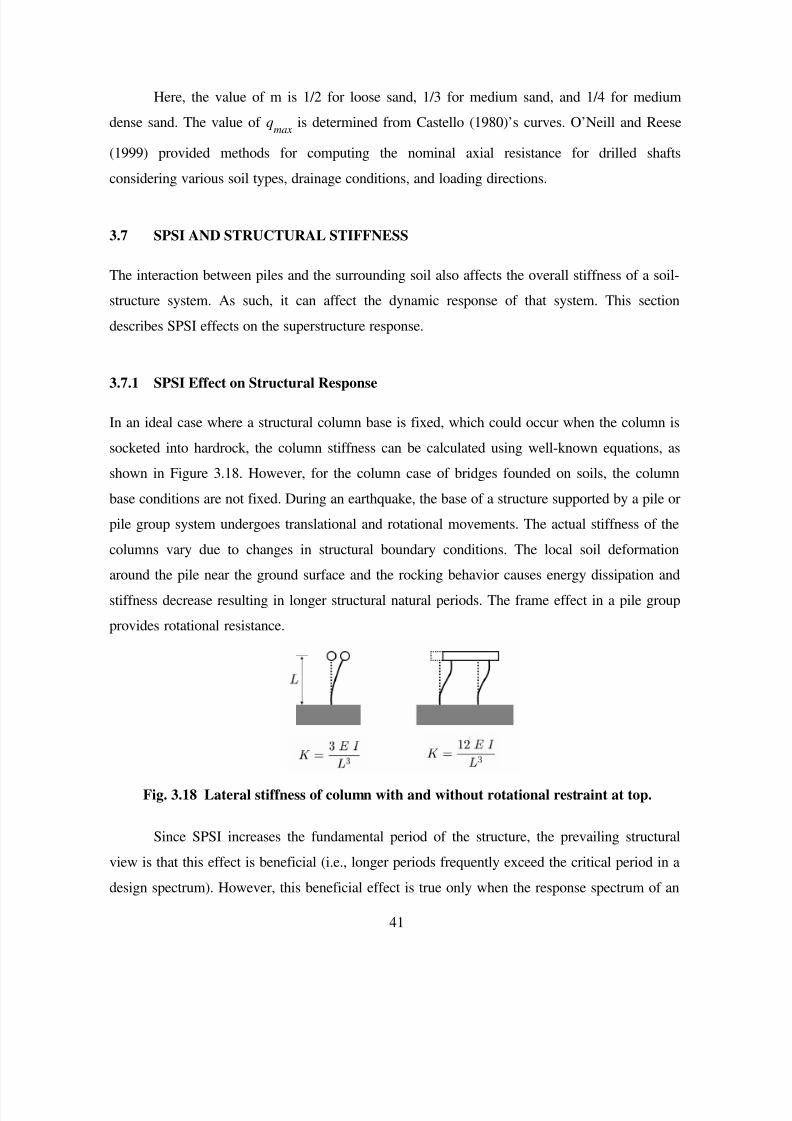
7/21/2019 PEER807 KRAMERArduino Shin
http://slidepdf.com/reader/full/peer807-kramerarduino-shin 56/198
41
Here, the value of m is 1/2 for loose sand, 1/3 for medium sand, and 1/4 for medium
dense sand. The value of qmax
is determined from Castello (1980)’s curves. O’Neill and Reese
(1999) provided methods for computing the nominal axial resistance for drilled shafts
considering various soil types, drainage conditions, and loading directions.
3.7 SPSI AND STRUCTURAL STIFFNESS
The interaction between piles and the surrounding soil also affects the overall stiffness of a soil-
structure system. As such, it can affect the dynamic response of that system. This section
describes SPSI effects on the superstructure response.
3.7.1 SPSI Effect on Structural Response
In an ideal case where a structural column base is fixed, which could occur when the column is
socketed into hardrock, the column stiffness can be calculated using well-known equations, as
shown in Figure 3.18. However, for the column case of bridges founded on soils, the column
base conditions are not fixed. During an earthquake, the base of a structure supported by a pile or
pile group system undergoes translational and rotational movements. The actual stiffness of the
columns vary due to changes in structural boundary conditions. The local soil deformation
around the pile near the ground surface and the rocking behavior causes energy dissipation and
stiffness decrease resulting in longer structural natural periods. The frame effect in a pile group
provides rotational resistance.
Fig. 3.18 Lateral stiffness of column with and without rotational restraint at top.
Since SPSI increases the fundamental period of the structure, the prevailing structural
view is that this effect is beneficial (i.e., longer periods frequently exceed the critical period in a
design spectrum). However, this beneficial effect is true only when the response spectrum of an
7/21/2019 PEER807 KRAMERArduino Shin
http://slidepdf.com/reader/full/peer807-kramerarduino-shin 57/198
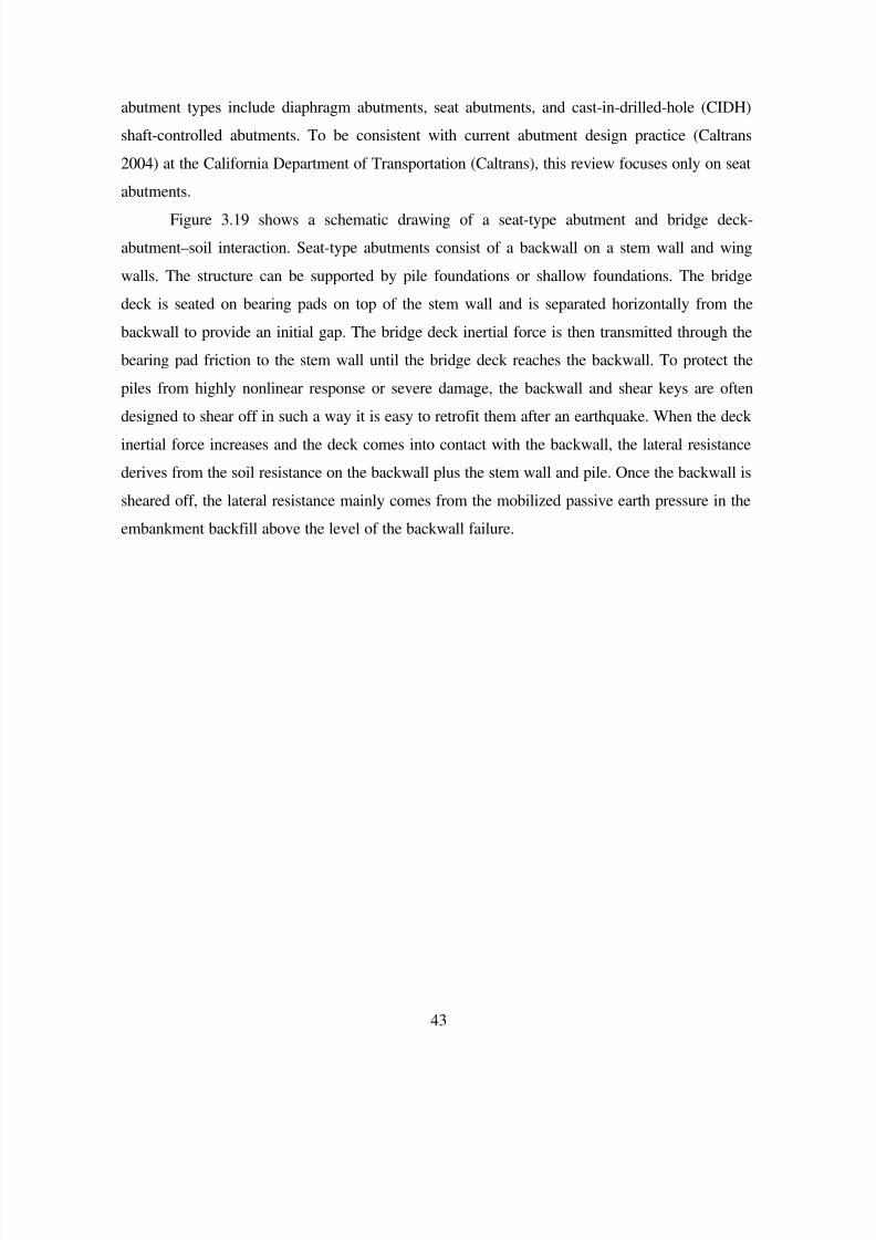
7/21/2019 PEER807 KRAMERArduino Shin
http://slidepdf.com/reader/full/peer807-kramerarduino-shin 58/198
43
abutment types include diaphragm abutments, seat abutments, and cast-in-drilled-hole (CIDH)
shaft-controlled abutments. To be consistent with current abutment design practice (Caltrans
2004) at the California Department of Transportation (Caltrans), this review focuses only on seat
abutments.
Figure 3.19 shows a schematic drawing of a seat-type abutment and bridge deck-
abutment–soil interaction. Seat-type abutments consist of a backwall on a stem wall and wing
walls. The structure can be supported by pile foundations or shallow foundations. The bridge
deck is seated on bearing pads on top of the stem wall and is separated horizontally from the
backwall to provide an initial gap. The bridge deck inertial force is then transmitted through the
bearing pad friction to the stem wall until the bridge deck reaches the backwall. To protect the
piles from highly nonlinear response or severe damage, the backwall and shear keys are often
designed to shear off in such a way it is easy to retrofit them after an earthquake. When the deck
inertial force increases and the deck comes into contact with the backwall, the lateral resistance
derives from the soil resistance on the backwall plus the stem wall and pile. Once the backwall is
sheared off, the lateral resistance mainly comes from the mobilized passive earth pressure in the
embankment backfill above the level of the backwall failure.
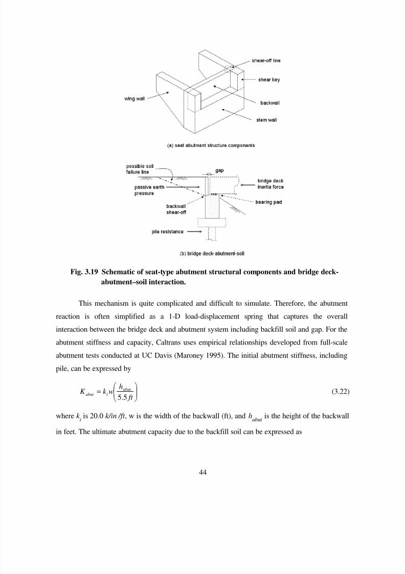
7/21/2019 PEER807 KRAMERArduino Shin
http://slidepdf.com/reader/full/peer807-kramerarduino-shin 59/198
44
Fig. 3.19 Schematic of seat-type abutment structural components and bridge deck-
abutment–soil interaction.
This mechanism is quite complicated and difficult to simulate. Therefore, the abutment
reaction is often simplified as a 1-D load-displacement spring that captures the overall
interaction between the bridge deck and abutment system including backfill soil and gap. For the
abutment stiffness and capacity, Caltrans uses empirical relationships developed from full-scale
abutment tests conducted at UC Davis (Maroney 1995). The initial abutment stiffness, including
pile, can be expressed by
5.5
= ft
hwk K abut
iabut (3.22)
where k i is 20.0 k/in /ft , w is the width of the backwall (ft), and h
abut is the height of the backwall
in feet. The ultimate abutment capacity due to the backfill soil can be expressed as
7/21/2019 PEER807 KRAMERArduino Shin
http://slidepdf.com/reader/full/peer807-kramerarduino-shin 60/198
45
××=
ft
hksf AP abut
eabut 5.5
)0.5( (3.23)
where Ae = the effective abutment area in ft2. The coefficient (5.0 ksf) is intended to account for
the static shear strength of a typical embankment material. Using the initial stiffness and ultimate
capacity, a 1-D load-displacement curve can be approximated using a simple curve as shown in
Figure 3.20.
Fig. 3.20 Simplified abutment load-deflection characteristic using initial stiffness and
ultimate resistance in Caltrans’s guideline (after SDC 2004).
3.9 SUMMARY
This chapter reviewed soil-structure interaction effects in bridge components with a focus on the
interface spring characteristics of piles and pile groups in various soil and loading conditions,
such as sands, clays, and liquefiable soils subjected to static and dynamic loading. The soil-pile
system response subjected to lateral spreading and factors that can influence the dynamic
response characteristics of pile-supported structures were reviewed. Finally, the soil-abutment
interaction was briefly discussed.
7/21/2019 PEER807 KRAMERArduino Shin
http://slidepdf.com/reader/full/peer807-kramerarduino-shin 61/198
4 Characteristics of Testbed Highway Bridge
4.1 INTRODUCTION
For reliable estimation of bridge performance, especially when subjected to liquefaction and
lateral spreading, appropriate modeling of soil-structure interaction and understanding of the
global bridge behavior are essential. In practice, soil and foundation systems are often
approximated using very simple foundation springs or unrealistic lateral spreading mechanisms
that may not represent all important aspects of the global system behavior. In this context, a
detailed bridge model in liquefiable soils was developed, putting emphasis on an accurate
modeling of both the structural and soil behavior including various SPSI modeling strategies for
several bridge system components such as pile, pile cap, and abutment wall structure. This model
was used to apply the PEER Performance-Based Earthquake engineering (PBEE) framework
described in Chapter 2.
4.2 TESTBED BRIDGE SYSTEM
This study considered a typical Caltrans highway bridge underlain by liquefiable soils
susceptible to lateral spreading. The superstructure of the five-span bridge is identical to that of
Stojadinović and Mackie (2007) who studied its performance assuming fixed-base conditions. In
this project, the bridge is supported on pile foundations that extend through a profile with loose,
saturated sandy soils that are susceptible to liquefaction and lateral spreading. A schematic
layout of the bridge is shown in Figure 4.1.
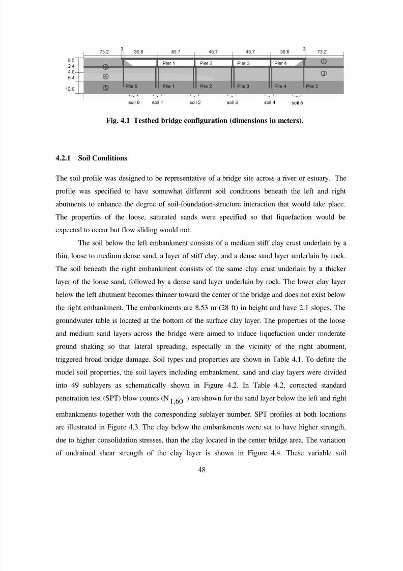
7/21/2019 PEER807 KRAMERArduino Shin
http://slidepdf.com/reader/full/peer807-kramerarduino-shin 62/198
48
Fig. 4.1 Testbed bridge configuration (dimensions in meters).
4.2.1 Soil Conditions
The soil profile was designed to be representative of a bridge site across a river or estuary. The
profile was specified to have somewhat different soil conditions beneath the left and right
abutments to enhance the degree of soil-foundation-structure interaction that would take place.
The properties of the loose, saturated sands were specified so that liquefaction would be
expected to occur but flow sliding would not.
The soil below the left embankment consists of a medium stiff clay crust underlain by a
thin, loose to medium dense sand, a layer of stiff clay, and a dense sand layer underlain by rock.
The soil beneath the right embankment consists of the same clay crust underlain by a thicker
layer of the loose sand, followed by a dense sand layer underlain by rock. The lower clay layer
below the left abutment becomes thinner toward the center of the bridge and does not exist below
the right embankment. The embankments are 8.53 m (28 ft) in height and have 2:1 slopes. The
groundwater table is located at the bottom of the surface clay layer. The properties of the loose
and medium sand layers across the bridge were aimed to induce liquefaction under moderate
ground shaking so that lateral spreading, especially in the vicinity of the right abutment,
triggered broad bridge damage. Soil types and properties are shown in Table 4.1. To define the
model soil properties, the soil layers including embankment, sand and clay layers were divided
into 49 sublayers as schematically shown in Figure 4.2. In Table 4.2, corrected standard
penetration test (SPT) blow counts (N1,60 ) are shown for the sand layer below the left and right
embankments together with the corresponding sublayer number. SPT profiles at both locations
are illustrated in Figure 4.3. The clay below the embankments were set to have higher strength,
due to higher consolidation stresses, than the clay located in the center bridge area. The variation
of undrained shear strength of the clay layer is shown in Figure 4.4. These variable soil
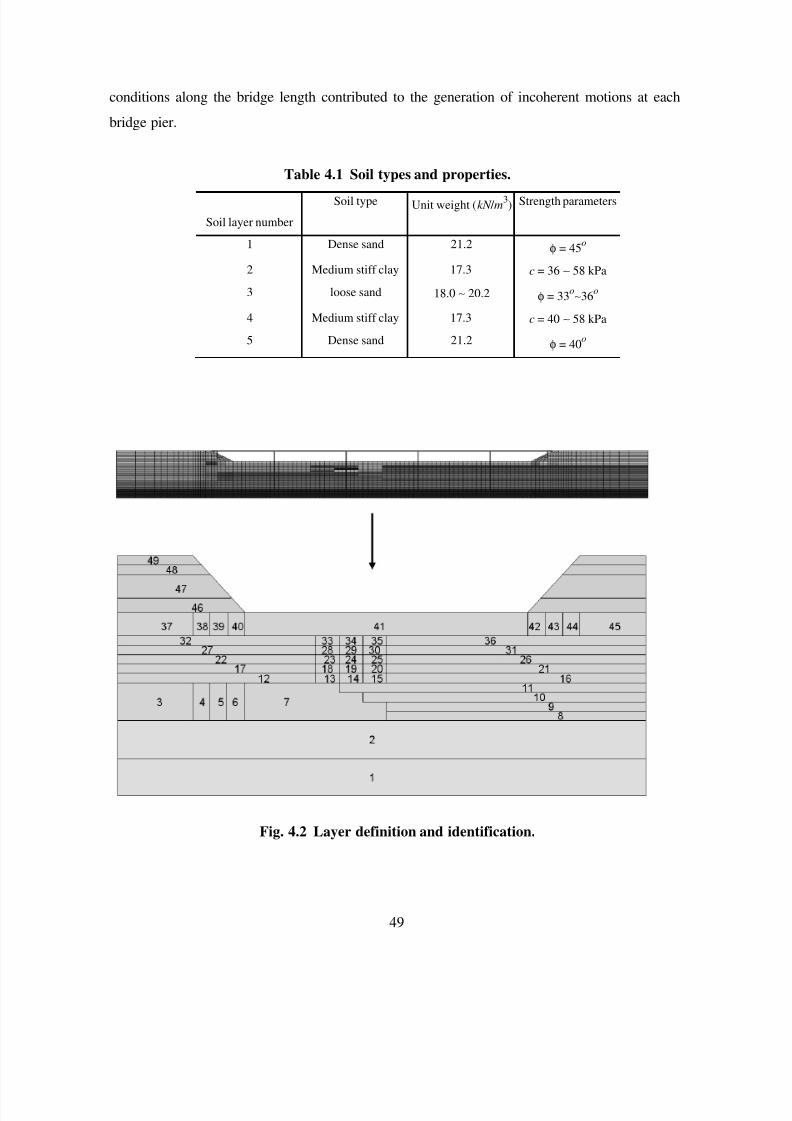
7/21/2019 PEER807 KRAMERArduino Shin
http://slidepdf.com/reader/full/peer807-kramerarduino-shin 63/198
49
conditions along the bridge length contributed to the generation of incoherent motions at each
bridge pier.
Table 4.1 Soil types and properties.
Soil layer number
Soil type Unit weight (kN / m3) Strength parameters
1 Dense sand 21.2 φ = 45o
2 Medium stiff clay 17.3 c = 36 ∼ 58 kPa
3 loose sand 18.0 ∼ 20.2 φ = 33o∼36
o
4 Medium stiff clay 17.3 c = 40 ∼ 58 kPa
5 Dense sand 21.2 φ = 40o
Fig. 4.2 Layer definition and identification.
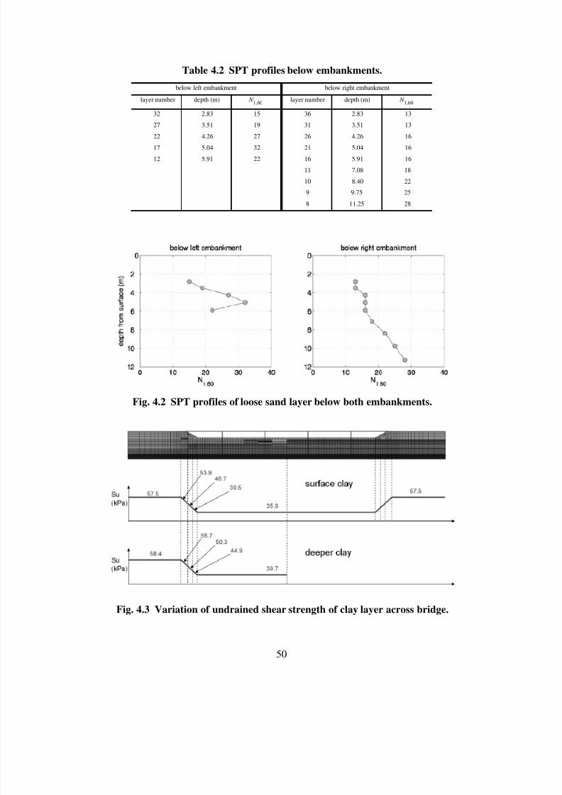
7/21/2019 PEER807 KRAMERArduino Shin
http://slidepdf.com/reader/full/peer807-kramerarduino-shin 64/198
50
Table 4.2 SPT profiles below embankments.
below left embankment below right embankment
layer number depth (m) N 1,60
layer number depth (m) N 1,60
32 2.83 15 36 2.83 13
27 3.51 19 31 3.51 13
22 4.26 27 26 4.26 16
17 5.04 32 21 5.04 16
12 5.91 22 16 5.91 16
11 7.08 18
10 8.40 22
9 9.75 25
8 11.25 28
Fig. 4.2 SPT profiles of loose sand layer below both embankments.
Fig. 4.3 Variation of undrained shear strength of clay layer across bridge.
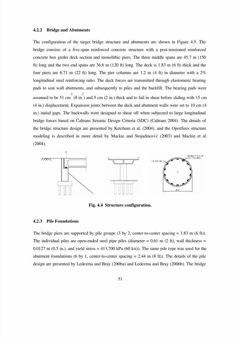
7/21/2019 PEER807 KRAMERArduino Shin
http://slidepdf.com/reader/full/peer807-kramerarduino-shin 65/198
51
4.2.2 Bridge and Abutments
The configuration of the target bridge structure and abutments are shown in Figure 4.5. The
bridge consists of a five-span reinforced concrete structure with a post-tensioned reinforced
concrete box girder deck section and monolithic piers. The three middle spans are 45.7 m (150
ft) long and the two end spans are 36.6 m (120 ft) long. The deck is 1.83 m (6 ft) thick and the
four piers are 6.71 m (22 ft) long. The pier columns are 1.2 m (4 ft) in diameter with a 2%
longitudinal steel reinforcing ratio. The deck forces are transmitted through elastomeric bearing
pads to seat wall abutments, and subsequently to piles and the backfill. The bearing pads were
assumed to be 51 cm2
(8 in2
) and 5 cm (2 in.) thick and to fail in shear before sliding with 15 cm
(4 in.) displacement. Expansion joints between the deck and abutment walls were set to 10 cm (4
in.) initial gaps. The backwalls were designed to shear off when subjected to large longitudinal
bridge forces based on Caltrans Seismic Design Criteria (SDC) (Caltrans 2004). The details of
the bridge structure design are presented by Ketchum et al. (2004), and the OpenSees structure
modeling is described in more detail by Mackie and Stojadinović (2003) and Mackie et al.
(2004).
Fig. 4.4 Structure configuration.
4.2.3 Pile Foundations
The bridge piers are supported by pile groups (3 by 2, center-to-center spacing = 1.83 m (6 ft)).
The individual piles are open-ended steel pipe piles (diameter = 0.61 m (2 ft), wall thickness =
0.0127 m (0.5 in.), and yield stress = 413,700 kPa (60 ksi)). The same pile type was used for the
abutment foundations (6 by 1, center-to-center spacing = 2.44 m (8 ft)). The details of the pile
design are presented by Ledezma and Bray (2006a) and Ledezma and Bray (2006b). The bridge

7/21/2019 PEER807 KRAMERArduino Shin
http://slidepdf.com/reader/full/peer807-kramerarduino-shin 66/198
52
piers and pile groups are labeled from the left abutment to the right as Pier 1, Pier 2, Pier 3, Pier
4, and Pile 1, Pile 2, Pile 3, Pile 4, respectively. The abutment pile groups in the left and right
slopes are labeled as Pile 0 and Pile 5. The abutment piles were assumed to be installed to the
same depth as the other bridge piles.
4.3 SUMMARY
A testbed bridge and soil profile were selected for use in illustrating application of the PEER
PBEE methodology to a realistically complex problem. The bridge structure was designed by a
structural consulting firm with extensive experience in the design of highway bridges for the
California Department of Transportation. The characteristics of the soil profile were selected to
produce liquefaction and lateral spreading beneath the abutments under moderate to strongshaking. The potentially liquefiable soils were thicker under one abutment than the other, and a
layer of clay existed beneath one side of the bridge but not the other. ‘The purpose of the
variable soil conditions was to undue permanent soil deformations in the vicinities of the
abutments under strong shaking so that significant kinematic and inertial interaction was induced
in the bridge and its foundations.
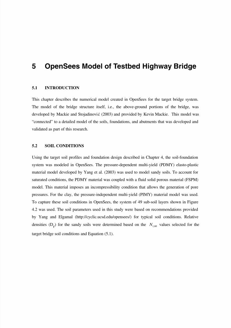
7/21/2019 PEER807 KRAMERArduino Shin
http://slidepdf.com/reader/full/peer807-kramerarduino-shin 67/198
53
5 OpenSees Model of Testbed Highway Bridge
5.1 INTRODUCTION
This chapter describes the numerical model created in OpenSees for the target bridge system.
The model of the bridge structure itself, i.e., the above-ground portions of the bridge, was
developed by Mackie and Stojadinović (2003) and provided by Kevin Mackie. This model was
“connected” to a detailed model of the soils, foundations, and abutments that was developed and
validated as part of this research.
5.2 SOIL CONDITIONS
Using the target soil profiles and foundation design described in Chapter 4, the soil-foundation
system was modeled in OpenSees. The pressure-dependent multi-yield (PDMY) elasto-plastic
material model developed by Yang et al. (2003) was used to model sandy soils. To account for
saturated conditions, the PDMY material was coupled with a fluid solid porous material (FSPM)
model. This material imposes an incompressibility condition that allows the generation of pore
pressures. For the clay, the pressure-independent multi-yield (PIMY) material model was used.
To capture these soil conditions in OpenSees, the system of 49 sub-soil layers shown in Figure
4.2 was used. The soil parameters used in this study were based on recommendations provided
by Yang and Elgamal (http://cyclic.ucsd.edu/opensees/) for typical soil conditions. Relative
densities (Dr) for the sandy soils were determined based on the 60,1 N values selected for the
target bridge soil conditions and Equation (5.1).

7/21/2019 PEER807 KRAMERArduino Shin
http://slidepdf.com/reader/full/peer807-kramerarduino-shin 68/198
54
( )2
60,1 60 r D N = (5.1)
Then, using the recommended values, the 16 material parameters required for the PDMY model
for each sublayer were obtained by interpolation of relative densities. The interpolation was
performed in the 40% to 75% relative density range, where the model parameters show a linear
relationship with relative density. Figure 5.1 shows the interpolated parameter values. The PIMY
material parameters for clay were interpolated in the same way using the selected undrained
shear strength values. The soil parameter values for 49 sublayers of sand and clay are tabulated
with layer number in Tables 5.1 and 5.2. A total of 3874 quadrilateral finite elements and 4050
nodes were used to represent the soil domain.
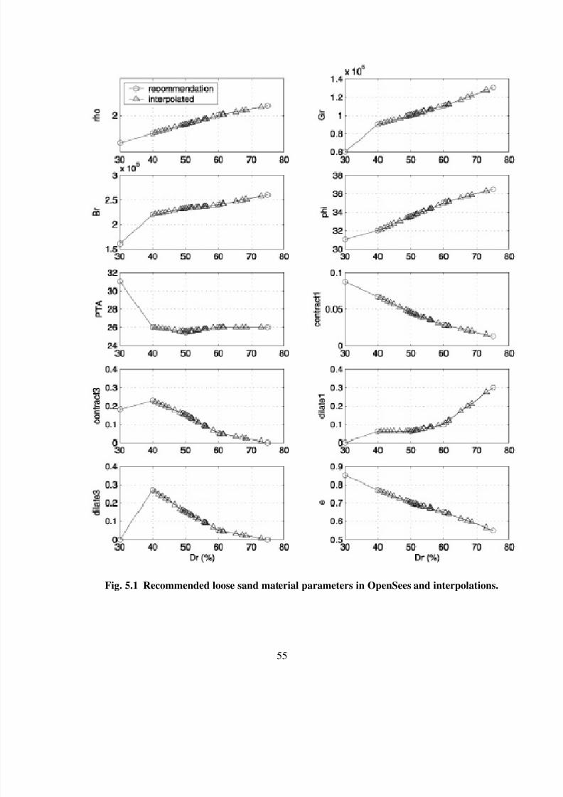
7/21/2019 PEER807 KRAMERArduino Shin
http://slidepdf.com/reader/full/peer807-kramerarduino-shin 69/198
55
Fig. 5.1 Recommended loose sand material parameters in OpenSees and interpolations.
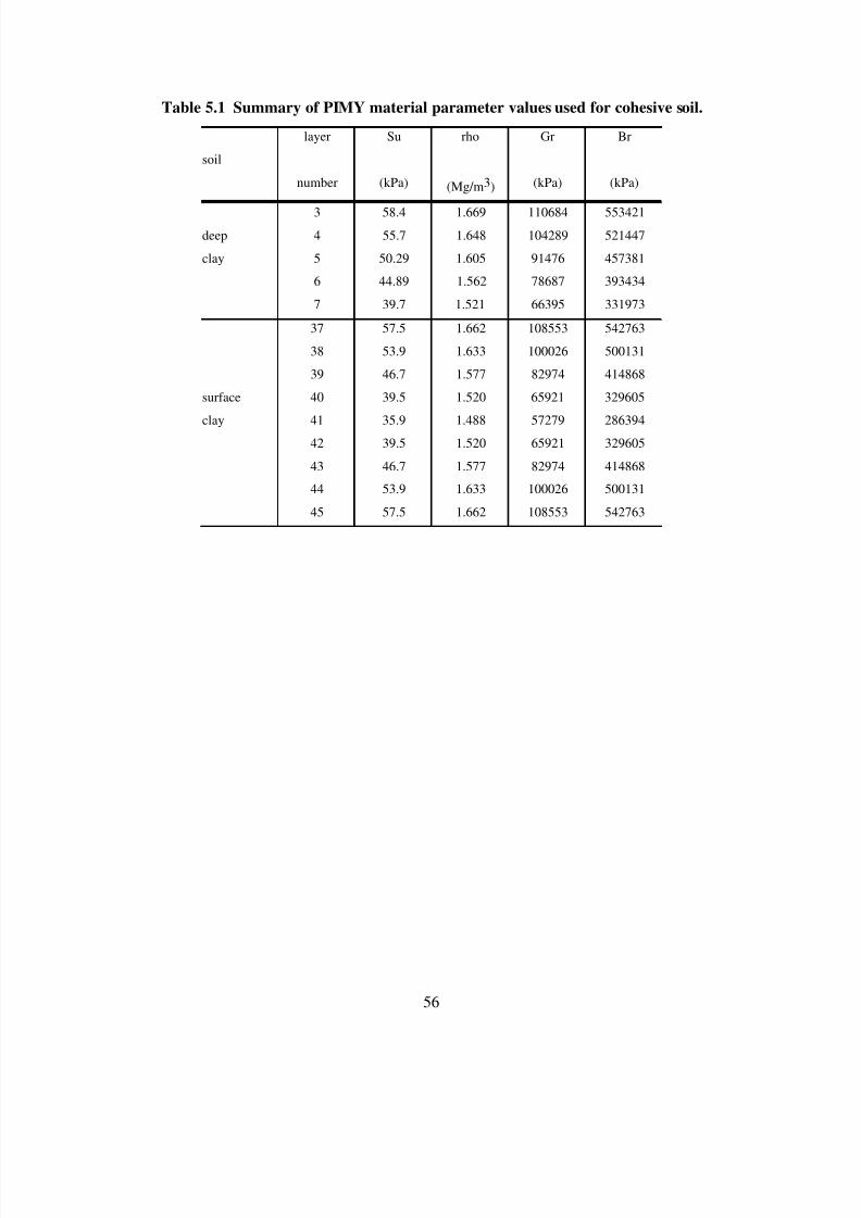
7/21/2019 PEER807 KRAMERArduino Shin
http://slidepdf.com/reader/full/peer807-kramerarduino-shin 70/198
56
Table 5.1 Summary of PIMY material parameter values used for cohesive soil.
soil
layer Su rho Gr Br
number (kPa) (Mg/m3) (kPa) (kPa)
3 58.4 1.669 110684 553421
deep 4 55.7 1.648 104289 521447
clay 5 50.29 1.605 91476 457381
6 44.89 1.562 78687 393434
7 39.7 1.521 66395 331973
37 57.5 1.662 108553 542763
38 53.9 1.633 100026 500131
39 46.7 1.577 82974 414868
surface 40 39.5 1.520 65921 329605
clay 41 35.9 1.488 57279 286394
42 39.5 1.520 65921 329605
43 46.7 1.577 82974 414868
44 53.9 1.633 100026 500131
45 57.5 1.662 108553 542763

7/21/2019 PEER807 KRAMERArduino Shin
http://slidepdf.com/reader/full/peer807-kramerarduino-shin 71/198
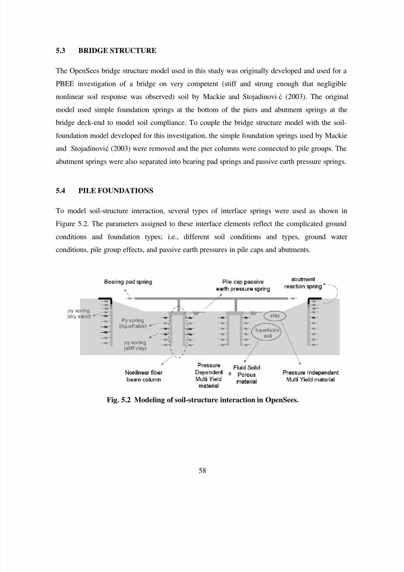
7/21/2019 PEER807 KRAMERArduino Shin
http://slidepdf.com/reader/full/peer807-kramerarduino-shin 72/198
58
5.3 BRIDGE STRUCTURE
The OpenSees bridge structure model used in this study was originally developed and used for a
PBEE investigation of a bridge on very competent (stiff and strong enough that negligible
nonlinear soil response was observed) soil by Mackie and Stojadinović (2003). The original
model used simple foundation springs at the bottom of the piers and abutment springs at the
bridge deck-end to model soil compliance. To couple the bridge structure model with the soil-
foundation model developed for this investigation, the simple foundation springs used by Mackie
and Stojadinović (2003) were removed and the pier columns were connected to pile groups. The
abutment springs were also separated into bearing pad springs and passive earth pressure springs.
5.4 PILE FOUNDATIONS
To model soil-structure interaction, several types of interface springs were used as shown in
Figure 5.2. The parameters assigned to these interface elements reflect the complicated ground
conditions and foundation types; i.e., different soil conditions and types, ground water
conditions, pile group effects, and passive earth pressures in pile caps and abutments.
Fig. 5.2 Modeling of soil-structure interaction in OpenSees.
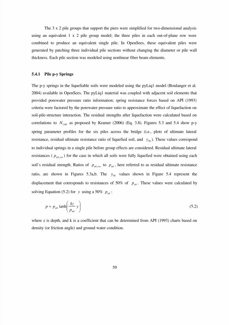
7/21/2019 PEER807 KRAMERArduino Shin
http://slidepdf.com/reader/full/peer807-kramerarduino-shin 73/198
59
The 3 x 2 pile groups that support the piers were simplified for two-dimensional analysis
using an equivalent 1 x 2 pile group model; the three piles in each out-of-plane row were
combined to produce an equivalent single pile. In OpenSees, these equivalent piles were
generated by patching three individual pile sections without changing the diameter or pile wall
thickness. Each pile section was modeled using nonlinear fiber beam elements.
5.4.1 Pile p-y Springs
The p-y springs in the liquefiable soils were modeled using the pyLiq1 model (Boulanger et al.
2004) available in OpenSees. The pyLiq1 material was coupled with adjacent soil elements that
provided porewater pressure ratio information; spring resistance forces based on API (1993)
criteria were factored by the porewater pressure ratio to approximate the effect of liquefaction onsoil-pile-structure interaction. The residual strengths after liquefaction were calculated based on
correlations to 60,1 N as proposed by Kramer (2006) (Eq. 3.8). Figures 5.3 and 5.4 show p-y
spring parameter profiles for the six piles across the bridge (i.e., plots of ultimate lateral
resistance, residual ultimate resistance ratio of liquefied soil, and 50 y ). These values correspond
to individual springs in a single pile before group effects are considered. Residual ultimate lateral
resistances ( result p , ) for the case in which all soils were fully liquefied were obtained using each
soil’s residual strength. Ratios of result p , to ult p , here referred to as residual ultimate resistance
ratio, are shown in Figures 5.3a,b. The 50 y values shown in Figure 5.4 represent the
displacement that corresponds to resistances of 50% of ult p . These values were calculated by
solving Equation (5.2) for y using a 50% ult p :
= y
p
kz p p
ult
ult tanh (5.2)
where z is depth, and k is a coefficient that can be determined from API (1993) charts based on
density (or friction angle) and ground water condition.
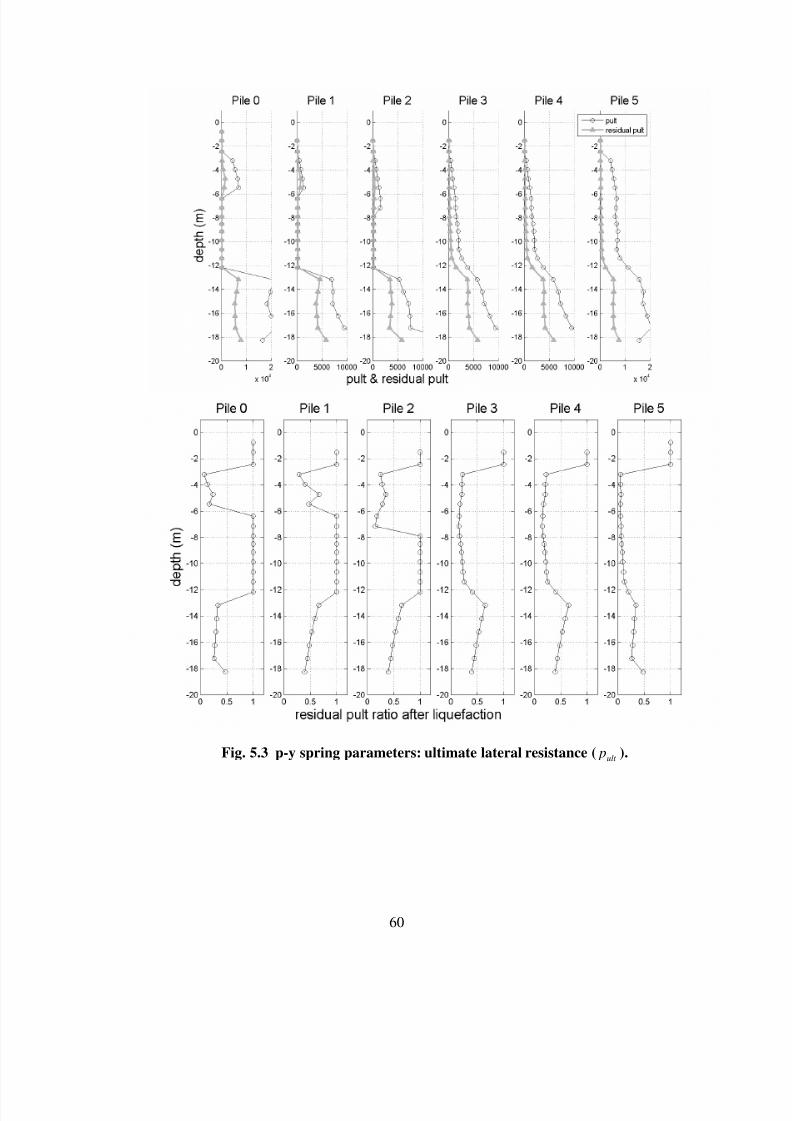
7/21/2019 PEER807 KRAMERArduino Shin
http://slidepdf.com/reader/full/peer807-kramerarduino-shin 74/198
60
Fig. 5.3 p-y spring parameters: ultimate lateral resistance ( ult p ).
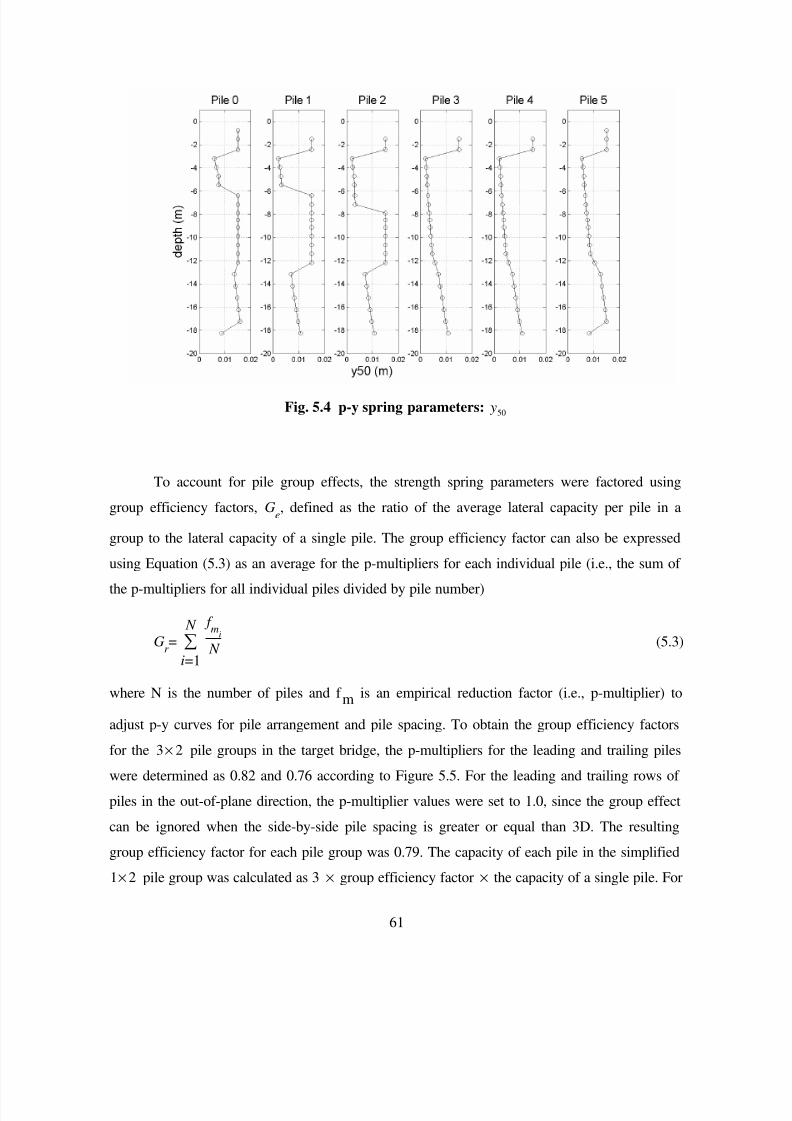
7/21/2019 PEER807 KRAMERArduino Shin
http://slidepdf.com/reader/full/peer807-kramerarduino-shin 75/198
61
Fig. 5.4 p-y spring parameters: 50 y
To account for pile group effects, the strength spring parameters were factored using
group efficiency factors, Ge, defined as the ratio of the average lateral capacity per pile in a
group to the lateral capacity of a single pile. The group efficiency factor can also be expressed
using Equation (5.3) as an average for the p-multipliers for each individual pile (i.e., the sum of
the p-multipliers for all individual piles divided by pile number)
Gr = ∑
i=1
N
f m
i
N (5.3)
where N is the number of piles and f m is an empirical reduction factor (i.e., p-multiplier) to
adjust p-y curves for pile arrangement and pile spacing. To obtain the group efficiency factors
for the 23× pile groups in the target bridge, the p-multipliers for the leading and trailing piles
were determined as 0.82 and 0.76 according to Figure 5.5. For the leading and trailing rows of
piles in the out-of-plane direction, the p-multiplier values were set to 1.0, since the group effect
can be ignored when the side-by-side pile spacing is greater or equal than 3D. The resulting
group efficiency factor for each pile group was 0.79. The capacity of each pile in the simplified
21× pile group was calculated as 3 × group efficiency factor × the capacity of a single pile. For
7/21/2019 PEER807 KRAMERArduino Shin
http://slidepdf.com/reader/full/peer807-kramerarduino-shin 76/198
62
the 61× pile groups under the abutments, no group effects were considered, since they have a
single row of piles and the side-by-side pile spacing (4D) is greater than 3D. The skin resistance
and pile tip resistance was modeled using t-z and q-z springs. These springs were assumed to
have no group effects.
5.4.2 Pile Cap Passive Earth Pressure Springs
To capture the response of the pile caps, three passive earth pressure springs were used at the
top, middle, and bottom of the cap. The clay passive earth pressure envelope of the pile cap was
determined using the 0=φ sliding wedge method (Eq. 3.13) suggested by Mokwa (1999). It was
assumed that the bridge longitudinal and transverse pile cap lengths were 3.6 m (12 ft) and 5.4 m
(18 ft), respectively, and that the pile cap height was 1.5 m (5 ft). An adhesion factor ( α ) of 0.75
was used in the method for the medium stiff clay.
5.5 ABUTMENT INTERFACE SPRINGS
The height of the backwall (break-off wall) was 1.8 m (6ft) and its width was 13.7 m (45 ft). The
interaction between the bridge deck and abutment was decomposed into two interaction
components. A schematic of the bridge deck-abutment interaction and its modeling are shown in
Figures 3.18 and 5.15. The first component combined the bearing pad resistance and backwall
resistance in a single spring model. This spring force was transferred to the stem wall and
abutment pile foundation. The stem wall was connected to the soil without interface assuming its
relative displacement was small. The second component included the expansion joint gap and
backwall lateral soil resistance. In this case the force-displacement envelope was obtained by
combining a gap spring and a soil spring whose parameters were obtained based on Caltrans’s
Seismic Design Criteria (Caltrans 2004). For the selected abutments, the initial stiffness and
ultimate resistance used were 164,300 kN/m/m (20 kips/in/ft) and 6,258kN (1290 kips),
respectively.
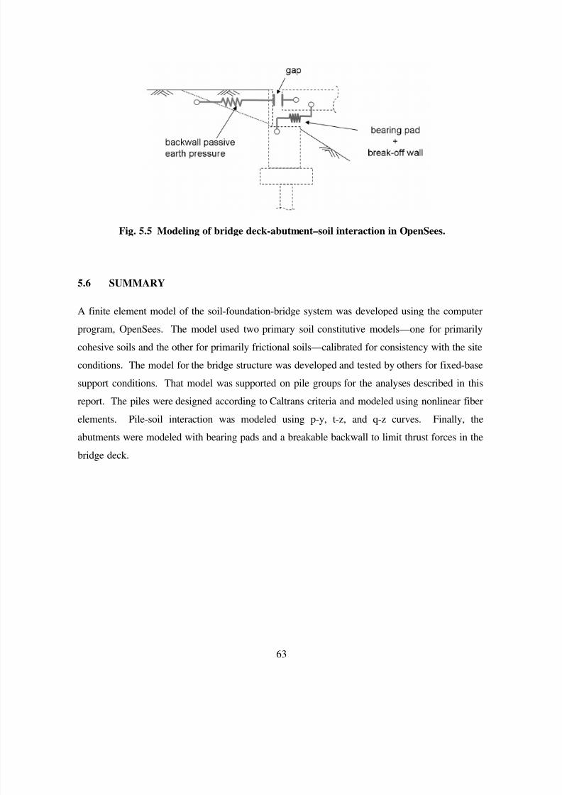
7/21/2019 PEER807 KRAMERArduino Shin
http://slidepdf.com/reader/full/peer807-kramerarduino-shin 77/198
63
Fig. 5.5 Modeling of bridge deck-abutment–soil interaction in OpenSees.
5.6 SUMMARY
A finite element model of the soil-foundation-bridge system was developed using the computer
program, OpenSees. The model used two primary soil constitutive models—one for primarily
cohesive soils and the other for primarily frictional soils—calibrated for consistency with the site
conditions. The model for the bridge structure was developed and tested by others for fixed-base
support conditions. That model was supported on pile groups for the analyses described in this
report. The piles were designed according to Caltrans criteria and modeled using nonlinear fiber
elements. Pile-soil interaction was modeled using p-y, t-z, and q-z curves. Finally, the
abutments were modeled with bearing pads and a breakable backwall to limit thrust forces in the
bridge deck.
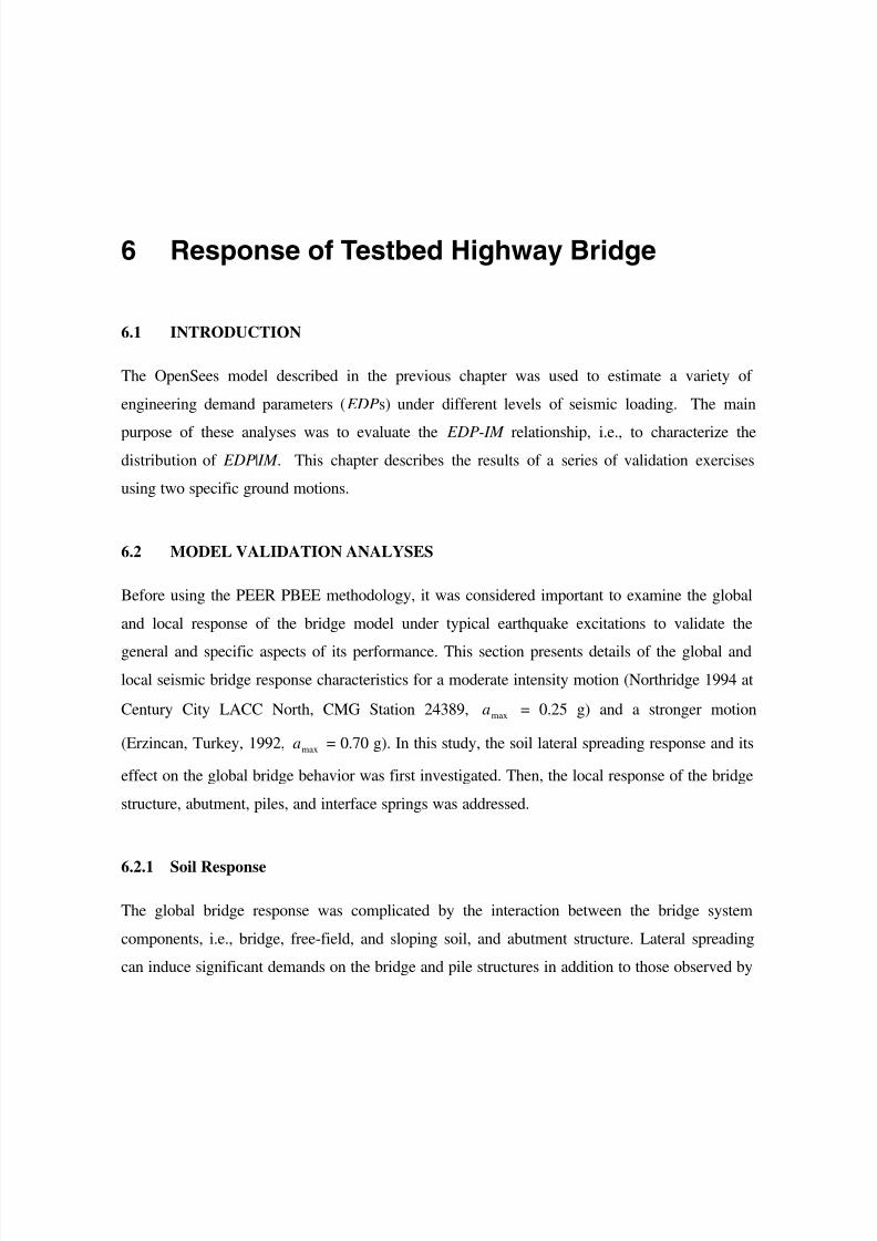
7/21/2019 PEER807 KRAMERArduino Shin
http://slidepdf.com/reader/full/peer807-kramerarduino-shin 78/198
65
6 Response of Testbed Highway Bridge
6.1 INTRODUCTION
The OpenSees model described in the previous chapter was used to estimate a variety of
engineering demand parameters ( EDPs) under different levels of seismic loading. The main
purpose of these analyses was to evaluate the EDP- IM relationship, i.e., to characterize the
distribution of EDP| IM . This chapter describes the results of a series of validation exercises
using two specific ground motions.
6.2 MODEL VALIDATION ANALYSES
Before using the PEER PBEE methodology, it was considered important to examine the global
and local response of the bridge model under typical earthquake excitations to validate the
general and specific aspects of its performance. This section presents details of the global and
local seismic bridge response characteristics for a moderate intensity motion (Northridge 1994 at
Century City LACC North, CMG Station 24389, maxa = 0.25 g) and a stronger motion
(Erzincan, Turkey, 1992, maxa = 0.70 g). In this study, the soil lateral spreading response and its
effect on the global bridge behavior was first investigated. Then, the local response of the bridge
structure, abutment, piles, and interface springs was addressed.
6.2.1 Soil Response
The global bridge response was complicated by the interaction between the bridge system
components, i.e., bridge, free-field, and sloping soil, and abutment structure. Lateral spreading
can induce significant demands on the bridge and pile structures in addition to those observed by
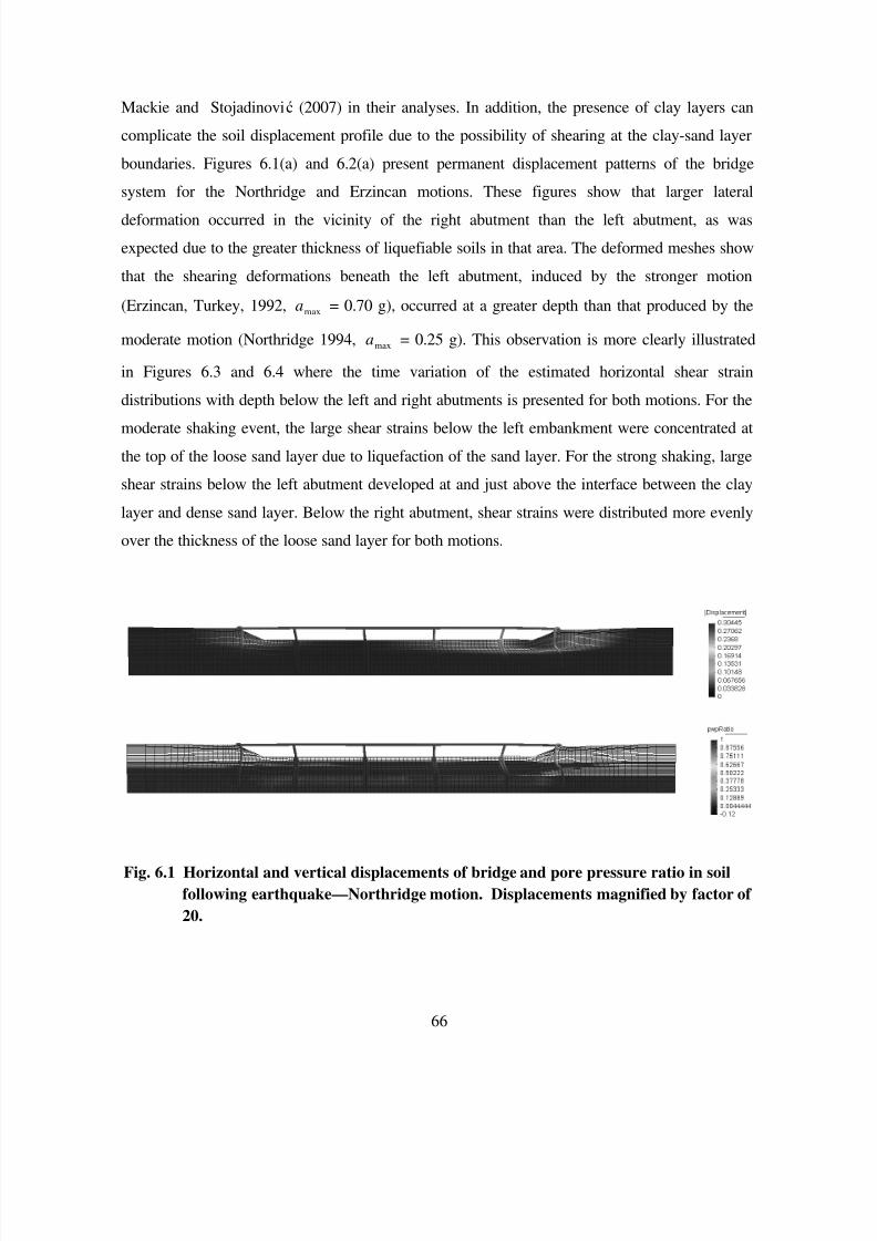
7/21/2019 PEER807 KRAMERArduino Shin
http://slidepdf.com/reader/full/peer807-kramerarduino-shin 79/198
66
Mackie and Stojadinović (2007) in their analyses. In addition, the presence of clay layers can
complicate the soil displacement profile due to the possibility of shearing at the clay-sand layer
boundaries. Figures 6.1(a) and 6.2(a) present permanent displacement patterns of the bridge
system for the Northridge and Erzincan motions. These figures show that larger lateral
deformation occurred in the vicinity of the right abutment than the left abutment, as was
expected due to the greater thickness of liquefiable soils in that area. The deformed meshes show
that the shearing deformations beneath the left abutment, induced by the stronger motion
(Erzincan, Turkey, 1992, maxa = 0.70 g), occurred at a greater depth than that produced by the
moderate motion (Northridge 1994, maxa = 0.25 g). This observation is more clearly illustrated
in Figures 6.3 and 6.4 where the time variation of the estimated horizontal shear strain
distributions with depth below the left and right abutments is presented for both motions. For the
moderate shaking event, the large shear strains below the left embankment were concentrated at
the top of the loose sand layer due to liquefaction of the sand layer. For the strong shaking, large
shear strains below the left abutment developed at and just above the interface between the clay
layer and dense sand layer. Below the right abutment, shear strains were distributed more evenly
over the thickness of the loose sand layer for both motions.
Fig. 6.1 Horizontal and vertical displacements of bridge and pore pressure ratio in soil
following earthquake—Northridge motion. Displacements magnified by factor of
20.
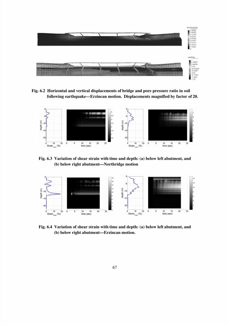
7/21/2019 PEER807 KRAMERArduino Shin
http://slidepdf.com/reader/full/peer807-kramerarduino-shin 80/198
67
Fig. 6.2 Horizontal and vertical displacements of bridge and pore pressure ratio in soil
following earthquake—Erzincan motion. Displacements magnified by factor of 20.
Fig. 6.3 Variation of shear strain with time and depth: (a) below left abutment, and
(b) below right abutment—Northridge motion
Fig. 6.4 Variation of shear strain with time and depth: (a) below left abutment, and
(b) below right abutment—Erzincan motion.

7/21/2019 PEER807 KRAMERArduino Shin
http://slidepdf.com/reader/full/peer807-kramerarduino-shin 81/198
68
To show the degree of liquefaction in the soil beneath the right abutment, pore pressure
ratios measured at several soil locations are shown in Figure 6.5(a). The pore pressure ratio time
histories in the loose sand below the right abutment are shown in Figure 6.5(b) for the moderate
shaking level. The figure shows that the upper layer of the loose sand was fully liquefied across
the right side of the bridge. However, the bottom layer of the loose sand below the embankment
had pore pressure ratios less than 1.0; the soil at this location was slightly denser and had higher
initial effective stress than the soils that were not beneath the embankment. Figure 6.6 shows the
time variation of pore pressure ratio with depth below the right abutment for the Northridge
motion illustrating different degrees of pore pressure generation with time.
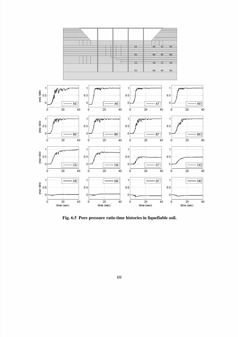
7/21/2019 PEER807 KRAMERArduino Shin
http://slidepdf.com/reader/full/peer807-kramerarduino-shin 82/198
69
Fig. 6.5 Pore pressure ratio time histories in liquefiable soil.
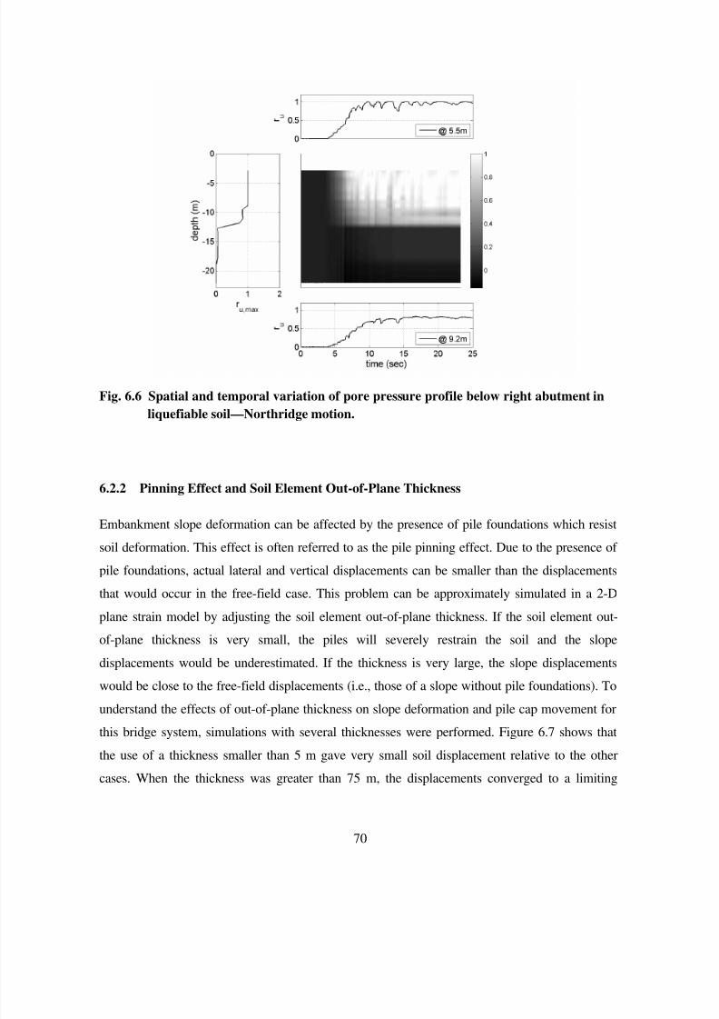
7/21/2019 PEER807 KRAMERArduino Shin
http://slidepdf.com/reader/full/peer807-kramerarduino-shin 83/198
70
Fig. 6.6 Spatial and temporal variation of pore pressure profile below right abutment in
liquefiable soil—Northridge motion.
6.2.2 Pinning Effect and Soil Element Out-of-Plane Thickness
Embankment slope deformation can be affected by the presence of pile foundations which resist
soil deformation. This effect is often referred to as the pile pinning effect. Due to the presence of
pile foundations, actual lateral and vertical displacements can be smaller than the displacements
that would occur in the free-field case. This problem can be approximately simulated in a 2-D
plane strain model by adjusting the soil element out-of-plane thickness. If the soil element out-
of-plane thickness is very small, the piles will severely restrain the soil and the slope
displacements would be underestimated. If the thickness is very large, the slope displacements
would be close to the free-field displacements (i.e., those of a slope without pile foundations). To
understand the effects of out-of-plane thickness on slope deformation and pile cap movement for
this bridge system, simulations with several thicknesses were performed. Figure 6.7 shows that
the use of a thickness smaller than 5 m gave very small soil displacement relative to the other
cases. When the thickness was greater than 75 m, the displacements converged to a limiting
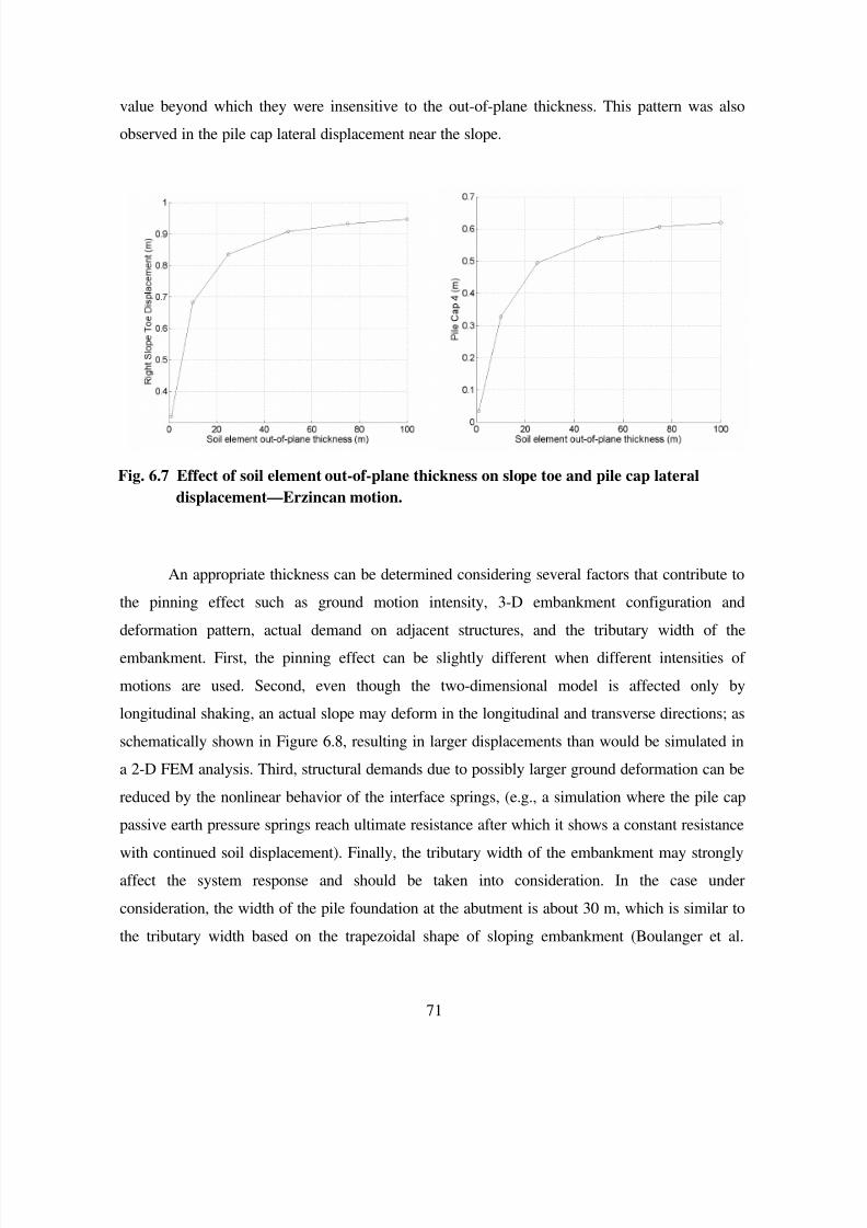
7/21/2019 PEER807 KRAMERArduino Shin
http://slidepdf.com/reader/full/peer807-kramerarduino-shin 84/198
71
value beyond which they were insensitive to the out-of-plane thickness. This pattern was also
observed in the pile cap lateral displacement near the slope.
Fig. 6.7 Effect of soil element out-of-plane thickness on slope toe and pile cap lateral
displacement—Erzincan motion.
An appropriate thickness can be determined considering several factors that contribute to
the pinning effect such as ground motion intensity, 3-D embankment configuration and
deformation pattern, actual demand on adjacent structures, and the tributary width of the
embankment. First, the pinning effect can be slightly different when different intensities of
motions are used. Second, even though the two-dimensional model is affected only by
longitudinal shaking, an actual slope may deform in the longitudinal and transverse directions; as
schematically shown in Figure 6.8, resulting in larger displacements than would be simulated in
a 2-D FEM analysis. Third, structural demands due to possibly larger ground deformation can be
reduced by the nonlinear behavior of the interface springs, (e.g., a simulation where the pile cap
passive earth pressure springs reach ultimate resistance after which it shows a constant resistance
with continued soil displacement). Finally, the tributary width of the embankment may strongly
affect the system response and should be taken into consideration. In the case under
consideration, the width of the pile foundation at the abutment is about 30 m, which is similar to
the tributary width based on the trapezoidal shape of sloping embankment (Boulanger et al.

7/21/2019 PEER807 KRAMERArduino Shin
http://slidepdf.com/reader/full/peer807-kramerarduino-shin 85/198
72
2005). For these reasons, a 50 m soil element out-of-plane thickness was chosen for the analysis.
For improved estimation of out-of-plane thickness effects, 3-D model studies are required.
This is certainly a limitation of two-dimensional analysis (performed in this study).
However, two-dimensional analysis brings the possibility to evaluate the response of the
complete structure in a logical way, while keeping the computational time at reasonable levels.
Fig. 6.8 Schematic drawing of 3-D embankment deformation.
6.2.3 Global Behavior of Bridge System
The numerical simulations showed that the expansion joints between the bridge deck and
abutment backwalls close when lateral spreading occurred. Since the amount of lateral spreading
beneath the right abutment was considerably larger than that beneath the left abutment, the entire
bridge deck tended to be pushed to the left. At the same time, lateral spreading also pushed the
pile cap of Pier 4 to the left resulting in relatively small drift in that column. On the other hand,
Pier 1 was subjected to large column drift because the bridge deck moved the upper end of the
column to the left while lateral spreading moved the pile cap at the base of the column to the
right. This global bridge behavior, which would likely not be anticipated by typical analyses that
model only individual parts of the bridge, greatly affected the demands on many local
components of the bridge. The details of the local response of bridge piers, abutments, and piles
are discussed in the following sections.

7/21/2019 PEER807 KRAMERArduino Shin
http://slidepdf.com/reader/full/peer807-kramerarduino-shin 86/198
73
6.2.4 Bridge Pier Response
The bridge pier response was investigated using the displacements of the bridge deck and pile
cap. Figure 6.9(b) shows drift ratios associated with the difference in displacement between the
tops and bottoms of piers. The bottoms of the four piers (pile caps) moved toward the center of
the bridge by amounts that varied due to different levels of lateral spreading. As shown in Figure
6.9(a), Pier 1 base residual lateral displacement was about 20 cm after shaking and Pier 4 base
residual lateral displacement was about 60 cm. In the meantime, the tops of all piers moved to
the left as the larger lateral spreading beneath the right abutment pushed the entire bridge deck to
the left. This bridge deck movement increased Pier 1 drift and decreased Pier 4 drift. Due to this
global response, similar drift ratios were observed in Pier 1 and Pier 4 for this particular motion
even though the base residual lateral displacement of Pier 4 was much greater than that of Pier 1.These analyses demonstrated that lateral spreading in an abutment slope can affect the column
drift in the other side of bridge.
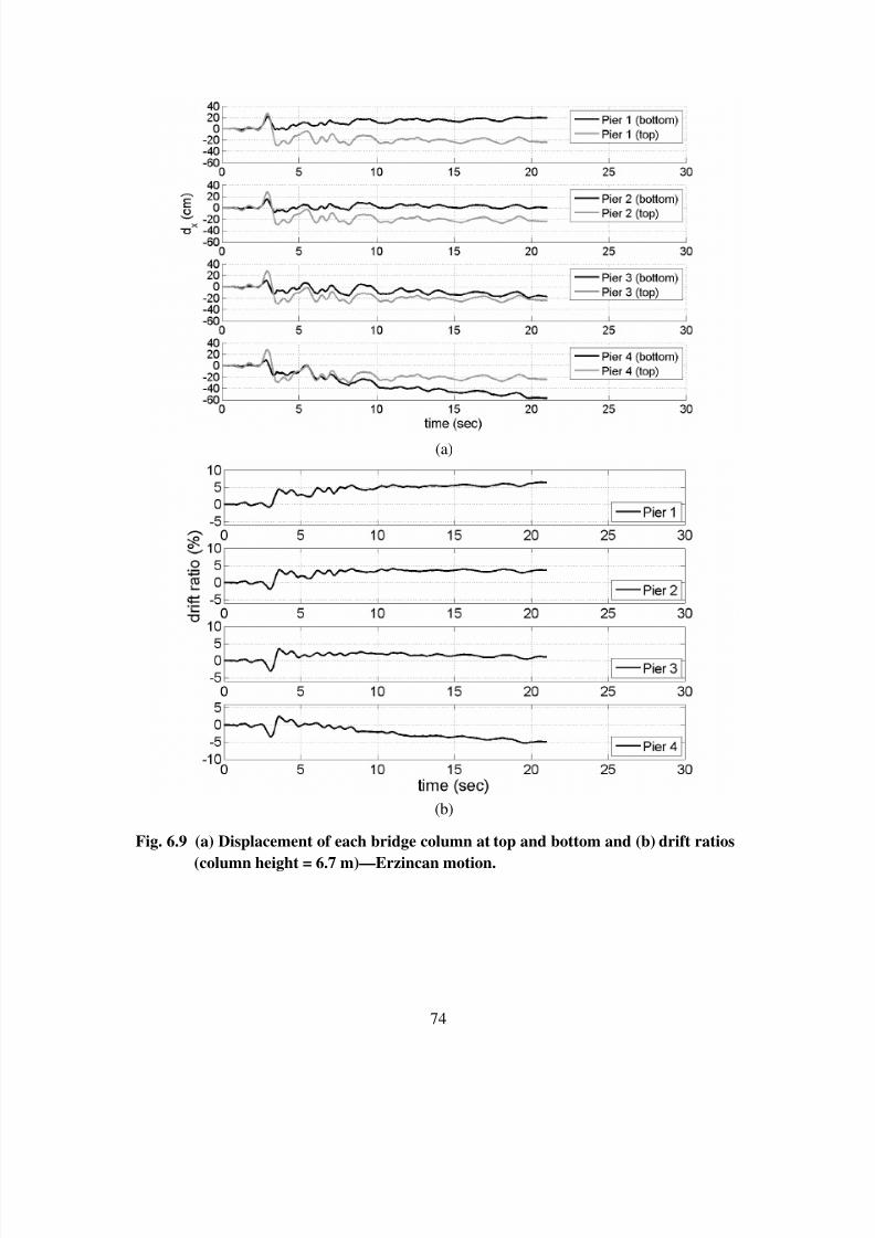
7/21/2019 PEER807 KRAMERArduino Shin
http://slidepdf.com/reader/full/peer807-kramerarduino-shin 87/198
74
(a)
(b)
Fig. 6.9 (a) Displacement of each bridge column at top and bottom and (b) drift ratios
(column height = 6.7 m)—Erzincan motion.
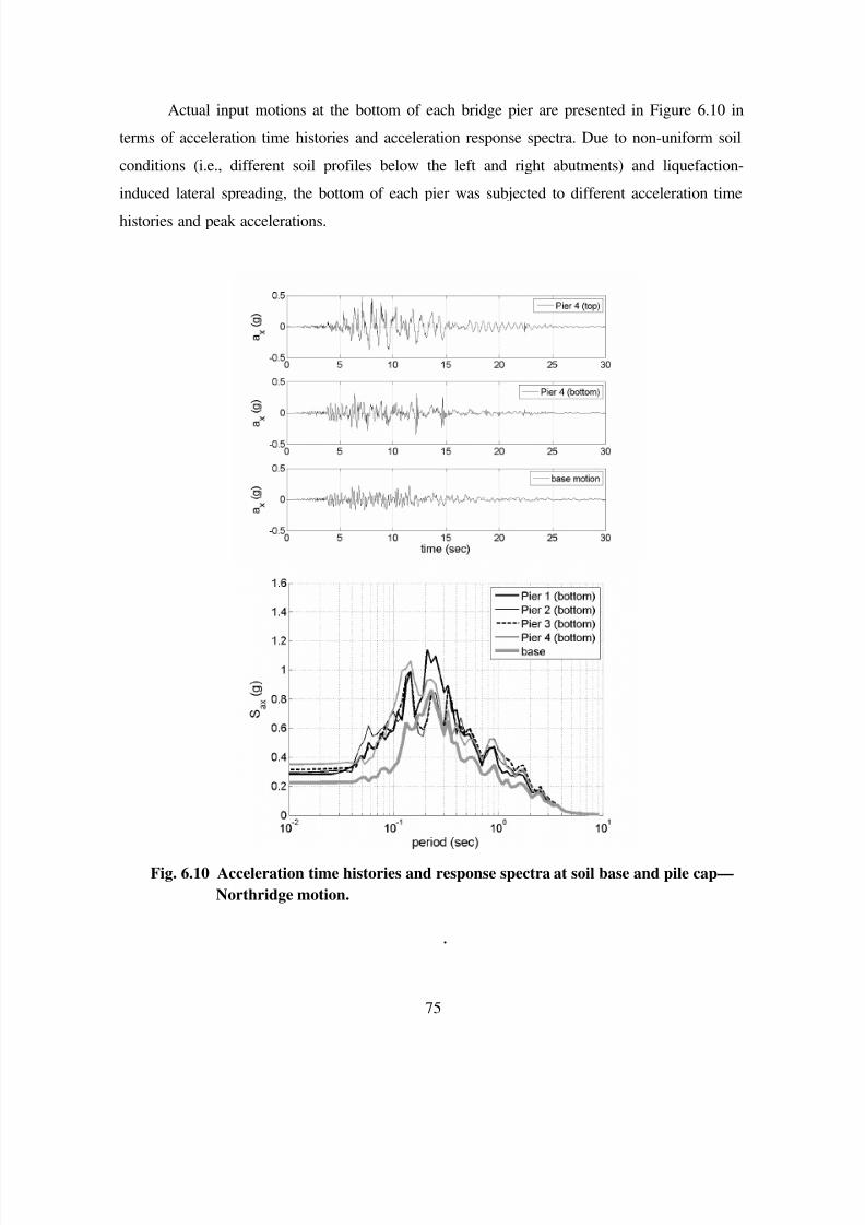
7/21/2019 PEER807 KRAMERArduino Shin
http://slidepdf.com/reader/full/peer807-kramerarduino-shin 88/198
75
Actual input motions at the bottom of each bridge pier are presented in Figure 6.10 in
terms of acceleration time histories and acceleration response spectra. Due to non-uniform soil
conditions (i.e., different soil profiles below the left and right abutments) and liquefaction-
induced lateral spreading, the bottom of each pier was subjected to different acceleration time
histories and peak accelerations.
Fig. 6.10 Acceleration time histories and response spectra at soil base and pile cap—
Northridge motion.
.
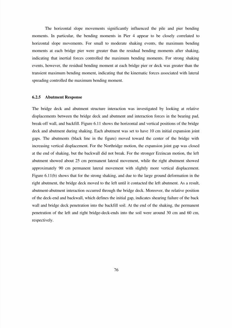
7/21/2019 PEER807 KRAMERArduino Shin
http://slidepdf.com/reader/full/peer807-kramerarduino-shin 89/198
76
The horizontal slope movements significantly influenced the pile and pier bending
moments. In particular, the bending moments in Pier 4 appear to be closely correlated to
horizontal slope movements. For small to moderate shaking events, the maximum bending
moments at each bridge pier were greater than the residual bending moments after shaking,
indicating that inertial forces controlled the maximum bending moments. For strong shaking
events, however, the residual bending moment at each bridge pier or deck was greater than the
transient maximum bending moment, indicating that the kinematic forces associated with lateral
spreading controlled the maximum bending moment.
6.2.5 Abutment Response
The bridge deck and abutment structure interaction was investigated by looking at relativedisplacements between the bridge deck and abutment and interaction forces in the bearing pad,
break-off wall, and backfill. Figure 6.11 shows the horizontal and vertical positions of the bridge
deck and abutment during shaking. Each abutment was set to have 10 cm initial expansion joint
gaps. The abutments (black line in the figure) moved toward the center of the bridge with
increasing vertical displacement. For the Northridge motion, the expansion joint gap was closed
at the end of shaking, but the backwall did not break. For the stronger Erzincan motion, the left
abutment showed about 25 cm permanent lateral movement, while the right abutment showed
approximately 90 cm permanent lateral movement with slightly more vertical displacement.
Figure 6.11(b) shows that for the strong shaking, and due to the large ground deformation in the
right abutment, the bridge deck moved to the left until it contacted the left abutment. As a result,
abutment-abutment interaction occurred through the bridge deck. Moreover, the relative position
of the deck-end and backwall, which defines the initial gap, indicates shearing failure of the back
wall and bridge deck penetration into the backfill soil. At the end of the shaking, the permanent
penetration of the left and right bridge-deck-ends into the soil were around 30 cm and 60 cm,
respectively.
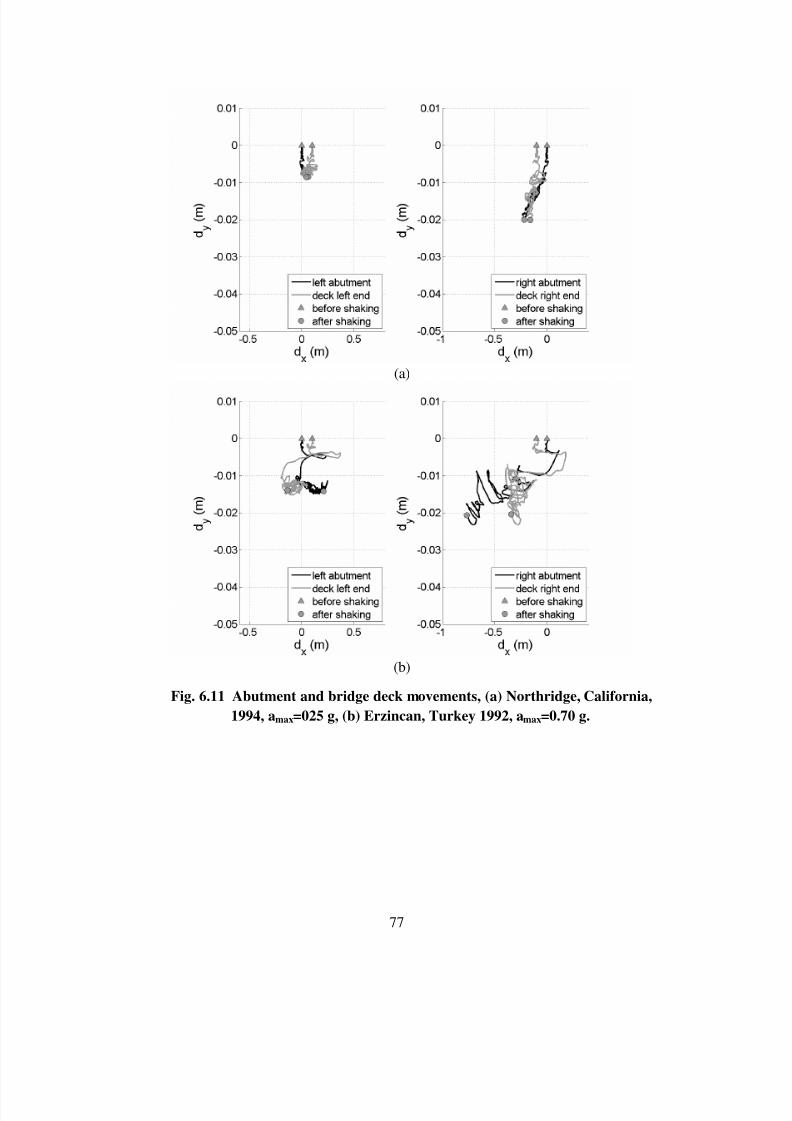
7/21/2019 PEER807 KRAMERArduino Shin
http://slidepdf.com/reader/full/peer807-kramerarduino-shin 90/198
77
(a)
(b)
Fig. 6.11 Abutment and bridge deck movements, (a) Northridge, California,
1994, amax=025 g, (b) Erzincan, Turkey 1992, amax=0.70 g.

7/21/2019 PEER807 KRAMERArduino Shin
http://slidepdf.com/reader/full/peer807-kramerarduino-shin 91/198
78
The bridge deck and abutment interaction is illustrated in Figure 6.12 in terms of spring
force-displacements for a strong shaking event. Figures 6.12(a) and (b) show lateral resistance in
the bearing pad and backwall. After 10 cm of displacement, where bearing pad resistance
develops, large lateral resistance was mobilized in the break-off wall. This wall resistance
disappeared after the wall ultimate resistance was reached. This interaction force was then
transferred to the stem wall of the abutment. Figures 6.12(c) and (d) show that the passive earth
pressure resistance in the backfill soil mobilized after reaching the maximum capacity of the
break-off wall. Figures 6.12(e) and (f) show the total lateral resistance transmitted from the
abutment system to the bridge deck.
7/21/2019 PEER807 KRAMERArduino Shin
http://slidepdf.com/reader/full/peer807-kramerarduino-shin 92/198
79
Fig. 6.12 Bridge deck and abutment interaction force-displacement—Erzincan motion..
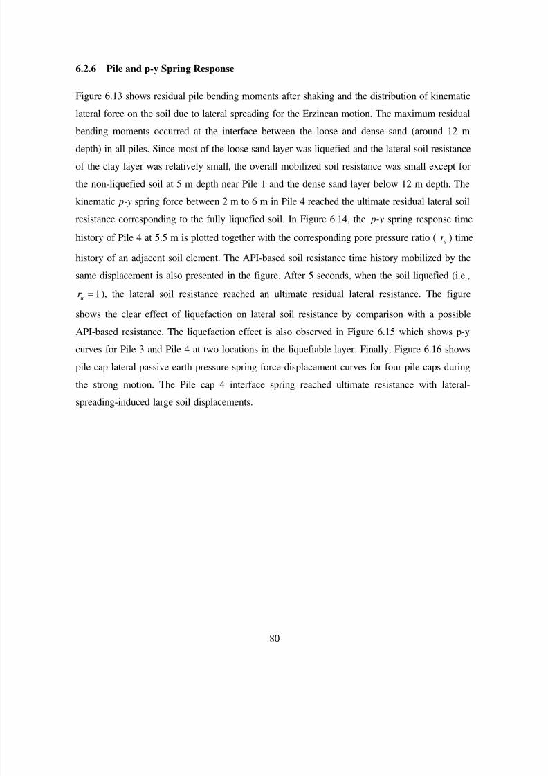
7/21/2019 PEER807 KRAMERArduino Shin
http://slidepdf.com/reader/full/peer807-kramerarduino-shin 93/198
80
6.2.6 Pile and p-y Spring Response
Figure 6.13 shows residual pile bending moments after shaking and the distribution of kinematic
lateral force on the soil due to lateral spreading for the Erzincan motion. The maximum residual
bending moments occurred at the interface between the loose and dense sand (around 12 m
depth) in all piles. Since most of the loose sand layer was liquefied and the lateral soil resistance
of the clay layer was relatively small, the overall mobilized soil resistance was small except for
the non-liquefied soil at 5 m depth near Pile 1 and the dense sand layer below 12 m depth. The
kinematic p-y spring force between 2 m to 6 m in Pile 4 reached the ultimate residual lateral soil
resistance corresponding to the fully liquefied soil. In Figure 6.14, the p-y spring response time
history of Pile 4 at 5.5 m is plotted together with the corresponding pore pressure ratio ( ur ) time
history of an adjacent soil element. The API-based soil resistance time history mobilized by the
same displacement is also presented in the figure. After 5 seconds, when the soil liquefied (i.e.,
1=ur ), the lateral soil resistance reached an ultimate residual lateral resistance. The figure
shows the clear effect of liquefaction on lateral soil resistance by comparison with a possible
API-based resistance. The liquefaction effect is also observed in Figure 6.15 which shows p-y
curves for Pile 3 and Pile 4 at two locations in the liquefiable layer. Finally, Figure 6.16 shows
pile cap lateral passive earth pressure spring force-displacement curves for four pile caps during
the strong motion. The Pile cap 4 interface spring reached ultimate resistance with lateral-spreading-induced large soil displacements.
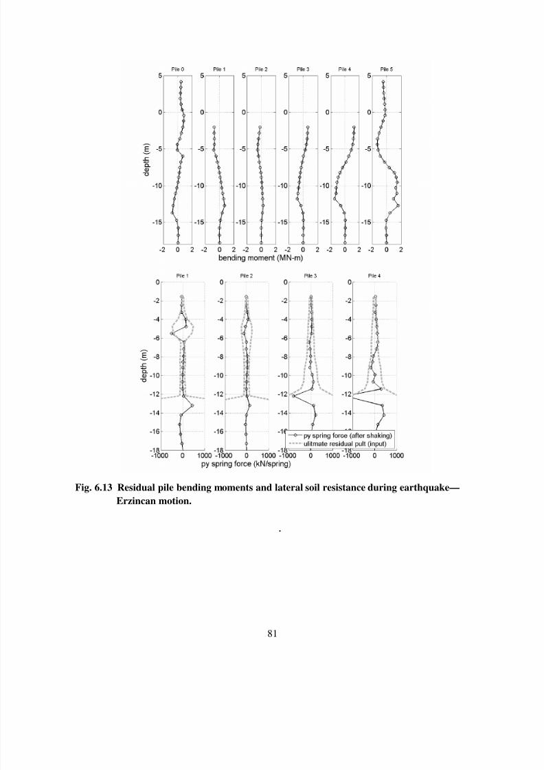
7/21/2019 PEER807 KRAMERArduino Shin
http://slidepdf.com/reader/full/peer807-kramerarduino-shin 94/198
81
Fig. 6.13 Residual pile bending moments and lateral soil resistance during earthquake—
Erzincan motion.
.
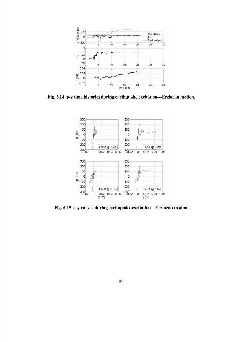
7/21/2019 PEER807 KRAMERArduino Shin
http://slidepdf.com/reader/full/peer807-kramerarduino-shin 95/198
82
Fig. 6.14 p-y time histories during earthquake excitation—Erzincan motion.
Fig. 6.15 p-y curves during earthquake excitation—Erzincan motion.
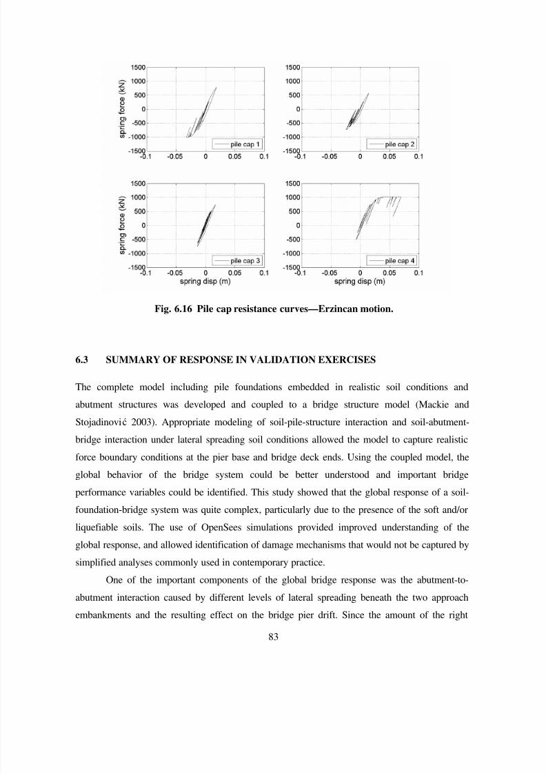
7/21/2019 PEER807 KRAMERArduino Shin
http://slidepdf.com/reader/full/peer807-kramerarduino-shin 96/198
83
Fig. 6.16 Pile cap resistance curves—Erzincan motion.
6.3 SUMMARY OF RESPONSE IN VALIDATION EXERCISES
The complete model including pile foundations embedded in realistic soil conditions and
abutment structures was developed and coupled to a bridge structure model (Mackie and
Stojadinović 2003). Appropriate modeling of soil-pile-structure interaction and soil-abutment-
bridge interaction under lateral spreading soil conditions allowed the model to capture realistic
force boundary conditions at the pier base and bridge deck ends. Using the coupled model, the
global behavior of the bridge system could be better understood and important bridge
performance variables could be identified. This study showed that the global response of a soil-
foundation-bridge system was quite complex, particularly due to the presence of the soft and/or
liquefiable soils. The use of OpenSees simulations provided improved understanding of the
global response, and allowed identification of damage mechanisms that would not be captured by
simplified analyses commonly used in contemporary practice.
One of the important components of the global bridge response was the abutment-to-
abutment interaction caused by different levels of lateral spreading beneath the two approach
embankments and the resulting effect on the bridge pier drift. Since the amount of the right

7/21/2019 PEER807 KRAMERArduino Shin
http://slidepdf.com/reader/full/peer807-kramerarduino-shin 97/198
84
abutment lateral spreading in the simulation was considerably greater than that in the left
abutment, the entire bridge deck moved toward the left. At the same time, lateral spreading also
pushed the pile cap of the pier near the right slope to the left, so the drift of that column became
smaller. On the other hand, the pier near the left slope was subjected to large column drift
because the bridge deck moved to the left and the pile cap at the bottom of the column moved to
the right due to lateral spreading. This type of response can be obtained only using models that
consider the entire soil-foundation-structure system.
The bridge pier response was investigated with respect to displacement at the top and
bottom of the piers and it was found that drifts at all piers were strongly affected by lateral
spreading. The relative position between bridge deck and abutment during the shaking, and
corresponding interaction forces, were described to show abutment-bridge-soil interaction.
7/21/2019 PEER807 KRAMERArduino Shin
http://slidepdf.com/reader/full/peer807-kramerarduino-shin 98/198
85
7 Estimation of EDP-IM
Relationships forTestbed Highway Bridge
7.1 INTRODUCTION
The OpenSees model validated in the previous chapter was used to estimate a variety of
engineering demand parameters ( EDPs) under different levels of seismic loading. The mainpurpose of these analyses was to evaluate the EDP- IM relationship, i.e., to characterize the
distribution of EDP| IM . This chapter describes the results of the “production” analyses using a
series of 40 ground motions scaled to be representative of four different hazard levels.
7.2 ANALYSES FOR EDP|IM EVALUATION
Estimation of the seismic performance of bridges is an important part of evaluating the potential
costs of earthquake damage and identification of appropriate retrofit strategies. This section
describes the results of analyses performed for the purpose of characterizing the response of the
soil-foundation-structure system, i.e., of EDP| IM , at different hazard levels. These results
represent an integral component of the PEER PBEE framework.
For the PBEE analyses performed in this study, ground motions corresponding to four
hazard levels were used in OpenSees simulations with the bridge system model validated in
Section 6.2. Measures of structural and geotechnical response relevant to bridge damage were
identified. Using OpenSees results, record-to-record uncertainties were estimated, and therelative efficiencies of several IM s were investigated to reduce the response model uncertainties.
In addition to record-to-record uncertainty, model parameter uncertainty and spatial variability
effects were investigated. To demonstrate the effects of parametric uncertainty, significant
parameters were first identified by creating tornado diagrams. Response uncertainties were also
estimated using FOSM analyses. To assess the effects of spatial variability, Gaussian stochastic
fields were generated for the liquefiable and clay soil layers.
7/21/2019 PEER807 KRAMERArduino Shin
http://slidepdf.com/reader/full/peer807-kramerarduino-shin 99/198
86
7.2.1 Input Motions and Intensity Measures
To apply the PEER PBEE methodology, four sets of input motions corresponding to return
periods of 15, 72, 475, and 2475 years (i.e., 97 %, 50 %, 10 %, and 2 % in 50 years) at the site of
an I-880 bridge study (Somerville 2000) were used as input to the bridge model. The near-fault
ground motions used in the I-880 study are different from ordinary ground motions, since they
are often dominated by strong, long-period pulses, which result from rupture directivity effects.
The details of the characteristics of the selected near-fault ground motions are described by
Somerville (2000). Figure 7.1 shows acceleration and displacement time histories for one of
these motions with a return period of 275 years. In the simulations performed in this study, the
bridge was assumed to be subjected to fault-normal motions.
Fig. 7.1 Example of input motion used in comprehensive bridge study—Erzincan motion.
Somerville (2000) provided soft rock uniform hazard spectra for three hazard levels
(50%, 10%, and 2% in 50 years) for the I-880 site. The modal magnitudes for these three hazards
were obtained from deaggregation data as 6.6, 6.8, and 7.0, respectively. The corresponding
target peak acceleration values were 0.453 g, 0.871 g, and 1.228 g, respectively. In this study, to
minimize dispersion in the EDP versus IM relationships, particularly for the case where lateral
spreading affects the bridge response, motions for each hazard level were scaled to a constant
value of a target magnitude-corrected PGA (PGA M
), expressed as
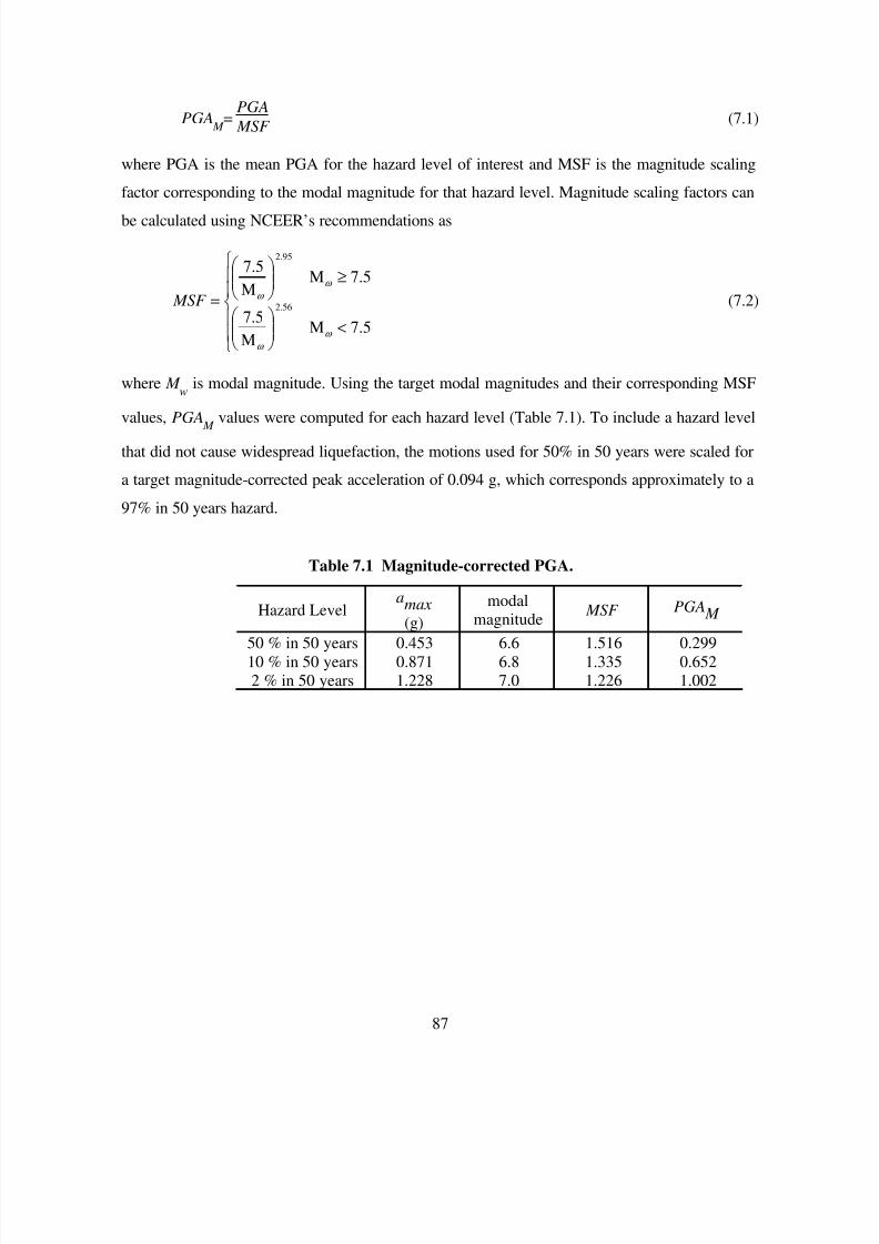
7/21/2019 PEER807 KRAMERArduino Shin
http://slidepdf.com/reader/full/peer807-kramerarduino-shin 100/198
87
PGA M
=PGA
MSF (7.1)
where PGA is the mean PGA for the hazard level of interest and MSF is the magnitude scaling
factor corresponding to the modal magnitude for that hazard level. Magnitude scaling factors can
be calculated using NCEER’s recommendations as
7.5<Μ
Μ
7.5
7.5≥Μ
Μ
7.5
= 2.56
2.95
ω
ω
ω
ω MSF (7.2)
where M w
is modal magnitude. Using the target modal magnitudes and their corresponding MSF
values, PGA M values were computed for each hazard level (Table 7.1). To include a hazard level
that did not cause widespread liquefaction, the motions used for 50% in 50 years were scaled for
a target magnitude-corrected peak acceleration of 0.094 g, which corresponds approximately to a
97% in 50 years hazard.
Table 7.1 Magnitude-corrected PGA.
Hazard Levelamax
(g)
modal
magnitude
MSF PGA M
50 % in 50 years 0.453 6.6 1.516 0.29910 % in 50 years 0.871 6.8 1.335 0.6522 % in 50 years 1.228 7.0 1.226 1.002

7/21/2019 PEER807 KRAMERArduino Shin
http://slidepdf.com/reader/full/peer807-kramerarduino-shin 101/198
88
Ten motions were selected for each hazard level. Individual motions were scaled to have
the target magnitude-corrected peak acceleration in each hazard. The values are presented in the
7th column (i.e., PGA M
) in Table 7.2.
Since the scaled motions were based on rock outcrop conditions, the motions werecorrected using the computer program ProShake to remove free surface effects prior to their use
as rigid base input motions in OpenSees. Information for the 40 motions is summarized in Table
7.2. Figure 7.2 shows the range of PGAs for each hazard level and the corresponding PGA
hazard curve.
Table 7.2 I-880 Input motion characteristics (four hazards).
hazard level Record
(station)
File Earthquake Magnitude MSF PGA M
dt PGA duration
Coyote LakeDam abutment
A01 Coyote Lake 5.7 2.247 0.672 0.005 0.574 40.96
Gilroy #6 A02 (6/ 8/1979) 0.005 0.610 40.96Temblor A03 Parkfield 6.0 1.931 0.578 0.010 0.469 40.96Array #5 A04 (6/27/1966) 0.010 0.470 81.92
Array #8 A05 0.010 0.394 40.96
FagundesRanch
A06 Livermore 5.5 2.497 0. 747 0.005 0.606 20.4 8
Morgan
Territory Park
A07 (6/27/1980) 0.005 0.483 40.96
Coyote Lake
Dam abutment
A08 Morgan Hill 6.2 1.753 0.524 0.005 0.423 40.96
returnperiod72 yrs
targetPGA
M
= 0.299g
Anderson Dam
DS
A09 (4/24/1984) 0.005 0.435 40.96
Halls Valley A10 0.005 0.464 40.96
Los GatosPresentationCtr
B01 Loma Prieta 7.0 1.226 0.799 0.005 0.687 40.96
Saratoga
Aloha Avenue
B02 (10/17/1989) 0.005 0.728 40.96
Corralitos B03 0.005 0.709 40.96Gavilan
College
B04 0.005 0.699 40.96
Gilroy Historic B05 0.005 0.691 40.96
LexingtonDam abutment
B06 0.020 0.759 40.96
Kobe JMA B07 Kobe, Japan 6.9 1.279 0.834 0.020 0.781 81.92( 1/17/1995)Kofu B08 Tottori, Japan 6.6 1.458 0.951 0.010 0.622 40.96
Hino B09 (10/6/2000) 0.005 0.897 81.92
return
period
475 yrs
target
PGA M
= 0.652g
Erzincan B10 Erzincan 6.7 1.395 0.909 0.005 0.696 40.96( 3/13/1992)
Los Gatos
Presentation
Ctr
C01 Loma Prieta 7.0 1.226 1.228 0.005 1.101 40.96
SaratogaAloha Avenue
C02 (10/17/1989) 0.005 1.141 40.96
Corralitos C03 0.005 1.078 40.96
GavilanCollege
C04 0.005 1.055 40.96
Gilroy Historic C05 0.005 1.063 40.96
LexingtonDam abutment
C06 0.020 1.191 40.96
Kobe JMA C07 Kobe, Japan 6.9 1.279 1.282 0.020 1.221 81.92
( 1/17/1995)
Kofu C08 Tottori, Japan 6.6 1.458 1.461 0.010 1.092 40.96Hino C09 (10/6/2000) 0.005 1.399 81.92
returnperiod
2475 yrs
targetPGA
M
= 1.002g
Erzincan C10 Erzincan,Turk
ey
6.7 1.395 1.398 0.005 1.107 40.96
( 3/13/1992)
Coyote LakeDam abutment D01 Coyote Lake 5.7 2.247 0.211 0.005 0.168 40.96
Gilroy #6 D02 (6/ 8/1979) 0.005 0.167 40.96Temblor D03 Parkfield 6.0 1.931 0.182 0.010 0.157 40.96
Array #5 D04 (6/27/1966) 0.010 0.137 81.92Array #8 D05 0.010 0.119 40.96
FagundesRanch
D06 Livermore 5.5 2.497 0. 235 0.005 0.189 20.4 8
Morgan
Territory Park
D07 (6/27/1980) 0.005 0.148 40.96
Coyote Lake
Dam abutment
D08 Morgan Hill 6.2 1.753 0.165 0.005 0.122 40.96
Anderson Dam
DS
D09 (4/24/1984) 0.005 0.126 40.96
return
period15 yrs
target
PGA M
= 0.094g
Halls Valley D10 0.005 0.124 40.96
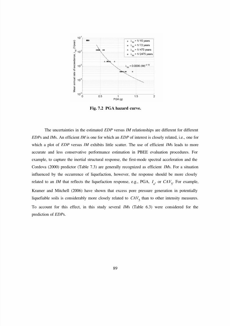
7/21/2019 PEER807 KRAMERArduino Shin
http://slidepdf.com/reader/full/peer807-kramerarduino-shin 102/198
89
Fig. 7.2 PGA hazard curve.
The uncertainties in the estimated EDP versus IM relationships are different for different
EDPs and IM s. An efficient IM is one for which an EDP of interest is closely related, i.e., one for
which a plot of EDP versus IM exhibits little scatter. The use of efficient IM s leads to more
accurate and less conservative performance estimation in PBEE evaluation procedures. For
example, to capture the inertial structural response, the first-mode spectral acceleration and the
Cordova (2000) predictor (Table 7.3) are generally recognized as efficient IM s. For a situation
influenced by the occurrence of liquefaction, however, the response should be more closely
related to an IM that reflects the liquefaction response, e.g., PGA, I a, or CAV
5. For example,
Kramer and Mitchell (2006) have shown that excess pore pressure generation in potentially
liquefiable soils is considerably more closely related to CAV 5 than to other intensity measures.
To account for this effect, in this study several IM s (Table 6.3) were considered for the
prediction of EDPs.
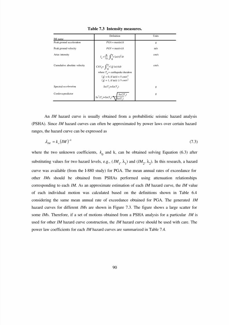
7/21/2019 PEER807 KRAMERArduino Shin
http://slidepdf.com/reader/full/peer807-kramerarduino-shin 103/198
90
Table 7.3 Intensity measures.
IM nameDefinition Units
Peak ground acceleration PGA = max|a(t )| g
Peak ground velocity PGV = max|v(t )| m/s
Arias intensity I a = π
2g ⌡⌠ 0
T d [a(t )]2 dt cm/s
Cumulative absolute velocityCAV
5=⌡⌠ 0
T d ⟨ χ⟩ |a(t )|dt
cm/s
where T d = earthquake duration
⟨ χ⟩ = 0, if |a(t)| < 5 cm/s2
⟨ χ⟩ = 1, if |a(t)| ≥ 5 cm/s2
Spectral acceleration Sa(T 1)=Sa(T
1) g
Cordova predictor
Sa*(T 1)=Sa(T
1)
Sa(2T 1)
Sa(T 1)
g
An IM hazard curve is usually obtained from a probabilistic seismic hazard analysis
(PSHA). Since IM hazard curves can often be approximated by power laws over certain hazard
ranges, the hazard curve can be expressed as
( ) k
o IM IM k −
=λ (7.3)
where the two unknown coefficients, k 0 and k, can be obtained solving Equation (6.3) after
substituting values for two hazard levels, e.g., ( IM 1, λ 1) and ( IM 2, λ 2). In this research, a hazard
curve was available (from the I-880 study) for PGA. The mean annual rates of exceedance for
other IM s should be obtained from PSHAs performed using attenuation relationships
corresponding to each IM . As an approximate estimation of each IM hazard curve, the IM value
of each individual motion was calculated based on the definitions shown in Table 6.4
considering the same mean annual rate of exceedance obtained for PGA. The generated IM
hazard curves for different IM s are shown in Figure 7.3. The figure shows a large scatter for
some IM s. Therefore, if a set of motions obtained from a PSHA analysis for a particular IM is
used for other IM hazard curve construction, the IM hazard curve should be used with care. The
power law coefficients for each IM hazard curves are summarized in Table 7.4.
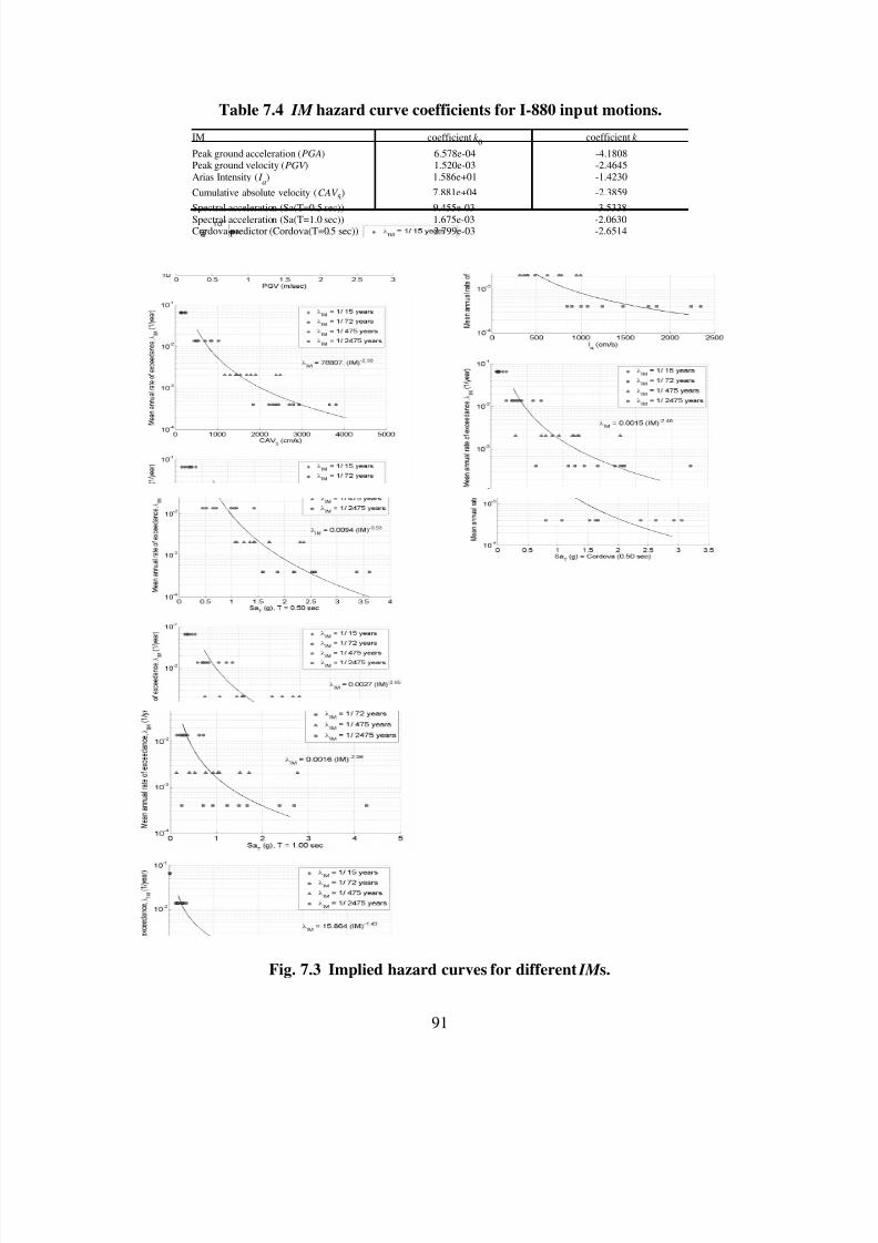
7/21/2019 PEER807 KRAMERArduino Shin
http://slidepdf.com/reader/full/peer807-kramerarduino-shin 104/198
91
Table 7.4 IM hazard curve coefficients for I-880 input motions.
IM coefficient k 0 coefficient k
Peak ground acceleration (PGA) 6.578e-04 -4.1808Peak ground velocity (PGV ) 1.520e-03 -2.4645Arias Intensity ( I
a) 1.586e+01 -1.4230
Cumulative absolute velocity (CAV 5) 7.881e+04 -2.3859
Spectral acceleration (Sa(T=0.5 sec)) 9.455e-03 -3.5338Spectral acceleration (Sa(T=1.0 sec)) 1.675e-03 -2.0630Cordova predictor (Cordova(T=0.5 sec)) 2.799e-03 -2.6514
Fig. 7.3 Implied hazard curves for different IM s.

7/21/2019 PEER807 KRAMERArduino Shin
http://slidepdf.com/reader/full/peer807-kramerarduino-shin 105/198
92
7.2.2 EDPs of Bridge System
By examining the bridge behavior from multiple numerical analyses, important EDPs (such as
maximum and residual values of bridge pier drift, horizontal slope movement, embankment
settlement, relative displacement between bridge deck and abutment approach, pile cap
movement, and pile curvature) were identified. A list of possible EDPs for the bridge system is
shown in Table 7.5.
Table 7.5 EDP list.
EDP
group EDP
description EDP
symbolDefinition
C 1[drift,max]
C 2[drift,max]
C 3[drift,max]
column drift ratio
C 4[drift,max]
maximum drift ratio = maximumdrift/column height
P0[drift,res]
P1[drift,res]
P2[drift,res]
P3[drift,res]
P4[drift,res]
pile cappile cap drift
(displacement)
P5[drift,res]
permanent lateral displacement ofpile cap
EJ 1[gap,res]
abutment expansion joint
gap betweendeck and abutment EJ 2
[gap,res]
relative distance between deck endand break-off wall
BW 1[dx,max]
abutment backwall
backwalldisplacement BW 2
[dx,max]
break-off wall displacement = disp.of bearing pad spring - initial gap
BA1[dy,res]
abutment approach
bridge approachvert. off-set BA2
[dy,res]
relative vertical displacementbetween abutment top and adjacent
backfill soil BP1
[dx,max]
bearing padbearing pad
displacement BP2[dx,max]
maximum relative lateraldisplacement between deck and
stem wall
E 1[dx,res]
E 2[dx,res]
lateral disp.settlement
E 1[dy,res]
embankment slope
E 2[dy,res]
average lateral displacement ofslope top and toe average verticaldisplacement of slope top and toe
The list divides EDPs into several groups that can be associated with structural and
geotechnical damage and cost estimation. The structural EDP groups include column drift,
expansion joint displacement, bridge approach vertical off-set, break-off wall displacement, and
bearing pad shear strain. The structural EDPs were selected to be consistent with the EDP groups
used by Mackie et al. (2004), who performed similar analyses using the same bridge model on
competent soil. Abutment slope deformation and pile cap displacement were included as new
geotechnical EDP groups. Even though the actual damage to a pile is most closely related to pile
bending moment or curvature, these EDPs may not be practical for estimation of damage, since
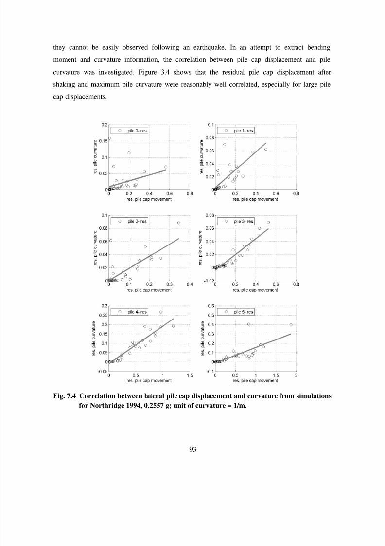
7/21/2019 PEER807 KRAMERArduino Shin
http://slidepdf.com/reader/full/peer807-kramerarduino-shin 106/198
93
they cannot be easily observed following an earthquake. In an attempt to extract bending
moment and curvature information, the correlation between pile cap displacement and pile
curvature was investigated. Figure 3.4 shows that the residual pile cap displacement after
shaking and maximum pile curvature were reasonably well correlated, especially for large pile
cap displacements.
Fig. 7.4 Correlation between lateral pile cap displacement and curvature from simulations
for Northridge 1994, 0.2557 g; unit of curvature = 1/m.
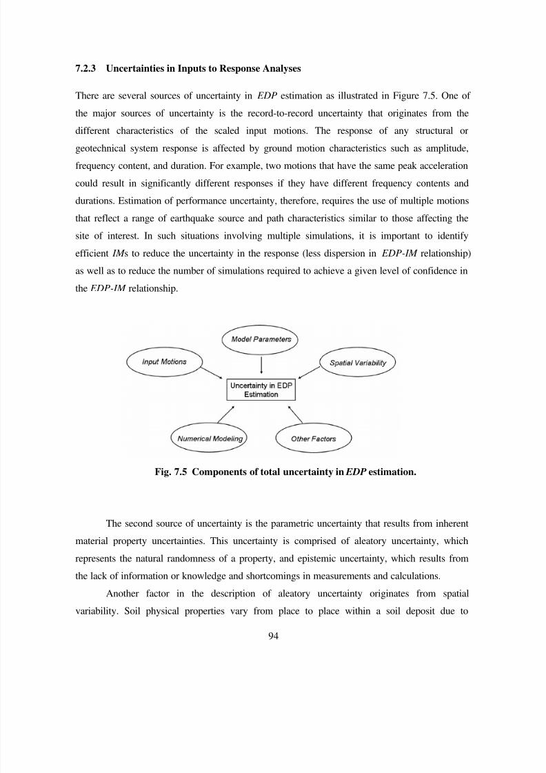
7/21/2019 PEER807 KRAMERArduino Shin
http://slidepdf.com/reader/full/peer807-kramerarduino-shin 107/198
94
7.2.3 Uncertainties in Inputs to Response Analyses
There are several sources of uncertainty in EDP estimation as illustrated in Figure 7.5. One of
the major sources of uncertainty is the record-to-record uncertainty that originates from the
different characteristics of the scaled input motions. The response of any structural or
geotechnical system response is affected by ground motion characteristics such as amplitude,
frequency content, and duration. For example, two motions that have the same peak acceleration
could result in significantly different responses if they have different frequency contents and
durations. Estimation of performance uncertainty, therefore, requires the use of multiple motions
that reflect a range of earthquake source and path characteristics similar to those affecting the
site of interest. In such situations involving multiple simulations, it is important to identify
efficient IM s to reduce the uncertainty in the response (less dispersion in EDP-IM relationship)as well as to reduce the number of simulations required to achieve a given level of confidence in
the EDP-IM relationship.
Fig. 7.5 Components of total uncertainty in EDP estimation.
The second source of uncertainty is the parametric uncertainty that results from inherent
material property uncertainties. This uncertainty is comprised of aleatory uncertainty, which
represents the natural randomness of a property, and epistemic uncertainty, which results from
the lack of information or knowledge and shortcomings in measurements and calculations.
Another factor in the description of aleatory uncertainty originates from spatial
variability. Soil physical properties vary from place to place within a soil deposit due to
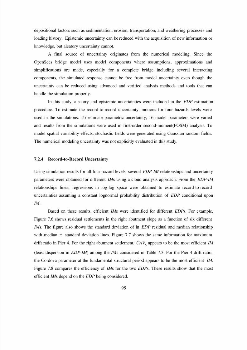
7/21/2019 PEER807 KRAMERArduino Shin
http://slidepdf.com/reader/full/peer807-kramerarduino-shin 108/198
95
depositional factors such as sedimentation, erosion, transportation, and weathering processes and
loading history. Epistemic uncertainty can be reduced with the acquisition of new information or
knowledge, but aleatory uncertainty cannot.
A final source of uncertainty originates from the numerical modeling. Since the
OpenSees bridge model uses model components where assumptions, approximations and
simplifications are made, especially for a complete bridge including several interacting
components, the simulated response cannot be free from model uncertainty even though the
uncertainty can be reduced using advanced and verified analysis methods and tools that can
handle the simulation properly.
In this study, aleatory and epistemic uncertainties were included in the EDP estimation
procedure. To estimate the record-to-record uncertainty, motions for four hazards levels were
used in the simulations. To estimate parametric uncertainty, 16 model parameters were varied
and results from the simulations were used in first-order second-moment(FOSM) analysis. To
model spatial variability effects, stochastic fields were generated using Gaussian random fields.
The numerical modeling uncertainty was not explicitly evaluated in this study.
7.2.4 Record-to-Record Uncertainty
Using simulation results for all four hazard levels, several EDP-IM relationships and uncertainty
parameters were obtained for different IM s using a cloud analysis approach. From the EDP- IM
relationships linear regressions in log-log space were obtained to estimate record-to-record
uncertainties assuming a constant lognormal probability distribution of EDP conditional upon
IM .
Based on these results, efficient IM s were identified for different EDPs. For example,
Figure 7.6 shows residual settlements in the right abutment slope as a function of six different
IM s. The figure also shows the standard deviation of ln EDP residual and median relationship
with median ± standard deviation lines. Figure 7.7 shows the same information for maximum
drift ratio in Pier 4. For the right abutment settlement, CAV 5 appears to be the most efficient IM
(least dispersion in EDP- IM ) among the IM s considered in Table 7.3. For the Pier 4 drift ratio,
the Cordova parameter at the fundamental structural period appears to be the most efficient IM .
Figure 7.8 compares the efficiency of IM s for the two EDPs. These results show that the most
efficient IM s depend on the EDP being considered.
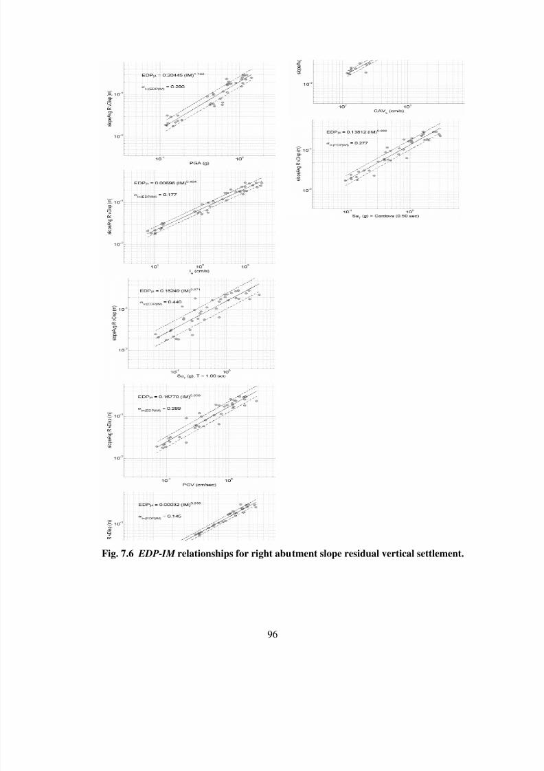
7/21/2019 PEER807 KRAMERArduino Shin
http://slidepdf.com/reader/full/peer807-kramerarduino-shin 109/198
96
Fig. 7.6 EDP- IM relationships for right abutment slope residual vertical settlement.
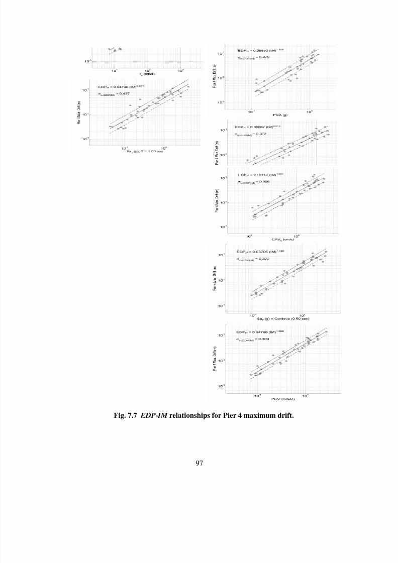
7/21/2019 PEER807 KRAMERArduino Shin
http://slidepdf.com/reader/full/peer807-kramerarduino-shin 110/198
97
Fig. 7.7 EDP- IM relationships for Pier 4 maximum drift.
7/21/2019 PEER807 KRAMERArduino Shin
http://slidepdf.com/reader/full/peer807-kramerarduino-shin 111/198
98
Fig. 7.8 Relative efficiencies of different IM s.
Using EDP- IM results, record-to-record uncertainties and median EDP- IM relationships
were obtained for several EDP groups. The results are summarized in Table 7.6 where the
corresponding efficient IM s are indicated. This summary table shows that CAV 5 is one of the
most efficient IM s for the EDPs affected by lateral spreading such as slope deformation,
abutment expansion joint movement, and pile cap lateral movement near slopes, while spectral
acceleration or PGV is more efficient for structural related EDPs such as bridge pier drift ratio.
Overall, residual EDPs obtained at the end of shaking showed higher uncertainty than maximum
EDPs. Pile cap displacements also showed higher uncertainty than bridge pier drifts.
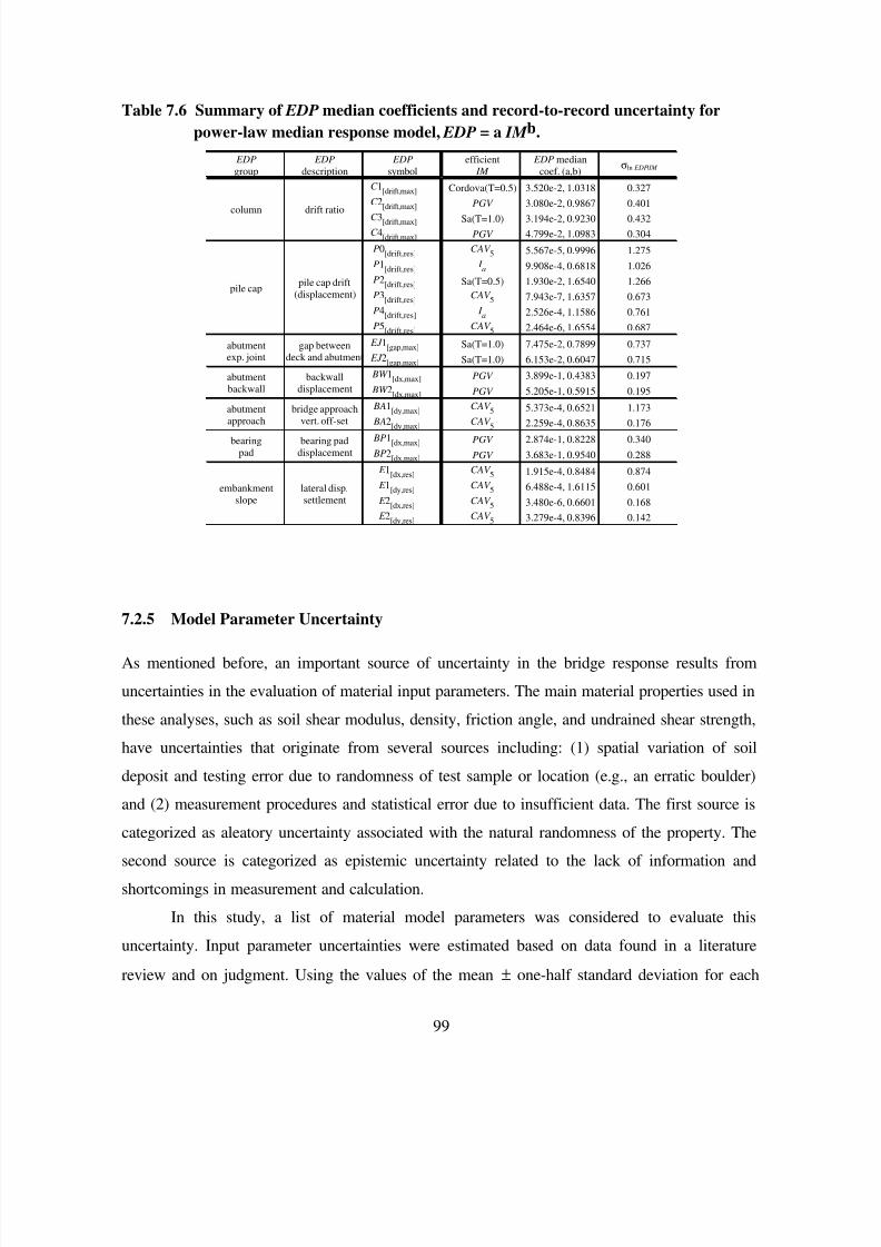
7/21/2019 PEER807 KRAMERArduino Shin
http://slidepdf.com/reader/full/peer807-kramerarduino-shin 112/198
99
Table 7.6 Summary of EDP median coefficients and record-to-record uncertainty for
power-law median response model, EDP = a IM b.
EDP
group
EDP
description
EDP
symbol
efficient IM
EDP median
coef. (a,b)σln EDP| IM
C 1[drift,max]
Cordova(T=0.5) 3.520e-2, 1.0318 0.327
C 2[drift,max]
PGV 3.080e-2, 0.9867 0.401
C 3[drift,max]
Sa(T=1.0) 3.194e-2, 0.9230 0.432column drift ratio
C 4[drift,max]
PGV 4.799e-2, 1.0983 0.304
P0[drift,res]
CAV 5 5.567e-5, 0.9996 1.275
P1[drift,res]
I a 9.908e-4, 0.6818 1.026
P2[drift,res]
Sa(T=0.5) 1.930e-2, 1.6540 1.266
P3[drift,res]
CAV 5 7.943e-7, 1.6357 0.673
P4[drift,res]
I a 2.526e-4, 1.1586 0.761
pile cappile cap drift
(displacement)
P5[drift,res]
CAV 5 2.464e-6, 1.6554 0.687
EJ 1[gap,max]
Sa(T=1.0) 7.475e-2, 0.7899 0.737abutmentexp. joint
gap betweendeck and abutment EJ 2
[gap,max] Sa(T=1.0) 6.153e-2, 0.6047 0.715
BW 1[dx,max]
PGV 3.899e-1, 0.4383 0.197abutment
backwall
backwall
displacement BW 2[dx,max]
PGV 5.205e-1, 0.5915 0.195
BA1[dy,max]
CAV 5 5.373e-4, 0.6521 1.173abutment
approach
bridge approach
vert. off-set BA2[dy,max]
CAV 5 2.259e-4, 0.8635 0.176
BP1[dx,max]
PGV 2.874e-1, 0.8228 0.340bearing
pad
bearing pad
displacement BP2[dx,max]
PGV 3.683e-1, 0.9540 0.288
E 1[dx,res]
CAV 5 1.915e-4, 0.8484 0.874
E 1[dy,res]
CAV 5 6.488e-4, 1.6115 0.601
E 2[dx,res]
CAV 5 3.480e-6, 0.6601 0.168
embankment
slope
lateral disp.
settlement
E 2[dy,res]
CAV 5 3.279e-4, 0.8396 0.142
7.2.5 Model Parameter Uncertainty
As mentioned before, an important source of uncertainty in the bridge response results from
uncertainties in the evaluation of material input parameters. The main material properties used in
these analyses, such as soil shear modulus, density, friction angle, and undrained shear strength,
have uncertainties that originate from several sources including: (1) spatial variation of soil
deposit and testing error due to randomness of test sample or location (e.g., an erratic boulder)
and (2) measurement procedures and statistical error due to insufficient data. The first source is
categorized as aleatory uncertainty associated with the natural randomness of the property. The
second source is categorized as epistemic uncertainty related to the lack of information and
shortcomings in measurement and calculation.
In this study, a list of material model parameters was considered to evaluate this
uncertainty. Input parameter uncertainties were estimated based on data found in a literature
review and on judgment. Using the values of the mean ± one-half standard deviation for each
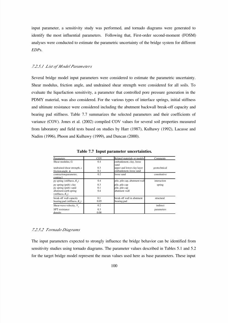
7/21/2019 PEER807 KRAMERArduino Shin
http://slidepdf.com/reader/full/peer807-kramerarduino-shin 113/198
100
input parameter, a sensitivity study was performed, and tornado diagrams were generated to
identify the most influential parameters. Following that, First-order second-moment (FOSM)
analyses were conducted to estimate the parametric uncertainty of the bridge system for different
EDPs.
7.2.5.1 L ist of Model Param eters
Several bridge model input parameters were considered to estimate the parametric uncertainty.
Shear modulus, friction angle, and undrained shear strength were considered for all soils. To
evaluate the liquefaction sensitivity, a parameter that controlled pore pressure generation in the
PDMY material, was also considered. For the various types of interface springs, initial stiffness
and ultimate resistance were considered including the abutment backwall break-off capacity andbearing pad stiffness. Table 7.7 summarizes the selected parameters and their coefficients of
variance (COV). Jones et al. (2002) compiled COV values for several soil properties measured
from laboratory and field tests based on studies by Harr (1987), Kulhawy (1992), Lacasse and
Nadim (1996), Phoon and Kulhawy (1999), and Duncan (2000).
Table 7.7 Input parameter uncertainties.
Parameters COV Related materials or models Comments
Shear modulus, G 0.4 embankment, clay, loosesand
undrained shear strength, c 0.3 upper and lower clay layer geotechnical
friction angle, φ 0.1 embankment, loose sand
contraction parameter,contrac1
0.2 loose sand constitutive
py spring (stiffness,K 1) 0.4 pile, pile cap, abutment wall interaction
py spring (pult): clay 0.3 pile, pile cap springpy spring (pult): sand 0.1 pile, pile capabutment earth spring(stiffness,K
2)
0.4 abutment wall
break-off wall capacity 0.1 break-off wall in abutment structuralbearing pad (stiffness,K
3) 0.05 bearing pad
Shear wave velocity, V s 0.2 indirect
SPT resistance 0.3 parametersdensity 0.08
7.2.5.2 Tornado Diagrams
The input parameters expected to strongly influence the bridge behavior can be identified from
sensitivity studies using tornado diagrams. The parameter values described in Tables 5.1 and 5.2
for the target bridge model represent the mean values used here as base parameters. These input
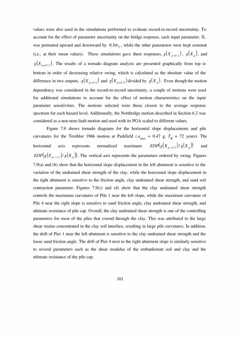
7/21/2019 PEER807 KRAMERArduino Shin
http://slidepdf.com/reader/full/peer807-kramerarduino-shin 114/198
101
values were also used in the simulations performed to evaluate record-to-record uncertainty. To
account for the effect of parameter uncertainty on the bridge response, each input parameter, X,
was permuted upward and downward by X σ 5.0 , while the other parameters were kept constant
(i.e., at their mean values). These simulations gave three responses,2 / σ µ −
X g , µ
X g , and
( )2 / σ µ + X g . The results of a tornado diagram analysis are presented graphically from top to
bottom in order of decreasing relative swing, which is calculated as the absolute value of the
difference in two outputs, 2 / σ µ − X g and 2 / σ µ + X g divided by µ X g . Even though the motion
dependency was considered in the record-to-record uncertainty, a couple of motions were used
for additional simulations to account for the effect of motion characteristics on the input
parameter sensitivities. The motions selected were those closest to the average response
spectrum for each hazard level. Additionally, the Northridge motion described in Section 6.2 was
considered as a non-near-fault motion and used with its PGA scaled to different values.
Figure 7.9 shows tornado diagrams for the horizontal slope displacements and pile
curvatures for the Temblor 1966 motion at Parkfield (amax
= 0.47 g, T R
= 72 years). The
horizontal axis represents normalized maximum µ σ µ X g X g EDP / 2 / − and
( ) ( )( ) µ µ X g X g EDP / 2 / +− . The vertical axis represents the parameters ordered by swing. Figures
7.9(a) and (b) show that the horizontal slope displacement in the left abutment is sensitive to the
variation of the undrained shear strength of the clay, while the horizontal slope displacement in
the right abutment is sensitive to the friction angle, clay undrained shear strength, and sand soil
contraction parameter. Figures 7.9(c) and (d) show that the clay undrained shear strength
controls the maximum curvatures of Pile 1 near the left slope, while the maximum curvature of
Pile 4 near the right slope is sensitive to sand friction angle, clay undrained shear strength, and
ultimate resistance of pile cap. Overall, the clay undrained shear strength is one of the controlling
parameters for most of the piles that extend through the clay. This was attributed to the large
shear strains concentrated in the clay soil interface, resulting in large pile curvatures. In addition,
the drift of Pier 1 near the left abutment is sensitive to the clay undrained shear strength and the
loose sand friction angle. The drift of Pier 4 next to the right abutment slope is similarly sensitive
to several parameters such as the shear modulus of the embankment soil and clay and the
ultimate resistance of the pile cap.
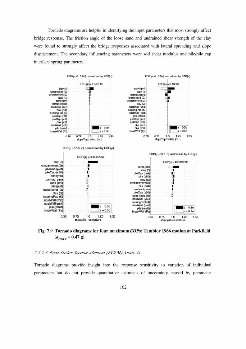
7/21/2019 PEER807 KRAMERArduino Shin
http://slidepdf.com/reader/full/peer807-kramerarduino-shin 115/198
102
Tornado diagrams are helpful in identifying the input parameters that most strongly affect
bridge response. The friction angle of the loose sand and undrained shear strength of the clay
were found to strongly affect the bridge responses associated with lateral spreading and slope
displacement. The secondary influencing parameters were soil shear modulus and pile/pile cap
interface spring parameters.
Fig. 7.9 Tornado diagrams for four maximum EDPs: Temblor 1966 motion at Parkfield
( a max
= 0.47 g).
7.2.5.3 First-Order Second-Moment (FOSM) Analysis
Tornado diagrams provide insight into the response sensitivity to variation of individual
parameters but do not provide quantitative estimates of uncertainty caused by parameter
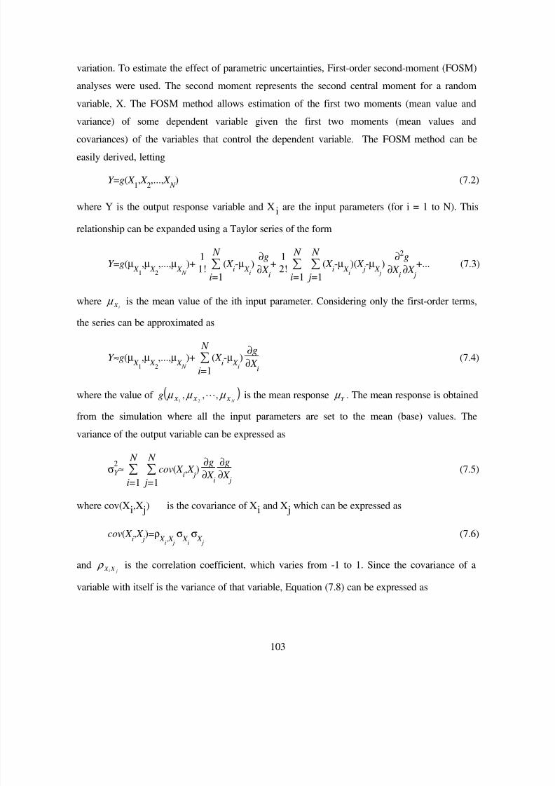
7/21/2019 PEER807 KRAMERArduino Shin
http://slidepdf.com/reader/full/peer807-kramerarduino-shin 116/198
103
variation. To estimate the effect of parametric uncertainties, First-order second-moment (FOSM)
analyses were used. The second moment represents the second central moment for a random
variable, X. The FOSM method allows estimation of the first two moments (mean value and
variance) of some dependent variable given the first two moments (mean values and
covariances) of the variables that control the dependent variable. The FOSM method can be
easily derived, letting
Y =g( X 1, X
2,..., X
N ) (7.2)
where Y is the output response variable and Xi are the input parameters (for i = 1 to N). This
relationship can be expanded using a Taylor series of the form
Y =g(µ X 1,µ X
2,...,µ X
N )+
1
1! ∑i=1
N
( X i-µ X i)
∂g
∂ X i+
1
2! ∑i=1
N
∑ j=1
N
( X i-µ X i)( X j-µ X
j)
∂2g
∂ X i ∂ X
j+... (7.3)
wherei X µ is the mean value of the ith input parameter. Considering only the first-order terms,
the series can be approximated as
Y ≈g(µ X
1
,µ X
2
,...,µ X
N
)+ ∑i=1
N
( X i-µ
X i
)∂g
∂ X i
(7.4)
where the value of N X X X g µ µ µ ,,, 21
is the mean response Y µ . The mean response is obtained
from the simulation where all the input parameters are set to the mean (base) values. The
variance of the output variable can be expressed as
σ2
Y ≈ ∑i=1
N
∑ j=1
N
cov( X i, X
j)
∂g
∂ X i
∂g
∂ X j
(7.5)
where cov(Xi,X j) is the covariance of Xi and X j which can be expressed as
cov( X i, X
j)=ρ
X i, X
j
σ X
i
σ X
j
(7.6)
and ji X X ρ is the correlation coefficient, which varies from -1 to 1. Since the covariance of a
variable with itself is the variance of that variable, Equation (7.8) can be expressed as

7/21/2019 PEER807 KRAMERArduino Shin
http://slidepdf.com/reader/full/peer807-kramerarduino-shin 117/198
104
σ2
Y ≈ ∑i=1
N
σ2
X i (
∂g
∂ X i
)2 + ∑
i=1
N
∑ j≠i
N
ρ X
i, X
j
σ X
i
σ X
j
∂g
∂ X i
∂g
∂ X j
(7.7)
In this work gradients were approximated numerically by central differences over a range
of 2 / ii X X σ µ − to 2 /
ii X X σ µ + for each variable; the values of the correlation coefficients
( ji X X ρ ) between input parameters were approximated as shown in Table 7.8. These values were
determined approximately considering possible correlations with judgment. Most of the
correlation coefficients between soil and structural parameters were set to zero.
Table 7.8 Correlation coefficients for uncertain input parameters.
EDP uncertainties were obtained based on Equation (6.10) using simulation results using
four input motions. The estimated uncertainties for each EDP are presented in Table 7.9.

7/21/2019 PEER807 KRAMERArduino Shin
http://slidepdf.com/reader/full/peer807-kramerarduino-shin 118/198
105
Table 7.9 Summary of parametric uncertainty.
σln(EDP|IM) σln(EDP|IM)
EDP
symbol
Northridge
(0.1g)
Northridge
(0.25g)
A03
(0.46g)
B10
(0.70g)average
C 1[drift,max]
0.018 0.040 0.401 0.075 0.134
C 2[drift,max] 0.023 0.025 0.024 0.044 0.031
C 3[drift,max]
0.013 0.042 0.029 0.042 0.031
C 4[drift,max]
0.008 0.052 0.042 0.076 0.045
P0[drift,res]
0.062 0.064 0.090 0.056 0.068
P1[drift,res]
0.118 0.344 0.588 0.082 0.283
P2[drift,res]
0.784 0.060 0.041 0.653 0.384
P3[drift,res]
0.288 0.051 0.042 0.095 0.119
P4[drift,res]
0.219 0.035 0.029 0.065 0.087
P5[drift,res]
0.236 0.086 0.047 0.049 0.105
EJ 1[gap,max]
0.346 0.031 0.070 0.074 0.130
EJ 2[gap,max]
0.695 0.121 0.075 0.100 0.248
BW 1[dx,max]
0.016 0.027 0.022 0.051 0.029
BW 2[dx,max]
0.010 0.012 0.018 0.056 0.024
BA1[dy,max]
0.020 0.039 0.025 0.055 0.035
BA2[dy,max]
0.040 0.066 0.043 0.084 0.058
BP1[dx,max]
0.346 0.031 0.070 0.074 0.130
BP2[dx,max]
0.695 0.121 0.075 0.100 0.248
E 1[dx,res]
0.059 0.067 0.081 0.054 0.065
E 2[dx,res]
0.019 0.034 0.022 0.049 0.031
E 1[dy,res]
0.227 0.080 0.047 0.048 0.101
E 2[dy,res]
0.035 0.063 0.039 0.080 0.054
7.2.6 Spatial Variability Effects
To investigate the spatial variability uncertainty, Gaussian stochastic random fields were
generated for the clay and liquefiable soil layers by randomizing the assigned soil strength
parameter over the soil layers with a certain spatial correlation. This section briefly describes the
method used to develop the stochastic fields and presents the estimated bridge response
uncertainty values due to spatial variability. For this purpose 10 random field simulations were
performed for several earthquake motions.
7.2.6.1
Spatial V ariability within Homogeneous Soil Deposits
The physical properties of soils vary from place to place within a soil deposit due to varying
geologic formation and loading histories such as sedimentation, erosion, transportation, and
weathering processes. This spatial variability in the soil properties cannot be simply described by
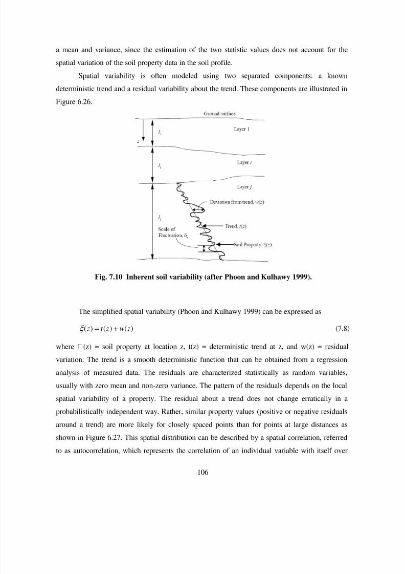
7/21/2019 PEER807 KRAMERArduino Shin
http://slidepdf.com/reader/full/peer807-kramerarduino-shin 119/198
106
a mean and variance, since the estimation of the two statistic values does not account for the
spatial variation of the soil property data in the soil profile.
Spatial variability is often modeled using two separated components: a known
deterministic trend and a residual variability about the trend. These components are illustrated in
Figure 6.26.
Fig. 7.10 Inherent soil variability (after Phoon and Kulhawy 1999).
The simplified spatial variability (Phoon and Kulhawy 1999) can be expressed as
)()()( zw zt z +=ξ (7.8)
where (z) = soil property at location z, t(z) = deterministic trend at z, and w(z) = residual
variation. The trend is a smooth deterministic function that can be obtained from a regression
analysis of measured data. The residuals are characterized statistically as random variables,
usually with zero mean and non-zero variance. The pattern of the residuals depends on the local
spatial variability of a property. The residual about a trend does not change erratically in a
probabilistically independent way. Rather, similar property values (positive or negative residuals
around a trend) are more likely for closely spaced points than for points at large distances as
shown in Figure 6.27. This spatial distribution can be described by a spatial correlation, referred
to as autocorrelation, which represents the correlation of an individual variable with itself over
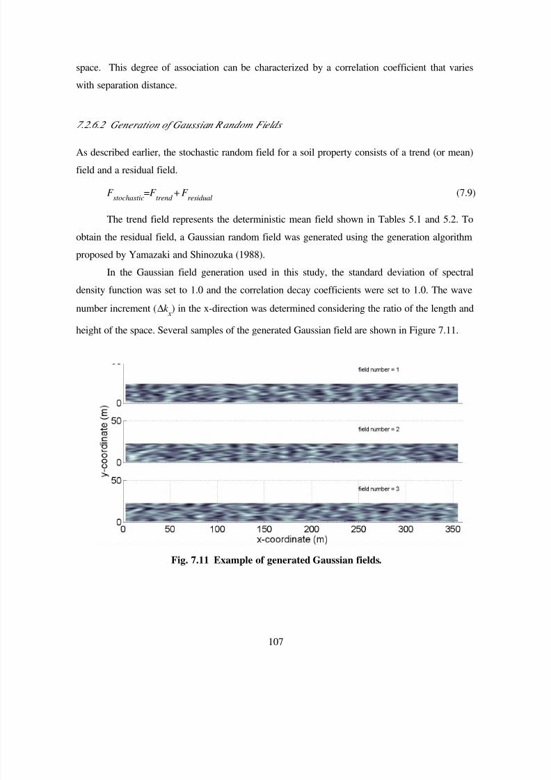
7/21/2019 PEER807 KRAMERArduino Shin
http://slidepdf.com/reader/full/peer807-kramerarduino-shin 120/198
107
space. This degree of association can be characterized by a correlation coefficient that varies
with separation distance.
7.2.6.2 Generation of Gaussian R andom Fields
As described earlier, the stochastic random field for a soil property consists of a trend (or mean)
field and a residual field.
F stochastic
=F trend
+ F residual
(7.9)
The trend field represents the deterministic mean field shown in Tables 5.1 and 5.2. To
obtain the residual field, a Gaussian random field was generated using the generation algorithm
proposed by Yamazaki and Shinozuka (1988).
In the Gaussian field generation used in this study, the standard deviation of spectral
density function was set to 1.0 and the correlation decay coefficients were set to 1.0. The wave
number increment (∆k x
) in the x-direction was determined considering the ratio of the length and
height of the space. Several samples of the generated Gaussian field are shown in Figure 7.11.
Fig. 7.11 Example of generated Gaussian fields.

7/21/2019 PEER807 KRAMERArduino Shin
http://slidepdf.com/reader/full/peer807-kramerarduino-shin 121/198
108
In the numerical simulation, since individual soil elements had different soil properties,
the stochastic random field was expressed in matrix form as
),(),(),(),(),(),( jiF jiF jiF jiF jiF jiF Gaussianmeanmeanresidualmeanstochastic +=+= (7.10)
where i and j represent the element position in the horizontal and vertical directions. F stochastic
is
a matrix of stochastic random fields for a soil property, F mean
is a matrix of deterministic mean
fields, COV is the coefficient of variance of the considered soil property, and F Gaussian
represents
the residual Gaussian field in matrix form. The dimension of the generated field matrix was the
same as that of the soil mesh used in the numerical simulations. That is, the rectangular soil
domain that includes loose sand and clay layers below the ground surface and above the dense
sand layer (i.e., layer 2, 3, and 4 in Fig. 4.1). The generated Gaussian field could not be directly
used in the simulation, since values in the field were calculated for uniform incremental positions
in the horizontal and vertical direction, whereas the soil mesh in the OpenSees model did not
have uniform element size. Therefore, the values obtained using Yamazaki and Shinozuka
(1988)’s method were interpolated according to the soil element center locations. The steps in
the random field generation procedure for the bridge analyses were as follows:
1. Generate mean field using mean target soil properties
2. Generate Gaussian random (autocorrelated) fields for φ and c in the loose sand and clay
layers with mean = 0.0 and σ = 1.0 : Yamazaki and Shinozuka (1988)
3. Normalize the Gaussian field by its maximum value
4. Interpolate the Gaussian field to the FEM mesh
5. Determine COV values for φ and c
6. Combine the mean field and Gaussian field to obtain a stochastic field using Equation
(7.12).
To illustrate the difference between deterministic and stochastic fields, a stochastic field
friction angle was considered for the loose sand layer. Figure 6.28 illustrates the mean, Gaussian,
and total friction angle parameter fields.
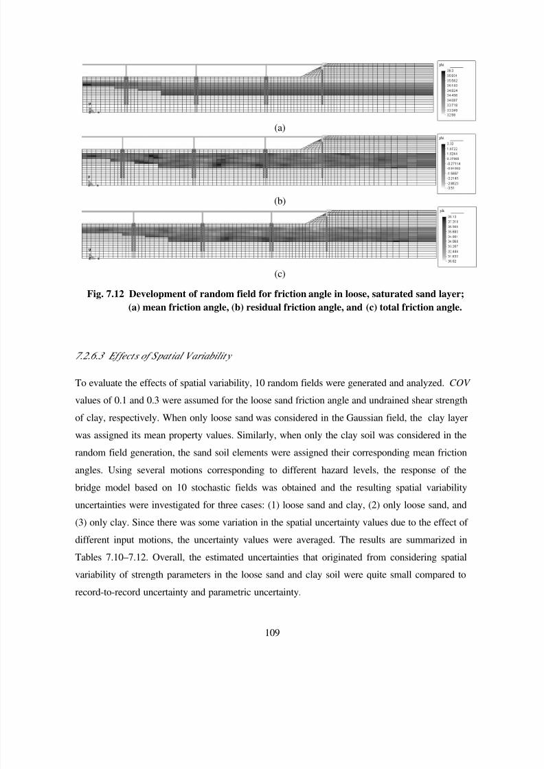
7/21/2019 PEER807 KRAMERArduino Shin
http://slidepdf.com/reader/full/peer807-kramerarduino-shin 122/198
109
(a)
(b)
(c)
Fig. 7.12 Development of random field for friction angle in loose, saturated sand layer;
(a) mean friction angle, (b) residual friction angle, and (c) total friction angle.
7.2.6.3 Ef fects of Spatial Variability
To evaluate the effects of spatial variability, 10 random fields were generated and analyzed. COV values of 0.1 and 0.3 were assumed for the loose sand friction angle and undrained shear strength
of clay, respectively. When only loose sand was considered in the Gaussian field, the clay layer
was assigned its mean property values. Similarly, when only the clay soil was considered in the
random field generation, the sand soil elements were assigned their corresponding mean friction
angles. Using several motions corresponding to different hazard levels, the response of the
bridge model based on 10 stochastic fields was obtained and the resulting spatial variability
uncertainties were investigated for three cases: (1) loose sand and clay, (2) only loose sand, and
(3) only clay. Since there was some variation in the spatial uncertainty values due to the effect of
different input motions, the uncertainty values were averaged. The results are summarized in
Tables 7.10–7.12. Overall, the estimated uncertainties that originated from considering spatial
variability of strength parameters in the loose sand and clay soil were quite small compared to
record-to-record uncertainty and parametric uncertainty.

7/21/2019 PEER807 KRAMERArduino Shin
http://slidepdf.com/reader/full/peer807-kramerarduino-shin 123/198
110
Table 7.10 Summary of spatial variability uncertainty (loose sand plus clay).
EDP
Northridge Northridge A03 B10 average
symbol (0.1g) (0.25g) (0.46g) (0.70g)
C 1[drift,max] 0.008 0.096 0.020 0.066 0.048C 2
[drift,max] 0.004 0.118 0.018 0.035 0.044
C 3[drift,max]
0.005 0.012 0.009 0.048 0.018
C 4[drift,max]
0.004 0.071 0.053 0.072 0.050
P0[drift,res]
0.053 0.059 0.052 0.085 0.062
P1[drift,res]
0.209 0.189 0.094 0.073 0.141
P2[drift,res]
0.108 0.188 0.067 0.488 0.213
P3[drift,res]
0.102 0.108 0.048 0.089 0.087
P4[drift,res]
0.098 0.075 0.049 0.032 0.064
P5[drift,res]
0.080 0.062 0.039 0.044 0.056
EJ 1[gap,max]
0.016 0.018 0.027 0.070 0.033
EJ 2[gap,max]
0.004 0.004 0.008 0.008 0.006
BW 1[dx,max]
0.002 0.005 0.005 0.019 0.008
BW 2[dx,max]
0.001 0.001 0.002 0.001 0.001
BA1[dy,max]
0.009 0.029 0.010 0.096 0.036
BA2[dy,max]
0.024 0.041 0.027 0.055 0.037
BP1[dx,max]
0.012 0.079 0.016 0.040 0.037
BP2[dx,max]
0.004 0.071 0.018 0.050 0.036
E 1[dx,res]
0.043 0.058 0.044 0.080 0.057
E 2[dx,res]
0.010 0.025 0.006 0.088 0.032
E 1[dy,res]
0.067 0.062 0.038 0.040 0.051
E 2[dy,res]
0.019 0.045 0.029 0.053 0.036

7/21/2019 PEER807 KRAMERArduino Shin
http://slidepdf.com/reader/full/peer807-kramerarduino-shin 124/198
111
Table 7.11 Summary of spatial variability uncertainty (loose sand).
EDP
Northridge Northridge A03 B10 average
symbol (0.1g) (0.25g) (0.46g) (0.70g)
C 1[drift,max]
0.003 0.019 0.015 0.026 0.016
C 2[drift,max]
0.002 0.013 0.014 0.019 0.012
C 3[drift,max] 0.003 0.008 0.007 0.011 0.007
C 4[drift,max]
0.002 0.056 0.054 0.057 0.042
P0[drift,res]
0.005 0.040 0.027 0.044 0.029
P1[drift,res]
0.123 0.070 0.081 0.036 0.077
P2[drift,res]
0.095 0.083 0.058 0.233 0.117
P3[drift,res]
0.094 0.045 0.042 0.075 0.064
P4[drift,res]
0.089 0.049 0.046 0.036 0.055
P5[drift,res]
0.076 0.056 0.043 0.019 0.048
EJ 1[gap,max]
0.003 0.004 0.030 0.002 0.010
EJ 2[gap,max]
0.001 0.002 0.005 0.002 0.002
BW 1[dx,max]
0.000 0.001 0.005 0.001 0.002
BW 2[dx,max]
0.000 0.000 0.001 0.000 0.000
BA1[dy,max]
0.002 0.029 0.005 0.040 0.019
BA2[dy,max] 0.023 0.035 0.029 0.046 0.033 BP1
[dx,max] 0.002 0.034 0.018 0.029 0.021
BP2[dx,max]
0.001 0.064 0.022 0.023 0.028
E 1[dx,res]
0.005 0.037 0.024 0.041 0.027
E 2[dx,res]
0.002 0.024 0.004 0.031 0.015
E 1[dy,res]
0.063 0.055 0.041 0.019 0.045
E 2[dy,res]
0.017 0.038 0.030 0.045 0.033
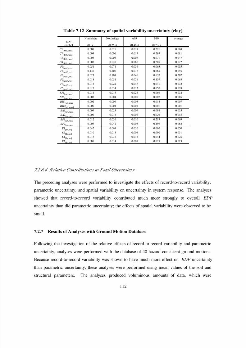
7/21/2019 PEER807 KRAMERArduino Shin
http://slidepdf.com/reader/full/peer807-kramerarduino-shin 125/198
112
Table 7.12 Summary of spatial variability uncertainty (clay).
EDP
Northridge Northridge A03 B10 average
symbol (0.1g) (0.25g) (0.46g) (0.70g)
C 1[drift,max]
0.008 0.025 0.019 0.221 0.068
C 2[drift,max]
0.003 0.006 0.017 0.299 0.081
C 3[drift,max] 0.003 0.006 0.008 0.071 0.047C 4
[drift,max] 0.003 0.020 0.060 0.205 0.072
P0[drift,res]
0.051 0.071 0.036 0.063 0.055
P1[drift,res]
0.130 0.106 0.078 0.065 0.095
P2[drift,res]
0.023 0.101 0.046 0.637 0.202
P3[drift,res]
0.018 0.051 0.026 0.159 0.063
P4[drift,res]
0.018 0.022 0.047 0.041 0.032
P5[drift,res]
0.017 0.034 0.013 0.050 0.028
EJ 1[gap,max]
0.014 0.015 0.028 0.069 0.032
EJ 2[gap,max]
0.003 0.004 0.007 0.007 0.005
BW 1[dx,max]
0.002 0.004 0.005 0.018 0.007
BW 2[dx,max]
0.000 0.001 0.001 0.001 0.001
BA1[dy,max]
0.009 0.023 0.009 0.098 0.035
BA2[dy,max]
0.006 0.018 0.006 0.029 0.015
BP1[dx,max]
0.012 0.036 0.010 0.219 0.069
BP2[dx,max]
0.003 0.042 0.005 0.199 0.062
E 1[dx,res]
0.042 0.069 0.030 0.060 0.050
E 2[dx,res]
0.010 0.018 0.006 0.090 0.031
E 1[dy,res]
0.015 0.032 0.012 0.044 0.026
E 2[dy,res]
0.005 0.014 0.007 0.025 0.013
7.2.6.4 Relative Contributions to T otal Uncertainty
The preceding analyses were performed to investigate the effects of record-to-record variability,
parametric uncertainty, and spatial variability on uncertainty in system response. The analyses
showed that record-to-record variability contributed much more strongly to overall EDP
uncertainty than did parametric uncertainty; the effects of spatial variability were observed to be
small.
7.2.7 Results of Analyses with Ground Motion Database
Following the investigation of the relative effects of record-to-record variability and parametric
uncertainty, analyses were performed with the database of 40 hazard-consistent ground motions.
Because record-to-record variability was shown to have much more effect on EDP uncertainty
than parametric uncertainty, these analyses were performed using mean values of the soil and
structural parameters. The analyses produced voluminous amounts of data, which were
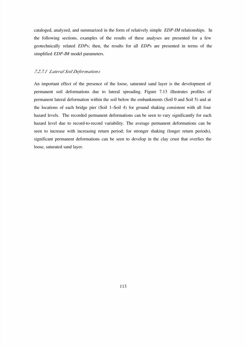
7/21/2019 PEER807 KRAMERArduino Shin
http://slidepdf.com/reader/full/peer807-kramerarduino-shin 126/198
113
cataloged, analyzed, and summarized in the form of relatively simple EDP-IM relationships. In
the following sections, examples of the results of these analyses are presented for a few
geotechnically related EDPs; then, the results for all EDPs are presented in terms of the
simplified EDP-IM model parameters.
7.2.7.1 Lateral Soil Deformations
An important effect of the presence of the loose, saturated sand layer is the development of
permanent soil deformations due to lateral spreading. Figure 7.13 illustrates profiles of
permanent lateral deformation within the soil below the embankments (Soil 0 and Soil 5) and at
the locations of each bridge pier (Soil 1–Soil 4) for ground shaking consistent with all four
hazard levels. The recorded permanent deformations can be seen to vary significantly for eachhazard level due to record-to-record variability. The average permanent deformations can be
seen to increase with increasing return period; for stronger shaking (longer return periods),
significant permanent deformations can be seen to develop in the clay crust that overlies the
loose, saturated sand layer.
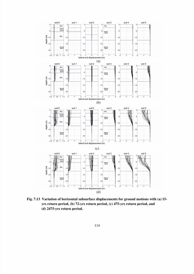
7/21/2019 PEER807 KRAMERArduino Shin
http://slidepdf.com/reader/full/peer807-kramerarduino-shin 127/198
114
(a)
(b)
(c)
(d)
Fig. 7.13 Variation of horizontal subsurface displacements for ground motions with (a) 15-
yrs return period, (b) 72-yrs return period, (c) 475-yrs return period, and
(d) 2475-yrs return period.
7/21/2019 PEER807 KRAMERArduino Shin
http://slidepdf.com/reader/full/peer807-kramerarduino-shin 128/198
115
Lateral spreading can also be seen to generally be greater below the right abutment (Soil
5) than the left abutment (Soil 0), thereby implying that damage to the bridge would be larger on
the right side than on the left. An evaluation of the drift demands on the bridge columns,
however, shows that the global interaction between the bridge, its foundations, and the soil
serves to shift the bridge deck to the left for some ground motions. As a result, the difference
between the displacements of the upper and lower ends of the bridge piers, as shown in Figure
7.14, are actually greater on the left side of the bridge (Pier 1) than on the right. (Pier 4). While
not observed for all motions, this aspect of potential system behavior represents a significant
potential mode of deformation that should be considered in design.
Fig. 7.14 Horizontal displacements at tops and bottoms of Piers 1 and 4. Note that absolute
displacement of Pier 4 (bottom) is larger than that of Pier 1, but difference between
top and bottom displacements is larger at Pier 1 than Pier 4.
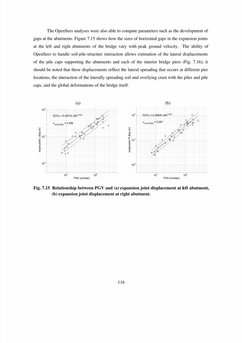
7/21/2019 PEER807 KRAMERArduino Shin
http://slidepdf.com/reader/full/peer807-kramerarduino-shin 129/198
116
The OpenSees analyses were also able to compute parameters such as the development of
gaps at the abutments. Figure 7.15 shows how the sizes of horizontal gaps in the expansion joints
at the left and right abutments of the bridge vary with peak ground velocity. The ability of
OpenSees to handle soil-pile-structure interaction allows estimation of the lateral displacements
of the pile caps supporting the abutments and each of the interior bridge piers (Fig. 7.16); it
should be noted that these displacements reflect the lateral spreading that occurs at different pier
locations, the interaction of the laterally spreading soil and overlying crust with the piles and pile
caps, and the global deformations of the bridge itself.
(a) (b)
Fig. 7.15 Relationship between PGV and (a) expansion joint displacement at left abutment,
(b) expansion joint displacement at right abutment.
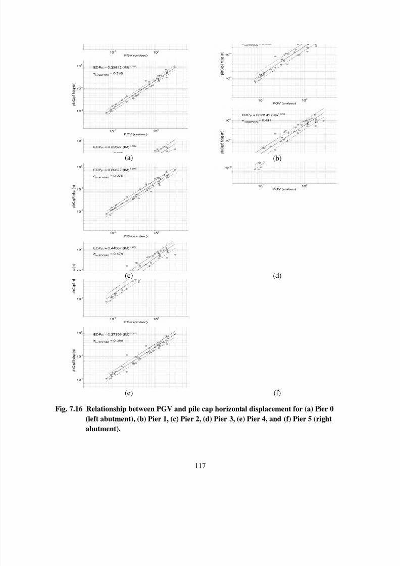
7/21/2019 PEER807 KRAMERArduino Shin
http://slidepdf.com/reader/full/peer807-kramerarduino-shin 130/198
117
(a) (b)
(c) (d)
(e) (f)
Fig. 7.16 Relationship between PGV and pile cap horizontal displacement for (a) Pier 0
(left abutment), (b) Pier 1, (c) Pier 2, (d) Pier 3, (e) Pier 4, and (f) Pier 5 (right
abutment).
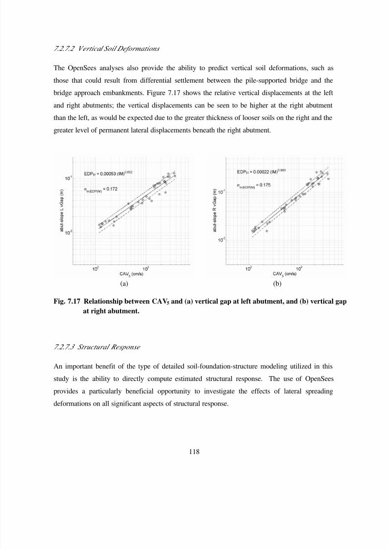
7/21/2019 PEER807 KRAMERArduino Shin
http://slidepdf.com/reader/full/peer807-kramerarduino-shin 131/198
118
7.2.7.2 Vertical Soil Deformations
The OpenSees analyses also provide the ability to predict vertical soil deformations, such as
those that could result from differential settlement between the pile-supported bridge and the
bridge approach embankments. Figure 7.17 shows the relative vertical displacements at the left
and right abutments; the vertical displacements can be seen to be higher at the right abutment
than the left, as would be expected due to the greater thickness of looser soils on the right and the
greater level of permanent lateral displacements beneath the right abutment.
(a) (b)
Fig. 7.17 Relationship between CAV5 and (a) vertical gap at left abutment, and (b) vertical gap
at right abutment.
7.2.7.3
Structural Response
An important benefit of the type of detailed soil-foundation-structure modeling utilized in this
study is the ability to directly compute estimated structural response. The use of OpenSees
provides a particularly beneficial opportunity to investigate the effects of lateral spreading
deformations on all significant aspects of structural response.
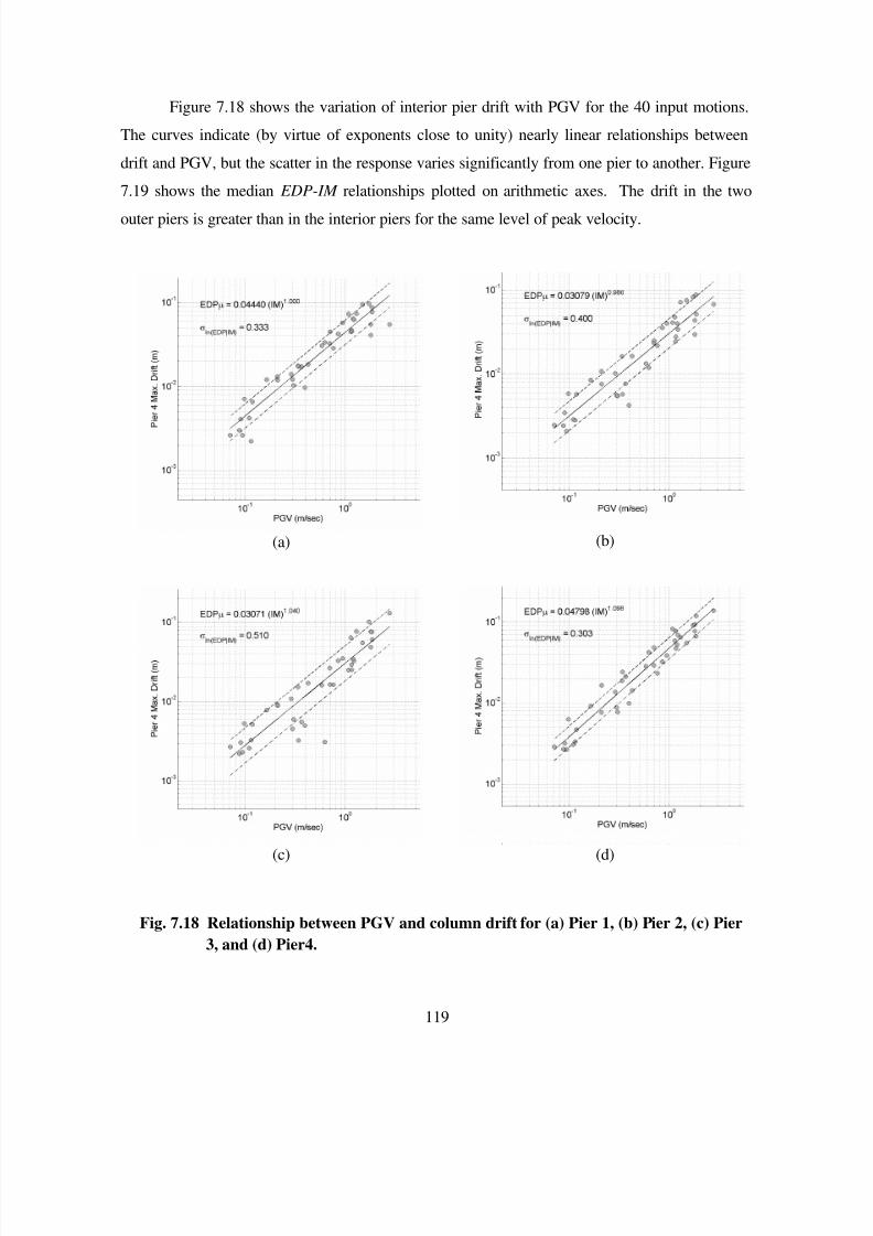
7/21/2019 PEER807 KRAMERArduino Shin
http://slidepdf.com/reader/full/peer807-kramerarduino-shin 132/198
119
Figure 7.18 shows the variation of interior pier drift with PGV for the 40 input motions.
The curves indicate (by virtue of exponents close to unity) nearly linear relationships between
drift and PGV, but the scatter in the response varies significantly from one pier to another. Figure
7.19 shows the median EDP-IM relationships plotted on arithmetic axes. The drift in the two
outer piers is greater than in the interior piers for the same level of peak velocity.
(a) (b)
(c) (d)
Fig. 7.18 Relationship between PGV and column drift for (a) Pier 1, (b) Pier 2, (c) Pier
3, and (d) Pier4.
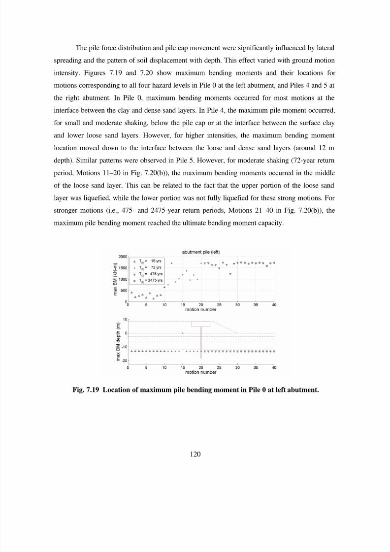
7/21/2019 PEER807 KRAMERArduino Shin
http://slidepdf.com/reader/full/peer807-kramerarduino-shin 133/198
120
The pile force distribution and pile cap movement were significantly influenced by lateral
spreading and the pattern of soil displacement with depth. This effect varied with ground motion
intensity. Figures 7.19 and 7.20 show maximum bending moments and their locations for
motions corresponding to all four hazard levels in Pile 0 at the left abutment, and Piles 4 and 5 at
the right abutment. In Pile 0, maximum bending moments occurred for most motions at the
interface between the clay and dense sand layers. In Pile 4, the maximum pile moment occurred,
for small and moderate shaking, below the pile cap or at the interface between the surface clay
and lower loose sand layers. However, for higher intensities, the maximum bending moment
location moved down to the interface between the loose and dense sand layers (around 12 m
depth). Similar patterns were observed in Pile 5. However, for moderate shaking (72-year return
period, Motions 11–20 in Fig. 7.20(b)), the maximum bending moments occurred in the middle
of the loose sand layer. This can be related to the fact that the upper portion of the loose sand
layer was liquefied, while the lower portion was not fully liquefied for these strong motions. For
stronger motions (i.e., 475- and 2475-year return periods, Motions 21–40 in Fig. 7.20(b)), the
maximum pile bending moment reached the ultimate bending moment capacity.
Fig. 7.19 Location of maximum pile bending moment in Pile 0 at left abutment.
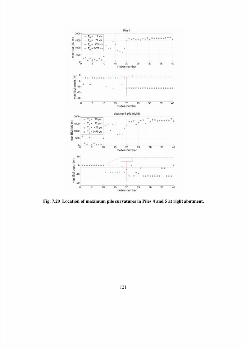
7/21/2019 PEER807 KRAMERArduino Shin
http://slidepdf.com/reader/full/peer807-kramerarduino-shin 134/198
121
Fig. 7.20 Location of maximum pile curvatures in Piles 4 and 5 at right abutment.
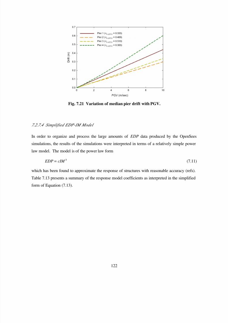
7/21/2019 PEER807 KRAMERArduino Shin
http://slidepdf.com/reader/full/peer807-kramerarduino-shin 135/198
122
Fig. 7.21 Variation of median pier drift with PGV.
7.2.7.4 Simplified EDP-IM Model
In order to organize and process the large amounts of EDP data produced by the OpenSees
simulations, the results of the simulations were interpreted in terms of a relatively simple power
law model. The model is of the power law form
b
cIM EDP = (7.11)
which has been found to approximate the response of structures with reasonable accuracy (refs).
Table 7.13 presents a summary of the response model coefficients as interpreted in the simplified
form of Equation (7.13).
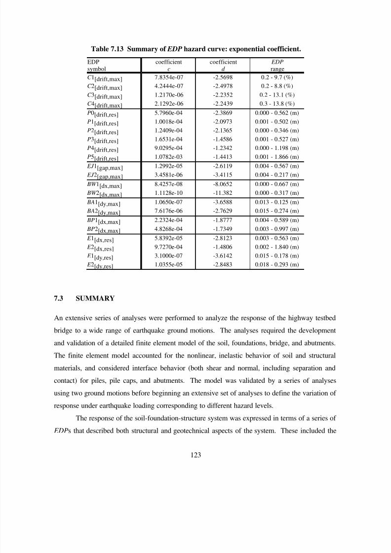
7/21/2019 PEER807 KRAMERArduino Shin
http://slidepdf.com/reader/full/peer807-kramerarduino-shin 136/198
123
Table 7.13 Summary of EDP hazard curve: exponential coefficient.
EDPsymbol
coefficientc
coefficientd
EDP range
C 1[drift,max] 7.8354e-07 -2.5698 0.2 - 9.7 (%)
C 2[drift,max] 4.2444e-07 -2.4978 0.2 - 8.8 (%)
C 3[drift,max] 1.2170e-06 -2.2352 0.2 - 13.1 (%)
C 4[drift,max] 2.1292e-06 -2.2439 0.3 - 13.8 (%)
P0[drift,res] 5.7960e-04 -2.3869 0.000 - 0.562 (m)
P1[drift,res] 1.0018e-04 -2.0973 0.001 - 0.502 (m)
P2[drift,res] 1.2409e-04 -2.1365 0.000 - 0.346 (m)
P3[drift,res] 1.6531e-04 -1.4586 0.001 - 0.527 (m)
P4[drift,res] 9.0295e-04 -1.2342 0.000 - 1.198 (m)
P5[drift,res] 1.0782e-03 -1.4413 0.001 - 1.866 (m)
EJ 1[gap,max] 1.2992e-05 -2.6119 0.004 - 0.567 (m)
EJ 2[gap,max] 3.4581e-06 -3.4115 0.004 - 0.217 (m)
BW 1[dx,max] 8.4257e-08 -8.0652 0.000 - 0.667 (m) BW 2[dx,max] 1.1128e-10 -11.382 0.000 - 0.317 (m)
BA1[dy,max] 1.0650e-07 -3.6588 0.013 - 0.125 (m)
BA2[dy,max] 7.6176e-06 -2.7629 0.015 - 0.274 (m)
BP1[dx,max] 2.2324e-04 -1.8777 0.004 - 0.589 (m)
BP2[dx,max] 4.8268e-04 -1.7349 0.003 - 0.997 (m)
E 1[dx,res] 5.8392e-05 -2.8123 0.003 - 0.563 (m)
E 2[dx,res] 9.7270e-04 -1.4806 0.002 - 1.840 (m)
E 1[dy,res] 3.1000e-07 -3.6142 0.015 - 0.178 (m)
E 2[dy,res] 1.0355e-05 -2.8483 0.018 - 0.293 (m)
7.3 SUMMARY
An extensive series of analyses were performed to analyze the response of the highway testbed
bridge to a wide range of earthquake ground motions. The analyses required the development
and validation of a detailed finite element model of the soil, foundations, bridge, and abutments.
The finite element model accounted for the nonlinear, inelastic behavior of soil and structural
materials, and considered interface behavior (both shear and normal, including separation andcontact) for piles, pile caps, and abutments. The model was validated by a series of analyses
using two ground motions before beginning an extensive set of analyses to define the variation of
response under earthquake loading corresponding to different hazard levels.
The response of the soil-foundation-structure system was expressed in terms of a series of
EDPs that described both structural and geotechnical aspects of the system. These included the

7/21/2019 PEER807 KRAMERArduino Shin
http://slidepdf.com/reader/full/peer807-kramerarduino-shin 137/198
124
drift of each column, displacement of each pile cap, displacement of each expansion joint,
displacement of each abutment backwall, vertical offset at each abutment due to approach
embankment settlement, displacement of each bearing pad, and the vertical and horizontal
movement of each approach embankment.
The responses to 10 ground motions at each of four hazard levels was found to be
reasonably represented by a simple power law relationship between EDP and IM . The relative
efficiencies of a series of candidate IM s were investigated; different IM s were observed to be
most efficient for different EDPs, but PGV was selected as the single most useful IM for the
purpose of response, damage, and loss estimation. Power law relationships between PGV and all
of the selected EDPs were established; the fragility curves based on these EDP- IM
relationships were used for subsequent estimation of damage and loss.
7/21/2019 PEER807 KRAMERArduino Shin
http://slidepdf.com/reader/full/peer807-kramerarduino-shin 138/198
8 Foundation Damage and Loss
8.1 INTRODUCTION
The bridge response computed using OpenSees analyses and described in the preceding chapter
provides a basis for estimating the recurrence rate of different levels of physical damage to the
bridge. Such estimates of physical damage can provide the basis for subsequent loss estimation
using the PEER PBEE framework described in Chapter 2.
In order to produce loss ( DV ) estimates that could be directly compared with the loss
estimates produced by Mackie and Stojadinović (2007b) for the fixed-base bridge model, the
loss model developed by Mackie and Stojadinović was used. The initial version of this loss
model did not produce explicit damage estimates for all of the performance groups for which
EDPs were computed. In order to investigate the effects of liquefaction-induced lateral
spreading on foundation performance, damage and loss models were developed for the pile-
supported bridge foundations. This chapter describes these models and the levels of physical
foundation damage and loss they predicted. A more complete loss model for the entire structure,
including the foundations, is described in Chapter 9.
8.2 DAMAGE AND LOSS PROBABILITY MATRIX APPROACH
In the absence of data on physical damage and loss in the early stages of the project, a discrete
damage and loss probability estimation approach was developed. This approach involved the
development of damage and loss probability matrices for the pile-supported bridge foundations.
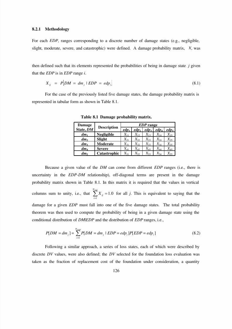
7/21/2019 PEER807 KRAMERArduino Shin
http://slidepdf.com/reader/full/peer807-kramerarduino-shin 139/198
126
8.2.1 Methodology
For each EDP, ranges corresponding to a discrete number of damage states (e.g., negligible,
slight, moderate, severe, and catastrophic) were defined. A damage probability matrix, X , was
then defined such that its elements represented the probabilities of being in damage state j given
that the EDP is in EDP range i.
i jij edp| EDPdm DMP X === (8.1)
For the case of the previously listed five damage states, the damage probability matrix is
represented in tabular form as shown in Table 8.1.
Table 8.1 Damage probability matrix.
EDP rangeDamage
State, DM Description
edp1 edp2 edp3 edp4 edp5
dm1 Negligible X 11 X 12 X 13 X 14 X 15
dm2 Slight X 21 X 22 X 23 X 24 X 25
dm3 Moderate X 31 X 32 X 33 X 34 X 35
dm4 Severe X 41 X 42 X 43 X 44 X 45
dm5 Catastrophic X 51 X 52 X 53 X 54 X 55
Because a given value of the DM can come from different EDP ranges (i.e., there is
uncertainty in the EDP-DM relationship), off-diagonal terms are present in the damage
probability matrix shown in Table 8.1. In this matrix it is required that the values in vertical
columns sum to unity, i.e., that ∑=
= DM N
i
ij X 1
0.1 for all j. This is equivalent to saying that the
damage for a given EDP must fall into one of the five damage states. The total probability
theorem was then used to compute the probability of being in a given damage state using the
conditional distribution of DM | EDP and the distribution of EDP ranges, i.e.,
∑=
===== EDP N
i
ii j j edp EDPPedp EDPdm DM Pdm DM P1
][]|[][ (8.2)
Following a similar approach, a series of loss states, each of which were described by
discrete DV values, were also defined; the DV selected for the foundation loss evaluation was
taken as the fraction of replacement cost of the foundation under consideration, a quantity
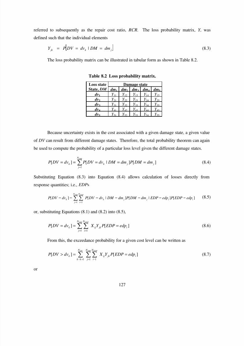
7/21/2019 PEER807 KRAMERArduino Shin
http://slidepdf.com/reader/full/peer807-kramerarduino-shin 140/198
127
referred to subsequently as the repair cost ratio, RCR. The loss probability matrix, Y, was
defined such that the individual elements
jk jk dm| DMdv DVP Y === (8.3)
The loss probability matrix can be illustrated in tabular form as shown in Table 8.2.
Table 8.2 Loss probability matrix.
Damage stateLoss stateState, DM dm1 dm2 dm3 dm4 dm5
dv1 Y 11 Y 12 Y 13 Y 14 Y 15
dv2 Y 21 Y 22 Y 23 Y 24 Y 25
dv3 Y 31 Y 32 Y 33 Y 34 Y 35
dv4 Y 41 Y 42 Y 43 Y 44 Y 45
dv5 Y 51 Y 52 Y 53 Y 54 Y 55
Because uncertainty exists in the cost associated with a given damage state, a given value
of DV can result from different damage states. Therefore, the total probability theorem can again
be used to compute the probability of a particular loss level given the different damage states.
∑=
===== DM N
j
j jk k dm DM Pdm DM dv DV Pdv DV P1
][]|[][ (8.4)
Substituting Equation (8.3) into Equation (8.4) allows calculation of losses directly from
response quantities; i.e., EDPs
∑∑= =
======= DM EDP N
j
ii j jk
N
i
k edp EDPPedp EDPdm DM Pdm DM dv DV Pdv DV P1 1
][]|[]|[][ (8.5)
or, substituting Equations (8.1) and (8.2) into (8.5),
∑∑= =
=== DM EDP N
j
i jk ij
N
i
k edp EDPPY X dv DV P
1 1
][][ (8.6)
From this, the exceedance probability for a given cost level can be written as
∑∑∑= =+=
==> DM EDP DV N
j
i jk ij
N
i
N
k k
k edp EDPPY X dv DV P1 11
][][ (8.7)
or
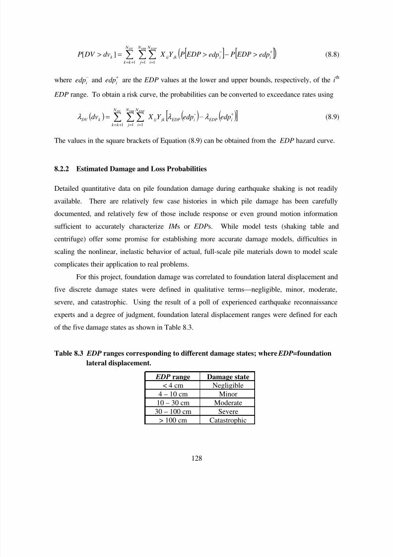
7/21/2019 PEER807 KRAMERArduino Shin
http://slidepdf.com/reader/full/peer807-kramerarduino-shin 141/198
128
[ ] [ ]( )∑∑∑=
+−
=+=
>−>=> DM EDP DV N
j
ii jk ij
N
i
N
k k
k edp EDPPedp EDPPY X dv DV P1 11
][ (8.8)
where edpi
− and edp
i
+ are the EDP values at the lower and upper bounds, respectively, of the i
th
EDP range. To obtain a risk curve, the probabilities can be converted to exceedance rates using
( ) ( ) ( )[ ]∑∑∑=
+−
=+=
−= DM EDP DV N
j
i EDPi EDP jk ij
N
i
N
k k
k DV edpedpY X dv1 11
λ λ λ (8.9)
The values in the square brackets of Equation (8.9) can be obtained from the EDP hazard curve.
8.2.2 Estimated Damage and Loss Probabilities
Detailed quantitative data on pile foundation damage during earthquake shaking is not readily
available. There are relatively few case histories in which pile damage has been carefully
documented, and relatively few of those include response or even ground motion information
sufficient to accurately characterize IM s or EDPs. While model tests (shaking table and
centrifuge) offer some promise for establishing more accurate damage models, difficulties in
scaling the nonlinear, inelastic behavior of actual, full-scale pile materials down to model scale
complicates their application to real problems.
For this project, foundation damage was correlated to foundation lateral displacement andfive discrete damage states were defined in qualitative terms—negligible, minor, moderate,
severe, and catastrophic. Using the result of a poll of experienced earthquake reconnaissance
experts and a degree of judgment, foundation lateral displacement ranges were defined for each
of the five damage states as shown in Table 8.3.
Table 8.3 EDP ranges corresponding to different damage states; where EDP=foundation
lateral displacement.
EDP range Damage state
< 4 cm Negligible
4 – 10 cm Minor
10 – 30 cm Moderate
30 – 100 cm Severe
> 100 cm Catastrophic
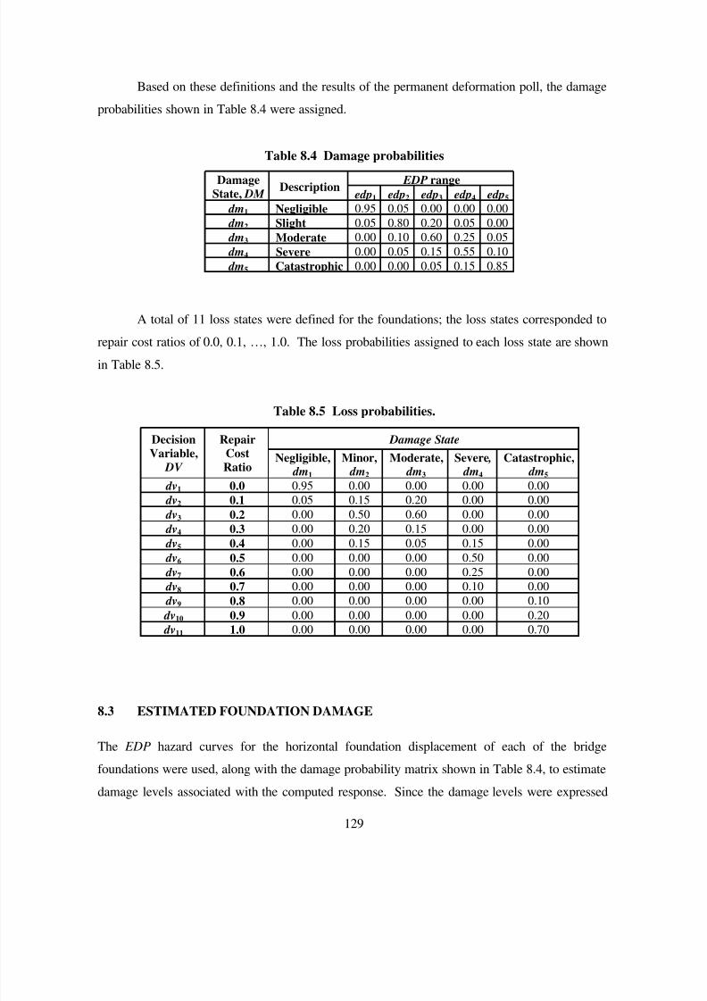
7/21/2019 PEER807 KRAMERArduino Shin
http://slidepdf.com/reader/full/peer807-kramerarduino-shin 142/198
129
Based on these definitions and the results of the permanent deformation poll, the damage
probabilities shown in Table 8.4 were assigned.
Table 8.4 Damage probabilities
EDP rangeDamage
State, DM Description
edp1 edp2 edp3 edp4 edp5
dm1 Negligible 0.95 0.05 0.00 0.00 0.00
dm2 Slight 0.05 0.80 0.20 0.05 0.00
dm3 Moderate 0.00 0.10 0.60 0.25 0.05
dm4 Severe 0.00 0.05 0.15 0.55 0.10
dm5 Catastrophic 0.00 0.00 0.05 0.15 0.85
A total of 11 loss states were defined for the foundations; the loss states corresponded to
repair cost ratios of 0.0, 0.1, …, 1.0. The loss probabilities assigned to each loss state are shown
in Table 8.5.
Table 8.5 Loss probabilities.
Damage State Decision
Variable,
DV
Repair
Cost
RatioNegligible,
dm1
Minor, dm2
Moderate, dm3
Severe ,
dm4
Catastrophic, dm5
dv1 0.0 0.95 0.00 0.00 0.00 0.00
dv2 0.1 0.05 0.15 0.20 0.00 0.00 dv3 0.2 0.00 0.50 0.60 0.00 0.00
dv4 0.3 0.00 0.20 0.15 0.00 0.00
dv5 0.4 0.00 0.15 0.05 0.15 0.00
dv6 0.5 0.00 0.00 0.00 0.50 0.00
dv7 0.6 0.00 0.00 0.00 0.25 0.00
dv8 0.7 0.00 0.00 0.00 0.10 0.00
dv9 0.8 0.00 0.00 0.00 0.00 0.10
dv10 0.9 0.00 0.00 0.00 0.00 0.20
dv11 1.0 0.00 0.00 0.00 0.00 0.70
8.3 ESTIMATED FOUNDATION DAMAGE
The EDP hazard curves for the horizontal foundation displacement of each of the bridge
foundations were used, along with the damage probability matrix shown in Table 8.4, to estimate
damage levels associated with the computed response. Since the damage levels were expressed
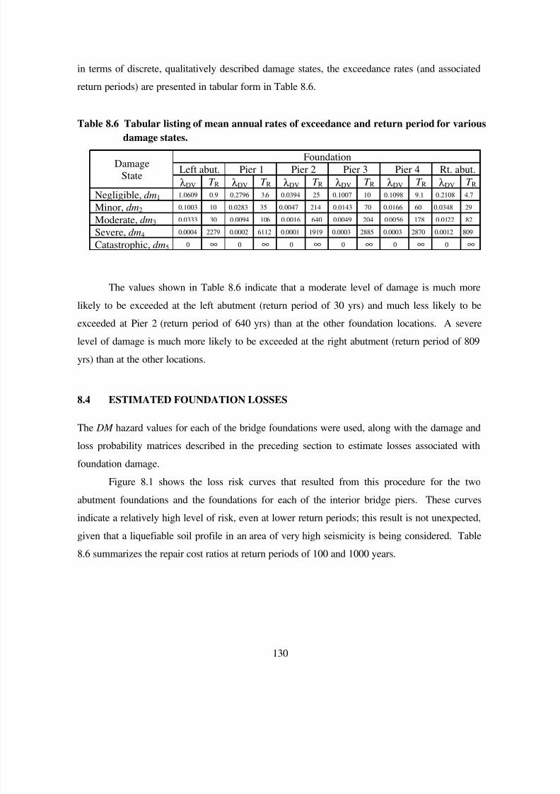
7/21/2019 PEER807 KRAMERArduino Shin
http://slidepdf.com/reader/full/peer807-kramerarduino-shin 143/198
130
in terms of discrete, qualitatively described damage states, the exceedance rates (and associated
return periods) are presented in tabular form in Table 8.6.
Table 8.6 Tabular listing of mean annual rates of exceedance and return period for various
damage states.
Foundation
Left abut. Pier 1 Pier 2 Pier 3 Pier 4 Rt. abut.Damage
Stateλ DV T R λ DV T R λ DV T R λ DV T R λ DV T R λ DV T R
Negligible, dm1 1.0609 0.9 0.2796 3.6 0.0394 25 0.1007 10 0.1098 9.1 0.2108 4.7
Minor, dm2 0.1003 10 0.0283 35 0.0047 214 0.0143 70 0.0166 60 0.0348 29
Moderate, dm3 0.0333 30 0.0094 106 0.0016 640 0.0049 204 0.0056 178 0.0122 82
Severe, dm4 0.0004 2279 0.0002 6112 0.0001 1919 0.0003 2885 0.0003 2870 0.0012 809
Catastrophic, dm5 0 ∞ 0 ∞ 0 ∞ 0 ∞ 0 ∞ 0 ∞
The values shown in Table 8.6 indicate that a moderate level of damage is much more
likely to be exceeded at the left abutment (return period of 30 yrs) and much less likely to be
exceeded at Pier 2 (return period of 640 yrs) than at the other foundation locations. A severe
level of damage is much more likely to be exceeded at the right abutment (return period of 809
yrs) than at the other locations.
8.4 ESTIMATED FOUNDATION LOSSES
The DM hazard values for each of the bridge foundations were used, along with the damage and
loss probability matrices described in the preceding section to estimate losses associated with
foundation damage.
Figure 8.1 shows the loss risk curves that resulted from this procedure for the two
abutment foundations and the foundations for each of the interior bridge piers. These curves
indicate a relatively high level of risk, even at lower return periods; this result is not unexpected,
given that a liquefiable soil profile in an area of very high seismicity is being considered. Table
8.6 summarizes the repair cost ratios at return periods of 100 and 1000 years.

7/21/2019 PEER807 KRAMERArduino Shin
http://slidepdf.com/reader/full/peer807-kramerarduino-shin 144/198
131
Table 8.7 Estimated loss levels.
Foundation 100-yr RCR 1,000-yr RCR
Left abutment 0.62 0.77
Pier 1 0.46 0.71Pier 2 0.24 0.53
Pier 3 0.35 0.67
Pier 4 0.37 0.69
Right abutment 0.52 0.93
As the curves of Figure 8.1 and tabulated values in Table 8.5 indicate, the estimated
foundation losses are highest for the left abutment at the 100-years hazard level, and highest at
the right abutment for the 1000-years hazard level. Pier 2, which is subjected to the lowest levelsof lateral spreading-induced soil deformations, has significantly lower expected losses than do
the other foundations at both hazard levels.
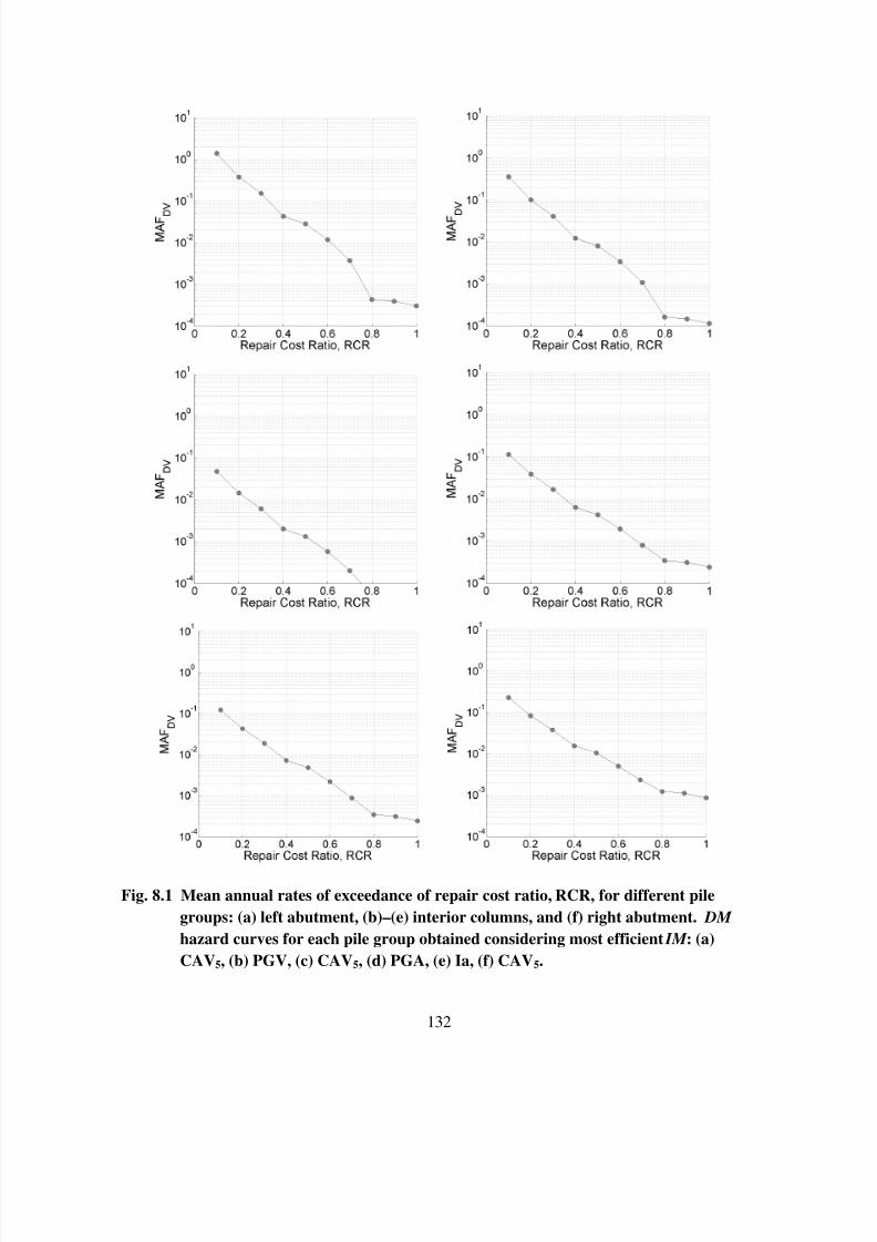
7/21/2019 PEER807 KRAMERArduino Shin
http://slidepdf.com/reader/full/peer807-kramerarduino-shin 145/198
132
Fig. 8.1 Mean annual rates of exceedance of repair cost ratio, RCR, for different pile
groups: (a) left abutment, (b)–(e) interior columns, and (f) right abutment. DM
hazard curves for each pile group obtained considering most efficient IM : (a)
CAV5, (b) PGV, (c) CAV5, (d) PGA, (e) Ia, (f) CAV5.

7/21/2019 PEER807 KRAMERArduino Shin
http://slidepdf.com/reader/full/peer807-kramerarduino-shin 146/198
133
8.5 SUMMARY
Using a procedure in which damage and loss probability matrices were developed for a small
number of discrete damage states and a larger number of loss levels, the EDP hazard curves for
each of the bridge foundations were used to estimate damage hazards and produce loss hazard
curves. The relatively simple and monotonic relationship between damage and response and
between loss and damage led to generally predictable results when interpreted in a relative
sense—the foundations that experienced the highest levels of predicted response were observed
to have the highest expected loss levels. However, the inclusion of uncertainty in damage and
loss predictions allows quantitative estimation of the mean annual rates of exceedance of the
different damage and loss levels.
7/21/2019 PEER807 KRAMERArduino Shin
http://slidepdf.com/reader/full/peer807-kramerarduino-shin 147/198
135
9 Bridge Damage and Loss
9.1 INTRODUCTION
The bridge response computed using OpenSees analyses and described in Chapter 7 also
provides a basis for estimating the recurrence rate of different levels of physical damage and loss
for the entire bridge system. In order to facilitate comparisons of damage and loss for the testbed
highway bridge considered in this research project with that of the same bridge under fixed-base
conditions, the damage and loss model developed by Mackie and Stojadinović (2006) was
modified to account for geotechnical/foundation-related damage and loss and then used to
estimate total bridge damage and loss.
This chapter presents the results of a series of bridge damage and loss analyses, and
examines the sensitivity of losses to various assumptions in the modeling of damage and loss. It
also examines the question of how loss estimates would be affected by a lack of EDP
information, as could be the case if a simpler response model was used.
9.2 DAMAGE MODELS
In order to estimate bridge damage, the main components of the bridge were divided into 21
performance groups. The most efficient EDPs were identified for each of the performance
groups; the performance groups and EDPs are listed in Table 9.1. Multiple components were
considered in some of the performance groups (four columns, for example, in the Column
performance group). The following descriptions are based on Mackie et al. (2006).
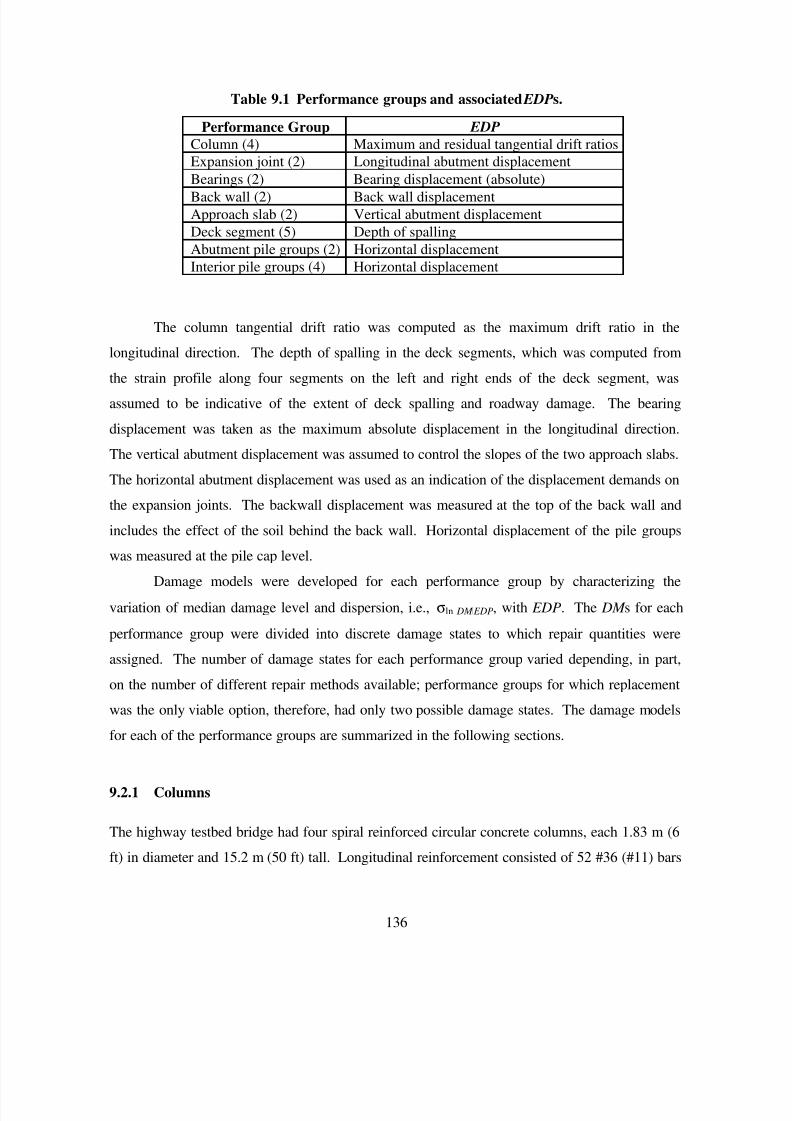
7/21/2019 PEER807 KRAMERArduino Shin
http://slidepdf.com/reader/full/peer807-kramerarduino-shin 148/198
136
Table 9.1 Performance groups and associated EDPs.
Performance Group EDP
Column (4) Maximum and residual tangential drift ratiosExpansion joint (2) Longitudinal abutment displacement
Bearings (2) Bearing displacement (absolute)
Back wall (2) Back wall displacement
Approach slab (2) Vertical abutment displacement
Deck segment (5) Depth of spalling
Abutment pile groups (2) Horizontal displacement
Interior pile groups (4) Horizontal displacement
The column tangential drift ratio was computed as the maximum drift ratio in the
longitudinal direction. The depth of spalling in the deck segments, which was computed from
the strain profile along four segments on the left and right ends of the deck segment, was
assumed to be indicative of the extent of deck spalling and roadway damage. The bearing
displacement was taken as the maximum absolute displacement in the longitudinal direction.
The vertical abutment displacement was assumed to control the slopes of the two approach slabs.
The horizontal abutment displacement was used as an indication of the displacement demands on
the expansion joints. The backwall displacement was measured at the top of the back wall and
includes the effect of the soil behind the back wall. Horizontal displacement of the pile groups
was measured at the pile cap level.Damage models were developed for each performance group by characterizing the
variation of median damage level and dispersion, i.e., σln DM | EDP, with EDP. The DM s for each
performance group were divided into discrete damage states to which repair quantities were
assigned. The number of damage states for each performance group varied depending, in part,
on the number of different repair methods available; performance groups for which replacement
was the only viable option, therefore, had only two possible damage states. The damage models
for each of the performance groups are summarized in the following sections.
9.2.1 Columns
The highway testbed bridge had four spiral reinforced circular concrete columns, each 1.83 m (6
ft) in diameter and 15.2 m (50 ft) tall. Longitudinal reinforcement consisted of 52 #36 (#11) bars
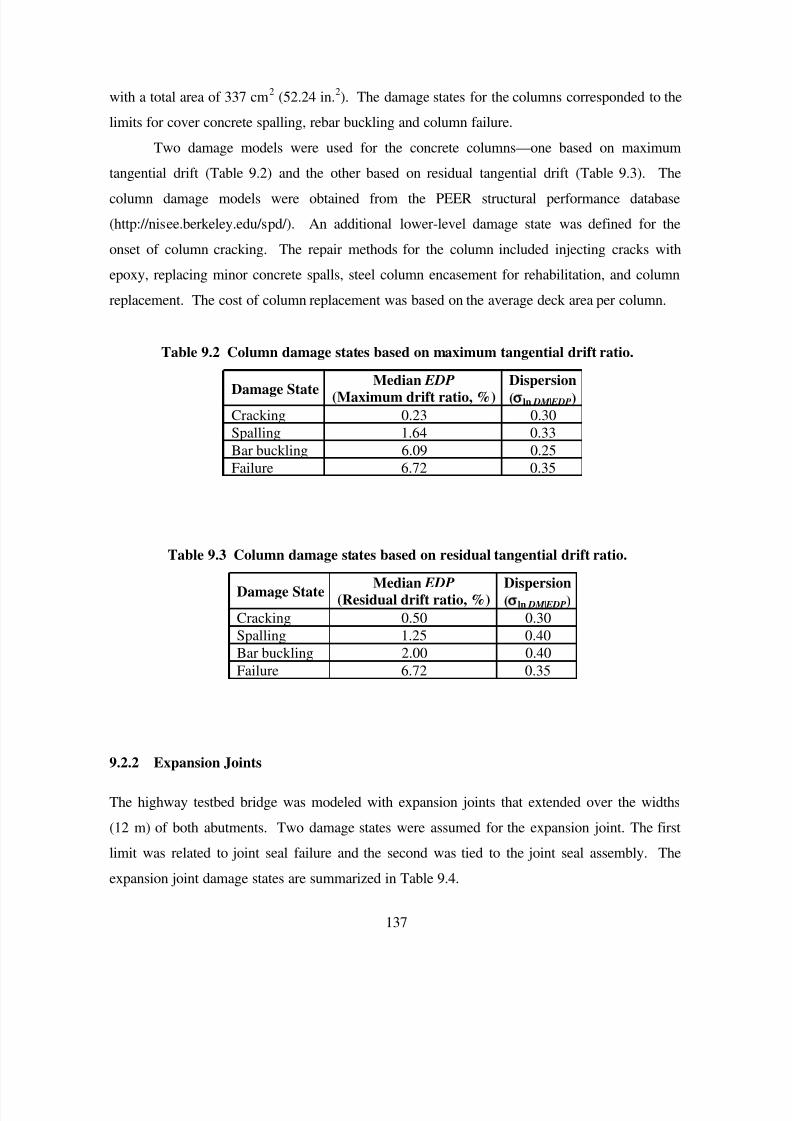
7/21/2019 PEER807 KRAMERArduino Shin
http://slidepdf.com/reader/full/peer807-kramerarduino-shin 149/198
137
with a total area of 337 cm2 (52.24 in.
2). The damage states for the columns corresponded to the
limits for cover concrete spalling, rebar buckling and column failure.
Two damage models were used for the concrete columns—one based on maximum
tangential drift (Table 9.2) and the other based on residual tangential drift (Table 9.3). The
column damage models were obtained from the PEER structural performance database
(http://nisee.berkeley.edu/spd/). An additional lower-level damage state was defined for the
onset of column cracking. The repair methods for the column included injecting cracks with
epoxy, replacing minor concrete spalls, steel column encasement for rehabilitation, and column
replacement. The cost of column replacement was based on the average deck area per column.
Table 9.2 Column damage states based on maximum tangential drift ratio.
Damage StateMedian EDP
(Maximum drift ratio, %)
Dispersion
( ln DM | EDP)
Cracking 0.23 0.30
Spalling 1.64 0.33
Bar buckling 6.09 0.25
Failure 6.72 0.35
Table 9.3 Column damage states based on residual tangential drift ratio.
Damage StateMedian EDP
(Residual drift ratio, %)
Dispersion
( ln DM | EDP)
Cracking 0.50 0.30
Spalling 1.25 0.40
Bar buckling 2.00 0.40
Failure 6.72 0.35
9.2.2 Expansion Joints
The highway testbed bridge was modeled with expansion joints that extended over the widths
(12 m) of both abutments. Two damage states were assumed for the expansion joint. The first
limit was related to joint seal failure and the second was tied to the joint seal assembly. The
expansion joint damage states are summarized in Table 9.4.
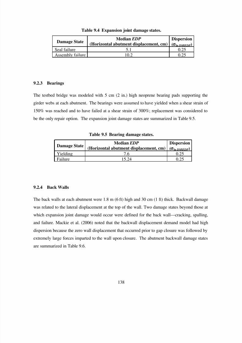
7/21/2019 PEER807 KRAMERArduino Shin
http://slidepdf.com/reader/full/peer807-kramerarduino-shin 150/198
138
Table 9.4 Expansion joint damage states.
Damage StateMedian EDP
(Horizontal abutment displacement, cm)
Dispersion
( ln DM | EDP)
Seal failure 5.1 0.25
Assembly failure 10.2 0.25
9.2.3 Bearings
The testbed bridge was modeled with 5 cm (2 in.) high neoprene bearing pads supporting the
girder webs at each abutment. The bearings were assumed to have yielded when a shear strain of
150% was reached and to have failed at a shear strain of 300%; replacement was considered to
be the only repair option. The expansion joint damage states are summarized in Table 9.5.
Table 9.5 Bearing damage states.
Damage StateMedian EDP
(Horizontal abutment displacement, cm)
Dispersion
( ln DM | EDP)
Yielding 7.6 0.25
Failure 15.24 0.25
9.2.4 Back Walls
The back walls at each abutment were 1.8 m (6 ft) high and 30 cm (1 ft) thick. Backwall damage
was related to the lateral displacement at the top of the wall. Two damage states beyond those at
which expansion joint damage would occur were defined for the back wall—cracking, spalling,
and failure. Mackie et al. (2006) noted that the backwall displacement demand model had high
dispersion because the zero wall displacement that occurred prior to gap closure was followed by
extremely large forces imparted to the wall upon closure. The abutment backwall damage states
are summarized in Table 9.6.
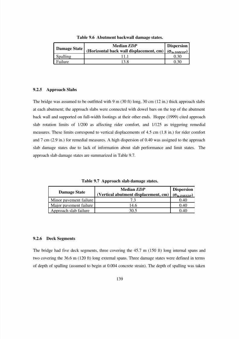
7/21/2019 PEER807 KRAMERArduino Shin
http://slidepdf.com/reader/full/peer807-kramerarduino-shin 151/198
139
Table 9.6 Abutment backwall damage states.
Damage StateMedian EDP
(Horizontal back wall displacement, cm)
Dispersion
( ln DM | EDP)
Spalling 11.1 0.30Failure 13.8 0.30
9.2.5 Approach Slabs
The bridge was assumed to be outfitted with 9 m (30 ft) long, 30 cm (12 in.) thick approach slabs
at each abutment; the approach slabs were connected with dowel bars on the top of the abutment
back wall and supported on full-width footings at their other ends. Hoppe (1999) cited approach
slab rotation limits of 1/200 as affecting rider comfort, and 1/125 as triggering remedial
measures. These limits correspond to vertical displacements of 4.5 cm (1.8 in.) for rider comfort
and 7 cm (2.9 in.) for remedial measures. A high dispersion of 0.40 was assigned to the approach
slab damage states due to lack of information about slab performance and limit states. The
approach slab damage states are summarized in Table 9.7.
Table 9.7 Approach slab damage states.
Damage StateMedian EDP
(Vertical abutment displacement, cm)
Dispersion
( ln DM | EDP)
Minor pavement failure 7.3 0.40
Major pavement failure 14.6 0.40
Approach slab failure 30.5 0.40
9.2.6 Deck Segments
The bridge had five deck segments, three covering the 45.7 m (150 ft) long internal spans and
two covering the 36.6 m (120 ft) long external spans. Three damage states were defined in terms
of depth of spalling (assumed to begin at 0.004 concrete strain). The depth of spalling was taken
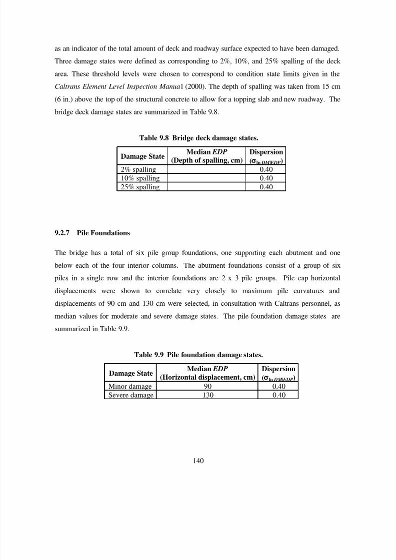
7/21/2019 PEER807 KRAMERArduino Shin
http://slidepdf.com/reader/full/peer807-kramerarduino-shin 152/198
140
as an indicator of the total amount of deck and roadway surface expected to have been damaged.
Three damage states were defined as corresponding to 2%, 10%, and 25% spalling of the deck
area. These threshold levels were chosen to correspond to condition state limits given in the
Caltrans Element Level Inspection Manual (2000). The depth of spalling was taken from 15 cm
(6 in.) above the top of the structural concrete to allow for a topping slab and new roadway. The
bridge deck damage states are summarized in Table 9.8.
Table 9.8 Bridge deck damage states.
Damage StateMedian EDP
(Depth of spalling, cm)
Dispersion
( ln DM | EDP)
2% spalling 0.40
10% spalling 0.40
25% spalling 0.40
9.2.7 Pile Foundations
The bridge has a total of six pile group foundations, one supporting each abutment and one
below each of the four interior columns. The abutment foundations consist of a group of six
piles in a single row and the interior foundations are 2 x 3 pile groups. Pile cap horizontaldisplacements were shown to correlate very closely to maximum pile curvatures and
displacements of 90 cm and 130 cm were selected, in consultation with Caltrans personnel, as
median values for moderate and severe damage states. The pile foundation damage states are
summarized in Table 9.9.
Table 9.9 Pile foundation damage states.
Damage State
Median EDP
(Horizontal displacement, cm)
Dispersion
( ln DM | EDP)
Minor damage 90 0.40
Severe damage 130 0.40
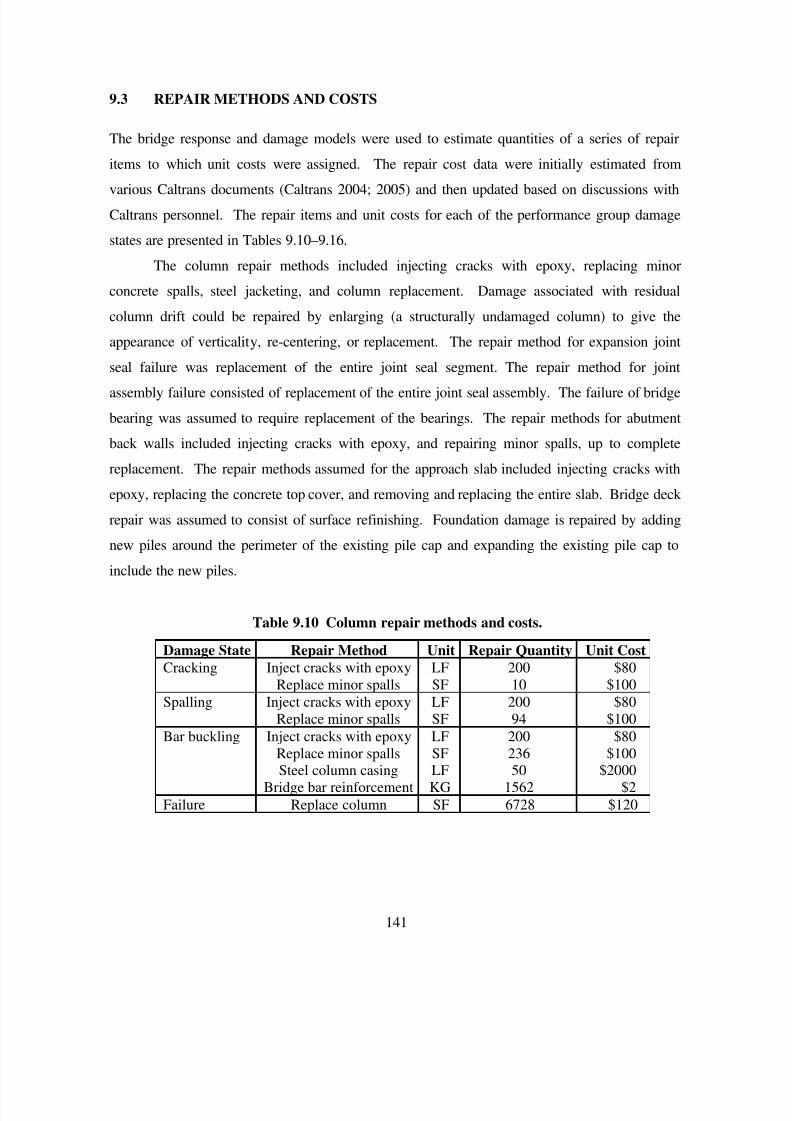
7/21/2019 PEER807 KRAMERArduino Shin
http://slidepdf.com/reader/full/peer807-kramerarduino-shin 153/198
141
9.3 REPAIR METHODS AND COSTS
The bridge response and damage models were used to estimate quantities of a series of repair
items to which unit costs were assigned. The repair cost data were initially estimated from
various Caltrans documents (Caltrans 2004; 2005) and then updated based on discussions with
Caltrans personnel. The repair items and unit costs for each of the performance group damage
states are presented in Tables 9.10–9.16.
The column repair methods included injecting cracks with epoxy, replacing minor
concrete spalls, steel jacketing, and column replacement. Damage associated with residual
column drift could be repaired by enlarging (a structurally undamaged column) to give the
appearance of verticality, re-centering, or replacement. The repair method for expansion joint
seal failure was replacement of the entire joint seal segment. The repair method for jointassembly failure consisted of replacement of the entire joint seal assembly. The failure of bridge
bearing was assumed to require replacement of the bearings. The repair methods for abutment
back walls included injecting cracks with epoxy, and repairing minor spalls, up to complete
replacement. The repair methods assumed for the approach slab included injecting cracks with
epoxy, replacing the concrete top cover, and removing and replacing the entire slab. Bridge deck
repair was assumed to consist of surface refinishing. Foundation damage is repaired by adding
new piles around the perimeter of the existing pile cap and expanding the existing pile cap to
include the new piles.
Table 9.10 Column repair methods and costs.
Damage State Repair Method Unit Repair Quantity Unit Cost
Cracking Inject cracks with epoxyReplace minor spalls
LFSF
20010
$80$100
Spalling Inject cracks with epoxyReplace minor spalls
LFSF
20094
$80$100
Bar buckling Inject cracks with epoxy
Replace minor spallsSteel column casing
Bridge bar reinforcement
LF
SFLFKG
200
23650
1562
$80
$100$2000
$2
Failure Replace column SF 6728 $120
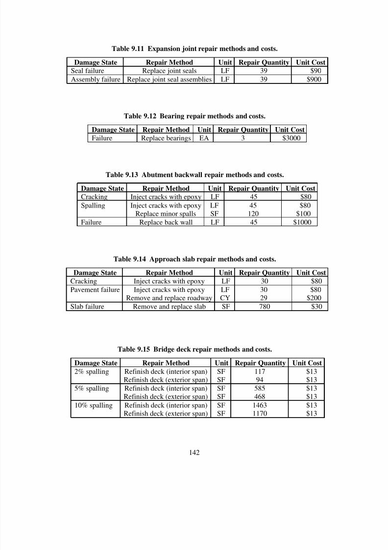
7/21/2019 PEER807 KRAMERArduino Shin
http://slidepdf.com/reader/full/peer807-kramerarduino-shin 154/198
142
Table 9.11 Expansion joint repair methods and costs.
Damage State Repair Method Unit Repair Quantity Unit Cost
Seal failure Replace joint seals LF 39 $90
Assembly failure Replace joint seal assemblies LF 39 $900
Table 9.12 Bearing repair methods and costs.
Damage State Repair Method Unit Repair Quantity Unit Cost
Failure Replace bearings EA 3 $3000
Table 9.13 Abutment backwall repair methods and costs.
Damage State Repair Method Unit Repair Quantity Unit Cost
Cracking Inject cracks with epoxy LF 45 $80
Spalling Inject cracks with epoxyReplace minor spalls
LFSF
45120
$80$100
Failure Replace back wall LF 45 $1000
Table 9.14 Approach slab repair methods and costs.
Damage State Repair Method Unit Repair Quantity Unit CostCracking Inject cracks with epoxy LF 30 $80
Pavement failure Inject cracks with epoxyRemove and replace roadway
LFCY
3029
$80$200
Slab failure Remove and replace slab SF 780 $30
Table 9.15 Bridge deck repair methods and costs.
Damage State Repair Method Unit Repair Quantity Unit Cost
2% spalling Refinish deck (interior span)Refinish deck (exterior span)
SFSF
11794
$13$13
5% spalling Refinish deck (interior span)Refinish deck (exterior span)
SFSF
585468
$13$13
10% spalling Refinish deck (interior span)Refinish deck (exterior span)
SFSF
14631170
$13$13
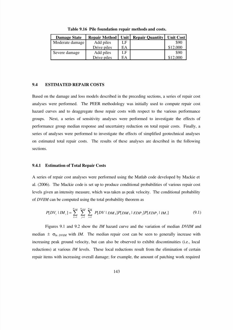
7/21/2019 PEER807 KRAMERArduino Shin
http://slidepdf.com/reader/full/peer807-kramerarduino-shin 155/198
143
Table 9.16 Pile foundation repair methods and costs.
Damage State Repair Method Unit Repair Quantity Unit Cost
Moderate damage Add pilesDrive piles
LFEA
$90$12,000
Severe damage Add pilesDrive piles
LFEA
$90$12,000
9.4 ESTIMATED REPAIR COSTS
Based on the damage and loss models described in the preceding sections, a series of repair cost
analyses were performed. The PEER methodology was initially used to compute repair cost
hazard curves and to deaggregate those repair costs with respect to the various performance
groups. Next, a series of sensitivity analyses were performed to investigate the effects of
performance group median response and uncertainty reduction on total repair costs. Finally, a
series of analyses were performed to investigate the effects of simplified geotechnical analyses
on estimated total repair costs. The results of these analyses are described in the following
sections.
9.4.1 Estimation of Total Repair Costs
A series of repair cost analyses were performed using the Matlab code developed by Mackie et
al. (2006). The Mackie code is set up to produce conditional probabilities of various repair cost
levels given an intensity measure, which was taken as peak velocity. The conditional probability
of DV | IM can be computed using the total probability theorem as
]|[]|[]|[]|[111
IM EDPP EDP DM P DM DV P IM DV P i j jk k
N
i
N
j
N
k
il
IM EDP DM
∑∑∑===
= (9.1)
Figures 9.1 and 9.2 show the IM hazard curve and the variation of median DV | IM and
median ± σln DV | IM with IM . The median repair cost can be seen to generally increase with
increasing peak ground velocity, but can also be observed to exhibit discontinuities (i.e., local
reductions) at various IM levels. These local reductions result from the elimination of certain
repair items with increasing overall damage; for example, the amount of patching work required
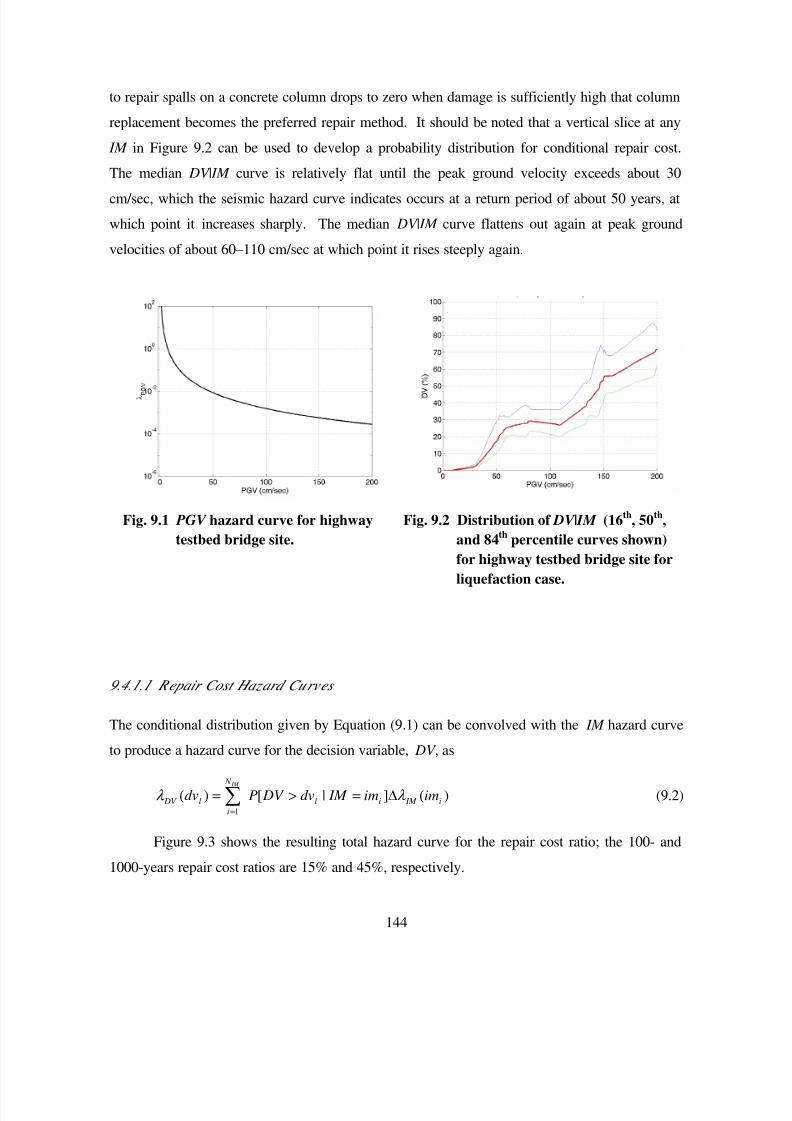
7/21/2019 PEER807 KRAMERArduino Shin
http://slidepdf.com/reader/full/peer807-kramerarduino-shin 156/198
144
to repair spalls on a concrete column drops to zero when damage is sufficiently high that column
replacement becomes the preferred repair method. It should be noted that a vertical slice at any
IM in Figure 9.2 can be used to develop a probability distribution for conditional repair cost.
The median DV | IM curve is relatively flat until the peak ground velocity exceeds about 30
cm/sec, which the seismic hazard curve indicates occurs at a return period of about 50 years, at
which point it increases sharply. The median DV | IM curve flattens out again at peak ground
velocities of about 60–110 cm/sec at which point it rises steeply again.
Fig. 9.1 PGV hazard curve for highway
testbed bridge site.
Fig. 9.2 Distribution of DV | IM (16th
, 50th
,
and 84th
percentile curves shown)
for highway testbed bridge site forliquefaction case.
9.4.1.1 Repair Cost Hazard Curves
The conditional distribution given by Equation (9.1) can be convolved with the IM hazard curve
to produce a hazard curve for the decision variable, DV , as
)(]|[)(1
i IM il
N
i
l DV imim IM dv DV Pdv IM
λ λ ∆=>=∑=
(9.2)
Figure 9.3 shows the resulting total hazard curve for the repair cost ratio; the 100- and
1000-years repair cost ratios are 15% and 45%, respectively.
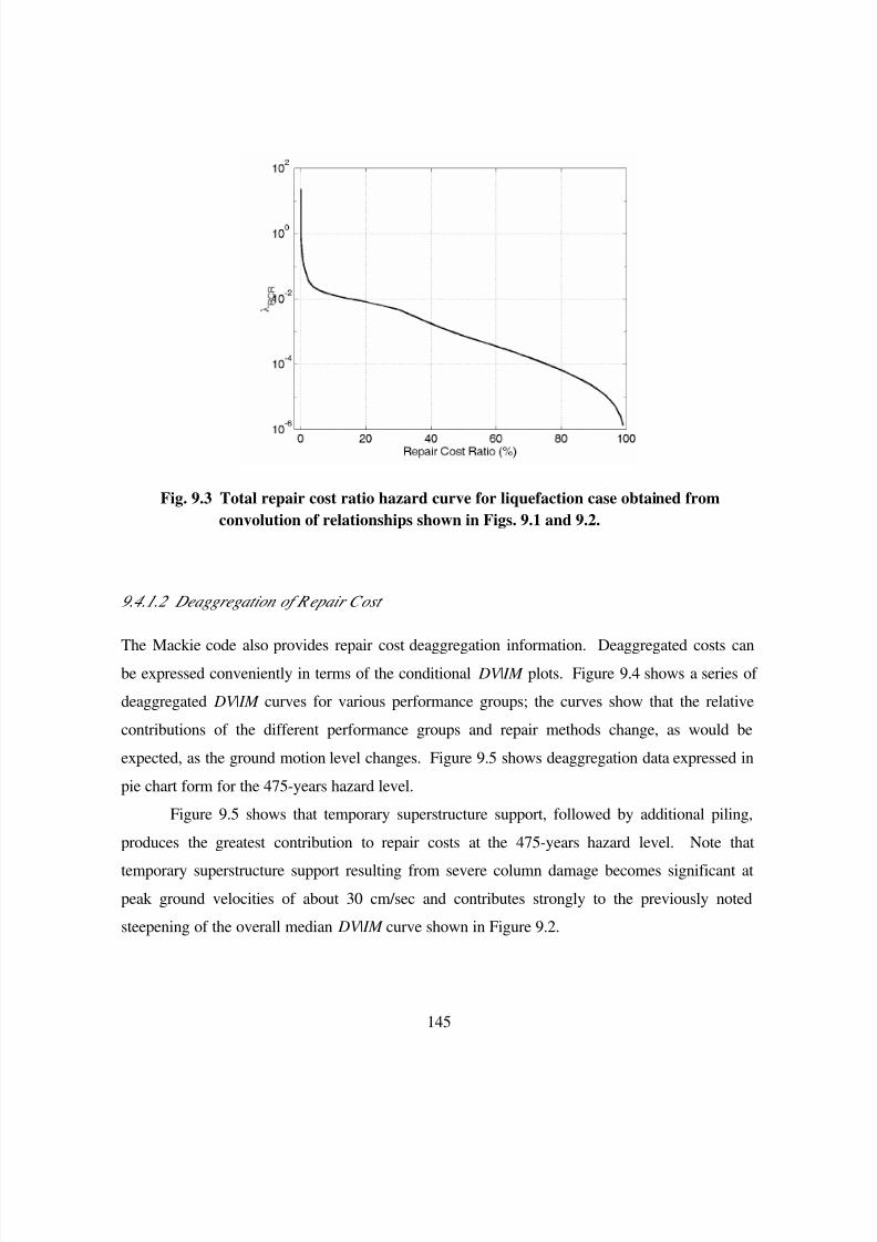
7/21/2019 PEER807 KRAMERArduino Shin
http://slidepdf.com/reader/full/peer807-kramerarduino-shin 157/198
145
Fig. 9.3 Total repair cost ratio hazard curve for liquefaction case obtained from
convolution of relationships shown in Figs. 9.1 and 9.2.
9.4.1.2
Deaggregation of R epair Cost
The Mackie code also provides repair cost deaggregation information. Deaggregated costs can
be expressed conveniently in terms of the conditional DV | IM plots. Figure 9.4 shows a series of
deaggregated DV | IM curves for various performance groups; the curves show that the relative
contributions of the different performance groups and repair methods change, as would be
expected, as the ground motion level changes. Figure 9.5 shows deaggregation data expressed in
pie chart form for the 475-years hazard level.
Figure 9.5 shows that temporary superstructure support, followed by additional piling,
produces the greatest contribution to repair costs at the 475-years hazard level. Note that
temporary superstructure support resulting from severe column damage becomes significant at
peak ground velocities of about 30 cm/sec and contributes strongly to the previously noted
steepening of the overall median DV | IM curve shown in Figure 9.2.
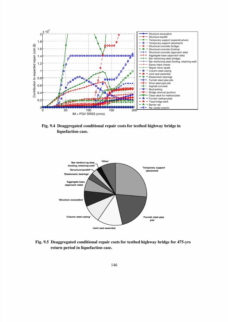
7/21/2019 PEER807 KRAMERArduino Shin
http://slidepdf.com/reader/full/peer807-kramerarduino-shin 158/198
146
0 50 100 150 2000
0.2
0.4
0.6
0.8
1
1.2
1.4
1.6
1.8
2x 10
5
IM = PGV SRSS (cm/s)
C o n t r i b u t i o n t o e x p e c t e d r e p a i r c
o s t ( $ )
Structure excavation
Structure backfill
Temporary support (superstructure)
Temporary support (abutment)
Structural concrete (bridge)
Structural concrete (footing)
Structural concrete (approach slab)
Aggregate base (approach slab)
Bar reinforcing steel (bridge)
Bar reinforcing steel (footing, retaining wall)
Epoxy inject cracks
Repair minor spalls
Column steel casing
Joint seal assembly
Elastomeric bearings
Furnish steel pipe pile
Drive steel pipe pile
Asphalt concrete
Mud jacking
Bridge removal (portion)
Clean deck for methacrylate
Furnish methacrylate
Treat bridge deck
Barrier rail
Re−center column
Fig. 9.4 Deaggregated conditional repair costs for testbed highway bridge in
liquefaction case.
'Temporary support
(abutment)'
'Furnish steel pipe
pile'
'Joint seal assembly'
'Column steel casing'
'Structure excavation'
'Aggregate base
(approach slab)'
'Elastomeric bearings'
'Structure backfill'
'Bar reinforcing steel
(footing, retaining wall)'
'Other'
Fig. 9.5 Deaggregated conditional repair costs for testbed highway bridge for 475-yrs
return period in liquefaction case.
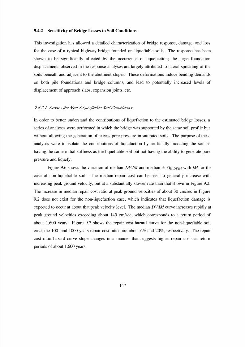
7/21/2019 PEER807 KRAMERArduino Shin
http://slidepdf.com/reader/full/peer807-kramerarduino-shin 159/198
147
9.4.2 Sensitivity of Bridge Losses to Soil Conditions
This investigation has allowed a detailed characterization of bridge response, damage, and loss
for the case of a typical highway bridge founded on liquefiable soils. The response has been
shown to be significantly affected by the occurrence of liquefaction; the large foundation
displacements observed in the response analyses are largely attributed to lateral spreading of the
soils beneath and adjacent to the abutment slopes. These deformations induce bending demands
on both pile foundations and bridge columns, and lead to potentially increased levels of
displacement of approach slabs, expansion joints, etc.
9.4.2.1
Losses for Non-L iquefiable Soil Conditions
In order to better understand the contributions of liquefaction to the estimated bridge losses, a
series of analyses were performed in which the bridge was supported by the same soil profile but
without allowing the generation of excess pore pressure in saturated soils. The purpose of these
analyses were to isolate the contributions of liquefaction by artificially modeling the soil as
having the same initial stiffness as the liquefiable soil but not having the ability to generate pore
pressure and liquefy.
Figure 9.6 shows the variation of median DV | IM and median ± σln DV | IM with IM for the
case of non-liquefiable soil. The median repair cost can be seen to generally increase with
increasing peak ground velocity, but at a substantially slower rate than that shown in Figure 9.2.
The increase in median repair cost ratio at peak ground velocities of about 30 cm/sec in Figure
9.2 does not exist for the non-liquefaction case, which indicates that liquefaction damage is
expected to occur at about that peak velocity level. The median DV | IM curve increases rapidly at
peak ground velocities exceeding about 140 cm/sec, which corresponds to a return period of
about 1,600 years. Figure 9.7 shows the repair cost hazard curve for the non-liquefiable soil
case; the 100- and 1000-years repair cost ratios are about 6% and 20%, respectively. The repaircost ratio hazard curve slope changes in a manner that suggests higher repair costs at return
periods of about 1,600 years.
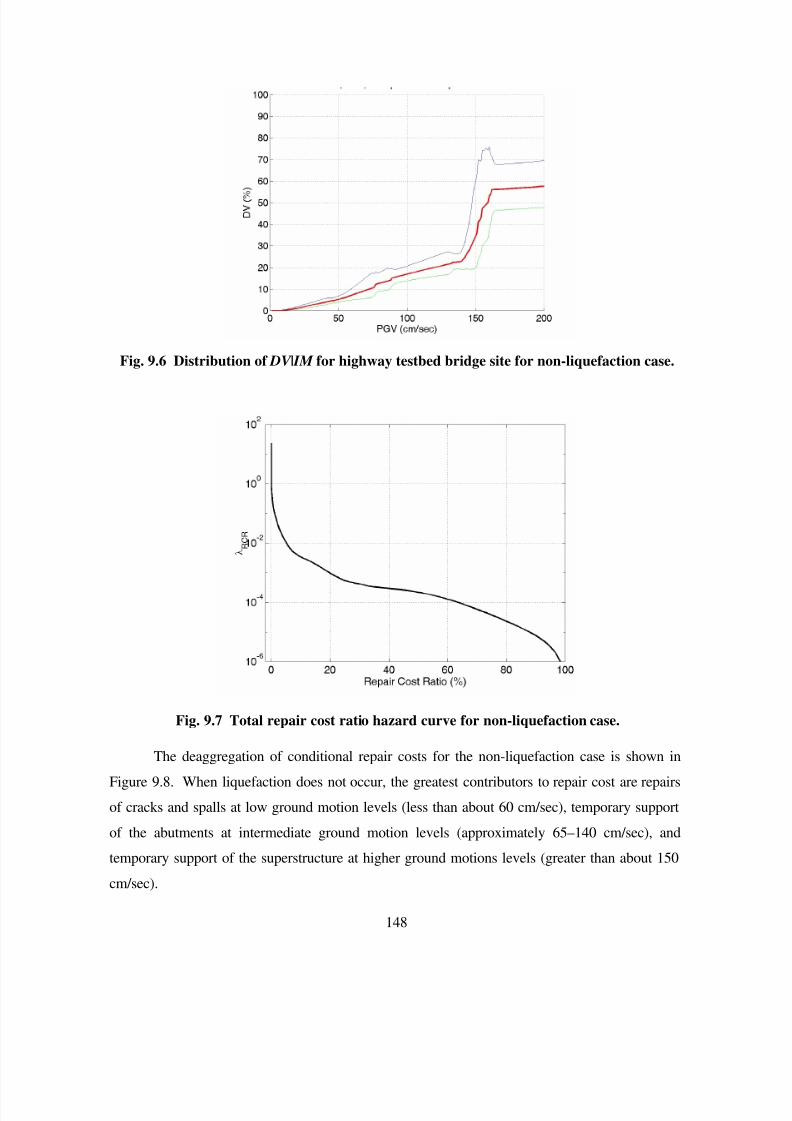
7/21/2019 PEER807 KRAMERArduino Shin
http://slidepdf.com/reader/full/peer807-kramerarduino-shin 160/198
148
Fig. 9.6 Distribution of DV | IM for highway testbed bridge site for non-liquefaction case.
Fig. 9.7 Total repair cost ratio hazard curve for non-liquefaction case.
The deaggregation of conditional repair costs for the non-liquefaction case is shown in
Figure 9.8. When liquefaction does not occur, the greatest contributors to repair cost are repairs
of cracks and spalls at low ground motion levels (less than about 60 cm/sec), temporary support
of the abutments at intermediate ground motion levels (approximately 65–140 cm/sec), and
temporary support of the superstructure at higher ground motions levels (greater than about 150
cm/sec).
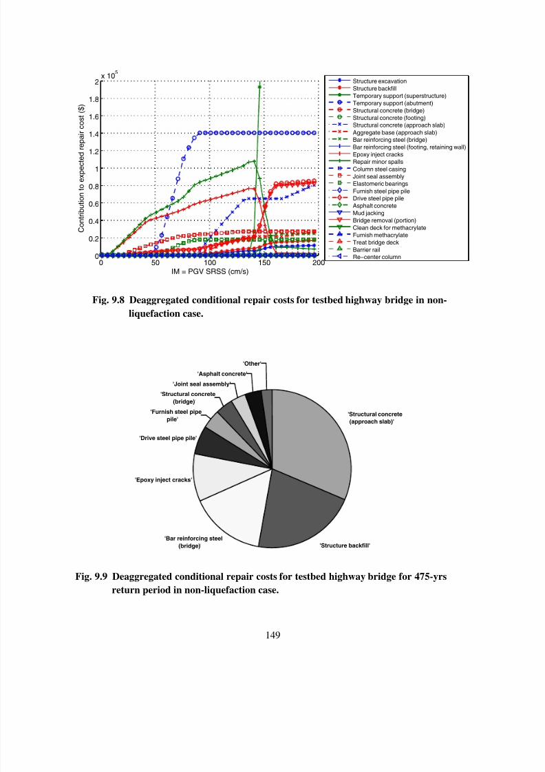
7/21/2019 PEER807 KRAMERArduino Shin
http://slidepdf.com/reader/full/peer807-kramerarduino-shin 161/198
149
0 50 100 150 2000
0.2
0.4
0.6
0.8
1
1.2
1.4
1.6
1.8
2x 10
5
IM = PGV SRSS (cm/s)
C o n t r i b u t i o n t o e x p e c t e d r e p a i r c o s t ( $ )
Structure excavation
Structure backfill
Temporary support (superstructure)
Temporary support (abutment)
Structural concrete (bridge)
Structural concrete (footing)
Structural concrete (approach slab)
Aggregate base (approach slab)
Bar reinforcing steel (bridge)
Bar reinforcing steel (footing, retaining wall)
Epoxy inject cracks
Repair minor spalls
Column steel casing
Joint seal assembly
Elastomeric bearings
Furnish steel pipe pile
Drive steel pipe pile
Asphalt concrete
Mud jacking
Bridge removal (portion)
Clean deck for methacrylate
Furnish methacrylate
Treat bridge deck
Barrier rail
Re−center column
Fig. 9.8 Deaggregated conditional repair costs for testbed highway bridge in non-
liquefaction case.
'Structural concrete
(approach slab)'
'Structure backfill'
'Bar reinforcing steel
(bridge)'
'Epoxy inject cracks'
'Drive steel pipe pile'
'Furnish steel pipe
pile'
'Structural concrete
(bridge)'
'Joint seal assembly'
'Asphalt concrete'
'Other'
Fig. 9.9 Deaggregated conditional repair costs for testbed highway bridge for 475-yrs
return period in non-liquefaction case.
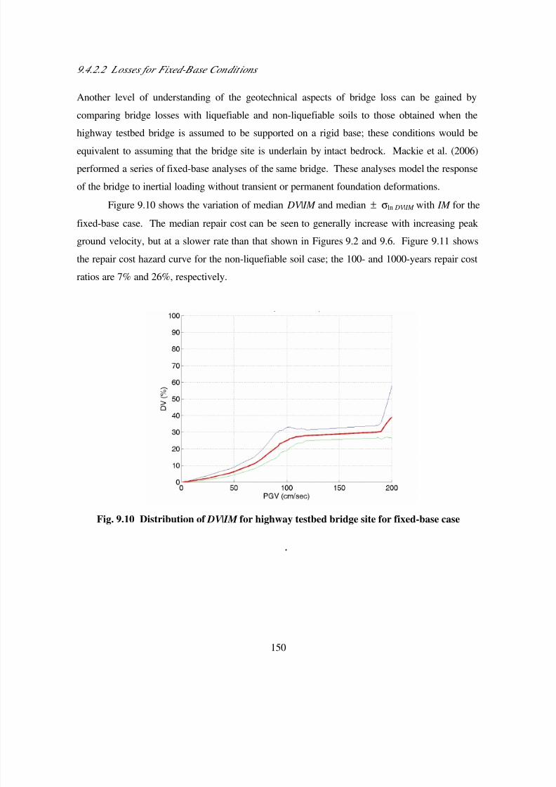
7/21/2019 PEER807 KRAMERArduino Shin
http://slidepdf.com/reader/full/peer807-kramerarduino-shin 162/198
150
9.4.2.2 Losses for Fixed-Base Conditions
Another level of understanding of the geotechnical aspects of bridge loss can be gained by
comparing bridge losses with liquefiable and non-liquefiable soils to those obtained when the
highway testbed bridge is assumed to be supported on a rigid base; these conditions would be
equivalent to assuming that the bridge site is underlain by intact bedrock. Mackie et al. (2006)
performed a series of fixed-base analyses of the same bridge. These analyses model the response
of the bridge to inertial loading without transient or permanent foundation deformations.
Figure 9.10 shows the variation of median DV | IM and median ± σln DV | IM with IM for the
fixed-base case. The median repair cost can be seen to generally increase with increasing peak
ground velocity, but at a slower rate than that shown in Figures 9.2 and 9.6. Figure 9.11 shows
the repair cost hazard curve for the non-liquefiable soil case; the 100- and 1000-years repair costratios are 7% and 26%, respectively.
Fig. 9.10 Distribution of DV | IM for highway testbed bridge site for fixed-base case
.
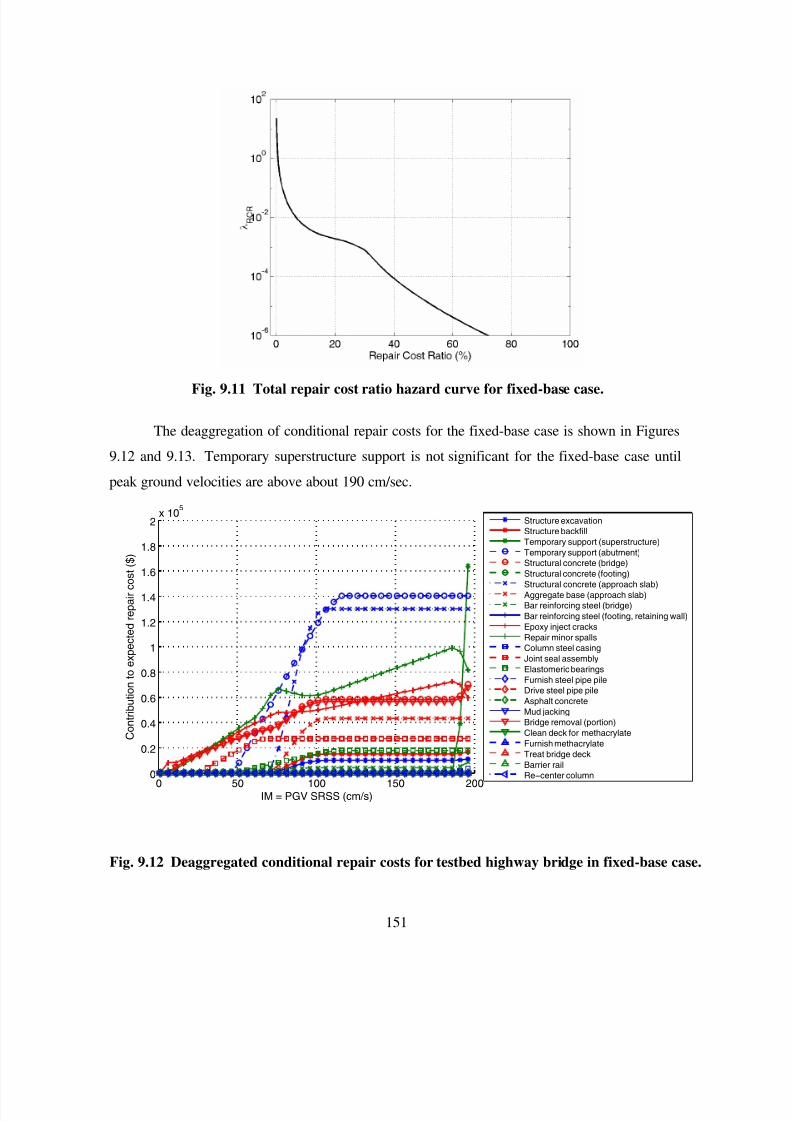
7/21/2019 PEER807 KRAMERArduino Shin
http://slidepdf.com/reader/full/peer807-kramerarduino-shin 163/198
151
Fig. 9.11 Total repair cost ratio hazard curve for fixed-base case.
The deaggregation of conditional repair costs for the fixed-base case is shown in Figures
9.12 and 9.13. Temporary superstructure support is not significant for the fixed-base case until
peak ground velocities are above about 190 cm/sec.
0 50 100 150 2000
0.2
0.4
0.6
0.8
1
1.2
1.4
1.6
1.8
2x 10
5
IM = PGV SRSS (cm/s)
C o n t r i b u t i o n t o e x p e c t e d r e p a i r c o s t ( $
)
Structure excavation
Structure backfill
Temporary support (superstructure)
Temporary support (abutment)
Structural concrete (bridge)Structural concrete (footing)
Structural concrete (approach slab)
Aggregate base (approach slab)
Bar reinforcing steel (bridge)
Bar reinforcing steel (footing, retaining wall)
Epoxy inject cracks
Repair minor spalls
Column steel casing
Joint seal assembly
Elastomeric bearings
Furnish steel pipe pile
Drive steel pipe pile
Asphalt concrete
Mud jacking
Bridge removal (portion)
Clean deck for methacrylate
Furnish methacrylate
Treat bridge deck
Barrier rail
Re−center column
Fig. 9.12 Deaggregated conditional repair costs for testbed highway bridge in fixed-base case.
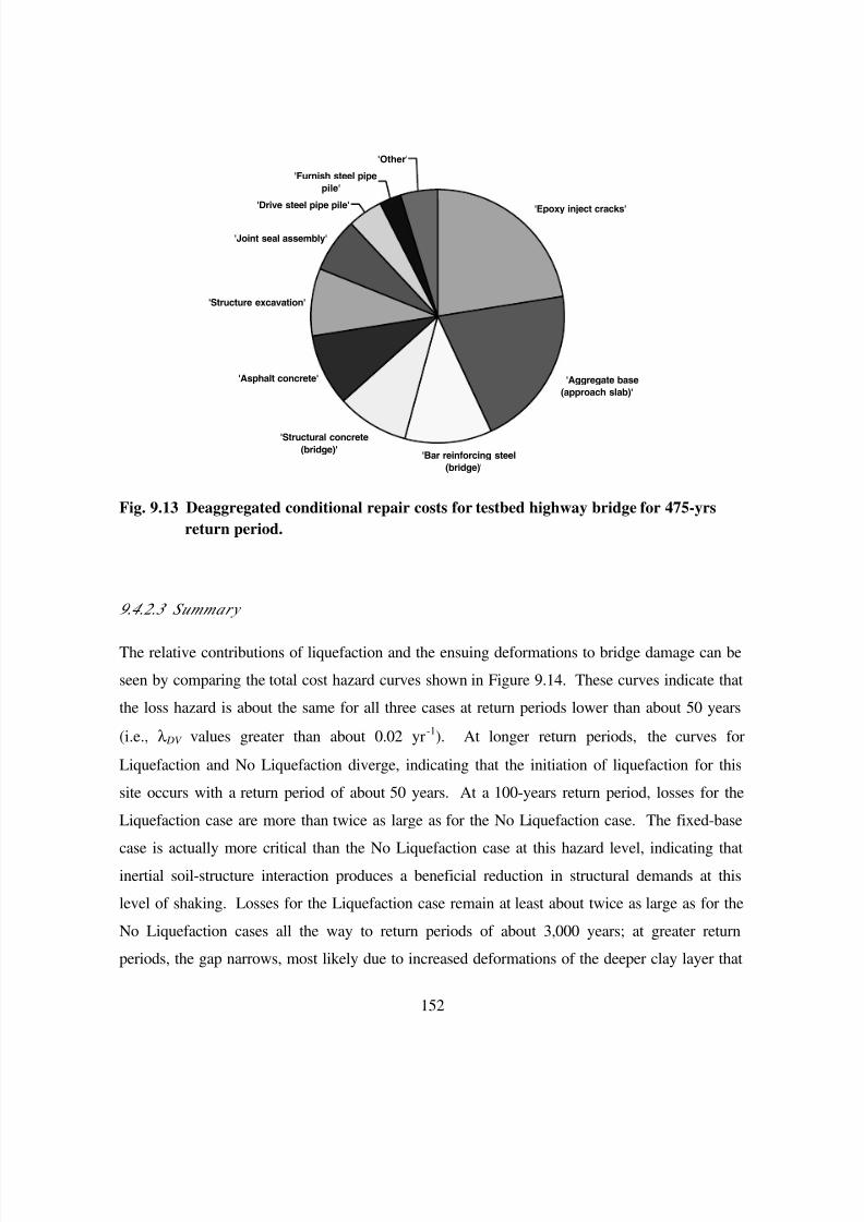
7/21/2019 PEER807 KRAMERArduino Shin
http://slidepdf.com/reader/full/peer807-kramerarduino-shin 164/198
152
'Epoxy inject cracks'
'Aggregate base
(approach slab)'
'Bar reinforcing steel
(bridge)'
'Structural concrete
(bridge)'
'Asphalt concrete'
'Structure excavation'
'Joint seal assembly'
'Drive steel pipe pile'
'Furnish steel pipe
pile'
'Other'
Fig. 9.13 Deaggregated conditional repair costs for testbed highway bridge for 475-yrs
return period.
9.4.2.3
Summary
The relative contributions of liquefaction and the ensuing deformations to bridge damage can be
seen by comparing the total cost hazard curves shown in Figure 9.14. These curves indicate that
the loss hazard is about the same for all three cases at return periods lower than about 50 years
(i.e., λ DV values greater than about 0.02 yr-1). At longer return periods, the curves for
Liquefaction and No Liquefaction diverge, indicating that the initiation of liquefaction for this
site occurs with a return period of about 50 years. At a 100-years return period, losses for the
Liquefaction case are more than twice as large as for the No Liquefaction case. The fixed-base
case is actually more critical than the No Liquefaction case at this hazard level, indicating that
inertial soil-structure interaction produces a beneficial reduction in structural demands at this
level of shaking. Losses for the Liquefaction case remain at least about twice as large as for the
No Liquefaction cases all the way to return periods of about 3,000 years; at greater return
periods, the gap narrows, most likely due to increased deformations of the deeper clay layer that
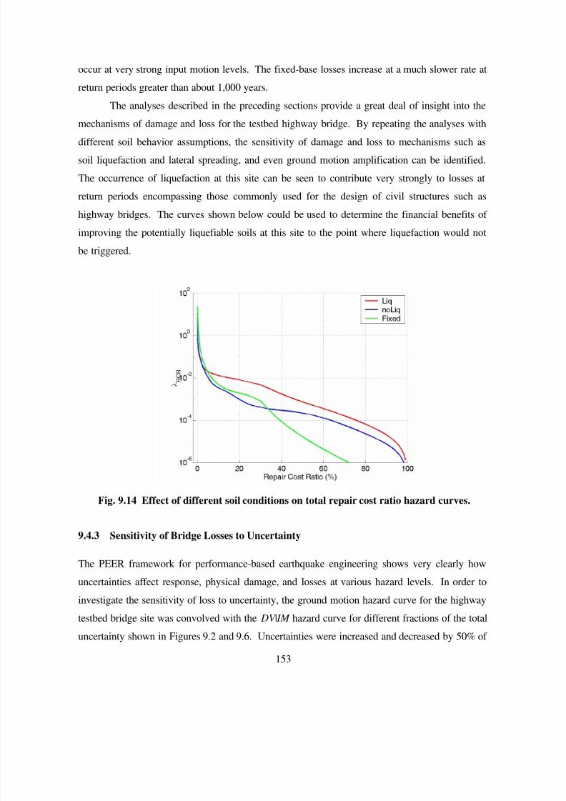
7/21/2019 PEER807 KRAMERArduino Shin
http://slidepdf.com/reader/full/peer807-kramerarduino-shin 165/198
153
occur at very strong input motion levels. The fixed-base losses increase at a much slower rate at
return periods greater than about 1,000 years.
The analyses described in the preceding sections provide a great deal of insight into the
mechanisms of damage and loss for the testbed highway bridge. By repeating the analyses with
different soil behavior assumptions, the sensitivity of damage and loss to mechanisms such as
soil liquefaction and lateral spreading, and even ground motion amplification can be identified.
The occurrence of liquefaction at this site can be seen to contribute very strongly to losses at
return periods encompassing those commonly used for the design of civil structures such as
highway bridges. The curves shown below could be used to determine the financial benefits of
improving the potentially liquefiable soils at this site to the point where liquefaction would not
be triggered.
Fig. 9.14 Effect of different soil conditions on total repair cost ratio hazard curves.
9.4.3 Sensitivity of Bridge Losses to Uncertainty
The PEER framework for performance-based earthquake engineering shows very clearly how
uncertainties affect response, physical damage, and losses at various hazard levels. In order to
investigate the sensitivity of loss to uncertainty, the ground motion hazard curve for the highway
testbed bridge site was convolved with the DV | IM hazard curve for different fractions of the total
uncertainty shown in Figures 9.2 and 9.6. Uncertainties were increased and decreased by 50% of
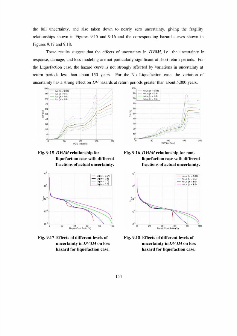
7/21/2019 PEER807 KRAMERArduino Shin
http://slidepdf.com/reader/full/peer807-kramerarduino-shin 166/198
154
the full uncertainty, and also taken down to nearly zero uncertainty, giving the fragility
relationships shown in Figures 9.15 and 9.16 and the corresponding hazard curves shown in
Figures 9.17 and 9.18.
These results suggest that the effects of uncertainty in DV | IM , i.e., the uncertainty in
response, damage, and loss modeling are not particularly significant at short return periods. For
the Liquefaction case, the hazard curve is not strongly affected by variations in uncertainty at
return periods less than about 150 years. For the No Liquefaction case, the variation of
uncertainty has a strong effect on DV hazards at return periods greater than about 5,000 years.
Fig. 9.15 DV | IM relationship for
liquefaction case with different
fractions of actual uncertainty.
Fig. 9.16 DV | IM relationship for non-
liquefaction case with different
fractions of actual uncertainty.
Fig. 9.17 Effects of different levels of
uncertainty in DV | IM on loss
hazard for liquefaction case.
Fig. 9.18 Effects of different levels of
uncertainty in DV | IM on loss
hazard for liquefaction case.
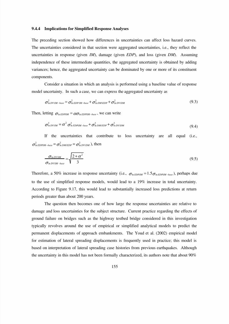
7/21/2019 PEER807 KRAMERArduino Shin
http://slidepdf.com/reader/full/peer807-kramerarduino-shin 167/198
155
9.4.4 Implications for Simplified Response Analyses
The preceding section showed how differences in uncertainties can affect loss hazard curves.
The uncertainties considered in that section were aggregated uncertainties, i.e., they reflect the
uncertainties in response (given IM ), damage (given EDP), and loss (given DM ). Assuming
independence of these intermediate quantities, the aggregated uncertainty is obtained by adding
variances; hence, the aggregated uncertainty can be dominated by one or more of its constituent
components.
Consider a situation in which an analysis is performed using a baseline value of response
model uncertainty. In such a case, we can express the aggregated uncertainty as
σ σ σ σ 2
|ln2
|ln2
|ln2
|ln DM DV EDP DM base IM EDPbase IM DV ++= −− (9.3)
Then, letting ασ σ base IM EDP IM EDP −= |ln|ln , we can write
σ σ σ α σ 2
|ln2
|ln2
|ln22
|ln DM DV EDP DM base IM EDP IM DV ++= − (9.4)
If the uncertainties that contribute to loss uncertainty are all equal (i.e.,
σ σ σ 2
|ln2
|ln2
|ln DM DV EDP DM base IM EDP ==− ), then
3
2 2
|ln
|ln α
σ
σ +=
−base IM DV
IM DV (9.5)
Therefore, a 50% increase in response uncertainty (i.e., σ σ base IM EDP IM EDP −= |ln|ln 5.1 ), perhaps due
to the use of simplified response models, would lead to a 19% increase in total uncertainty.
According to Figure 9.17, this would lead to substantially increased loss predictions at return
periods greater than about 200 years.
The question then becomes one of how large the response uncertainties are relative to
damage and loss uncertainties for the subject structure. Current practice regarding the effects of
ground failure on bridges such as the highway testbed bridge considered in this investigation
typically revolves around the use of empirical or simplified analytical models to predict the
permanent displacements of approach embankments. The Youd et al. (2002) empirical model
for estimation of lateral spreading displacements is frequently used in practice; this model is
based on interpretation of lateral spreading case histories from previous earthquakes. Although
the uncertainty in this model has not been formally characterized, its authors note that about 90%
7/21/2019 PEER807 KRAMERArduino Shin
http://slidepdf.com/reader/full/peer807-kramerarduino-shin 168/198
156
of its predicted displacement values fall within a factor of 2 of the observed values in the case
history database. Assuming that the values are lognormally distributed, this would correspond to
a dispersion of approximately σln EDP| IM = 0.6 in. the prediction of approach embankment
displacements. Newmark-type analyses are also used to estimate permanent slope
displacements, although their applicability to soils in which pore pressures are generated is not
straightforward. While no formal analyses of the uncertainty in such methods are available, the
simplifications involved in these methods, along with record-to-record variability and the manner
in which pore pressure generation is handled (or not handled) may well render their precision no
better than the empirical methods.
The biggest difference between such simplified analyses and the detailed analyses
conducted as part of this investigation, however, lies in the amount of information available to
predict physical damage. In the detailed investigation, some 27 EDPs were explicitly calculated
by OpenSees analysis and used to predict the required DM s. In simplified analyses, only two
EDPs (the approach embankment displacements) are available for prediction of damage; some of
the important damage mechanisms, however, are not related particularly closely to approach
embankment displacements.
In order to obtain a sense of how much the additional information provided by a detailed
analysis might improve loss estimates compared to a simplified analysis, a simple parametric
analysis was performed. In this analysis, the uncertainties in response (i.e., σln EDP| IM ) used in thepreviously described detailed analyses (Section 9.2) were adjusted to reflect the additional
uncertainty that could exist in DV | IM if the EDPs were limited to approach embankment
permanent displacements. The results of these analyses showed that the uncertainty in computed
response was dominated by the uncertainties in damage (given response) and loss (given
damage). In the end, with loss as the final metric of performance, the reduced uncertainty due to
more accurate response modeling (given the assumption of equal median predictions) had a
negligible effect on predicted losses. The analyses clearly showed, however, that errors in
median response, as might be expected from simple analyses, would have a significant effect on
computed losses; errors in median response, however, could not be predicted for the hypothetical
testbed structure.
7/21/2019 PEER807 KRAMERArduino Shin
http://slidepdf.com/reader/full/peer807-kramerarduino-shin 169/198
157
9.5 SUMMARY
This chapter illustrated the process by which earthquake-related losses could be estimated for the
testbed bridge structure using the PEER PBEE methodology. The methodology was found to be
effective in allowing estimation of loss hazard curves with consideration of uncertainties in
ground motions, response, damage, and loss. The losses associated with liquefaction-induced
deformations were included by explicitly modeling the liquefaction process, and the interaction
of the structure with liquefied soils, using the OpenSees computer model.
By condensing the results of the response, damage, and loss model analyses, fragility
curves for loss given ground motion intensity, i.e., DV | IM , could be computed. These fragility
curves could then be combined with the seismic hazard curve to produce loss curves. The
fragility curves showed a relatively irregular increase in loss with increasing intensity measure,thereby reflecting the onset and effects of physical phenomena such as liquefaction and shear
failure. Response analyses were computed for cases in which liquefaction was modeled, and for
which it was suppressed, and for a fixed-base support condition. Loss curves were computed for
each of these cases.
Loss curves for each of the three cases reflect the physical mechanisms that lead to
damage and loss under the various assumptions, and provide insight into the overall behavior of
the soil-foundation-structure system. The loss curves exhibit irregular changes in slope, and
consequently in shape, due to the irregularities in the DV | IM fragility curves. The loss curve for
the case in which liquefaction occurred, for example, becomes flatter at a return period of about
50 years due to the occurrence of liquefaction-related damage when ground motions reach
sufficiently strong levels. In the case in which liquefaction was suppressed, the loss curve
becomes flatter at a return period of about 1,600 years, which is when highly nonlinear response
of the clay layer beneath the left side of the bridge begins to develop.
Earthquake-related losses are shown to be influenced by uncertainties in the prediction of
ground motions, system response, physical damage, and economic loss. Uncertainties in ground
motions are accounted for by a probabilistic seismic hazard analysis, which forms the input to a
performance-based earthquake engineering evaluation. Uncertainties in response are related to
uncertainties in the parameters required for response predictions and in the predictive models
themselves. Different levels of response analysis require different input parameters and have
different levels of model uncertainty; however, the model uncertainty inherent in either

7/21/2019 PEER807 KRAMERArduino Shin
http://slidepdf.com/reader/full/peer807-kramerarduino-shin 170/198
158
simplified or detailed analyses has not been formally established. Nevertheless, it seems logical
that detailed analyses will produce response estimates to which damage is more closely related
than simplified analyses. When uncertainties in damage and loss estimation are large, however,
the effects of different levels of uncertainty in response analyses may not have a significant
effect on loss curves. This appears to be the case for the conditions studied in the analysis of the
subject testbed bridge structure.
7/21/2019 PEER807 KRAMERArduino Shin
http://slidepdf.com/reader/full/peer807-kramerarduino-shin 171/198
159
10 Summary and Conclusions
Performance-based earthquake engineering provides for the prediction of seismic performance of
structures and facilities in terms that are useful to various stakeholders. The performance-based
framework developed by PEER allows description of performance in terms that are useful to
earth scientists, engineers, loss analysts, and facility owners/operators. It accounts for ground
motions, system response, physical damage, and related losses in a systematic fashion that
accounts for uncertainties in all of these factors. The primary goal of the research described in
this report was to illustrate the manner in which the PEER framework could be used to evaluate
the performance of a bridge underlain by liquefiable soils.
A detailed performance evaluation was undertaken for a hypothetical, but realistic,
highway bridge founded on liquefaction-susceptible soils. Such conditions are relatively
common for bridges in seismically active areas, but response has historically been difficult to
evaluate using available computational tools. As a result, response evaluations have typically
been performed using empirical or simplified computational models. The output of such models
is limited, so their use in the direct estimation of physical damage is fraught with uncertainty. As
a result, estimates of loss based on such estimates of physical damage are also affected by these
high levels of uncertainty.
The detailed performance evaluation was based on response computations using the
OpenSees computational platform; OpenSees allows high-level modeling of both the structural
and geotechnical components of a bridge and its foundations, which then allows direct estimation
of response variables to which physical damage is related. As a result, subsequent loss estimates
can be based upon more accurate measures of physical damage.
7/21/2019 PEER807 KRAMERArduino Shin
http://slidepdf.com/reader/full/peer807-kramerarduino-shin 172/198
160
10.1 SUMMARY
Following reviews of the basic concepts of performance-based earthquake engineering and soil-
pile-structure interaction, a hypothetical highway testbed bridge and soil profile was defined.
The bridge superstructure was taken to be identical to that analyzed under fixed-based conditions
by Mackie and Stojadinović (2006). The soil profile was developed in coordination with Prof.
Jonathan Bray and Dr. Christian Ledezma of UC Berkeley who were carrying out a parallel
project based on the use of empirical and simplified analyses on the same bridge-soil system.
The soil profile beneath the hypothetical testbed bridge included a shallow layer of liquefaction-
susceptible soil of variable thickness. The liquefiable layer was thicker beneath the right
abutment than the left abutment, but lateral spreading hazards were anticipated beneath bothabutments and bridge approaches. The pile foundations required to support the bridge on the
selected soil profile were designed by Dr. Ledezma.
The response of the bridge to earthquake loading was analyzed using a detailed OpenSees
finite element model. The model captured details of the structural response, such as bearing
response, abutment wall break-off, girder-abutment impact, etc., which are often not explicitly
modeled in analyses that include soil response. The model also captured details of the
geotechnical response, such as phase transformation behavior in liquefiable soils, nonlinear,
inelastic pile-soil interaction, permanent soil deformations, etc., which are often not explicitly
modeled in analyses that include structural response. While the OpenSees modeling effort went
considerably beyond that normally used in contemporary practice, it provides a view of the types
of analyses that are likely to become practical in the relatively near future.
The computed response was used to estimate various forms of physical damage, which
were each divided into different damage states. The cost of repair for each damage state was
then estimated. Convolving the response, damage, and loss models with a ground motion hazard
curve allowed estimation of repair cost hazard curves. Cost hazard curves were also developed
for cases in which pore pressure generation in potentially liquefiable soils was restricted; the
difference between the cost curves with and without pore pressure generation provides insight
into the effects of liquefaction on estimated repair costs. Repair cost curves were also generated
for the fixed base model to allow the estimation of repair costs based solely on shaking-induced
structural damage.
7/21/2019 PEER807 KRAMERArduino Shin
http://slidepdf.com/reader/full/peer807-kramerarduino-shin 173/198
161
The research described in this report provides useful insights into the conceptual and
practical factors that influence performance-based earthquake engineering evaluations, and
demonstrates the benefits of performing such evaluations. By performing detailed response
analyses, the EDPs that relate most closely to physical damage, and hence to repair costs, could
be explicitly computed. The primary conclusions that could be drawn from this investigation
include:
1. The occurrence of liquefaction can cause sharply increased losses for a bridge subject to
lateral spreading hazards. The analyses performed in this research investigation showed
that losses associated with liquefaction-induced permanent soil deformations were
substantial. At even moderate return periods, losses were essentially doubled by the
occurrence of liquefaction.
2. Detailed modeling of soil-foundation-structure systems can provide more extensive and
more accurate estimates of system response, which lead to improved damage and loss
estimates. The additional uncertainty in response that comes with the use of simplified
response models leads to higher damage and loss estimates for a given hazard level. The
extent to which eventual loss estimates are influenced by the accuracy of response
estimates depends on the sensitivity of damage to response and of loss to damage, which
vary from site-to-site and structure-to-structure.
3. Selection of optimal IMs can lead to significant reductions in EDP uncertainty,
particularly for aspects of response related to soil liquefaction. The basic concept that
response hazards are sensitive to the uncertainty in response predictions is well
established. The resulting goal of working with IM s that are better predictors of response
than other IM s follows naturally from that concept. The analyses performed in this
investigation showed substantial differences in liquefaction-related EDP hazards when
predicted by different IM s.
4. Liquefaction-related hazards are better predicted by velocity-related IMs than
acceleration-related IMs. Response analyses performed for some 40 input motions
representing four different IM hazard levels showed that velocity-related IM s such as
peak ground velocity, Arias intensity, and CAV5 were significantly more efficient
predictors of response than peak ground acceleration. This observation is consistent with
the known facts that pore pressure generation in liquefiable soils is more closely related
7/21/2019 PEER807 KRAMERArduino Shin
http://slidepdf.com/reader/full/peer807-kramerarduino-shin 174/198
162
to shear strain than shear stress, and that shear strain amplitudes are proportional to
particle velocity in basic (linear) wave propagation.
5. The use of detailed soil-foundation-structure interaction analyses can lead to useful
insights into system behavior . The response of a soil-foundation-structure system such as
the highway testbed bridge studied in this investigation is complex and multi-faceted.
Certain aspects of the response to certain input motions were strongly affected by
interaction of all of the bridge/soil components. For example, the leftward lateral
translation of the bridge deck observed in response to some input motions caused column
drift ratios on the left side of the bridge to be greater than those on the right side even
though the lateral spreading displacements on the right side of the bridge were greater
than those on the left.
6. Power law relationships can provide a good approximation to IM-EDP relationships
even for complex soil-foundation-structure systems. Relatively simple power law
relationships were found to provide good median fits to EDP- IM data generated from
extensive series of OpenSees analyses.
7. Residuals from power law fits to response data were approximately lognormally
distributed. The residuals of EDP| IM from extensive series of OpenSees analyses were
observed to be approximately lognormally distributed. This observation, along with that
described in Item 4 above, allows the development of useful closed-form solutions for the
EDP hazard.
8. Record-to-record variability dominates the computation of response hazards.
Investigation of the effects of parametric uncertainty and spatial variability of soil
properties showed that their contribution to response hazards was much lower than that of
record-to-record variability. This emphasizes the importance of using efficient and
sufficient IM s for response estimation, and of paying close attention to the selection and
scaling of input motions for response analyses.
7/21/2019 PEER807 KRAMERArduino Shin
http://slidepdf.com/reader/full/peer807-kramerarduino-shin 175/198
163
REFERENCES
Abdoun T., Dobry R., O'Rourke T.O., and Goh S.H. (2003). Pile response to lateral spreads:
Centrifuge modeling. Journal of Geotechnical and Geoenvironmental Engineering, ASCE ,Vol. 129(No. 10):869–878.
API (1993). Recommended practice for planning, designing and constructing offshore platforms.
API Recommended Practice 2A (RP 2A), 20th Edition, Washington, D.C.
Arulanandan R., Boulanger R.W., Kutter B.L., and Sluis W.K. (2000). New tool for shear wave
velocity measurements in model tests. Geotechnical testing journal, Vol. 23(No. 4):444–453.
Baecher G.B. and Christian J.T. (2003). Reliability and Statistics in Geotechnical Engineering.
Prentice-Hall.
Barton Y.O. and Finn W.D.L. (1983). Lateral pile response and p-y curves from centrifuge tests.
Proceedings of the 15th Annual Offshore Technology Conference, Houston, Texas, (Paper
4502):503–508.
Berber T.M. and Rollins K.M. (2005). Lateral subgrade moduli for liquefied sand under cyclic
loading. Seismic Performance and Simulation of Pile Foundations in Liquefied and Laterally
Spreading Ground, Geotechnical Special Publication, (No. 145):149–160.
Berry M.P. and Eberhard M.O. (2003). Performance models for flexural damage in reinforced
concrete columns. PEER Report No. 2003/18. Pacific Earthquake Engineering Research
Center, University of California, Berkeley.
Boulanger R.W., Chang D., Gulerce U., Brandenberg S.J., and Kutter B.L. (2005). Evaluation
pile pinning effects on abutments over liquefied ground. Seismic Performance and
Simulation of Pile Foundations in Liquefied and Laterally Spreading Ground, Geotechnical
Special Publication, (No. 145):306–318.
Boulanger R.W., Curras C.J., Kutter B.L., D.W. Wilson, and A. Abghari (1999). Seismic soil-
pile-structure interaction experiments and analysis. Journal of Geotechnical and
Geoenvironmental Engineering, ASCE , Vol. 125(No. 9):750–759.
Boulanger R.W., Wilson D.W., Kutter B.L., Brandenberg S.J., and Chang D. (2004). Nonlinear
FE analysis of soil-pile-interaction liquefying sand. Proceedings, Geotechnical Engineering
for Transportation Projects, Geotechnical Special Publication, (No. 126): 470–478.

7/21/2019 PEER807 KRAMERArduino Shin
http://slidepdf.com/reader/full/peer807-kramerarduino-shin 176/198
164
Brandenberg S.J., Boulanger R.W., Kutter B.L., and Chang D. (2005). Behavior of pile
foundations in laterally spreading ground during centrifuge tests. Journal of Geotechnical
and Geoenvironmental Engineering, ASCE , Vol. 131(No. 11):1378–1391.
Brandenberg S.J. (2005). Behavior of Pile Foundations in Liquefied and Laterally Spreading
Ground . Ph.D. thesis, University of California, Davis.
Briaud J.-L. and Smith T.D. (1983). Using the pressuremeter curve to design laterally loaded
piles. Proceedings of the 15th Annual Offshore Technology Conference, Houston, Texas,
(Paper 4502):495–502.
Broms B.B. (1964). Lateral resistance of piles in cohesionless soils. Journal of Soil Mechanics
and Foundations Division, Vol. 90(SM3):123–156.
Broms B.B. (1964). Lateral resistance of piles in cohesive soils. Journal of Soil Mechanics and
Foundations Division, Vol. 90(SM2):27–63.
Brown D.A., Morrison C., and Reese L.C (1988). Lateral load behavior of pile group in sand.
Journal of Geotechnical and Geoenvironmental Engineering, ASCE , Vol. 114(No. 11):1261–
1276.
Caltrans (2004). Caltrans seismic design criteria.
Caltrans, (2004). Construction Statistics Based on Bid Openings, 2004. California
Department of Transportation, Division of Engineering Services.
http://www.dot.ca.gov/hq/esc/estimates/Construction_Stats_2004.xls
Caltrans, (2005). Comparative Bridge Costs, January 2005. California Department of
Transportation, Division of Structure Earthquake Engineering & Design Support
Castello R.R. (1980). Bearing Capacity of Driven Piles in Sand . PhD thesis, Texas AM
University, College Station, Texas.
Chai Y.H. (2002). Flexural strength and ductility of extended pile-shafts. i: Analytical model.
Journal of Structural Engineering, Vol. 128(No. 5):586–594.
Chai Y.H. and Hutchinson T.C. (2002). Flexural strength and ductility of extended pile-shafts. ii:
Experimental study. Journal of Structural Engineering, Vol. 128(No. 5):595–602.
Cordova P. (2000). Development of a two-parameter seismic intensity measure and probabilistic
seismic assessment procedure. PEER Report No.2000/10, 195–214. Pacific Earthquake
Engineering Research Center, University of California, Berkeley.
7/21/2019 PEER807 KRAMERArduino Shin
http://slidepdf.com/reader/full/peer807-kramerarduino-shin 177/198
165
Cornell C. A. and Krawinkler H. (2000). Progress and challenges in seismic performance
assessment. PEER News, April, pages 1–3.
Coyle H. and Castello R. (1981). New design correlations for piles in sand. Journal of
Geotechnical Engineering Division, ASCE , Vol. 107(No. GT7).
Coyle H.M and Sulaiman I.H. (1967). Skin friction for steel piles in sand. Journal of the Soil
Mechanics and Foundation Division, ASCE , Vol. 93(No. Sm-6).
Curras C.J., Boulanger R.W., Kutter B.L., and Wilson D.W. (2001). Dynamic experiences and
analysis of a pile-group-supported structure. Journal of Geotechnical and Geoenvironmental
Engineering, ASCE , Vol. 127(No. 7):585–596.
Deierlein G.G., Krawinkler H., and Cornell C.A. (2003). A framework for performance-based
earthquake engineering. Proceedings, 2003 Pacific Conference on Earthquake Engineering.
Dobry R., Taboada V., and Liu L. (1995). Centrifuge modeling of liquefaction effects during
earthquakes. Proc. 1st Intl. Conf. on Earthquake Geotechnical Engineering, K. Ishihara, ed.,
Tokyo, Japan, Vol. 3:1291–1324.
Duncan J.M. (2000). Factors of safety and reliability in geotechnical engineering. Journal of
Geotechnical and Geoenvironmental Engineering, ASCE , Vol. 126(No. 4):307–316.
Fleming W.G.K., Weltman A.J., and Randolph M.F. (1992). Piling engineering. Surrey
University Press, London.
Gazetas G. and Mylonakis G. (1998). Seismic soil-structure interaction: New evidence and
emerging issues. Geotechnical Earthquake Engineering and Soil Dynamics III, Geotechnical
Special Publication, Vol. 2(No. 75): 1119–1174.
Gerolymos N. and Gazetas G. (2005). Phenomenological model applied to inelastic response of
soil-pile interaction systems. Soil and Foundations, Vol. 45(No. 4): 119–132.
Hamada M. (1992). Large ground deformations and their effects on lifelines: 1964 Nigata
earthquake. Case Studies of Liquefaction and Lifeline Performance During Past
Earthquakes, Japanese Case Studies. Technical Report NCEER-92-0001, NCEER, Buffalo,
NY, USA., Vol. (1), 3.1–3.123.
Harr M.E. (1987). Reliability-Based Design in Civil Engineering. McGraw-Hill.
He L., Elgamal A., Abdoun T., Dobry R., Meneses J., Sato M., and Tokimatsu K. (2006). Lateral
load on piles due to liquefaction-induced lateral spreading during one-g shake table
experiments. Proceedings of 8th National Conference on Earthquake Engineering, San
Francisco, August 2006 .
7/21/2019 PEER807 KRAMERArduino Shin
http://slidepdf.com/reader/full/peer807-kramerarduino-shin 178/198
166
Hose Y., Silva P., and Seible F. (2000). Development of a performance evaluation database for
concrete bridge components and systems under simulated seismic loads. Earthquake Spectra,
Vol. 16(No. 2):413–442.
Ilankatharan M., Kutter B., Shin H., Arduino P., and Kramer S.L. ( 2007). A demonstration of
NEES system for studying soil-foundation-structure interaction: Centrifuge data report for
test series mil02. and Environmental Engineering, University of California, Davis,
California.
Ilankatharan M., Kutter B., Shin H., Arduino P., and Kramer S.L. ( 2007). A demonstration of
NEES system for studying soil-foundation-structure interaction: Centrifuge data report for
test series mil03. and Environmental Engineering, University of California, Davis,
California.
Ilankatharan M., Kutter B.L., Shin H., Arduino P., Kramer S.L., Johnson N., and Sasaki T.
(2006). Comparison of centrifuge and 1 g shake table models of a pile supported bridge
structure. Proceedings of the International Conference on Physical Modeling in Geotechnics,
August .
Ilankatharan M., Sasaki T., Shin H., Kutter B., Arduino P., and Kramer S.L. (2005). A
demonstration of NEES system for studying soil-foundation-structure interaction: Centrifuge
data report for test series mil01. Rep. No. UCD/CGMDR-05/05, Ctr. for Geotech. Modeling,
Dept. of civil and Environmental Engineering, University of California, Davis, California.
Jalayer F. (2003). Direct probabilistic Seismic Analysis: Implementating non-linear dynamic
assessments. PhD thesis, Stanford University, Stanford, California.
Johnson N., Saiidi M., and Sanders D. (2006). Large-scale experimental and analytical seismic
studies of a two-span reinforced concrete bridge system. Technical Report CCEER-06-02,
University of Nevada, Reno.
Jones A.L., Kramer S.L., and Arduino P. (2002). Estimation of uncertainty in geotechnical
properties for performance-base earthquake engineering. PEER Report No.2002/16, Pacific
Earthquake Engineering Research Center, University of California, Berkeley.
JRA (2002). Specifications for highway bridges. Japan Road Association, Preliminary English
Version, prepared by Public Works Research Institute (PWRI) and Civil Engineering
Research Laboratory (CRL), Japan, November.
7/21/2019 PEER807 KRAMERArduino Shin
http://slidepdf.com/reader/full/peer807-kramerarduino-shin 179/198
167
Juirnarongrit T. and Ashford S.A. (2004). Analyses of pile responses based on results from full-
scale lateral spreading test: Tokachi blast experiment. Proceedings of 13th World Conference
on Earthquake Engineering, Vancouver, Canada, August 1–6 .
Kawamata Y., Ashford S.A., and Juirnarongrit T. (2006). Numerical simulation of deep
foundations subjected to lateral spreading for Tokachi blast test. Proceedings of 8th National
Conference on Earthquake Engineering, San Francisco, August 2006 .
Kerisel J. (1964). Deep foundations, basic experimental facts. Proceedings, Conference on Deep
Foundations, Mexican Society of Soil Mechanics, Mexico City, Mexico, Vol.1, p.5.
Ketchum M., Chang V., and Shantz T. (2004). Influence of design ground motion level on
highway bridge cost. PEER Lifelines Project Number 6D01 Report, Pacific Earthquake
Engineering Research Center, University of California, Berkeley.
Kramer S.L. (1996). Geotechnical Earthquake Engineering. Prentice-Hall.
Kramer S.L. (2006). Personal communications.
Kramer S.L. and Mitchell R.A. (2006). Ground motion intensity measures for liquefaction
hazard evaluation. Earthquake Spectra, Vol. 22(No. 2).
Krawinkler H. (2002). A general approach to seismic performance assessment. Proceedings,
International Conference on Advances and New Challenges in Earthquake Engineering
Research (ICANCEER), Hong Kong.
Krawinkler H. and Miranda E. (2004). Performance-based earthquake engineering. In Bozorgnia
Y. and Bertero V., editors, Earthquake Engineering from Engineering Seismology to
Performance-Based Earthquake Engineering. CRC Press.
Kulhawy F.H. (1992). On the evaluation of static soil properties. ASCE Geotechnical Special
Publication, (No. 31):95–115.
Lacasse S. and Nadim F. (1996). Uncertainties in characterizing soil properties (plenary),
uncertainty in the geologic environment, from theory to practice. Proceeding of Uncertainty
’96, Geotechnical Special Publication No.58 .
Ledezma C.A. and Bray J.D. (2006). Peer bridge design of piles under the abutment.
Ledezma C.A. and Bray J.D. (2006). Peer bridge pile design report.
Ledezma, C.A. and Bray, J.D. (2007). “Performance-Based Earthquake Engineering Design
Evaluation Procedure for Bridge Foundations Undergoing Liquefaction-Induced Lateral
Spreading” PEER Report 2007/xx, Pacific Earthquake Engineering Research Center,
Berkeley, California, 150 pp.
7/21/2019 PEER807 KRAMERArduino Shin
http://slidepdf.com/reader/full/peer807-kramerarduino-shin 180/198
168
Luco N. and Cornell C.A. (2001). Structure-specific scalar intensity measures for near-source
and ordinary earthquake ground motions. Earthquake Spectra. Submitted for publication.
Mackie K and Stojadinović B. (2003). Seismic demands for performance-based design of
bridges. PEER Report No. 2003/16. Pacific Earthquake Engineering Research Center,
University of California, Berkeley.
Mackie K and Stojadinović B. (2005). Simplified application of the PEER methodology.
http://dodo.ce.berkeley.edu/mackie/Yr8/.
Mackie K., Wong J-M., and Stojadinović B. (2004). Method for post-earthquake highway
bridge repair cost estimation. Proceedings of 5th National Seismic Conference on Bridges
and Highways, San Mateo, CA.
Mackie K.R. and Stojadinović B. (2005). Comparison of incremental dynamic, cloud, and stripe
methods for computing probabilistic seismic demand models. In Proceedings of the 2005
ASCE Structures Congress, April 20–24, New York, NY .
Mackie, K., Wong, J-M., and Stojadinović, B. (2006). " Method for post-earthquake highway
bridge repair cost estimation." In Proceedings of the 5th National Seismic Conference on
Bridges and Highways, September 18–20. San Francisco, CA.
Mackie, K., and Stojadinović B, (2007). “Performance of Benchmark Bridge Structures,” ASCE
Structures Congress, Long Beach, CA. May 16–19 2007.
Mackie, K.R., Wong, J.-M., Stojadinović, B. (2007). “Integrated Probabilistic Performance-
Based Evaluation of Benchmark Reinforced Concrete Bridges,” PEER Report 2007/xx,
Pacific Earthquake Engineering Research Center, Berkeley, California, 202 pp
Makido A. (2007). Behavior of Spirally Reinforced Concrete Columns under Load Reversals.
PhD thesis, Purdue University.
Maroney B.H. (1995). Large scale bridge abutment tests to determine stiffness and ultimate
strength under seismic loading. Ph.D. thesis, University of California, Davis, CA.
Matlock H. (1970). Correlations for design of laterally loaded piles in soft clay. Proceedings of
the II Annual Offshore Technology Conference, Houston, Texas, (OTC 1204):577–594.
Mokwa R.L. (1999). Investigation of the Resistance of Pile Caps to Lateral Loading. Ph.D.
thesis, Virginia Polytechnic Institute.
Mosher R.L (1984). Load transfer criteria for numerical analysis of axially loaded piles in sand.
US Army Engineering Waterways Experimental Station, Automatic Data Processing Center,
Vicksburg, Mississippi.
7/21/2019 PEER807 KRAMERArduino Shin
http://slidepdf.com/reader/full/peer807-kramerarduino-shin 181/198
169
NAVFAC (1982). Foundations and earth structures design manual 7.2. Department of the Navy,
Naval Facilities Engineering Command, Alexandria, VA.
Novak M. (1974). Dynamic stiffness and damping of piles. Canadian Geotechnical Journal,
ASCE , Vol. 11: 574–598.
O'Neill M.W. and Reese L.C (1999). Drilled shafts: construction procedures and design methods.
Report FHWA-HI-88-042, US Department of Transportation, Federal Highway
Administration, Office of Implementation, McLean, Virginia.
Ovesen N.K. (1964). Anchor slabs, calculation methods and model tests. Bulletin No. 16 . The
Danish Geotechnical Institute, Copenhagen.
Parker Jr., Fl and Reese L.C. (1969). Experimental and analytical studies of behavior of single
piles in sand under lateral and axial loading. Research Report 117-2, Center for Highway
Research, University of Texas, Austin, TX.
Peck R.B., Hanson W.E., and Thornburn T.H. (1974). Foundation engineering, 2nd Ed. New
York, Wiley.
Petek K.A. (2006). Development and Application of Mixed Beam-Solid Models for Analysis of
Soil-Pile Interaction Problems. Ph.D. thesis, University of Washington.
Phoon K. and Kulhawy F.H. (1999). Characterization of geotechnical variability. Canadian
Geotechnical Journal, ASCE , Vol. 36: 625–639.
Poulos H.G. and Davis E.H. (1980). Pile foundation analysis and design. Wiley, New York.
Randolph M.F. (1981). The response of flexible piles to lateral loading. Geotechnique, Vol.
31(No. 2):247–259.
Ranf R.T. (2007). Model Selection for Performanced-Based Earthquake Engineering. PhD
thesis, University of Washington.
Reese L.C., Allen J.D., and Hargrove J.Q. (1981). Laterally loaded piles in layered soils.
Proceedings of the tenth international conference on soil mechanics and foundation
engineering, Stockholm, Vol. 2, 819–822, 15–19 June.
Reese L.C., Cox W.R., and Koop F.D. (1974). Analysis of laterally loaded piles in sand.
Proceedings of the 6th Offshore Technology Conference, Houston, Texas,
(2(OTC2080)):473–485.
Reese L.C., Cox W.R., and Koop F.D. (1975). Field testing and analysis of laterally loaded piles
in stiff clay. Proceedings of the 7th Offshore Technology Conference, Houston, Texas,
(2(OTC2312)):672–690.
7/21/2019 PEER807 KRAMERArduino Shin
http://slidepdf.com/reader/full/peer807-kramerarduino-shin 182/198
170
Reese L.C. and Van Impe W.F. (2001). Single Piles and Pile Groups Under Lateral Loading. A.
A. Balkema, Rotterdam.
Rollins K.M., T.M. Gerber, Lane D., and Ashford S.A. (2005). Lateral resistance of a full-scale
pile group in liquefied sand. Journal of Geotechnical and Geoenvironmental Engineering,
ASCE , Vol. 131(No. 1):115–125.
SDC (2004). Caltrans seismic design criteria.
http://www.dot.ca.gov/hq/esc/earthquake_engineering/SDC/SDCPage.html.
Seed H.B. (1986). Design problems in soil liquefaction. Journal of Geotechnical Engineering,
ASCE , Vol. 113 (No. 8):827–845.
Seed H.B. and Harder L.F. (1990). SPT-based analysis of cyclic pore pressure generation and
undrained residual strength. Proceedings, H. Bolton Seed Memorial Symposium,. University
of California, Berkeley, Vol. 2, pp 351–376.
Seed H.B and Idriss I.M. (1970). Soil moduli and damping factors for dynamic response
analyses. Report EERC 70-10, Earthquake Engineering Research Center, University of
California, Berkeley.
Somerville P.G. (2000). Characterizing near fault ground motion for the design and evaluation of
bridges. Proceedings of the Third National Seismic Conference and Workshop on Bridges
and Highways.
Stark T.D. and Mesri G. (1992). Undrained shear strength of sands for stability analysis. Journal
of Geotechnical Engineering, ASCE , Vol. 118 (No. 11):1727–1747.
Suzuki H., Tokimatsu K., and Ozawa G. (2006). Evaluation of group pile effects in non-liquefied
and liquefied ground based on centrifuge model tests. Proceedings of 8th National
Conference on Earthquake Engineering, San Francisco, August 2006 .
Tokimatsu K., Suzuki H., and Suzuki Y. (2001). Back-calculated p-y relation of liquefied soils
from large shaking table tests. Fourth International Conference on Recent Advances in
Geotechnical Earthquake Engineering and Soil Dynamics, (Paper No. 6.24):672–690. S.
Prakash ed.
Upsall, S.B. (2006). “Instrumental Intensity Scales for Geotechnical and Structural Damage,”
Ph.D. Dissertation, University of Washington, Seattle, Washington, 403 pp.
Vesic A.S. (1970). Tests on instrumented piles, Ogeechee river site. Journal of the Soil
Mechanics and Foundations Division, ASCE , Vol. 96(SM2):pp 561– 584.
7/21/2019 PEER807 KRAMERArduino Shin
http://slidepdf.com/reader/full/peer807-kramerarduino-shin 183/198
171
Vijayvergiya V.N. (1997). Load-movement characteristics of piles. Proceedings of the Ports 77
Conference, Long Beach, California, ASCE.
Wang S.-T. and Reese L.C. (1998). Design of pile foundation in liquefied soils. Geotechnical
Earthquake Engineering and Soil Dynamics III, Geotechnical Special Publication, Vol.
2(No. 75): 1331–1343.
Weaver T.J., Ashford S.A., and Rollins K.M. (2005). Response of 0.6 m cast-in-steel-shell pile
in liquefied soil under lateral loading. Journal of Geotechnical and Geoenvironmental
Engineering, ASCE , Vol. 131(No. 1):94–102.
Wilson D.W. (1998). Soil-Pile-Superstructure Interaction in Liquefying Sand and Soft Clay.
Ph.D. thesis, University of California, Davis.
Wilson D.W., Boulanger R.W., and Kutter B.L. (2000). Observed seismic lateral resistance of
liquefying sand. Journal of Geotechnical and Geoenvironmental Engineering, ASCE , Vol.
126(No. 10):898–906.
Wood D.M. (2004). Geotechnical Modeling, Applied Geotechnics Volume 1. Spon Press.
Wood S.L., Anagnos T., Eberhard M.O., Fenves G.L., Finholt T.A., Futrelle B., J.M. Jeremić,
Kramer S.L., Kutter B.L., Matamoros A.B., McMullin K.M., Ramirez E.M., J.A. Rathje,
Saiidi Sanders D.H. Stokoe K.H., M., and Wilson D.W. (2004). Using NEES to investigate
soil-foundation-structure interaction. Proceedings of 13th World Conference on Earthquake
Engineering, Vancouver, Canada, August 1–6 .
Yamazaki F. and Shinozuka M. (1988). Digital generation of non-gaussian stochastic fields.
Journal of Engineering Mechanics, ASCE , Vol. 114(No. 7):1183–1197.
Yang Z., Elgamal A., and Parra E. (2003). Computational model for cyclic mobility and
associated shear deformation. Journal of Geotechnical and Geoenvironmental Engineering,
ASCE , Vol. 129(No. 12):1119–1127.
Zhange L., Silva F., and Grismala R. (2005). Ultimate lateral resistance to piles in cohesionless
soils. Journal of Geotechnical and Geoenvironmental Engineering, Vol. 131(No. 1):78–83
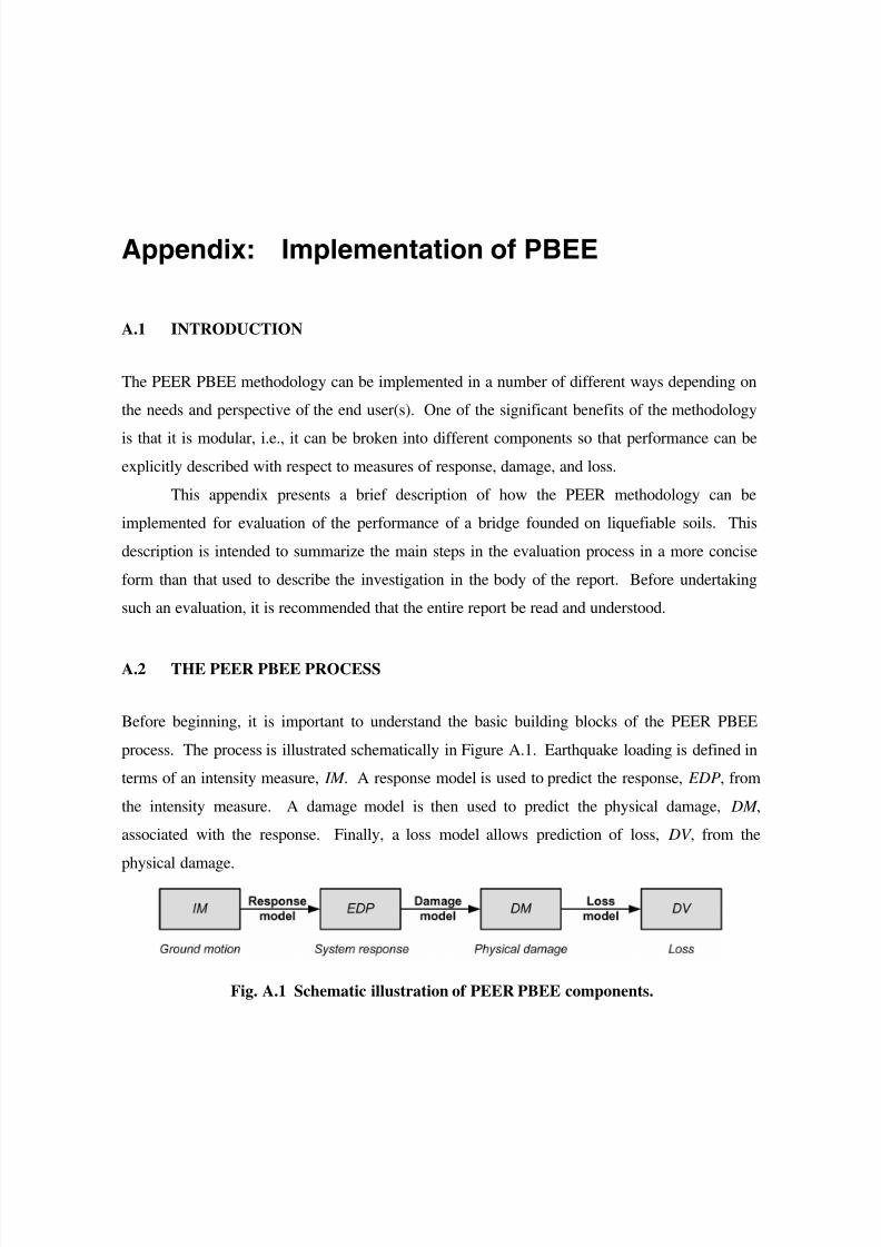
7/21/2019 PEER807 KRAMERArduino Shin
http://slidepdf.com/reader/full/peer807-kramerarduino-shin 184/198
A-1
Appendix: Implementation of PBEE
A.1 INTRODUCTION
The PEER PBEE methodology can be implemented in a number of different ways depending on
the needs and perspective of the end user(s). One of the significant benefits of the methodologyis that it is modular, i.e., it can be broken into different components so that performance can be
explicitly described with respect to measures of response, damage, and loss.
This appendix presents a brief description of how the PEER methodology can be
implemented for evaluation of the performance of a bridge founded on liquefiable soils. This
description is intended to summarize the main steps in the evaluation process in a more concise
form than that used to describe the investigation in the body of the report. Before undertaking
such an evaluation, it is recommended that the entire report be read and understood.
A.2 THE PEER PBEE PROCESS
Before beginning, it is important to understand the basic building blocks of the PEER PBEE
process. The process is illustrated schematically in Figure A.1. Earthquake loading is defined in
terms of an intensity measure, IM . A response model is used to predict the response, EDP, from
the intensity measure. A damage model is then used to predict the physical damage, DM ,
associated with the response. Finally, a loss model allows prediction of loss, DV , from the
physical damage.
Fig. A.1 Schematic illustration of PEER PBEE components.
7/21/2019 PEER807 KRAMERArduino Shin
http://slidepdf.com/reader/full/peer807-kramerarduino-shin 185/198
A-2
The intensity measure varies with exposure time in a manner commonly described by a
seismic hazard curve, which is the result of a probabilistic seismic hazard analysis. In the PEER
PBEE framework, the response is integrated (Eq. 2.1) over all values of the intensity measure—
this means that the response of the system of interest must be computed for ground motions
ranging from very weak (which may induce only elastic response) to very strong (which may
induce highly nonlinear, inelastic response). The damage measure is integrated over all levels of
response, so the selected damage model must be capable of predicting damage from both very
low and very high levels of response. Finally, the decision variable is integrated over all levels
of damage, so the loss model must predict losses from damage levels ranging from very low to
very high.
The results of the response, damage, and loss models can be represented by fragility
curves when each is expressed by a continuous random variable. This is the most common form
of output for response models, but current damage and loss models are often expressed in
discrete form; in such cases, their results can be expressed in terms of damage and loss
probability matrices.
A.3 THE PROCEDURE
The remainder of this appendix provides a concise description of the major steps in a PEERframework-based PBEE evaluation of an existing structure. The structure used to illustrate the
procedure is the bridge studied in this investigation, but the basic principles can be applied to any
structure.
1. Look at the big picture. Determine the purpose of the seismic evaluation and how the
results will be used to make retrofit, replacement, or other decisions. Identify the basis
on which such decisions will be made, i.e., define the decision variables. For illustration
procedures, this appendix will assume that decisions will be made on the basis of direct
economic losses, but other factors such as casualties, downtime, and indirect losses may
also factor into the decision process.
2. Define potential other variables of interest. Based on the decision variable(s), identify
potential damage measures (DMs). The damage measures should be those that the
decision variables are most closely related to. Identification of these variables may be
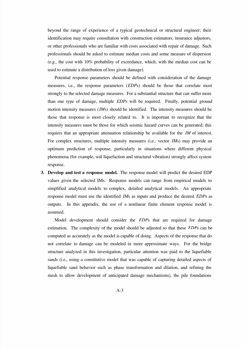
7/21/2019 PEER807 KRAMERArduino Shin
http://slidepdf.com/reader/full/peer807-kramerarduino-shin 186/198
A-3
beyond the range of experience of a typical geotechnical or structural engineer; their
identification may require consultation with construction estimators, insurance adjustors,
or other professionals who are familiar with costs associated with repair of damage. Such
professionals should be asked to estimate median costs and some measure of dispersion
(e.g., the cost with 10% probability of exceedance, which, with the median cost can be
used to estimate a distribution of loss given damage).
Potential response parameters should be defined with consideration of the damage
measures, i.e., the response parameters ( EDPs) should be those that correlate most
strongly to the selected damage measures. For a substantial structure that can suffer more
than one type of damage, multiple EDPs will be required. Finally, potential ground
motion intensity measures ( IM s) should be identified. The intensity measures should be
those that response is most closely related to. It is important to recognize that the
intensity measures must be those for which seismic hazard curves can be generated; this
requires that an appropriate attenuation relationship be available for the IM of interest.
For complex structures, multiple intensity measures (i.e., vector IM s) may provide an
optimum prediction of response, particularly in situations where different physical
phenomena (for example, soil liquefaction and structural vibration) strongly affect system
response.
3. Develop and test a response model. The response model will predict the desired EDP
values given the selected IMs. Response models can range from empirical models to
simplified analytical models to complex, detailed analytical models. An appropriate
response model must use the identified IM s as inputs and produce the desired EDPs as
outputs. In this appendix, the use of a nonlinear finite element response model is
assumed.
Model development should consider the EDPs that are required for damage
estimation. The complexity of the model should be adjusted so that these EDPs can be
computed as accurately as the model is capable of doing. Aspects of the response that do
not correlate to damage can be modeled in more approximate ways. For the bridge
structure analyzed in this investigation, particular attention was paid to the liquefiable
sands (i.e., using a constitutive model that was capable of capturing detailed aspects of
liquefiable sand behavior such as phase transformation and dilation, and refining the
mesh to allow development of anticipated damage mechanisms), the pile foundations
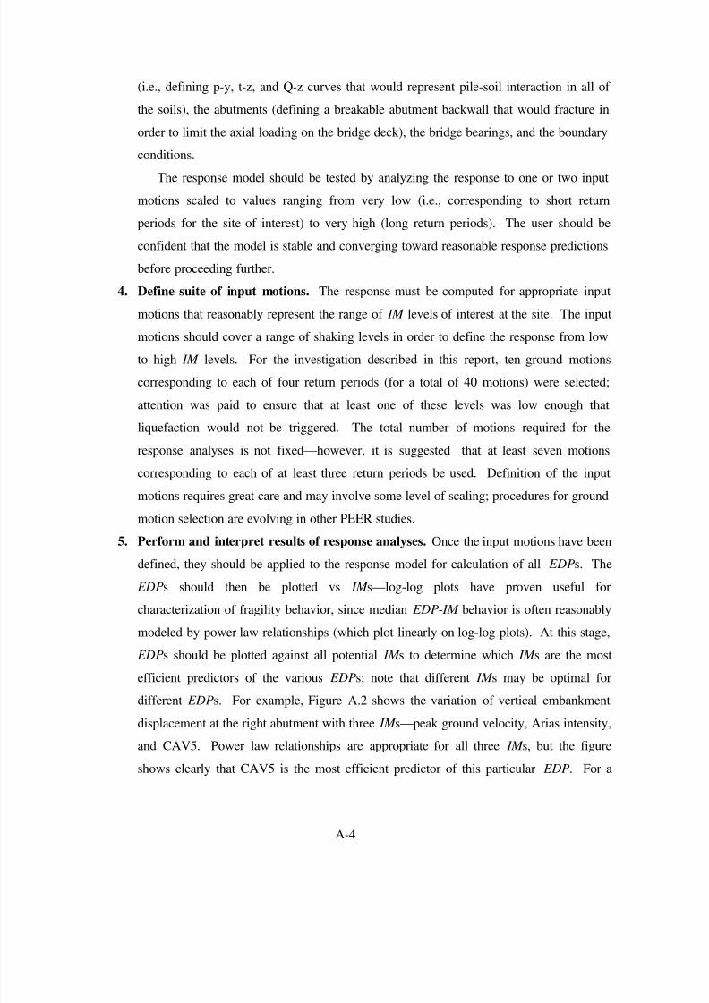
7/21/2019 PEER807 KRAMERArduino Shin
http://slidepdf.com/reader/full/peer807-kramerarduino-shin 187/198
A-4
(i.e., defining p-y, t-z, and Q-z curves that would represent pile-soil interaction in all of
the soils), the abutments (defining a breakable abutment backwall that would fracture in
order to limit the axial loading on the bridge deck), the bridge bearings, and the boundary
conditions.
The response model should be tested by analyzing the response to one or two input
motions scaled to values ranging from very low (i.e., corresponding to short return
periods for the site of interest) to very high (long return periods). The user should be
confident that the model is stable and converging toward reasonable response predictions
before proceeding further.
4. Define suite of input motions. The response must be computed for appropriate input
motions that reasonably represent the range of IM levels of interest at the site. The input
motions should cover a range of shaking levels in order to define the response from low
to high IM levels. For the investigation described in this report, ten ground motions
corresponding to each of four return periods (for a total of 40 motions) were selected;
attention was paid to ensure that at least one of these levels was low enough that
liquefaction would not be triggered. The total number of motions required for the
response analyses is not fixed—however, it is suggested that at least seven motions
corresponding to each of at least three return periods be used. Definition of the input
motions requires great care and may involve some level of scaling; procedures for ground
motion selection are evolving in other PEER studies.
5. Perform and interpret results of response analyses. Once the input motions have been
defined, they should be applied to the response model for calculation of all EDPs. The
EDPs should then be plotted vs IM s—log-log plots have proven useful for
characterization of fragility behavior, since median EDP- IM behavior is often reasonably
modeled by power law relationships (which plot linearly on log-log plots). At this stage,
EDPs should be plotted against all potential IM s to determine which IM s are the most
efficient predictors of the various EDPs; note that different IM s may be optimal for
different EDPs. For example, Figure A.2 shows the variation of vertical embankment
displacement at the right abutment with three IM s—peak ground velocity, Arias intensity,
and CAV5. Power law relationships are appropriate for all three IM s, but the figure
shows clearly that CAV5 is the most efficient predictor of this particular EDP. For a
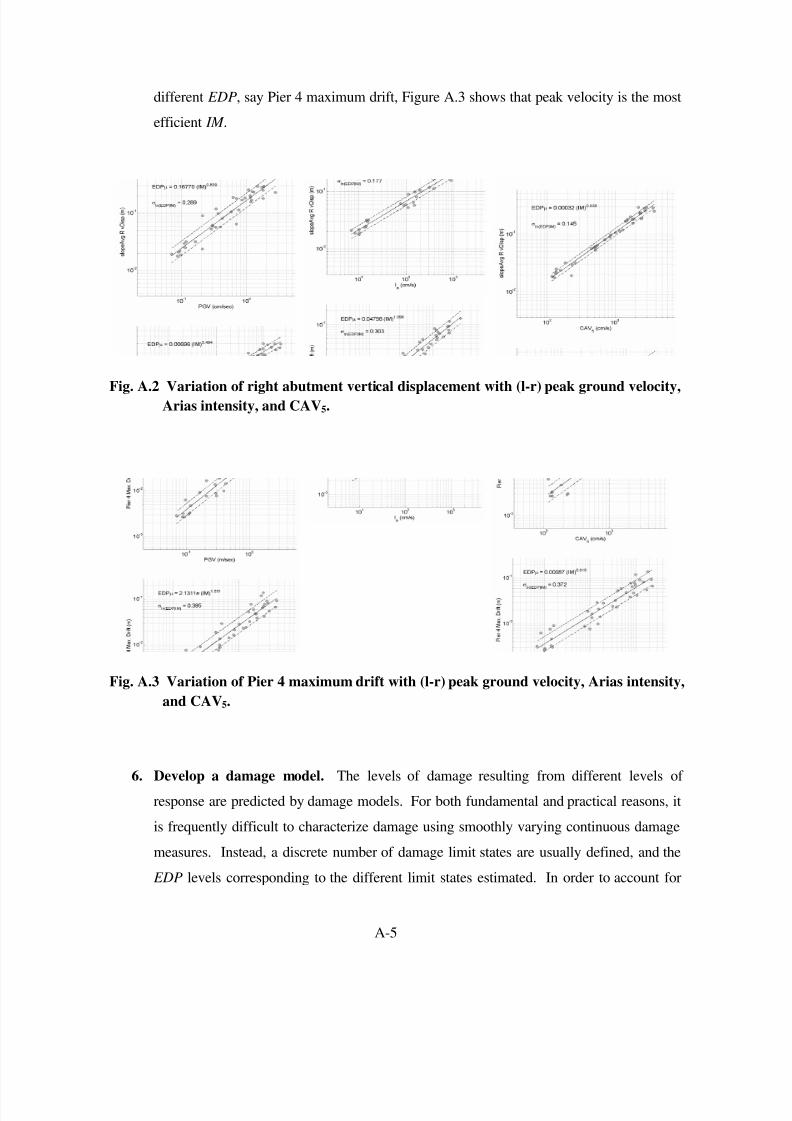
7/21/2019 PEER807 KRAMERArduino Shin
http://slidepdf.com/reader/full/peer807-kramerarduino-shin 188/198
A-5
different EDP, say Pier 4 maximum drift, Figure A.3 shows that peak velocity is the most
efficient IM .
Fig. A.2 Variation of right abutment vertical displacement with (l-r) peak ground velocity,
Arias intensity, and CAV5.
Fig. A.3 Variation of Pier 4 maximum drift with (l-r) peak ground velocity, Arias intensity,
and CAV5.
6. Develop a damage model. The levels of damage resulting from different levels of
response are predicted by damage models. For both fundamental and practical reasons, it
is frequently difficult to characterize damage using smoothly varying continuous damage
measures. Instead, a discrete number of damage limit states are usually defined, and the
EDP levels corresponding to the different limit states estimated. In order to account for
7/21/2019 PEER807 KRAMERArduino Shin
http://slidepdf.com/reader/full/peer807-kramerarduino-shin 189/198
A-6
uncertainties in capacities (i.e., the response levels corresponding to the different damage
limit states), defining a damage model generally involves estimating the median EDP
level and dispersion values at the boundaries between different limit states.
7. Develop a loss model. The losses associated with different damage limit states arepredicted by loss models. Loss models can be broken down into components associated
with different repair methods. It should be noted that loss models may not be continuous
and may not increase monotonically; for example, the cost of repairing cracks in a
column by epoxy injection will drop to zero if the damage becomes so severe that a
different repair method (or even column replacement) becomes more cost-effective.
The uncertainties associated with response, damage, and loss modeling have
generally been found to be low relative to the uncertainty in ground motions. As a result,
it may be convenient to collapse, or condense, the response, damage, and loss models into
a single model that describes loss given ground motion, i.e., DV | IM . This condensation
would take the form
∑∑ ×=>=>==> ]|(]|[]|[ jk k lil edp EDPdm DM Pdm DM dv DV Pim IM dv DV P
]|[ ik im IM edp EDPP =>(A.1)
This function actually describes a fragility surface, i.e., exceedance probabilities as a
function of both IM and DV . Graphically, the fragility surface is shown in Figure A.4. It
should be noted that the fragility curves are continuous and smooth in the DV dimension
due to the assumption of lognormally distributed losses, but irregular in the IM direction
due to the type of variability discussed in the preceding step.
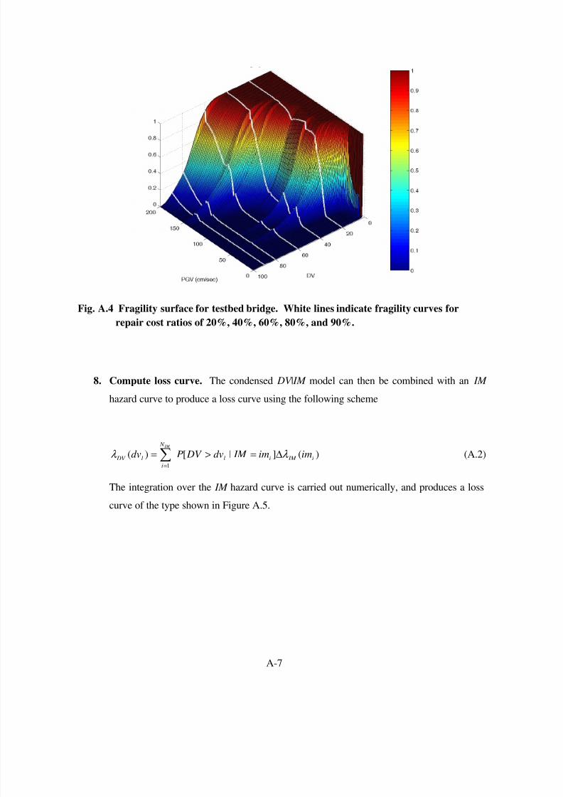
7/21/2019 PEER807 KRAMERArduino Shin
http://slidepdf.com/reader/full/peer807-kramerarduino-shin 190/198
A-7
Fig. A.4 Fragility surface for testbed bridge. White lines indicate fragility curves for
repair cost ratios of 20%, 40%, 60%, 80%, and 90%.
8. Compute loss curve. The condensed DV | IM model can then be combined with an IM
hazard curve to produce a loss curve using the following scheme
)(]|[)(1
i IM il
N
i
l DV imim IM dv DV Pdv IM
λ λ ∆=>=∑=
(A.2)
The integration over the IM hazard curve is carried out numerically, and produces a loss
curve of the type shown in Figure A.5.
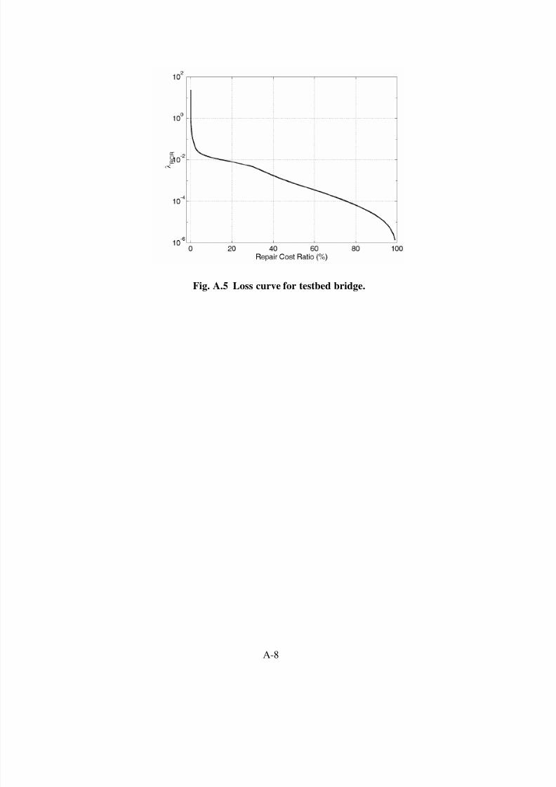
7/21/2019 PEER807 KRAMERArduino Shin
http://slidepdf.com/reader/full/peer807-kramerarduino-shin 191/198
A-8
Fig. A.5 Loss curve for testbed bridge.

7/21/2019 PEER807 KRAMERArduino Shin
http://slidepdf.com/reader/full/peer807-kramerarduino-shin 192/198
PEER REPORTS
PEER reports are available from the National Information Service for Earthquake Engineering (NISEE). To order PEER reports,please contact the Pacific Earthquake Engineering Research Center, 1301 South 46
th Street, Richmond, California 94804-4698.
Tel.: (510) 665-3405; Fax: (510) 665-3420.
PEER 2008/07 Using OpenSees for Performance-Based Evaluation of Bridges on Liquefiable Soils. Stephen L. Kramer, PedroArduino, and HyungSuk Shin. November 2008.
PEER 2008/06 Shaking Table Tests and Numerical Investigation of Self-Centering Reinforced Concrete Bridge Columns. HyungIL Jeong, Junichi Sakai, and Stephen A. Mahin. September 2008.
PEER 2008/05 Performance-Based Earthquake Engineering Design Evaluation Procedure for Bridge Foundations UndergoingLiquefaction-Induced Lateral Ground Displacement. Christian A. Ledezma and Jonathan D. Bray. August 2008.
PEER 2008/04 Benchmarking of Nonlinear Geotechnical Ground Response Analysis Procedures. Jonathan P. Stewart, AnnieOn-Lei Kwok, Yousseff M. A. Hashash, Neven Matasovic, Robert Pyke, Zhiliang Wang, and Zhaohui Yang.August 2008.
PEER 2008/03 Guidelines for Nonlinear Analysis of Bridge Structures in California. Ady Aviram, Kevin R. Mackie, and BožidarStojadinović . August 2008.
PEER 2008/02 Treatment of Uncertainties in Seismic-Risk Analysis of Transportation Systems. Evangelos Stergiou and Anne S.
Kiremidjian. July 2008.PEER 2008/01 Seismic Performance Objectives for Tall Buildings. William T. Holmes, Charles Kircher, William Petak, and Nabih
Youssef. August 2008.
PEER 2007/12 An Assessment to Benchmark the Seismic Performance of a Code-Conforming Reinforced Concrete Moment- Frame Building. Curt Haselton, Christine A. Goulet, Judith Mitrani-Reiser, James L. Beck, Gregory G. Deierlein,Keith A. Porter, Jonathan P. Stewart, and Ertugrul Taciroglu. August 2008.
PEER 2007/11 Bar Buckling in Reinforced Concrete Bridge Columns. Wayne A. Brown, Dawn E. Lehman, and John F. Stanton.February 2008.
PEER 2007/10 Computational Modeling of Progressive Collapse in Reinforced Concrete Frame Structures. Mohamed M. Talaatand Khalid M. Mosalam. May 2008.
PEER 2007/09 Integrated Probabilistic Performance-Based Evaluation of Benchmark Reinforced Concrete Bridges. Kevin R.Mackie, John-Michael Wong, and Božidar Stojadinović . January 2008.
PEER 2007/08 Assessing Seismic Collapse Safety of Modern Reinforced Concrete Moment-Frame Buildings. Curt B. Haseltonand Gregory G. Deierlein. February 2008.
PEER 2007/07 Performance Modeling Strategies for Modern Reinforced Concrete Bridge Columns. Michael P. Berry and MarcO. Eberhard. April 2008.
PEER 2007/06 Development of Improved Procedures for Seismic Design of Buried and Partially Buried Structures. Linda Al Atikand Nicholas Sitar. June 2007.
PEER 2007/05 Uncertainty and Correlation in Seismic Risk Assessment of Transportation Systems. Renee G. Lee and Anne S.Kiremidjian. July 2007.
PEER 2007/04 Numerical Models for Analysis and Performance-Based Design of Shallow Foundations Subjected to SeismicLoading. Sivapalan Gajan, Tara C. Hutchinson, Bruce L. Kutter, Prishati Raychowdhury, José A. Ugalde, andJonathan P. Stewart. May 2008.
PEER 2007/03 Beam-Column Element Model Calibrated for Predicting Flexural Response Leading to Global Collapse of RCFrame Buildings. Curt B. Haselton, Abbie B. Liel, Sarah Taylor Lange, and Gregory g. Deierlein. May 2008.
PEER 2007/02 Campbell-Bozorgnia NGA Ground Motion Relations for the Geometric Mean Horizontal Component of Peak andSpectral Ground Motion Parameters. Kenneth W. Campbell and Yousef Bozorgnia. May 2007.
PEER 2007/01 Boore-Atkinson NGA Ground Motion Relations for the Geometric Mean Horizontal Component of Peak andSpectral Ground Motion Parameters. David M. Boore and Gail M. Atkinson. May. May 2007.
PEER 2006/12 Societal Implications of Performance-Based Earthquake Engineering. Peter J. May. May 2007.
PEER 2006/11 Probabilistic Seismic Demand Analysis Using Advanced Ground Motion Intensity Measures, AttenuationRelationships, and Near-Fault Effects. Polsak Tothong and C. Allin Cornell. March 2007.
PEER 2006/10 Application of the PEER PBEE Methodology to the I-880 Viaduct. Sashi Kunnath. February 2007.

7/21/2019 PEER807 KRAMERArduino Shin
http://slidepdf.com/reader/full/peer807-kramerarduino-shin 193/198
PEER 2006/09 Quantifying Economic Losses from Travel Forgone Following a Large Metropolitan Earthquake. James Moore,Sungbin Cho, Yue Yue Fan, and Stuart Werner. November 2006.
PEER 2006/08 Vector - Valued Ground Motion Intensity Measures for Probabilistic Seismic Demand Analysis . Jack W. Baker andC. Allin Cornell. October 2006.
PEER 2006/07 Analytical Modeling of Reinforced Concrete Walls for Predicting Flexural and Coupled–Shear-Flexural Responses . Kutay Orakcal, Leonardo M. Massone, and John W. Wallace. October 2006.
PEER 2006/06 Nonlinear Analysis of a Soil-Drilled Pier System under Static and Dynamic Axial Loading. Gang Wang andNicholas Sitar. November 2006.
PEER 2006/05 Advanced Seismic Assessment Guidelines. Paolo Bazzurro, C. Allin Cornell, Charles Menun, Maziar Motahari,and Nicolas Luco. September 2006.
PEER 2006/04 Probabilistic Seismic Evaluation of Reinforced Concrete Structural Components and Systems. Tae Hyung Leeand Khalid M. Mosalam. August 2006.
PEER 2006/03 Performance of Lifelines Subjected to Lateral Spreading. Scott A. Ashford and Teerawut Juirnarongrit. July 2006.
PEER 2006/02 Pacific Earthquake Engineering Research Center Highway Demonstration Project. Anne Kiremidjian, JamesMoore, Yue Yue Fan, Nesrin Basoz, Ozgur Yazali, and Meredith Williams. April 2006.
PEER 2006/01 Bracing Berkeley. A Guide to Seismic Safety on the UC Berkeley Campus. Mary C. Comerio, Stephen Tobriner,and Ariane Fehrenkamp. January 2006.
PEER 2005/16Seismic Response and Reliability of Electrical Substation Equipment and Systems. Junho Song, Armen DerKiureghian, and Jerome L. Sackman. April 2006.
PEER 2005/15 CPT-Based Probabilistic Assessment of Seismic Soil Liquefaction Initiation. R. E. S. Moss, R. B. Seed, R. E.Kayen, J. P. Stewart, and A. Der Kiureghian. April 2006.
PEER 2005/14 Workshop on Modeling of Nonlinear Cyclic Load-Deformation Behavior of Shallow Foundations. Bruce L. Kutter,Geoffrey Martin, Tara Hutchinson, Chad Harden, Sivapalan Gajan, and Justin Phalen. March 2006.
PEER 2005/13 Stochastic Characterization and Decision Bases under Time-Dependent Aftershock Risk in Performance-BasedEarthquake Engineering. Gee Liek Yeo and C. Allin Cornell. July 2005.
PEER 2005/12 PEER Testbed Study on a Laboratory Building: Exercising Seismic Performance Assessment. Mary C. Comerio,editor. November 2005.
PEER 2005/11 Van Nuys Hotel Building Testbed Report: Exercising Seismic Performance Assessment. Helmut Krawinkler,editor. October 2005.
PEER 2005/10 First NEES/E-Defense Workshop on Collapse Simulation of Reinforced Concrete Building Structures. September2005.
PEER 2005/09 Test Applications of Advanced Seismic Assessment Guidelines. Joe Maffei, Karl Telleen, Danya Mohr, WilliamHolmes, and Yuki Nakayama. August 2006.
PEER 2005/08 Damage Accumulation in Lightly Confined Reinforced Concrete Bridge Columns. R. Tyler Ranf, Jared M. Nelson,Zach Price, Marc O. Eberhard, and John F. Stanton. April 2006.
PEER 2005/07 Experimental and Analytical Studies on the Seismic Response of Freestanding and Anchored LaboratoryEquipment. Dimitrios Konstantinidis and Nicos Makris. January 2005.
PEER 2005/06 Global Collapse of Frame Structures under Seismic Excitations . Luis F. Ibarra and Helmut Krawinkler.September 2005.
PEER 2005//05 Performance Characterization of Bench- and Shelf-Mounted Equipment. Samit Ray Chaudhuri and Tara C.Hutchinson. May 2006.
PEER 2005/04 Numerical Modeling of the Nonlinear Cyclic Response of Shallow Foundations. Chad Harden, Tara Hutchinson,Geoffrey R. Martin, and Bruce L. Kutter. August 2005.
PEER 2005/03 A Taxonomy of Building Components for Performance-Based Earthquake Engineering. Keith A. Porter.September 2005.
PEER 2005/02 Fragility Basis for California Highway Overpass Bridge Seismic Decision Making . Kevin R. Mackie and BožidarStojadinović . June 2005.
PEER 2005/01 Empirical Characterization of Site Conditions on Strong Ground Motion. Jonathan P. Stewart, Yoojoong Choi,and Robert W. Graves. June 2005.
PEER 2004/09 Electrical Substation Equipment Interaction: Experimental Rigid Conductor Studies. Christopher Stearns andAndré Filiatrault. February 2005.

7/21/2019 PEER807 KRAMERArduino Shin
http://slidepdf.com/reader/full/peer807-kramerarduino-shin 194/198
PEER 2004/08 Seismic Qualification and Fragility Testing of Line Break 550-kV Disconnect Switches. Shakhzod M. Takhirov,Gregory L. Fenves, and Eric Fujisaki. January 2005.
PEER 2004/07 Ground Motions for Earthquake Simulator Qualification of Electrical Substation Equipment. Shakhzod M.Takhirov, Gregory L. Fenves, Eric Fujisaki, and Don Clyde. January 2005.
PEER 2004/06 Performance-Based Regulation and Regulatory Regimes. Peter J. May and Chris Koski. September 2004.
PEER 2004/05 Performance-Based Seismic Design Concepts and Implementation: Proceedings of an International Workshop.
Peter Fajfar and Helmut Krawinkler, editors. September 2004.
PEER 2004/04 Seismic Performance of an Instrumented Tilt-up Wall Building. James C. Anderson and Vitelmo V. Bertero. July2004.
PEER 2004/03 Evaluation and Application of Concrete Tilt-up Assessment Methodologies. Timothy Graf and James O. Malley.October 2004.
PEER 2004/02 Analytical Investigations of New Methods for Reducing Residual Displacements of Reinforced Concrete BridgeColumns. Junichi Sakai and Stephen A. Mahin. August 2004.
PEER 2004/01 Seismic Performance of Masonry Buildings and Design Implications. Kerri Anne Taeko Tokoro, James C.Anderson, and Vitelmo V. Bertero. February 2004.
PEER 2003/18 Performance Models for Flexural Damage in Reinforced Concrete Columns. Michael Berry and Marc Eberhard.August 2003.
PEER 2003/17 Predicting Earthquake Damage in Older Reinforced Concrete Beam-Column Joints. Catherine Pagni and LauraLowes. October 2004.
PEER 2003/16 Seismic Demands for Performance-Based Design of Bridges. Kevin Mackie and Božidar Stojadinović
. August2003.
PEER 2003/15 Seismic Demands for Nondeteriorating Frame Structures and Their Dependence on Ground Motions. RicardoAntonio Medina and Helmut Krawinkler. May 2004.
PEER 2003/14 Finite Element Reliability and Sensitivity Methods for Performance-Based Earthquake Engineering. TerjeHaukaas and Armen Der Kiureghian. April 2004.
PEER 2003/13 Effects of Connection Hysteretic Degradation on the Seismic Behavior of Steel Moment-Resisting Frames. JaniseE. Rodgers and Stephen A. Mahin. March 2004.
PEER 2003/12 Implementation Manual for the Seismic Protection of Laboratory Contents: Format and Case Studies. William T.Holmes and Mary C. Comerio. October 2003.
PEER 2003/11 Fifth U.S.-Japan Workshop on Performance-Based Earthquake Engineering Methodology for ReinforcedConcrete Building Structures. February 2004.
PEER 2003/10 A Beam-Column Joint Model for Simulating the Earthquake Response of Reinforced Concrete Frames. Laura N.Lowes, Nilanjan Mitra, and Arash Altoontash. February 2004.
PEER 2003/09 Sequencing Repairs after an Earthquake: An Economic Approach. Marco Casari and Simon J. Wilkie. April 2004.
PEER 2003/08 A Technical Framework for Probability-Based Demand and Capacity Factor Design (DCFD) Seismic Formats .Fatemeh Jalayer and C. Allin Cornell. November 2003.
PEER 2003/07 Uncertainty Specification and Propagation for Loss Estimation Using FOSM Methods. Jack W. Baker and C. AllinCornell. September 2003.
PEER 2003/06 Performance of Circular Reinforced Concrete Bridge Columns under Bidirectional Earthquake Loading . MahmoudM. Hachem, Stephen A. Mahin, and Jack P. Moehle. February 2003.
PEER 2003/05 Response Assessment for Building-Specific Loss Estimation. Eduardo Miranda and Shahram Taghavi.
September 2003.
PEER 2003/04 Experimental Assessment of Columns with Short Lap Splices Subjected to Cyclic Loads . Murat Melek, John W.Wallace, and Joel Conte. April 2003.
PEER 2003/03 Probabilistic Response Assessment for Building-Specific Loss Estimation. Eduardo Miranda and HesameddinAslani. September 2003.
PEER 2003/02 Software Framework for Collaborative Development of Nonlinear Dynamic Analysis Program. Jun Peng andKincho H. Law. September 2003.
PEER 2003/01 Shake Table Tests and Analytical Studies on the Gravity Load Collapse of Reinforced Concrete Frames. KennethJohn Elwood and Jack P. Moehle. November 2003.

7/21/2019 PEER807 KRAMERArduino Shin
http://slidepdf.com/reader/full/peer807-kramerarduino-shin 195/198
PEER 2002/24 Performance of Beam to Column Bridge Joints Subjected to a Large Velocity Pulse. Natalie Gibson, AndréFiliatrault, and Scott A. Ashford. April 2002.
PEER 2002/23 Effects of Large Velocity Pulses on Reinforced Concrete Bridge Columns. Greg L. Orozco and Scott A. Ashford.April 2002.
PEER 2002/22 Characterization of Large Velocity Pulses for Laboratory Testing. Kenneth E. Cox and Scott A. Ashford. April2002.
PEER 2002/21 Fourth U.S.-Japan Workshop on Performance-Based Earthquake Engineering Methodology for ReinforcedConcrete Building Structures . December 2002.
PEER 2002/20 Barriers to Adoption and Implementation of PBEE Innovations. Peter J. May. August 2002.
PEER 2002/19 Economic-Engineered Integrated Models for Earthquakes: Socioeconomic Impacts. Peter Gordon, James E.Moore II, and Harry W. Richardson. July 2002.
PEER 2002/18 Assessment of Reinforced Concrete Building Exterior Joints with Substandard Details. Chris P. Pantelides, JonHansen, Justin Nadauld, and Lawrence D. Reaveley. May 2002.
PEER 2002/17 Structural Characterization and Seismic Response Analysis of a Highway Overcrossing Equipped withElastomeric Bearings and Fluid Dampers: A Case Study. Nicos Makris and Jian Zhang. November 2002.
PEER 2002/16 Estimation of Uncertainty in Geotechnical Properties for Performance-Based Earthquake Engineering. Allen L.Jones, Steven L. Kramer, and Pedro Arduino. December 2002.
PEER 2002/15Seismic Behavior of Bridge Columns Subjected to Various Loading Patterns. Asadollah Esmaeily-Gh. and YanXiao. December 2002.
PEER 2002/14 Inelastic Seismic Response of Extended Pile Shaft Supported Bridge Structures. T.C. Hutchinson, R.W.Boulanger, Y.H. Chai, and I.M. Idriss. December 2002.
PEER 2002/13 Probabilistic Models and Fragility Estimates for Bridge Components and Systems. Paolo Gardoni, Armen DerKiureghian, and Khalid M. Mosalam. June 2002.
PEER 2002/12 Effects of Fault Dip and Slip Rake on Near-Source Ground Motions: Why Chi-Chi Was a Relatively Mild M7.6Earthquake. Brad T. Aagaard, John F. Hall, and Thomas H. Heaton. December 2002.
PEER 2002/11 Analytical and Experimental Study of Fiber-Reinforced Strip Isolators . James M. Kelly and Shakhzod M. Takhirov.September 2002.
PEER 2002/10 Centrifuge Modeling of Settlement and Lateral Spreading with Comparisons to Numerical Analyses . SivapalanGajan and Bruce L. Kutter. January 2003.
PEER 2002/09 Documentation and Analysis of Field Case Histories of Seismic Compression during the 1994 Northridge,California, Earthquake. Jonathan P. Stewart, Patrick M. Smith, Daniel H. Whang, and Jonathan D. Bray. October2002.
PEER 2002/08 Component Testing, Stability Analysis and Characterization of Buckling-Restrained Unbonded Braces TM
. CameronBlack, Nicos Makris, and Ian Aiken. September 2002.
PEER 2002/07 Seismic Performance of Pile-Wharf Connections. Charles W. Roeder, Robert Graff, Jennifer Soderstrom, and JunHan Yoo. December 2001.
PEER 2002/06 The Use of Benefit-Cost Analysis for Evaluation of Performance-Based Earthquake Engineering Decisions .Richard O. Zerbe and Anthony Falit-Baiamonte. September 2001.
PEER 2002/05 Guidelines, Specifications, and Seismic Performance Characterization of Nonstructural Building Components andEquipment . André Filiatrault, Constantin Christopoulos, and Christopher Stearns. September 2001.
PEER 2002/04 Consortium of Organizations for Strong-Motion Observation Systems and the Pacific Earthquake EngineeringResearch Center Lifelines Program: Invited Workshop on Archiving and Web Dissemination of GeotechnicalData, 4–5 October 2001. September 2002.
PEER 2002/03 Investigation of Sensitivity of Building Loss Estimates to Major Uncertain Variables for the Van Nuys Testbed. Keith A. Porter, James L. Beck, and Rustem V. Shaikhutdinov. August 2002.
PEER 2002/02 The Third U.S.-Japan Workshop on Performance-Based Earthquake Engineering Methodology for ReinforcedConcrete Building Structures . July 2002.
PEER 2002/01 Nonstructural Loss Estimation: The UC Berkeley Case Study. Mary C. Comerio and John C. Stallmeyer. December 2001.
PEER 2001/16 Statistics of SDF-System Estimate of Roof Displacement for Pushover Analysis of Buildings. Anil K. Chopra,Rakesh K. Goel, and Chatpan Chintanapakdee. December 2001.

7/21/2019 PEER807 KRAMERArduino Shin
http://slidepdf.com/reader/full/peer807-kramerarduino-shin 196/198
PEER 2001/15 Damage to Bridges during the 2001 Nisqually Earthquake. R. Tyler Ranf, Marc O. Eberhard, and Michael P.Berry. November 2001.
PEER 2001/14 Rocking Response of Equipment Anchored to a Base Foundation. Nicos Makris and Cameron J. Black.September 2001.
PEER 2001/13 Modeling Soil Liquefaction Hazards for Performance-Based Earthquake Engineering. Steven L. Kramer andAhmed-W. Elgamal. February 2001.
PEER 2001/12 Development of Geotechnical Capabilities in OpenSees. Boris Jeremi . September 2001.
PEER 2001/11 Analytical and Experimental Study of Fiber-Reinforced Elastomeric Isolators . James M. Kelly and Shakhzod M.Takhirov. September 2001.
PEER 2001/10 Amplification Factors for Spectral Acceleration in Active Regions. Jonathan P. Stewart, Andrew H. Liu, YoojoongChoi, and Mehmet B. Baturay. December 2001.
PEER 2001/09 Ground Motion Evaluation Procedures for Performance-Based Design. Jonathan P. Stewart, Shyh-Jeng Chiou,Jonathan D. Bray, Robert W. Graves, Paul G. Somerville, and Norman A. Abrahamson. September 2001.
PEER 2001/08 Experimental and Computational Evaluation of Reinforced Concrete Bridge Beam-Column Connections forSeismic Performance . Clay J. Naito, Jack P. Moehle, and Khalid M. Mosalam. November 2001.
PEER 2001/07 The Rocking Spectrum and the Shortcomings of Design Guidelines. Nicos Makris and Dimitrios Konstantinidis.August 2001.
PEER 2001/06Development of an Electrical Substation Equipment Performance Database for Evaluation of EquipmentFragilities . Thalia Agnanos. April 1999.
PEER 2001/05 Stiffness Analysis of Fiber-Reinforced Elastomeric Isolators. Hsiang-Chuan Tsai and James M. Kelly. May 2001.
PEER 2001/04 Organizational and Societal Considerations for Performance-Based Earthquake Engineering. Peter J. May. April2001.
PEER 2001/03 A Modal Pushover Analysis Procedure to Estimate Seismic Demands for Buildings: Theory and PreliminaryEvaluation. Anil K. Chopra and Rakesh K. Goel. January 2001.
PEER 2001/02 Seismic Response Analysis of Highway Overcrossings Including Soil-Structure Interaction. Jian Zhang and NicosMakris. March 2001.
PEER 2001/01 Experimental Study of Large Seismic Steel Beam-to-Column Connections. Egor P. Popov and Shakhzod M.Takhirov. November 2000.
PEER 2000/10 The Second U.S.-Japan Workshop on Performance-Based Earthquake Engineering Methodology for Reinforced
Concrete Building Structures. March 2000.
PEER 2000/09 Structural Engineering Reconnaissance of the August 17, 1999 Earthquake: Kocaeli (Izmit), Turkey. Halil Sezen,Kenneth J. Elwood, Andrew S. Whittaker, Khalid Mosalam, John J. Wallace, and John F. Stanton. December2000.
PEER 2000/08 Behavior of Reinforced Concrete Bridge Columns Having Varying Aspect Ratios and Varying Lengths ofConfinement. Anthony J. Calderone, Dawn E. Lehman, and Jack P. Moehle. January 2001.
PEER 2000/07 Cover-Plate and Flange-Plate Reinforced Steel Moment-Resisting Connections. Taejin Kim, Andrew S. Whittaker,Amir S. Gilani, Vitelmo V. Bertero, and Shakhzod M. Takhirov. September 2000.
PEER 2000/06 Seismic Evaluation and Analysis of 230-kV Disconnect Switches. Amir S. J. Gilani, Andrew S. Whittaker, GregoryL. Fenves, Chun-Hao Chen, Henry Ho, and Eric Fujisaki. July 2000.
PEER 2000/05 Performance-Based Evaluation of Exterior Reinforced Concrete Building Joints for Seismic Excitation. ChandraClyde, Chris P. Pantelides, and Lawrence D. Reaveley. July 2000.
PEER 2000/04 An Evaluation of Seismic Energy Demand: An Attenuation Approach. Chung-Che Chou and Chia-Ming Uang. July1999.
PEER 2000/03 Framing Earthquake Retrofitting Decisions: The Case of Hillside Homes in Los Angeles. Detlof von Winterfeldt,Nels Roselund, and Alicia Kitsuse. March 2000.
PEER 2000/02 U .S.-Japan Workshop on the Effects of Near-Field Earthquake Shaking. Andrew Whittaker, ed. July 2000.
PEER 2000/01 Further Studies on Seismic Interaction in Interconnected Electrical Substation Equipment. Armen Der Kiureghian,Kee-Jeung Hong, and Jerome L. Sackman. November 1999.
PEER 1999/14 Seismic Evaluation and Retrofit of 230 -kV Porcelain Transformer Bushings . Amir S. Gilani, Andrew S. Whittaker,Gregory L. Fenves, and Eric Fujisaki. December 1999.

7/21/2019 PEER807 KRAMERArduino Shin
http://slidepdf.com/reader/full/peer807-kramerarduino-shin 197/198
PEER 1999/13 Building Vulnerability Studies: Modeling and Evaluation of Tilt-up and Steel Reinforced Concrete Buildings. JohnW. Wallace, Jonathan P. Stewart, and Andrew S. Whittaker, editors. December 1999.
PEER 1999/12 Rehabilitation of Nonductile RC Frame Building Using Encasement Plates and Energy-Dissipating Devices. Mehrdad Sasani, Vitelmo V. Bertero, James C. Anderson. December 1999.
PEER 1999/11 Performance Evaluation Database for Concrete Bridge Components and Systems under Simulated SeismicLoads. Yael D. Hose and Frieder Seible. November 1999.
PEER 1999/10 U.S.-Japan Workshop on Performance-Based Earthquake Engineering Methodology for Reinforced ConcreteBuilding Structures. December 1999.
PEER 1999/09 Performance Improvement of Long Period Building Structures Subjected to Severe Pulse-Type Ground Motions .James C. Anderson, Vitelmo V. Bertero, and Raul Bertero. October 1999.
PEER 1999/08 Envelopes for Seismic Response Vectors. Charles Menun and Armen Der Kiureghian. July 1999.
PEER 1999/07 Documentation of Strengths and Weaknesses of Current Computer Analysis Methods for Seismic Performance ofReinforced Concrete Members. William F. Cofer. November 1999.
PEER 1999/06 Rocking Response and Overturning of Anchored Equipment under Seismic Excitations. Nicos Makris and JianZhang. November 1999.
PEER 1999/05 Seismic Evaluation of 550 kV Porcelain Transformer Bushings. Amir S. Gilani, Andrew S. Whittaker, Gregory L.Fenves, and Eric Fujisaki. October 1999.
PEER 1999/04Adoption and Enforcement of Earthquake Risk-Reduction Measures.
Peter J. May, Raymond J. Burby, T. JensFeeley, and Robert Wood.
PEER 1999/03 Task 3 Characterization of Site Response General Site Categories . Adrian Rodriguez-Marek, Jonathan D. Bray,and Norman Abrahamson. February 1999.
PEER 1999/02 Capacity-Demand-Diagram Methods for Estimating Seismic Deformation of Inelastic Structures: SDF Systems .Anil K. Chopra and Rakesh Goel. April 1999.
PEER 1999/01 Interaction in Interconnected Electrical Substation Equipment Subjected to Earthquake Ground Motions. ArmenDer Kiureghian, Jerome L. Sackman, and Kee-Jeung Hong. February 1999.
PEER 1998/08 Behavior and Failure Analysis of a Multiple-Frame Highway Bridge in the 1994 Northridge Earthquake. Gregory L.Fenves and Michael Ellery. December 1998.
PEER 1998/07 Empirical Evaluation of Inertial Soil-Structure Interaction Effects. Jonathan P. Stewart, Raymond B. Seed, andGregory L. Fenves. November 1998.
PEER 1998/06 Effect of Damping Mechanisms on the Response of Seismic Isolated Structures. Nicos Makris and Shih-PoChang. November 1998.
PEER 1998/05 Rocking Response and Overturning of Equipment under Horizontal Pulse-Type Motions. Nicos Makris andYiannis Roussos. October 1998.
PEER 1998/04 Pacific Earthquake Engineering Research Invitational Workshop Proceedings, May 14–15, 1998: Defining theLinks between Planning, Policy Analysis, Economics and Earthquake Engineering. Mary Comerio and PeterGordon. September 1998.
PEER 1998/03 Repair/Upgrade Procedures for Welded Beam to Column Connections. James C. Anderson and Xiaojing Duan.May 1998.
PEER 1998/02 Seismic Evaluation of 196 kV Porcelain Transformer Bushings. Amir S. Gilani, Juan W. Chavez, Gregory L.Fenves, and Andrew S. Whittaker. May 1998.
PEER 1998/01 Seismic Performance of Well-Confined Concrete Bridge Columns. Dawn E. Lehman and Jack P. Moehle.December 2000.

7/21/2019 PEER807 KRAMERArduino Shin
http://slidepdf.com/reader/full/peer807-kramerarduino-shin 198/198
ONLINE REPORTS
The following PEER reports are available by Internet only at http://peer.berkeley.edu/publications/peer_reports.html
PEER 2008/101 Seismic Performance Objectives for Tall Buildings. William T. Holmes, Charles Kircher, William Petak, and NabihYoussef. August 2008.
PEER 2007/101 Generalized Hybrid Simulation Framework for Structural Systems Subjected to Seismic Loading. Tarek Elkhoraibiand Khalid M. Mosalam. July 2007.
PEER 2007/100 Seismic Evaluation of Reinforced Concrete Buildings Including Effects of Masonry Infill Walls. Alidad Hashemiand Khalid M. Mosalam. July 2007.