UNIVERSITY OF QUEBEC AT CHICOUTIMI

MANUSCRIPT-BASED THESIS PRESENTED TO

UNIVERSITY OF QUEBEC AT CHICOUTIMI

IN PARTIAL FULFILLMENT OF THE REQUIREMENTS FOR THE DEGREE OF

PHILOSOPHIAE DOCTOR

Ph.D.

IN EARTH AND ATMOSPHERIC SCIENCES

OFFERED AT

UNIVERSITY OF QUEBEC AT MONTREAL

UNDER A MEMORANDUM OF UNDERSTANDING

WITH THE UNIVERSITY OF QUEBEC AT CHICOUTIMI

BY

FAYÇAL LAMRAOUI

IN-CLOUD ICING AND SUPERCOOLED CLOUD MICROPHYSICS:

FROM REANALYSIS TO MESOSCALE MODELING

NOVEMBER 2014

© Fayçal Lamraoui, 2014

The ice storm - January 1998

Oil on canvas painting – Artist: A. Poirier

In the distance, the Montérégie, viewed from Mont-Royal (Montreal, Quebec, Canada)

(Courtesy of the community Ste-Croix, Saint-Laurent)

iii

ABSTRACT

In-cloud icing is continually associated with potential hazardous meteorological

conditions at higher altitudes in the troposphere across the world and near surface over

mountainous and cold climate regions. This PhD thesis aims to scrutinize the horizontal and

vertical characteristics of near-surface in-cloud icing events, the associated cloud

microphysics, develop and demonstrate an innovative method to determine the climatology

of icing events at high resolution. In reference to ice accretion, the quantification of icing

events is based on the cylinder model. With the use of North American Regional

Reanalysis, a preliminary mapping of the icing severity index spanning a 32-year time

period is introduced and in that way the freezing precipitation during the ice storm of

January 1998 is quantified and compared to observations. Also, case studies over Mount-

Bélair and Bagotville are investigated. The assessment of icing events obtained from

NARR demonstrates agreements with observation over simple terrains and disparities over

complex terrains, due to the coarse resolution of the reanalysis. Subsequently, three-

dimensional high resolution climatology of in-cloud icing is produced within the

atmospheric layer between 10 and 200 m above ground. Upgraded method utilizes a new

hybrid approach that merges the insignificant icing days obtained from NARR with the

significant icing days obtained from high resolution double-nested modeling down to a

resolution of 5 km. The findings reveal the vertical profile of icing events and demonstrate

an improvement in capturing them over complex terrains. The results indicate typical

supercooled cloud droplets around 15 μm, the corresponding typical temperatures ranging

from -15 to 0 °C and the critical altitudes of 60 and 100 m above ground that trigger the

accentuation of the icing severity.

Particular attention is given to the impact of the icing events on the production of

wind energy, in order to introduce an original weighting factor that reflects power

degradation due to the icing events. This potential weighting can serve to obtain a more

personalized icing severity index for wind turbines under icing conditions. The additional

power loss factor is based on an analogy between the blades of a wind turbine and a sub-

iv

scaled helicopter. The critical freezing fraction 0.88 of supercooled droplets associated with

the double horn ice shape is found to occupy a restricted segment on the blade and

gradually moves towards the tip with decreasing temperature. Substantial power

degradation of wind turbines with supercooled liquid water contents 0.04 g·m−3

, 0.07

g·m−3

, 0.2 g·m−3

, and 0.36 g·m−3

occurs at temperatures T=-2.6 °C, -4.5 °C, -12 °C, and -20

°C respectively.

Keywords: Atmospheric icing, Reanalysis, Mesoscale modeling, Cloud microphysics,

Near-surface climate.

v

RÉSUMÉ

Le givrage dans les nuages est constamment associé à des conditions météorologiques

potentiellement dangereuses à des altitudes plus élevées dans la troposphère à travers le

monde et près de la surface dans les régions montagneuses et du climat froid. Cette thèse de

doctorat vise à examiner les caractéristiques horizontales et verticales des événements de

givrage dans les nuages près de la surface, la microphysique des nuages associée,

développer et démontrer une méthode innovante pour déterminer la climatologie des

événements de givrage à haute résolution. Concernant l'accumulation de la glace, la

quantification du givrage dans les nuages est fondée sur le modèle de cylindre. Avec

l'utilisation des réanalyses régionales nord-américaines (NARR), une cartographie

préliminaire de l'indice de sévérité du givrage dans les nuages couvrant une période de 32

ans est présentée. La tempête de verglas de janvier 1998 est quantifiée et comparée aux

observations. Études de cas sur le Mont-bélair et l’aéroport de Bagotville sont étudiés.

L'évaluation des événements de givrage obtenus à partir NARR démontre des accords avec

l'observation sur les terrains simples et des disparités sur les terrains complexes, en raison

de la faible résolution des réanalyses NARR. Par la suite, une climatologie

tridimensionnelle de givrage à haute résolution est produite dans la couche atmosphérique

entre 10 et 200 m au-dessus du sol. La méthode améliorée utilise une nouvelle approche

hybride qui fusionne les jours de givrage insignifiant obtenus à partir NARR avec les jours

de givrage significatif obtenus à partir une cascade de deux niveaux imbriqués de

modélisation méso-échelle jusqu'à une résolution de 5 km. Les résultats révèlent le profil

vertical des événements de givrage et démontrent une amélioration dans la détection de ces

événements sur les terrains complexes. Les résultats indiquent des valeurs typiques de

gouttelettes nuageuses en surfusion autour 15 μm, les températures typiques

correspondantes varient de -15 jusqu'à 0°C et les altitudes critiques de 60 et 100 m au-

dessus du sol qui marquent le déclenchement de l'accentuation de la sévérité du givrage

dans les nuages.

vi

Une attention particulière est accordée à l'impact des événements de givrage sur la

production de l'énergie éolienne, afin d'introduire un facteur de pondération originale qui

reflète la dégradation de puissance due à des événements de givrage. Cette pondération

potentielle peut servir à personnaliser l'indice de sévérité pour les éoliennes dans des

conditions de givrage. Le facteur additionnel de perte de puissance est fondé sur une

analogie entre les pales d'une éolienne et un hélicoptère. La fraction de congélation critique

0,88 de gouttelettes en surfusion qui est associée à la forme double-horn de glace se trouve

à occuper un segment restreint sur la pale et se déplace vers le bout lorsque la température

diminue progressivement. Les dégradations substantielles de puissance des éoliennes qui

correspondent aux teneurs en eau liquide surfondue 0.04 g·m−3

, 0.07 g·m−3

, 0.2 g·m−3

, et

0.36 g·m−3

se produisent à des températures T=-2.6 °C, -4.5 °C, -12 °C, et -20 °C

respectivement.

Mots-clés: Givrage atmosphérique, Réanalyse, Modélisation méso-échelle, Microphysique

des nuages, Climatologie près de la surface.

vii

ACKNOWLEDGEMENTS

I Firstly, I would like to thank my supervisor Professor Jean Perron for his financial support

throughout my thesis and for his valuable contribution to this project. He made certain that

all was at my disposal in order to ensure the progress of my Ph.D. thesis.

I also want to thank my co-director Professor Robert Benoit, who guided me throughout

this entire process. I am grateful he shared with me his experience and valuable art of

numerical modeling, especially with GEM-LAM and MC2.

I want to extend my thanks to Dr. Guy Fortin from Bombardier Aerospace for his

significant contribution during this thesis, particularly his willingness to share his

knowledge of wind turbines and aviation under icing conditions.

I want to express my deep gratitude to the jury members who participated in my

dissertation, for their interest and for accepting and evaluating my thesis. I thank the

external member, Dr. Anna Glazer from Environment Canada and also Professor Jean-

Louis Laforte from AMIL-UQAC for carefully reviewing my PhD thesis. Their invaluable

suggestions and comments have enriched this dissertation.

I also thank Professor Christian Masson for his contribution to my research project and for

welcoming me in his laboratory "The Research Laboratory on the Nordic Environment

Aerodynamics of Wind Turbines (NEAT)" and allowing me access to all its facilities.

I want to extend my thanks to Dr. Jason Milbrandt from Environment Canada for his

availability and the time he took with me to help clarify several aspects of his cloud

microphysics scheme which is used with the mesoscale model GEM-LAM in this project.

Many thanks to my colleagues Amélie Camion for her contribution toward the GRIB-RPN

format converter, Dr. Nicolas Gasset for the time he took to help, particularly at the

beginning of my thesis, to adapt with the available version of both models MC2, GEM and

the use of the cluster, as well as Dr. Alex Flores-Maradiaga for our discussions and

comparisons regarding the performances of the Models MC2, GEM-LAM and WRF.

I also thank Professor Michael Higgins and Agathe Tremblay as well as the team of AMIL-

UQAC, namely Elizabeth Crook, Caroline Blackburn and particularly Dr.Caroline Laforte

for providing the icing events measurements of Hydro-Quebec and Environment Canada

over the sites of the Mount Belair and the Airport of Bagotville respectively.

viii

My affectionate gratitude goes to my dear mother Aïcha "Beboul" and my father Youcef

"Bechikh", exemplary parents in my eyes, who taught me to overlook all obstacles. My

father, who wants all his children to become doctors, can now be proud of this third

doctoral degree achieved by another of his children. I thank my sister Wahida and my

brothers Fethi and Nabil as well. I want to extend a special thanks to my parents-in-law

Maria and Domenico for always lending a helpful hand whenever it was needed.

Finally, I would like to express, my deepest gratitude to my wife Maria Teresa who has

always been by my side and supportive throughout the process of my PhD. I dedicate this

work to my family and especially my wife and my two children, who have given me a new

life full of joy and love.

TABLE OF CONTENTS

ABSTRACT .......................................................................................................................... iii

RÉSUMÉ ................................................................................................................................ v ACKNOWLEDGEMENTS ..................................................................................................vii TABLE OF CONTENTS ....................................................................................................... ix LIST OF FIGURES ..............................................................................................................xii LIST OF ACRONYMS ....................................................................................................... xiv

LIST OF SYMBOLS ............................................................................................................ xv INTRODUCTION .................................................................................................................. 1

In-cloud icing ...................................................................................................................... 3 Cloud physics and ice accretion ...................................................................................... 3

Topography and icing events .......................................................................................... 3

Challenges and motivations ................................................................................................ 5 Hazard assessment of icing events .................................................................................. 5

Mesoscale Modeling of Atmospheric icing .................................................................... 6

Objective ............................................................................................................................. 8

Structure of the thesis ......................................................................................................... 9

References ......................................................................................................................... 11

CHAPTER 1 ......................................................................................................................... 15 1. ATMOSPHERIC ICING SEVERITY: QUANTIFICATION AND MAPPING ......... 16

Abstract ............................................................................................................................. 16 1.1 Introduction ............................................................................................................ 17 1.2 Methodology .......................................................................................................... 22

1.2.1 Reanalysis Data ............................................................................................... 24

1.2.2 Icing calculations ............................................................................................ 25

1.2.3 Icing events ..................................................................................................... 28

1.2.4 Freezing rain storm of 1998 ............................................................................ 28

1.2.5 Icing severity index ......................................................................................... 31

1.3 Results .................................................................................................................... 33 1.3.1 Case studies ..................................................................................................... 34

1.3.2 Ice storm of January 1998 ............................................................................... 44

1.3.3 Icing severity index ......................................................................................... 48

1.4 Discussion of the results......................................................................................... 55

1.5 Conclusion.............................................................................................................. 58 1.6 References .............................................................................................................. 60

CHAPTER 2 ......................................................................................................................... 65 2. HYBRID FINE SCALE CLIMATOLOGY AND MICROPHYSICS OF IN-CLOUD

ICING: FROM 32KM REANALYSIS TO 5KM MESOSCALE MODELING .................. 66

x

Abstract ............................................................................................................................. 66 2.1 Introduction ............................................................................................................ 67 2.2 Method ................................................................................................................... 70

2.3 Results .................................................................................................................... 73 2.3.1 Climatology of atmospheric icing ................................................................... 73

2.3.2 Transition from 32-year to 15-year ................................................................. 75

2.3.3 GEM-LAM and NARR performances ............................................................ 78

2.3.4 Selection of significant days ........................................................................... 81

2.3.5 Mesoscale modeling and simulation setup ..................................................... 83

2.3.6 Statistics and cloud microphysics properties .................................................. 87

2.3.7 Vertical profile of icing events climatology ................................................... 89

2.3.8 Icing severity index at fine scale resolution .................................................... 93

2.4 Conclusion............................................................................................................ 100 2.5 References ............................................................................................................ 102

CHAPTER 3 ....................................................................................................................... 106 3. ATMOSPHERIC ICING IMPACT ON WIND TURBINE PRODUCTION ............ 107

Abstract ........................................................................................................................... 107

3.1 Introduction .......................................................................................................... 108

3.2 Methodology ........................................................................................................ 112 3.2.1 Generic wind turbine .................................................................................... 113

3.2.2 Blade ............................................................................................................. 113

3.2.3 Chord ............................................................................................................ 113

3.2.4 Airfoil ............................................................................................................ 114

3.2.5 Speed ............................................................................................................. 115

3.3 Ice accretion model .............................................................................................. 116

3.4 Power distribution model ..................................................................................... 117 3.5 Results .................................................................................................................. 119

3.5.1 Power along the blade ................................................................................... 119

3.5.2 Water collection effeciency .......................................................................... 120

3.5.3 Ice mass rate .................................................................................................. 121

3.5.4 Aerodynamic effect ....................................................................................... 122

3.5.5 Freezing fraction ........................................................................................... 125

3.5.6 Power loss ..................................................................................................... 128

3.6 Analysis ................................................................................................................ 138

3.7 Conclusion............................................................................................................ 142 3.8 References ............................................................................................................ 144

GENERAL CONCLUSION ............................................................................................... 147

xi

LIST OF TABLES

TABLE 1.1 : SEVERITY CLASSES ............................................................................................................... 32 TABLE 1.2 : MONTHLY KEY VARIABLE IN THE TWO SITES ............................................................... 35 TABLE 2.1 : SELECTED SIGNIFICANT DAYS FOR GEM-LAM .............................................................. 82 TABLE 2.2 : GRID SETUP FOR THE NUMERICAL EXPERIMENT ......................................................... 84 TABLE 2.3 : THE LOWEST 17 VERTICAL LEVELS USED IN GEM-LAM THAT CORRESPOND TO

ABL ......................................................................................................................................................... 84 TABLE 3.1 : DURATION OF ICING EVENTS FROM REANALYSIS: 32-YEAR ICING CLIMATE ..... 135

LIST OF FIGURES

FIGURE 1.1. A HYDRO-QUEBEC ICING-RATE METER (AMIL-UQAC). ............................................... 24 FIGURE 1.2. LIQUID WATER CONTENT CALCULATED USING PRECIPITATION RATE FROM

REANALYSIS THAT COVERS THE PERIOD JANUARY 04TH UNTIL JANUARY 10TH. .......... 30 FIGURE 1.3. MEDIAN VOLUME DIAMETER CALCULATED USING PRECIPITATION RATE FROM

REANALYSIS THAT COVERS THE PERIOD JANUARY 04TH UNTIL JANUARY 10TH. .......... 30 FIGURE 1.4. CROSS-SECTION OF NARR TOPOGRAPHY. ...................................................................... 34 FIGURE 1.5. MONTHLY MODEL-BASED CALCULATION AND MEASUREMENTS ON

BAGOTVILLE; ...................................................................................................................................... 37 FIGURE 1.6. MONTHLY MODEL-BASED CALCULATION AND MEASUREMENTS ON MT BÉLAIR;

(A) DURATION OF ICING EVENTS (B) ACCUMULATION OF ICE. ............................................. 39 FIGURE 1.7. CLIMATOLOGY OF MODEL-BASED IN-CLOUD ICING EVENTS, DURATION AND

ACCUMULATION OVER BAGOTVILLE IN JANUARY FOR 32 YEARS. ..................................... 40 FIGURE 1.8. MODEL-BASED MONTHLY DURATION OF ICING EVENTS IN JANUARY FOR 32

YEARS AT MOUNT BÉLAIR (QUEBEC, CANADA). ....................................................................... 41 FIGURE 1.9. MONTHLY MODEL-BASED SEVERITY AND ICE ACCUMULATION ON

BAGOTVILLE DURING JANUARY OF EACH YEAR - 32 YEARS. ................................................ 43 FIGURE 1.10. MONTHLY MODEL-BASED SEVERITY AND ICE ACCUMULATION ON MT BÉLAIR

DURING JANUARY OF EACH YEAR - 32 YEARS. .......................................................................... 43 FIGURE 1.11. ICING ACCUMULATION FROM JANUARY 4 TO 10, 1998 OVER THE

SOUTHWESTERN REGION OF QUEBEC (CANADA) (A) ICE ACCUMULATION

CALCULATED USING NARR REANALYSIS ................................................................................... 47 FIGURE 1.12 : ICING SEVERITY INDEX MAP - JANUARY 1979–2010. ................................................. 49 FIGURE 1.13. ICING SEVERITY INDEX MAP - FEBRUARY 1979–2010. ............................................... 50 FIGURE 1.14. ICING SEVERITY INDEX MAP - DECEMBER 1979–2010. ............................................... 51 FIGURE 1.15. ICING SEVERITY INDEX MAP — 3 MONTH'S AVERAGE 1979–2010........................... 54 FIGURE 2.1. HYBRID APPROACH USING NARR 32KM AND GEM-LAM 5KM COMBINATION. ..... 71 FIGURE 2.2. MEAN VALUES OF THE ICE ACCUMULATION AND THE DURATION OF ICING

EVENTS (JANUARY: 1980-2009) ........................................................................................................ 74 FIGURE 2.3. COMPARISON BETWEEN THE ICING SEVERITY INDEX DURING 32 YEARS AND 15

YEARS OVER 17 X 20 NARR CELLS CENTRED AT RIVIERE-DU-LOUP .................................... 76 FIGURE 2.4. COMPARISON BETWEEN 32 YEARS AND 15 YEARS: DURATION OF ICING EVENTS

(A,B), ICE ACCUMULATION (C,D) AND ICING SEVERITY INDEX (E,F). COLOUR SCALES

ARE CLIPPED FOR THE 15 YEAR PERIOD. ..................................................................................... 77 FIGURE 2.5. TOPOGRAPHY CROSS SECTION VIEWED BY NARR 32KM, GEM-LAM 5KM AND

GEM-LAM 1KM .................................................................................................................................... 79 FIGURE 2.6. COMPARISON OF TEMPERATURES FROM NARR 32 KM, GEM-LAM 5KM AND

OBSERVATION ..................................................................................................................................... 80 FIGURE 2.7. COMPARISON OF ISI OVER MOUNT-BELAIR (15 YEARS) WITH ALL DAYS VERSUS

SELECTED DAYS. ................................................................................................................................ 82 FIGURE 2.8. SIMULATION DOMAINS AND TARGET ZONE .................................................................. 86 FIGURE 2.9. STATISTICS OF METEOROLOGICAL ICING PARAMETERS ........................................... 88 FIGURE 2.10. VERTICAL PROFILES OF HIGH RESOLUTION 15-YEAR CLIMATOLOGY OF ICING

EVENTS: (A) SEVERITY CLASSES (B) DURATION OF ICING EVENTS (C) ICE

ACCUMULATION (D) TOPOGRAPHY FROM GEM-LAM5KM ...................................................... 91 FIGURE 2.11. 15-YEAR CLIMATOLOGY OF ICING SEVERITY INDEX AT 1000 MB: (A) NARR 32

KM, (B) GEM-LAM 5KM ...................................................................................................................... 94 FIGURE 2.12. 15-YEAR CLIMATOLOGY OF ICE ACCUMULATION AND DURATION OF ICING

EVENTS AT 40M, 80M AND 120 ......................................................................................................... 96 FIGURE 2.13. VERTICAL PROFILES OF ICE ACCUMULATION AND DURATION OF ICING EVENTS

BETWEEN 10 AND 200 M. ................................................................................................................... 98

xiii

FIGURE 2.14. 15-YEAR CLIMATOLOGY OF ICING SEVERITY INDEX AT 80 M. ............................... 99 FIGURE 3.1. CHORD VARIATION ALONG THE SPAN ......................................................................... 114 FIGURE 3.2. NACA 63-415 AIRFOIL .......................................................................................................... 115 FIGURE 3.3. ELEMENTARY SPAN OF WIND TURBINE ....................................................................... 117 FIGURE 3.4. ELEMENTARY POWER COEFFICIENT ALONG THE SPAN ........................................... 119 FIGURE 3.5. COLLECTION EFFICIENCY ALONG THE BLADE FOR DIFFERENT DROPLET

DIAMETERS (FOG, DRIZZLE, RAIN) .............................................................................................. 121 FIGURE 3.6. ICE MASS RATE ALONG THE SPAN FOR DIFFERENT LIQUID WATER CONTENTS.

............................................................................................................................................................... 122 FIGURE 3.7. MAXIMUM ICE THICKNESS RATE ALONG THE SPAN FOR DIFFERENT LIQUID

WATER CONTENT ............................................................................................................................. 123 FIGURE 3.8. AERODYNAMIC EFFECT ALONG THE BLADE FOR LWC =0.2 G∙M

-3. ......................... 124

FIGURE 3.9. LUDLAM LIMIT FOR DIFFERENT LIQUID WATER CONTENT.................................... 126 FIGURE 3.10. FREEZING FRACTION ALONG THE SPAN FOR DIFFERENT TEMPERATURES (LWC

= 0.2 G·M−3

). ......................................................................................................................................... 127 FIGURE 3.11. AERODYNAMIC REDUCTION FACTOR (A) POWER LOSS VS FREEZING FRACTION

(B) POWER LOSS VS TEMPERATURE FOR DIFFERENT LIQUID WATER CONTENTS. ........ 130 FIGURE 3.12. POWER LOSS AT R/R ~ [0.93 0.96] FOR DIFFERENT LIQUID WATER CONTENTS. 132 FIGURE 3.13. REQUIRED DURATION FOR ICE ACCRETION ON WIND TURBINES TO MATCH

THE SAME HIGHEST POWER LOSS UNDER ICING CONDITIONS ON HELICOPTER'S

BLADES (FREEZING FRACTION 0.88, R/R= [0.93 0.96]) FOR DIFFERENT LIQUID WATER

CONTENTS. ......................................................................................................................................... 134 FIGURE 3.14. MONTHLY DURATION OF ICING EVENTS FROM REANALYSIS OVER MOUNT-

BÉLAIR SITE DURING JANUARY (FROM 1979 TO 2010). ........................................................... 135 FIGURE 3.15. POWER UNDER ICING EFFECTS FOR LWC = 0.2 G · M−3 AT T = −12 °C AND T =

−13.5 °C, (A) POWER CURVE WITH AND WITHOUT ICING (B) ELECTRICAL POWER LOSS.

............................................................................................................................................................... 137

xiv

LIST OF ACRONYMS

AGL Above Ground Level

AMIL Anti-icing Material International Laboratory

CCN Cloud condensation nuclei

CMC Canadian Meteorological Center

DM Double Moment

DJF December January February

FAA Federal Aviation Administration

FST CMC/RPN standard file

GEM-LAM Global Environment Multiscale Limited Area Model

GRIB GRIdded Binary

IRM Icing Rate Meter

M&Y Milbrandt and Yau

NACA National Advisory Committee for Aeronautics

NARR North American Regional Reanalysis

NCAR National Center for Atmospheric Research

NCEP National Center for Environmental Prediction

NOAA National Oceanic and Atmospheric Administration

NWP Numerical Weather Prediction

PGSM Programme Général de Sortie des Modèles de RPN

RPN Recherche en Prévision Numérique

RTD Resistance Temperature Detector

SGE Sun Grid Engine

SLD Supercooled Large Droplets

3DVAR Three-dimensional Variational Data Assimilation

xv

LIST OF SYMBOLS

A Accumulation parameter

c Chord [m]

CLWMR Cloud liquid water mixing ratio [kg·kg-1

]

Power Coefficient for clean blade

Power Coefficient for iced blade

dc Cylinder diameter [m]

dx grid spacing [m]

Ice thickness rate [mm·hr-1

]

E Total collection efficiency

F Freezing fraction

Power loss factor

h Ice accumulation [mm]

h Ice accumulation [mm]

Ice thickness rate [mm·hr-1

]

ISI Icing severity index [mm]

IWC Ice water content [g·m-3

]

LWC Liquid water content [g·m-3

]

λ Tip speed ratio

Mass rate of liquid water per unit surface [g·m-2

·s-1

]

MVD Median volume diameter [μm]

μa Dynamic viscosity of air [Pa·s]

Ω Rotational speed [RPM]

R Length of the blade [m]

r Radial position [m]

Ice density [kg·m-3

]

Water density [kg·m-3

]

SLWC Supercooled liquid water content [g·m-3

]

xvi

St Stokes number

SW Monthly icing index [mm]

T Temperature [°K]

t0 Time for starting simulation [hr]

TCWC Total cloud water content [g·m-3

]

The duration for ice accretion on helicopter [hr]

TMP Temperature [°K]

The duration for ice accretion on wind turbine [hr]

U Wind speed [m∙s-1

]

UGRD Zonal wind speed [m·s-1

]

VGRD Meridional wind speed [m·s-1

]

WL Weighting for liquid water content

Wt Weighting for icing event duration

x Position along the span [m]

INTRODUCTION

The increasing awareness with respect to preserving the environment has emerged

after realizing the substantial level of damages caused by mishandling of nature. Over the

last several decades research continues for safer ways to provide cleaner energy. The

renewable energy market in Canada is expanding rapidly, due in large part to increased

demand for energy sources that are environmentally preferable to, and more secure than,

fossil fuels. In addition to the conscious effort, the increasing cost and the continuous

depletion of fossil fuels have prompted the transition to clean energies that are abundant.

Canadian utility companies have begun to diversify their energy portfolio by investing in

the development of wind energy and other renewable energy sources. Despite a great

potential of wind energy, the considerable technical barriers that affect wind energy

systems operating in the Canadian climate and geography have so far hindered their

widespread deployment in Canada. Weather related energy sources are subject to the

variability of atmospheric conditions that can be reinforcing or problematic. Therefore,

weather intelligence that accurately provides details about the present and the future

atmospheric behaviors is required for a safe and profitable extraction of clean energy. Hau

(2013) reported that onshore wind power is among the most cost-effective clean energy. On

the other hand, this eco-friendly alternative is exposed to challenging near-surface icing

conditions. These hazardous events will therfore affect automatically the power industry

(Bernstein et al., 2011).

2

At high altitudes in the troposphere in-cloud icing is the dominant atmospheric

condition that imposes economic challenges and safety concerns to aircraft navigation

around the globe. On the other hand, at lower atmospheric levels near the surface, only the

mountainous and cold climate regions are frequently exposed to icing events that can

endanger near-surface structures, including wind turbines and power lines. Atmospheric

icing issues have been studied from two points of view; by analyzing the meteorological

conditions (cloud physics and cloud dynamics) which lead to icing events and from a

mechanical perspective (adherence, accretion, icephobic materials…).

The direct meteorological key parameters : liquid water content, cloud droplets size,

wind speed and temperature, control the quantification of in-cloud icing. These parameters

do not contribute equally to the intensity of icing events. For this reason, an appropriate

assessment of the severity of the icing event requires weighting factors which reflect the

level of influence of each parameter. In addition, elevated topography with accentuated

gradient slopes contribute significantly in originating near-surface orographic clouds and

generating larger sizes of cloud droplets. Therefore, to accurately evaluate the icing events

over complex terrains, it is crucial to involve an advanced microphysics scheme and

meteorological variables at high resolution.

3

In-cloud icing

Cloud physics and ice accretion

In addition to the influential impacts of cloud on radiation and precipitations, the

presence of cloud is a prerequisite for the occurrence of in-cloud icing. Therefore, it is

crucial to understand cloud physical and dynamical mechanisms that favor icing events.

Several atmospheric lifting processes (orographic, convective, frontal) contribute in

triggering cloud formation. Within the subfreezing range of temperatures, cloud liquid

water content and the associated droplets sizes, together with the wind speed, regulate the

potential of the icing severity accordingly.

The atmospheric supercooled liquid water is the main indicator of the potential

occurrence of atmospheric icing, either in-cloud or precipitation icing (Marwitz et al.,

1997). Ice accretion on structure can be identified as glaze and rime. This type of icing

event is determined by the following meteorological variables: air temperature, wind speed,

size of supercooled water droplets and atmospheric water-content (Felin 1988).

Topography and icing events

Within the troposphere, various parameters such as temperature, moisture, air

density, solar radiation and wind speed vary according to the height above sea level

(Whiteman 2000). The effect of the topography and the position of the measuring station in

combination with the height of wind turbines do not allow for a precise estimation of wind

speed (Fortin et al 2005b) and consequently the icing events.

A mountain, depending on its size, shape, orientation, as well as the moisture of the air

mass in a given area, can affect the regional climate by acting as a barrier to the regional

4

flows. The latitude, altitude, continentality, and exposure to regional circulations provide a

general description of the climate of the mountainous region (Whiteman 2000).

Microclimate factors will not be discussed; they are not the defined focus of this

dissertation.

The concept and the classification of mountainous areas are completely arbitrary (Marsh,

2002). Neither qualitative nor quantitative distinction is established to identify the

difference between mountains and hills. In North America, it is common to consider 600

meters as a limit that distinguishes the difference between mountains and hills (Thompson

1964). The altitudinal range of 600 m is enough to alter the vertical profile of the

atmosphere (Roger 2008). Troll (1973) describes high mountains according to the features

of a given landscape and the microclimate in the present and in the past near ground level.

Bailey (1990) reported that rime ice can be expected for at least 10% of the time, during

cold weather when the altitude is at approximately 700 m. Commonly, rime ice occurs in

areas where supercooled cloud episodes often appear, especially when cloud bases are

below mountain summits, strong wind speed, and large surfaces which collect supercooled

droplets. Moreover, the latitude is an important factor that affects the climate of any given

site because of the angle of solar radiation and most importantly because of its exposure to

latitudinal belts of high and low pressure. These conditions reflect the potential significant

rime accumulation on middle latitudes and Polar Regions (Whiteman 2000).

In reference to complex terrains located in the province of Quebec (Canada), the

Mount-Bélair (485 m), located near Québec city, was selected to carry out ice accretion

experiments. The topography of the Mount Bélair site as well as its proximity to the St-

5

Lawrence river makes it a prime location for the formation of atmospheric icing (Hardy et

al., 1998). Similarly, the Mount Valin (980 m) in the Saguenay region is considered an

ideal location for ice accretion (Savadjiev et al., 1996, Druez et al., 1988).

Challenges and motivations

Hazard assessment of icing events

In various studies that have addressed the accretion of ice, the severity of icing

events was often assessed either by the duration of events (eg. Comeau et al., 2007), the

accumulation rate (eg. Byrkjedal and Berge, 2009) or Severity index combining key

parameters using weighting factors (eg. Lamraoui et al., 2013; Bernstein et al., 2006).

Despite the fact that icing severity is controlled mainly by the liquid water content, droplet

size and temperature (Bernstein et al., 2006), Hansman (1989) reported that the liquid water

content and temperature have a dominant contribution.

The occurrence of icing events is often associated with the concern over the

potential risk that can be generated. The assessment of the hazard level depends on weather

conditions and the vulnerability of structures that intercept supercooled water. Depending

on the field of application and the nature of structures affected by the ice, a large number of

studies have assessed the seriousness of the economic and the safety consequences that

range from perturbation to disaster. Among the structures that are vulnerable to ice

accretion are the following; aircraft (eg. Cole and Sand, 1991; Gent et al., 2000), wind

turbines (eg. Lamraoui et al., 2014; Etemaddar et al., 2014); power lines (Farzaneh 2008;

Sakamoto, 2000), meteorological instruments (Fortin et al., 2005b; Tammelin et al., 1998).

The hazardous impact of icing events on wind turbines is not exclusive to high amount of

6

ice accumulation; several studies (Marjaniemi and Peltola 1998, Jasinski, et al., 1998)

demonstrated that even modest amounts of ice accumulation on the leading edge of the

blade deteriorate substantially the aerodynamic of the blade and consequently reduce the

expected electric power. In addition, Magued et al (1989) has associated 0.055% of the

Canadian power failure to the occurrences of ice accretion on Power lines and

telecommunication towers. This rate of power outage is five times higher than reliability

level in the Canadian Design Code (CSA-S37). Moreover, in reference to tall structures

under icing conditions, there is a lack in identifying the vertical profile of icing events

(Makkonen et al., 2014). A previous experimental study that took place in Murdochville

(Quebec), confirmed that the severity of icing events depends not only on the accumulation

rate but also on the length of icing events (Fortin et al., 2005a).

Mesoscale Modeling of Atmospheric icing

In atmospheric science, the horizontal mesoscale ranges from a few kilometers to

several hundred kilometers, where the vertical scale covers all the troposphere (Pielke

2001) with a time scale that covers one hour to yearly activity. During the last two decades

the study of the microphysics of clouds has made great advances. Relative humidity is not

involved in the icing rate calculations; however it is still considered the key parameter for

icing estimations and a very good indicator for icing risk assessment. In addition to

temperature and wind speed, the droplet size distribution and the liquid water content are

the main parameters for icing. The lack of direct measurements of icing events has

motivated researchers in atmospheric icing to use analytical, empirical, or numerical

models of ice accretion as a function of meteorological variables (Makkonen, 1998 ;

7

Draganoiu et al., 1996; Jones, 1998).

Many numerical weather prediction models were used to produce an accurate forecast the

occurrences of icing events in order to match field observations. As an example of these

models, namely the ALADIN, HIRLAM, NCAR CAM, UKMO, MM5, WRF and GEM.

Vassbo et al (1998) pioneered the use of the numerical weather prediction model

(HIRLAM) to produce an atmospheric icing forecast. Drage and Hauge (2008) used the

MM5 mesoscale model to simulate atmospheric icing by employing the microphysics

scheme of Reisner (1998). Milbrandt et al (2006) have developed a sophisticated

microphysics scheme that continually evolves. This scheme was initialy created for the

Mesoscale Compressible Community Model MC2 (Benoit et al., 1997) that then was

tranfered to the model GEM which is utilized in this thesis.

The RPN/CMC (Recherche en Prévision numérique/Centre Météorologique

Canadien) Physics library is a comprehensive resource for advanced microphysics schemes;

however they are not yet fully explored and used for atmospheric icing forecasts. These

schemes provide information about icing intensity, weather hazards, such as freezing rain,

mixed precipitation, fog or blowing snow (Guan et al., 2002).

According to Anthes (1983), studies using limited area mesoscale numerical models

have considerably improved the skill of weather forecasting in general. An accurate

prediction of natural icing hazards is very important; however numerous atmospheric icing

algorithms need improvement, as is the case with the icing algorithm of Thompson

(Thompson et al., 1997) which overestimates the icing forecast. Contrary to this, the

Canadian microphysics scheme of Tremblay et al (1995) often underestimates icing events,

8

and provide a binary Yes-No forecast, without any information regarding the intensity of

icing (Tremblay and Glazer, 2000). Most freezing forecasts are based on the presence of a

warm layer. In spite of this, freezing event hydrometeors formed without a warm layer are

often observed (Strapp et al., 1996). A study focused on the central England area (model

run 3 days 7-8-9 December 1990) by Wareing and Nygaard (2009), resulted with a strong

match between measurements and accretion simulated by WRF. In this study the model

considers only the icing rate higher than 10 g∙h-1

.

Objective

This dissertation is the results of a joint collaboration between Hydro-Québec’s

research institute (IREQ), École de Technologie Supérieure and The Anti-Icing Materials

International Laboratory (AMIL) which is an engineering research laboratory associated

with the UQAC and it specializes in the certification of de/anti-icing fluids used on

airplanes before takeoff.

In general, this thesis targets all near-surface structures that are sensitive to ice

accretion and gives a particular attention to the industry of wind turbines under icing

conditions. The diversity of the cold Canadian climate and its topographic heterogeneity

impose major challenges on structure; (i) icing conditions and (ii) complex terrain.

The main objective of this dissertation focuses on the risk assessment associated with near-

surface structures under icing conditions, over simple and complex terrains. In order to

relevantly assess the hazards of icing conditions, this thesis aims to quantify the intensity of

icing events based on an original icing severity index (ISI). The ISI involves different

weighting factors that reflect the contribution of the key parameters that control the icing

9

events accordingly. In addition, this thesis gives particular attention to the occurence of

icing events and their impact on the performance of wind turbines.

This thesis aims at representing the climatology of icing events that occurred historically,

displaying averages and extreme values of parameters that describe icing events like

frequency, duration, intensity, and wind properties. To achieve this icing climatology, this

thesis uses North American Regional Reanalysis spanning a 32 year time period and a

mesoscale modeling that spans a 15 year time period.

Structure of the thesis

This thesis consists of bringing together three published peer-reviewed articles, each

of these articles represents a chapter of this dissertation and tackles one section of the

ensemble of this project. The first Chapter represents simultaneously the preliminary step

for the characterization of icing events and the primary section for the foundation of the

icing severity index that assesses the severity level of icing events. The results presented in

this chapter utilize a very large database at pressure level of 1000 mb obtained from NARR

to identify the near-surface climatology of icing events during an unprecedented long time

period of 32 years (1979-2010). The cylinder model was used to quantify icing events. For

validation purpose, comparisons were made with observation from case studies over

complex terrain, simple terrain and the ice storm 1998. The first article revealed that the use

of NARR data has a limitation regarding the detection of icing events over complex

terrains. For this reason, the second article in the second chapter intervened to improve the

resolution and implicate advanced microphyics scheme. The second article used NARR

10

data to initiate the mesoscale model GEM-LAM followed by double-nested downscaling to

obtain three-dimensional high resolution microphysics and in-cloud icing climatology.

The icing severity index (ISI) that has been addressed in chapter 1 and 2 involves

meteorological weighting factors that determine the severity level of the icing events.

Subsequently, in an effort to explore additional factors that contribute to the significance of

icing events on wind turbine production, chapter three focuses exclusively on the impact of

icing events on wind turbine production. An original power loss factor which is a potential

weighting for the icing severity index is introduced. In addition, this chapter addresses the

location and the type of the accumulated ice on the blade, the corresponding meteorological

conditions and consequently the resulting loss of wind energy.

11

References

Anthes, R. A., 1983. A review of regional models of the atmosphere in middle latitudes.

Mon. Weather Rev. 111(6), 1306-1335.

Bailey, B. H., 1990. The Potential for Icing of Wind Turbines in the Northeastern U.S.

Windpower 1990: 286-291.

Benoit, R. and Co-authors., 1997. The Canadian MC2: A Semi-Lagrangian, Semi-Implicit

Wideband Atmospheric Model Suited for Finescale. Mon. Weather Rev. 125, 2382-2415.

Bernstein, B. C. and Co-authors., 2006. The New {CIP} Icing Severity Product.Proc. of

{AMS} Conference on Aviation Range and Aerospace Meteorology.

Bernstein, B.C., Wittmeyer. I., Gregow, E. and Hirvonen, J., 2011. LAPS-LOWICE: A

real-time system for the assessment of near-surface icing conditions. Proc 14th IWAIS,

Chongqing, China, May 8 - May 13, 2011.

Byrkjedal, Ø. and Berge, E., 2009. Meso-scale models shows promising results in

predicting icing, Proc. of EWEC, Marseille, France

Cole, J., and W. R. Sand., 1991. Statistical Study of aircraft Icing Accidents. Proc. 29th

Aerospace Sciences Meeting, Reno, NV, Amer. Inst. Aero. And Astro., AIAA 91-0558.

Comeau, M. Masson, C. Morency, F. and Pelletier, F., 2007. Estimation of icing events

using NARR data. Proc 12th

IWAIS, Yokohama, Japon

Drage, M.A. and Hauge, G., 2008. Atmospheric icing in a coastal mountainous terrain.

Measurements and numerical simulations, a case study. Cold Reg. Sci. Technol, 53(2) 150-

161.

Draganoiu, G., Lamarche, L. and McComber, P., 1996. A Computer Model of Glaze

Accretion on Wires. J Offshore mech arct. 118(2), 148–157

Druez, J., M Comber, P. and Félin, B., 1988. Icing rate measurements made for different

cable configurations on an icing test line at Mt. Valin. Proc 4th IWAIS, Paris, France,

pp.477-485.

Etemaddar, M., Hansen, M.O.L. and Moan, T., 2014. Wind turbine aerodynamic response

under atmospheric icing conditions. Wind Energy, 17(2), p.241-265.

Farzaneh, M., 2008. Atmospheric Icing of Power Networks. Berlin: Springer, 381 pp

Felin, B., 1988. Freezing Rain in Quebec. Field Observations Compared to Model

Estimations. Proc 4th IWAIS, Paris. 119-123.

12

Felin, B., 1976. The observations of rime and glaze deposits in Quebec. Canadian Electrical

Association Spring Meeting, 22-24 March 1976, Toronto, 53 p

Fortin, G., Perron, J. and Ilinca., A., 2005a. A study of Icing Events at Murdochville –

Conclusions for the Wind Power Industry. Quebec Premier Wind Energy Event,

International Conference, Wind Energy Remote Regions, Magdalene Islands, Québec,

Canada

Fortin, G., Perron, J. and Ilinca A., 2005b. Behaviour and Modeling of Cup Anemometers

under Icing Conditions, Proc 11th IWAIS, Montreal, Canada, June 12-16, 2005

Gent, R. W., Dart, N. P. and Cansdale, J. T., 2000: Aircraft icing. Philos. Trans. Roy. Soc.,

358A, 2873–2911.

Guan, H., Cober, S.G., Isaac, G.A., Tremblay, A. Méthot, A., 2002. Comparison of Three

Cloud Forecast Schemes with In Situ Aircraft Measurements. Wea. Forecasting. 17, 1226-

1235.

Hansman, R.J., 1989. The influence of ice accretion physics on the forecasting of aircraft

icing conditions. Preprints, 3rd Int’l Conf. on the aviation weather system, Anaheim CA.

Hardy.C., Brunelle .J., Chevalier, J., Manoukian, B. and Vilandre, R., 1998. Telemonitoring

of climate loads on Hydro-Quebec 735 KV lines. Atmos. Res. 46(1-2), 181-191.

Hau, E., 2013. Wind turbine economics. Wind Turbines: Fundamentals, Technologies,

Application, Economics, 3rd

edition, Springer, 845-870.

Jones, K.F., 1998. A simple model for freezing rain ice loads. Atmos. Res. 46(1-2), 87–97.

Lamraoui, F., Fortin, G., Benoit, R., Perron, J. and Masson, C., 2013. Atmospheric icing

severity: Quantification and mapping. Atmos. Res. 128, 57-75.

Lamraoui, F., Fortin, G., Benoit, R., Perron, J. and Masson, C., 2014. Atmospheric icing

impact on wind turbine production. Cold Reg. Sci. Technol. 100, 36–49.

Magued, M.H., Bruneau, M. and Dryburgh, R.B., 1989. Evolution of Design Standards and

recorded Failures of Guyed Towers in Canada. Can J civil eng. 16, 725-732.

Marjaniemi, M. and Peltola, E., 1998. Blade Heating Element Design and Practical

Experiences. BOREAS IVFMI, Hetta, Finland 197–209.

Makkonen, L., 1998. Modelling power line icing in freezing precipitation. Atmos. Res.46,

131-142.

13

Makkonen, L., Lehtonen, P. and Hirviniemi, M., 2014. Determining ice loads for tower

structure design. Engineering Structures, 74, 229-232.

Marsh, J., 2002. Mountains of the world. a global priority. Environ Rev, 10(3), 191-193.

Marwitz, J., Politovich, M., Bernstein, B., Ralph, F., Neiman, P., Ashenden, R. and Bresch,

J., 1997. Meteorological conditions associated with the ATR72 aircraft accident near

Roselawn, Indiana, on 31 October 1994. Bull. Amer. Meteor. Soc. 7

Milbrandt, J.A. and Yau, M.K., 2006. A Multimoment Bulk Microphysics

Parameterization. Part IV: Sensitivity Experiments. J. Atmos. Sci. 63(12), 3137-3159.

Pielke, R A., 2001. Mesoscale Meteorological Modeling, Volume 78, Second Edition

(International Geophysics) Academic Press; 2 edition (December 13, 2001) 676 pages

Reisner, J., Rassmussen, R.J. and Bruintjes, R.T., 1998. Explicit forecasting of supercooled

liquid water in winter storms using the MM5 mesoscale model. Quart. J. Roy. Meteor. Soc.,

123B, 1071-1107.

Rogers, R.R., 1989. A short course in cloud physics. Third Edition International Series in

Natural Philosophy, Butterworth-Heinemann; 3 edition 304 p.

Roger, G.B., 2008. Mountain weather and climate, Cambridge university press 3rd

edition

Sakamoto, Y., 2000. Snow accretion on overhead wires. Phil. Trans. R.Soc. London,

358(1776), 2941–2970.

Savadjiev, K., Latour, A. and Paradis, A., 1996. Estimation of Ice Accretion Weight from

Field Data Obtained on Overhead Transmission Line Cables. Proc 7th

IWAIS. Chicoutimi

(QC), Canada, pp. 125-130

Strapp, J. W., Stuart, R. A. and Isaac, G. A., 1996. A Canadian climatology of freezing

precipitation and a detailed study using data from St. John’s, Newfoundland. Proc. of the

FAA International Conference on In-flight Aircraft Icing, Vol. II, DOT/FAA/AR-96/81, II,

45–56.

Tammelin, B. et al., 1998. Ice Free Anemometers. BOREAS IV, Proceeding of an

International Meeting. Finnish Meteorological Institute. Helsinki, pp. 239-252.

Tremblay, A., Glazer, A., Szyrmer, W., Isaac, G. and Zawadzki, I., 1995. Forecasting of

Supercooled Clouds. Mon. Weather Rev. 123(7), 2098-2113.

Tremblay, A., and Glazer, A., 2000. An Improved Modeling Scheme for Freezing

Precipitation Forecasts. Mon. Weather Rev. 128, 1289-1308.

14

Troll, C., 1973. High mountains belts between the polar caps and the equator: their

definition and lower limit. Arct. Alp. Res., 5(2-3), A19-A27

Vassbo, T., Kristjansson, J.E., Fikke, S.M., Makkonen, L., 1998. An investigation of the

feasibility of predicting icing episodes using numerical weather prediction model output.

Proc 8th IWAIS, 343-347, Reykjavic.

Wareing, B., and Nygaard B., 2009. WRF Model simulation of wet snow and rime icing

incidents in the UK, Proc 13th IWAIS, Andermatt.

Whiteman C. D., 2000. Mountain Meteorology: Fundamentals and Applications Oxford

University Press, USA; 1st edition (May 15, 2000) p.355

CHAPTER 1

ATMOSPHERIC ICING SEVERITY: QUANTIFICATION AND MAPPING

This Chapter is published in the form of an original scientific article

in the journal of

Atmospheric Research, 2013, vol 128, p. 57-75

dx.doi.org/10.1016/j.atmosres.2013.03.005

Fayçal Lamraoui 1*

, Guy Fortin 2, Jean Perron 1, Robert Benoit

3, Christian Masson

3

1 The Anti-Icing Materials International Laboratory, University of Quebec at Chicoutimi

2 Bombardier Aerospace

3. École de technologie supérieure, University of Quebec

*Corresponding Author address:

Fayçal Lamraoui

The Anti-Icing Materials Internationa Laboratory, University of Quebec at Chicoutimi 555, boulevard de l'Université, Chicoutimi, QC, G7H 2B1 Canada

Email: faycal.lamraoui@gmail.com

16

1. ATMOSPHERIC ICING SEVERITY: QUANTIFICATION AND

MAPPING

Abstract

Atmospheric icing became a primary concern due to the significant impact and

hazardous conditions of its accretion on structures. The objective of this study is to provide

a map of icing events over 32 years (1979 to 2010) that describes the severity of winter

icing. This information will prove useful to prevent damages and economical losses due to

icing events by documenting the risk factor.To validate the icing climatology method, two

case studies involving two topographically contrasting sites were selected: a simple terrain

site which is the airport of Bagotville, near Saguenay (Canada) and a complex terrain site

located in Mt Bélair, near Quebec City (Canada). Ice accumulation calculated by the use of

reanalysis data was quantified using ice accretion on a cylinder model. Comparison

between measurement and the model over Bagotville revealed insignificant differences in

ice accumulation less than 0.3 mm, and in duration of icing events less than 0.2 day. On the

other hand, during winter months, the calculation that showed a maximum of 60 mm in

January 1999 over Mt Bélair site also had an underestimation of ice accumulation that

varies from 5 mm to 16 mm. The horizontal resolution of NARR imposes a challenge on

the calculation of icing events over complex terrains, especially during the months of

November and March when air temperature is near freezing point. Taking into account the

liquid water content, the duration of icing events and the classes of icing events as

weighting factors, the icing severity index based on reanalysis data was introduced to assess

the severity level of icing events, covering the north-east of Quebec including Quebec City,

Sept-Iles, the east of Saguenay, the lower St Lawrence River and the Gaspé region.

Consequently, an icing severity index mapping that represents the climatology of in-cloud

atmospheric icing was produced.

17

1.1 Introduction

Atmospheric icing, which refers to all meteorological conditions that result in ice

accumulation (Fikke, 2005), represents a serious threat to numerous vulnerable structures

as well as to human daily life activities, by posing a serious public safety threat. It

continues to be a contributing factor of civilian and military aircraft accidents (Anthes,

1983; Isaac et al., 2001; Petty and Floyd, 2004; Green, 2006). Icing is more evident in

northern countries because they experience it at ground level. Both wet and dry

atmospheric icing processes result from supercooled droplets freezing on a surface when its

temperature falls below 0 °C (Jacobson, 2005; Ahrens, 2007).

The supercooled liquid water is liquid water in an unstable state which remains in

the liquid phase until -40 °C. When compared to ice at the same temperature, supercooled

liquid water is characterized with a higher vapor pressure. These conditions make

supercooled liquid water thermodynamically unstable compared to ice (Rock, 2003). Under

these circumstances, the latent heat released by the freezing process does not compensate

the energy required to create the solid–liquid interface. Consequently, the liquid water

continues to cool without becoming frozen. This state can be destabilized and liquid water

will immediately freeze when it comes into contact with a solid surface or a particular type

of aerosol called freezing nuclei or a small perturbation would be sufficient to trigger an

abrupt change to a solid phase (Huschke, 1959; Debenedetti, 1996; Rock, 2003). In the

absence of aerosols that represent freezing nuclei, the supercooled liquid water freezes to

form ice through homogeneous nucleation, for example at −40 °C in high clouds. On the

other hand, heterogeneous nucleation occurs in the presence of freezing nuclei on which ice

18

forms and may increase (Debenedetti, 1996). Supercooled rain and drizzle drops mainly

result from melted snow that falls through a warm layer of air which is embedded between

two subfreezing layers of air. In mid-latitude regions, the falling hydrometeors become

supercooled near the surface when the warm frontogenesis of an extratropical cyclone

penetrates a subfreezing zone (Strapp et al., 1996; Marwitz et al., 1997; Gyakum and

Roebber, 2001).

Through a statistical study, Bernstein et al. (1998) investigated the relationship

between Aircraft Icing and Synoptic-Scale Weather pattern. The results indicated that the

regions with the highest icing conditions were arctic, West Coast, and East Coast air

masses; 250–600 km ahead of warm fronts; in regions of freezing drizzle, freezing rain, and

ice pellets; and in regions with cloud coverage when there was no precipitation. Icing

events were also associated with low pressure centers and troughs.

Due to the higher air density in cold regions, cold climate sites have vast wind

energy potential which is approximately 10% higher than other climate regions (Fortin et

al., 2005). Also wind turbine farms located at higher altitudes store more wind energy

compared to lower altitudes (Parent and Ilinca, 2011). Thus, higher wind potential areas are

often more exposed to increased icing risk.

Meteorologists tend to use 30-year data sets to show the climatology. Various icing

maps have been developed in order to locate areas in which icing may endanger wind

energy production. A number of different concepts have been used to map atmospheric

icing. These concepts tend to consist of the yearly number of icing events, icing days,

number of icing hours, as well as icing severity index.

19

The first European version of atmospheric in-cloud icing map was produced as part

of theWECO EU project (Tammelin and Säntti, 1998; Tammelin et al., 2000). The average

annual number of icing days was obtained from 120 meteorological observation stations

spread over Europe between 1991 and 1996 (Tammelin et al., 1999). High relative

humidity (>95%) and subzero temperatures (<0 °C) have been widely used for icing

assessments (Laakso et al., 2003), but this approach has failed to detect icing events that

were identified by ice detectors (Tammelin et al., 2005). An earlier study by Laakso et al.

(2003) had demonstrated that 33% of all ice detectors located at 80 m level showed icing

accumulations at a relative humidity below 95%. Using high relative humidity and sub-zero

temperatures to assess icing is standard if numerical model analysis is being used for the

assessment. The reason that this fails to detect some icing events caused by icing detectors

is that the models can have errors for both the relative humidity and temperature, and also

because freezing precipitation can fall through sub-saturated environments to the surface.

Furthermore, icing detection methods that are based on visibility and cloud base

height are too expensive and are not generally used for site assessments (Parent and Ilinca,

2011). Moreover, the cloud base height method underestimates mass of accreted ice

(Tammelin et al., 2005). Different studies have used a variety of time periods (10, 20 or 30

years) during the mapping of atmospheric icing. For example Tammelin and Säntti (1998)

attempted to illustrate icing distribution over Europe between 1996 and 1998, using data

from 100 meteorological stations. Icing was detected by evaluating observations of cloud

base height at various airport stations in Norway. Simultaneously, the WRF model was

employed to generate the meteorological variables required for calculating icing. It is

20

important to note that severe icing events can occur when in-cloud icing persists for long

periods of time. Byrkjedal and Berge (2008) created a map of simulated atmospheric icing

based on NWP output for the year 2005 over Norway. It showed the duration (in hours) of

icing accumulation for a one-year period by summing up the number of hours when the

icing rate was higher than 10 g·h-1

. The icing rate was calculated using ice accretion model

and meteorological variables (liquid water content, wind speed at 80 m in height and air

temperature) obtained from running the WRF model. Dobesch et al. (2003) carried out a

study that produced a rime ice map for all of Scandinavia during the winter months

(January, February and March); its timeline covered the years 1999 through 2002. The map

displayed the mean number of icing days. In-cloud icing was recorded from all available

stations across Scandinavia only when the temperature was below 0 °C and cloud base

height was less than 200 m (or visibility below 300 m). A study on freezing precipitation

conducted by Vedin (1998) included a map displaying the annual number of hours of

freezing rain and drizzle from observations taken over the period 1961-1990 in Sweden.

Yip (1995) introduced a mapping of freezing precipitation over Canada by representing an

average of a 30-year timeline. Ice accretion of this mapping was based on the semi-

empirical model of Chaine and Skeates (1974) which assumes the freezing fraction to be

one and clear ice density 900 kg·m-3

. Horizontal ice accretion which is considered

equivalent to freezing precipitation rate, and vertical ice accretion which is proportional to

precipitation rate and wind speed (McKay and Thompson, 1969) were combined to

conclude a radial ice thickness caused by freezing precipitation only on a cylindrical object

(Chaine and Castonguay, 1974; Stallabrass and Hearty, 1967). Also Stuart and Isaac (1999)

21

presented nationalmaps that show the climatology of freezing precipitation in Canada and

the occurrence frequencies of freezing rain and freezing drizzle. The maps were based on

observations from different stations all over Canada. Bernstein et al. (2007) created 14

years climatology of icing conditions over Canada and continental U.S, based on balloon

borne soundings of temperature and moisture and observations at surface level of cloud

cover and precipitation. This method was previously validated by Bernstein et al (2005).

Numerous studies have been attempted to quantify icing events, although none have

been approached from the severity point of view during a climatologically extended period

of time which involves multiple influencing factors. Whereas, in the current study,

atmospheric icing and its severity were quantified, by using a numerical model to estimate

ice accretion on a cylindrical object. The model used the meteorological data such as; wind

speed, air temperature, liquid water content, median volume diameter and the duration of

icing events. These variables were extracted from reanalysis data. An icing severity index

defined as (ISI) was introduced in order to better represent the potential dangers of icing

events that occurred in the region of study during a long time period 32 years (from 1979 to

2010). Accumulated icing alone cannot be viewed as representative of the different levels

of icing severity and icing risk. This study introduces a new type of severity index. Fortin et

al. (2005) have confirmed that the severity of icing events depends not only on icing

accumulation rates, but also on the duration of these events. Furthermore, Makkonen

(1984) has demonstrated that the duration of an ice storm becomes an important factor

influencing mean ice growth rate.

22

1.2 Methodology

In order to represent icing, the meteorological data related to the generation of

atmospheric icing was statistically analyzed. Considering the location of the study (Quebec,

Canada), the North American Regional Reanalysis (NARR) was a cost-effective and

reliable option for collecting the necessary data. The model presented in this study detects

in-cloud icing events, quantifies icing accumulation and assesses in-cloud icing severity by

mapping its climatology. The model presented in this study identifies in-cloud icing events,

quantifies icing accumulation and assesses in-cloud icing severity by mapping its

climatology. In accordance with the meteorological variables extracted from NARR, the

model evaluates only the severity of in-cloud icing near ground level. In these

circumstances, the model deals exclusively with supercooled stratiform clouds at low

altitudes or supercooled fog. Therefore, vulnerable structures to icing are affected near

ground level, for example wind turbines as well as aircrafts only during the take-off.

The validation of the model is based on two case studies that are located over Mt

Bélair (~20 km west of Quebec City) and Bagotville. The icing severity index is obtained

by modeling of in-cloud icing based on cloud water, wind speed and temperature from re-

analysis data at 1000 mb level. In order to compare simulation and measurements of in-

cloud icing over Mt Bélair and Bagotville, a monthly icing accumulation and duration of

icing events were calculated, for the months November and December 1998, as well as

January, February and March 1999.

In addition, an application involving the calculation of ice accumulation during the

January 1998 ice storm over the southern region of Quebec (Montreal area) was achieved

23

through the use of the precipitation rate, air temperature and wind speed obtained from

reanalysis. This ice calculation utilized the same model as did the two case studies

previously mentioned, except the liquid water content was calculated from the supercooled

precipitation rate that comes from reanalysis instead of cloud water.

Topographically, the Montreal area and Bagotville are viewed as simple sites: they

are at low altitude close to sea level. The Mt Bélair site which is a complex terrain near

Quebec City, is at an altitude of 480 m, and is frequently exposed to icing events. Since

1994, the Mt Bélair site has been adapted for ice accretion experiments. Its topography as

well as its proximity to the St-Laurence River makes it a prime location for the formation of

atmospheric icing (Hardy et al., 1998). The IRM instrument, developed by Hydro-Quebec,

is a device that automatically detects icing accumulation (Claffey et al., 1995; Stein, 1993)

and captures all types of atmospheric icing (in-cloud icing, freezing rain).The IRM is

composed of a cylindrical probe 6.2 mm in diameter and 25.4 mm long (Laflamme, 1993;

McComber et al., 1996). In the absence of icing accumulation, an oscillator causes this

sensing probe to vibrate axially at a resonant frequency of 40,000 Hz. An icing

accumulation threshold of 0.51 mm is required in order to trigger the probe. Once

accumulation reaches the preset trip point, an automatic de-icing procedure is activated by

means of an internal heater (McComber et al., 1996). A series of measurements of in-cloud

icing over Mt Bélair and Bagotville sites were obtained from AMIL (Anti-icing Material

International Laboratory, Chicoutimi, Canada). In-cloud icing was measured using IRM

located high up on a tower in order to record in-cloud icing events above the site.

24

Fig. 1 shows the Hydro Quebec icing-rate meter used by AMIL. This device

includes a Rosemount sensor and a RTD (resistance temperature detector) that both

measure the temperature of the IRM (Fortin et al., 2005).

Figure 1.1. A Hydro-Quebec icing-rate meter (AMIL-UQAC).

1.2.1 Reanalysis Data

In the present study, the meteorological variables used to capture icing events

originated from reanalysis. The North American regional reanalysis (NARR) is a joint

project, undertaken by two U.S. agencies, the National Center for Environmental Prediction

(NCEP) and the National Center for Atmospheric Research (NCAR). NARR contains four-

dimensional fields of various meteorological parameters in space and time. Compared to

previous global versions of reanalysis, NARR has an improved spatial resolution of

32kmx32km horizontally at 29 pressure levels. They were generated utilizing Eta 32km/

45-layers model, with a three-hour time resolution during which eight daily analyses are

provided, from 1979 until the present (Mesinger et al., 2006); however it covers only North

America.

25

There are two types of NARR files which have GRIB format: these are classified as

"NARR-a" and "NARR-b" (NCEP, 2004). Unlike The "b" file that contains instantaneous

values, the "a" file type that was chosen for this study contains an averaged values.

Alongside this, the GRIB file called AWIP32 for fixed fields (NARR homepage) is used, in

order to obtain NARR topography (Mesinger et al., 2006).

The extracted meteorological variables used in this study for icing calculation were:

TMP: Temperature [K], CLWMR: Cloud liquid water mixing ratio [kg·kg-1

] (liquid water

[kg]/dry air [kg]), UGRD, VGRD: Zonal and meridional wind speed [m·s-1

]

The NARR fields are computed by a data assimilation scheme based on the ETA NWP

model which uses the Ferrier cloud microphysics to predict clouds and precipitation.

Nygaard et al. (2011) showed that the Ferrier scheme slightly underestimates the

supercooled liquid water content compared to direct measurements.

Only supercooled cloud water (i.e. TMP<0 °C) at level 1000 mb was considered for

icing calculation. The cloud water at level 1000 mb was chosen from NARR, because it

represents the only pressure level with cloud water that is available near the ground surface.

The variables used to calculate ice, cover the whole NARR zone with a 349x277

horizontal grid. For each month, each variable used is a 3D space-time (x,y,t) matrix:

349x277xNb (Nb= 8x number of days for each month). Nb refers to the number of NARR

data records during one month.

1.2.2 Icing calculations

In this study, ice accretion was calculated on two types of solid obstacles: on a cable

25 mm in diameter for the purpose of comparison, while on an icing-rate meter (IRM) of

26

cylindrical shape with a diameter of 6.2 mm in order to perform the mapping of the icing

severity index. The investigation of icing and its severity was focused on winter months

(December, January and February) from 1979 until 2010.

Eq. (1) describes the fundamental physics of time-dependent water collection rate

per unit surface on a cylinder (Messinger, 1953).

(1)

The collected mass rate per unit surface [g·m-2

·s-1

] depends on the parameters;

LWC the liquid water content [g·m-3

], the wind speed U[m·s-1

] and collection efficiency E.

According to Walton and Woolcock (1960), the local collection efficiency E for a

cylinder is calculated using Eq. (2). It represents the ratio of impinging droplet mass flux to

freestream droplet mass flux (U·LWC) on a cylinder.

( ) (2)

St is the Stokes number, which is calculated using Eq. (3):

( )

(3)

Where U is the wind speed in m·s-1

, while MVD is the cloud droplet median volume

diameter, ρw represents the water density in kg·m-3

, dc represents the cylinder diameter in m

and μa is a dynamic viscosity of air in Pa·s, calculated using Clift's empirical correlation

(Brodkey and Hershey, 1988). The median volume diameter (MVD) is assumed to be 18

μm in this study. Winter stratiform clouds typically have a median volume diameter

between 15 μm and 20 μm (Isaac, 1991; Cober et al., 1995).

27

It is known that atmospheric supercooled liquid water holds a potential for the

occurrence of atmospheric icing, either for in-cloud or precipitation icing (Bernstein et al.,

2000; Ratvasky et al., 1999; Rasmussen et al., 2005; Sand et al., 1984). The supercooled

liquid water (SLWC) was extracted from NARR data by multiplying air density by cloud

liquid water mixing ratio, and taking only subzero temperatures into account.

[ ] (4)

is the supercooled liquid water content [kg·m-3

]; is air density [kg·m-3

] and

is cloud liquid water mixing ratio [kg·kg-1

].

The thickness rate that indicates the accumulated ice on a fixed cylinder is

represented with Eq. (5).

(5)

which represents ice density is involved in quantifying icing thickness and was

calculated using Laforte ice density empirical relation (Laforte et al., 1992) and F is the

freezing fraction. For rime ice, all of the supercooled water collected freeze; but for glaze

ice only a fraction of it freezes (Messinger, 1953; Mazin et al., 2001). The critical liquid

water content known as the "Ludlam limit" is used to represent the boundary between wet

and dry growth of ice. This limit will then be used to obtain the freezing fraction (Ludlam

1951, Mazin 2001).

The Mt Bélair test site is a well-appointed icing measurement station. An icing-rate

meter (IRM) has been placed at the top of a tower close by 315 kV double-circuit and 735

kV transmission lines installed by Hydro-Quebec in 1994 (Savadjiev et al., 1999).

28

Compared to average monthly temperatures for winter months over a 32-year

period, the variations in the percentage of temperatures that fall within a range of [-1° C 0°

C] over the Mt Bélair area at 2.5%, and over the Bagotville area at 3.5%. This temperature

range corresponds to glaze ice, when the drops don't freeze completely.

1.2.3 Icing events

Insignificant icing events were excluded from our calculations because we prefer

concentrate our efforts on cases that may involve risks. The monthly icing accumulation (in

millimetres) corresponding to icing rates below 0.001 mm·hr -1

was approximately 0.01%.

This justified our exclusion of events that are characterized by icing rates lower than 0.001

mm·hr -1

.

Also, the duration of icing events and ice accretion were calculated separately for

each month (December, January and February). Since the reanalysis timestamp duration is

3 hours, consequently the duration of icing events are in multiples of 3 hours.

Icing was calculated on each single NARR cell (32km x 32km) using a coordinate

(i,j) of a desired subset area within the NARR zone, based on a cylindrical object of 6.2 mm

in diameter corresponding to the cylindrical Hydro-Quebec icing-rate meter (IRM). This

method is used to measure icing events at the Mt Bélair and Bagotville sites

1.2.4 Freezing rain storm of 1998

The severe ice storm of 1998 was an unprecedented meteorological event in North

America (DeGaetano, 2000). This event was located in an area between a warm cyclonic

circulation to the south and a cold anticyclonic flow to the north. At the planetary-scale the

circulation structure that generated the ice storm of 1998 has been repeated five times

29

during a 34-year period. The ice storm of 1998 was the only occurrence among the six that

produced such remarkable amounts of freezing rain. When warm frontal air overrides a

sub-freezing zone, it forms what is known as a ―warm nose‖, a layer of above-freezing air

that allows melting solid precipitation. Subsequently, the resulting rain fall into the sub-

freezing layer of air located between the 'warm nose' and the surface, will re-freeze to

become supercooled rain (Carrière et al., 2000, Bernstein et al., 2000).

The January 1998 ice storm measurements were provided by Environment Canada.

The freezing precipitation in the ice storm was primarily caused by ice crystals and snow

which formed in the clouds in a sub-freezing layer. The ice crystals and snow fell and

melted in a warm layer and then fell and supercooled in a lower cold layer and deposited on

the surface. For this ice storm, the model re-analysis infers precipitation rate rather than

cloud water. This was done in order to achieve a reliable comparison between

measurements and calculations.

In this section, ice thickness was calculated using the same accretion model,

involving supercooled liquid water content that was calculated from precipitation rate,

closest wind speed from reanalysis to surface (at 10 meter) and temperature at surface level.

According to an experimental study (Mason, 1971; Best, 1950), the distribution of

rain droplets diameter was obtained. Following a smoothing of experimental data, the study

revealed a relationship between freezing rain precipitation rate, liquid water content, and

medium volume diameter. Based on the results of Best (1950), the liquid water content was

concluded indirectly using freezing rain precipitation rate from reanalysis.

30

Therefore, precipitation rate from reanalysis that covers the period of January 4th

-

10th,

1998 was higher during January 5th

, 8th

and 6th

respectively. These dates correspond to

highest liquid water content 0.084, 0.083 and 0.034 g·m-3

as shown in Figure 2. During this

ice storm, Figure 3 shows that January 5th

and 8th

hold the highest freezing rain droplet

diameter of approximately 1.45 mm.

Figure 1.2. Liquid water content calculated using precipitation rate from reanalysis that

covers the period January 04th until January 10th.

Figure 1.3. Median volume diameter calculated using precipitation rate from reanalysis

that covers the period January 04th until January 10th.

31

1.2.5 Icing severity index

An icing severity index (ISI) was introduced in order to better represent the

potential dangers of icing events. Accumulated icing alone cannot be viewed as

representative of the different levels of icing severity and icing risk. This study introduces a

new type of severity index. Fortin et al. (2005) have confirmed that the severity of icing

events depends not only on icing accumulation rates, but also on the duration of these

events. Furthermore, Makkonen (1984) has demonstrated that the duration of an ice storm

becomes an important factor influencing mean ice growth rate.

Different levels of icing severity were presented in Table 1.1 An in-situ study

(Fortin et al., 2005) was carried out at a site in Murdochville (Quebec-Canada) to

investigate atmospheric icing effects on wind turbines; the average duration of an icing

event was found to be about six hours. NARR reanalysis data became available every three

hours, and a six-hour icing event might last long enough to obtain NARR data twice.

Newton (1978) has already classified the potential accumulation on four different classes.

During the current study, five different icing-event classes (trace, light, moderate, severe

and extreme) were created, based on the different ranges of icing rates. Since liquid water

content is proportional to icing rate, a weighting called LWC weight was given to each

class that was determined by a range of icing rate. A weighting reference equal 1 was

appointed to class Moderate, for light and trace classes LWC weighting decreases and it

increases for severe and extreme classes (Table 1.1). The thresholds that distinguish the

five classes were based on the icing thickness accumulated compared to the cylinder

diameter of the icing rate meter.

32

Table 1.1 : Severity classes

Supercooled liquid water content and thickness of icing accumulation illustrated in Table

1.1 are factors that influence severity level.

Consequently, several different weighting factors were considered in this study, in

order to provide an accurate evaluation of the level of icing severity. Liquid water content

weighting, event duration weighting and icing classes were included in the severity risk

assessment. In this study, only the winter months (January, February and March) were

taken into account over 32-year period (1979 to 2010). Atmospheric icing was quantified

for each week from 1979 through to 2010. Three weighting factors were applied in order to

accentuate icing index levels.

The monthly icing index that involved the effect of three weighting factors is shown

in Eq. (6) as SW.

∑ ( )

is the monthly icing accumulation for each class, and it includes class weightings; is

the weighting for icing-event duration, while is the liquid water content (LWC)

weighting for each class (Table 1.1).

Weighting for icing-event duration was calculated by applying Eq. (7), because

NARR data was available every three hours, while a typical icing event lasts six hours, or

33

two time steps from NARR data. Icing events lasting six hours are considered as

references, each generating a neutral weighting of 1. In events lasting longer than six hours,

Wt increases gradually, while for events that shorter than six hours, Wt decreases.

(

) (7)

, Nbhours: indicates the duration of icing events, in hours.

Eq. (8) illustrates the icing severity index (ISI) over each NARR cell (32km by 32 km)

which is the average of the monthly icing index as shown in Eq. (6), covering a 32-year

period.

∑

( )

N=32 months (32 years)

1.3 Results

The whole NARR zone is represented by 349 x 277 cells. From a NARR-data

topographical point of view, Figure 1.4 illustrates a portion of one cross-sectional area

representing an approximately South-North profile of elevations above sea level. In order to

identify the Mt Bélair elevation using NARR, the cross section was located at a fixed

NARR X-coordinate (X=254) and at an interval of Y-coordinates that includes the Mt

Bélair site (X=254, Y=151). The Mt Bélair site is located within a NARR cell that has an

elevation of 112 metres above sea level (Figure 1.4). This elevation is underestimated when

compared to its real value of 480 meters, due to the small horizontal area occupied by Mt

Bélair (less than 5 km). Also, as illustrated in Figure 4, just northward of Mt Bélair’s

34

NARR cell (Y≥152), the elevation of NARR terrain rises sharply to 480 meters, due to the

presence of the Laurentian Plateau.

Figure 1.4. Cross-section of NARR topography.

1.3.1 Case studies

Since icing climatology is the purpose of this study and due to the limitation of in-

cloud icing measurements, a monthly comparison of icing accumulation and duration of

icing events has been presented.

Icing was calculated for each time step with the use of reanalysis over both

Bagotville and Mt Bélair sites. In addition, Table 1.2 shows values of the key variables and

parameters that were extracted from reanalysis, only during icing events that characterized

the two sites of case studies during November, December 1998, January, February and

March 1999. Furthermore, Table 1.2 shows the maximum and the average of supercooled

liquid water content and wind speed, the minimum and the average of air temperature that

characterize both sites during each month. The monthly averages of collection efficiency

shown in Table 1.2 indicate a range of values between 0.26 and 0.48. In addition, results

35

from Table 1.2 indicate that the Mt Bélair site had higher supercooled liquid water content

during all five months, compared to the Bagotville site. A maximum liquid water content of

0.41 g·m-3

was recorded at the Mt Bélair site during January 1999, followed by 0.21 g·m-3

for March 1999, 0.18 g·m-3

for December 1999, 0.13 g·m-3

for February 1999 and the

lowest of 0.04 g·m-3

during November 1999. Contrary to Mt Bélair, reanalysis revealed that

the Bagotville site captured icing events with a much smaller values of liquid water content

~ 0.01 g·m-3

.

According to Table 1.2, the Bagotville site had no icing events during November and

December 1998. On average, the Bagotville site experienced the coldest weather with the

lowest air temperature. During the icing months shown in Table 1.2, Bagotville had an

average wind speed of 3.7 m·s-1

which is slightly higher than the average wind speed of

approximately 2.9 m·s-1

over Mt Bélair.

Table 1.2 : Monthly key variable in the two sites

The difference in diameter between the Hydro-Quebec icing-rate meter and Hydro-

Quebec's electrical cables yielded different results in collection efficiency values. Under the

same meteorological conditions, icing accumulation thickness on Hydro-Quebec electrical

cables are about 20% lower than icing accumulation on the icing-rate meters. In these case

36

studies, due to the limitations of available reanalysis variables, icing was calculated at

1000 mb.

The results presented in Figures 1.5 and 1.6 correspond to a comparison between

model-based calculation and measurements of monthly icing accumulation and duration of

events, on both sites: Mt Bélair and Bagotville. Moreover, Figures 1.5-a, 1.6-a, 1.5-b and

1.6-b illustrate the fluctuation of the monthly duration of events and ice accumulation

during November and December 1998 as well as January, February and March 1999.

Basically, one notices that icing accumulation on Mt Bélair was consistently much larger

than the icing accumulation on Bagotville. These results confirm that complex terrain sites

are exposed to higher icing accumulation than simple sites. Model-based calculations of

icing accumulation were smaller than the measurements. This can be explained by the

underestimation of cloud water that characterizes the microphysics scheme used with

reanalysis.

Regarding the Bagotville site, Figure 1.5-a demonstrates that the model was able to

detect the presence and the absence of icing events. The detection of icing events revealed

differences between measurement and calculation of 0 day, 0.1 day, 0.1 day, 0.15 and 0.2

day during November and December 1998 and in January, February and March 1999

respectively. The quantification of icing accumulation shown in Figure 1.5-b was well

predicted, except in December 1998 and in February 1999. The differences of icing

accumulation between measurement and calculation were 0 mm, 0.1 mm, 0 mm, 0.3 mm

and 0 mm for November and December 1998 and for January, February and March 1999

respectively. The curves of tendency that are represented in Figures 1.5-c and 1.5-d

37

characterize the comparison between model-based calculations and measurements.

Regarding all five months, the comparison shows a high correlation between the

calculations and measurements with a slope of 0.91 for the duration of events and 0.90 for

the accumulation of icing.

Figure 1.5. Monthly model-based calculation and measurements on Bagotville;

(a) duration of icing events (b) accumulation of ice

(c) duration of event-model vs observation (d) accumulation-model vs observation.

According to the results shown in Figure 1.6, the Mt Bélair site reveals an

underestimation for the entire five months. The difference between the model and the

measurements for the duration of icing events is demonstrated in Figure 1.6-a. They were

38

0.4 day, 0.57 day, 0.4 day 0.8 day and 0.2 day during November and December 1998, and

during January, February and March 1999 respectively. Both icing accumulations obtained

from model and measurements are shown in Figure 1.6-b. The differences between

measurements and calculations of icing accumulation were 75 mm, 16 mm, 5 mm, 12 mm

and 67 mm during November and December 1998 and during January, February and March

1999 respectively. On the other hand, during the winter months a better correlation between

the model and measurements is manifested in Figure 1.6-b with results that indicate a

difference of 16 mm for December 1998, 5mm for January 1999 and 12 mm for February

1999. The accumulation of icing represented in Figure 1.6b shows an underestimation of

the model-based thickness of icing accumulation over Mt Bélair. On the other hand, no

tendency between the calculations and the measurements for the duration of icing event is

shown at Figure 1.6a. The underestimation of cloud water from reanalysis, thereafter

contributes to the underestimation of model-based icing accumulation. During November

(Fall 1998) and March (Spring 1999), the simulation underestimated largely the amount of

icing accumulation that was measured over Mt Bélair. Since the calculation was based on

meteorological variables from reanalysis at 1000 mb level that correspond only to

subfreezing temperatures, and Mt Bélair represents a complex terrain with elevated

topography, it is conceivable that the model wasn’t able to precisely capture the icing

during November 1998 and March 1999, when the air temperature is slightly above

freezing point. The Mt Bélair elevation viewed by reanalysis is 112 meters which is

underestimated compared to the real elevation of 480 meters. Considering the vertical

39

variation of the temperature in the atmosphere, a difference of a few hundred meters in

elevation can generate a difference in the air temperature by more than few degrees Celsius.

Figure 1.6. Monthly model-based calculation and measurements on Mt Bélair; (a) duration

of icing events (b) accumulation of ice.

The climatology of both the duration of icing events and ice accumulation that span

a 32-year period for the month of January, over Bagotville is represented in Figure 1.7. This

Figure also shows that the model-based calculation generated icing events only from a trace

class of icing events (Table 1.1). The longest event occurred in January 1984 which lasted

for 2.25 days. The highest amount of icing accumulation of 2.25 mm took place in January

1982. Durations of the icing events that occurred over Bagotville during the 32 year period,

average approximately half a day.

40

Figure 1.7. Climatology of model-based in-cloud icing events, duration and accumulation

over Bagotville in January for 32 years.

The calculation of the duration of icing events from reanalysis and the various icing

event classes at Mount Bélair are displayed in Figure 1.8. These events occurred at 1000

mb over the 32-year time period. Mount Bélair experienced icing events that averaged 3.25

days in duration, with a maximum duration of 6.75 days. Icing events were classified as

follows: 62.02% trace events, 17.67% light events, 16.12% moderate events, 3.49% severe

events and 0.72% extreme events. Also, January 2006 saw the longest duration of extreme

events (in red circles) of the 32 years covered by the graph. According to Figure 1.8,

January 1998, 2003 and 2010 demonstrated a persistence of icing events that exceeded 6

days. The duration of icing events over this complex terrain site were above average for 13

years within the 32 years that were analysed. The 13 years in which this occurred in the

41

month of January were 1980, 1981, 1988, 1997, 1998, 2000, 2001, 2003, 2004, 2006, 2007,

2008 and 2010. Overall, trace class represents the majority of severity classes, followed by

light, moderate, severe and finally extreme classes (Table 1.1). January 1997 and

January1999 were characterized with the longest duration of severe class events which

lasted a half day.

The duration of icing events over Mont-Bélair site shown in Figure 1.8 confirmed

that extreme events were less frequent during January, with two isolated occurrences in the

course of 1998 and 2006. It also demonstrates that more severe the icing event, the shorter

the duration of the event.

Figure 1.8. Model-based monthly duration of icing events in January for 32 years at Mount

Bélair (Quebec, Canada).

For both sites, model-based ice accumulation and icing severity index are

represented in Figure 1.9 and 1.10, in order to illustrate how icing severity index varies

42

during 32-year period compared to ice accumulation. As shown in Figure 1.9, Bagotville

which represents a simple topography site was identified as a low icing risk site with a very

small 32-year average icing severity index of 0.07. Icing calculations from reanalysis over

Bagotville shown in Figure 1.9 confirmed that January 1982 followed by January 1984

experienced the highest ice accumulation and icing severity index within very low values

overall. Unlike Bagotville, Figure 1.10 reports that the complex terrain of the Mt Bélair site

holds a high potential of icing risk with a 32-year average icing severity index of 16.3.

Throughout a 32-year period, as shown in Figures 8 and 10, January 1999 and January

2006 were associated with the most severe and extreme icing events respectively. Despite

the fact that January 2006 had a higher ice accumulation than January 1999, both months

were identified with the same icing severity index. January 2006 had more ice

accumulation but a shorter duration of extreme icing events compared to January 1999. The

month of January during the years; 1981, 1990, 1997, 1998, 1999, 2003, 2004, 2006, 2008

and 2010 indicated values of icing severity index that were above average and distinctive of

the Mt Bélair site. Furthermore, according to Figure 10, in January 1997, the Mt Bélair site

was characterized by higher risk icing events than ever before. On the contrary, in January

1983 and 1985 there was ice accumulation as low as 5 mm in 32 years over Mount-Bélair.

Although this ice accumulation is considered quite low for Mt Bélair, it is still larger than

the highest amount of ice accumulation during January in Bagotville during a 32-year time

period.

43

Figure 1.9. Monthly model-based severity and ice accumulation on Bagotville during

January of each year - 32 years.

Figure 1.10. Monthly model-based severity and ice accumulation on Mt Bélair during

January of each year - 32 years.

44

1.3.2 Ice storm of January 1998

The Monteregie ice storm of 1998 is investigated separately, with the use of the

icing model developed herein. Ice accumulation is calculated with the same ice accretion

model that is used for in-cloud icing calculations over Mt Bélair and Bagotville. Regarding

in-cloud icing, the only variable factor related to airborne water being expressed as a cloud

water mixing ratio. The cloud water originated directly from reanalysis at 1000 mb level.

Differently in this section, the liquid water content used for the 1998 ice storm is deduced

from the precipitation rate of freezing rain available from NARR data. In addition, the

temperature and wind speed at 10 meters were extracted from reanalysis to calculate ice

accretion.

The spatial distribution of the icing accumulation observed during the period of

January 4 to 10, 1998 shown in Figure 1.11(b) (Environment Canada, 1998), corresponds to

the historic ice storm event that occurred over the province of Quebec in the Montéregie,

the Eastern Townships regions, and northern New York State, USA. Covering the same

time period, Figure 1.11(a) shows a model-based icing accumulation generated using the

following meteorological variables from reanalysis: precipitation rate, air temperature at

surface level and wind speed at 10 meters level. Calculations for Figure 1.11(a) were

performed within a zone of 20x20 NARR Cell, i.e. a (640 km)2 area.

Moreover, the greatest amount of icing accumulation, based on observations over

the Island of Montreal, shows a value between 40 mm and 60 mm of icing (Figure 11b) and

approximately between 60 mm and 70 mm from the calculations. The distribution of icing

accumulation shown in Figure 1.11 corresponds to the severe icing event, which took place

45

in Montreal in January 1998, causing substantial ice accumulation within six days long.

Both maps in Figure 1.11 illustrate approximately the same position regarding the core of

the ice storm, which reached a maximum accumulation of 133 mm based on calculations

from reanalysis, and 100 mm based on measurements, with a relative error of 33%. In

regard to the ice storm, the comparison that revealed an overestimation of ice accumulation

generated from reanalysis was based on wind speed from reanalysis at level 10 m above

ground level. Eq. (1) revealed that ice accretion is proportional to the moisture flux

LWC·U. Liquid water content and wind speed vary strongly near ground level. Since wind

speed follows the power law that represents its vertical profile that varies according to

(Manwell, 2010), z: represents the elevation above the ground while ⁄ , therefore, the

wind speed can be adjusted at 1 m above the ground. Consequently, the relative errors of

ice accumulation can be minimized to approximately 3%. On the other hand, the fact that

the vertical variation of liquid water content is unknown poses a challenge on adjusting

liquid water content at different elevations.

Both the model and observations of the 1998 ice storm from Figure 1.11 display a

large gradient between Montreal and Ottawa. Figure 1.11-a and 1.11-b also show how the

line of maximum icing spreads from the south of Montreal (Montérégie region) to the south

of Brockville, Ontario. Figure 1.11-a extends the peak line further reaching south of

Kingston and east of lake Ontario. The Mt Tremblant National Park and its surrounding

area located northeast of Montreal is represented in Figure 1.11-a with high icing

accumulation. Measurements from Figure 1.11-b show an absence of icing over this area

46

during the 1998 ice storm. In this zone, the difference between measurement and

calculation is due to the very complex, mountainous and irregular topography.

Figures 1.2 and 1.3 presented before that show the liquid water content and median

volume diameter extracted from NARR over the region of Montreal corroborate the fact

that the precipitation was the highest during 5-6 and 8-9 January 1998. In addition, Figures

11a and 11b display a pattern of an elongated peak of precipitation during this ice storm.

This pattern reflects the mesoscale details like frontal structure and the orography of the

Saint Lawrence River valley that controlled the area and the intensity of freezing

precipitation.

47

Figure 1.11. Icing accumulation from January 4 to 10, 1998 over the southwestern region of

Quebec (Canada) (a) ice accumulation calculated using NARR reanalysis

(b) measurements (courtesy of Environment Canada).

48

1.3.3 Icing severity index

Despite the fact that icing is still a threat in the area of the study during November

1998 and March 1999, the inadequate correlation over the complex terrain (Mount Bélair)

between measurements and model-based calculations during these two months limited the

choice of mapping to winter months only (December, January and February). The real

elevation of 480 meters that defines the Mt Bélair site is underestimated by reanalysis that

represents it with an elevation of 112 meters. In this region at level 1000 mb, March and

November are characterized with air temperatures that are around freezing point. When air

temperature is around freezing point at 1000 mb, this implies that at a few hundred meters

above this level, the air temperature is likely at subfreezing range. Knowing that the model

captures icing events only at subfreezing temperatures, in order to reduce air temperature

errors due to the topography, it was convenient to choose winter months that are

characterized mostly with subfreezing air temperatures in the region of the study.

The icing severity index shown in Figures 1.12, 1.13 and 1.14 was obtained from

Eq. (8) and it covers a 17 x 20 NARR cell zone. Each cell covers approximately 32 km by

32 km; the implication is that the icing severity index calculation zone is 544 km by 640

km at the 1000 mb level.

All Figures of icing severity index reveal that most severe icing events at the

surface, tends to occur offshore. The offshore zone around the Gaspé Peninsula holds the

highest wind speeds in the entire region. Since ice accretion is proportional to liquid water

content and wind speed, in presence of moisture, it is reasonable that the most severe icing

occurs over this specific zone.

49

Icing index maps also indicate that most of onshore severe icing events occurred in

areas located in the west of Moncton (New Brunswick). The map in Figure 1.12 shows an

icing severity index for January revealing noticeably severe icing over the Moncton area

with a severity index between 70 and 80, followed by Quebec City and its surrounding

areas (including the Mt Bélair area) with a severity index between 50 and 60; and then the

eastern part of the Gaspé region; Cap-chat, Matane, and greater Rimouski until Riviere-du-

loup with a severity index of around 30.

Figure 1.12 : Icing severity index map - January 1979–2010.

Regarding February, the icing severity index map in Figure 1.13 shows that the

severity level was the lowest over onshore areas and the highest over offshore area north of

the St Lawrence valley. During this month exceptionally, Sept-Iles area was characterized

50

with the most significant icing severity index of approximately 40, compared to a values

between 20 and 30 during January. On the other hand, during this month, the lack of

moisture flow towards the east and the south (Mt Bélair) of the St Lawrence valley

significantly reduced the icing severity index to 18 and 30 respectively.

Figure 1.13. Icing severity index map - February 1979–2010.

The icing severity index in Figure 1.14 shows, in addition to the Moncton area, the

icing severity index in December over Quebec City was less intense than January with a

value equal to 30. Alongside this, the index varied from 20 to 30 in Rimouski continuing

south through the nearby cities including Riviere-du-loup. In the Gaspé region, Matane was

the most affected area where the icing severity index was at an approximate value of 18.

The coastal areas of the Gaspé Peninsula were also affected to a lesser degree. During

51

December, the Moncton area was associated with an index of 50 which is less severe than

January and more severe than February.

Figure 1.14. Icing severity index map - December 1979–2010.

An obvious and consistent icing pattern can be seen surrounding the Gaspé

Peninsula, covering coastal areas.

In observing Figures 1.12 through 1.14, the icing severity index for three individual

months reveals that the most severe icing events over Matane, Quebec City, Mt Bélair and

the Gaspé area occurred in January. December resulted in slightly less intense conditions,

except in the zone between Rimouski and Rivière-du-loup which is the highest icing

severity index during December, while February recorded the weakest over this area. An

52

average of the icing severity index for 32 years during December, January and February is

shown in Figure 1.15. For the Sept-Iles area, the month of February had maintained the

highest icing severity index.

The icing severity index represented in Figures 1.12, 1.13, 1.14 and 1.15 indicates

that the northeastern part of the Gaspé Peninsula, followed by the Quebec City area, Mont-

Joli, Rimouski and neighbouring areas to the south near the city of Rivière-du-loup, are at

the greatest risk for icing in this entire region. Mapping the three-month average (in Figure

1.15) also provided a clear view of consistently intense icing over the Gaspé region,

specifically in coastal areas, with particularly strong icing severity over the lower St

Lawrence River areas. Except for coastal areas, the geography of the Gaspé region mainly

contains complex terrains with high altitudes of up to 1200 meters. The maps in Figures

(1.12, 1.13, 1.14, and 15) showed that cities along the coast like Cap-chat, Matane, Sept-

Iles and Rimouski until Rivière-du-loup are exposed to higher icing risks compared to other

onshore locations. These areas are located between hilly topographies that are on both sides

of the Saint Lawrence River valley. This scenario therefore increases the channeling of the

wind and moisture towards the northeast or southwest direction. Due to its location, the

Quebec City area including the Mt Bélair site is exposed to high coastal convergence that is

initiated by wind funneling which generally causes a significant increase of wind speed.

Once this moist flow of air is below freezing temperature, supercooled fog or the stratus

clouds that form in turn will generate in-cloud icing upon contact on an object. In addition,

the location of the Saguenay River, north of Bagotville which joins the St Lawrence River,

53

enhances the funneling out of the moisture flow from the Saguenay River towards

Rimouski and its surroundings.

The icing peak across eastern Canada is commonly related to the synoptic-scale

forcing that is prone to cloud formation. In the Maritimes and the Gaspé regions, the

pronounced gradient in icing severity is associated with storm tracks, low pressure centers

and their interaction with landmasses that direct the transfer of moisture into these regions.

Furthermore, the Gaspé Peninsula and the lower St. Lawrence River region, during

the winter season in general, ice storms are more frequent and severe accompanied with a

strong wind coming from the west and northwest direction. The results of this study also

corroborates the fact that the highest potential of icing events was found over eastern

Canada, specifically the offshore zone in the Atlantic and Maritimes region, followed by

the eastern parts of Gaspé Peninsula and then the lower St. Lawrence River. In addition, a

large potential of icing is located over the Moncton area in New Brunswick.

The results of Figures (12, 13 and 14) that represent the mapping of the icing

severity index show a more significant icing severity index over the Mt Bélair region

during January followed by December and then February. As well, Figure (6-b) confirms

that the monthly ice accumulation during January 1999 is the highest, followed by

accumulation in December 1998 which is slightly larger than the ice accumulation in

February.

Based on observation from Figure 5 and the mapping of model-based icing severity

index in Figures 12, 13, 14 and 15, the simple terrain site of Bagotville which was used as a

case study has a very low icing risk potential.

54

The city of Murdochville located in the Gaspé Peninsula is exposed to intense and

frequent icing events during winter. On the other hand, Figures 12, 13, 14 and 15 display

Murdochville with a low icing severity index. This discrepancy is due to the fact that

Murdochville is located in a very complex and hilly terrain surrounded by mountains with

elevations over 800 m, within a small horizontal area of approximately 1 km2. Therefore,

the coarse resolution of NARR which is 32 km, prevents the detection of the variations of

the meteorological conditions at lower scale.

Figure 1.15. Icing severity index map — 3 month's average 1979–2010.

55

1.4 Discussion of the results

This study has provided a statistical analysis through the use of NARR data,

involving the longest model-based climate investigation of ground level in-cloud icing done

to date with a focus on only the winter months (January, February and December) that

spanned a 32 year period.

The ways of estimating the severity of icing can differ based on the targeted field of

application and the available data. Many of the previous studies that have attempted to

explore the potential risk of icing events were applied exclusively for forecasting aircraft

icing. The classification of different severity ranges was based on the level of necessity for

de-icing in order to control icing hazards. Climatological estimates are used mainly for

planning and design purposes, but can also substitute a specific forecast for areas without

data.

The icing severity index suggested in this study assesses the icing severity near

ground level with involving long time period data at climate scale, weighting based on

critical parameters and relevant to larger applications not only Aircraft.

A climate investigation from reanalysis of Bagotville and Mt Bélair, conducted

during the months of January over a 32-year time period, yielded an average duration of

icing events of 3.25 days for Mt Bélair and approximately a half day for Bagotville.

In order to investigate ice accumulation over complex terrain (the Mt Bélair site),

and simple terrain (Bagotville), icing was calculated at 1000 mb level. In this study, a

cylinder model is used in order to obtain a reliable comparison that respects the

measurement conditions. The results obtained from the comparison between measurement

56

and simulation indicated that the calculated ice accumulation has been underestimated at

both sites. Calculated ice accumulation over both sites at 1000 mb showed a consistent

pattern of icing events during winter months. In November and March, the comparison

between the measurements and the calculations of the icing events at the Mt Bélair site

revealed a clear discrepancy, caused by the coarse resolution of the cloud water from

reanalysis which is insufficient to resolve that isolated and elevated site.

Complex terrain due to mountainous or land/water discontinuities, has a significant

effect on meteorological conditions, unlike simple sites represented by flatland regions.

This was evident in ice accumulation results over Mt Bélair. Therefore, the inconsistencies

that arose while comparing measurements with icing calculations from reanalysis over

mountainous areas such as Mt Bélair confirm the need for high-resolution meteorological

data in order to quantify icing more accurately.

The icing and its severity level (duration of event, ice accumulation and icing

severity index) were estimated and calculated for each NARR cell (32km)2 in the region of

study. Five classes of severity (trace, light, moderate, severe and extreme) were created,

based on five ranges of the ice accumulation rate. The icing severity index is based on

parameters that affect icing risk levels. These parameters include ice accumulation,

duration of icing events, liquid water content and the classes of icing severity. A monthly

icing severity index was introduced in order to quantify the icing severity index for each

year.

With regard to the 1998 ice storm over southeastern Canada, a comparison between

the measurements and the calculations of ice accumulation produced promising results and

57

demonstrates that our method can be extended to cover both in-cloud and freezing rain

icing conditions. This revealed a relative error of 33% with regard to the maximum ice

accumulation from measurement and calculation over the entire zone. The difference in ice

accumulation between measurement and calculation varied from 10mm to 20 mm over the

island of Montreal.

The challenges encountered with the use of reanalysis data for mapping and icing

calculations were due to the lack of measurements available for comparison, as well as the

coarse resolution of reanalysis.

In this study, the cloud water extracted from reanalysis proved to be an essential

variable for quantifying ice accumulation. In addition, the nearest level to the surface for

which this variable is available from reanalysis is 1000 mb. Furthermore, an icing

calculation based on 1000 mb level does not recognize the effect of topography, and thus

produces underestimated results over mountainous areas, icing calculations over simple

terrain areas are fairly reliable. This became apparent in the current study when icing

calculations were done over the Bagotville area, using NARR cells at lower altitudes.

The calculation of icing events was based on the collection of cloud water on a

cylindrical object that freezes upon contact at subfreezing temperature. The model

evaluated an accurate duration of the icing events and the accumulation of ice over the

simple site (Bagotville) during November and December of 1998, January, February and

March of 1999. The comparison between measurement and calculation showed

insignificant differences in ice accumulation from 0 mm to 0.3 mm, and in duration of icing

events from 0 day to 0.2 day. On the other hand, the model revealed an underestimation of

58

icing events over the complex terrain site (Mt Bélair). However, during the winter months,

the model-based icing calculation maintained a reasonable correlation with the

measurements. During this period, the differences in ice accumulation varied from 5 mm to

16 mm, and varied from a 0.4 day to a 0.8 day in duration of icing events.

1.5 Conclusion

An updated mapping that represents the climatology of the in-cloud icing severity

index for the northeast region of Quebec has been achieved. The ice accretion model was

driven by meteorological variables cloud liquid water, wind speed and air temperature

which originated from reanalysis data. The icing severity index that is based on ice

accretion on a cylinder model, was used assess and display the risk potential of icing

events. The model-based calculation of icing was validated with measurements from 2 sites

that are topographically different. Consequently, comparisons between the model-based

icing calculation and measurements revealed the reliability of the model to capture the

observed icing events, especially over simple sites and during winter months. In the

northeast region of Quebec, in-cloud icing events occur throughout the winter months in

one place or another. The highest icing severity indexes were detected on the Atlantic side

of the Gaspé Peninsula and the St. Lawrence River Valley and its surrounding areas. In

these areas, the icing events are dependent on moisture flow, wind direction and

topographic local effects.

One way to overcome these challenges may involve choosing alternative data

sources, such Mesoscale meteorological models (GEM-LAM or WRF), that may provide

59

high-resolution data, otherwise a statistical downscaling of the NARR data can be used to

serve as an optimal and less time-consuming alternative which may bypass the limitations

of the coarse resolution. The icing severity index map provides the intensity and location of

icing events risk potential, thereby enabling the prevention of hazardous icing events.

Therefore in conclusion, the results found by creating an icing severity index map can

facilitate and allow for well-scrutinized decisions when considering possible future projects

for wind energy parks, transportation, electrical transmissions and aviation.

60

1.6 References

Ahrens, C.D., 2007. Meteorology Today. An Introduction to Weather, Climate, and the

Environment, 8th ed. Thomson Brooks/Cole, Belmont, CA 537.

Anthes, R., 1983. Regional models of the atmosphere in middle latitudes. Mon. Weather

Rev. 111, 1306–1335.

Bernstein, B.C., Tiffany, A., Omeron, A., Politovich, M.K. and McDonough, F., 1998.

Surface weather features associated with freezing precipitation and severe in-flight aircraft

icing. J. Atmos. Res. 46, 57–73.

Bernstein, B.C., Ratvasky, T.P., Miller, D.R., and McDonough, F., 2000. Freezing Rain as

an In- Flight Icing Hazard. NASA TM-2000-210058. (June 2000).

Bernstein, B.C., McDonough, F., Politovich, M.K., Brown, B.G., Ratvasky, T.P., Miller,

D.R., Wolff, C.A. and Cunning, G., 2005. Current icing potential (CIP): algorithm

description and comparison with aircraft observations. J. Appl. Meteorol. 44, 969–986.

Bernstein, B.C., Wolff, C.A. and McDonough, F., 2007. An inferred climatology of Icing

conditions aloft, including supercooled large drops. Part I: Canada and the Continental

United States. J. Appl. Meteorol. Climatol. 46, 1857–1878.

Best, A.C., 1950. Empirical formulae for the terminal velocity of water drops falling

through the atmosphere. Q. J. R. Meteorol. Soc. 76, 302–311.

Brodkey, R.S. and Hershey, H.C., 1988. Transport Phenomena: A Unified Approach.

McGraw International Edition, New York (847 pp.).

Byrkjedal, Ø. and Berge, E., 2008. The use of WRF for wind resource mapping in Norway.

9th WRF Users' Workshop. (Colorado, USA).

Carrière, J.M., Lainard, C., Le Bot, C., and Robart, F., 2000. A climatological study of

surface freezing precipitation in Europe. Meteorol. Appl. 7, 229–238.

Chaine, P.M. and Castonguay, G., 1974. New approach to radial ice thickness concept

applied to bundle-like conductors. Canadian Climate Centre Internal Report, Industrial

Meteorology - Study IV.Atmospheric Environment Service, Downsview, Ontario, Canada.

Chaine, P.M., and Skeates, P., 1974. Wind and ice loading criteria selection. Canadian

Climate Centre Internal Report, Industrial Meteorology – Study III.Atmospheric

Environment Service, Downsview, Ontario, Canada.

Claffey, K.J., Jones, K.F. and Ryerson, C.C., 1995. Use and calibration of Rosemount ice

detectors for meteorological. Atmos. Res. 36, 277–286.

61

Cober, S.G., Isaac, G.A. and Strapp, J.W., 1995. Aircraft icing measurements in east coast

winter storms. J. Appl. Meteorol. 34, 88–100.

Debenedetti, P.G., 1996. Metastable Liquids: Concepts and Principles. Princeton University

Press, Princeton, NJ (400 pp.).

DeGaetano, A.T., 2000. Climatic perspective and impacts of the 1998 northern New York

and New England ice storm. Bull. Am. Meteorol. Soc. 81, 237–254.

Dobesch, H., Zach, S. and Tran, H.V., 2003. A New Map of Icing Potentials in Europe -

Problems and Results. BOREAS VI.FMI, Pyhätunturi, Finland 9.

Environment Canada, 1998. Ice Storm '98: January 4–10, 1998 Ottawa, courtesy of

Environment Canada.

Fikke, S.M., 2005. Modern meteorology and atmospheric icing. In: Proc 11th

IWAIS,

Montreal, Canada. June 2005. Paper IW73.

Fortin, G., Perron, J. and Ilinca, A., 2005. A Study of Icing Events at Murdochville:

Conclusions for the Wind Power Industry. Colloque international «énergie éolienne et sites

éloignés», îles de la Madeleine, Canada 19-21October 2005.

Green, S.D., 2006. A study of U.S. inflight icing accidents and incidents, 1978 to 2002.

AIAA 2006-82. 44th AIAA Aerospace Sciences Meeting and Exhibit, Reno, 9–12 January.

Gyakum, J.R. and Roebber, P.J., 2001. The 1998 ice storm - Analysis of a planetary-scale

event. Mon. Weather Rev. 129, 2983–2997.

Hardy, C., Brunelle, J., Manoukian, B. and Vilandre, R., 1998. Telemonitoring of climate

loads on Hydro-Quebec 735 KV lines. Atmos. Res. 46, 181–191.

Glossary of Meteorology. In: Huschke, R. (Ed.), American Meteorological Society (638

pp.).

Isaac, G.A., 1991. Microphysical characteristics of Canadian Atlantic storms. Atmos. Res.

26, 339–360.

Isaac, G.A., Cober, S.G., Strapp, J.W., Korolev, A.V., Tremblay, A. and Marcotte, D.L.,

2001. Recent Canadian research on in-flight aircraft icing. Can. Aeronaut. Space J. 47, 1–9.

Jacobson, M.Z., 2005. Fundamentals of Atmospheric Modeling. Cambridge University

Press, Cambridge (813 pp.).

Laakso, T., Peltola, E., Antikainen, P. and Peuranen, S., 2003. Comparison of Ice Sensors

for Wind Turbines, BOREAS VI. FMI, Pyhätunturi, Finland 11.

62

Laflamme, J., 1993. Spatial variation of extreme values in the case of freezing rain icing.

Proc 6th IWAIS, Budapest, Hongrie, pp. 19–23.

Laforte, J.-L. and Allaire, M.A., 1992. Évaluation du Givromètre d'Hydro-Québec à

Différentes Intensités de Givrage Sec et Humide. Rapport HQ-92-02.

Ludlam, F.H., 1951. The heat economy of a rimed cylinder. Q. J. R. Meteorol. Soc. 77,

663–666.

Makkonen, L., 1984. Modeling of ice accretion on wires. J. Appl. Meteorol. Climatol. 23,

929–993.

Manwell, J.F., McGowan, J.G. and Rogers, A.L., 2010. Wind Energy Explained: Theory,

Design and Application, 2nd ed. John Wiley & Sons Ltd.(689 pp.).

Marwitz, J., Politovich, M., Bernstein, B., Ralph, F., Neiman, P., Ashenden, R. and Bresch,

J., 1997. Meteorological conditions associated with the ATR72 aircraft accident near

Roselawn, Indiana, on 31 October 1994. Bull. Am. Meteorol. Soc. 78, 41–52.

Mason, B.J., 1971. The Physics of Clouds, Second edition. Claredon Press, Oxford 671.

Mazin, I.P., Korolev, A.V., Heymsfield, A., Isaac, G.A. and Cober, S.G., 2001.

Thermodynamics of icing cylinder for measurements of liquid water content in supercooled

clouds. J. Atmos. Ocean. Technol. 18, 543–558.

McComber, P., Latour, A., Druez, J. and Laflamme, J., 1996. The icing rate meter, an

instrument to evaluate transmission line icing. Proc 7th IWAIS. Chicoutimi, Canada, pp.

159–168.

McKay, G.A. and Thompson, H.A., 1969. Estimating the hazard of ice accretion in Canada

from climatological data. J. Appl. Meteorol. 8, 927–935.

Mesinger, F., DiMego, G., Kalnay, E.,Mitchell, K., Shafran, P.C. and Ebisuzaki,W., 2006.

North American Regional Reanalysis. Bull. Am. Meteorol. Soc. 87, 343–360.

Messinger, B.L., 1953. Equilibrium temperature of an unheated icing surface as a function

of air speed. J. Aerosol Sci. 29–42 (Jan).

NARR homepage, e. http://www.emc.ncep.noaa.gov/mmb/rreanl/.

NCEP, N. W. S., NOAA, U.S. Department of Commerce, 2004. NCEP North American

Regional Reanalysis, NARR, DSI-6175 (Maryland, USA).

Newton, D.W., 1978. An integrated approach to the problem of aircraft icing. J. Aircr. 15,

374–380.

63

Nygaard, B.E.K., Kristjánsson, J.E. and Makkonen, L., 2011. Prediction of in-cloud icing

conditions at ground level using the WRF model. J. Appl. Meteorol. Climatol. 50, 2445–

2459.

Parent, O. and Ilinca, A., 2011. Anti-icing and de-icing techniques for wind turbines. Cold

Reg. Sci. Technol.: Crit. Rev. 65, 88–96.

Petty, K.R. and Floyd, C.D.J., 2004. A Statistical Review of Aviation Airframe Icing

Accidents in the U.S. 11th ARAM Conf., Hyannis, 11–14 Oct. American meteorological

Society, Boston.

Rasmussen, R. and Geresdi, I., 2005. Freezing drizzle formation in stably stratified layer

clouds. Part II: the role of giant nuclei and aerosol particle size distribution and solubility.

J. Atmos. Sci. 62, 2037–2057.

Ratvasky, T.P., Van Zante, J.F. and Riley, J.T., 1999. NASA/FAA Tailplane Icing Program

Overview. NASA TM-1999-208901. (Jan).

Rock, P.A., 2003. Chemical Thermodynamics, University Science Books, USA (548 pp.).

Sand, W.R., Cooper, W.A., Politovich, M.K. and Veal, D.L., 1984. Icing conditions

encountered by a research aircraft. J. Clim. Appl. Meteorol. 23, 1427–1440.

Savadjiev, K., Farzaneh, M., Druez, J., McComber, P. and Paradis, A., 1999. Analysis and

interpretation of icing rate meter and load cell measurements on the Mt. Bé1air icing site.

Proc of the Ninth International Offshore and Polar Engineering Conference (Brest, France,

May 30-June 4, 1999).

Stallabrass, J.R. and Hearty, P.F., 1967. The icing of cylinders in conditions of simulated

freezing sea spray. Mechanical Engineering Report MD-50, NRC No. 9782. National

Research Council of Canada, Ottawa, Canada (July, 1967).

Stein, P., 1993. Rosemount freezing rain sensor. Proc. Sixth Int. Workshop on Atmospheric

Icing of Structures. Budapest, Hungary, Hungarian Electrotechnical Association, pp. 121–

124.

Strapp, J.W., Stuart, R.A. and Isaac, G.A., 1996. A Canadian climatology of freezing

precipitation, and a detailed study using data from St. John's, Newfoundland. Proc. Int.

Conf. On Aircraft Inflight Icing. Federal Aviation Administration, Springfield, VA, pp. 45–

56.

Stuart, R.A. and Isaac, G.A., 1999. Freezing precipitation in Canada. Atmosphere-Ocean

37–1, 87-102.

64

Tammelin, B. and Säntti, K., 1998. Icing in Europe. Proc. Fourth Int. Conf. on Wind

Energy Production in Cold Climate, BOREAS IV. Finnish Meteorological Institute, Hetta,

Finland, pp. 125–132

Tammelin, B., Kimura, S., Säntti, K. and Seifert, H., 1999. Icing in Europe – effect upon

wind power production. Proceedings of the EWEC. Nice, France 1–5 March, European

Wind Energy Conference, pp. 1051–1054.

Tammelin, B., Cavaliere, M., Holttinen, H., Morgan, C., Seifert, H. and Säntti, K., 2000.

WECO final report. European Commission, Brussels, Belgium.

Tammelin, B., Dobesch, H., Durstewich, M., Ganander, H., Kury, G., Laakso, T. and

Peltola, E., 2005. Wind turbines in icing environment: improvement of tools for siting.

Certification and Operation - NEW ICETOOLS.FMI 127.

Vedin, H., 1998. Distribution of Freezing Rain and Drizzle in Sweden during the Period

1961-1990. Rep. L1998-1839.Swedish Meteorological and Hydrological Institute (6 pp.).

Walton, W.H., Woolcock, A., 1960. The suppression of airborne dust by water spray. Int. J.

Air Pollut. 3, 129–153.

Yip, T.C., 1995. Estimating icing amounts caused by freezing precipitation in Canada.

Atmos. Res. 36, 221–232

CHAPTER 2

HYBRID FINE SCALE CLIMATOLOGY AND MICROPHYSICS OF IN-CLOUD

ICING: FROM 32KM REANALYSIS TO 5KM MESOSCALE MODELING

This Chapter is published in the form of an original scientific article

in the journal of

Atmospheric Research, 2015, vol 154, p. 175-190

dx.doi.org/10.1016/j.atmosres.2014.11.006

Fayçal Lamraoui 1*

, Robert Benoit 3, Jean Perron 1, Guy Fortin

2, Christian Masson

3

1 The Anti-Icing Materials International Laboratory, University of Quebec at Chicoutimi

2 Bombardier Aerospace

3. École de technologie supérieure, University of Quebec

* Corresponding Author address:

Fayçal Lamraoui

The Anti-Icing Materials Internationa Laboratory, University of Quebec at Chicoutimi 555, boulevard de l'Université, Chicoutimi, QC, G7H 2B1 Canada

Email: faycal.lamraoui@gmail.com

66

2. HYBRID FINE SCALE CLIMATOLOGY AND MICROPHYSICS

OF IN-CLOUD ICING: FROM 32KM REANALYSIS TO 5KM

MESOSCALE MODELING

Abstract

In-cloud icing can impose safety concerns and economic challenges for various

industries. Icing climate representations proved beneficial for optimal designs and careful

planning. The current study investigates in-cloud icing, its related cloud microphysics and

introduces a 15-year time period climatology of icing events. The model was initially

driven by reanalysis data from North American Regional Reanalysis and downscaled

through a two-level nesting of 10 km and 5 km, using a limited-area version of the Global

Environment Multiscale Model of the Canadian Meteorological Center. In addition, a

hybrid approach is used to reduce time consuming calculations. The simulation realized

exclusively on significant icing days, was combined with non-significant icing days as

represented by data from NARR. A proof of concept is presented here for a 1000 km area

around Gaspé during January for those 15 years.

An increase in the number and intensity of icing events has been identified during the last

15 years. From GEM-LAM simulations and within the atmospheric layer between 10 m and

200 m AGL, supercooled liquid water contents indicated a maximum of 0.4 g m-3

, and 50%

of the values are less than 0.05 g m-3

. All values of median volume diameters (MVD) are

approximately capped by 70 μm and the typical values are around 15 μm. Supercooled

Large Droplets represent approximately 5%. The vertical profile of icing climatology

demonstrates a steady duration of icing events until the level of 60 m. The altitudes of 60 m

and 100 m indicate substantial icing intensification toward higher elevations. GEM-LAM

demonstrated a substantial improvement in the calculation of in-cloud icing, reducing

significantly the challenge posed by complex terrains.

Keywords: Mesoscale modeling, reanalysis, in-cloud icing, cloud microphysics, climatology

67

2.1 Introduction

Freezing precipitation and its related icing hazards have been largely investigated in

previous studies (Bernstein et al., 1998; Bernstein et al., 2000; Carrière et al., 2000;

Fernández-González et al., 2014; Laflamme, 1993; Stuart and Isaac, 1999). According to

Fikke (2005), atmospheric icing is the accumulation of ice generated from any

meteorological condition. More specifically, the current study focuses on in-cloud icing

which is originated from the immediate freezing of non-precipitating supercooled cloud

droplets upon contact with a solid surface (Ahrens, 2007; Cortinas et al., 2004;

Debenedetti, 1996; Jacobson, 2005; Rock, 2003).

Despite the low intensity of in-cloud icing compared to freezing precipitation, economic

and safety consequences on various sectors (wind turbine, electric cables, and aviation) can

be devastating, especially those associated to prolonged occurrences of icing events

(Laakso et al., 2010).

In addition, the precipitation is commonly considered the only element for the

hydrological cycle and the unique source of water for watersheds. According to previous

study (Schemenauer and Cereceda, 1994), this consideration can generate a serious

underestimation of water input, over foggy forested high-elevation areas that are exposed to

frequent advection of near surface clouds. Furthermore, a precise estimation of ice

accretion from non-precipitating cloud droplets can contribute to the improvement of water

budget calculations over complex terrains or areas with highly elevated obstacles (trees,

building, wind turbine …) that intercept cloud advection.

The relevant meteorological factors that control the atmospheric icing are the liquid

68

water content, air temperature, wind speed and droplet size (e.g., Shin et al., 1991). The

occurrences of hazardous atmospheric icing events are associated with supercooled

droplets. The supercooled liquid water (SLW) is one of the very significant elements that

govern the weather. Furthermore, it is an important component for mixed phase clouds

(Boudala et al., 2004), cloud microphysical (Morrison et al., 2011) and radiative properties

(Bennartz et al., 2013).

The presence of supercooled liquid water in various types of cold clouds is very

common (Turner, 2005; Shupe, 2011), and can be found at -40°C (e.g., Heymsfield et al.,

1991). Cober et al. (2001) found that liquid, mixed, and glaciated phases are represented by

the portions of 40%, 40%, and 20% of the total clouds, respectively. The coexistence of the

supercooled cloud droplets with solid hydrometeors assures maximum crystal mass growth

rate (at a given temperature) and the potential for accretion of droplets by crystals.

Illingworth et al. (2007) reported that there is a challenge encountered in the

representation of mixed phase cloud in numerical weather prediction and climate models.

According to Lau and Wu (2003) even in the tropics, 69% of liquid precipitations are

originated from ice phase hydrometeors in higher altitudes.

Low concentration of ice Nuclei causes the inhibition of glaciation process, and

subsequently, favors an increase of Supercooled Large Drops (SLD) (Fernández-González

et al., 2014). Frequently, SLD refers to drop size between 50 µm and a few hundred µm

(Politovich, 1996).Other studies (e.g., Sand et al., 1984) consider the range between 30 µm

and 400 µm as the critical sizes of SLD that are responsible for most of the serious aircraft

icing incidents. An experimental study (Politovich, 1996) found that SLW higher than 0.2 g

69

m-3

with SLD larger than 30 µm generate in-flight icing that cause a significant rapid

degradation. With regard to SLD data, the majority of measurements were within the range

of temperatures [-24°C to 0°C] in stratiform and winter frontal clouds (Cober et al., 2001).

In reference to aircraft icing, even low concentrations (10 L-1

) of SLD that are

higher than 50 µm can be seriously hazardous (Bernstein et al 2007), when exposure time is

within 10-15 min (Politovich, 1989). Furthermore, Marwitz et al. (1997) confirmed that low

SLD concentrations (10 L-1

) are often found in the Maritime stratiform clouds. Lasher-

Trapper et al. (2008) reported that giant aerosols have a very limited contribution in the

formation of SLD. On the other hand, various favourable conditions can lead to accelerated

formation of SLD such as: the presence of low droplet concentration with larger cloud

liquid water content (Rasmussen et al., 1995; Murakami et al., 1992); the presence of

vertical wind shear in stable thermodynamic profile at cloud top (Pobanz et al., 1994) and

the high water vapor supersaturation (Korolev and Isaac, 2000).

Using the North American regional reanalysis data (NARR), at an extended time

period of 32 years during winter months, Lamraoui et al. (2014) determined that the mean

duration of icing events is approximately 6 h.

The current study provides further investigation on the effect of cloud microphysics

parameters that contribute in generating atmospheric icing (Rime or Glaze) during

wintertime. An earlier study (Lamraoui et al., 2013) demonstrated that NARR has

limitations on representing atmospheric icing over complex terrains, due to the coarse

resolution and lack of terrain-following data therein for cloud parameters and accretion

calculation. Therefore, this study represents the climatology of in-cloud icing (duration of

70

icing events, ice accumulation and Icing Severity Index (ISI)) at a finer resolution using a

limited-area version of the Global Environment Multiscale model (GEM-LAM). This

regional non-hydrostatic atmospheric model of the Canadian Meteorological Center (CMC)

was initially driven by NARR data and downscaled through a two-level nesting. The cloud

microphysics is available in GEM through an advanced multiphase scheme (Milbrandt and

Yau, 2005).

2.2 Method

A previous study by Lamraoui et al. (2013) analysed the climatology of atmospheric

icing by mapping the ISI over the Eastern part of the province of Quebec (Canada) which

spanned a 32-year period. The representation of icing severity used meteorological

variables with a resolution of 32 km extracted from NARR. The use of NARR alone

indicated that the lack of horizontal and vertical space resolution imposes a challenge on

the calculation of icing events over complex terrains, especially during the months of

November and March when air temperature is near freezing point. In order to

counterbalance the lack in NARR resolution, this study aims to obtain higher resolution

climatology of atmospheric icing through the use of a finer scale mesoscale model GEM-

LAM with a resolution of 5km. Although the use of a mesoscale model for a 32-year period

provides more localized details it also in turn becomes a time consuming process.

Alongside this, the calculation of atmospheric icing from the NARR data neglects details

within 32 km over hilly topography. For this reason, to reach an optimal compromise and to

obtain detailed icing events at finer resolution with reasonable time consuming calculations,

71

a hybrid approach was introduced. As shown in Figure 2.1, this approach involves the

combination between North American Regional Reanalysis and the mesoscale limited area

model GEM-LAM-5km. To identify the significant icing events, a preliminary climatology

of icing events was produced based on reanalysis. Subsequently GEM-LAM-5km was

applied during the significant icing events in order to enable their higher resolution

calculation of icing events. The resulted ISI mapping is an indicator of risk levels of icing

events. This information will prove useful to prevent damages and economical losses due

to icing events by documenting their risk factor.

Figure 2.1. Hybrid approach using NARR 32km and GEM-LAM 5km combination.

72

To avoid the time consuming calculations for a 32-year period and without affecting

the quality of the results, the climatology of a 32-year period is substituted by a comparable

representative 15-year period. The period of 15 years is an optimal time scale that is

determined based on several motivating factors that characterize the available data, the

computation resources and the period of interest related to the current study. This study

focuses mainly on wind turbines that have an approximate economical life span of 15 years.

The use of a 15 year time period was a reasonable choice given the computation resources

that are available. Lastly, for the wind turbine industry, it is more relevant to use a recent

time period that reflects the current and near future climate. Regarding the mesoscale

modeling, only the days with significant ISI in the following five locations across the

province of Quebec (Canada) (Lamraoui et al., 2013); Mount-Bélair, Rivière-du-Loup,

Rimouski, Matane and Gaspé were considered. These sites represent a variety of

topographies which are exposed to the Maritime and Continental air masses.

All available files from NARR database have a binary GRIB format which is not

compatible in order to run GEM-LAM. For this reason, conversion tools are created to

convert GRIB format files from reanalysis to RPN (Recherche en Prévision Numérique)

file format (FST) required for the mesoscale model GEM-LAM: Camion (2012) showed

that this can be done using a polar stereographic mesh that optimally preserves the accuracy

of the original NARR data, using MATLAB. Besides loading NARR files, additional files

were added which contain sea surface temperature and snow depth, necessary for initiating

and providing the nesting data needed by the GEM-LAM.

73

Following the creation of a 15-year database of RPN files, two downscaling

procedures were performed using GEM-LAM and PGSM (Programme Général de Sortie

des Modèles). The interpolation of data using PGSM from coarse to fine scale is only in the

horizontal and actually is an oversampling of the NARR original data. On the other hand,

GEM-LAM, being a full Navier Stokes solver of the atmospheric dynamics, is able to

downscale these RPN files along horizontal, vertical and time dimensions. The limited area

model is focused on the Eastern part of the province of Quebec (Canada), spanning ~1000

km and only for January here. This section of the study aims to create a refinement of the

NARR database for only significantly severe days with the 5 km resolution. If successful,

this proof of concept can be applied to other cold areas of North America (with NARR) and

of the entire world using other global reanalyses such as the Era-Interim (Dee et al., 2011)..

2.3 Results

2.3.1 Climatology of atmospheric icing

In order to quantify this climate shift, with NARR data that spans a period of 30

years (1980-2009) over Quebec regions and part of New Brunswick, the mean value of ice

accumulation and the duration of icing events are calculated and presented in Figure 2.2.

This figure reveals that the month of January 1998 holds the longest mean icing event

duration, followed by 1995, 2001, 2008 and 2003 respectively. One notices that all these

long icing durations are found in the last 15 years. The Figure 2.2 shows the mean values

during two periods of 15 years [1980-1994] and [1995-2009]. The last 15-year period

reveals an average icing duration of 50 h which exceeds the first 15-year period that

74

indicates a shorter mean duration of icing events of approximately 36 h. Moreover, the

monthly mean of ice accumulation in Figure 2.2 manifests its maximum on January 1995

with approximately 87 mm, followed by 1998 and 2008 with approximate accumulations of

50 mm and 45 mm respectively. Further to this, the monthly mean accumulation during

1995-2009 is 28 mm which is also higher than the monthly mean accumulation of 18 mm

during 1980-1994. Overall, the results of Figure 2.2 reveal an increase in the duration of

icing events and more accumulation of ice. Furthermore, these results confirm that,

considering 30 years will underestimate the mean values of the duration and accumulation

of icing events of the last 15 years. Therefore, for industries that are vulnerable to icing

conditions, it is appropriate to count on the latest climate representation of icing.

Figure 2.2. Mean values of the ice accumulation and the duration of icing events (January:

1980-2009)

75

2.3.2 Transition from 32-year to 15-year

In reference to the previous study by Lamraoui et al. (2013) that used the time

period of 32 years, the present study is a continuing work that attempts to refine the

previous results in order to achieve the representation of atmospheric icing at a finer scale.

Lamraoui et al. (2013) calculated the ISI obtained from NARR data over a zone of 17x20 =

340 NARR cells (each having 32x32 km) that is approximately centred on the city of

Rivière-du-Loup (QC - Canada). This previously calculated ISI spans a 32-year time

period. Since the present study addresses a shorter recent 15-year time period (1995-2009),

Figure 2.3 illustrates the comparison of ISI obtained from NARR data for 32-years (Y-axis)

versus that 15-year (X-axis) time period. The 340 dots in Figure 2.3 represent the mean

values of ISI on each NARR cell during the time periods of 32 years and 15 years. This

comparison manifests a good agreement between the two time periods with a high

correlation of 97%. This result demonstrates that both time periods have similar spatial

distribution of ISI with more intense values during the 15-year time period. Consequently,

the climatology of ISI for both time periods has an approximately similar spatial pattern but

more intense severity, by about 47%, during the latest 15-year period.

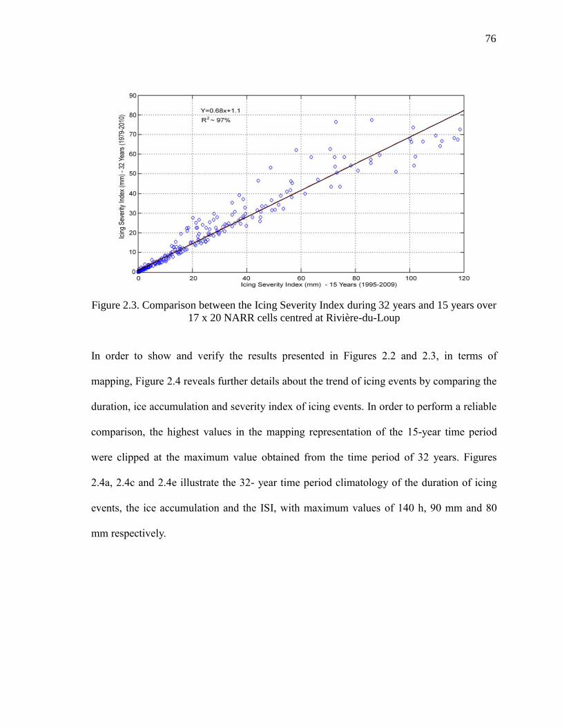
76

Figure 2.3. Comparison between the Icing Severity Index during 32 years and 15 years over

17 x 20 NARR cells centred at Rivière-du-Loup

In order to show and verify the results presented in Figures 2.2 and 2.3, in terms of

mapping, Figure 2.4 reveals further details about the trend of icing events by comparing the

duration, ice accumulation and severity index of icing events. In order to perform a reliable

comparison, the highest values in the mapping representation of the 15-year time period

were clipped at the maximum value obtained from the time period of 32 years. Figures

2.4a, 2.4c and 2.4e illustrate the 32- year time period climatology of the duration of icing

events, the ice accumulation and the ISI, with maximum values of 140 h, 90 mm and 80

mm respectively.

77

Figure 2.4. Comparison between 32 years and 15 years: Duration of icing events (a,b), ice

accumulation (c,d) and Icing severity index (e,f). Colour scales are clipped for the 15 year

period.

78

In addition, the climatology of icing shown in Figures 2.4b, 2.4d and 2.4f

demonstrates more accentuated and intense peaks, with slightly wider features. The

comparison between a 32-year and a 15-year time period, of the same database revealed an

accentuation in the intensity of atmospheric icing (Duration, ice accumulation and ISI)

during the latest 15-year time period. Therefore, in order to assess the severity of icing

events prior to wind farm implantation, it is more appropriate to use 15-year estimation

rather than 32-year estimation, since a 32-year assessment tends to reduce the average of

icing severity.

2.3.3 GEM-LAM and NARR performances

The orography has a significant influence on enhancing the cloud water content,

cloud phase, evaporation and sublimation of cloud hydrometeors. Therefore, it is crucial for

numerical weather modeling to utilize the topography at higher resolution to achieve a

better representation of weather conditions over mountainous and complex terrain areas.

Since this study involves the improvement of the resolution using the output of GEM-LAM

5km rather than those obtained from NARR 32 km data, Figure 2.5 demonstrates the

disparity in topography from different resolutions. This figure is a cross section of the

elevations intersecting the site of Mount-Bélair (~ 480 m) near Quebec City (Canada).

Figure 2.5 shows a noticeable difference between the three topographies. The resolution of

32 km NARR flattens the elevations by averaging out the details within 32 km. With

reference to 1 km, this coarse resolution of 32 km shows underestimations that can reach

400 m, and also potential overestimates that can exceed 200 m. The difference is more

pronounced in the sides of each NARR 32 km cell. Also, when compared to the resolution

79

of 1 km, the resolution of 5 km of GEM-LAM manifests an improvement and considerably

reduces errors in elevations. The real elevation of the Mount-Bélair site is approximately

480 m. The GEM-LAM 1km resolution indicates the best estimate of 453 m followed by

GEM-LAM 5km and NARR 32 km with elevations of 334 m and 147 respectively.

Figure 2.5. Topography Cross Section Viewed by NARR 32km, GEM-LAM 5km and

GEM-LAM 1km

In order to test the sensitivity to the resolution along with meteorological variables

directly involved in calculating icing events, Figure 2.6 shows a comparison of

temperatures at 30 m above ground level obtained from observation at Mount-Bélair,

GEM-LAM 5 km and NARR 32 km. The simultaneous values of a sequence of 22 events

from the three sources occurred during the month of January 1999. Figure 2.6a shows the

temperature values (Y-axis) for each corresponding observation number (X-axis).

Additionally, Figure 2.6b quantifies the differences from the models (NARR, GEM-LAM)

with reference to observations. The behaviour of the curves in Figure 2.6 reveals that the

output of the two models (NARR, GEM-LAM) is warmer than the observations. The

80

results of GEM-LAM 5 km are more accurate compared to those from NARR. The better

consistency of GEM-LAM 5 km with the observations can be explained by the enhanced

resolution of the topography discussed in Figure 2.5 and the more sophisticated

microphysics scheme (M&Y) used with GEM-LAM than that in the NARR

Figure 2.6. Comparison of Temperatures from NARR 32 km, GEM-LAM 5km and

Observation

The results of both Figures 2.5 and 2.6 have shown the improvement brought by

GEM-LAM compared to NARR. It would even be better and more recommended to use

GEM-LAM 1 km; however, the time consuming calculation prevents this option.

Subsequently, this study is limited to the use of GEM-LAM 5 km. One could perhaps

simply replace the GEM-LAM-1km with an air-mass adjustment of the 5 km results to the

1 km terrain (eg. Byrkjedaal, 2013) to reap most of its increased performance. GEM-LAM

has already shown good performance in producing the key parameters that control in-cloud

icing. Through the use of three-level nesting that target the resolution of 1km and

comparison with observation, Yang et al. (2012) investigated in-cloud icing on Mount

Washington and Prescornic (2014) explored icing events on sites in Gapsé. Furthermore,

81

with regard to in-cloud icing in Sweden, Prescornic (2014) compared the performance of

GEM-LAM versus MM5 from a previous study (Drage and Hauge, 2008). Both studies

(Yang et al., 2012; Prescornic, 2014) used similar triple nesting simulation strategies with

resolutions 10 km, 5 km and 1 km and timesteps 300 s, 60 s and 30 s respectively. The

obtained results of 1km resolution demonstrated an agreement with observations over

complex terrains for case studies during time periods less than 24 h. The current study

investigates the climatology of in-cloud icing spanning a long time period. Consequently,

triple nested GEM-LAM simulations that target the resolution of 1 km appear to be very

time consuming. Therefore, the resolution of 5 km that demonstrates an improvement

compared to NARR 32 km is considered in order to cover the climatology during 15 years.

2.3.4 Selection of significant days

After having demonstrated the benefit of use the latest 15 years versus 32 years, and

also the preference of the data of finer scale resolution (GEM-LAM 5km) compared to the

coarse resolution, Table 1 identifies the days selected for downscaling by mesoscale

modeling. Table 1 presents the 114 days that were selected over 15 year period (1995-

2009). With regard to icing severity, these significant days represent an average of 7.6 days

per year. These days were determined based on the ISI over the critical selected sites

(Mount-Bélair, Riviere du Loup, Rimouski, Matane, Gaspé) from the zone of the study.

The selected days are associated with icing events occurrences that have an average daily

icing rate of 0.04 mm h-1

and more. In Table 2.1, it is noticeable that some years have more

than 10 significant severe icing days per month, with January 1998 having the most at 13

significant icing days, followed by 2005, 2006, 2003, 2008 with 12 days, 11 days, 10 days

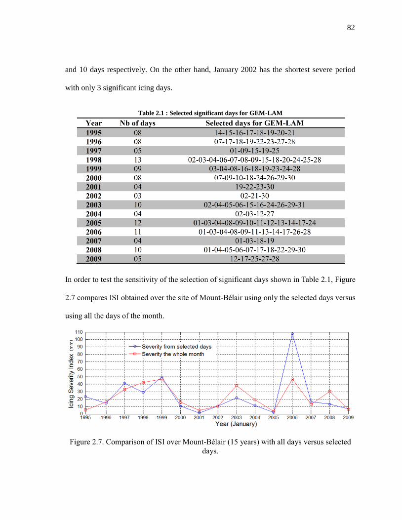
82

and 10 days respectively. On the other hand, January 2002 has the shortest severe period

with only 3 significant icing days.

Table 2.1 : Selected significant days for GEM-LAM

In order to test the sensitivity of the selection of significant days shown in Table 2.1, Figure

2.7 compares ISI obtained over the site of Mount-Bélair using only the selected days versus

using all the days of the month.

Figure 2.7. Comparison of ISI over Mount-Bélair (15 years) with all days versus selected

days.

83

The site of Mount-Bélair is recognized by its frequent and severe icing events. The

tendency of the curves in the comparison in Figure 2.7 shows a satisfying correlation with

slight differences between the ISI values of the same year. Other than 1995, 1997 and 2006,

the ISI of the selected days have an average underestimation of 6.5 mm compared to the ISI

of the entire month. The average ISI over Mount-Bélair is 24.5 mm. Therefore, the

selection of significant days which represents only 24% of the total duration appears to be

adequate in describing the level of Icing Severity.

2.3.5 Mesoscale modeling and simulation setup

To acquire the key meteorological variables for icing events at fine resolution during

the selected days introduced. In the presented Table 2.1, a series of numerical procedures

have been performed. This section describes the steps followed for the mesoscale modeling.

The simulations involve two different grids with three nested domains. As shown in Table

2.2, the simulation is initially (i.e. on the outer domain) driven by NARR data transformed

to polar stereo grids in FST files (Camion, 2012) which is available every 3h with a spatial

resolution of 32 km. Simulations that utilize GEM-LAM are those of the domains D2 and

D3 occupying 124x124 grids 200x200 grids with spacing of 10 km and 5 km respectively.

The timesteps associated with the domains D2 and D3 are 5 min and 1 min respectively.

The objective of the simulations is to obtain output by series of 24 h that correspond

to each of the significant days (Table 2.1). To reduce the numerical errors from the

initialization and to ensure stabilization of the model, the beginning of each simulation is

advanced in time. The first simulation of the domain D2 begins 6 h prior to each target day.

Then the second simulation, which is automatically initialized by the output of the first

84

simulation, starts 3 h prior to each target day (3 h after the first simulation). Both

simulations finish at the end of each target day. Consequently, both simulations for the

domains D2 and D3 cover periods of time of 30 h and 27 h respectively. The target time

period is the last 24 h.

Table 2.2 : Grid setup for the numerical experiment

Table 2.3 : The lowest 17 vertical levels used in GEM-LAM that correspond to ABL

In addition to the advantage of its high customizable resolution, The GEM model

provides output along the atmospheric column at 56 terrain-following vertical levels above

the ground. With regard to the atmospheric boundary layer (ABL), Table 2.3 shows the

85

lowest 17 vertical levels, their corresponding hybrid levels and above ground levels (AGL).

The present study uses the versions 4.2 of GEM of Environment Canada with the

physics package RPNPHY_5.2.1. The two simulation zones share the same center, which is

located near the city of Rivière-du-Loup (QC- Canada) defined by the latitude 47.83° and

the longitude -69.53°. For the purpose of numerical optimization and to prevent the

narrowing effect within the calculation domains toward the North, the longitude of the

same center is rotated 20.47° in order to ensure that the numerical equator is oriented

toward the East while passing through the Rivière-du-Loup location.

Given the required variables for the calculation of icing events and the location of the

target domains, the configuration is based on the double moment (DM) condensation

scheme of Milbrandt and Yau (Milbrandt and Yau, 2005) and the activation of CCN.

Commonly, continental air masses carry much more aerosols that serve as cloud

condensation nuclei (CCN) compared to maritime air masses. Therefore, with the same

moisture, Maritime air masses (CCN ~ 10 to 100 cm-3

) originate larger droplets compared

to Continental air masses (CCN ~100 to 1000 cm-3

) (Pruppacher and Klett, 2010). More

precisely, for the simulation of this study, Maritime air masses considered by GEM-LAM

use a CCN concentration of 80 cm-3

.

Both domains D2 and D3 of nested simulations are presented in Figure 2.8 by the two outer

squares, which are geometrically correlated. D2 and D3 occupy areas of 1240x1240 km2

and 1000x1000 km2 respectively. D1, the NARR domain, covers more than the entire area

depicted in Figure 2.8. Furthermore, within D3 Figure 2.8 illustrates an additional

delineation represented by a slanted rectangular shape. This third area that covers the Gaspé

86

Peninsula and its surroundings is the target zone to be used for the purpose of comparison

with the results shown in Figure 2.4 and also the results of a previous study (Lamraoui et

al., 2013). The target zone occupies an area of approximately 640x544 km2 (i.e. the 20x17

NARR cells mentioned in section 2).

Figure 2.8. Simulation domains and target zone

The simulations of GEM-LAM were realized using the cluster Boreas (ETS –

University of Quebec) which is a high performance supercomputer cluster with 464

processors (58 nodes) in parallel with 928 GB of RAM, infiniband technology and

equipped with Sun Grid Engine (SGE) batch-queuing system.

For this study, eight simulations were launched simultaneously and continuously, until

covering all target days. Each simulation made use of one node (8 processors) and lasts

87

approximately for 8 h including both domains D2 and D3 with 360 timesteps, 1620

timesteps respectively.

2.3.6 Statistics and cloud microphysics properties

After completing the simulations and retrieving the required variables for the

calculation of icing events, Figure 2.9 was prepared to scrutinize the microphysical

properties of supercooled clouds associated with the occurrence of icing events. Moreover,

Figure 2.9 depicts statistically the interrelationship between the key parameters that

determine the intensity of icing events. In this figure, the variables SLW, median volume

diameter (MVD), air temperature and wind speed are derived from the simulation of the

domain D3, and more precisely at the levels 21 m, 36 m, 57 m, 87 m and 128 m (Table 2.3).

All the obtained data of this section correspond to the 114 significant icing days, with a

frequency of one value each 10 min for each grid point of the total 200x200 grid points

(domain D3). Since this study focuses on the range of temperatures below zero, only the

data occurring within this range are considered.

88

Figure 2.9. Statistics of meteorological icing parameters

The histogram and the cumulative sum of SLW indicate that smaller values of SLW

that are less than 0.05 g m-3

are more frequent with a percentage that exceeds 50%.

Moreover, SLW between 0.1g m-3

and 0.3g m-3

manifest a frequency of 30%. Statistically,

SLW that are equal or greater than 0.4 g m-3

have insignificant frequency.

With respect to the obtained spectrum of MVD, the values around 15 μm take the

lead in terms of frequency. In addition, within a relatively broader spectrum of MVD, the

range of MVD between 10 μm and 20 μm appears with a frequency that exceeds 30% of

the occurrences. Consequently, this finding demonstrates that the typical MVD that is

associated with near surface supercooled clouds and icing events is approximately 15±5μm.

89

Small droplets with MVD less than 10 μm show a frequency around 18%. The frequency of

MVD ranging from 30 μm to 50 μm is around 23%. Supercooled droplets with MVD larger

than 50 μm are considered by the World Meteorological Organization as SLD. Due to their

hazardous impact on structures; SLD has been studied with a particular intention. From this

study, the frequency of SLD in Figure 2.9 indicates a percentage that exceeds 5%. Also, the

whole spectrum of MVD is capped approximately by MVD = 70 μm.

In addition to the variables from cloud microphysics (SLW, MVD), the

meteorological dynamic parameters (temperature and wind speed) are significantly

influential in quantifying icing events. By taking into account the atmospheric layer

considered in this section, the histogram of temperature reveals that the supercooled liquid

cloud droplets occur exclusively between -15 °C and 0 °C. More specifically, the

temperatures between -5 °C and 0 °C encompass 75% of all occurrences, followed by the

ranges [-10 °C to -5 °C] and [-15 °C to -10 °C] with approximate frequencies around 20%

and 5% respectively. The histogram of the wind speed in Figure 2.9 indicates that over 50%

have wind speeds below 5 m s-1

. Wind speeds ranging from 5 m s-1

to 10 m s-1

have a

frequency of 30%. On the other hand 10% of the frequencies are assigned to the range

between 10 m s-1

and 15 m s-1

. Furthermore, the corresponding weibull distribution to the

wind speed histogram indicates a shape coefficient of 5.64 and a scale coefficient of 1.6.

All values of wind speeds are capped at around 15 m s-1

.

2.3.7 Vertical profile of icing events climatology

In order to investigate the spatial distribution of the climatology of icing events and

its vertical evolution along the atmospheric column, Figure 2.10 examines independently

90

the duration of icing events, ice accumulation, the frequency of occurrences of different

severity classes of icing severity (Trace, Light, Moderate, Severe and Extreme), and

corresponding topography.

91

Figure 2.10. Vertical profiles of high resolution 15-year climatology of icing events: (a)

severity classes (b) duration of icing events (c) ice accumulation (d) Topography from

GEM-LAM5km

92

The results in this figure are derived from all points in the simulation of domain D3

for the significant days and from NARR (1000 mb) for the insignificant days. The results

cover the time period of 15 years (1995-2009) and represent only GEM-LAM model levels

(10 m, 57 m, 87 m, 128 m and 179 m). For the purpose of comparison, the duration of icing

events and ice accumulation in Figure 2.10 are capped by 140 h and 50 mm respectively.

The curves located in the left side of Figure 2.10 represent the percentage of the frequency

of each icing severity class. From the interpolation of model levels, the occurrence

frequency of each severity class is derived along the atmospheric layer from 10 m until 200

m with an interval of 10 m. The vertical distribution of icing results in Figure 2.10 reveals a

disparity between the climatology profiles of the ice accumulation and the duration of icing

events. The pattern of the duration of icing events indicates a steady behaviour without

showing a significant variation along the studied atmospheric layer. On the other hand,

toward higher elevations, the subfigures of the ice accumulation of each layer demonstrate

a gradual intensification.

Lamraoui et al. (2013) have subdivided the intensity of icing events in 5 classes

based on the accumulation rate. Therefore, regarding the frequency, Figure 2.10 (left side)

introduces the vertical profiles of each of these classes. Within the lowest layer above

ground between 10 m and 60 m, each of severity classes has a vertical profile of

frequencies that are approximately steady, with values around 75% of Trace, 10% of Light

and Moderate, between 2% and 3% of Severe and around 1% of extreme. Figure 2.10

indicates that Trace (weakest icing class) is the dominating class all along the atmospheric

93

layer between 10 m and 200 m. Starting at level of 60 m above ground, the class Trace

decreases upward to reach 35% of the occurrences. Light and Moderate classes manifest an

increase of frequency starting from level 60 m. On the other hand, the classes Severe and

Extreme demonstrate increasing occurrences above 100 m. In this range of elevations and

with different tendency of classes, Light and Moderate severities show increasing

frequencies that reaches 23% and 27 % respectively, at the elevation of 200 m. Meanwhile,

the severe and extreme classes start to manifest a different behaviour, only above the height

of 100 m. Compared to previous classes, these intense classes increase slowly at higher

elevations to reach 13 % and 4 % respectively, at the height of 200 m.

2.3.8 Icing severity index at fine scale resolution

This section discusses the advantages of using the mesoscale Model (GEM-LAM)

with its advanced microphysics scheme on quantifying icing events, compared to the use of

NARR. Therefore, to compare the results of these two data sources, Figure 2.11, illustrates

the climatology of the ISI derived from (a) NARR data at 1000 mb and (b) GEM-LAM-

5km at 1000 mb.

94

Figure 2.11. 15-year climatology of icing Severity Index at 1000 mb: (a) NARR 32 km, (b)

GEM-LAM 5km

The two sub-figures in Figure 2.11 represent the same pressure level of 1000 mb. It

is noticeable that Figure 2.11b reveals more details at smaller scale. Small areas of fine

scale resolution that are shown in Figure 2.11b are mainly Continental and manifest a

proportional response to the topography.

The small intense areas are located mainly in mountainous regions, such as in the

Gaspé Peninsula. It is noticeable that Murdochville and its surroundings have an intense

icing climate. Also an intense ISI extends along the mountain ridge from the National Park

of Gaspésie until the Matane Wildlife Reserve.

On the west side of the St Lawrence River and more precisely in the North of the

Saguenay region, a significant icing climate is marked over the National Park of Monts-

Valin including the Monts-Valin themselves. Southward and between the region of

Saguenay and Quebec City, the Laurentian Wildlife Reserve shows significant values of

ISI.

95

Regions with very intense icing severity that occupy larger areas shown in Figure 2.11b are

found mainly in the National Capital region, including the site of Mount-Bélair, followed

by the region of Chaudière-Appalaches and the Lower St. Lawrence Region especially

between Rimouski and Matane including Mont-Joli and continuing Southward to reach the

north of the province of NewBrunswick.

Moreover, both Figure 2.11a and b demonstrates that regions of the North-east and the

centre of the province of New Brunswick manifest very high icing severities. However,

2.11b exclusively manifests a high icing severity which covers the Mount Carleton

Provincial Park and its surroundings including the Mount-Carleton with its summit that

exceeds 2600 ft, a zone that encompasses the Caribou Wind Park.

Besides Canadian regions, Figure 2.11b reveals a narrow zone with very localized and

intense ISI in the state of Maine (USA) on the Mount Katahdin, the highest mountain in

Maine with an elevation over 1600 m.

In order to target the wind industry, Figure 2.12 focuses on three critical levels

above ground of ice accretion on a typical wind turbine with a hub of 80 m and tips of the

blades in sweeping motion within the atmospheric layer between 40 m and 120 m.

Therefore, this figure represents the climatologies of ice accumulation and duration of icing

events at these levels. The accumulation and the duration of icing demonstrate that the level

of 120 m contains the highest values.

96

Figure 2.12. 15-year climatology of ice accumulation and duration of icing events at 40m,

80m and 120

The mapping in Figure 2.12 demonstrates higher response of ice accumulation to

topography compared to duration of icing events which shows larger areas. With regard to

97

the duration of icing events, the peak values show persistance in all levels. Meanwhile, very

localized zones with more elevated topography show an increase in ice accumulation at

higher altitudes.

Figure 2.13 illustrates the vertical profile of the mean values of ice accumulation

and duration of icing events at each level starting from 10 m to 200 m. This statistical

estimation covers the entire D3 area and occupies an area of 1000x1000 km2. Also, in

Figure 2.13, the ice accumulation shows a gradual intensification toward higher elevations.

On the other hand, the duration of event shows that increase only starting from the level of

60 m. The range of the mean values of ice accumulation vary from 6 mm at the level of 10

m to reach 17.2 mm at 200 m. On the other hand, the mean values of the duration of icing

events is approximately 39 h below 60 m. Beyond the level of 60 m the duration increases

to reach 61 h at 200 m.

98

Figure 2.13. Vertical profiles of ice accumulation and duration of icing events between 10

and 200 m.

Following the presentation of results of the accumulation of ice and the duration of

icing events, Figure 2.14 shows the climatology of the ISI during the 15-year time period

from 1995 to 2010. The ISI combines the accumulation and duration by joining them with

weighting factors that reflect the influence of the accumulation rate, the liquid water

content and the duration of icing event, to assess the level of the severity of icing events.

Given the typical operational height 80 m (Hub) of wind turbine, Figure 2.14 illustrates the

ISI at that height.

99

Figure 2.14. 15-year climatology of icing Severity Index at 80 m.

This map shows two categories of regions with extreme ISI; large areas and very

localized areas. In reference to large areas, Figure 2.14 shows the region that extends from

the Moncton area in New Brunswick to Amherst in Nova Scotia, the northern region of the

state of New York between St Lawrence River and the west of Adirondacks, The

Montérégie area in Quebec, Chaudière-Appalaches, The north of lac St-Jean (Saguenay)

and the large region that is located in the east of the James Bay. On the other hand,

numerous small extreme areas are unevenly spread on the map and are mainly found in the

Gaspé peninsula and northeast of the province of Quebec. Murdochville which is a typical

complex field site indicates a very pronounced ISI. The Caribou wind park in the province

of New Brunswick is definitly exposed frequently to severe icing events. Also, it is

100

noticeable that the mountainous regions of New York, Vermont, New Hampshire have high

values of ISI, except for elevated areas between the Mt Washington and the Mt Kathadin

(Maine).

2.4 Conclusion

The leading idea of this study is based on the identification of in-cloud icing events

derived from non-precipitating supercooled cloud droplets by locating their occurrences,

quantifying their intensities and then determining their durations. In order to achieve this

goal, the present study utilized an original hybrid approach that provided fine resolution

climate representations of icing events. In a previous study by the same authors the use of a

32-year time period (1979-2010) was applied to map the atmospheric icing severity. The

current study was focused on the last 15 years of this time period, specifically from 1995 to

2009.

A statistical assessment showed that the month of January had an average of 7.6

icing days over the Gaspé Peninsula and its surroundings, including Eastern New

Brunswick. The use of NARR data indicated a limitation in capturing icing events over

complex terrains. Therefore, the involvement of finer scale modeling is crucial for adequate

representation of atmospheric phenomena, particularly near the surface. The simulations are

driven by NARR data and implicate the use of a limited-area version of GEM model with

multi-nested domains that have spatial resolutions of 10 km and 5 km and temporal

resolutions of 300 s and 60 s respectively.

The simulations of GEM-LAM for the entire 15-year time period are very time

101

consuming, therefore this study implicated a hybrid approach that involved only the

significant icing days in the GEM-LAM calculations. In turn, icing calculations for the

non-significant icing days in this time period used data directly from NARR. Consequently,

the final product represents the entire 15 years period (1995-2009) with finer scale

resolution details of icing events. In addition, since NARR data is not directly compatible

for the use of GEM model, conversion tools (projection, format) were created to meet the

operational requirements of GEM-LAM.

The findings of this study during the significant icing days revealed typical

supercooled droplet sizes associated with near-surface icing events with 30% of MVD

around 15 μm±5 μm and 5% of supercooled large droplets (MVD>50μm). Furthermore, the

temperature range is mainly dominated by values between -5 ° C and 0 ° C, which represent

75% of occurrences. Ultimately, with the use of an original strategy, this study explored the

icing events at fine scale resolution and in three dimensions. The results indicated the

importance of the altitudes 60 m and 100 m that mark substantial transitions in the vertical

profile of the severity classes. Moreover, toward higher elevations, the duration of icing

events and the ice accumulation indicated higher values at higher elevations. Conclusively,

the data at fine scale resolution contributes significantly in revealing more details of

orographic clouds and condensation that lead to larger cloud droplet sizes and consequently

more ice accumulation.

102

2.5 References

Ahrens, C.D., 2007. Meteorology Today: An Introduction to Weather, Climate, and the

Environment, 8th ed. Thomson Brooks/Cole, Belmont, CA 537.

Bennartz, R., Shupe, M. D., Turner, D. D., Walden, V. P., Steffen, K., Cox, C. J., Kulie, M.

S., Miller, N. B. and Pettersen, C., 2013. July 2012 Greenland melt extent enhanced by

low-level liquid clouds. Nature. 496, 83-6.

Bernstein, B.C., Tiffany, A., Omeron, A., Politovich, M.K. and McDonough, F., 1998.

Surface weather features associated with freezing precipitation and severe in-flight aircraft

icing. J. Atmos. Res. 46, 57–73.

Bernstein, B.C., Ratvasky, T.P., Miller, D.R. and McDonough, F., 2000. Freezing Rain as

an In-Flight Icing Hazard. (NASA TM-2000-210058, June 2000).

Bernstein, B.C., Wolff, C.A. and McDonough, F., 2007. An inferred climatology of Icing

conditions aloft, including supercooled large drops. Part I: Canada and the Continental

United States. J. Appl. Meteor. Climatol. 46, 1857–1878.

Boudala, F. S., Isaac, G. A., Cober, S. G. and Fu, Q., 2004. Liquid fraction in stratiform

mixed-phase clouds from in situ observations. Q. J. R. Meteorol. Soc. 130, 2919-2931.

Byrkjedal., Ø., 2013. Icing map of Sweden, (Winterwind, Östersund, 12.02.2013)

Camion, A., 2012. La modélisation des événements de givre atmosphérique: Interpolation

de la NARR pour l’utilisation de GEM. (MSc thesis). University of Quebec, École de

Technologie Supérieure, 255.

Carrière, J.M., Lainard, C., Le Bot, C. and Robart, F., 2000. A climatological study of

surface freezing precipitation in Europe. Meteorol. Appl. 7, 229–238.

Cober, S.G., Isaac, G.A., Strapp, J.W., 2001. Characterizations of Aircraft Icing

Environments that Include Supercooled Large Drops. J. Appl. Meteor. 40, 1984–2002.

Cortinas, J.V; Bernstein, B.C; Robbins, C.C. and Strapp, J.W. 2004. An analysis of

freezing rain, freezing drizzle, and ice pellets across the United States and Canada: 1976-

90. Weather and Forecast. 19 (2) 377-390

Debenedetti, P.G., 1996. Metastable Liquids: Concepts and Principles. Princeton University

Press, Princeton, NJ (400 pp.).

Dee, D.P., Uppala, S.M., Simmons, A.J., Berrisford, P., Poli, P., Kobayashi, S. and Andrae,

U., Balmaseda, M.A., Balsamo, G., Bauer, P., et al., 2011. The ERA-Interim reanalysis:

103

configuration and performance of the data assimilation system. Q. J. R. Meteorol. Soc. 137,

553–597.

Drage, M.A. and Hauge, G., 2008. Atmospheric icing in a coastal mountainous terrain.

Measurements and numerical simulations, a case study. Cold Reg. Sci. Technol. 53(2),

150-161.

Fernández-González S., Valero F., Sánchez J.L., Gascón E., López L., García-Ortega E.

and Merino A., 2014. Observation of a Freezing Drizzle Episode: A Case Study. Atmos.

Res. 149, 244-254.

Fikke, S.M., 2005. Modern meteorology and atmospheric icing. In: Proc 11th IWAIS,

Montreal, Canada. June 2005. Paper IW73.

Heymsfield, A. J., Miloshevich, L. M., Slingo, A., Sassen, K. and Starr, D. O. C., 1991. An

Observational and Theoretical-Study of Highly Supercooled Altocumulus. J. Atmos. Sci.

48, 923-945.

Illingworth, A.J., Hogan, R.J., O’Connor, E.J., Bouniol, D., Brooks, M.E., Delanoë, J.,

Donovan, D.P., Eastment, J.D., Gaussiat, N., Goddard, J.W.F., et al., 2007. Cloudnet—

Continuous evaluation of cloud profiles in seven operational models using ground-based

observations. Bull. Am. Meteorol. Soc. 88, 883–898.

Jacobson, M.Z., 2005. Fundamentals of Atmospheric Modeling. Cambridge University

Press, Cambridge (813 pp.).

Korolev, A. V. and Isaac, G. A., 2000. Drop growth due to high supersaturation caused by

isobaric mixing. J. Atmos. Sci. 57, 1675–1685.

Laakso, T., Baring-Gould, I., Durstewitz, M., Horbaty, R., Lacroix, A., Peltola, E.,

Ronsten, G. and Tallhaug, L., T., Wallenius, 2010. State-of the- art of wind energy in cold

climates, In : Work. Pap. 152, VTT Tech. Res. Cent. of Finl., Esbo, Finland.

Laflamme, J., 1993. Spatial variation of extreme values in the case of freezing rain icing.

In : Proc 6th IWAIS, Budapest, Hongrie, 19–23.

Lamraoui, F., Fortin, G., Benoit, R., Perron, J., and Masson, C, 2013. Atmospheric icing

severity: Quantification and mapping. Atmos. Res. 128, 57–75.

Lamraoui, F., Fortin, G., Benoit, R., Perron, J., and Masson, C., 2014. Atmospheric icing

impact on wind turbine production. Cold Reg. Sci. Technol. 100, 36–49.

Lasher-Trapp, S., Anderson-Bereznicki, S., Shackelford, A., Twohy, C.H. and Hudson, J.

G., 2008. An Investigation of the Influence of Droplet Number Concentration and Giant

104

Aerosol Particles upon Supercooled Large Drop Formation in Wintertime Stratiform

Clouds. J. Appl. Meteor. Climatol. 47, 2659-2678.

Lau, K. M. and Wu, H. T., Warm rain processes over tropical oceans and climate

implications. Geophys. res. lett., 30, 2003, http://dx.doi.org/10.1029/2003GL018567.

Marwitz, J. D., Politovich, M., Bernstein, B., Ralph, F., Neiman, P., Ashenden, R. and

Bresch, J., 1997. Meteorological conditions associated with the ATR72 aircraft accident

near Roselawn, Indiana, on 31 October 1994. Bull. Am. Meteorol. Soc. 78, 41–52.

Milbrandt, J. and Yau, M. K., 2005, A multi-moment bulk microphysics parameterization,

part I: Analysis of the role of the spectral shape parameter, J. Atmos. Sci. 62, 3051–3064.

Morrison, H., de Boer, G., Feingold, G., Harrington, J., Shupe, M.D. and Sulia, K., 2011.

Resilience of persistent Arctic mixed-phase clouds. Nat. Geosci. 5, 11-17.

Murakami, M., Yamada, Y., Matsuo, T. Mizuno, H. and Morikawa, K., 1992.

Microphysical structures of warm-frontal clouds. The 20 June 1987 case study. J. Meteor.

Soc. Japan. 70, 877–895.

Pobanz, B.M., Marwitz, J.D. and Politovich, M., 1994. Conditions associated with large-

drop regions. J. Appl. Meteor. Climatol. 33, 1366-1372

Politovich, M K., 1989 Aircraft Icing Caused by Large Supercooled Droplets, J. Appl.

Meteor. Climatol. 28, 856-868.

Politovich, M.K.,1996. Response of a research aircraft to icing and evaluation of severity

indices. J. Aircraft. 33, 291–297.

Prescornic, D., 2014. Modélisation méso-échelle d’événements de précipitation givrante

pour un parc éolien. MSc Thesis . University of Quebec, École de Technologie Supérieure.

pp 255

Pruppacher, H.R. and Klett, J.D. 2010. Microphysics of Clouds and Precipitation.

Atmospheric and Oceanographic Sciences Library, Vol. 18. 2nd ed. (976 pp.).

Rasmussen, R. M., Bernstein, B. C., Murakami, M., Stossmeister, G., Reisner, J. and

Stankov, B., 1995. The 1990 Valentine’s Day Arctic outbreak. Part I: Mesoscale and

microscale structure and evolution of a Colorado Front Range shallow upslope cloud. J.

Appl. Meteor. 34, 1481–1511.

Rock, P.A., 2003. Chemical Thermodynamics, University Science Books, USA (548 pp.).

Sand, W. R., Cooper, W. A., Politovich, M. K. and Veal, D. L., 1984. Icing conditions

encountered by a research aircraft. J. Climate Appl. Meteor. 23, 1427–1440.

105

Schemenauer, R.S. and Cereceda, P., 1994. A Proposed Standard Fog Collector for Use in

High-Elevation Regions. J. Appl. Meteor. Climatol. 33 (11), 1313-1322.

Shin, J., Berkowitz, B., Chen, H. and Cebeci, T., 1991. Prediction of ice shapes and their

effect on airfoil performance. AIAA 29th Aerospace Sciences Meeting, Reno, NV, Paper

AIAA-91-0264, 21 pp.

Shupe, M. D., 2011. Clouds at Arctic atmospheric observatories. Part II: Thermodynamic

phase characteristics. J. Appl. Meteor. Climatol. 50, 645–661.

Stuart, R.A. and Isaac, G.A., 1999. Freezing precipitation in Canada. Atmosphere-Ocean

37–1, 87–102.

Turner, D.D., 2005. Arctic Mixed-Phase Cloud Properties from AERI Lidar Observations:

Algorithm and Results from SHEBA. J. Appl. Meteor. Climatol. 44(4), 427-444.

Yang, J., Jones, K. F., Yu, W. and Morris, R., 2012. Simulation of in-cloud icing events on

Mount Washington with the GEM-LAM, J. Geophys. Res., 117, D17204.

CHAPTER 3

ATMOSPHERIC ICING IMPACT ON WIND TURBINE PRODUCTION

This Chapter is published in the form of an original scientific article

in the journal of

Cold Regions Science and Technology, 2014, vol 100, p. 36-49

dx.doi.org/10.1016/j.coldregions.2013.12.008

Fayçal Lamraoui 1*

, Guy Fortin 2, Jean Perron 1, Robert Benoit

3, Christian Masson

3

1 The Anti-Icing Materials International Laboratory, University of Quebec at Chicoutimi

2 Bombardier Aerospace

3. École de technologie supérieure, University of Quebec

*Corresponding Author address:

Fayçal Lamraoui

The Anti-Icing Materials Internationa Laboratory, University of Quebec at Chicoutimi 555, boulevard de l'Université, Chicoutimi, QC, G7H 2B1 Canada

Email: faycal.lamraoui@gmail.com

107

3. ATMOSPHERIC ICING IMPACT ON WIND TURBINE

PRODUCTION

Abstract

Wind turbine performance depends mainly on the wind speed and aerodynamics of

blades. The roughness generated from ice accretion can significantly reduce the

aerodynamics and consequently the power production of the wind turbine. This study

locates the glaze and rime ice on the blade, to detect the critical zones involved in

significant power production loss. On the blade, the distribution of the elementary power

production as well as the type and thickness of the accreted ice are inconsistent. Under

icing conditions, the outer section of the blade starting fromthe radial position r/R=0.8

contribute significantly to the blades aerodynamics. The freezing fraction is unevenly

distributed; since it initially forms rime ice near the root and then glaze toward the tip of the

blade. The critical freezing fraction 0.88 associated with the double horn ice shape is

spatially limited and occupies a restricted segment on the blade and gradually moves

towards the tip with decreasing temperature. With the use of power degradation analogy

with sub-scaled rotor blades of a helicopter under icing conditions, a power loss factor is

introduced to quantify and locate power loss along the blades of wind turbines. The study is

based on four values of liquid water content that delineate five classes of icing severity.

Including power loss factor, the most significant power loss that corresponds to freezing

fraction 0.88 is found to be located at r/R ~ [0.93 0.96] which corresponds to T = -2.6 °C, -

4.5 °C, -12 °C, and -20 °C and for liquidwater content LWC=0.04 g·m-3

, 0.07 g·m-3

, 0.2

g·m-3

, and 0.36 g·m−3 respectively. The resulted power degradation can reach a maximum

of 40%. Locally it is the shape rather than the thickness of ice that causes more power loss;

meanwhile when considering the whole blade, power degradation is controlled mainly by

ice thickness regardless of the type of ice. The results obtained can help the setup of a

sensor that triggers the ice-protection system upon detection of critical freezing fraction.

.Keywords: Ice accretion, Wind turbine, Re-analysis, Atmospheric icing climatology

108

3.1 Introduction

Numerous cold climate countries already utilize and will progressively make more

use of wind energy, because of their propitious high wind potential. Cold climate regions

represent an unavoidable beneficial environment for wind energy. For this reason and in

order to maintain maximum extraction of power production, wind turbine manufacturers

including blade's airfoil designers are required to accommodate the hazardous conditions of

atmospheric icing events. Cold regions with higher altitudes represent the best sites for

wind farms; wind speed increases approximately by 0.1 m·s-1

each 100 m of altitude within

the first 1000 m (Parent and Ilinca, 2011). Colder regions are characterized by a potential of

wind power 10% higher than other regions, because of their higher air density. Since cold

air is denser than warm air, it increases the kinetic energy of windwhich leads to further

power production of wind turbine (Fortin et al., 2005). Commonly wind turbine farms are

located in coastal or mountainous areas; these regions are exposed frequently to icing

events during the cold seasons (Tammelin and Säntti, 1998). Besides freezing precipitation,

low-level stratus clouds at subzero temperatures and more specifically fog cause serious

challenges to land, air and sea transportation, and greatly affect the wind turbine industry

(Bendix et al., 2005). Ice accretion on the blade of awind turbine reshapes the blade airfoil

and affects negatively its aerodynamic properties. The damaging effect of atmospheric

icing on wind turbine production is not limited to severe icing events and high amount of

ice accretion; even small amounts of ice on the leading edge of the blade degrades

drastically its aerodynamic characteristics and consequently the expected electric power

(Jasinski et al., 1998; Marjaniemi and Peltola, 1998). Furthermore, icing events affect wind

109

assessment and the performance of wind farms by generating measurement errors, power

losses, premature mechanical failures, electrical failure and safety hazards (Parent and

Ilinca, 2011; Seifert et al., 2003). Besides load asymmetry, vibration and safety hazards,

certain icing conditions may cause significant economic losses for the wind turbines

industry.

The occurrences of severe icing events necessitate setting the wind turbine on non-

operational mode in order to minimize ice accretion and its aerodynamic effects. In general,

without the de-icing or the anti-icing procedures, ice accretion on the blades remains for a

significantly longer period than duration the icing event itself (Laakso et al., 2010). Bose

and Rong (1990) demonstrated that even a vestige of roughness generated from the smallest

ice accretion on a wind turbine blade will weaken the expected wind energy by up to 20%.

More precisely, wind energy that is weakened by ice accumulation and duration of icing

events encounter power losses that range between 0.005% and 50% of the annual

production (Botta et al., 1998; Laakso and Peltola, 2005; Tammelin and Säntti, 1996). An

experimental study achieved by Antikainen and Peuranen (2000) on wind turbine blades

showed that icing events that last at least a fewhours, generate a mass and aerodynamic

unbalance. Furthermore, in case this asymmetrical state persists for a long period (days or

weeks), the power production and turbine lifetime drop considerably. A costly anti-icing

strategy is used to minimize icing effects; however it is not a practical solution for icing

concerns since this strategy can consume approximately 25% of the energy produced by the

wind turbine (Makkonen and Autti, 1991). Previous studies have looked at wind turbine

aerodynamics and performance degradations. The investigations and analysis involved the

110

different effects of rime and glaze (Hochart et al., 2008), by analyzing ice accretion effects

on lift to drag ratio (Hochart et al., 2008; Jasinski et al., 1998) and power degradation

(Dierer et al., 2009; Jasinski et al., 1998). Hochart et al. (2008) analyzed in-fog icing

measurements from the Murdochville wind farm in the Gaspé Peninsula (Canada). The

study revealed a significant torque reduction located on the outer third of the blades. In

order to counterbalance the icing effect on the blade, the active heating system on the blade

represents an effective solution (Parent and Ilinca, 2011) that needs further devoted

research to lower its cost. Under icing conditions, Dierer et al. (2009) indicated that the

anti-icing heating system reduces the loss of the annual power production 3.5 %, compared

to 10 % of annual loss without a heating system. Also, under rime conditions, Jasinski et al.

(1998) demonstrated that the performance loss of wind turbine can reach 20 %. In

attempting to assess the long term severity of atmospheric icing for wind turbines,

Lamraoui et al. (2013) presented the climatology of icing severity for wind turbines,

using 32 years (1979–2010) of meteorological data extracted from the North American

Regional Reanalysis (NARR). In general, the severity assessment of icing event depends on

the field of application and the targeted problem being considered. The icing severity index

introduced by Lamraoui et al. (2013) represents the varying degrees of icing severity that

combine different threat factors by weighting each according to a scale of seriousness.

In collaboration with Bell Helicopter, Fortin and Perron (2009) performed an

experimental study based on a spinning rotor blade developed at the Anti-icing Materials

International Laboratory.

111

The objective of that study is to investigate ice physics, low energy de-icing system

and ice-phobic coatings for small helicopters. Compared to a clean blade, the power

required to rotate an iced blade increases with decreasing air temperature until reaching its

maximum at about 5200 W that corresponds to a critical freezing fraction of 0.88. This

critical value is associated with the formation of a double horn ice shape. Beyond the

maximum of 5200 W, the required power decreases with decreasing air temperature to

reach its minimum at about 1200 W. This minimum power occurs when the blades are

clean without ice accretion. The effect of air temperature on power is due to the ice shape

change with the freezing fraction which in turn depends on air temperature and liquid water

content. The partial freezing of water initiates a water runback that freezes afterward,

causing an airfoil reshape and aerodynamic degradation. With the use of the results of

Fortin and Perron (2009), the present study focuses on identifying crucial parameters that

control the type of ice accretion on the blades of a wind turbine which causes high power

loss such as: Freezing fraction, liquid water content, temperature, and the critical radial

position on the blade. Typical values of icing events were extracted and calculated from

NARR data during a time period of 32 years. The current paper also investigates and

attempts to estimate the contribution of each localized zone along the blade of the wind

turbine to power losses that occur under different icing conditions.

112

3.2 Methodology

The models used for the current study attempt to involve more relevant parameters,

in order to improve the assessment of the severity of icing events, and more specifically the

production loss of wind turbines caused by ice accretion. In addition to the liquid water

content and the duration of icing events for different icing severity classes involved in the

quantification and the assessment of the icing severity index (Lamraoui et al., 2013), the

present study focuses on exploring the aerodynamic degradation distribution along the

blade, under different meteorological conditions and geometries of the blades. In order to

cover a typical range of liquid water contents and various severity classes (Fikke et al.,

2006; Lamraoui et al., 2013), the values of LWC 0.04 g·m-3

(light), 0.07 g·m-3

(moderate),

0.2 g·m-3

(severe), 0.36 g·m-3

(extreme) were considered for ice calculation. Under icing

conditions, the distribution of the electric energy production along an optimal blade design

was calculated, in order to locate the critical position on the blade that causes the highest

power loss during icing events. The use of ice accretion and power loss models with

different values of meteorological and geometric parameters enables the exploration to help

locate the aerodynamic and mechanical effects along the blade. Several studies (Hochart et

al., 2008; Lamraoui et al., 2013) have associated the value of liquid water content 0.2 g·m-3

to representative occurrences of atmospheric icing over Murdochville, and to the average of

maximum values during winter months over Mount Bélair (Canada). Therefore, a particular

intention was given to production losses that are associated this typically assumed liquid

water content. Unlike helicopters that require power to rotate, wind turbines rotate to

provide power. Due to the lack of studies that investigate the impact of freezing fraction on

113

wind turbines production, the effect of freezing fraction on power requirements for

helicopter is projected on wind turbine power production. To begin, this study identifies the

critical location which corresponds to the most aerodynamically hazardous freezing fraction

(Fortin and Perron, 2009) on the blade that holds the maximumpower loss. Then, the

corresponding temperatures for typical liquid water contents are determined, and finally

power loss is evaluated (Fortin and Perron, 2009).

3.2.1 Generic wind turbine

The investigation was carried out on a generic horizontal axis wind turbine which is

based on V80-1.8 MW Vestas characteristics. This type of wind turbine is commonly used

in the province of Quebec (Canada). This wind turbine is characterized by a diameter of 80

m and a rated power of 1.8 MW that corresponds to a rated wind speed of 14 m·s-1

. The

minimum wind speed at which the wind turbine starts to be operational is 4 m·s-1

. The

blades have a variable pitch angle that corresponds to prevailing winds. The wind turbine

rotates at approximately 16 rpm (Vestas).

3.2.2 Blade

The generic blades have a radius of 40 m and are designed to provide more power

and to minimize mechanical strains and sound. Since the blade design with more efficiency

is complex and costly, a simplified alternative that represents a linear variation of the chord

along the span was suggested (Burton et al., 2001).

3.2.3 Chord

As shown in Figure 3.1, at 5m away from the hub and along the span, the chord

starts with the longest value of 3.5 m and it decreases linearly along the span until reaching

114

its minimum value of 0.5 m at the tip of the blade. The length of the chord along the span

was determined based on Eq. (1). x[m] is the position along the span that varies from 5 m to

40 m.

𝑐 3 5 (

5) (5 − 𝑥) (1)

The first 5 m from the hub of the blade are not considered because of the cylindrical shape

and its insignificant contribution to power production.

Figure 3.1. Chord variation along the span

3.2.4 Airfoil

In order to substitute NACA 44xx airfoil, Danish wind turbine designers started to

use NACA 63(2)-xx airfoils that showed a reduced sensitivity to leading edge roughness.

115

According to Abbot and von Doenhoff (1959) and Hansen (2008), wind turbine blades are

often designed with a profile having similar characteristics to NACA 63–415 airfoil due to

its stall characteristics. The roughness that is caused by dirt and insect accumulation can

decrease the power output up to 40% (Manwell et al., 2009). The leading edge is

considered the zone on the blade that has the highest sensitivity to surface roughness

(Jacobs, 1932; Jones andWilliams, 1936). With regard to NACA 63–415 airfoil, Figure 2.2

illustrates a ratio of 0.024 that compares the diameter of a cylinder at the leading edge to

the chord of the airfoil.

Figure 3.2. NACA 63-415 airfoil

3.2.5 Speed

The rotational motion of the blade's shaft at 16 rpm makes the blade's speed vary

from its maximum at the tip decreasing to its minimum towards the center, as illustrated in

Eq. (2). The speed U [m·s−1

] depends on the position x[m] along the span that varies from 5

m to 40 m and the rotational speed Ω.

(5 𝑥)

(2)

116

3.3 Ice accretion model

The calculation of ice accretion was based on the collection of liquid water that

freezes upon contact with a cylindrical object (Messinger, 1953). Eq. (3) represents the

collected water mass rate of liquid water per unit surface on a cylinder.

(2)

The collected water mass rate per unit surface M˙″ [g·m-2

·s-1

] depends on the liquid water

content LWC [g·m-3

], the wind speed U [m·s-1

] and collection efficiency E.

The total collection efficiency E is based on Eq. (4) (Walton and Woolcock, 1960).

( ) (4)

St is the Stokes number (Eq. (5))

(5)

U[m·s-1

] is the wind speed, MVD [μm] represents the cloud droplet medium volume

diameter, ρw is the water density in [kg·m-3

] while dc represents the cylinder diameter and

μa [Pa·s] is the dynamic viscosity of air which is calculated using Clift's empirical

correlation (Brodkey and Hershey, 1988). Since winter stratiform clouds near ground

typically are characterizedwith a medium volume diameter between 15 μm and 20 μm

(Cober et al., 1995; Isaac, 1991), therefore the mediumvolume diameter (MVD) used in this

study is considered to be 18 μm (Lamraoui et al., 2013). From the Eq. (1), the ice thickness

rate˙ that indicates the accumulated ice on a cylinder is represented in Eq. (6).

(6)

117

SLWC [g·m-3

] is the supercooled liquid water content, ρice [kg·m−3

] is the ice density which

is implicated in quantifying ice thickness. It was calculated using Laforte ice density

(Laforte and Allaire, 1992). F represents the freezing fraction, in regard to rime ice, all the

supercooled water collected freezes at impact; but for glaze ice, only a fraction of

supercooled water freezes at impact (Mazin et al., 2001; Messinger, 1953).

3.4 Power distribution model

In order to determine the power distribution along the span, a generic blade design

was considered. The estimated elementary power coefficient is defined within an

elementary span dr as shown in Figure 3.3 (Burton et al., 2001; Manwell et al., 2009).

Figure 3.3. Elementary span of wind turbine

The rotor power coefficient is dependent to the tip speed ratio λ and the axial and tangential

flow induction factors a and á.

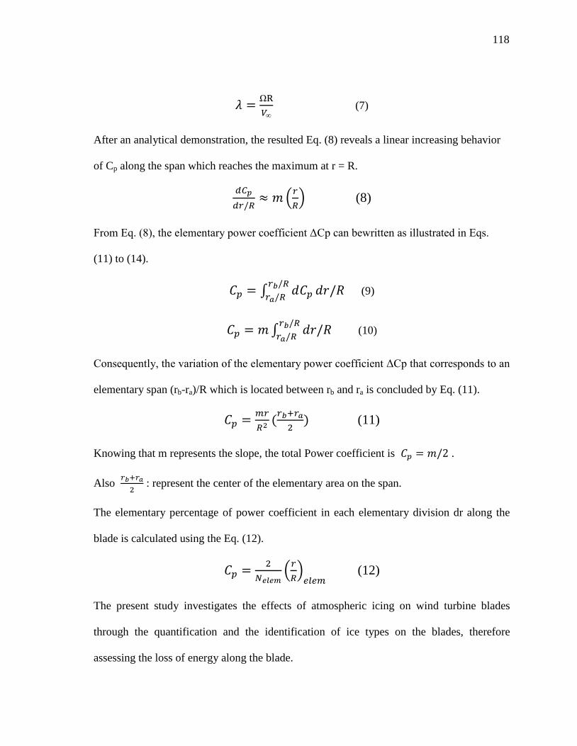
118

Ω

(7)

After an analytical demonstration, the resulted Eq. (8) reveals a linear increasing behavior

of Cp along the span which reaches the maximum at r = R.

(

) (8)

From Eq. (8), the elementary power coefficient ΔCp can bewritten as illustrated in Eqs.

(11) to (14).

∫

(9)

∫

(10)

Consequently, the variation of the elementary power coefficient ΔCp that corresponds to an

elementary span (rb-ra)/R which is located between rb and ra is concluded by Eq. (11).

(

) (11)

Knowing that m represents the slope, the total Power coefficient is .

Also

: represent the center of the elementary area on the span.

The elementary percentage of power coefficient in each elementary division dr along the

blade is calculated using the Eq. (12).

(

)

(12)

The present study investigates the effects of atmospheric icing on wind turbine blades

through the quantification and the identification of ice types on the blades, therefore

assessing the loss of energy along the blade.

119

3.5 Results

3.5.1 Power along the blade

The power production is proportional to wind speed which initiates the rotation of

the blades. The uneven distribution of relative velocity along the blade generates inconstant

elementary distribution of power. Using Eqs. (12) and (20), Figure 3.4 illustrates a linear

increase of power coefficient starting from the root of the blade to the tip. The power

generated from the first 20 % of the blade is almost neglected (~4 %), on the other hand the

last 20 % of the blade (36 %) generates the highest power. Furthermore, an approximate 85

% of the power is located in the last 60 % of the radial position of the blade. According to

Burton et al. (2001), at the tip of the blade the lift force is almost normal to the rotor plane.

The tangential component of the lift force is small and its contribution to the torque is

insufficient. Consequently the power is reduced at the tip of the blades.

Figure 3.4. Elementary power coefficient along the span

120

3.5.2 Water collection effeciency

According to Eq. (3), collection efficiency is an important factor that contributes in

controlling the amount of accreted ice. Therefore, within similar meteorological and

geometric conditions, hydrometeors with different subfreezing water droplet diameters

generate different collection efficiencies along the blade. Figure 3.5 shows three profiles of

collection efficiency that correspond to supercooled stratus clouds (fog), supercooled

drizzle and freezing rain with droplet diameters 20 μm, 200 μm and 2000 μm respectively.

Due to the large size of rain drops, the water drops are all collected when at impact with the

leading edge along the entire blade, as shown in Figure 3.5. Except for a slight decrease of

collection efficiency near the root of the blade, the drizzle droplets maintain a high

collection which is compared to that of rain droplets. Distinctively, supercooled fog

droplets with a diameter of 20 μm are characterized with a collection efficiency that varies

approximately from 0.09 near the root of the blade to more than 0.9 at the tip. Depending

on the radial position, the rotational motion of wind turbine leads to a linear increase of

relative velocity, starting from the root of the blade to the tip. The outer section of the blade

has the smallest chord length and leading edge. Furthermore, Figure. 5 corroborates the fact

(Eqs. (4)–(5)) that higher velocity, smaller water drops and cylinder diameter all increase

the droplet collection efficiency.

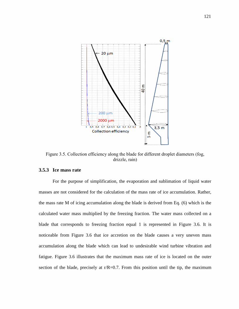
121

Figure 3.5. Collection efficiency along the blade for different droplet diameters (fog,

drizzle, rain)

3.5.3 Ice mass rate

For the purpose of simplification, the evaporation and sublimation of liquid water

masses are not considered for the calculation of the mass rate of ice accumulation. Rather,

the mass rate M of icing accumulation along the blade is derived from Eq. (6) which is the

calculated water mass multiplied by the freezing fraction. The water mass collected on a

blade that corresponds to freezing fraction equal 1 is represented in Figure 3.6. It is

noticeable from Figure 3.6 that ice accretion on the blade causes a very uneven mass

accumulation along the blade which can lead to undesirable wind turbine vibration and

fatigue. Figure 3.6 illustrates that the maximum mass rate of ice is located on the outer

section of the blade, precisely at r/R=0.7. From this position until the tip, the maximum

122

mass rate shows a slight decrease. Toward the opposite direction the maximum mass rate

decreases significantly to reach its minimumnear the blade root zone. Higher liquid water

content corresponds to higher accumulation mass rates and a more accentuated peak. The

highest ice accumulation rate shown in Figure 6 corresponds to the highest value of liquid

water content 0.36 g · m-3

followed by 0.2 g·m-3

, 0.07 g·m-3

and 0.04 g·m-3

respectively.

Figure 3.6. Ice mass rate along the span for different liquid water contents.

3.5.4 Aerodynamic effect

In order to investigate the aerodynamic effect of ice accumulation along the blade, a

dimensionless thickness rate is introduced. This parameter h/c is represented by the ratio of

thickness rate to chord length. The dimensionless thickness rate distribution on the blade

123

for four liquid water contents 0.04 g·m-3

, 0.07 g·m-3

, 0.2 g·m-3

, 0.36 g·m-3

is illustrated in

Figure 3.7. For different liquid water contents the thickness rate follows a similar tendency

as the collection efficiency that increases towards the tip of the blade. However the gradient

of thickness rate along the blade is less important for smaller values of liquid water content.

The area on the blade that is most affected aerodynamically due to ice accumulation is

located approximately on the last 20 % of the outer section of the blade.

Figure 3.7. Maximum ice thickness rate along the span for different liquid water content

The behavior of the dimensionless thickness h/c is illustrated in Figure 3.8, for a

liquid content of 0.2 g·m-3

at a wide range of subfreezing temperatures [0 °C -14 °C]. When

the temperature becomes colder than -14 °C, the dimensionless thickness reaches its

maximum limit and remains unchangeable. The increase of elementary power production

from the root to the tip of the blade illustrated in Figure 3.4 is corroborated by the same

124

tendency of the aerodynamic effect shown in Figure 3.8. In addition, within the same

position on the blade, the variation of subfreezing temperatures has an accentuated

aerodynamic impact towards the tip of the blade. Consequently, ice thickness appears most

pronounced along the blade where the most power is generated. An apparent inconsistency

regarding the effect of temperature along the blade is also featured in Figure 3.8. The

aerodynamic effect is insignificant at all temperatures near the root of the blade. On the

other hand, away from the root of the blade, colder temperatures manifest a larger

aerodynamic response.

Figure 3.8. Aerodynamic effect along the blade for LWC =0.2 g∙m-3

.

125

3.5.5 Freezing fraction

In order to determine the boundary values that distinguish the wet icing processes

(Glaze) from the dry icing processes (Rime), the Ludlam limit along the span for different

temperatures and four liquid water contents is plotted in Figure 3.9. This limit represents

the temperatures at which the liquid water becomes fully frozen and the freezing fraction

is equal to 1. Therefore, larger amounts of collected supercooled liquid water located at the

radial positions from r/R = 0.8 to the tip of the blade require the coldest temperature to

reach a complete solidification. Furthermore, the radial positions from r/R=0.8 to the tip are

characterized by a nearly similar freezing fraction. Under icing conditions with liquid water

contents 0.36 m·s-1

, 0.2 m·s-1

, 0.07 m·s-1

, and 0.04 m·s-1

and at air temperatures −23 °C,

−13.5 °C, −5 °C, and −3 °C respectively, all the collected water along the blade completely

freezes and forms rime ice. On the other hand, at higher temperature both rime ice and

glaze are formed on the blade, with rime ice near the root of the blade, followed by glaze on

the outer section of the blade.

126

Figure 3.9. Ludlam limit for different liquid water content.

The radial position of the transition point between Rime and Glaze depends on air

temperature. Freezing fractions at different temperatures are represented on Figure 3.10.

The freezing fraction which is equal to 1 reflects a complete freezing of liquid water and

therefore associated with rime ice. Within the subfreezing range, specifically at warmer

temperatures, the collected supercooled liquid water turns into rime ice, initially near the

root of the blade, while the other distant radial positions keep the supercooled liquid water

partially frozen (glaze). As shown in Figure 3.10, further cooling leads to an increase of

rime ice which will gradually cover the entire blade. In addition, the critical effect of air

temperature on freezing fraction and consequently the type of ice are demonstrated in

Figure 3.10. For a liquid water content of 0.2 g·m-3

and at air temperatures between 0 °C

and −2 ° C the collected liquid water is partially frozen and forms only glaze all over the

blade. With a temperature of supercooled liquid water at −2 °C and cooler, rime ice begins

127

to appear first in the inner section near to the root of the blade and moves progressively

with decreasing temperature towards the tip. Once the temperature reaches −13.5 °C, all the

collected water becomes frozen and forms rime ice all along the blade. Partial freezing of

the collected supercooled liquid water generates a runback of the unfrozen liquid water

which eventually will freeze and form uneven shapes of ice. The freezing fraction 0.88

represents a critical value that brings about the most aerodynamic hazardous double horn

ice shape (Fortin and Perron, 2009). For a liquid water content of 0.2 g·m-3

the temperature

−12 °C represents the coldest temperature that maintains a freezing fraction of 0.88 located

on the outer section of the blade r/R ~ [0.93 0.96].

Figure 3.10. Freezing fraction along the span for different temperatures (LWC = 0.2

g·m−3

).

128

3.5.6 Power loss

In the zone of interest on the blade which is located between the radial position

r/R=0.8 and 1, the power production represents 38% of the total production of awind

turbine. The supercooled liquid water collected in this segment of the blade requires the

coldest air temperature in order to form rime ice. Within this section, the accumulated glaze

on the blade reshapes the airfoil resulting in higher aerodynamic degradation. Decreasing

temperature as shown in Figs. 9 and 10 indicates that the radial position r/R ~ [0.93 0.96] is

the last position where collected water becomes rime ice on the blade. In order to quantify

production degradation, the power loss factor f is introduced. The values of the power loss

factor f reflect the normalized variations of power requirements for rotor blade helicopters

under icing conditions.

′

𝑓 (13)

Cp’ represents power coefficient under icing effect and f is derived from the effect of ice

on helicopter power requirements introduced by Fortin and Perron (2009). Contrary to

helicopters that require power to rotate, wind turbines rotate to produce power. For rotating

iced blade of helicopter it requires an increase of the provided power to maintain the

rotation frequency. On the other hand, ice accumulation on wind turbines reduces the

expected power production. Therefore the power coefficient for clean wind turbine blades

is divided by the power loss factor f in order to obtain the power coefficient under icing

conditions. The power loss factor f, as shown in Figure 3.11a and 3.11b, reflects the

aerodynamic degradation and power loss which depends on the freezing fraction that

129

determines the ice shape. This factor intervenes only at subfreezing temperatures starting

with a value 1 at 0 °C which corresponds to a clean blade. Beyond a value of 1, the power

loss factor f follows a linear increase until it reaches its maximum value at 4.4. This peak

value is associated with the freezing fraction 0.88 that corresponds to the double horn ice

shape which is the most aerodynamically hazardous situation. Further cooling is associated

with an increase in freezing fraction and a slight decrease of the power loss factor f until it

reaches the minimum value of 3.3. At this minimum, the freezing fraction is equal to 1 and

all the supercooled liquid water becomes fully frozen and forms rime ice. The power loss

factor that indicates the maximum energy degradation at the radial position r/R ~[0.93:0.96]

is accordingly applicable for all liquid water contents. Figure 3.11b illustrates power loss

factor for liquid water contents of 0.04 g·m−3

, 0.07 g·m−3

, 0.2 g·m−3

, and 0.36 g·m−3

that

corresponds to the maximum aerodynamic degradation at temperatures −2.6 °C, −4.5 °C,

−12 °C, and −20 °C respectively, and forming rime ice at temperatures −3 °C, −5 °C, −13.5

°C, and −23 °C respectively. According to the variation of power loss factor in Figure

3.11b, the higher liquid water contents are featured with larger ranges of temperatures

where the power loss caused by glaze is significant. The radial position r/R ~ [0.93:0.96]

that belongs to the outer section of the blade brings about the largest power production.

130

Figure 3.11. Aerodynamic reduction factor (a) Power loss vs freezing fraction (b) Power

loss vs temperature for different liquid water contents.

Simultaneously, the freezing fraction 0.88 is associated with the double horn ice shape that

imposes the highest aerodynamic degradation. For these reasons, Figure 3.12 shows how a

particular focus on power production is achieved within these conditions. The degradation

of elementary power coefficient Cp versus the temperature at the radial position r/R ~

[0.93:0.96], for four values of liquid water contents; 0.04, 0.07, 0.2, and 0.36 g·m−3

is

131

shown in Figure 3.12. Power coefficient decreases with decreasing temperature until it

reaches its lower limit that corresponds to the critical freezing fraction of 0.88, then it

increases slightly to reach a constant value to form rime icewhen the freezing fraction is

equal to 1. With liquid water content 0.2 g·m−3

, one notices that power production

decreases until its minimum that corresponds to temperature −12 °C and a freezing fraction

0.88. Colder than −12 °C, freezing fraction increases and it generates a slight increase in

power until reaching a freezing fraction 1 when at which point the dry growth regime starts.

The depletion of power coefficient in Figure 3.12 is reached only if enough ice is

accumulated on the blade. Also, the behavior of power coefficient in Figure 3.12 pictures

shows the response of wind turbine production loss to geometrical and meteorological icing

conditions. For this calculation it is assumed that the icing event duration is long enough to

generate the critical ice shape. The upper half of the blade is more affected by icing due to

the partial freezing. With regard to liquid water content of 0.2 g·m−3

and a temperature of

−12 °C, the power degradation appears under all icing types (rime and glaze). As shown in

previous Figure 3.10, starting from a radial position near r/R = 0.72 that corresponds to the

beginning of glaze, the magnitude of power degradation increases gradually and becomes

more accentuated. At its lower level it is located approximately at r/R ~ [0.93 0.96]. The

amount of accumulated ice depends on the duration of ice accretion.

132

Figure 3.12. Power loss at r/R ~ [0.93 0.96] for different liquid water contents.

According to Fortin and Perron (2009), the highest power loss for the subscaled iced

helicopter's blades was reached after 160 s of ice accretion, the relative speed of the blade

at the radial position r/R ~ [0.93 0.96] was about 130 m·s−1

and a liquidwater content of

0.84 g·m−3

. Accumulation parameter A presented in Eq. (14) (Anderson and Tsao, 2005) is

utilized, in order to estimate the duration required for ice accretion on wind turbine blades

to reach a similar ice shape (hazardous double horn).

(14)

A: Accumulation parameter, E: total collection efficiency, U: relative speed, t: icing event

duration, C: chord. The indexes wt, h refer to wind turbine and helicopter respectively. For

the same freezing fractions, collection efficiencies and accumulation parameters (Awt, Ah),

133

the duration required for ice accretion on the blade of a turbine is represented in Eq. (15)

and Figure 3.13 that correspond to different liquid water contents:

(15)

Higher liquid water contents correspond to shorter required icing duration to reach higher

power loss. In reference to the subscaled helicopter's rotor blade (Fortin and Perron, 2009),

Figure 3.13 illustrates the required duration for ice accretion on wind turbines to match the

same or the highest power loss under icing conditions on the helicopter's blades (freezing

fraction 0.88, r/R= [0.93 0.96]) for different liquid water contents. As illustrated in Figure

3.13, for liquid water contents 0.04 g·m−3

, 0.07 g·m−3

, 0.2 g·m−3

, and 0.36 g·m−3

the

durations needed to reach the hazardous double horn ice shapes are 13.2 h, 7.5 h, 2.6 h and

1.5 h respectively. In addition, icing events with liquid water contents smaller than 0.04

g·m−3

are excluded from forming double horn ice shapes with a freezing fraction of 0.88. In

order to evaluate the required duration of icing events, the results from Figure 3.13 are

compared to realistic icing events.

134

Figure 3.13. Required duration for ice accretion on wind turbines to match the same

highest power loss under icing conditions on helicopter's blades (freezing fraction 0.88,

r/R= [0.93 0.96]) for different liquid water contents.

The use of North American Regional Reanalysis (NARR) allowed a climate

investigation of in-cloud icing near surface level, during a 32 year period from 1979 until

2010. As shown in Figure 3.14, from these reanalysis over the site of Mount-Bélair

(Canada), the duration of icing events and the corresponding supercooled liquid water

contents are estimated according to a previous study done by Lamraoui et al. (2013). The

calculation of the 32-year average that corresponds to the occurrence of icing events

enables finding the typical durations for each range of supercooled liquid water contents of

0.04 ± 0.02 g·m−3

, 0.07 ± 0.02 g·m−3

, 0.2 ± 0.02 g·m−3

, and 0.36 ± 0.02 g·m−3

. The longer

durations of icing event are associatedwith a smaller supercooled liquid water contents.

135

Figure 3.14. Monthly duration of icing events from reanalysis over Mount-Bélair site

during January (from 1979 to 2010).

The 32-year averages of the duration of icing events are introduced in Table 3.1. The

results demonstrated in Table 3.1 characterize the climatology of atmospheric icing of the

Mount-Bélair site located near Quebec City (Canada).

Table 3.1 : Duration of icing events from reanalysis: 32-year icing climate

The values of liquid water contents in Figure 3.14 and Table 3.1 delineate five

severity classes (Lamraoui et al., 2013). The comparison of icing event durations from

Figure 3.13 and Table 3.1 shows that all icing severity ranges endure enough to fulfill the

136

requirement of forming the double horn hazardous ice shape. The freezing fraction of 0.88

corresponds to the largest aerodynamic degradation. Therefore, the starting temperature that

coincideswith the occurrence of ice accretion along the blade with freezing fraction only

0.88 and beyond corresponds to the maximum power loss. For a liquid water content 0.2 g ·

m-3

, the maximum power loss happens at temperature −12 °C. Under these meteorological

conditions, the radial position r/R~[0.93 0.96] holds an ice with a freezing fraction of 0.88.

Elsewhere on the blade the freezing fraction exceeds 0.88 and varies accordinglyto reach 1.

The electrical power loss due to icing conditions is represented in Figure 3.15. The

maximum electric power degradation that wind turbines can reach under icing effects is

obtained by involving the modified power coefficient Cp′ from Eq. (13). More specifically,

Figure 3.15(b) represents the quantification of power loss for different wind speed when the

liquidwater content is 0.2 g·m−3

and air temperature equivalent to −12 °C. Under these

geometrical and meteorological conditions, the maximum power production loss occurs

when wind speed is approximately around 10.5 m·s−1

. At the temperature of −13.5 °C, only

rime ice is accreted all along the blade, showing power degradation. The temperature of

−12 °C engenders only rime ice on the radial positions from the root until r/R ~ 0.72.

Beyond this position to the tip of the blade, only glaze is accreted with a different freezing

fraction. From the result represented in Figure 3.15, one concludes that a slight change in

temperature can provoke a change in power loss. Within a range of wind speed ~ [7 m·s−1

17 m·s−1

], a small decrease in temperature (ΔT ~ 1.5 °C) generates a significant reduction

of power production that can reach its maximum of 0.8% with a wind speed of 10.5 m·s−1

.

137

Under icing conditions, both temperatures −12 °C and −13.5 °C correspond to significant

maximumpower production degradation of approximately 40%.

Figure 3.15. Power under icing effects for LWC = 0.2 g · m−3 at T = −12 °C and T = −13.5

°C, (a) Power curve with and without icing (b) Electrical power loss.

138

3.6 Analysis

Since the rotational motion of the blade generates a varying relative velocity that

increase from zero at the root of the blade to itsmaximum at the tip, consequently the

elementary power is distributed unevenly along the blade. The power production extracted

from the first quarter of the blade near the root is practically neglected. Except for the tip,

the blade aerodynamic is greatly influenced by the outer section. The obtained result as

shown in Figure 3.4, demonstrates that 85% of the produced power is originated from the

outer 60% segment of the blade. From the simplified cylinder model used in this study, the

collection efficiency involved in quantifying ice accretion varies mainly according cylinder

diameter, and droplet diameter of supercooled hydrometeors. Considering all ranges of

supercooled hydrometeors, with larger droplet diameters (≥200 μm) that are associated with

freezing drizzle or rain, the collection efficiency is approximately consistent and not

affected by the geometry variation along the blade. On the other hand, as illustrated in

Figure 3.5 supercooled fog or supercooled cloud has a substantial variation of collection

efficiency between both edges of the blade. The outer section of the blade that coincides

with a higher aerodynamic is characterized with the highest collection efficiency that is

comparable to freezing rain or drizzle.

The rate of ice thickness and the rate of the ratio of thickness to chord as show in

Figures 3.7 and 3.8 respectively corroborate the fact that the outer section of the blade

considerably influence the aerodynamics of the blade and is the least ice-phobic segment on

the blade.

139

The freezing faction is a very important parameter that substantially influences the

type and the shape of accreted ice on the blade. As illustrated in Figure 3.9, the fact that

higher liquid water contents associated with higher latent heat requires colder temperature

to reach the complete solidification of collected supercooled liquid water. When

temperature decreases as indicated in Figures 3.9 and 3.10, rime ice starts to appear first

near the root then gradually continues to spread towards the tip of the blade.

Blade's airfoils are sensitively designed to allow a smooth flow of air over the top

and bottom surfaces and when ice accumulation occurs it then alters the shape of airfoil.

The geometry of a blade's airfoil is crucial to the aerodynamics of wind turbines and

consequently for power production. Rime ice follows the shape of the airfoil; however the

glaze shape can be very irregular depending upon the freezing fraction. When ice first

accumulates it has no serious effect, but gradually it builds forward and along the top and

bottom surfaces of airfoil and causes more hazard. When the blade of a wind turbine strikes

supercooled water droplets, the leading edge becomes covered with a film of supercooled

water that freezes from inside out. Clear ice (glaze) which forms rapidly can represent the

most hazardous form of all icing conditions, whereas rime ice forms slowly. At the

beginning, the ice build-up follows the blade's airfoil. Once it reaches the points of

maximum camber, the shape of airfoil changes drastically. Consequently the air flow

becomes disrupted which generates drag increase, and reduced lift. From an experimental

study (Fortin and Perron, 2009) the freezing fraction of 0.88 is proven to generate the most

aerodynamically hazardous ice shape (double horn). This freezing fraction and a

normalized power variation from a helicopter's rotor blade were used to introduce a new

140

power loss factor to assess power degradation subjected to ice accretion. This power loss

factor is introduced in Figures 3.11a and 3.11b. For each elementary radial position along

the blade, the freezing fraction zero corresponds to no-ice condition. The collected

supercooled liquid water starts to freeze with increasing freezing fraction and decreasing

the temperature until reaching the peak of power loss that corresponds to the freezing

fraction of 0.88. As shown in Figure 3.11b, the temperature required to reach the maximum

loss varies according to the value of liquid water content. Once the maximum power loss is

achieved, an additional cooling will generate lesser power loss. Radial position of r/R ~

[0.93 0.96] corresponds to the most critical freezing fraction on the blade.

Under the same meteorological conditions, the critical zone on the blade is limited

to a small section where potentially the double horn ice shape would form with a freezing

fraction of 0.88. Therefore, Figure 3.12 demonstrates power degradation of the critical

temperatures for 4 values of liquid water contents 0.04 g·m−3

, 0.07 g·m−3

, 0.2 g·m−3

, and

0.36 g·m−3

. By matching the accumulation parameters from a subscaled helicopter rotor

blade with wind turbine blade helps determine the required duration of icing events that

leads to the formation of the double horn ice shape. The variation of this recommended

duration is presented in Figure 3.13. Within the range of liquid water content used for this

study, the duration of icing events needed to form a double horn ice shape varies between

1.5 h and 13 h. As an attempt to verify whether these critical durations correspond to

realistic icing events, the current study refers to a reliable set of historical meteorological

database details from the North American Regional Reanalysis (NARR).

141

The analysis of data from North American Regional Reanalysis at a climate scale

that spanned 32 years during January demonstrated that less intense icing events had

smaller liquid water content and were associated with prolonged occurrences of icing

events. During very intense icing events with a short period of occurrences, the optimum

alternative for wind turbines is to stop turning, in order to minimize ice accumulation. The

results obtained from reanalysis in Table 3.1 demonstrate that intense icing events last up to

6 h. On the other hand, light icing events that can exceed 2 days, this can present prolonged

power degradation and serious hazardous conditions for the wind turbine industry. In

addition, Figure 3.5 illustrates that smaller droplets target the most aerodynamically critical

zone on the blade which is located in the outer section. Therefore, shorter occurrences of

icing events that correspond to higher intensity with larger droplet diameters are less

harmful.

The critical freezing fraction 0.88 that corresponds to the double horn ice shape

occurs locally within a limited segment on the blade. Once freezing fractions along the

blade reaches 0.88 or higher, the wind turbine indicates the maximum of power

degradation. This scenario corresponds to glaze accumulation located on r/R ~ [0.93 0.96]

and rime ice elsewhere on the blade. The power output shown in Fig. 15 which originated

from clean and iced blades reveal that regardless of the type of ice, the power production

degradation is still significant and can reach ~40 % of the expected power production. The

critical glaze contributes slightly to power loss with an approximate amount of ~0.8 %,

because of the limited area where the double horn ice shape forms in relation to the entire

blade.

142

3.7 Conclusion

The present study determines power production loss, due to the accumulation of ice

along the blades of wind turbines. The investigation is based on cylinder model and power

loss model. The power degradation model is based on the results of a previous study that

was done on a sub-scaled helicopter rotor blade. The approach depends on the assumption

that a wind turbine remains continually operational, regardless the severity of icing events.

Along the blade, the results show that both mass and thickness of accreted ice on the

leading edge increase gradually with decreasing the chord size. The results show that 85%

of power production is generated from the section on the blade that is located in the last

60% of the blade towards the tip. As well, the results enable the identification of the

localized radial position that starts from r/R=0.8 to the tip of the blade and corresponds to

the highest aerodynamic degradation and consequently power production loss. According

to the size of the leading edge, the air temperature, the liquid water content and the freezing

fraction vary along the blade resulting in different ice types and shapes. Regardless of the

type of ice, power production loss under icing conditions can reach a maximum of 40 % at

a specific wind speed. Locally and within the same radial position, it is the shape rather

than the thickness of ice that causes more icing hazards. The double horn shaped ice

propels the highest aerodynamic degradation. This ice geometry corresponds to the freezing

fraction of 0.88. In addition, from power loss model, the peak of the local power loss is

associated with freezing fraction of 0.88 which represents only a portion of wet growth

regime. The coexistence of both wet and dry ice simultaneously on the blade, and the

limited radial section that has a critical freezing fraction, minimize the effect of local

143

double horn shaped ice formation and of power production loss on the entire from the

whole wind turbine. Therefore, there is only a slight difference of approximately 0.8% in

total power production loss caused by the existence of a confined critical wet ice along the

blade, when compared to only dry ice. Typical icing event durations at climate scale

obtained from reanalysis confirm that all icing events with all intensities persist enough to

reach the hazardous freezing fraction. Also, icing events with high intensities correspond to

shorter durations of occurrence. On the other hand, less intense icing events had smaller

liquid water content and were associated with prolonged occurrences of icing events; light

intensities events are associated to long lasting icing events. Based on the obtained results

of this study, it can be useful to set up a cost effective ice-protection system. Regarding this

system, it is recommended to cover only 60% of the blade. Thiswould optimize power

production under icing conditions. Also, this systemcan be equipped with a sensor located

at the radial position r/R=0.4 or higher toward the tip. This sensor can then trigger the ice-

protection system upon detection of a critical freezing fraction at this radial position.

144

3.8 References

Abbot, I., von Doenhoff, A., 1959. Theory of wing sections, 2nd edition. Dover

Publications, New York.

Anderson, D.N., Tsao, J.C., January 6–9, 2003. Evaluation and validation of the messenger

freezing fraction. AIAA–2003–1218 41st Aerospace Sciences Meeting and Exhibit.

American Institute of Aeronautics and Astronautics, Reno, Nevada.

Antikainen, P., Peuranen, S., 2000. Ice loads, case study. BOREAS V, wind power

production in cold climates. Proceedings of an International conference, Levi, Finland.

Finnish Meteorological Institute (CD-ROM).

Bendix, J., Thies, B., Cermak, J., Nauß, T., 2005. Ground fog detection from space based

on MODIS daytime data — a feasibility study. Weather Forecast. 20, 989–1005.

Bose, N., Rong, J.Q., 1990. Power reduction from ice accretion on a horizontal axis wind

turbine. Proc.12th British Wind Energy Association, Wind Energy Conference Norwich,

UK.

Botta, G., Cavaliere, M., Holttinen, H., 1998. Ice accretion at Acqua Spruzza and its effects

on wind turbine operation and loss of energy production. BOREAS IVFMI, Hetta, Finland

77–86.

Brodkey, R.S., Hershey, H.C., 1988. Transport phenomena: a unified

approach.McGrawInternational Edition, New York (847 pp).

Burton, T., Sharpe, D., Jenkins, N., Bossanyi, E., 2001. Wind Energy Handbook.

JohnWiley & Sons LTD. ISBN: 0-471-48997-2.

Cober, S.G., Isaac, G.A., Strapp, J.W., 1995. Aircraft icingmeasurements in east coast

winter storms. J. Appl. Meteorol. 34, 88–100.

Modelling the risk of icing. In: Dierer, S., Cattin, R., Muller, S., Nygaard, B., Steiner, P.,

Calpini, B. (Eds.), International workshop on Atmospheric Icing of Structures (IWAIS

XIII), Andermatt, September 8–11, 2009 (COST Action 727).

Fikke, S., Ronsten, G., Heimo, A., Kunz, S., Ostrozlik, M., Persson, P.E., Sabata, J.,

Wareing, B., Wichura, B., Chun, J., Laakso, T., Santti, K., Makkonen, L., 2006. 2006:

COST-727: atmospheric icing on structures measurements and data collection on icing:

state of the art. MeteoSwiss, Switzerland.

Fortin, G., Perron, J., 2009. Spinning Rotor Blade Tests in Icing Wind Tunnel. Paper AIAA

2009–4260 1st AIAA Atmospheric and Space Environments Conference, San Antonio, TX.

145

Fortin, G., Perron, J., Ilinca, A., October 2005. A study of icing events at Murdochville:

conclusions for the wind power industry. International Symposium “Wind Energy in

Remote Regions”, Magdalen's Island.

Hansen, M.O.L., 2008. Aerodynamics ofwind turbines, Earthscan, London (UK) and

Sterling (USA) 2nd edition. 181.

Hochart, C., Fortin, G., Perron, J., Ilinica, A., 2008. Wind turbine performance under icing

conditions. Wind Energy 11, 319–333.

Isaac, G.A., 1991. Microphysical characteristics of Canadian Atlantic storms. Atmos.

Res.26, 339–360.

Jacobs, E.N., 1932. Airfoil section characteristics as affected by protuberances. NACA

Report No. 446.

Jasinski, W.J., Noe, S.C., Selig, M.S., Bragg, M.B., 1998. Wind turbine performance under

icing conditions. J. Sol. Energy Eng. 120, 60–65.

Jones, R.,Williams, D.H., 1936. The effect of surface roughness of the characteristics of the

aerofoils NACA 0012 and RAF 34. British ARC, R&M No. 1708.

Laakso, T., Peltola, E., 2005. Review on blade heating technology and future prospects.

2005 BOREAS VII Conference, 7–8th March 2005, Saarislkä, Finland.

Laakso, T., Baring-Gould, I., Durstewitz, M., Horbaty, R., Lacroix, A., Peltola, E.,

Ronsten, G., Tallhaug, L., Wallenius, T., 2010. State-of-the-art of wind energy in cold

climates. VTT Working Papers 152. VTT Technical Research Centre of Finland (71 pp.).

Laforte, J.-L., Allaire, M.A., 1992. Évaluation du Givromètre d'Hydro-Québec à

Différentes Intensités de Givrage Sec et Humide. Rapport HQ-92-02.

Lamraoui, F., Fortin, G., Benoit, R., Perron, J., Masson, C., 2013. Atmospheric icing

severity: quantification and mapping. Atmos. Res. 128, 57–75.

Makkonen, L., Autti, M., 1991. The effects of icing on wind turbines. EWEC, Amsterdam,

Netherlands. 575–580.

Manwell, J.F., McGowan, J.G., Rogers, A.L., 2009. Wind energy explained: theory, design

and application. John Wiley & Sons 424.

Marjaniemi,M., Peltola, E., 1998. Blade Heating Element Design and Practical

Experiences. BOREAS IVFMI, Hetta, Finland 197–209.

146

Mazin, I.P., Korolev, A.V., Heymsfield, A., Isaac, G.A., Cober, S.G., 2001.

Thermodynamics of icing cylinder for measurements of liquid water content in supercooled

clouds. J. Atmos. Ocean. Technol. 18, 543–558.

Messinger, B.L., 1953. Equilibrium temperature of an unheated icing surface as a function

of air speed. J. Aerosol Sci. 29–42 (vol. Jan).

Parent, O., Ilinca, A., 2011. Anti-icing and de-icing techniques for wind turbines. Crit.

Rev.Cold Reg. Sci. Technol. 65, 88–96.

Seifert, H.,Westerhellweg, A., Kröning, J., 2003. Risk analysis of ice thrown fromwind

turbines. BOREAS VI conference, April 2003, Pyhä, Finland.

Tammelin, B., Säntti, K., 1996. Estimation of Rime Accretion at High Altitudes —

Preliminary Results. BOREAS IIIFMI, Saariselkä, Finland 194–210.

Tammelin, B., Säntti, K., 1998. Icing in Europe. BOREAS IVFMI, Hetta, Finland 125–132.

Vestas, 2006. Wind turbine product descriptions V80-1.8 MW. Vestas Americas Inc.

vestas.com.

Walton, W.H., Woolcock, A., 1960. The suppression of airborne dust by water spray. Int. J.

Air Pollut. 3, 129–153.

GENERAL CONCLUSION

The present thesis brings together the important results and the acquired scientific

knowledge during my doctorate studies that yielded three original research articles.

There is the need for an anticipated knowledge of icing occurrences in a given area

prior implanting ice-sensitive structures. The uncertainty with respect to the occurrence of

icing events motivated many experimental and modeling studies including the current

thesis to investigate the historical and real-time characteristics of icing events.

The assessment of the icing severity in this thesis has two stages that accommodate the

topographic irregularity and the calculation cost involved. The first stage focuses on using

coarse resolution data spanning a long time period, in order to preliminary identify large

regions with high icing severity. The second stage focuses on identifying icing events over

complex terrains with mountainous and localized irregular topography, which involves

numerical simulations with the use of the mesoscale weather model «GEM-LAM» (Global

Environmental Multiscale - Limited Area Model), equipped with the sophisticated

microphysics scheme Milbrandt and Yau.

Based on cylinder model for ice accretion, the climatology of atmospheric icing is

introduced using an unprecedented long representation of icing events spanning a 32-year

dataset of meteorological variables from North American Regional Reanalysis. The

proposed icing severity index that assesses the severity of icing events consists of three

weighting factors that reflect the severity classes, the duration of icing events and the liquid

water content. Subsequently, an updated version of in-cloud icing climatology at high

148

resolution is achieved using double-nested GEM-LAM simulations driven by NARR. Due

to the time consuming numerical calculations, a hybrid approach is used to combine

numerical model icing calculations during significant icing days from GEM-LAM and

icing calculations during non-significant icing days obtained from NARR. In addition,

through an investigation of high resolution output, the interrelationships between

meteorological icing key parameters were revealed and 3D near-surface icing climatology

is identified. The end product of the studies in chapter 1 and chapter 2 represents the

climatology of icing severity over a 15-year period at high resolution. The proof-of-concept

of the hybrid methodology presented for the Quebec region could be easily adapted to other

cold areas (or cold season months) of the world to obtain their icing severity index maps.

With regards to the impact of atmospheric icing on wind turbines, this Thesis

investigated the effect of the phase and the size of cloud droplets on collection efficiency

and freezing fraction. In addition typical values of the duration of icing events were

introduced for different liquid water contents. The results obtained can help the setup of a

sensor that triggers the ice-protection system upon detection of the critical freezing fraction.

The methodology used in this dissertation permitted the achievement of the

objectives that were initially planned with regard to the climatology of in-cloud icing

events using reanalysis and an optimal high resolution hybrid approach of mesoscale

modeling. In addition to the advantage of high resolution mesoscale modeling compared to

the coarse resolution of NARR, GEM-LAM showed the ability of identifying the vertical

profile of the characteristics of icing events at different altitudes above ground level.

149

Finally, with the use of the power loss factor indicated in chapter three and key

meteorological parameters for icing events originated from NARR, GEM-LAM or other

sources will enable the evaluation of wind turbine power degradation.