POLITECNICO DI MILANO

SCUOLA DI INGEGNERIA INDUSTRIALE E DELL'INFORMAZIONE

Corso di Laurea Magistrale in Ingegneria Matematica

TESI DI LAUREA MAGISTRALE

A Bayesian analysis of population density over

time:

how spatial correlation matters

Relatore: Dott.ssa Ilenia Epifani

Correlatore: Prof.ssa Alessandra Guglielmi Candidato:

Chiara Ghiringhelli

Matr. 823392

Anno Accademico 2015 - 2016

Abstract

In this work we propose a dynamic Bayesian approach to modeling the population's

density; predictors of dierent nature are used, e.g. economics and geographic indices.

The model is applied to the evaluation of the location of population in the state of Mas-

sachusetts over a period of 50 years, from 1970 to 2010. The aim of this work is to

introduce into the analysis both spatial and time correlation among data. We deal with

AutoRegressive models, that provide the most common way to explore time dependence.

In order to explore spatial correlation, we propose two dierent generalized regression

mixed models: one with spatial independent random eects and one that includes spa-

tial random eects evolving as a Conditionally AutoRegressive model (CAR). Both are

compared with a baseline linear model. For the CAR model, we derive the analytical

expression of the full conditional distributions necessary to build a MCMC algorithm

eciently coded in Julia language, and to sample from a posterior distribution. The

implementation of the other two models were made in Stan.

Keywords: Areal data models; AutoRegressive model; Bayesian analysis; CAR;

MCMC algorithm; Spatial random eects.

i

ii

Sommario

In questo lavoro proponiamo un approccio dinamico bayesiano per modelizzare la den-

sità di popolazione; vengono utilizzati predittori di diversa natura, per esempio indici

economici e geograci. Il modello è applicato all'evoluzione dello stanziamento della

popolazione nello stato del Massachusetts lungo un periodo di 50 anni, dal 1970 al 2010.

Lo scopo del lavoro è di introdurre nell'analisi una correlazione spaziale e una temporale

tra i dati. Utilizziamo un modello autoregressivo, che è uno degli strumenti fondamen-

tali per esplorare la correlazione temporale. Per quanto riguarda la correlazione spaziale,

proponiamo due modelli di regressione mista generalizzati: uno con eetti spaziali casuali

independenti e uno che include eetti spaziali che evolvono come un modello Condizion-

atamente Autoregressivo (CAR). Entrambi sono confrontati con un modello di riferi-

mento lineare. Per il modello CAR , calcoliamo l'espressione analitica delle distribuzioni

full conditional necessarie per implementare un algoritmo MCMC eciente e campionare

dalla distribuzione a posteriori. Abbiamo implementato l'algoritmo nel linguaggio di pro-

grammazione Julia. Mentre l'implementazionde degli altri due modelli è stata eettuata

in Stan.

Keywords:algoritmi MCMC; Analisi Bayesiana; Eetti spaziali casuali; Dati Spaziali;

modelli AutoRegressivi; modelli CAR.

iii

iv

Contents

1 Areal data models 5

1.1 Introduction of spacial correlation . . . . . . . . . . . . . . . . . . . . . . . 6

1.2 Measures of spatial association . . . . . . . . . . . . . . . . . . . . . . . . 7

1.3 Calculation of the joint distribution . . . . . . . . . . . . . . . . . . . . . . 9

1.3.1 Bayesian method . . . . . . . . . . . . . . . . . . . . . . . . . . . . 9

1.3.2 Existence and uniqueness of the joint distribution . . . . . . . . . . 11

1.4 Conditionally Autoregressive Models (CAR) . . . . . . . . . . . . . . . . . 15

1.4.1 Introduction of spatial random eects . . . . . . . . . . . . . . . . 17

2 Time series 19

2.1 Autoregressive Models . . . . . . . . . . . . . . . . . . . . . . . . . . . . . 21

2.1.1 Stationarity for AR models . . . . . . . . . . . . . . . . . . . . . . 22

2.1.2 Autocorrelation structure and Partial Autocorrelation Function . . 22

2.1.3 Bayesian inference for AR models . . . . . . . . . . . . . . . . . . . 23

3 A model for the population density 27

3.1 The data . . . . . . . . . . . . . . . . . . . . . . . . . . . . . . . . . . . . . 27

3.2 Descriptive statistic . . . . . . . . . . . . . . . . . . . . . . . . . . . . . . . 31

3.3 The model . . . . . . . . . . . . . . . . . . . . . . . . . . . . . . . . . . . . 38

3.4 Computational strategy . . . . . . . . . . . . . . . . . . . . . . . . . . . . 44

3.4.1 Gibbs Sampler . . . . . . . . . . . . . . . . . . . . . . . . . . . . . 44

3.4.2 Implementation with Stan and Julia . . . . . . . . . . . . . . . . . 49

v

4 Application to Massachusettes census tracts data 51

4.1 Posterior inference on the regression coecients . . . . . . . . . . . . . . 51

4.2 Autocorrelation and heteroschedasticity . . . . . . . . . . . . . . . . . . . 54

4.3 Models comparison . . . . . . . . . . . . . . . . . . . . . . . . . . . . . . . 65

5 Concluding Remarks 69

Appendices 71

A Full conditionals calculation 73

B Implementation codes 81

C Tables of the posterior quantiles of the regression coecients 91

D Convergence diagnostic of MCMC chains 95

Bibliography 98

vi

List of Figures

1.1 Example of dierent denition of distance for a regular grid. . . . . . . . 6

1.2 Example of a graph. . . . . . . . . . . . . . . . . . . . . . . . . . . . . . . 12

1.3 Example of clique: the subset 0, 1, 3, 4 is a clique because all the nodes

are connected. . . . . . . . . . . . . . . . . . . . . . . . . . . . . . . . . . 13

2.1 Example of PACF function: the value of the coecients are non inuential

after the rst time, so the correct order for this data set is p=1. . . . . . 23

3.1 Massachussettes state. . . . . . . . . . . . . . . . . . . . . . . . . . . . . . 28

3.2 Evolution of the mean of ppopulation log-density for every county during

the year 1970 (t=1), 1980 (t=2), 1990 (t=3), 2000 (t=4), 2010 (t=5). No-

tice that data in Barnstable, Franklin, Dukes, Nantucket are not collected

in 1970 and 1980 (see Table 3.1) . . . . . . . . . . . . . . . . . . . . . . . 31

3.3 Distribution of population density per year: in general the density is quite

small over time. . . . . . . . . . . . . . . . . . . . . . . . . . . . . . . . . . 34

3.4 Graph of population's log-density and distance per year. . . . . . . . . . . 34

3.5 Map of census tracts in Massachusettes in 1970. . . . . . . . . . . . . . . . 36

3.6 Map of census tracts in Massachusettes in 2010. . . . . . . . . . . . . . . . 37

4.1 Credibility intervals for the regression coecients at level 90%, under the

baseline model. . . . . . . . . . . . . . . . . . . . . . . . . . . . . . . . . . 52

4.2 Credibility intervals for the regression coecients at level 90%, under the

independent random eects model. . . . . . . . . . . . . . . . . . . . . . . 53

vii

4.3 Credibility intervals for the regression coecients at level 90%, under the

CAR model. . . . . . . . . . . . . . . . . . . . . . . . . . . . . . . . . . . . 53

4.4 Credibility intervals of the variances of the density population Y on log

scale at level 90%, under the baseline model. . . . . . . . . . . . . . . . . . 56

4.5 Credibility intervals of the variances of the density population Y on log

scale at level 90%, under the random independent eects model. . . . . . . 57

4.6 Credibility intervals of the variances of the density population Y on log

scale at level 90%, under the CAR model. . . . . . . . . . . . . . . . . . . 57

4.7 Estimation of the independent spatial random eects in 1970. . . . . . . . 58

4.8 Estimation of the independent spatial random eects in 1980. . . . . . . . 59

4.9 Estimation of the indipendt spatial random eects in 1990. . . . . . . . . 59

4.10 Estimation of the indipendt spatial random eects in 2000. . . . . . . . . 60

4.11 Estimation of the indipendt spatial random eects in 2010. . . . . . . . . 60

4.12 Estimation of the spatial random eects under the CAR model in 1970. . 61

4.13 Estimation of the spatial random eects under the CAR model in 1980. . 62

4.14 Estimation of spatial random eects under the CAR model in 1990. . . . . 62

4.15 Estimation of spatial random eects under the CAR model in 2000. . . . . 63

4.16 Estimation of the spatial random eects under the CAR model in 2010. . 63

4.17 Credibility intervals of the common term λ(t) in the variances of the spatial

random eects model at level 90%, under the random independent eects

model. Credibility intervals of the common term τ (t) in the variances of

the spatial random eects at level 90%, under the random CAR model. . 64

4.18 Predicted and actual log-density of population in 2010 under independet

random eects model. . . . . . . . . . . . . . . . . . . . . . . . . . . . . . 67

4.19 Predicted and actual log-density of population in 2010 under CAR model. 68

D.1 Traceplot and autocorrelation for the distance regressor under the CAR

model. . . . . . . . . . . . . . . . . . . . . . . . . . . . . . . . . . . . . . 95

D.2 Traceplot and autocorrelation for τ under the CAR model. . . . . . . . . 96

D.3 Traceplot and autocorrelation for ρ under the CAR model. . . . . . . . . 96

viii

D.4 Geweke test for the distance regressor under the CAR model in 1970, 1980,

1990, 2000 and 2010. . . . . . . . . . . . . . . . . . . . . . . . . . . . . . 97

D.5 Geweke test for τ under the CAR model in 1970, 1980, 1990, 2000 and

2010. . . . . . . . . . . . . . . . . . . . . . . . . . . . . . . . . . . . . . . 97

D.6 Geweke test for ρ under the CAR model in 1970, 1980, 1990, 2000 and

2010. . . . . . . . . . . . . . . . . . . . . . . . . . . . . . . . . . . . . . . 98

ix

x

List of Tables

3.1 Number of census tracts for each county per year . . . . . . . . . . . . . . 32

3.2 Population's log-density mean for each county per year . . . . . . . . . . . 33

3.3 Correlation between the covariates and log-density per year. . . . . . . . . 33

3.4 Total number of census tracts in Massachusetts for every year. . . . . . . . 35

3.5 Spatial indices. . . . . . . . . . . . . . . . . . . . . . . . . . . . . . . . . . 38

4.1 Estimation of the coecient of the amenities β1 in the three models. We

show the mean ( it is highligth if the coecient results signicative) and

the 2.5% and 97.5% quantiles. . . . . . . . . . . . . . . . . . . . . . . . . . 54

4.2 Estimation of the variances σ2ν of the population densities under the three

alternative models. . . . . . . . . . . . . . . . . . . . . . . . . . . . . . . . 55

4.3 Estimation of ρ . We show the mean and the (2.5%,97.5%) quantiles. . . . 61

4.4 LPML values for every years. . . . . . . . . . . . . . . . . . . . . . . . . . 66

4.5 Percentage of outliers for every years. . . . . . . . . . . . . . . . . . . . . . 67

C.1 Estimation of β coecients in the baseline model. For each regressor we

show the mean ( it is highligth if the coecient results signicative) and

2.5%,97.5% quantiles. . . . . . . . . . . . . . . . . . . . . . . . . . . . . . 91

C.2 Estimation of β coecients in the model with independent random eects.

For each regressor we show the mean ( it is highligth if the coecient

results signicative) and 2.5%,97.5% quantiles. . . . . . . . . . . . . . . . 92

C.3 Estimation of β coecients in the proper CAR model. For each regressor

we show the mean ( it is highligth if the coecient results signicative)

and 2.5%,97.5% quantiles. . . . . . . . . . . . . . . . . . . . . . . . . . . . 93

xi

D.1 Eective size for the chains of βdist, τ , ρ. . . . . . . . . . . . . . . . . . . . 98

xii

Introduction

This work investigates a Bayesian approach to the study of settlement of a population

in the territory. The Bayesian approach to spatial problems involves several advantages:

it makes the computation feasable, otherwise without using full conditional distributions

it would require too much time for computation, especially for large dataset. In addi-

tion, the use of hierarchical levels allows to model dependence and correlation among

data by dening ad hoc prior distributions. Spatial models are really exible and allow

a lot of dierent combinations, for this reason these kinds of models are applicable in

a lot of dierent topics. In particular they frequently arise in economic, geographical

and epidemiologic studies. In these contexts it is important the location of the elements

and one wants to nd a spatial pattern among the data. Therefore one looks for com-

mon features between an element and its neighbourings. These type of data are called

areal data; datasets are usually available with a huge number of units, especially in an

extended geographic area, that makes the computation hard to do.

We study the population distribution in the state of Massachusetts. We take a picture

of the state in a period of 50 years, from 1970 to 2010. During the whole period there

were no drammatical events, i.e. neither wars, nor revolutions, nor earthquakes, hence we

try to describe the movement of population in normal conditions. Modeling individual

choice is not immediate, because it is lead by subjective preferences, work requirements

and so on; this kind of information are hard to classify. Anyway we try to determine some

fundamental features (like distance from big cities, ethnic composition, natural amenities,

education, house holds) that condition the population distribution. In this work, the

new contribution is to explore spatial and time correlation between data simultaneously.

Clearly, an individual prefers to settle down in a context that corresponds to his/her

1

own features, in other words in a place of economic wellness, safety area and similar

ethnic composition. We wonder whether the position, hence the neighbourhood, really

inuences individual choices, or whether some new areas with particular features arises

over time, for exemple a ghetto. The second basic idea is to explore whether features

of current time are correlated to information at past period. By the way, we try to

determine if there is an eective "reputation eect": the individual choices are guided

by the reputation of a city in the past.

Following Epifani and Nicolini (2013, 2015a, 2015b), in this thesis we apply three dif-

ferent dynamic Bayesian hierarchical regression lognormal models to population density

at level of census tracts; these models involve the spatial correlation in dierent ways. A

rst model takes account for spatial correlation only at a county level by means of the

introduction of a global county eect given by the "amenities". A second one includes

independent random eects, one for each census tract. Finally, the last model is the

most complex, it is a mixed generalized linear model, where the census tract random

eects evolve according to a Conditionally AutoRegressive Model (CAR); this struc-

ture allows to include the neighbourhood's inuence in the analysis. Since Besag (1974),

there are in literature a huge amount of this kind of model see for example Cressie and

Stern(1999) , Banerjee et Carlin (2003a) among the others.

Dierently from the general theory of linear models, the regression coecients are not

a priori gaussian distributed. Instead, they have a dynamic structure ruled by an

Autoregressive Model of order one (AR(1)), that allows to model the time dependence.

The computational heaviness of the last model is due to the huge number of parameters,

depending each others, whose are required to sample at each iteration: they are as many

as the data. In order to overcome this problem and make the code as ecient as possible,

the model has been implemented in Julia, an ecient language with fast performance.

This thesis is organized as follows: Chapter 1 presents areal data, formulation and

main properties of the CAR models and a brief description of the Bayesian approach.

In Chapter 2 the basic theory of time series is summarized, with a special attention to

fundamental theorical results for AR models. Chapter 3 has been dedicated to the dataset

of the census information in Massachusetts, with an exploring analysis of the variables.

Afterwards, we set three dierent models to investigate spatial and time correlation and

2

describe the calculation of the full conditionals and the sampling scheme. In Chapter 4

we present the results of the models and compare them. We also make a deeper analysis

of some particular counties. Finally, in Appendix A we derive the analytic expression of

the full conditionals of the model, whereas in Appendix B their implementation in Julia

language and Stan is briey described.

3

4

Chapter 1

Areal data models

Areal data are data collected for areal units: every element of the data set has a position

and an associated area. Despite the idea of the existence of an inuence for data among

the space is quite old, the concept of spatial correlation was theorized only in the 1960s

by Cli and Ord. Since that time, spatial models have been applied in a lot of dieret

elds like econometrics, epidemiology, geography, statistic and so on. The concept of

spatial correlation is really similar to the one of temporal correlation, developed in the

1950s by Durbin and Watson. In both cases the aim is to identify the outliers or a trend

in the data, however spatial analysis studies are more complicated because we need to

verify correlation in all directions, as opposed to the one way temporal direction. Areal

models can be applied both in problems with areal units with an irregular shape, for

example a geographic map, and in case of a regulare grid, like pixels in a photo.

In the context of areal units analysis the general inferential issue is to identify a spa-

tial pattern. In other words one has to determine if the features of nearby areal units

take similar values, while they are dierent from the ones of far units. If high values at

one locality are associated with high values at neighbouring localities, then the spatial

autocorrelation is positive. Instead if high and low values alternate between adjacent

localities the spatial autocorrelation is negative. Dening a spacial pattern is not im-

mediate because a unique denition does not exist. We can say that there is spacial

dependence if the values of a variable in a mapped pattern deviate signicantly from a

pattern in which the values are assigned randomly (see Goodchild, 1987, Grith, 1991).

5

If a spatial patter has been found, it is important to discover how much it is.

The response of the model is usually expressed by a regression on some available co-

variates. In order to introduce spatial correltion, our approach does not apply a spatial

model directly to the data, but introduces spacial association by means of random eects;

in this way we obtain a generalized linear mixed model.

1.1 Introduction of spacial correlation

One can introduce spatial correlation by a proximity matrix W . Let Y1, . . . , Yn be n

observation on a response y associated with 1, . . . , n areal units and W an n×n matrix,

where each wi,j measures the "distance" between element i and element j. The concept

of distance is really ambiguous, in fact there are lots of way to interpret if a point

is near to another one. The most common method is the euclidean distance between

the coordinates. Alternatively there are more general denitions, for example a binary

determination where wi,j = 1 if i and j are neighbours. Instead, if i and j are linked

through infrastructures that allow to move fastly from one to the other, their distance

can be dened as the time between the two places. The distance can also depend on the

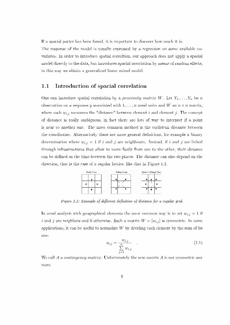
direction, that is the case of a regular lattice, like that in Figure 1.1.

Figure 1.1: Example of dierent denition of distance for a regular grid.

In areal analysis with geographical elements the most common way is to set wi,j = 1 if

i and j are neighbors and 0 otherwise. Such a matrix W = [wi,j ] is symmetric. In some

applications, it can be useful to normalize W by dividing each element by the sum of its

row:

ai,j =wi,jn∑j=1

wi,j

. (1.1)

We call A a contingency matrix. Unfortunately the new matrix A is not symmetric any

more.

6

In this work we have decided to measure the distance by a contingency matrix A as

dened in Equation (1.1).

1.2 Measures of spatial association

Before applying the model, in order to explore the presence of an eective spacial as-

sociation, it is recommended to perform some statistical tests. All test statistics that

measure the spatial autocorrelation have a common root given by the following matrix

cross-product

Γ =∑i,j

wi,jci,j (1.2)

whereW = [wi,j ] is a proximity matrix 0,1 and C represents a measure of the association

between two elements. The general cross-product Γ is a statistic in the sense that the

implied matrix is a sample of a number of possible matrices. The value of the cross-

product can be compared to the range of values that might be produced if a number of

maps with the same set of values were created by a complete random assignment of values

to locations. There are n! dierent possible maps that could be produced randomly if

each of the original values were randomly assigned. Once Γ has been calculated, if we

compute all the cross-product related to the n! possible matrices, we have generated

an empirical distribution for Γ. In this way we can estabilish if Γ is an outlier and so

decide if there is spacial correlation among areal units. This procedure is computationally

unfeasible, expecially if n is really big. It turns out to be more convenient to compute

some indices like the Moran's I or Geary's C, that derive from the cross-product but can

be asympotically approximated. In our Bayesian application we will use such indices

only for an exploratory analysis; we do not interpret them as a frequentist test of spatial

signicance.

If we set ci,j = (Yi − Y )2(Yj − Y )2 in Equation (1.2), we obtain the Moran′s Index:

I =

nn∑j=1

n∑i=1

ai,j(Yi − Y )(Yj − Y )

∑i 6=j

ai,jn∑i=1

(Yi − Y )2

.

7

Moran demostrated that if Y1, . . . , Yn are independent and equally distributed, then I is

asymptoticaly normally distributed with the following law

I ∼ N(− 1

n− 1,n2(n− 1)S1 − n(n− 1)S2 − 2S2

0

(n+ 1)(n− 1)2S20

)

where S0 =n∑i 6=j

ai,j , S1 = 12

n∑i 6=j

(ai,j + aj,i)2 and S2 =

n∑k=1

(n∑j=1

ak,j +n∑i=1

ai,k)2.

Index I belongs to [−1, 1] and we can interpretate its value as follows:

I =

I < − 1

n−1 there is evidence for negative spatial association

I = − 1n−1 there is no evidence for spatial association

I > − 1n−1 there is evidence for positive spatial association .

The expression of Geary′s C takes form

C =

(n− 1)n∑j=1

n∑i=1

ai,j(Yi − Yj)2

2∑i 6=j

ai,jn∑i=1

(Yi − Y )2

.

If Y1, . . . , Yn are independent and identically distributed then C is asymptotically normal

distributed with law

C ∼ N(

1,(2S1 + S2)(n− 1)− 4S2

0

2(n+ 1)S20

)where the above notation still holds. Usually 0 < C < 2, only in rare cases C > 2. The

interpretation is the following:

C =

0 < C < 1 there is evidence for positive spatial association

C = 1 there is no evidence for spatial association

C > 1 there is evidence fot negative spatial association .

Moran's I is a more global measurement and sensitive to extreme values of y, whereas

Geary's C is more sensitive to dierences in small neighborhoods.

8

1.3 Calculation of the joint distribution

Given our data Y1, . . . , Yn, we need to calculate the joint distrtibution p(y1, . . . , yn).

Bayesian methodology has existed for a long time, but only recently it approaches to es-

timation of these models, making them practically feasible. The computation approach

known as Markov Chain Monte Carlo (MCMC) decomposes complicated estimation prob-

lems into simpler problems that rely on the lower-dimensional conditional distributions

for each parameter in the model (Gelfand and Smith, 1990).

1.3.1 Bayesian method

In this subsection we shortly describe the basic ideas of the Bayesian analysis.

The most important aspect of the Bayesian methodology is the focus on distributions

for the data as well as for the parameters. Let X = (X1, X2, . . . , Xn) be independent

and identically distributed observations from a probability distribution f , conditionally

to some unknown parameters θ. The basic dierence between a Bayesian and frequentist

approach is that in Bayesian perspective the parameters θ are not constant, but they are

random variables. We set a prior distribution π(θ) for θ; that represents the knowledge

that we have on the topic before the analysis. If our knowledge from the prior experience

is very poor, then this distribution should represent a vague probabilistic statement,

whereas a great deal of previous experience would lead to a very narrow distribution

centered on some hyperparameters gained from previous experience. Datasets are usually

large and prior information will tend to play a minor role in determining the character

of the posterior distribution. Formally a Bayesian model is given by:

X1, . . . , Xn|θiid∼ f(x,θ) (1.3)

θ ∼ π(θ) . (1.4)

Basically, the Bayesian inference relies on the Bayes' formula

P (Ai|E) =P (E|Ai)P (Ai)

P (E)=

P (E|Ai)P (Ai)n∑k=1

P (E|Ak)P (Ak)

where A1, A2 . . . , An is a nite or innite partition of the sample space (Ω,B) such that

P (Aj) > 0 ∀j and P (E) > 0 ∀E ∈ Ω.

9

Given Equations (1.3) and (1.4), the aim is to calculate "a" posterior distribution π(θ|X)

for the parameters θ given data X, this represents an update of π(θ) after conditioning

on the sample data, i.e. the Bayes formula for density provides the posterior density

π(θ|X) =f(X|θ)π(θ)

f(X).

Since the marginal distribution of the data f(X) is independent from the parameters θ,

we can calculate the posterior density to less than a costant

π(θ|X) ∝ f(X|θ)π(θ) .

The posterior distribution forms the basis for all inference, since it contains all relevant

information regarding the estimation problem. Relevant information includes both sam-

ple data information coming from the likelihood f(X|θ), as well as past or subjective

information embodied in the prior distributions of the parameters. The prior choice is

determinant for the calculation. To semplify the procedure it is common to choose a

prior conjugate to the model, this means that the posterior distribution belongs to the

same family of the priors, but with updated parameters.

Tipically we are interested in the expected value of a function h(θ) of the parameters

Eπ[h(θ)|X] =

∫Θh(θ)π(dθ|X) .

The integral could be dicult to compute, thus we approximate the result. Rather than

working with the exact posterior density of the parameters, we simulate a large random

sample from the posterior distribution. Under some hypothesis of regularity (Harris-

recurrence and irreducibility), the invariant distribution of a Markov Chain θ1, . . . , θM is

given by the target distribution π(θ|X) when M goes to innity. Applying the strong

law of large numbers, choosen M large enough, we can approximate the mean with the

ergodic mean of the chain θ1, . . . , θM :

Eπ[h(θ)|X] =1

M

M∑i=1

h(θi) .

From a computational point of view, the only problem is to generate a sample from

the posterior when it is not in a closed form. Gibbs Sampler and Metropolis-Hastings

algorithms will be useful for this purpose. For more details about Markov Chains, see

for example Jackman (2009).

10

1.3.2 Existence and uniqueness of the joint distribution

In the context or areal data it is natural to calculate the joint distribution using the full

conditional distributions p(yi|yj , i 6= j) for i = 1, . . . , n, which usually have a simpler

formula and direct interpretation. Given p(y1, . . . , yn), the full conditional distributions

are uniquely determined, but unfortunately the converse is not always true. In addition,

using the full conditional distributions to determine a joint distribution could lead to an

improper result, even if p(yi|yj , i 6= j)'s are proper for all i. To alleviate this problem we

can apply the Brook's Lemma, that concerns the uniqueness of the joint distribution.

Brook's Lemma. Let π(x) be a density for x ∈ Rn and dene

Ω = x ∈ Rn : π(x) > 0. Then for x, x′ ∈ Ω the following holds

π(x)

π(x′)=

n∏i=1

π(xi|x1, . . . , xi−1, x′i+1, . . . , x

′n)

π(x′i|x1, . . . , xi−1, x′i+1, . . . , x′n)

=

n∏i=1

π(xi|x′1, . . . , x′i−1, xi+1, . . . , xn)

π(x′i|x′1, . . . , x′i−1, xi+1, . . . , xn).

Fixed a point y(0) = (y(0)1 , . . . , y

(0)n ), applying iteratively the Brook's Lemma, we

obtain :

p(y1, . . . , yn) =p(y1|y2, . . . , yn)

p(y(0)1 |y2, . . . , yn)

· p(y2|y(0)1 , y3, . . . , yn)

p(y(0)2 |y

(0)1 , y3, . . . , yn)

· . . .

· · · ·p(yn|y(0)

1 , . . . , y(0)n−1)

p(y(0)n |y(0)

1 , . . . , y(0)n−1)

· p(y(0)1 , . . . , y(0)

n )

for all point y = (y1, . . . , yn).

Thanks to this relation, instead of calculating the joint distribution, we can work with n

unidimensional full conditional distributions. It is worth to notice that this is very useful

for large n.

In a spacial models, referring to the proximity matrix W , we can imagine that the full

conditional distribution only depends on the set of neighbours of i, namely %i. The full

conditional distribution becomes

p(yi|yj , j 6= i) = p(yi|yj , j ∈ %i) (1.5)

We want to be sure that using local specications does not change the uniqueness and

the stationarity of the joint distribution, this assumption is largely used in the theory of

11

Markov Random Field (MRF).

Intuitively we can represent a set of random variables with a graph: every node is asso-

ciated with one variable and two nodes are connected only if the corresponding variables

are correlated. For example, the graph in Figure 1.2 rapresents a problem where there

Figure 1.2: Example of a graph.

are seven variables X1, .., X7, such that X1 and X3 are uncorrelated, while X4 and X7

are correlated.

To better understand the developement of this dissertation, we have to mention some

preliminary results on MRF.

Denition of Markov Random Field. Given an undirected graph G = (V,E), where

V is the set of nodes and E of arches, and a set of random variables Xv, v ∈ V , then

X = Xv, v ∈ V forms a Markov Random Field with respect to G if X = Xv, v ∈ V

satisfy the local Markov properties:

pairwise Markov property: if u and v are no adjacent variables, in other words

(u, v) /∈ E, then u and v are conditionally independent with respect to the other

variables, i.e.

Xu ⊥ Xv | XV \u,v ∀(u, v) /∈ E

local Markov property: a variable is conditionally independent from all other vari-

ables with respect to its neighbors, i.e.

Xv ⊥ XV \%v | X%v ∀v ∈ V

global Markov property: given A,B ∈ V and a separate subset S ∈ V such that

12

every path from node A to node B passes across S, then:

XA ⊥ XB | XS .

In order to understand the above denition, an example is a stochastic process X =

(Xt)t>0 adapted with respect to the probability space (Ω,F ,Fs, P ) 1 . In this case

the only neighbour of the variable Xt is Xt−1. A stochastic process is Markov if the

three properties above hold, in other word X is a MRF if the conditional probability

distribution of a future state depends only on the present state, i.e.

P (Xt | Xt−1, . . . , X1) = P (Xt | Xt−1) ∀t.

Since it can be dicult to verify all these properties for a generic graph, we focus on

those graphs that can be factorized by cliques. The same procedure can be extended to

all the graphs under other hypoteses.

Denition of Cliques. Given an undirected graph G = (V,E), a subset C ∈ E is a

clique if (u, v) ∈ E ∀u, v ∈ E; k = |C| is said size of the clique.

Figure 1.3: Example of clique: the subset 0, 1, 3, 4 is a clique because all the nodes are connected.

If k = 1, i.e. none node has neighbours, then the model is independent; with k ≥ 2

we start to introduce a spatial structure.

Denition of Potential function. f(x1, x2, . . . , xk) is a potential function of order k

if it is exchangeable with respect to its arguments, i.e.

f(x1, x2, . . . , xk) = f(s(x1, x2, . . . , xk))

for any s(x1, x2, . . . , xk) permutation of x1, x2, . . . , xk.1F is the σ − algebra that makes the whole the process measurable, Fs is the ltration, i.e. Fs =

σXu, ∀u < s is the σ − algebra that makes the process measurable since istant s .

13

Denition of Gibbs distribution. p(y1, . . . , yn) is a Gibbs distribution if it is a func-

tion of yi only through potential function on clique:

p(y1, . . . , yn) ∝ exp

γ∑k

∑α∈M

φ(k)(yα1 , . . . , yαk)

(1.6)

where φ(k) is a potential of order k, M is the collection of all the cliques of size k from

1, . . . , n and γ > 0 is a parameter.

In order to prove that the full conditional distributions in (1.5) dene a unique joint

distribution, one can use the following fundamental theorem of random elds.

Hammersley-Cliord Theorem. A probability distribution P with positive and contin-

uous density f satises the pairwise Markov property with respect to an undirected graph

G if and only if it factorizes according to the cliques of G.

Applying the Hammersley-Cliord Theorem, we can deduce that (1.6) is a probability

distribution on a MRF.

Now x k = 2 and take the potential function as φ = (yi − yj)2 , j ∈ %i, the Gibbs

distribution becomes

p(y1, . . . , yn) ∝ exp

− 1

2τ2

∑i,j

(yi − yj)21(i ∼ j)

(1.7)

and the respective full conditional distributions are

p(yi|yj , j 6= i) = N

∑j∈%i

yini,τ2

ni

∀i (1.8)

where ni =n∑k=1

wi,k is the number of the neighbors of unit i.

The relationship between (1.7) and (1.8) can be easily proved (see for example Carlin

and Banerjee, 2003b). From Equation (1.7), let us write the joint distribution as

p(y1, . . . , yn) ∝ exp

− 1

2τ2

∑i,j

(yi − yj)21(i ∼ j)

=n∏j=1

exp

− 1

2τ2

∑i 6=j

wi,j(yi − yj)2

=

= exp

− 1

2τ2

n∑i=1

niy2i +

n∑i=1

∑j 6=i

wi,jyiyj

.

14

Hence, collecting only the terms involving yi and keeping in mind that W is symmetric,

one nds out that

p(yi|yj , j 6= i) ∝ exp

−1

2

niy2i − 2yi

∑j 6=i

wi,jyj

.

The result in (1.8) now follows simply completing the square.

Distributions (1.8) are clearly in the form of distributions (1.5), so we have demostrated

that, given the local full conditional distributions, we can nd a unique joint distribution

for Y1, . . . , Yn.

1.4 Conditionally Autoregressive Models (CAR)

An intuitively way to dene an areal model is setting the full conditional distributions.

Dierent sets of full distributions identify dierent models. The Conditionally Autore-

gressive Model (CAR) is one of the most important; it was introduced by Besag in the

1970s and became very popular because of the simple form of its full conditional distri-

butions. See Getis (2008).

In the following we deal with normal CAR model, but CAR can be generalized to the

exponential family.

Given Y1, . . . , Yn areal data with contingency matrix A, let Y−i = (yj , j 6= i) and set

Yi|Y−i = y−i ∼ N

∑j

ai,jyj , τ2i

i = 1, . . . , n (1.9)

We can easily recognise a distribution of the form (1.7), so applying the previous results

we can obtain the joint distribution

p(yi, . . . , yn) ∝ exp−1

2y′D−1(I −A)y

where D is a diagonal matrix with Di,i = τ2

i . It seems to be a multivariate normal

distribution

Y ∼ N (0, (I −A)−1D) . (1.10)

Actually we have to verify that

Σ = (I −A)−1D

15

really represents a covariance matrix. If we set τ2i = τ2/ni, it is immediate to verify the

simmetry of

Σ−1 = D−1(I −A) = (Dw −W )/τ2

where Dw is diagonal with (Dw)i,i = ni. Instead (Dw−W )1 = 0, so Σ−1 is singular.

Hence the joint distribution of Y is improper. This is a problem if we want to use (1.6) as

a model for data. One way to avoid this problem is to weight the mean of the neighbours

by a suitable parameter ρ 6= 1, in such a way that Σ−1 becomes Σ−1 = Dw − ρW . The

full conditionals become

Yi|Y−i = y−i ∼ N

ρ∑j

ai,jyj ,τ2

ni

i = 1, . . . , n (1.11)

The model described in (1.10) is named proper CAR . We have to choose a value of

ρ that makes Σ−1 non singular. There are dierent approches that lead to dierent

intervals of values. The rst one is based on the

Gershgoring disk Theorem. Given a symmetric matrix C, if ci,i > 0 and∑i 6=j|ci,i| < ci,i

for all i, then C is positive denite.

We can apply this result to Dw − ρW that is symmetric and a sucient condition

that implies Gershgoring Theorem is |ρ|< 1.

The second one provides a more narrow interval: in literature it has been proved that

Dw − ρA is non singular if 1λ1< ρ < 1

λn, where λ1 < λ2 < · · · < λn are the eigenvalues

of D− 1

2w WD

− 12

w . In a Bayesian context, a classical prior distribution for ρ is a uniform

distribution in the selected interval, i.e.

ρ ∼ U(

1

λ1,

1

λn

).

Parameter ρ can be interpretated as a measure of the spatial correlation between the

data. One can prove that λn is equal to 1 and that λ1 < 0. There is a strong positive

spatial correlation for 0.8 < ρ < 1, instead if there is negative correlation, then ρ would be

negative. We notice that ρ could be 0, this is equivalent to set up an independent model,

without spatial correlation. It is important to underline that, despite the introduction of

the variable ρ is necessary to obtain a proper joint distribution, it changes the mean of

16

the conditional disribution (see 1.10) and can reduce the breadth of the spatial pattern.

Referring to (1.10), we may re-write the system of random variables as

Y = ρWY + ε

Y = (I − ρA)−1ε .

A fundamental feature of this model is that the vector of errors has the law

ε ∼ N (0, D(I −A)′) .

In other words the errors are not independent as in a general linear regression, this is

because we are modeling spatial dependence.

It is possible to introduce a regression component into (1.10), without changing the idea

of the model, but only adding a term in the mean structure as follows:

Y |X,β, τ2, ρ ∼ N (Xβ, (I − ρA)−1D) . (1.12)

Finally note that by means of (1.7) an equivalent rapresentation of (1.11) in terms of full

conditionals is provided by

Yi|X,Y−i,β, τ2, ρ ∼ N(X ′iβ + ρAiY ,

τ2

ni

)i = 1, . . . , n . (1.13)

1.4.1 Introduction of spatial random eects

As we previously said, we do not apply a CAR model to the data, but we prefer to

introduce some spatial random eects. A model alternative to (1.12) can be obtained by

substituting ρAiY in the mean structure with one spatial random eect φi for each i,

such that Φ = (φ1, . . . , φn) evolves as a spatial CAR model. We introduce the notation

Φ ∼ CAR(A, τ2, ρ) (1.14)

that stands for

Φ ∼ N (0, (I − ρA)−1D) .

Furthermore Y1, . . . , Yn are assumed to be independent with

Yi|β, τ2, ρ ∼ N (Xiβ + φ, ci) (1.15)

17

where ci is a generic notation for the variance of yi. It is worth to underline that if we

expect areal correlation among Y1, . . . , Yn and we set a linear regression model

Y ∼ N (Xβ,Σ)

the covariance matrix Σ is not diagonal and hence Y1, . . . , Yn are not independent. This

represents a problem in a statistical analysis because we need to factorize the likelihood

expression: for this reason it is recommended to set the model in the form (1.13) and

(1.14).

We can nd lots of exemples of this approach in literature; one can see frameworks

like Stern and Cressie (1999), Banerjee and Carlin (2015), Epifani and Nicolini (2015b)

among the others.

18

Chapter 2

Time series

A time series process Xt, t ∈ T ia a stochastic process or a collection of random vari-

ables Xt indexed in time. If T ⊆ N then the process is discrete in time, if T ⊆ R then it

is a continuous time random process. We will indicate with Xt, t = 1, . . . , T , a collection

of T equally spaced realization of a time series process.

The aim of time series analysis is to describe the dependence among a sequence of ran-

dom variables, the hypotesis is that they can not be independent realizations from a

unique distribution. If we are able to identify a trend, i.e. a stochastic process that has

trajectories that describe the data, it is possible to make prevision for the value in the

future.

Many time series models are based on the assumption of stationarity.

Dedinition of strong stationarity. A time series process Xt, t ∈ T is strongly

stationary if, for any sequence of time t1, . . . , tn and any lag h, the probability distribu-

tion of the vector (Xt1 , . . . , Xtn) is identical to the probability distribution of the vector

(Xt1+h, . . . , Xtn+h).

This mean that the realizations of the process do not depend on the starting time.

However this denition is not operative, because it is dicult to verify for a generic

process. We can apply the denition of weak stationarity.

Denition of weak stationarity. A time series process Xt, t ∈ T is weakly stationary

if, for any sequence of time t1, . . . , tn and any lag h, the rst and the second moments of

19

the vector (xt1 , . . . , xtn) are identical to the rst and the second moments of the vector

(xt1+h, . . . , xtn+h).

In other words, the mean and the variance of the process are constant over time, and

the covariance function γ between two dierent realizations depends only on del lag of

the time, i.e.

E[Xt] =µ ∀t ∈ T

V ar[Xt] =v ∀t ∈ T

Cov(Xt, ys) =γ(t− s) ∀s < t ∈ T .

Intuitively, a stochastic process is stationary if its probabilistic structure is constant

over time, so that the process is easyer to analyse.

In an arbitrary model we can set Xt as a function of the past values, of some parameters

θ and of the estimation error ε, i.e.

xt = f(x0, x1, . . . , xt−1,θ, ε) ∀t.

From a Bayesian point of view, once set a prior distribution on the parameters π(θ), we

can apply the Bayes' Theorem, and get the posterior distribution

p(θ|x0, . . . , xt) ∝t∏

n=1

p(xt|x−t,θ)p(x0|θ)π(θ) .

In a more complex case it can happen that also the parameters depend on the time

(θt)t∈T and we have to introduce a dynamic for the behavior of the parameters

xt = f(x0, x1, . . . , xt−1,θt, ε) ∀t

θt = g(θ0, θ1, . . . , θt−1,Φ, ν) ∀t.

In this case it becomes more dicult to obtain the posterior distribution for θt because

the calculus depends on the specic case.

A useful method to verify the dependence between the data is by the autocorrelation

function (ACF) ρ dened as

ρ(xs, xt) =γ(s, t)√

γ(s, s)γ(t, t), ∀s, t ∈ T .

20

If the model is stationary and h = |t− s|, we can write the ACF function in the form

ρ(h) =γ(h)

γ(0).

If ρ(h) is dierent from zero there is an eective correlation among the data.

2.1 Autoregressive Models

Among the several dierent models for time series, let us discuss the properties of the

Autoregressive (AR) models, because they are the simplest class of empirical models for

exploring dependences over time. So they are the basis for more complex models.

In AR models the random variable Xt is function of the past values.

Denition of AR models. Xt is an Autoregressive model of order p (AR(p)) if

Xt =

p∑j=1

φjXt−j + εt t = 1, 2, . . .

where εt is the error at time t.

We assume that the errors are independent and normally distributed:

εt ∼ N (0, v) ∀t.

The sequential nature of the model implies a sequential structure of the data distribution

p(x1, . . . , xT |φ, ε) = p(x1, . . . , xp|φ, ε)T∏

t=p+1

p(xt|xt−1, . . . , xt−p,φ, εt) .

We assume to know the initial values x1, . . . , xp, so we obtain

p(x1, . . . , xT |x1, . . . , xp,φ, ε) =T∏

t=p+1

p(xt|xt−1, . . . , xt−p,φ, εt) = N (F ′φ, vI) (2.1)

where F = [fT , . . . ,fp+1] and ft = (xt−1, . . . , xt−p)′. The above distribution is very

generic, we can introduce some extensions like a nonzero mean for the variable Xt, a

variance of the error that changes over time, etc.

21

2.1.1 Stationarity for AR models

Let us now introduce some criteria in order to guarantee AR models stationarity.

Denition of causality. An AR(p) process is causal if it can be written as a linear

process dependent on all the past events

Xt =∞∑j=0

ψjεt−j .

In order to verify this condition, let us write the model using a backshift operator s,

i.e. xt−1 = sxt such that

xt = φ1xt−1 + · · ·+ φpxt−p + εt

xt − φ1xt−1 − · · · − φpxt−p = εt

xt(1− φ1s− · · · − φpsp) = εt

xt = Φ−1(u)εt

Φ(u) is called autoregressive characteristic polynomial, and xt is causal if the roots u of

Φ−1(u) = 0 satisfy |u| > 1. This causality condition implies stationarity. Alternatively,

we can write the characteristic polynomial as Φ(u) =p∑j=1

(1− αju), in this case uj = 1αj

and the causality condition becomes |αj | < 1.

2.1.2 Autocorrelation structure and Partial Autocorrelation Function

The autocorrelation structure of an AR(p) is given in terms of the solution of the equation

ρ(h)− φ1ρ(h− 1)− · · · − φpρ(h− p) = 0 h ≥ p (2.2)

Let us call m1 . . . ,mr the multiplicy of the roots of Φ(u). Then the general solution of

(2.2) is

ρ(h) = αh1p1(h) + αh2p2(h) + · · ·+ αhrpr(h) h ≥ p

where pj(h) is a polynomial of degree mj − 1.

Another important quantity to better understand the correlation between the data is

the Partial Autocorrelation Function (PACF). The PACF is a function dened by the

coecients at lag h, each coecient φ(h, h) is a function of the best linear predictor of

22

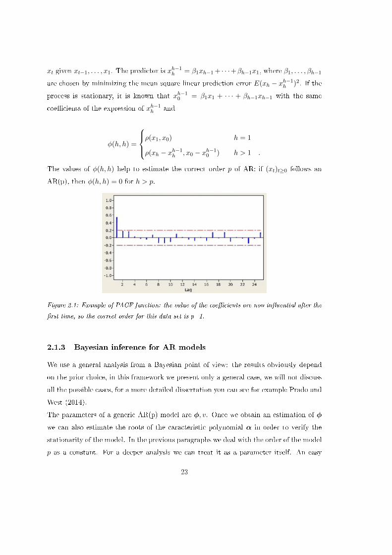
xt given xt−1, . . . , x1. The predictor is xh−1h = β1xh−1 + · · ·+βh−1x1, where β1, . . . , βh−1

are chosen by minimizing the mean square linear prediction error E(xh − xh−1h )2. If the

process is stationary, it is known that xh−10 = β1x1 + · · · + βh−1xh−1 with the same

coecients of the expression of xh−1h and

φ(h, h) =

ρ(x1, x0) h = 1

ρ(xh − xh−1h , x0 − xh−1

0 ) h > 1 .

The values of φ(h, h) help to estimate the correct order p of AR: if (xt)t≥0 follows an

AR(p), then φ(h, h) = 0 for h > p.

Figure 2.1: Example of PACF function: the value of the coecients are non inuential after the

rst time, so the correct order for this data set is p=1.

2.1.3 Bayesian inference for AR models

We use a general analysis from a Bayesian point of view: the results obviously depend

on the prior choice, in this framework we present only a general case, we will not discuss

all the possible cases, for a more detailed dissertation you can see for example Prado and

West (2014).

The parameters of a generic AR(p) model are φ, v. Once we obtain an estimation of φ

we can also estimate the roots of the caracteristic polynomial α in order to verify the

stationarity of the model. In the previous paragraphs we deal with the order of the model

p as a constant. For a deeper analysis we can treat it as a parameter itself. An easy

23

way to determine the correct value of p is to repeat the analysis with an increasing value

of it and compare the results according to some criterion like AIC or BIC for example.

The only precaution is to use a value of p small enough with respect to T, otherwise

problems like overtting or collinearity can occur. In a Bayesian context we assume a

prior distribution over p.

The posterior distribution is

π(φ, v, p|x) = p(xT , . . . , xp+1|φ, v, p, xp, . . . , x1)π(xp, . . . , x1|φ, v, p)π(φ, v|p)p(p)

In this section we do not really care about the prior distribution on p, we limit our con-

sideration on the prior distributions π(φ, v|p) and statistical model p(xp, . . . , x1|φ, v, p)

and consider p as a xed number.

There are two dierent ways to select a prior for the initial values: the rst one is to

choose a distribution independent from the parameters, just to initialize the time se-

ries, in this case the analysis is independent by the initial values. The second way is to

set a prior distribution that depends on the parameters; under this hypothesis the nal

result could dependent on the initial values: the eect of the initial values is xed, if

the time serie is "long", i.e. T p, then p(xp, . . . , x1|φ, v, p) is negligible with respect

to p(xT , . . . , xp+1|φ, v, p, xp, . . . , x1), otherwise the analysis will depend on the value of

x1, . . . , xp.

The choice for π(φ, v|p) is more relevant. First of all it is important to remind that the

prior for φ and v should be concentrated only in the stationarity region and be zero

outside. In a simulation approach there is no way to verify stationarity condition before

having estimated α, so as we have said previously, rstly we have to estimate φ, then

calculate α. The simplest method is to proceed in an unconstrained analysis and then

reject the values of φ that stay outside the stationarity region. If the model is really

stationary, the rejection rate will be low and the analysis reliable. But it can happen

that the rejection rate is high; in such a case probably the stationarity assumption does

not work for the model, the analysis is not ecient and hence other methods are needed.

The prior π(φ, v|p) depends strongly on p, to avoid problems in calculation it is suggest

to assume an improper prior

π(φ, v|p) ∝ 1

v.

24

Under stationarity assumption, the problem has a multinormal likelihood

p(xp, . . . , x1|φ, v, p) ∼ N (0, vAφ)

p(xT , . . . , xp+1|φ, v, p, xp, . . . , x1) ∼ N (F ′φ, vI)

so we obtain

p(xT , . . . , x1|φ, v, p) ∝1

vT/2|Aφ|1/2×

× exp

(xT , . . . , xp+1)′(F ′φ)−1(xT , . . . , xp+1) + (x1, . . . , xp)

′A−1φ (x1, . . . , xp)

2v

In order to obtain a conjugate model, the best prior choice for the parameters is the

Jereys' prior π(θ) ∝√|I(θ|x)|, where I(θ|x)i,j = −E[∂2log(p(x|θ))/∂θi∂θj ]. In liter-

ature (see Box, Jenkins and Reinsel, 2008) it is known that Jereys' prior for this specic

problem is approximately π(φ, v) ∝ |Aφ|1/2v−1/2. With this prior we can proceed with a

Gibbs algorithm, because the full conditionals are known "popular" distribution: inverse-

gamma for v and multinormal distribution for φ.

25

26

Chapter 3

A model for the population density

In this chapter, we introduce the data set and the general goal of the analysis, then we

compare dierent models in order to interpret the problem. After describing the model,

the calculation of the full conditionals and the sampling scheme are illustrated.

3.1 The data

The analysis is applied to the state of Massachusetts. The data set comes from the

NHGIS project1; it contains the census tract data for the period between 1970 and

2010. As the census are repeated every 10 years, then the data are aected by the

important changes in the census tract composition across time, anyway it is possible

to compare them over dierent periods thanks to the fundamental re-elaboration made

by the NHIGIS project, that grants compatibility across time. The most dierence is

between the rst and second time (1970 and 1980 ) with the other periods ( 1990-2010

). During the analysis it becomes clear that the result obtained in 1990-2010 are more

accurate.

First of all it is important to explain what a census tract is: according to the denition

provided by the US census, a census tract is dened as a spatial area whose population

size ranges between 1500 and 8000 inhabitants, with an optimal size of 4000.

Massachusetts has 14 counties.

1Minnesota Population Center. National Historical Geographic Information System: Version 2.0.

Minneapolis, MN: University of Minnesota 2011.

27

Figure 3.1: Massachussettes state.

Each county is divided in census tracts, each of them has a centre in which the in-

formation about the population are collected. The peculiarity of the data set is that

the whole number of census tract changes every year: when a census tract becomes too

populated, then it is splitted, while in the opposite case it is absorbed by another one.

This means that the census tract evolution is not easily traceable over time, even if they

are all identied by a sequential string code: so we cannot describe the evolution of a

single census tract over time. But we can study the dynamic of the distribution of the

population density across each county. Our observations are the census tracts density y

computed as the total population divided by the area of the census tract.

As we mentioned above, the goal of the analysis is to determine which "global"

features lead the individual choice, in addition to the personal preferences. The most

relevant variable is the distance between Boston and each census tract, calculated as the

euclidean distance between the geographic coordinates of Boston and the centroid of the

census tract. Previous study (see Epifani and Nicolini, 2013) states that the distance

from Boston is the key element for modelling population distribution. In order to focus

the contest, we have to introduce the concept of Central Business District (CBD): it

is a selected point which includes services, leisure activities, professional and economics

28

centres, infrastructure elements that guarantee mobility.

Once a CBD has been identied, it turns out to be the centre of the density population

distribution (see Helsey and Strange, 2007). Economic literature selected Boston as the

most attractive city in Massachusetts (see Glaeser, 2005) and it maintained its attractiv-

ness across time, since the census tract with highest density have always been in Boston's

county. It is important to remind that distance can not be considered costant over time

because the census tract changes every time.

Despite the distance from Boston is determinant, basing the analysis only on this pre-

dictor would be too restrictive, in fact there are other factors that can have a relevant

role, like for example natural amenities and etnic composition (see Topa and Zenou,

2015). The presence of natural amenities can have an important role in the decision

process, because they contribute to create space for leasure time. The water is taken as

a prototype of amenities because it is the most attractive natural element. Hence it is

available a variable zeta that summarizes the proportion of water's area in the county;

Epifani and Nicolini (2015) has argued that zeta can be considered constant over time.

We should also focus on further variables that allow to describe "the reputation" of a

zone, these variables are the ethnic composition, the income and the education level. It

is easy to understand that an individual prefers to settle close to individuals who share

the same level of income and education, but especially who belong to the same ethnic

group. As an indicator of the ethnic composition we take the proportion mix of white

individuals over the total population. As for the income we introduce two distinct local

predictors: an indicator of the level of the income per-capita (income) per-census tract,

and a measure of the dispersion and inequality of income measured by the Gini index

(gini). The variable income is not collected in 1970, so we do not use it in the regression

for the rst period. The census provides us the joint data on the income's distribution,

there are 4 classes for each census tract: income less than 10000 dollars, income between

10000 and 15000 dollars, income between 15000 and 25000 dollars, and nally income

more than 25000 dollars. We compute the frequencies on the classes and from that the

Gini index with the formula

gini =

∑n−1i=1 (Pi −Qi)∑n−1

i=1 Pi

29

where Qi are the cumulative percentage of the income and Pi are the cumulative per-

centage if the income would be equidistributed. The Gini index varies between 0 and

1; its value is equal to 0 when there are no inequalities, and increases with inequality,

to reach 1 when one individual earns the entire income of the census tract. Instead, in

order to propose a comprehensive indicator of the distribution of the education in each

census tract we elaborate a synthetic measure of the degree of education (education)

by ranking all of the census-tracts according to the level of education of its population.

First, we rank them according to the relative frequency of citizens having a high degree of

education, and then according to the relative frequency of persons having a low degree of

education. Hence, for each census tract unit we subtract the second value of ranking from

the rst. This type of index presents the extent to which a census tract unit may emerge

as a highly educated in respect to the rest of the census tract units in Massachusetts.

Let us now summarize all the covariates; for each time t = 1, . . . , 5, for each census tract

j = 1, . . . , J [t] and for each county i = 1, . . . , 14 we have the following information:

dist(t)j : euclidean distance of census tract j from Boston;

mix(t)j : proportion of white individuals;

education(t)j : education level;

gini(t)j : Gini index;

income(t)j : income pre-capita;

cc(t)j : county of the j-th census tract;

zi : amenities in county i;

y(t)j : population density of j-th census tract.

30

3.2 Descriptive statistic

In this section we present an exploratory analysis of the data set.

First of all, let us standardize the predictors substracting the mean and dividing by the

standard deviation for year. Furthermore, we transform the population density to a log-

function Y(t)j = log(Y

(t)j ) ∀j,∀t.

We can assert that there are no drammatical change in the population during the whole

period, Figure 3.3 rapresents the mean of the logarithm of the population's density for

every county and we can see that it is almost constant. We can deduce that the analysis

is photographing the evolution of a population's density in normal conditions.

Figure 3.2: Evolution of the mean of ppopulation log-density for every county during the year

1970 (t=1), 1980 (t=2), 1990 (t=3), 2000 (t=4), 2010 (t=5). Notice that data in Barnstable,

Franklin, Dukes, Nantucket are not collected in 1970 and 1980 (see Table 3.1) .

It is worth to do some consideration on the census tracts. Referring to Figure 3.4

and Table 3.2, it is clear that the most the population lives in Suolk, where there is the

CBD of Boston, and in the nearby counties. In Suolk there are lots of census tracts,

they are really small so we expected that the population density is very high (as one can

see in Table 3.4). In faraway counties, like for example Franklin or Barnstable, there

is a little number of census tracts, they are more extended and have a lower density.

31

The mean of population density is shown in Table 3.3. It is quite clear that we expect

that the distance from Boston would be relevant in the descriprion of the evolution of

population distribution, there is a strong negative correlation between the two variables

( see the scatterplot in Figure 3.6 ).

1970 1980 1990 2000 2010

Barnstable 0 0 50 50 56

Hampshire 27 25 30 31 35

Berkshire 15 32 34 41 39

Middlesex 249 271 277 297 317

Bristol 102 105 106 116 125

Nantucket 0 0 4 5 5

Dukes 0 0 4 4 4

Norfolk 101 103 117 121 130

Essex 112 136 146 156 162

Plymouth 46 84 90 90 99

Franklin 0 0 15 16 18

Suolk 168 177 183 175 193

Hampden 71 83 87 92 103

Worcester 158 157 159 163 171

Table 3.1: Number of census tracts for each county per year .

Regarding the other covariates, we observe a negative correlation between density

population and mix of the population and a positive one between population's density

and Gini index. So we expect that people prefer to move to more comfortable place with

economic wellness and a high percentage of white people.

32

1970 1980 1990 2000 2010

Barnstable NA NA -1.60 -1.43 -1.47

Hampshire -1.59 -1.44 -1.31 0.-1.28 -1.43

Berkshire -0.81 -1.76 -1.86 -2.20 -2.27

Middlesex 0.58 0.40 0.39 0.39 0.41

Bristol 0.05 0.007 0.009 0.01 -0.02

Nantucket NA NA -2.18 -2.52 -2.55

Dukes NA NA -2.77 -2.52 -2.40

Norfolk -0.07 -0.09 -0.04 -0.001 0.02

Essex 0.43 0.17 0.19 0.19 0.19

Plymouth -0.71 - 0.87 - 0.82 -0.75 -0.75

Franklin NA NA -2.49 -2.38 -2.45

Suolk 1.84 1.71 1.73 1.79 1.92

Hampden -0.05 -0.09 -0.06 -0.10 -0.14

Worcester -0.80 -0.87 -0.76 -0.72 -0.69

Table 3.2: Population's log-density mean for each county per year .

1970 1980 1990 2000 2010

Distance 0.067 -0.288 -0.486 -0.520 -0.537

Mix -0.281 -0.391 -0.509 -0.588 -0.632

Gini -0.185 0.531 0.489 0.483 0.505

Education 0.066 -0.300 -0.316 -0.345 -0.322

Amenities 0.406 0.400 0.319 0.327 0.350

Table 3.3: Correlation between the covariates and log-density per year.

By the preliminary analysis we nd out that for the rst two years we do not have

data for four counties, i.e. Barnstable, Nantucket, Dukes and Franklin, because in 1970

and 1980 there were not a structure of city and population distribution that allow to

dene a census tract. Anyway this do not aect the analysis.

Since the goal of this work is looking for a geographical dependence among data, we

33

Figure 3.3: Distribution of population density per year: in general the density is quite small over

time.

Figure 3.4: Graph of population's log-density and distance per year.

delete those census tracts that have no neighbours or whose population's density is equal

to zero. We interpret this occurrence as an error in the collection of data. We end up

with a data set composed by a dierent number of census tract J [t] for every year. As it

34

is reported in Table 3.4, the total number of census tracts grow up over time, so there is

an increment of population. Comparing Figure 3.5 and Figure 3.6, we can clearly see

1970 1980 1990 2000 2010

J 1049 1173 1302 1357 1457

Table 3.4: Total number of census tracts in Massachusetts for every year.

the evolution of the census tracts. In 1970 the population density is low, the most part

of the population settles near to the biggest cities while in the countryside there are even

spaces without census tracts, i.e. the withe space in the map; in such place we do not

have informaion. In 50 years the population has grown: the mean of the density is almost

constant, but the number of census tacts has increased, especially near to the cities and

in Suolk (see Table 3.1 and 3.2). Even if the cities remain the residencial centre because

of services, aniway the population is spread all over the state, in fact there is not lack of

census tracts any more, this means that there are people and structures enough to dene

a census tract.

35

Figure 3.5: Map of census tracts in Massachusettes in 1970.

36

Figure 3.6: Map of census tracts in Massachusettes in 2010.

37

In order to investigate the spatial correlation, we calculatedMoran′s I andGeary′s C

indices; their values are reported in Table 3.5.

1970 1980 1990 2000 2010

Moran′s I 0.56 0.61 0.62 0.61 0.64

Geary′s C 0.32 0.28 0.28 0.27 0.21

Table 3.5: Spatial indices.

The Moran′s I is positive and its value is in the middle between zero and one, hence

we expected a global dependence, even if it is not very strong. The local correlation

seems to be more pronunced, since the Geary′s C takes value quite close to zero. Both

indices are quite constant, both point out a little increment of the spatial correlation

over time.

3.3 The model

A Bayesian approach to the problem is usefull because, by dening a prior structure

ad hoc, it allows to model time and spatial dipendences.

In order to study the spatial correlation, we propose a comparison between three models,

that describe dierent aspects of the spatial dependence. The rst model, assumed as

baseline reference, exploits the segmentation of the data within the geographic areas,

given by the counties, to assess the population density; the regressors are: distance, mix,

education, Gini index, income and amenities z. The second model is the rst attempt to

outline behavior unexplained; it is obtained by adding independent census tracts random

eects. In the third model the random eects are accounted for in a correlated way by

means of a CAR model.

In the next the three models are presented in details.

Baseline model

First of all, we address the problem setting a baseline model without any spatial random

eects. We implement a regression using the amenities z with the following individual

covariates V(t)

1,j , V(t)

2,j , V(t)

3,j , V(t)

4,j , V(t)

5,j and an iteration term V(t)

6,j :

38

V(t)

1,j V(t)

2,j V(t)

3,j V(t)

4,j V(t)

5,j V(t)

6,j

Distance Mix Gini Educ Income Income ∗Dist

The statitical model is

log(Y(t)j )|V (t)

j , zi[j], b(t)0 , b

(t)1 ,β(t), νi[j], σ

2,Σβ ∼ N (b(t)0 + b

(t)1 zi[j] + V

(t)j β(t), σ2νi[j])

independent ∀j = 1, . . . , J [t],∀t = 1, . . . , 5 .

(3.1)

In Equation 3.1 the notation i[j] species the county i of the census tract j.

The time dipendence is caugth by the regression coecients. For b(t)0 , b

(t)1 , β

(t)1 , . . . , β

(t)6 we

assume an AR(1) structure. We suppose that the initial values b(0)0 , b

(0)1 , β

(0)1 , . . . , β

(0)6 are

independent from the hyperparameters. In this way our hypotesis is that the distribution

of the population at time t in some way depends on the distribution at time t− 1. The

evolution of the regression coecients is

B(t) = (b(t)0 , b

(t)1 , β

(t)1 , . . . , β

(t)6 )

B(0) ∼ N (0, 102I)

B(t)|B(t−1),ΣB ∼ N (B(t−1),ΣB) ∀t = 1, . . . , 5

ΣB = diagσ2b0, σ

2b1, σ

2β1 , . . . , σ

2β6

The dynamic structure of the coecients is the same in all the models that we propose.

Another hypothesis is that there is a county's eects, in other words, census tracts be-

longing to the same county have same shared features not included within the other

covariates. For this reason, we add z as a covariate in the model. We remind that z is a

variable relative to the counties and represents the amenities of the county.

We also use a particular variance structure that can accommodate heteroscedastic dis-

turbances or outliers. This particular form for the variance was introduced for linear re-

gression by Geweke (1993). A set of variance scalars (v1, v2, ..., v14) represents unknown

parameters that allow us to assume the error ε ∼ N (0, σ2V ), where V is a diagonal

matrix containing parameters (v1, v2, ..., v14). All the vi are iid and their priors take

the form of a set of independent IG (r/2, r/2) distributions. This allows us to estimate

39

the additional 14 variance scaling parameters vi by adding only a single parameter r to

our model. We decide to adopt this structure for variance: in our model the idea is to

set one variable νi for each county, so we can capture heteroschedasticy among dierent

counties by comparing the value of ν. From a pracical point of view, in literature the

hyperparameter r has been set equal to 4, for more details one can see LeSage and Pace

(2009). While the variable σ2 is constant for every census tract, σ2 wants to capture the

intrnisec variability that is common to the log density of population of all census tracts.

Therefore the variance prior is

νi ∼ IG(r

2,r

2

), ∀i = 1, . . . , 14

r = 4

σ2 ∼ IG(0.001, 0.001) .

In the baseline model (3.1), the prior distributions for the variances of the regression

parameters are choosen in a standard way to be not informative, i.e.

σb0 , σb1 , σβ1 , . . . , σβ6iid∼ U(0, 10) .

It is worth to underline that all the variances' structures are independent on the time.

This is a strong assumption because we adrm that the variability of the phenomenon is

constant over time.

Indipendent random eect model

The basic idea for the second model is to verify if, in addition to heteroschedasticy among

counties, there is heterogenity even among the census tracts. For this reason we add a

random eect φ(t)j for each census tract j. The random eects are all independent each

other; they aim at capturing outliers and census tract's behavior, that is particularly

dierent from the others. The resulting normal model is:

log(Y(t)j )|V (t)

j , zi[j], (b(t)0 +b

(t)1 ,β(t), νi, σ

2,Σβ, φ(t)j , ρ

(t), τ (t) ∼ N (φj+b(t)0 +b

(t)1 zi[j]+V

(t)j β(t), σ2νi[j])

independent ∀j = 1, . . . , J [t],∀t = 1, . . . , 5

(3.2)

40

whereas, the corresponding prior structure is:

νi ∼ IG(r

2,r

2

), ∀i = 1, . . . , 14

σ2 ∼ IG(0.001, 0.001)

B(t) = (b(t)0 , b

(t)1 β

(t)1 , . . . , β

(t)6 )

B(0) ∼ N (0, 102I)

B(t)|B(t−1),ΣB ∼ N (B(t−1),ΣB) ∀t = 1, . . . , 5

ΣB = diagσ2b0 , σ

2b1 , σ

2β1 , . . . , σ

2β6

σb0 , σb1 , σβ1 , . . . , σβ6iid∼ U(0, 10)

φ(t)j |λ

(t) ∼ N(

0, λ(t))∀j = 1, . . . , J [t], ∀t = 1, . . . , 5

λ(t) iid∼ IG(0.001, 0.001) ∀t = 1, . . . , 5

We xed the same regressors and the same structure for the regression coecients and

the variance.

Proper CAR model

The innovative contribution of this work is the study of neighbours inuence at a census

tract's level. In order to explore the spatial correlation, we introduce the contingency

matrix A(t) such that

A(t)i,j =

1

n(t)i

if the census tract i and j are closed

0 otherwise

where n(t)i is the number of neighbours of the i− th census tract at time t. We introduce

a random eect for each census tract, which evolves as a CAR model. The resulting

Bayesian proper CAR model is the following:

log(Y(t)j )|V (t)

j ,β(t), νi[j], σ2,Σβ, φ

(t)j , ρ

(t), τ (t) ∼ N (φj + b(t)0 + b

(t)1 zi[j] + V

(t)j β(t), σ2νi[j])

independent ∀j = 1, . . . , J [t],∀t = 1, . . . , 5

(3.3)

41

νi ∼ IG(r

2,r

2

), ∀i = 1, . . . , 14

σ2 ∼ IG(0.001, 0.001)

B(t) = (b(t)0 , b

(t)1 , β

(t)1 , . . . , β

(t)6 )

B(0) ∼ N (0, 102I)

B(t)|B(t−1),ΣB ∼ N (B(t−1),ΣB) ∀t = 1, . . . , 5

ΣB = diagσ2b0 , σ

2b1 , σ

2β1 , . . . , σ

2β6

φ(t)j |Φ

(t)−j , τ

(t), ρ(t) ∼ N

(ρ(t)A

(t)j Φt,

τ (t)

n(t)j

)∀t = 1, . . . , 5, ∀j = 1, . . . , J [t]

Moreover the specication for the hyperparameters is

σ2σ2b0,σ2

b1,β1, . . . , σ2

β6

iid∼ IG(0.001, 0.001)

ρ(t) iid∼ U(0, 1) ∀t = 1, . . . , 5

τ (t) iid∼ IG(0.5, 0.005) ∀t = 1, . . . , 5 .

This choice is made in order to specify vague prior distribution and to have distributions

coniugate to the model. We have uninformative and constant over time prior for all

the variances, exept for τ (t). As regard to the particolar choice of the prior of τ (t), it

is important to assess whether the prior allows for all reasonable levels of variability, in

particular small values should not be excluded. As pointed out by Kelsall and Wakeeld

(1999), a prior IG(0.001, 0.001) for the precision parameter of the spatial random eects

in a CAR model, tends to place most of the prior mass away from zero (on the scale

of the random eects standard deviation), and so in situations when the true spatial

dependence between areas is negligible (i.e. standard deviation close to zero) this may

induce artefactual spatial structure in the posterior. For this reason, following Kelsall

and Wakeleld (1999), we set an IG(0.5, 0.005) distribution for τ (t). This expresses the

prior belief that the random eects standard deviation is centred around 0.5 with a 1%

prior probability of being smaller than 0.01 or larger than 2.5 (see Manual of GeoBUGS,

2014). Since we need to calculate the eigenvalues of the matrix I − ρ(t)A(t) (see in the

Appendix A the calculus for the posterior distribution of ρ(t)), then we try to prove a

relation with the eigenvalues of the matrix A, such that we do not need to calculate them

42

in every iteration. Let λ(t)j for j = 1, . . . , J [t] denote the eigenvalues of the matrix A.

They are obtained by solving the equation

det(A(t) − λI) = 0 .

In order to compute the eigenvalues µ(t)j of the matrix I − ρ(t)A(t) we set

det(I − ρ(t)A(t) − µI) = 0

det(−ρ(t)A(t) − (µ− 1)I) = 0

(−ρ(t))J [t]

(A(t) − µ− 1

−ρ(t)I

)= 0 .

If ρ(t) is dierent from zero we can semplify and obtain the following relation between

λ(t)j and µ

(t)j :

µ(t)j = 1− ρ(t)λ

(t)j ∀j = 1, . . . , J [t] .

By the way, to avoid to sample a zero value for ρ(t), we take in the interval of the prior

distribution with respect to the one shown in the theorical dissertation. This fact does

not imply any restriction in the analysis because, from the spatial indices ( Moran's I

and Geary's C ), we expect a positive and low spatial correlation.

43

3.4 Computational strategy

In this section, we illustrate the MCMC strategy used to sample from the posterior

distribution of the parameters. We refer in the following to the proper CAR model.

3.4.1 Gibbs Sampler

The posterior distribution of the proper CAR model is

β(0),β(1), . . . ,β(5), σ2,ν,Φ(1), . . . ,Φ(5),Σβ, τ(1), . . . , τ(5), . . .

. . . ρ(1), . . . , ρ(5)|Y (1), . . . ,Y (5), V (1), . . . , V (5) ∝

∝5∏t=1

[π(Y (t)|β(t),ν, σ2,Φ(t), V (t))]π(β(1), . . . ,β(5)|β(0),Σβ)π(β(0))π(Σβ)π(σ2)π(ν)×

×5∏t=1

[π(Φ(1), . . . ,Φ(5)|ρ(t), τ (t))π(ρ(t))π(τ t)] ∝

∝5∏t=1

[π(Y (t)|β(t),ν, σ2,Φ(t), V (t))π(Φ(1), . . . ,Φ(5)|ρ(t), τ (t))π(ρ(t))π(τ t)π(β(t)|β(t−1),Σβ)]×

× π(ν)π(Σβ)π(σ2)π(β(0))π(ρ(t))π(τ (t)) .

Because of the high number of parameters, it is quite complex to use standard R

library like Stan or Jags, because they are very slow. We apply the Gibbs Sampler algo-

rithm, that allows us to sample from the posterior distribution.

The basic idea of a Gibbs Sampler is to sample not directly from the posterior distri-

bution, that usually has a complicated and unknown form, but to sample from the full

conditional distributions of the parameters and update them one by one, using at each

step the last sampled parameters. This type of algorithm results particularly ecient for

this model because, as we said before, it is the best way to approach to a CAR model.

In addition almost all the priors have a conjugated form at the full conditionals level, so,

despite the huge number of parameters, the calculation of the full conditional distribu-

tions is feasible.

We illustate a general scheme of the algorithm, then we give the details of the full con-

44

ditional distributions.

Algorithm 1 Gibbs sampler algorithm

Initialise the coecients β(0) randomly sampling from N (0, 100)

Initialise the coecients βh = 0 ∀h = 1, . . . , 6

Initialise the variance σ2βh

randomly sampling from U(0, 3) ∀h = 1, . . . , 6

Initialise the variance σ2 randomly sampling from U(0, 3)

Initialise the variance νi randomly sampling from χ2(r) ∀i = 1, . . . , 14

Initialise the random eect Φ(t) = 1 ∀t = 1, . . . , 5;

Initialise the variance τ (t) randomly sampling from U(0, 3) ∀t = 1, . . . , 5

Initialise ρ(t) randomly sampling from U(0, 1) ∀t = 1, . . . , 5

update νnewi ← nu_upd(β, σ2,Φ, rest) using (3.6) ;

update (σ2)new ← sigma_upd(β,νnew,Φ, rest) using (3.5) ;

update (σ2βh

)new ← sigmabeta_upd(βh, rest) using (3.4) ;

update (β(0)h ,βh)new ← beta_upd(νnew, (σ2)new, (σβh)new, rest) using (3.1),(3.2) and

(3.3);

update (τ (t))new ← tau _upd (Φ(t), ρ(t), rest) using (3.7) ;

update (ρ(t))new ← rho_upd(Φ(t), (τ (t))new, rest) using (3.8);

update (Φ(t))new ← phi_upd(Φ(t), (τ (t))new, (ρ(t))new, rest) using(3.9);

We now describe the full conditional distributions. For the calculation and more

details, one can see Appendix A.

Update regression coecients

The full conditional distributions of the β(t) coecients depend on the time. For t = 0,

there is no dependence from the hyperparameters, so the full distribution is simply

β(0)|β(1),Σβ ∝ π(β(1)|β(0),Σβ)π(β(0)) ∝

∝ exp−1

2(β(1) − β(0))′Σ−1

β (β(1) − β(0))

exp

− 1

200(β(0))′β(0)

.

Since the covariance matrix is diagonal, the components of the multinormal vector are

independent and we can factorize the distribution. In this way we can sample from an

45

onedimensional normal distribution. This happens at all time t, so in the next cases we

will not repeat the argumentation. Hence the full conditional distribution of each β(0)h

for h = 1, . . . , 6 takes form

β(0)h |β

(1)h , σ2

βh∼ N

(100

100 + σ2βh

β(1)h ,

100σ2βh

100 + σ2βh

)h = 1, . . . , 6. (3.4)

For t = 1, . . . , 4, we set

a =1

σ2

J [t]∑j=1

V(t)i,j (y

(t)j −

∑k 6=h

V(t)k β

(t)k − φ

(t)j )

νi[j]+

1

σ2βh

(β(t+1)h + β

(t−1)h )

b =1

σ2

J [t]∑j=1

(V(t)i,j )2

νi[j]+

2

σ2βh

and we nd

β(t)h |β

(t−1)h , β

(t+1)h ,Φ(t), σ2

βi,ν,Y (t), V (t), σ2 ∼ N

(b−1a, b−1

). (3.5)

At t = 5 the distribution is almost equal to (3.2), the only dierence is that here there

is not dipendence on the future state, and hence a and b become:

a =1

σ2

J [t]∑j=1

V(t)i,j (y

(t)j −

∑k 6=h

V(t)k β

(t)k − φ

(t)j )

νi[j]+β

(t−1)h

σ2βh

b =1

σ2

J [t]∑j=1

(V(t)i,j )2

νi[j]+

1

σ2βh

β(t)h |β

(t−1)h ,Φ(t), σ2

βh,ν,Y (t), V (t), σ2 ∼ N

(b−1a, b−1

). (3.6)

Update σ2β

The choice of a suitable prior distribution allows us to nd a conjugate full conditional.

In fact it is straightforward to prove that

σ2βh|β(1)h , . . . , β

(5)h ∼ IG

a+5

2, b+

5∑t=1

(β(t)h − β

(t−1)h )2

2

h = 1, . . . , 6 . (3.7)

with a = b = 0.001.

46

Update σ2

Let N (t) ∈ RJ [t]×J [t] be a diagonal matrix such that N(t)j,j = νi[j] ∀t ∀t . Then, even σ2

has a conjugate prior. Set a = b = 0.001 and

f (t) = (Y (t) − V (t)β(t) −Φ(t))′(N (t))−1(Y (t) − V (t)β(t) −Φ(t))

we obtain

σ2|β(1), . . . ,β(5),ν,Φ(1), . . . ,Φ(5),Y (1), . . . ,Y (5), V (1), . . . , V (5) ∼

∼ IG

a+

5∑t=1

J [t]

2, b+

5∑t=1

f (t)

2

. (3.8)

Update ν

The variable νi depends only on those census tracts that belong to i − th county, we

partition the dataset as Y(t)i , V

(t)i ,Φ

(t)i such that they are data and parameters relative

to county i . Set

k(t) =(Y

(t)i − V (t)

i β(t) −Φ(t)i )′(Y

(t)i − V (t)

i β(t) −Φ(t)i )

2σ2

and for i = 1, . . . , 14 we obtain

νi|β(1), . . . ,β(5), σ2,Φ(1)i , . . . ,Φ

(5)i ,Y

(1)i , . . . ,Y

(5)i , V

(1)i , . . . , V

(5)i ∼

∼ IG

r2 +

5∑t=1

n(t)i

2,r

2+

5∑i=1

k(t)

. (3.9)

Update τ (t)

Set a = 0.5 and b = 0.0005, the full conditional distribution for τ (t) is

τ (t)|Φ(t), ρ(t) ∼ IG

(a+

J [t]

2, b+

(Φ(t))′(D(t)w − ρ(t)W (t))Φ(t)

2

)(3.10)

47

where D(t)w is a diagonal matrix with (D

(t)w )j,j = n

(t)j and

W(t)i,j =

1 if the census tract i and j are closed

0 otherwise

Update ρ(t)

The full conditional distribution for ρ(t) takes form

ρ(t)|Φ(t), τ (t) ∼

J [t]∏j=1

(1− ρ(t)λ(t)j )

1/2

×

× exp

1

2τ (t)ρ(t)(Φ(t))′W (t)Φ(t)

I[0,1](ρ

(t)) (3.11)

where λ(t)j are the eigenvalues of A(t). This distribution is unknown, therefore it is

necessary to use a Metropolis step within the Gibbs sampler. Since ρ is dened on a (0,1)

domain, a convenient strategy is to choose a uniform proposal U(0, 1) and implement an

independent random walk.

Algorithm 2 Metropolis-Hastings algorithm

At k − th iteration , ρ(t) = r

Set f(x) =

(J [t]∏j=1

(1− xλ(t)j )

)1/2

exp

12τ (t)

x(Φ(t))′D−1A(t)Φ(t)

Sample from the proposal δ ∼ U(0, 1)

Compute the acceptance rate α = f(δ)f(r)

Sample a probability p ∼ U(0, 1)

Update random eect parameters

Using the theorical results for the CAR model, we can update the random eects simply

using the following full conditional distribution

φ(t)j |Φ

(t)−j , y

(t)j , V

(t)j , νi[j], σ

2,β(t), τ (t), ρ(t) ∼ N (b−1a, b−1) j = 1, . . . , J [t]

48

where

b =1

σ2νi[j]+n

(t)j

τ (t)

a =y

(t)j − V

(t)j β(t)

σ2νi[j]+n

(t)j ρ

(t)A(t)j Φ(t)

τ (t).

3.4.2 Implementation with Stan and Julia

We here justify the choice of the programming language used in this work. The rst

and the second model, i.e. the baseline model and the model with independent random

eects, have been implemented in Stan. Stan is a package in R language that translate

the code in C++. It is really useful because one has to specify only the prior distribution

and the likelihood for the model, then the calculation is automatically done. This library

are really intuitive to use, unfortunatly the calculation becomes very slow when there is a

huge number of parameters and when there are a lot of matrix operations to do, especially

for product. So models like our proper CAR are computationally unfeasible. In addition

sampling from a multinormal distribution of such dimension has a high computational

heaviness. R programming routines encourage operating on whole objects (i.e. vectorised

code) because while and for loops are notoriously slow. Nevertheless, MCMC are not

easily vectorised as every iteration depends on the previous one. Therefore we implement

the code in the Julia language, that manages to combine computational eciency with the

easy scripting and interpretation typical of any other high-level programmming language.

Julia language provides an extensive mathematical function library, in paticular random

number generator libraries that are fundamental for a Bayesian analysis. In addition, in

Julia objects are passed and assigned by reference, this allows the algorithm to reduce the

memory usage and makes the algorithm faster, especially in MCMC computing where

one deals with big matrices at every iterartion.

The baseline model and the model with independent random eects were implemented

in Stan. Posterior estimations for the proper CAR model are computed via the Gibbs

sampler algorithm described in Section 3.4, and the algorithm ran in Julia. In all cases,

we compute 65000 iterations, while the rst 15000 iterations were discarded, with a

thinning of 10 to reduce autocorrelation of the Markov chain. The nal sample size is

49

then 5000. The codes are explained in detail in Appendix B.

50

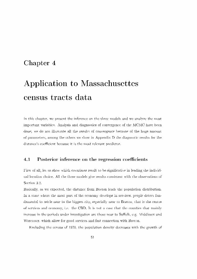
Chapter 4

Application to Massachusettes

census tracts data

In this chapter, we present the inference on the three models and we analyze the most

important variables. Analysis and diagnostics of convergence of the MCMC have been

done; we do not illustrate all the results of convergence because of the huge amount

of parameters, among the others we show in Appendix D the diagnostic results for the

distance's coecient because it is the most relevant predictor.

4.1 Posterior inference on the regression coecients

First of all, let us show which covariates result to be signicative in leading the individ-

ual location choice. All the three models give results consistent with the observations of

Section 3.2.

Basically, as we expected, the distance from Boston leads the population distribution.

In a state where the most part of the economy develops in services, people detect fun-

damental to settle near to the biggest city, especially near to Boston, that is the centre

of services and economy, i.e. the CBD. It is not a case that the counties that mainly

increase in the periods under investigation are those near to Suolk, e.g. Middlesex and

Worcester, which allow for good services and fast connection with Boston.

Excluding the census of 1970, the population density decreases with the growth of

51

Figure 4.1: Credibility intervals for the regression coecients at level 90%, under the baseline

model.

distance. It is worth to notice that, for almost all the covariates, in 1970 and 1980 a

dierent behavior appears in the estimations with respect to most recent years. As we

explained in the descriprion of the dataset, that is because the second but especially the

rst census were collected with dierent criterions; one can notice that even for other

variables in 1970 there is an evolution in opposition to the other times. Referring to

Figures 4.1, 4.2 and 4.3 (the estimation and the quantiles for the regressors β(t)h can be

found in Appendix C), we can state that modelling the individual choice only considering

the distance it would be restrictive. Also the ethnic composition plays a relevant role.

People prefer to move where there is a more proportion of white inhabitants, that should

guarantee the presence of wealthier people and a lower rate of criminality. Even the

economic indicator results to be important. It turns out that richer people, with an high

income, prefer to live far from the city, where there is a lower population density; in this

way they can own big properties. Insteed, if the income is equally distributed, the density

of population increases, as people place where there is a diused wellness. The education

52

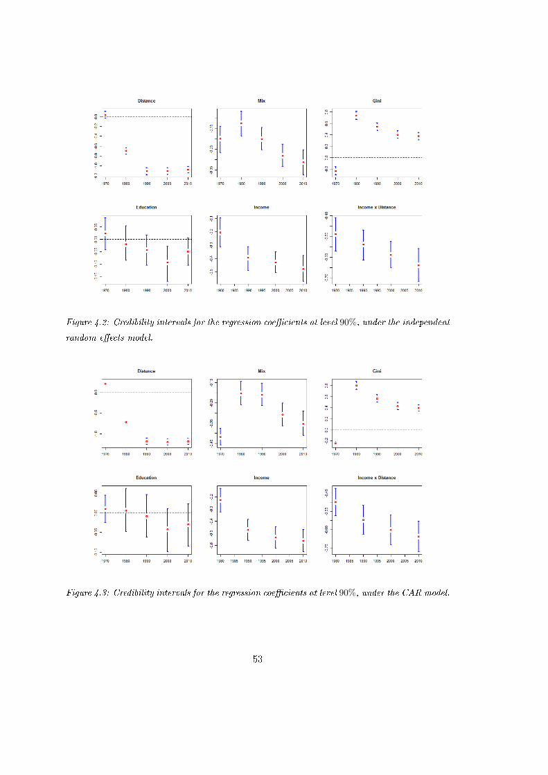
Figure 4.2: Credibility intervals for the regression coecients at level 90%, under the independent

random eects model.

Figure 4.3: Credibility intervals for the regression coecients at level 90%, under the CAR model.

53

level becomes important only in more recent time. It is interesting to notice that after

1990 the importance of the distance and the income inuence remain almost constant,

while the mix and the education factors become more and more relevant in a negative

way. On the other hand the Gini index looses inuence over time. These paths of the

coecients can be explained as an increase of the importance of the reputation eects:

people are more and more interested in the feature of the cities they have selected.

Since these estimation are quite similar in all the three models, we can conclude that

the introduction of spatial eects does not aect the dynamic trends of the regression

coecients.

4.2 Autocorrelation and heteroschedasticity

The study of spatial correlation is divided in two levels: the eect of belonging to a

county and the eect of the neighbourhood.

The county eect translates into two aspects: the regressor given by the amenities

and the variance's structure. The estimations for the amenities' coecients is reported in

Table 4.1. One can notice that, except for the rst year, the amenities are pratically non

inuencial neither in the baseline model nor in the independent random eects. Instead,

in the CAR model, b(t)1 is signicative in a negative way. This is a logical behavior since,

if the amenities are higher it means that the proportion of water area is extended and

hence the population density would be lower.

1970 1980 1990 2000 2010

Baseline model 0.43 0.12 0.02 0.06 0.11

(0.38,0.49) (0.07,0.18) (-0.04,0.07) (0.00,0.11) (0.06,0.16)

Indipendent model 0.43 0.12 0,00 0.03 0.09

(0.35,0.49) (0.06,0.17) (-0.05,0.05) (-0.01,0.08) (0.05,0.15)

CAR model −0.31 −0.29 −0.33 −0.34 −0.34

(-0.39,-0.22) (-0.37,-0.18) (-0.41,-0.25) (-0.43,-0.27) (-0.42,-0.25)

Table 4.1: Estimation of the coecient of the amenities β1 in the three models. We show the

mean ( it is highligth if the coecient results signicative) and the 2.5% and 97.5% quantiles.

54

The variances σ2ν of the log densities of population turn out to be dierent each

others. This variance structure really allows to capture the heteroschedasticity of the

data: the values obtained are dierent for each county, we can deduce that there is a

strong county eect.

Baseline model Indipendent model CAR model

Barnstable(1) 3.53 3.48 3.23

Hampshire(2) 10.07 8.26 6.41

Berkshire(3) 11.39 11.18 10.89

Middlesex(4) 3.82 1.94 1.17

Bristol(5) 5.25 3.39 2.56

Nantucket(6) 12.13 14.76 21.04

Dukes(7) 5.71 3.59 1.30

Norfolk(8) 2.63 1.35 0.81

Essex(9) 2.94 1.49 1.08

Plymouth(10) 4.87 3.36 1.86

Franklin(11) 9.51 8.30 5.57

Suolk(12) 3.22 2.28 2.21

Hampden(13) 7.62 7.25 7.33

Worcester(14) 7.50 5.31 3.71

Table 4.2: Estimation of the variances σ2ν of the population densities under the three alternative

models.

The estimations obtained in the three dierent cases are perfectly consistent to each

others. As the estimations in the CAR model were not precise, then we correct them by

means of the other models estimations. We can divide the counties in two main groups.

One one side, we have all these counties with a large number of census tracts, like Mid-

dlesex or Suolk; in this case the variances are low, and the corresponding intervals of

credibility is narrow (see Figures 4.4, 4.5 and 4.6). Actually in a very populous county

there is a homogeneous population distribution, so there are no big dierences. On the

other hand, we expect that in a county with a little number of census tracts there would

55

be more dierences inside the county, due to the extended area of a census tract that

includes dierent situations. We nd validation to our observation in the obtained esti-

mations, indeed, counties as Dukes or Franklin have higher variability than to the other

counties. Even though the behaviors of the variances are quite similar, anyway, adding

spatial eects make the estimation more precise (see Table 4.2).

Figure 4.4: Credibility intervals of the variances of the density population Y on log scale at level

90%, under the baseline model.

56

Figure 4.5: Credibility intervals of the variances of the density population Y on log scale at level

90%, under the random independent eects model.

Figure 4.6: Credibility intervals of the variances of the density population Y on log scale at level

90%, under the CAR model.

Let us now investigate the local spatial correlation. The maps in Figures 4.7-4.11

show the dynamic evolution of the spatial independent random eects. One can notice

that in the rst two periods the random eects are signicant, while, time after time, the

estimations of the random eects approach zero for every census tracts. We expected

57

this behavior because the number of census tracts is increasing over time, whereas as one

can see in Figure 3.6 the density of a single census tract keeps almost constant, but the

area becomes smaller over time. This lead to a homogeneus behavior of the population

density in the single unit, the variability is all described by the covariates and there is no

need of additional eects to interpretate the phenomenon. Concerning the census tracts

in the country area, we notice that in the past the correspponding spatial independent

random eects are signicantly negative, whereas in more recent time they become null.

This fact can be due to the improvement of transportation during the years. so that

people can easily commute to Boston. On the other, the random eect on the census

tracts in the big cities tend to be positive. The diernt sign of the random eects in the

countryside with respect to the urban areas shows that actually there is a relevant part

of the variability of the population density unexplained by the covariate.

Figure 4.7: Estimation of the independent spatial random eects in 1970.

58

Figure 4.8: Estimation of the independent spatial random eects in 1980.

Figure 4.9: Estimation of the indipendt spatial random eects in 1990.

59

Figure 4.10: Estimation of the indipendt spatial random eects in 2000.

Figure 4.11: Estimation of the indipendt spatial random eects in 2010.

60

1970 1980 1990 2000 2010

ρ 0.99 0.72 0.57 0.50 0.53

(0.99,0.99) (0.57,0.84) (0.37,0.72) (0.27,0.70) (0.30,0.72)

Table 4.3: Estimation of ρ . We show the mean and the (2.5%,97.5%) quantiles.

From the analysis of the CAR model results, we know that there is spatial correlation

among the census tracts. Referring to Table 4.3, the estimations of ρ represent the

strenght of the autocorrelation, hence in 1970 and 1980 the spatial dependence is stronger

than in the other periods. Anyway there is always positive spatial dependence among

data. Maps in Figures 4.12-4.16 show the dynamic evolution of the random eects. Under

the CAR specication on the random eects, the interpretation of the estimated random

eects is not as clear as in the independent case. For example in 1990s Φ(t) are almost

null, whereas 20 years later in 2010 they become almost all negative as one can see in

Figures 4.13-4.14. Some furter investigations are required.

Figure 4.12: Estimation of the spatial random eects under the CAR model in 1970.

61

Figure 4.13: Estimation of the spatial random eects under the CAR model in 1980.

Figure 4.14: Estimation of spatial random eects under the CAR model in 1990.

62

Figure 4.15: Estimation of spatial random eects under the CAR model in 2000.

Figure 4.16: Estimation of the spatial random eects under the CAR model in 2010.

63

Finally, let us explore the estimations of the varinces of the random eects under

both independent and CAR random eects models. Using the formula for the variance

decomposition:

V ar(log(Y(t)j )) = V ar(E[log(Y

(t)j )|φ(t)

j ]) + E[V ar(log(Y(t)j )|φ(t)

j )] ,

one can show that

V ar(Y(t)j |β

(t)j , ρ(t), τ (t), σ2, νi[j]) ∝ cjτ (t) + σ2νi[j]

where

cj ∝

1 under independent random model for φ

(t)j

1

n(t)j

under CAR model for φ(t)j .

Hence, the variance of the random eects inuences the variance of the population den-

sity. Both λ(t) and τ (t) show the same trend, the values estimated decreasing over time.

All in all, the idea that emerges from the analysis is that over time there is a progressive

homogeneity in population distribution. Census tracts eects are going to zero, and the

population density is almost constantly distributed in the countryside (see Figure 3.6).

Figure 4.17: Credibility intervals of the common term λ(t) in the variances of the spatial random

eects model at level 90%, under the random independent eects model. Credibility intervals

of the common term τ (t) in the variances of the spatial random eects at level 90%, under the

random CAR model.

64

4.3 Models comparison

In this section we compare the results obtain in the three models. First of all an index

for the goodness-of-t of the model has to be introduced. In this work, we choosed the

Log Pseudo Marginal Likelihood (LPML) in order to evaluate the performances of the

models and compare them. The LPML is dened as the sum of the logarithms of the

Conditional Predictive Ordinates (CPO) for each observation, i.e.

LPML =

N∑i=1

log(CPOi) ,

where CPOi is the value of the predictive distribution evaluated at yi, conditional to the

training sample y−i not containing the i-th observation. This approach is very common

in the cross validation techniques, when the data matrix is partitioned in two parts:

one is used to estimate the parameters, and the other to measure the goodness of t.

Obviously, the larger the value of the CPO (and, subsequently, of the LPML) is, the

better the model prevision is. The calculation of LPML consists in the evaluation of n

predictive distributions, which can be computationally heavy. However, an alternative

formula can be proved for CPOi = fi(yi|y−i). In fact

CPOi = fi(yi|y−i) =

∫Θfi(yi|θ)L(dθ|y−i) =

=

∫Θfi(yi|θ)

∏j 6=i

fj(yj |θ)L(θ)dθ∫Θ

∏j 6=i

fj(yj |θ)L(θ)dθ,

and using the Bayes' theorem we obtain:

CPO−1i =

∫Θ

∏j 6=i

fj(yj |θ)L(dθ)

∫Θ

n∏i=1

fi(yi|θ)L(dθ)

=

=

∫Θ

1

fi(yi|θ)

n∏i=1

fi(yi|θ)L(dθ)∫Θ

n∏i=1

fi(yi|θ)L(dθ)

=

∫Θ

1

fi(yi|θ)L(dθ|y) .

In the light of the ergodic theorem, the las integral can be approximated by:

CPO−1i =

1

M

M∑m=1

1

fi(yi|θ(m)),

65

where M is the number of iterations and θ(m) is the value of the chain at iteration m.

The estimated values of the LPML index for every model are listed in Table 4.4.

1970 1980 1990 2000 2010 TOT

Baseline model -2258 -2221 -2335 -2394 -2599 -11807

Indipendent model -1908 -1951 −2050 −2114 −2302 -10325

CAR model −1745 −1816 -2206 -2150 -2311 −10228

Table 4.4: LPML values for every years.

According to LPML criterion, both the models with spatial eects perform better

than the baseline model, and they have similar performance since the values are almost

the same.

As further measure of goodness of t and comparison of the models, we calculate the

outliers of the models. The outliers are determined by means of the bayesian predictive

p-values. In a Bayesian context, the posterior (or predictive) p-value is the probability,

given the data, that a future observation is more extreme than the data. Mathemati-

cally, a Bayesian p-value can be computed by averaging over the distribution of p-values

(with distribution induced by uncertainty about unknown parameters); see, for example,

Gelman, Meng and Stern (1996) and Bayarri and Berger (2000). Pratically, we compute

the predictive value for each census tract, given by

y(m)i = f(y

(t)i |θ

(m)), t = 1, . . . , 5,m = 1, . . . ,M

where M is the number of iterations and θ(m) is the value of the chain at iteration m.

Once y(t)i has been obtained, we compute the the numberM1 of data such that y

(m)i < y

(t)i

and M2 such that y(m)i > y

(t)i . Hence the predictive p-value is computed as follows:

p.loweri =M1

M

p.upperi =M2

M

p_valuei = min(p.upperi, p.loweri)

The predictive p-value ranges between 0.5 and 0, it il is close to zero it means that the

actual datum is in the tails of the posterior distribution, hence it is not well explained

66

by the model. In this work we consider as outliers those data with a p-value lower than

0.1.

The percentage of outliers in each model are listed in Table 4.5.

Even if the CAR model has more outlier than the others, anyway all the models t well

1970 1980 1990 2000 2010

Baseline model 0.05 0.02 0.01 0.005 0.004

Indipendent model 0 0.007 0.004 0.004 0.005

CAR model 0.002 0.01 0.06 0.05 0.04

Table 4.5: Percentage of outliers for every years.

the observations. The grahs of the predictions in the independent random eects model

and in the CAR model in 2010 are shown in Figures 4.16 and 4.17 The predictions of the

models t perfectly the data.

Figure 4.18: Predicted and actual log-density of population in 2010 under independet random

eects model.

67

Figure 4.19: Predicted and actual log-density of population in 2010 under CAR model.

68

Chapter 5

Concluding Remarks

In this thesis we have applied three dierent dynamic Bayesian hierarchical regression

lognormal models to population density at level of census tracts; we have compared the

results to study spatial and time correlation among data of Massachusetts census tracts.

Time dipendence has been introduced by an autoregressive structure on the regression

coecients. The spatial random eects take account for spatial correlation. As we ex-

pected, we found out that the reputation of a place plays an important role in inuencing

the individual decision. People prefer to settle in a wellness place, characterize by a good

economic situation and similar ethnic composition. Anyway the distance from Boston

remains the most important feature in leading population trend over time.

A remarkable result is that the introduction of spatial random eects improve the pre-

dictions of the actual population densities: it seems that it is sucient to introduce

independent random eects to better capture the population densities' variability. In

addition, the Bayesian inference of the CAR model highlight an eective dependence by

the neighbours features. It is worth to underline that the estimations for the regression

coecients are quite similar under baseline, independent and CAR random eects model.

69

70

Appendices

71

Appendix A

Full conditionals calculation

The calculus of the full conditional distributions are explained in details. Given the

posterior distribution relative to the CAR model

β(0),β(1), . . . ,β(5), σ2,ν,Φ(1), . . . ,Φ(5),Σβ, τ(1), . . . , τ(5), . . .

. . . , ρ(1), . . . , ρ(5)|Y (1), . . . ,Y (5), V (1), . . . , V (5)

∝5∏t=1

[π(Y (t)|β(t),ν, σ2,Φ(t), V (t))]π(β(1), . . . ,β(5)|β(0),Σβ)π(β(0))π(Σβ)π(σ2)π(ν)×

×5∏t=1

[π(Φ(1), . . . ,Φ(5)|ρ(t), τ (t))π(ρ(t))π(τ (t))]

∝5∏t=1

[π(Y (t)|β(t),ν, σ2,Φ(t), V (t))π(Φ(1), . . . ,Φ(5)|ρ(t), τ (t))π(ρ(t))π(τ t)π(β(t)|β(t−1),Σβ)]×

× π(ν)π(Σβ)π(σ2)π(β(0))π(ρ(t))π(τ (t))

we can compute the full conditionals for each parameters.

Update of regressiors coecients

The update of the the regression coecients depend on the time.

For t = 0

β(0)|β(1),Σβ ∝ π(β(1)|β(0),Σβ)π(β(0))

∝ exp−1

2(β(1) − β(0))′Σ−1

β (β(1) − β(0))

exp

− 1

200(β(0))′β(0)

.

73

Since the covariance matrix is diagonal, we can factorize the distribution, for h = 1, . . . , 8

β(0)h |β

(1)h , σ2

βi∝ exp

− 1

2σ2βh

(β(1)h − β

(0)h )2

exp

− 1

200(β

(0)i )2

∝ exp

−1

2

[(β

(0)h )2

(1

σ2βh

+1

100

)− 2β

(0)h

β(1)h

σ2βh

]therefore

β(0)h |β

(1)h , σβh ∼ N

( 1

σ2βh

+1

100

)−1β

(1)h

σ2βh

,

(1

σ2βh

+1

100

)−1

For t = 1, 2, 3, 4 the distribution depends on both the previous and the next values

of β, we dene the diagonal matrix N such that Ni,i = νi[j]. As in the case above the

distribution can be factorized, hence for h = 1, . . . , 8

β(t)h |β

(t−1)h , β

(t+1)h ,Φ(t), σ2

βi,ν,Y (t), V (t), σ2

∝ π(Y (t)|β(t),ν, σ2,Φ(t), V (t))π(β(t)|β(t−1),Σβ)π(β(t+1)|β(t),Σβ)

∝ exp

− 1

2σ2(Y (t) − V (t)

h β(t)h −

∑k 6=h

V(t)k β

(t)k −Φ(t))′N−1(Y (t) − V (t)

h β(t)h −

∑k 6=h

V(t)k β

(t)k −Φ(t))

×× exp

− 1

2σ2βh

(β(t)h − β

(t−1)h )2

exp

− 1

2σ2βh

(β(t+1)h − β(t)

h )2

∝J [t]∏j=1

exp

− 1

2σ2νi[j](y

(t)j − V

(t)h,j β

(t)h −

∑k 6=h

V(t)k,j β

(t)k − φ

(t)j )2

×× exp

− 1

2σ2βh

(β(t)h − β

(t−1)h )2

exp

− 1

2σ2βh

(β(t+1)h − β(t)

h )2

by dening the quantities

k(t) = y(t)j −

∑k 6=h

V(t)k,j β

(t)k − φ

(t)j

we rewrite

exp

− 1

2σ2

(β(t)h )2

J [t]∑j=1

(V(t)h,j )2

νi[j]− 2β

(t)h

J [t]∑j=1

V(t)h,j k

(t)

νi[j]

− 1

2σ2βh

[2(β

(t)h )2 − 2β

(t)h (β

(t+1)h + β

(t−1)h )

]∝ exp

−1

2

(β(t)h )2

1

σ2

J [t]∑j=1

(V(t)h,j )2

νi[j]+

2

σ2βh

− 2β(t)h

1

σ2

J [t]∑j=1

V(t)h,j k

(t)

νi[j]+

1

σ2βh

(β(t+1)h + β

(t−1)h )

.

74

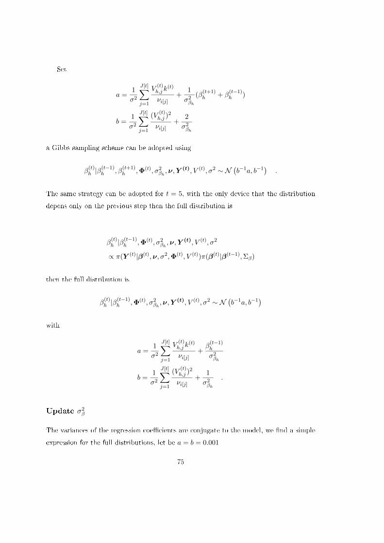
Set

a =1

σ2

J [t]∑j=1

V(t)h,j k

(t)

νi[j]+

1

σ2βh

(β(t+1)h + β

(t−1)h )

b =1

σ2

J [t]∑j=1

(V(t)h,j )2

νi[j]+

2

σ2βh

a Gibbs sampling scheme can be adopted using

β(t)h |β

(t−1)h , β

(t+1)h ,Φ(t), σ2

βh,ν,Y (t), V (t), σ2 ∼ N

(b−1a, b−1

).

The same strategy can be adopted for t = 5, with the only device that the distribution

depens only on the previous step then the full distribution is

β(t)h |β

(t−1)h ,Φ(t), σ2

βh,ν,Y (t), V (t), σ2

∝ π(Y (t)|β(t),ν, σ2,Φ(t), V (t))π(β(t)|β(t−1),Σβ)

then the full distribution is

β(t)h |β

(t−1)h ,Φ(t), σ2

βh,ν,Y (t), V (t), σ2 ∼ N

(b−1a, b−1

)with

a =1

σ2

J [t]∑j=1

V(t)h,j k

(t)

νi[j]+β

(t−1)h

σ2βh

b =1

σ2

J [t]∑j=1

(V(t)h,j )2

νi[j]+

1

σ2βh

.

Update σ2β

The variances of the regression coecients are conjugate to the model, we nd a simple

expression for the full distributions, let be a = b = 0.001

75

σ2βh|β(1)h , . . . , β

(5)h ∝

5∏t=1

π(β(t)h |β

(t−1)h , σ2

βh)π(σ2

βh)

∝5∏t=1

[1

(σ2βh

)1/2exp

−

(β(t)h − β

(t−1)h )2

2σ2βh

]1

(σ2βh

)a+1exp

− b

σ2βh

I[0,∞](σ

2βh

)

∝ 1

(σ2βh

)5/2+a+1exp

−5∑t=1

(β(t)h − β

(t−1)h )2 + 2b

2σ2βh

I[0,∞](σ2βh

)

we nd

σ2βh|β(1)h , . . . , β

(5)h ∼ IG

a+5

2, b+

5∑t=1

(β(t)h − β

(t−1)h )2

2

∀h = 1, . . . , 8 .

Update σ2

The variance σ2 is simply updated with an inverse-gamma ditribution with hyperparam-

eters a = b = 0.001

σ2|β(1)i , . . . ,β

(5)i ,ν,Φ(1), . . . ,Φ(5),Y (1), . . . ,Y (5), V (1), . . . , V (5)

∝5∏t=1

π(Y (t)|β(t),ν, σ2, φ(t)j , V

(t))π(σ2)

∝5∏t=1

[1

(σ2)J [t]/2exp

− 1

2σ2(Y (t) − V (t)β(t) −Φ(t))′N−1(Y (t) − V (t)β(t) −Φ(t))

]×

× 1

(σ2)a+1exp

− b

σ2

I[0,∞](σ

2)

∝ 1

(σ2)

5∑t=1

J [t]/2+a+1

exp

−5∑t=1

(Y (t) − V (t)β(t) −Φ(t))′N−1(Y (t) − V (t)i β(t) −Φ(t)) + 2b

2σ2

I[0,∞](σ2)

76

so we obtain

σ2|β(1), . . . ,β(5),ν,Φ(1), . . . ,Φ(5),Y (1), . . . ,Y (5), V (1), . . . , V (5) ∼

∼ IG

a+

5∑t=1

J [t]

2, b+

5∑t=1

(Y (t) − V (t)β(t) −Φ(t))′N−1(Y (t) − V (t)β(t) −Φ(t))

2

.

Update ν

Since ν1, . . . , ν14 are independent, the dataset and the parameters can be partitioned in

this way: Y(t)i , V

(t)i ,Φ

(t)i are the data and the parameters relative to i− th county.

For i = 1, . . . , 14, let ber = 4 and the diagonal matrix N such that Ni,i = nui[j].

Let us write the determinat of N as follow

|N |1/2 =

n(t)1∏j=1

ν1 · · ·n(t)i∏j=1

νi · · ·n(t)14∏j=1

ν14

1/2

∝ νn(t)i /2

i .

Therefore the conditional distribution is

νi|β(1), . . . ,β(5), σ2,Φ(1)i , . . . ,Φ

(5)i ,Y

(1)i , . . . ,Y

(5)i , V

(1)i , . . . , V

(5)i

∝5∏t=1

π(Y(t)i |β

(t), νi, σ2,Φ

(t)i , V

(t)i )π(νi)

∝5∏t=1

1

νn(t)i /2

i

exp

− 1

σ2νi(Y

(t)i − V (t)

i β(t) −Φ(t)i )′(Y

(t)i − V (t)

i β(t) −Φ(t)i )

×× 1

(νi)r/2+1exp

− r

2νi

I[0,∞](νi)

∝ 1

(νi)

5∑t=1

n(t)i /2+r/2+1

×

× exp

− 1

νi

(5∑i=1

(Y(t)i − V (t)

i β(t) −Φ(t)i )′(Y

(t)i − V (t)

i β(t) −Φ(t)i )

2σ2+r

2

)I[0,∞](νi)

by dening the quantities

k(t) =(Y

(t)i − V (t)

i β(t) −Φ(t)i )′(Y

(t)i − V (t)

i β(t) −Φ(t)i )

2σ2

77

we obtain for all i = 1, . . . , 14

νi|β(1), . . . ,β(5), σ2,Φ(1)i , . . . ,Φ

(5)i ,Y

(1)i , . . . ,Y

(5)i , V

(1)i , . . . , V

(5)i ∼

∼ IG

r2 +

5∑t=1

n(t)i

2,r

2+

5∑i=1

k(t)

.

Update τ (t)

The hyperparameters fot τ (t) are a = 0.5 and b=0.005. As the other variances prior,

even in this case it is a conjugate prior, hence the full conditional distribution is simply

τ (t)|Φ(t), ρ(t) ∝ π(Φ(t)|ρ(t), τ (t))π(τ (t))

∝ 1

(τ (t))J [t]/2exp

− 1

2τ (t)(Φ(t))′(D(t)

w − ρ(t)W (t))Φ(t)

1

(τ (t))a+1exp

− b

τ (t)

I[0,∞](τ

(t))

∝ 1

(τ (t))a+J [t]/2+1exp

− 1

τ (t)

[b+

(Φ(t))′(D(t)w − ρ(t)W (t))Φ(t)

2

]I[0,∞](τ

(t))

τ (t)|Y (t), V (t),Φ(t), ρ(t) ∼ IG

(a+

J [t]

2, b+

(Φ(t))′(D(t)w − ρ(t)W (t))Φ(t)

2

)

Update ρ(t)

In order to sample from the full conditional distribution we need the relation between

the eigenvalues of matrix A(t) and I − ρ(t)A(t). Let µ(t)j be the eigenvalues of I − ρ(t)A(t)

and λ(t)i be the eigenvalues of A(t), then the following holds

µ(t)j = 1− ρ(t)λ

(t)j

for the demostration we recall Section 3.3 . Hence the determinant of I − ρ(t)A(t) can be

written as

|(I−ρ(t)A(t))−1D|1/2 = |I−ρ(t)A(t)|−1/2|D|1/2 ∝

J [t]∏j=1

µ(t)j

−1/2

∝

J [t]∏j=1

(1− ρ(t)λ(t)j )

−1/2

.

78

The full conditional distribution for ρ(t) is

ρ(t)|Φ(t), τ (t) ∝ π(Φ(t)|ρ(t), τ (t))π(τ (t))

∝ 1

|(I − ρ(t)A(t))−1D|1/2exp

− 1

2τ (t)(Φ(t))′D−1(I − ρ(t)A(t))Φ(t)

I[0,1](ρ

(t))

∝

J [t]∏j=1

(1− ρ(t)λ(t)j )

1/2

exp

1

2τ (t)ρ(t)(Φ(t))′D−1A(t)Φ(t)

I[0,1](ρ

(t)).

This distribution is unknown, so we sample with a step of Metropolis Hastings algorithm.

Update random eect parameters

We want to determine the full conditional distribution for Φ(t)

Φ(t)|Y (t), V (t),ν, σ2,β(t), τ (t), ρ(t) ∝ π(Y (t)|β(t),ν, σ2,Φ(t), V (t))π(Φ(t)|τ (t), ρ(t))

∝ exp

(Y (t) − V (t)β(t) −Φ(t))′N−1(Y (t) − V (t)β(t) −Φ(t))

2σ2

exp

−1

2(Φ(t))′

D(t)w − ρ(t)W (t)

τ (t)Φ(t)

∝

−1

2

[(Φ(t))′

N−1

σ2Φ(t) − 2(Φ(t))′

N−1

σ2(Y (t) − V (t)β(t)) + (Φ(t))′

D(t)w − ρ(t)W (t)

τ (t)Φ(t)

]

∝

−1

2

[(Φ(t))′

(N−1

σ2+D

(t)w − ρ(t)W (t)

τ (t)

)Φ(t) − 2(Φ(t))′

N−1

σ2(Y (t) − V (t)β(t))

]

hence this is the kernel of a multinormal distribution with parameters updated as

follow

Φ(t)|Y (t), V (t),ν, σ2,β(t), τ (t), ρ(t) ∼

∼MN

(N−1

σ2+D

(t)w − ρ(t)W (t)

τ (t)

)−1N−1

σ2,

(N−1

σ2+D

(t)w − ρ(t)W (t)

τ (t)

)−1 .

Since sampling from a multinormal distribution of such dimension is computationally slow

and some numeric error could occur, we propose a second full conditional distribution

obtained startinf from Equation 1.9. We condition the previos distribution with respect

79

to Φ(t)j and then the Bayes' theorem is applied

π(φ(t)j |Φ

(t)−j ,Y

(t), V (t),ν, σ2,β(t), τ (t), ρ(t))

=π(Y (t),ν, σ2,β(t), τ (t), ρ(t)|φ(t)

j ,Φ(t)−j)π(φ

(t)j |Φ

(t)−j)

π(Y (t),ν, σ2,β(t), τ (t), ρ(t)|Φ(t)−j)

∝ π(Y (t)|Φ(t))π(φ(t)j |Φ

(t)−j) .

Therefore we use the simpler full conditionals

φ(t)j |Φ

(t)−j , y

(t)j , V

(t)j , νi[j], σ

2,β(t), τ (t), ρ(t) ∼ N (b−1a, b−1)

where

b =1

σ2νi[j]+n

(t)j

τ (t)

a =y

(t)j − V

(t)j β(t)

σ2νi[j]+n

(t)j ρ

(t)A(t)j Φ(t)

τ (t).

80

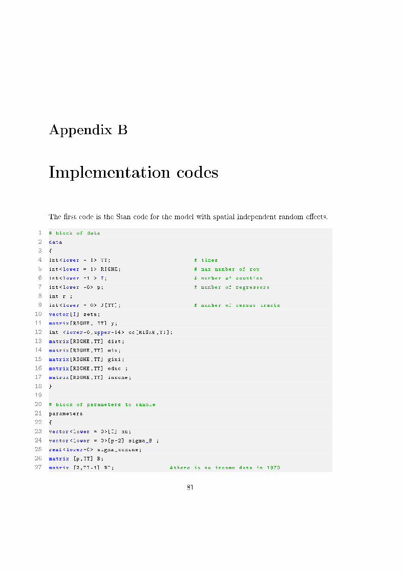
Appendix B

Implementation codes

The rst code is the Stan code for the model with spatial independent random eects.

1 # block of data

2 data

3

4 int <lower = 1> TT; # times

5 int <lower = 1> RIGHE; # max number of row

6 int <lower =1 > I; # number of counties

7 int <lower =0> p; # number of regressors

8 int r ;

9 int <lower = 0> J[TT]; # number of census tracts

10 vector[I] zeta;

11 matrix[RIGHE , TT] y;

12 int <lower=0,upper =14> cc[RIGHE ,TT];

13 matrix[RIGHE ,TT] dist;

14 matrix[RIGHE ,TT] mix;

15 matrix[RIGHE ,TT] gini;

16 matrix[RIGHE ,TT] educ ;

17 matrix[RIGHE ,TT] income;

18

19

20 # block of parameters to sample

21 parameters

22

23 vector <lower = 0>[I] nu;

24 vector <lower = 0>[p+2] sigma_B ;

25 real <lower=0> sigma_comune;

26 matrix [p,TT] B;

27 matrix [2,TT -1] BI; #there is no income data in 1970

81

28 vector [p+2] valori_iniziali;

29

30 vector[J[1]] phi1;

31 vector[J[2]] phi2;

32 vector[J[3]] phi3;

33 vector[J[4]] phi4;

34 vector[J[5]] phi5;

35 vector[TT] sigma_phi;

36

37 #block for the operations

38 transformed parameters

39 vector[I] sigma ;

40 matrix [RIGHE ,TT] media_beta;

41 matrix[RIGHE ,TT] media_comune;

42

43 for (i in 1:I) sigma[i] <- pow(nu[i],0.5)*pow(sigma_comune ,0.5)*pow(r,-0.5);

44

45 for(j in 1:J[1])

46 media_beta[j,1] <-dist[j,1]*B[3,1]+ mix[j,1]*B[4,1] + gini[j,1]*B[5,1] + educ[j,1]*

B[6 ,1];

47

48

49 for(t in 2:TT)

50 for(j in 1:J[t])

51 media_beta[j,t]<-dist[j,t]*B[3,t]+ mix[j,t]*B[4,t] + gini[j,t]*B[5,t]+ educ[j,t]*B

[6,t]+ income[j,t]*BI[1,t-1]+ income[j,t]*dist[j,t]*BI

[2,t-1];

52

53

54 for(t in 1:TT)

55 for(j in 1:J[t]) media_comune[j,t]<-B[1,t]+ B[2,t]* zeta [cc[j,t]];

56

57

58 model

59

60 # Prior:

61 # 1) variance prior

62 sigma_comune ~ inv_gamma (0.001 , 0.001);

63

64 for (i in 1:(p+2))

65 sigma_B[i] ~ uniform (0.001 ,10);

66

67 for (i in 1:I)

68 nu[i] ~ chi_square (r);

82

69

70 # 2) AR(1)

71 for (i in 1:(p+2))valori_iniziali[i]~ normal (0,pow (10 ,0.5));

72

73 for (i in 1:p)

74 B[i,1]~ normal(valori_iniziali[i],sigma_B[i]);

75 for (t in 2:TT)

76 B[i,t]~ normal(B[i,t-1],sigma_B[i]);

77

78 for (i in 1:2)

79 BI[i,1]~ normal(valori_iniziali[i+6], sigma_B[i+6]);

80 for (t in 2:4)

81 BI[i,t]~ normal(BI[i,t-1], sigma_B[i+6]);

82

83

84 #3) independent random effects

85 for (t in 1:TT) sigma_phi[t] ~ inv_gamma (0.001 , 0.001);

86

87 for(i in 1:J[1]) phi1[i] ~ normal(0,pow(sigma_phi [1] ,0.5));

88 for(i in 1:J[2]) phi2[i] ~ normal(0,pow(sigma_phi [2] ,0.5));

89 for(i in 1:J[3]) phi3[i] ~ normal(0,pow(sigma_phi [3] ,0.5));

90 for(i in 1:J[4]) phi4[i] ~ normal(0,pow(sigma_phi [4] ,0.5));

91 for(i in 1:RIGHE) phi5[i] ~ normal(0,pow(sigma_phi [5] ,0.5));

92

93 # Likelihood:

94 for (j in 1:J[1])

95 y[j,1] ~ lognormal(media_beta[j,1]+ phi1[j]+media_comune[j,1] , sigma[cc[j,1]] );

96 for (j in 1:J[2])

97 y[j,2] ~ lognormal(media_beta[j,2]+ phi2[j]+media_comune[j,2] , sigma[cc[j,2]] );

98 for (j in 1:J[3])

99 y[j,3] ~ lognormal(media_beta[j,3]+ phi3[j]+media_comune[j,3] , sigma[cc[j,3]] );

100 for (j in 1:J[4])

101 y[j,4] ~ lognormal(media_beta[j,4]+ phi4[j]+media_comune[j,4] , sigma[cc[j,4]] );

102 for (j in 1:J[5])

103 y[j,5] ~ lognormal(media_beta[j,5]+ phi5[j]+media_comune[j,5] , sigma[cc[j,5]] );

104

105

83

The second code is written in Julia, it is the implemenatation of the CAR model. For

this second one we do not shown all the code, only the most important parts.

The functions for sampling from the full distribution of the regression coecient, the

variance of the coecients and the variable ρ are reported:

1

2 #update of regression coefficients

3

4 function upd_b0(beta , sigma_beta , j, diago , sigma_y, y , p ,shift)

5 d =length(beta)

6 out=zeros(Float64 ,d)

7 var =1./(1./sigma_beta +1/ 100)

8 med=var*beta [2]./sigma_beta

9 out [1]= rand(Normal(med ,var) ,1)[]

10

11 for t in 2:(d-1)

12 temp= diago [1:J[t-shift],t-shift]

13 b_inv = 1/(sum(temp)/sigma_y + 2/sigma_beta)

14 a=dot(temp ,y[1:J[t-shift],t-shift]-p[1:J[t-shift],t-shift])./sigma_y + (out[t-1]+

beta[t+1])./sigma_beta

15 out[t]=rand(Normal(b_inv*a,b_inv) ,1)[]

16 end

17

18 t=d

19 temp= diago [1:J[t-shift],t-shift]

20 b_inv = 1/(sum(temp)/sigma_y + 1/sigma_beta)

21 a=dot(temp ,y[1:J[t-shift],t-shift]-p[1:J[t-shift],t-shift])./sigma_y + out[t-1]./

sigma_beta

22 out[t]=rand(Normal(b_inv*a,b_inv) ,1)[]

23

24 return(out)

25 end;

26

27 function upd_beta(beta , data , sigma_beta , j, diago , sigma_y,y,p,shift)

28 d = length(beta)

29 out=zeros(Float64 ,d)

30 var=1/(1./sigma_beta +1/ 100)

31 med=var*beta [2]/sigma_beta

32 out [1]= rand(Normal(med ,var) ,1)[]

33 for t in 2:(d-1)

34 temp= data [1:J[t-shift],t-shift ].*diago [1:J[t-shift],t-shift]

35 b_inv = 1/(dot(temp ,data [1:J[t-shift],t-shift])./sigma_y + 2/sigma_beta)

84

36 a=dot(temp ,y[1:J[t-shift],t-shift]-p[1:J[t-shift],t-shift])./sigma_y + (out[t-1]+

beta[t+1])./sigma_beta

37 out[t]=rand(Normal(b_inv*a,b_inv) ,1)[]

38 end

39

40 t=d

41 temp= data [1:J[t-shift],t-shift ].*diago [1:J[t-shift],t-shift]

42 b_inv = 1/(dot(temp ,data [1:J[t-shift],t-shift])./sigma_y + 1/sigma_beta)

43 a= dot(temp ,y[1:J[t-shift],t-shift]-p[1:J[t-shift],t-shift ])./sigma_y + out[t-1]./

sigma_beta

44 out[t]=rand(Normal(b_inv*a,b_inv) ,1)[]

45

46 return(out)

47 end;

1 function logfun(x,p,M,aut ,t)

2 temp=sum(log(1 - x*aut));

3 out = 0.5*temp - 0.5*(x/t)*transpose(p)*M*p

4 return(out)

5 end;

6 function upd_rho ( r, phi ,M,aut ,t)

7 out = r

8 delta = rand(Uniform (0,1), 1) [] # campiono da proposal

9 acp = logfun(delta ,phi ,M,aut ,t)-logfun(r,phi ,M,aut ,t)

10 acp = minimum ([0.0 , acp []])

11 ta = log(rand(Uniform (0,1) ,1)[])

12 if ta < acp

13 out = delta

14 end

15 return (out)

16 end;

17

18 function sigma_beta(a_sigma ,b_sigma , b)

19 temp=0

20 temp=sum((b[2:end]-b[1:(end -1)]).^2)

21 out = rand(InverseGamma(a_sigma , b_sigma + 0.5*temp),1 )[]

22 end;

The Gibbs sampling algorithm has been implemented as follow

1 #Gibbs

2

3 for k in 1:n_iter

4 t=1

5 TR[1:J[t],t]=y[1:J[t],t]-b0[t+1]-b1[t+1]*z[1:J[t],t]-beta_dist[t+1]*dist [1:J[t],t

]-beta_mix[t+1]*mix[1:J[t],t]-beta_gini[t+1]*gini [1:J[t],t]-

85

6 beta_educ[t+1]*educ [1:J[t],t]-phi [1:J[t],t]

7

8 for t in 2:TT

9 TR[1:J[t],t]=y[1:J[t],t]-b0[t+1]-b1[t+1]*z[1:J[t],t]-beta_dist[t+1]*dist [1:J[t],t

]-beta_mix[t+1]*mix[1:J[t],t]-beta_gini[t+1]*gini [1:J[t],t]-

10 beta_educ[t+1]*educ [1:J[t],t]-beta_income[t]*income [1:J[t],t]-beta_income_dist[t]*

L[1:J[t],t]-phi[1:J[t],t]

11 end

12 #update nu -------------------------------------------------------------------

13 for i in 1:14

14 b=0

15 for t in 1:TT

16 b=b+sum(TR[indici_contea[i,1:n_i[i,t],t],t].^2)

17 end

18 nu[i]=rand(InverseGamma(a_nu[i],(b_nu+0.5*b/sigma_y)[]) ,1)[]

19 end

20

21 #update sigma_y --------------------------

22 for t in 1:TT

23 diago [1:J[t],t]=1./nu[cc[1:J[t],t]]

24 end

25

26 K = 0

27 for t in 1:TT

28 #K=K+ transpose(TR[1:J[t],t])*(diago [1:J[t],t].*TR[1:J[t],t])

29 K=K+dot(TR[1:J[t],t],diago [1:J[t],t].*TR[1:J[t],t])

30 end

31 sigma_y = rand(InverseGamma(a_sigma_y,b_sigma_y + 0.5*K) ,1)[]

32 ## update beta e sigma_beta -------------------------------------

33 sigma_beta_dist = sigma_beta(a_sigma_beta ,b_sigma_beta , beta_dist);

34 sigma_b0 = sigma_beta(a_sigma_beta ,b_sigma_beta , beta_dist);

35 sigma_b1 = sigma_beta(a_sigma_beta ,b_sigma_beta , beta_dist);

36 sigma_beta_mix = sigma_beta(a_sigma_beta ,b_sigma_beta , beta_mix);

37 sigma_beta_gini = sigma_beta(a_sigma_beta ,b_sigma_beta , beta_gini);

38 sigma_beta_educ = sigma_beta(a_sigma_beta ,b_sigma_beta , beta_educ);

39 sigma_beta_income = sigma_beta(a_sigma_beta ,b_sigma_beta , beta_income);

40 sigma_beta_income_dist = sigma_beta(a_sigma_beta ,b_sigma_beta , beta_income_dist);

41

42 t=1

43 delta [1:J[t],t]=y[1:J[t],t]-b1[t+1]*z[1:J[t],t]-beta_dist[t+1]*dist [1:J[t],t]-beta

_mix[t+1]*mix[1:J[t],t]-beta_gini[t+1]*gini [1:J[t],t]-

44 beta_educ[t+1]*educ [1:J[t],t]-phi [1:J[t],t]

45

46 for t in 2:TT

86

47 delta [1:J[t],t]=y[1:J[t],t]-b1[t+1]*z[1:J[t],t]-beta_dist[t+1]*dist [1:J[t],t]-beta

_mix[t+1]*mix[1:J[t],t]-beta_gini[t+1]*gini [1:J[t],t]-

48 beta_educ[t+1]*educ [1:J[t],t]-beta_income[t]*income [1:J[t],t]-beta_income_dist[t]*

L[1:J[t],t]-phi[1:J[t],t]

49 end

50 b0=upd_b0(b0 ,sigma_b0,J,diago ,sigma_y,y,phi ,1)

51 t=1

52 delta [1:J[t],t]=y[1:J[t],t]-b0[t+1]-beta_dist[t+1]*dist [1:J[t],t]-beta_mix[t+1]*

mix [1:J[t],t]-beta_gini[t+1]*gini [1:J[t],t]-

53 beta_educ[t+1]*educ [1:J[t],t]-phi [1:J[t],t]

54

55 for t in 2:TT

56 delta [1:J[t],t]=y[1:J[t],t]-b0[t+1]-beta_dist[t+1]*dist [1:J[t],t]-beta_mix[t+1]*

mix [1:J[t],t]-beta_gini[t+1]*gini [1:J[t],t]-

57 beta_educ[t+1]*educ [1:J[t],t]-beta_income[t]*income [1:J[t],t]-beta_income_dist[t]*

L[1:J[t],t]-phi[1:J[t],t]

58 end

59 b1=upd_beta(b1,z, sigma_b1,J,diago ,sigma_y,y,phi ,1)

60 t=1

61 delta [1:J[t],t]=y[1:J[t],t]-b0[t+1]-b1[t+1]*z[1:J[t],t]-beta_mix[t+1]*mix [1:J[t],t

]-beta_gini[t+1]*gini [1:J[t],t]-

62 beta_educ[t+1]*educ [1:J[t],t]-phi [1:J[t],t]

63

64 for t in 2:TT

65 delta [1:J[t],t]=y[1:J[t],t]-b0[t+1]-b1[t+1]*z[1:J[t],t]-beta_mix[t+1]*mix [1:J[t],t

]-beta_gini[t+1]*gini [1:J[t],t]-

66 beta_educ[t+1]*educ [1:J[t],t]-beta_income[t]*income [1:J[t],t]-beta_income_dist[t]*

L[1:J[t],t]-phi[1:J[t],t]

67 end

68 beta_dist=upd_beta(beta_dist , dist , sigma_beta_dist ,J,diago ,sigma_y,y,phi ,1)

69 t=1

70 delta [1:J[t],t]=y[1:J[t],t]-b0[t+1]-b1[t+1]*z[1:J[t],t]-beta_dist[t+1]*dist [1:J[t

],t]-beta_gini[t+1]*gini [1:J[t],t]-

71 beta_educ[t+1]*educ [1:J[t],t]-phi [1:J[t],t]

72

73 for t in 2:TT

74 delta [1:J[t],t]=y[1:J[t],t]-b0[t+1]-b1[t+1]*z[1:J[t],t]-beta_dist[t+1]*dist [1:J[t

],t]-beta_gini[t+1]*gini [1:J[t],t]-

75 beta_educ[t+1]*educ [1:J[t],t]-beta_income[t]*income [1:J[t],t]-beta_income_dist[t]*

L[1:J[t],t]-phi[1:J[t],t]

76 end

77 beta_mix=upd_beta(beta_mix , mix , sigma_beta_mix ,J,diago ,sigma_y,y,phi ,1)

78 t=1

79 delta [1:J[t],t]=y[1:J[t],t]-b0[t+1]-b1[t+1]*z[1:J[t],t]-beta_dist[t+1]*dist [1:J[t

87

],t]-beta_mix[t+1]*mix [1:J[t],t]-

80 beta_educ[t+1]*educ [1:J[t],t]-phi [1:J[t],t]

81

82 for t in 2:TT

83 delta [1:J[t],t]=y[1:J[t],t]-b0[t+1]-b1[t+1]*z[1:J[t],t]-beta_dist[t+1]*dist [1:J[t

],t]-beta_mix[t+1]*mix [1:J[t],t]-

84 beta_educ[t+1]*educ [1:J[t],t]-beta_income[t]*income [1:J[t],t]-beta_income_dist[t]*

L[1:J[t],t]-phi[1:J[t],t]

85 end

86 beta_gini=upd_beta(beta_gini , gini , sigma_beta_gini ,J,diago ,sigma_y,y,phi ,1)

87 t=1

88 delta [1:J[t],t]=y[1:J[t],t]-b0[t+1]-b1[t+1]*z[1:J[t],t]-beta_dist[t+1]*dist [1:J[t

],t]-beta_mix[t+1]*mix [1:J[t],t]-beta_gini[t+1]*gini [1:J[t],t]-

89 phi [1:J[t],t]

90

91 for t in 2:TT

92 delta [1:J[t],t]=y[1:J[t],t]-b0[t+1]-b1[t+1]*z[1:J[t],t]-beta_dist[t+1]*dist [1:J[t

],t]-beta_mix[t+1]*mix [1:J[t],t]-beta_gini[t+1]*gini [1:J[t],t]-

93 beta_income[t]*income [1:J[t],t]-beta_income_dist[t]*L[1:J[t],t]-phi[1:J[t],t]

94 end

95 beta_educ=upd_beta(beta_educ ,educ ,sigma_beta_educ ,J,diago ,sigma_y,y,phi ,1)

96 t=1

97 delta [1:J[t],t]=zeros(Float64 ,J[t])

98 for t in 2:TT

99 delta [1:J[t],t]=y[1:J[t],t]-b0[t+1]-b1[t+1]*z[1:J[t],t]-beta_dist[t+1]*dist [1:J[t

],t]-beta_mix[t+1]*mix [1:J[t],t]-beta_gini[t+1]*gini [1:J[t],t]-

100 beta_educ[t+1]*educ [1:J[t],t]-beta_income_dist[t]*L[1:J[t],t]-phi [1:J[t],t]

101 end

102 beta_income=upd_beta(beta_income , income , sigma_beta_income ,J,diago ,sigma_y,y,phi

,0)

103 t=1

104 delta [1:J[t],t]=zeros(Float64 ,J[t])

105

106 for t in 2:TT

107 delta [1:J[t],t]=y[1:J[t],t]-b0[t+1]-b1[t+1]*z[1:J[t],t]-beta_dist[t+1]*dist [1:J[t

],t]-beta_mix[t+1]*mix [1:J[t],t]-beta_gini[t+1]*gini [1:J[t],t]-

108 beta_educ[t+1]*educ [1:J[t],t]-beta_income[t]*income [1:J[t],t]-phi [1:J[t],t]

109 end

110 beta_income_dist=upd_beta(beta_income_dist , L, sigma_beta_income_dist ,J,diago ,

sigma_y,y,phi ,0)

111

112 #update CAR ---------------------

113 t=1

114 TR[1:J[t],t]=y[1:J[t],t]-b0[t+1]-b1[t+1]*z[1:J[t],t]-beta_dist[t+1]*dist [1:J[t],t

88

]-beta_mix[t+1]*mix[1:J[t],t]-beta_gini[t+1]*gini [1:J[t],t]-

115 beta_educ[t+1]*educ [1:J[t],t]

116

117 for t in 2:TT

118 TR[1:J[t],t]=y[1:J[t],t]-b0[t+1]-b1[t+1]*z[1:J[t],t]-beta_dist[t+1]*dist [1:J[t],t

]-beta_mix[t+1]*mix[1:J[t],t]-beta_gini[t+1]*gini [1:J[t],t]-

119 beta_educ[t+1]*educ [1:J[t],t]-beta_income[t]*income [1:J[t],t]-beta_income_dist[t]*

L[1:J[t],t]

120 end

121

122 for t in 1:TT

123 rho[t]=upd_rho(rho[t],phi [1:J[t],t],W[1:J[t],1:J[t],t],autovalori [1:J[t],t],tau[t

])

124

125 b_tau =0.5*dot(phi [1:J[t],t],(D[1:J[t],1:J[t],t] - rho[t] * W[1:J[t],1:J[t],t] )*

phi [1:J[t],t] )

126 tau[t] = rand(InverseGamma (0.5 + 0.5*J[t], 0.005 + b_tau) ,1)[]

127

128

129

130 b=1./(diago [1:J[t],t]./sigma_y +n[1:J[t],t]./tau[t])

131 a= TR[1:J[t],t].*diago [1:J[t],t]./sigma_y

132 for j in 1:J[t]

133 med=b[j].*(a[j]+rho[t]*(n[j,t]./tau[t])*A[j,1:J[t],t]*phi[1:J[t],t])

134 phi[j,t]=rand(Normal(med ,b[j]) ,1)[]

135 end #for j

136 end # for t

137

138 end

89

90

Appendix C

Tables of the posterior quantiles of

the regression coecients

1970 1980 1990 2000 2010

Overall Intercept(b0) 0.22 0.05 −0.13 −0.17 −0.17

(0.15,0.29) (-0.02,0.12) (-0.13,-0.07) (-0.23,-0.10) (-0.24,-0.11)

Distance(β1) 0.03 −0.68 −1.04 −1.02 −0.99

(-0.05,0.10) (-0.76,-0.61) (-1.12,-0.96) (-1.10,-0.94) (-1.07,-0.91)

Mix(β2) −0.19 −0.12 −0.20 −0.28 −0.31

(-0.25,-0.13) (-0.19,-0.60) (-0.27,-0.14) (-0.35,-0.21) (-0.39,-0.23)

Gini(β3) −0.21 0.73 0.53 0.42 0.40

(-0.27,-0.15) (0.64,0.81) (0.04,0.62) (0.04,0.51) (0.05,0.53)

Education(β4) 0.01 -0.02 -0.05 −0.08 -0.06

(-0.05,0.07) (-0.10,0.06) (-0.12,0.02) (-0.18,-0.01) (-0.14,0.01)

Income(β5) NA −0.20 −0.34 −0.35 −0.36

(-0.31,-0.08) (-0.44,-0.24) (-0.45,-0.24) (-0.47,-0.24)

Income*Distance(β6) NA −0.48 −0.50 −0.52 −0.55

(-0.55,-0.39) (-0.57,-0.42) (-0.60,-0.45) (-0.64,-0.47)

Table C.1: Estimation of β coecients in the baseline model. For each regressor we show the

mean ( it is highligth if the coecient results signicative) and 2.5%,97.5% quantiles.

91

1970 1980 1990 2000 2010

Overall Intercept(b0) 0.18 0.05 −0.17 −0.20 −0.21

(0.01,0.27) (-0.02,0.11) (-0.22,-0.08) (-0.26,-0.14) (-0.27,-0.15)

Distance(β1) 0.03 −0.69 −1.10 −1.11 −1.08

(-0.06,0.12) (-0.77,-0.62) (-1.20,-1-02) (-1.19,-1.03) (-1.15,-0.99)

Mix(β2) −0.20 −0.13 −0.20 −0.28 −0.31

(-0.28,-0.13) (-0.19,-0.06) (-0.26,-0.14) (-0.35,-0.22) (-0.39,-0.24)

Gini(β3) −0.24 0.74 0.54 0.41 0.38

(-0.32,-0.15) (0.65,0.82) (0.46,0.62) (0.33,0.48) (0.31,0.46)

Education(β4) 0.02 -0.02 -0.05 -0.08 -0.05

(-0.06,11) (-0.11,0.04) (-0.11,0.03) (-0.16,-0.01) (-0.12,0.02)

Income(β5) NA −0.20 −0.34 −0.35 −0.36

(-0.31,-0.08) (-0.44,-0.24) (-0.45,-0.24) (-0.47,-0.24)

Income*Distance(β6) NA −0.48 −0.50 −0.52 −0.55

(-0.55,-0.39) (-0.57,-0.42) (-0.60,-0.45) (-0.64,-0.47)

Table C.2: Estimation of β coecients in the model with independent random eects. For each

regressor we show the mean ( it is highligth if the coecient results signicative) and 2.5%,97.5%

quantiles.

92

1970 1980 1990 2000 2010

Overall Intercept(b0) 0.54 0.15 −0.09 −0.13 −0.13

(0.48,0.59) (0.06,0.22) (-0.15,-0.02) (-0.18,-0.06) (-0.19,-0.06)

Distance(β1) 0.19 −0.72 −1.17 −1.19 −1.17

(0.14,0.25) (-0.78,-0.65) (-1.24,-1.10) (-1.26,-1.12) (-1.25,-1.10)

Mix(β2) −0.41 −0.20 −0.21 −0.31 −0.35

(-0.45,-0.37) (-0.26,-0.14) (-0.26,-0.15) (-0.36,-0.25) (-0.41,-0.29)

Gini(β3) −0.24 0.80 0.57 0.43 0.39

(-0.28,-0.20) (0.72,0.88) (0.48,0.64) (0.35,0.50) (0.32,0.46)

Education(β4) 0.01 -0.00 -0.01 -0.04 -0.03

(-0.03,0.05) (-0.06,0.08) (-0.07,0.05) (-0.11,0.02) (-0.09,0.03)

Income(β5) NA −0.22 −0.47 −0.53 −0.56

(-0.32,-0.13) (-0.55,-0.91) (-0.62,-0.44) (-0.65,-0.47)

Income*Distance(β6) NA −0.50 −0.59 −0.66 −0.69

(-0.57,-0.43) (-0.67,-0.52) (-0.73,-0.58) (-0.77,-0.61)

Table C.3: Estimation of β coecients in the proper CAR model. For each regressor we show

the mean ( it is highligth if the coecient results signicative) and 2.5%,97.5% quantiles.

93

94

Appendix D

Convergence diagnostic of MCMC

chains

In this section we present some diagnostic analysis for the convergence of the model.

Because of the huge number of parameters, we present the results only for some parame-

ters under the CAR model. The traceplot and the autocorrelation for some fundamental

parameters are represented in Figures D.1, D.2 and D.3. The graps show that the chains

have reached the convergence, since the traceplots are "fat" and the autocorrelations

decrease to zero very quickly. The convergence of the chains is checked via Geweke's

Figure D.1: Traceplot and autocorrelation for the distance regressor under the CAR model.

95

Figure D.2: Traceplot and autocorrelation for τ under the CAR model.

Figure D.3: Traceplot and autocorrelation for ρ under the CAR model.

statistics. The idea behind this test is simple: it is analogous to test the equality of the

means of the rst and the last part of a Markov chain (by default the rst 10% and the

last 50%). If the samples are drawn from the stationary distribution of the chain, the

two means are equal and Geweke's statistic has an asymptotically standars normal dis-

tribution. In Figures D.4, D.5 and D.6 the test statistics are displayed. Since the values

are in the interval [−2, 2] in the majority of cases, we can conclude thata the MCMC

chains are stationary.

96

Figure D.4: Geweke test for the distance regressor under the CAR model in 1970, 1980, 1990,

2000 and 2010.

Figure D.5: Geweke test for τ under the CAR model in 1970, 1980, 1990, 2000 and 2010.

97

Figure D.6: Geweke test for ρ under the CAR model in 1970, 1980, 1990, 2000 and 2010.

In Table D.1, values of the eective numbers of iteration for convergence are listed.

The eective number of iteration that garantee convergence is really lower than the

iteration number, hence the convergence is reached.

1970 1980 1990 2000 2010

βdist 4127 3715 3063 2708 2334

τ 3122 2886 2085 1061 628

ρ 122 2951 3431 1856 1137

Table D.1: Eective size for the chains of βdist, τ , ρ.

98

Bibliography

[1] Sudipto Banerjee, Bradley P.Carlin, Atan E. Gelfand (2015), Hierarchical Mod-

eling and Analysis for Spatial Data. CRC Press.

[2] JulianBesag, Spatial Interaction and the Statistical Analysis of Lattice System. Royal

Statistical Society, 1974.

[3] Bradley P.Carlin, Sudipto Banerjee (2003a), Hierarchical Multivariate CAR

Model for Spatio-Temporally Correlated Survival Data. Bayesian Statistics, 7, 45-63.

[4] Bradley P.Carlin, Sudipto Banerjee (2003b), Semiparametric spatio-temporal

frailty modeling. Environmetrics 14, 523-535.

[5] Ilenia Epifani, Rosella Nicolini (2013), On the density distribution across space: a

probabilistic approach. Journal of Regional Science, 53, 481-510.

[6] Ilenia Epifani, Rosella Nicolini (2015a), Modelling Population Density Over Time:

How Spatial Distance Matters. Regional Studies .

[7] Ilenia Epifani, Rosella Nicolini (2015b), The importance of historical linkages in

shaping population density across space. 63rd NARSC meeting, November 9-12.

[8] Andrew Gelman (2005), Fuzzy and Bayesian p-Values and u-Values. Statistical Sci-

ence, 20, 380-381.

[9] Arthur Getis (2008), A History ot the Concept of Spatial Autocorrelation: A Geog-

rapher's Perspective. Geographical Analysis, 40, 297-309.

99

[10] Arthur Getis (1991), Spatial Interaction and Spatial Autocorrelation: A Cross-

Product Approach.. Spatial Interaction and Spatial Autocorrelation: Across-Product

Approach. Environment and Planning A 23:1269-1277.

[11] J.Geweke (1993), Bayesian Treatment of the independent student-t Linear Model.

Journal of applied econometrics, 8, 19-40.

[12] Simon Jackman (2009), Bayesian Analysis for the Social Science. Wiley.

[13] Duncan Lee (2013), CARBayes: An R Package for Bayesian Spatial Modeling with

Conditional Autoregressive Priors. Journal of Statistical Software, 55, 1-24.

[14] James LeSage, R. Kelley Pace (2009), Introduction to Spatial Econometrics. CRC

Press .

[15] Raquel Prado, Mike West (2014), Time series: Modeling, Computation and In-

ference. CRC Press.

[16] C.P. Robert, G. Casella (2010), Introducing Monte Carlo Methods with R.

Springer.

[17] Hal S.Stern, Noel Cressie (1999), Inference for Extremes in Disease Mapping.

Disease Mapping and Risk Assessment for Public Health, Wiley, 61-82

[18] Hal S. Stern, Noel Cressie (2000), Posterior predictive model checks for disease

mapping models.. Statistics in medicine, 19, 23772397.

[19] G. TOPA, Y. ZENOU (2015), Neighbourhood Eects versus Network Eects. Hand-

book of Regional and Urban Economics, 5, 561-624.

[20] M. Sawada (2009), Global Spatial Autocorrelation Indices -

Moran's I, Geary's C and the General Cross-Product Statistic.

http://www.lpc.uottawa.ca/publications/moransi/moran.htm, University of Ot-

tawa.

[21] Julia Documentation. www.julialang.org .

100

[22] R CORE TEAM (2014), R: A Language and Environment for Statistical Com-

puting. URL http://www.R-project.org/, R foundation for Statistical Computing,

Vienna, Austria

[23] Stan Development Team (2015), Stan Modeling Language, User's Guide and

Reference Manual. Stan version 2.8.0.

101

102

Ringraziamenti

"Se ho visto più lontano è perché sono salito sulle spalle dei giganti " (cit. Newton),

ringrazio pertanto tutti i professori, in particola modo le professoresse Ilenia Epifani ed

Alessandra Guglielmi che mi hanno seguito nel lavoro di tesi.

Ringrazio la mia famiglia e lo zio Gian.

Non sarebbe stato lo stesso senza i miei amici.

103