PPE Homework Solution Set - USPASuspas.fnal.gov/materials/09VU/PPE_HomeworkSolution.pdf · Pulsed Power Engineering Homework Solution Set January 12-16, 2009 Craig Burkhart, PhD Power

Pulsed Power EngineeringHomework Solution Set

January 12-16, 2009

Craig Burkhart, PhDPower Conversion Department

SLAC National Accelerator Laboratory

January 12-16, 2009 USPAS Pulsed Power Engineering C Burkhart 2

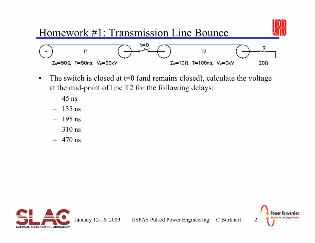
Homework #1: Transmission Line Bounce

• The switch is closed at t=0 (and remains closed), calculate the voltage at the mid-point of line T2 for the following delays:– 45 ns– 135 ns– 195 ns– 310 ns– 470 ns


Solution Approach• The traveling wave model for transmission line behavior, translates the

90 kV charge voltage on T1 to 2 recirculation 45 kV waves.• On closure of the switch, the wave incident on T2 will be partially

transmitted and partially reflected, replacing the existing wave with 2 new ones.

• When each new wave encounters an impedance discontinuity, some portion will be transmitted and the rest reflected, again, replacing the existing wave with 2 new ones.

• Waves transmitted to the resistive load are dissipated.• At any location and time, the voltage is the sum of the wave voltages.• Calculate transmission and reflection coefficients.• Track waves

– Tree structure (as done in class)– Bounce diagram (used in the TTU notes)


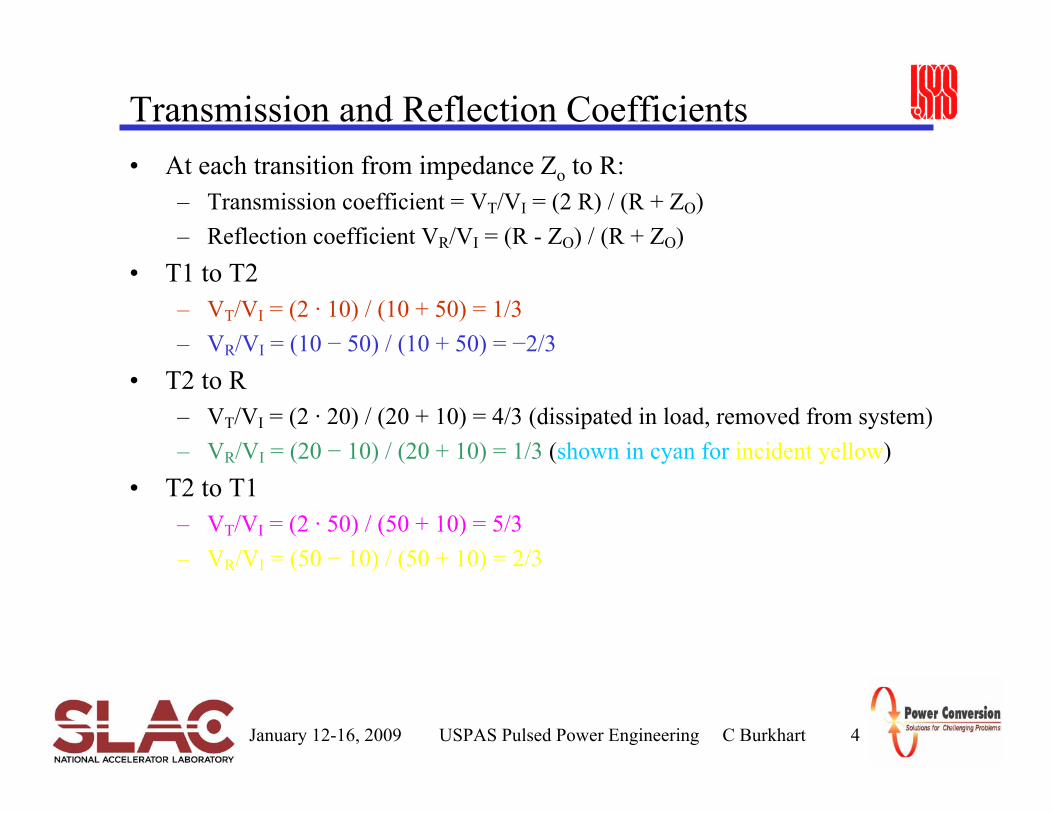
Transmission and Reflection Coefficients• At each transition from impedance Zo to R:

– Transmission coefficient = VT/VI = (2 R) / (R + ZO)– Reflection coefficient VR/VI = (R - ZO) / (R + ZO)

• T1 to T2– VT/VI = (2 · 10) / (10 + 50) = 1/3– VR/VI = (10 − 50) / (10 + 50) = −2/3

• T2 to R– VT/VI = (2 · 20) / (20 + 10) = 4/3 (dissipated in load, removed from system)– VR/VI = (20 − 10) / (20 + 10) = 1/3 (shown in cyan for incident yellow)

• T2 to T1– VT/VI = (2 · 50) / (50 + 10) = 5/3– VR/VI = (50 − 10) / (50 + 10) = 2/3


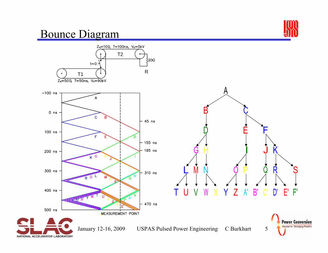
Bounce Diagram

T1

T2

R


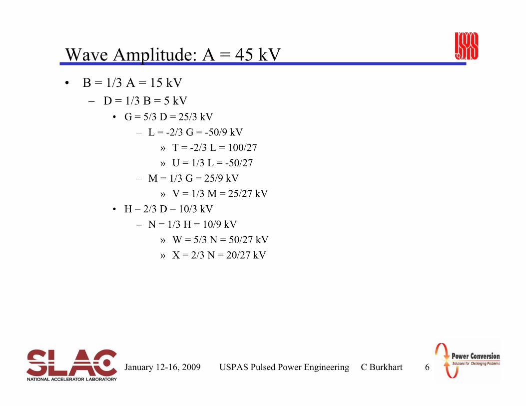
Wave Amplitude: A = 45 kV• B = 1/3 A = 15 kV

– D = 1/3 B = 5 kV• G = 5/3 D = 25/3 kV

– L = -2/3 G = -50/9 kV» T = -2/3 L = 100/27» U = 1/3 L = -50/27

– M = 1/3 G = 25/9 kV» V = 1/3 M = 25/27 kV

• H = 2/3 D = 10/3 kV– N = 1/3 H = 10/9 kV

» W = 5/3 N = 50/27 kV» X = 2/3 N = 20/27 kV


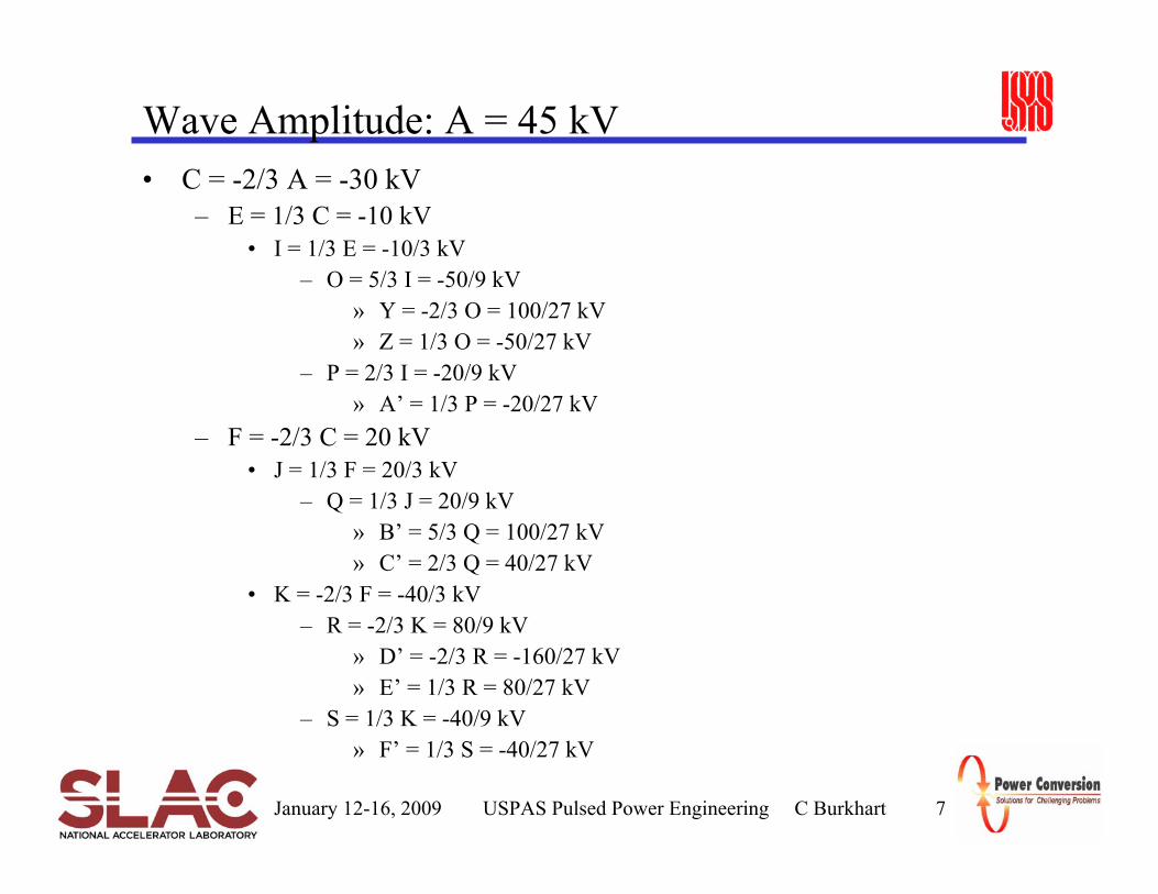
Wave Amplitude: A = 45 kV• C = -2/3 A = -30 kV

– E = 1/3 C = -10 kV• I = 1/3 E = -10/3 kV

– O = 5/3 I = -50/9 kV» Y = -2/3 O = 100/27 kV» Z = 1/3 O = -50/27 kV

– P = 2/3 I = -20/9 kV» A’ = 1/3 P = -20/27 kV

– F = -2/3 C = 20 kV• J = 1/3 F = 20/3 kV

– Q = 1/3 J = 20/9 kV» B’ = 5/3 Q = 100/27 kV» C’ = 2/3 Q = 40/27 kV

• K = -2/3 F = -40/3 kV– R = -2/3 K = 80/9 kV

» D’ = -2/3 R = -160/27 kV» E’ = 1/3 R = 80/27 kV

– S = 1/3 K = -40/9 kV» F’ = 1/3 S = -40/27 kV


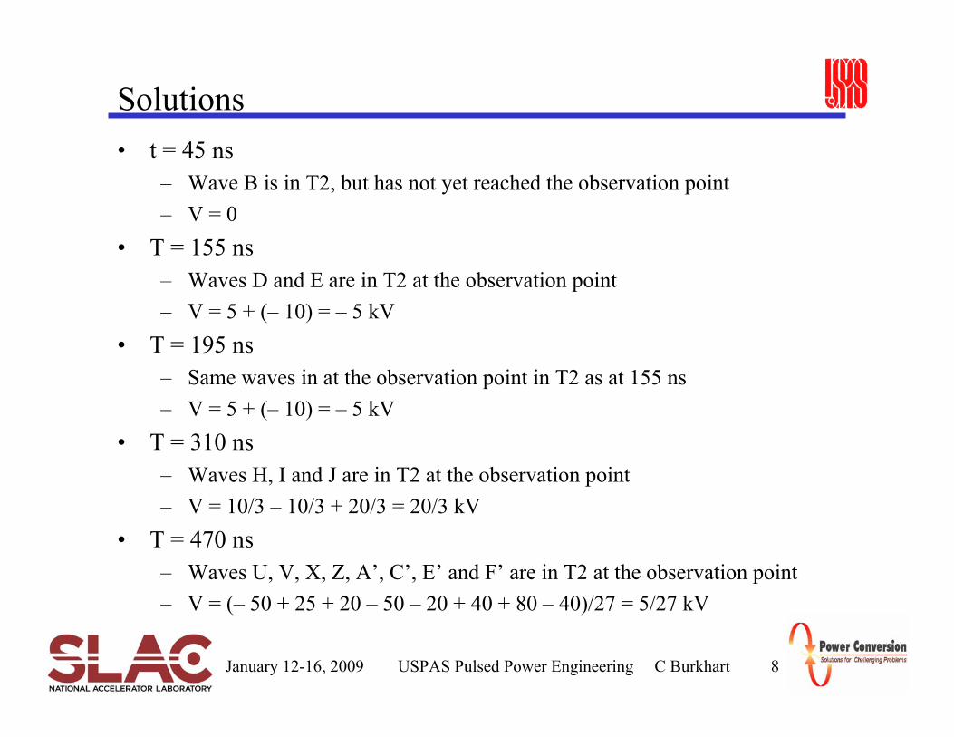
Solutions• t = 45 ns

– Wave B is in T2, but has not yet reached the observation point– V = 0

• T = 155 ns– Waves D and E are in T2 at the observation point– V = 5 + (– 10) = – 5 kV

• T = 195 ns– Same waves in at the observation point in T2 as at 155 ns– V = 5 + (– 10) = – 5 kV

• T = 310 ns– Waves H, I and J are in T2 at the observation point– V = 10/3 – 10/3 + 20/3 = 20/3 kV

• T = 470 ns– Waves U, V, X, Z, A’, C’, E’ and F’ are in T2 at the observation point– V = (– 50 + 25 + 20 – 50 – 20 + 40 + 80 – 40)/27 = 5/27 kV


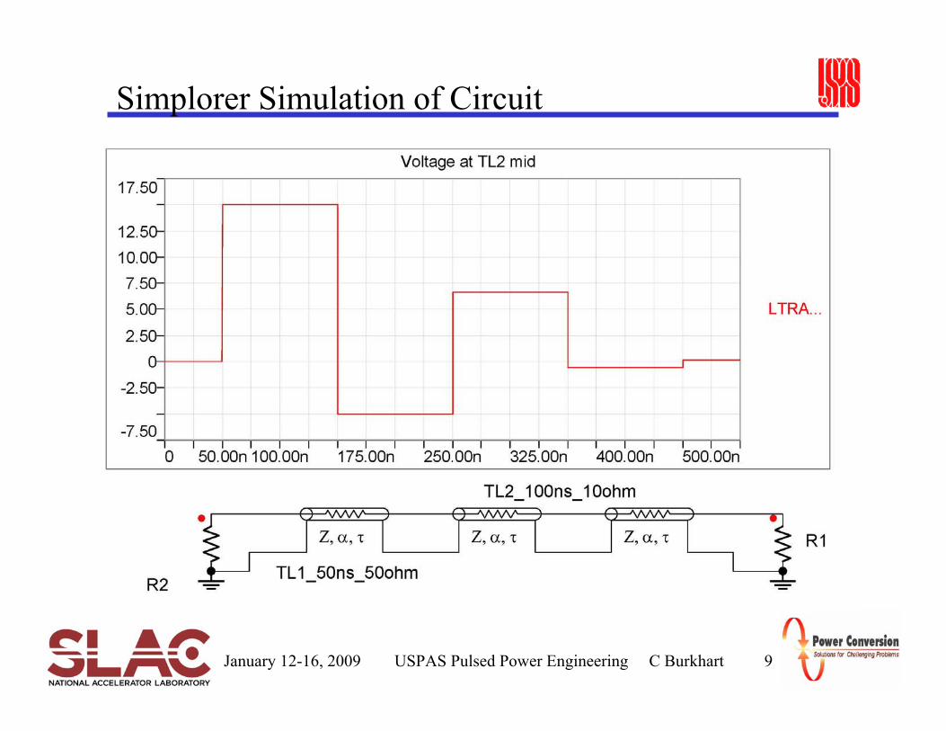
Simplorer Simulation of Circuit


Homework #2: Pulse Forming Network Design• Design a PFN to the following specifications:

– Impedance: Z = 10 Ω– Pulse duration: τ = 5 μs– Number of stages: N = 5– 50 kV charge voltage– We discussed several approaches for PFN design. For this exercise,

please use the “practical” implementation of the E-type Guillemin topology (page 51 of PPE Basic Topologies).

– Include a design for the inductor(s)


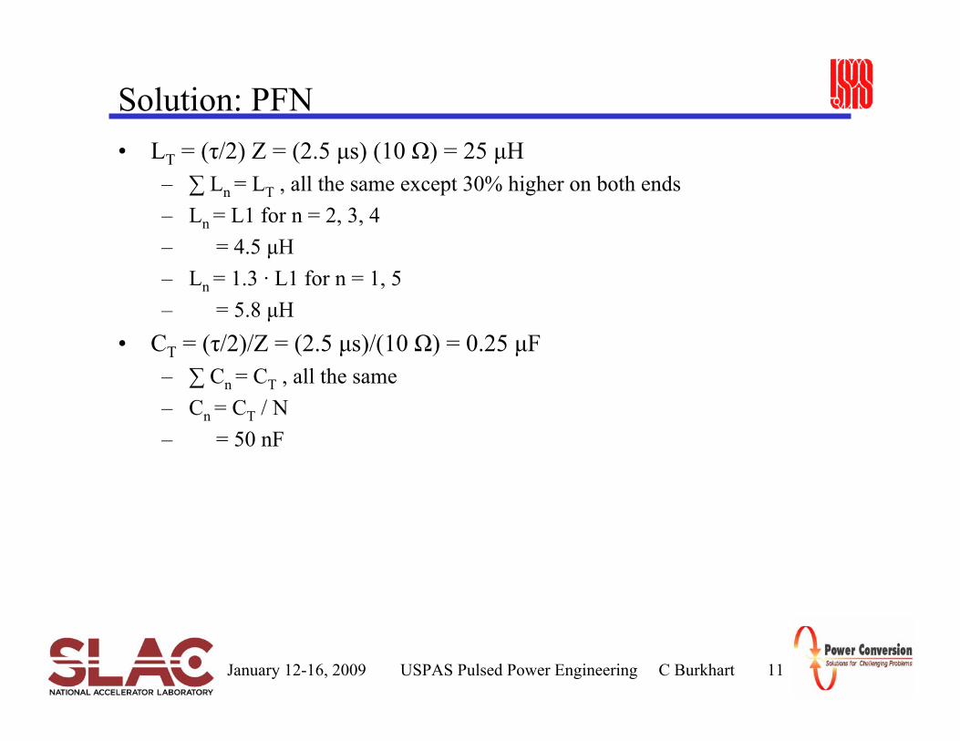
Solution: PFN• LT = (τ/2) Z = (2.5 μs) (10 Ω) = 25 μH

– ∑ Ln = LT , all the same except 30% higher on both ends– Ln = L1 for n = 2, 3, 4 – = 4.5 μH– Ln = 1.3 · L1 for n = 1, 5– = 5.8 μH

• CT = (τ/2)/Z = (2.5 μs)/(10 Ω) = 0.25 μF– ∑ Cn = CT , all the same– Cn = CT / N– = 50 nF


A Solution (E Pluribus Unum): Inductor• Design considerations

– High voltage: • Charge to 50 kV, avoid field enhancements that could arc or corona• Transient voltage as high as 50 kV across inductor, avoid turn-turn breakdown

– Current• Imatched = 2.5 kA

– Modest magnetic forces on coils• Average current

– Don’t know PRF, if we assume 100 Hz– <I> = 100 Hz · 5 μs · 2.5 kA = 1.25 A, therefore don’t need much copper– Skin depth, δ = (2.6 · τ ½) (ρ/ρc)½ = (2.6 · 5 μs½) (2.6/1.7)½ = 7 mm

[see page 4 of the “Materials” slides, above is simplified form for pulse length]• Size

– Want something that will “mate” to capacitors with short leads (stray L)– Caps will be similar to Maxwell 37612, except at 2X voltage (4X volume), so expect

caps to be ~4” X 6” X 10” long, so caps all side-by-side will be ~0.6 m, so that would be a good length for inductor

– Mutual inductance• Need ~15% mutual inductance between adjacent inductors E-type design• Can be achieved with a coil radius of 3 cm (for the rest of the final coil parameters)• Estimate the mutual inductance by calculating inductance for the length of a single coil (L = Ln)

then repeat calculation for a coil of twice the length (L = 2Ln + M), “extra” inductance is M


Coil design• L = N2μ π r2 /ℓ (will be a pretty good approximation, for a long coil)

25 μH = N2 · 1.26 X 10-6 · π · (3 X 10-2)2 / 0.6→N = 66 turns: 15 turns for coils 1 and 5, 12 turns for coils 2, 3 and 4

• Construction– Conductor: ¼” copper refrigeration tubing

• Flexible enough to wind• Rigid enough to be self-supporting• Large enough diameter to minimize electrical field enhancement

– Mandrel: 2-1/8” diameter heavy wall PVC tubing• Puts conductor centers at 3-cm-radius• Good mechanical material• Inexpensive


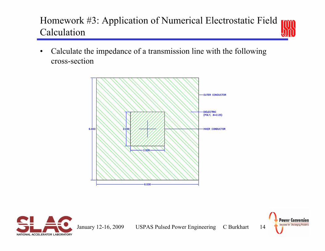
Homework #3: Application of Numerical Electrostatic Field Calculation

• Calculate the impedance of a transmission line with the following cross-section


Solution Technique• Transmission line impedance can be calculated from

– Z = τ/C, or= 1/[(C/ℓ) · v]• Where C/ℓ is capacitance per unit length • And v is the propagation velocity for EM energy in the transmission line• v = c/ε0.5

• Capacitance per unit length can be calculated from electric field energy per unit length (E/ℓ) and voltage difference between conductors (V)– C/ℓ = (2 · E/ℓ)/V2

• The electrostatic field solver can calculate the electric field energy


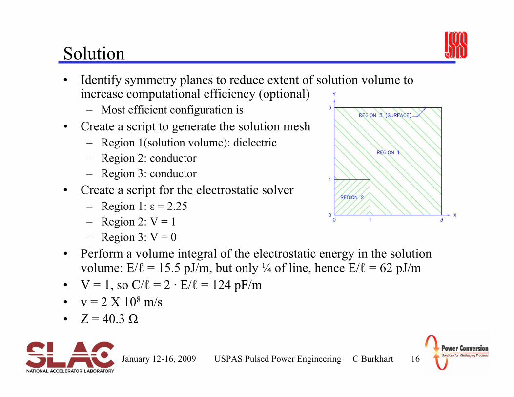
Solution• Identify symmetry planes to reduce extent of solution volume to

increase computational efficiency (optional)– Most efficient configuration is

• Create a script to generate the solution mesh– Region 1(solution volume): dielectric– Region 2: conductor– Region 3: conductor

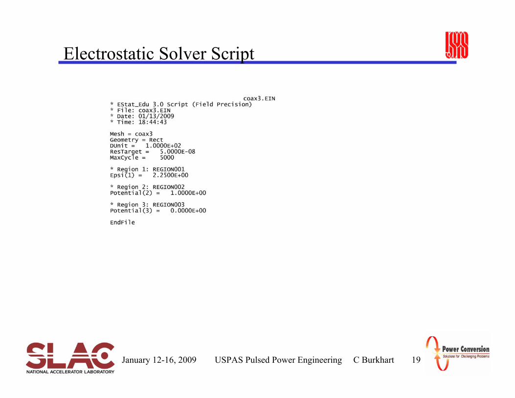
• Create a script for the electrostatic solver– Region 1: ε = 2.25– Region 2: V = 1– Region 3: V = 0

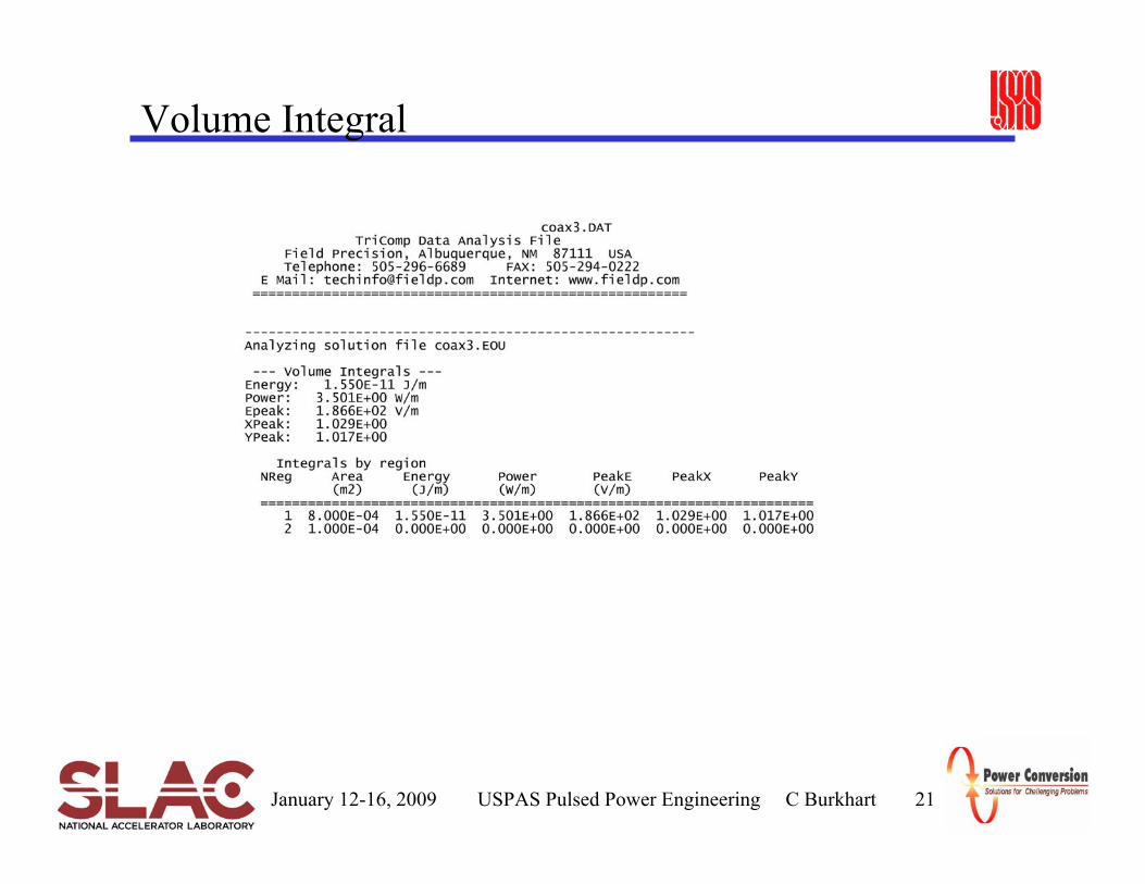
• Perform a volume integral of the electrostatic energy in the solution volume: E/ℓ = 15.5 pJ/m, but only ¼ of line, hence E/ℓ = 62 pJ/m

• V = 1, so C/ℓ = 2 · E/ℓ = 124 pF/m• v = 2 X 108 m/s• Z = 40.3 Ω


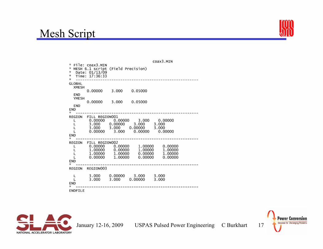
Mesh Script


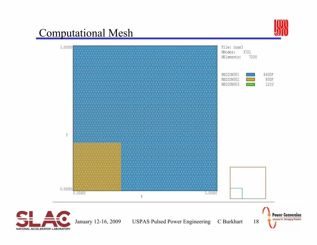
Computational Mesh

0.00000 3.00000X

0.00000

3.00000

Y

File: coax3NNodes: 3721NElements: 7200

REGION001 6400FREGION002 800FREGION003 121U


Electrostatic Solver Script


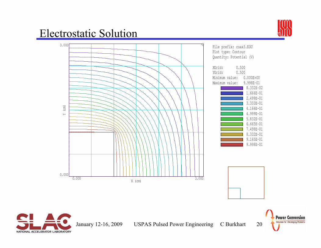
Electrostatic Solution

0.000 3.000X (cm)

0.000

3.000

Y (cm)

File prefix: coax3.EOUPlot type: ContourQuantity: Potential (V)

XGrid: 0.500YGrid: 0.500Minimum value: 0.000E+00Maximum value: 9.998E-01

8.332E-02 1.666E-01 2.499E-01 3.333E-01 4.166E-01 4.999E-01 5.832E-01 6.665E-01 7.498E-01 8.332E-01 9.165E-01 9.998E-01


Volume Integral


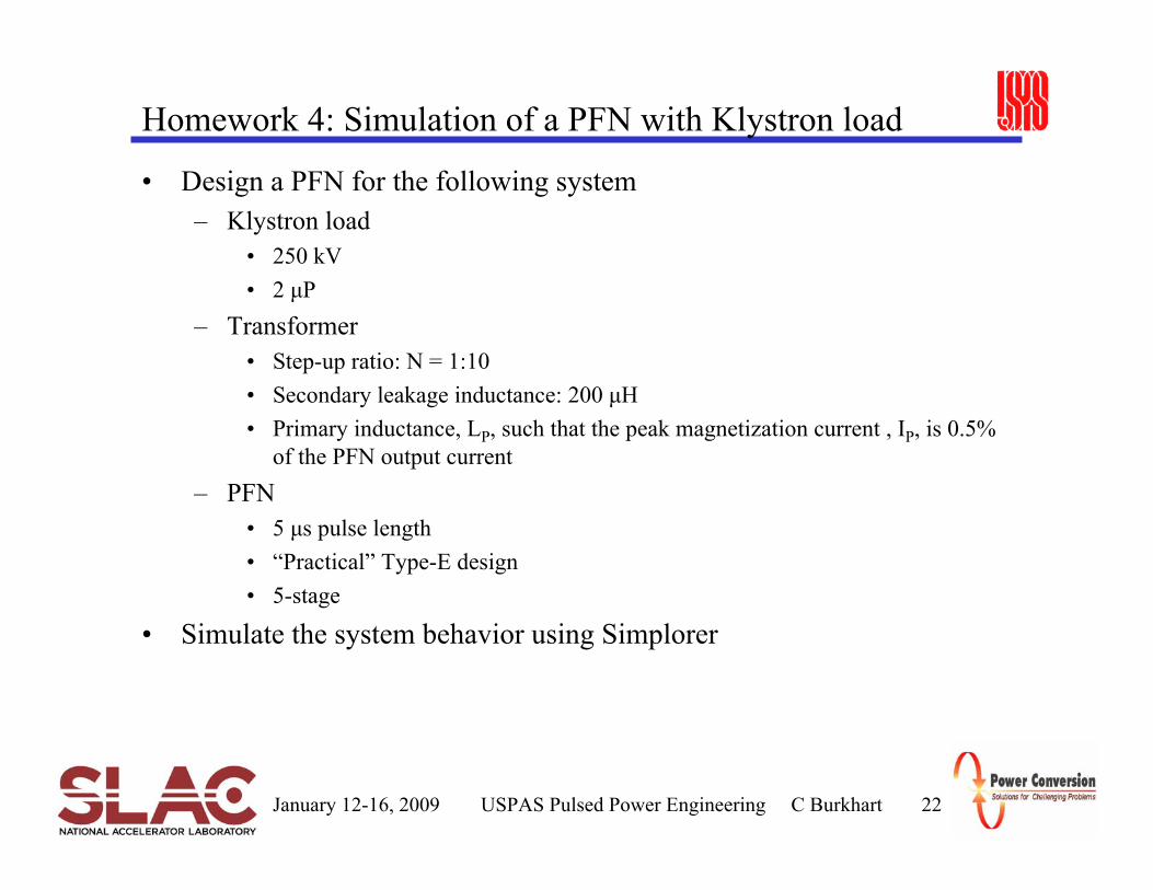
Homework 4: Simulation of a PFN with Klystron load

• Design a PFN for the following system– Klystron load

• 250 kV• 2 μP

– Transformer• Step-up ratio: N = 1:10 • Secondary leakage inductance: 200 μH• Primary inductance, LP, such that the peak magnetization current , IP, is 0.5%

of the PFN output current– PFN

• 5 μs pulse length• “Practical” Type-E design• 5-stage

• Simulate the system behavior using Simplorer


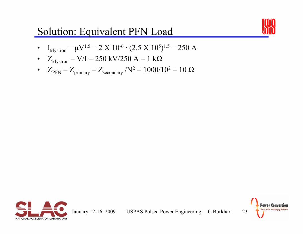
Solution: Equivalent PFN Load• Iklystron = μV1.5 = 2 X 10-6 · (2.5 X 105)1.5 = 250 A• Zklystron = V/I = 250 kV/250 A = 1 kΩ• ZPFN = Zprimary = Zsecondary /N2 = 1000/102 = 10 Ω


Solution: PFN• LT = (τ/2) Z = (2.5 μs) (10 Ω) = 25 μH

– ∑ Ln = LT , all the same except 30% higher on both ends– Ln = L1 for n = 2, 3, 4 – = 4.5 μH– Ln = 1.3 · L1 for n = 1, 5– = 5.8 μH

• CT = (τ/2)/Z = (2.5 μs)/(10 Ω) = 0.25 μF– ∑ Cn = CT , all the same– Cn = CT / N– = 50 nF


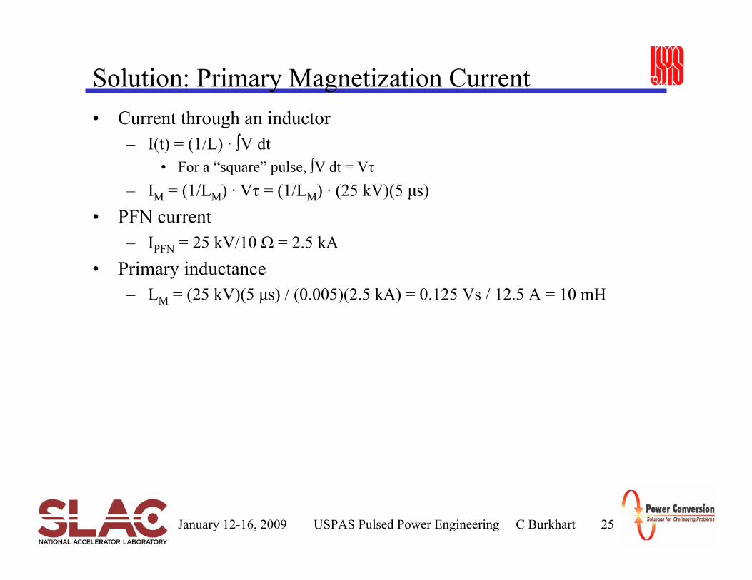
Solution: Primary Magnetization Current• Current through an inductor

– I(t) = (1/L) · ∫V dt• For a “square” pulse, ∫V dt = Vτ

– IM = (1/LM) · Vτ = (1/LM) · (25 kV)(5 μs)• PFN current

– IPFN = 25 kV/10 Ω = 2.5 kA• Primary inductance

– LM = (25 kV)(5 μs) / (0.005)(2.5 kA) = 0.125 Vs / 12.5 A = 10 mH


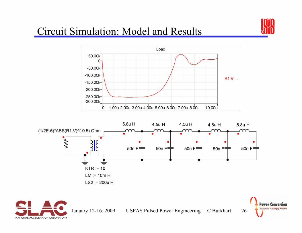
Circuit Simulation: Model and Results


Final Exam1) Calculate the perveance of a 500 kV, 250 A klystron

μ = I / V1.5

= 250 / (5 X 105)1.5

= 0.707 μP2) Calculate the inductance of 1 m of 50 Ω poly dielectric (εr = 2.25) coax

L = τ · Z τ = ℓ/v

v = c/ε0.5

= 3 X 108/2.250.5

= 2 X 108 m/s= 1 m / 2 X 108 m/s= 5 ns

= 5 ns · 50 Ω= 0.25 μH


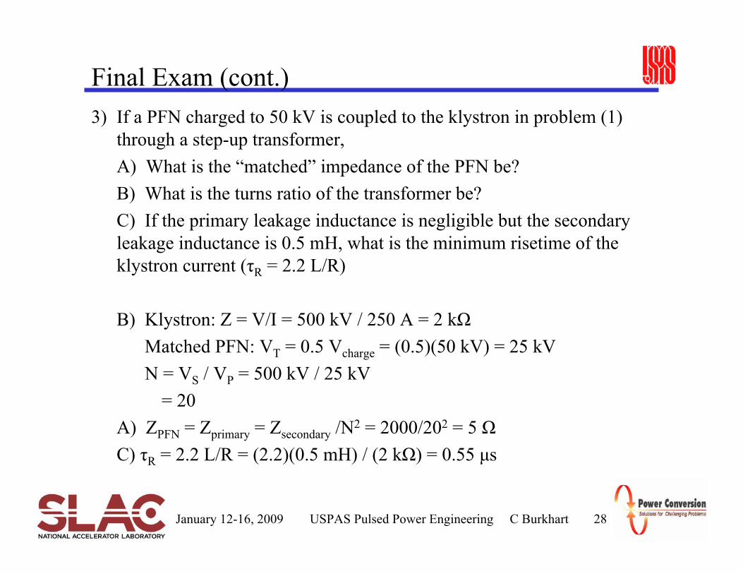
Final Exam (cont.)3) If a PFN charged to 50 kV is coupled to the klystron in problem (1)

through a step-up transformer,A) What is the “matched” impedance of the PFN be?B) What is the turns ratio of the transformer be?C) If the primary leakage inductance is negligible but the secondary leakage inductance is 0.5 mH, what is the minimum risetime of the klystron current (τR = 2.2 L/R)

B) Klystron: Z = V/I = 500 kV / 250 A = 2 kΩMatched PFN: VT = 0.5 Vcharge = (0.5)(50 kV) = 25 kVN = VS / VP = 500 kV / 25 kV

= 20A) ZPFN = Zprimary = Zsecondary /N2 = 2000/202 = 5 ΩC) τR = 2.2 L/R = (2.2)(0.5 mH) / (2 kΩ) = 0.55 μs


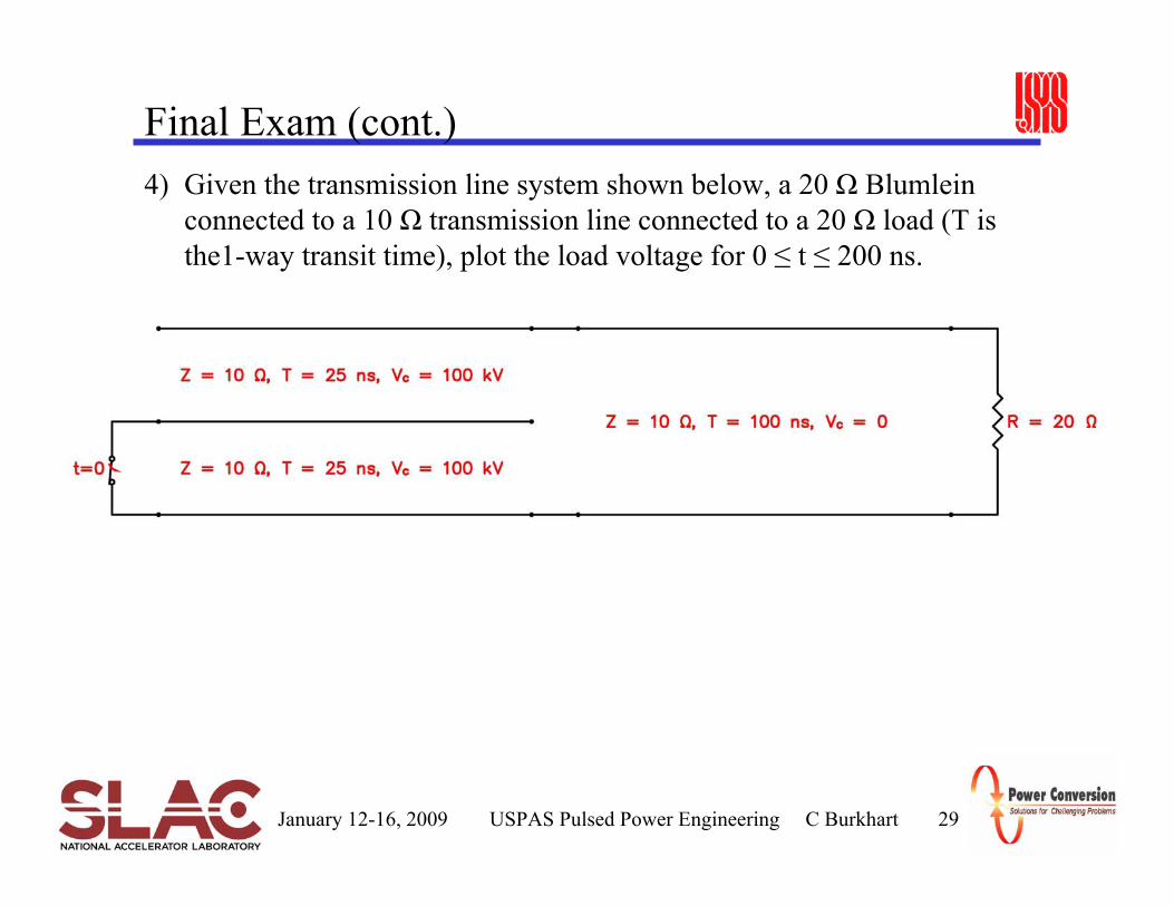
Final Exam (cont.)4) Given the transmission line system shown below, a 20 Ω Blumlein

connected to a 10 Ω transmission line connected to a 20 Ω load (T is the1-way transit time), plot the load voltage for 0 ≤ t ≤ 200 ns.


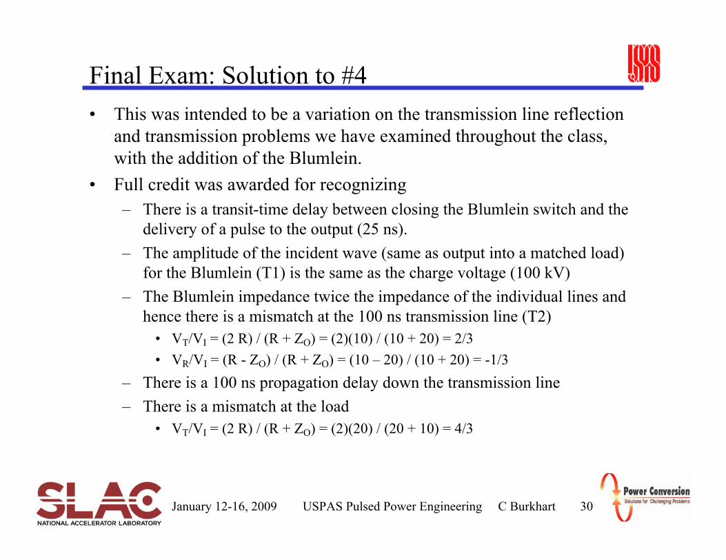
Final Exam: Solution to #4• This was intended to be a variation on the transmission line reflection

and transmission problems we have examined throughout the class,with the addition of the Blumlein.

• Full credit was awarded for recognizing– There is a transit-time delay between closing the Blumlein switch and the

delivery of a pulse to the output (25 ns).– The amplitude of the incident wave (same as output into a matched load)

for the Blumlein (T1) is the same as the charge voltage (100 kV)– The Blumlein impedance twice the impedance of the individual lines and

hence there is a mismatch at the 100 ns transmission line (T2)• VT/VI = (2 R) / (R + ZO) = (2)(10) / (10 + 20) = 2/3• VR/VI = (R - ZO) / (R + ZO) = (10 – 20) / (10 + 20) = -1/3

– There is a 100 ns propagation delay down the transmission line– There is a mismatch at the load

• VT/VI = (2 R) / (R + ZO) = (2)(20) / (20 + 10) = 4/3


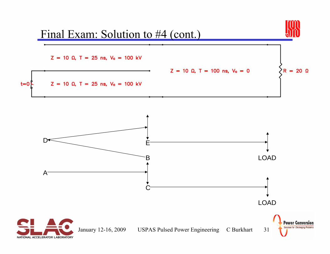
Final Exam: Solution to #4 (cont.)

A

B

C

ED

LOAD

LOAD


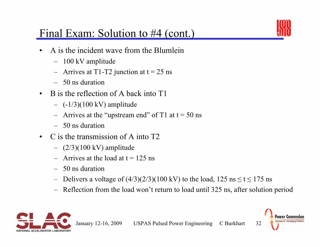
Final Exam: Solution to #4 (cont.)• A is the incident wave from the Blumlein

– 100 kV amplitude– Arrives at T1-T2 junction at t = 25 ns– 50 ns duration

• B is the reflection of A back into T1– (-1/3)(100 kV) amplitude– Arrives at the “upstream end” of T1 at t = 50 ns– 50 ns duration

• C is the transmission of A into T2– (2/3)(100 kV) amplitude– Arrives at the load at t = 125 ns– 50 ns duration– Delivers a voltage of (4/3)(2/3)(100 kV) to the load, 125 ns ≤ t ≤ 175 ns– Reflection from the load won’t return to load until 325 ns, after solution period


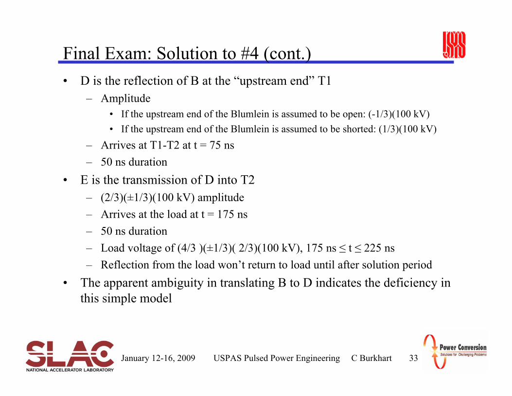
Final Exam: Solution to #4 (cont.)• D is the reflection of B at the “upstream end” T1

– Amplitude• If the upstream end of the Blumlein is assumed to be open: (-1/3)(100 kV) • If the upstream end of the Blumlein is assumed to be shorted: (1/3)(100 kV)

– Arrives at T1-T2 at t = 75 ns– 50 ns duration

• E is the transmission of D into T2– (2/3)(±1/3)(100 kV) amplitude– Arrives at the load at t = 175 ns– 50 ns duration– Load voltage of (4/3 )(±1/3)( 2/3)(100 kV), 175 ns ≤ t ≤ 225 ns– Reflection from the load won’t return to load until after solution period

• The apparent ambiguity in translating B to D indicates the deficiency in this simple model


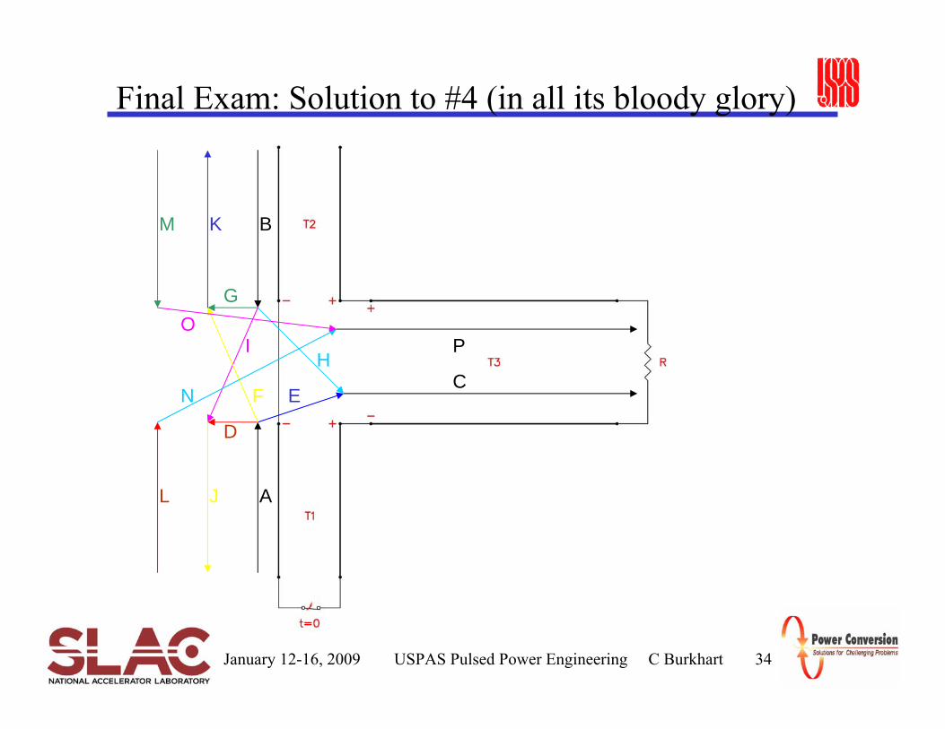
Final Exam: Solution to #4 (in all its bloody glory)

A

EC

F

B

HI

D

G

P

J

K

L

M

N

O


Final Exam: #4 Transmission & Reflection– T1

• VT/VI = (2 R) / (R + ZO) = (2)(10 +10) / (10 + 10 + 10) = 4/3– VT/VI (T2) = (1/2) VT/VI = 2/3– VT/VI (T3) = (-1/2) VT/VI = -2/3 (“sense” of 2 lines reversed)

• VR/VI = (R - ZO) / (R + ZO) = (10 +10 – 10) / (10 + 10 + 10) = 1/3– T2

• VT/VI = (2)(10 +10) / (10 + 10 + 10) = 4/3– VT/VI (T3) = (1/2) VT/VI = 2/3– VT/VI (T1) = (1/2) VT/VI = 2/3

• VR/VI = (10 +10 – 10) / (10 + 10 + 10) = 1/3– T3

• VT/VI = (2)(10 +10) / (10 + 10 + 10) = 4/3– VT/VI (T1) = (-1/2) VT/VI = -2/3– VT/VI (T2) = (1/2) VT/VI = 2/3

• VR/VI = (10 +10 – 10) / (10 + 10 + 10) = 1/3– Load: as before


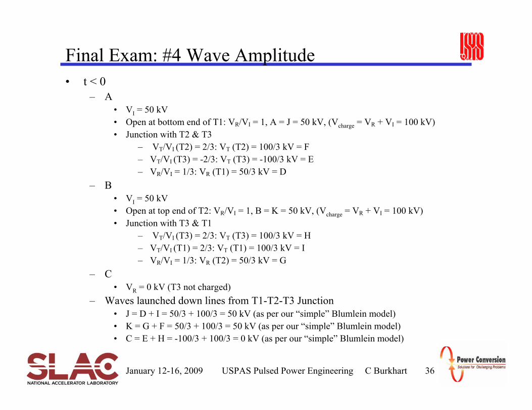
Final Exam: #4 Wave Amplitude• t < 0

– A• VI = 50 kV• Open at bottom end of T1: VR/VI = 1, A = J = 50 kV, (Vcharge = VR + VI = 100 kV)• Junction with T2 & T3

– VT/VI (T2) = 2/3: VT (T2) = 100/3 kV = F– VT/VI (T3) = -2/3: VT (T3) = -100/3 kV = E– VR/VI = 1/3: VR (T1) = 50/3 kV = D

– B• VI = 50 kV• Open at top end of T2: VR/VI = 1, B = K = 50 kV, (Vcharge = VR + VI = 100 kV)• Junction with T3 & T1

– VT/VI (T3) = 2/3: VT (T3) = 100/3 kV = H– VT/VI (T1) = 2/3: VT (T1) = 100/3 kV = I– VR/VI = 1/3: VR (T2) = 50/3 kV = G

– C• VR = 0 kV (T3 not charged)

– Waves launched down lines from T1-T2-T3 Junction• J = D + I = 50/3 + 100/3 = 50 kV (as per our “simple” Blumlein model)• K = G + F = 50/3 + 100/3 = 50 kV (as per our “simple” Blumlein model)• C = E + H = -100/3 + 100/3 = 0 kV (as per our “simple” Blumlein model)


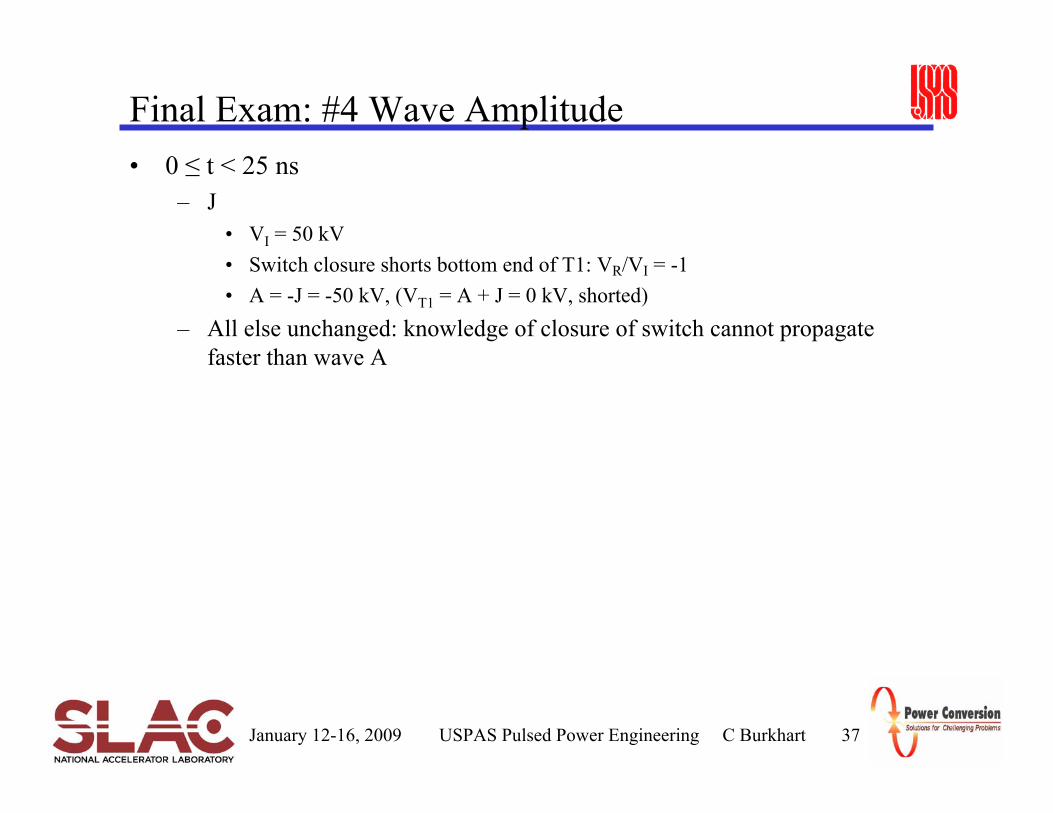
Final Exam: #4 Wave Amplitude• 0 ≤ t < 25 ns

– J• VI = 50 kV• Switch closure shorts bottom end of T1: VR/VI = -1 • A = -J = -50 kV, (VT1 = A + J = 0 kV, shorted)

– All else unchanged: knowledge of closure of switch cannot propagate faster than wave A


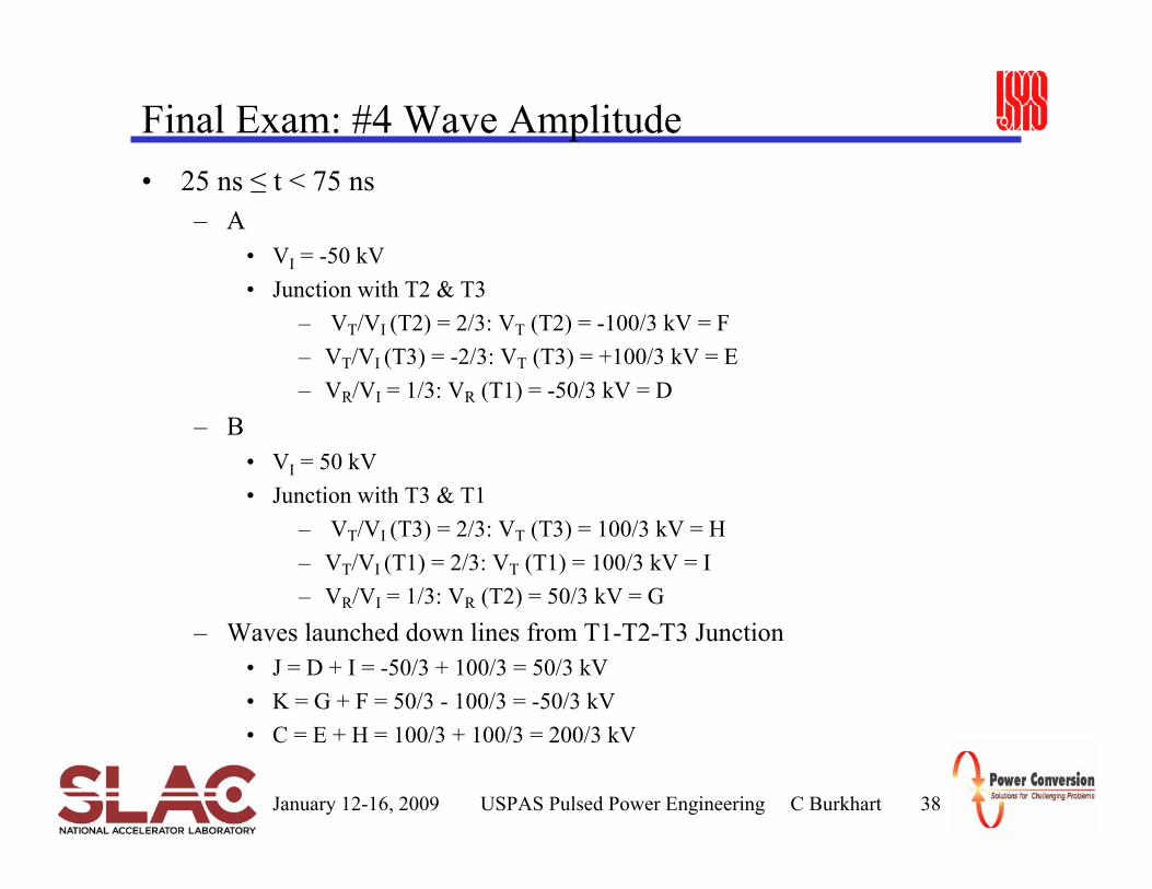
Final Exam: #4 Wave Amplitude• 25 ns ≤ t < 75 ns

– A• VI = -50 kV• Junction with T2 & T3

– VT/VI (T2) = 2/3: VT (T2) = -100/3 kV = F– VT/VI (T3) = -2/3: VT (T3) = +100/3 kV = E– VR/VI = 1/3: VR (T1) = -50/3 kV = D

– B• VI = 50 kV• Junction with T3 & T1

– VT/VI (T3) = 2/3: VT (T3) = 100/3 kV = H– VT/VI (T1) = 2/3: VT (T1) = 100/3 kV = I– VR/VI = 1/3: VR (T2) = 50/3 kV = G

– Waves launched down lines from T1-T2-T3 Junction• J = D + I = -50/3 + 100/3 = 50/3 kV• K = G + F = 50/3 - 100/3 = -50/3 kV• C = E + H = 100/3 + 100/3 = 200/3 kV


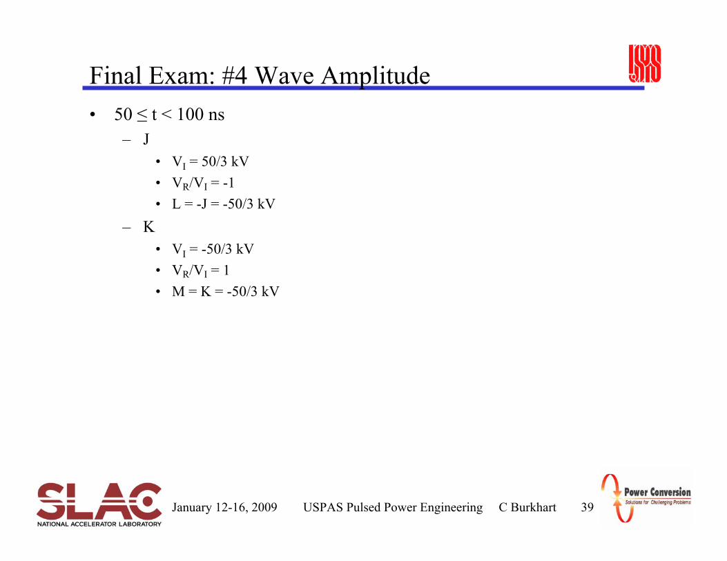
Final Exam: #4 Wave Amplitude• 50 ≤ t < 100 ns

– J• VI = 50/3 kV• VR/VI = -1 • L = -J = -50/3 kV

– K• VI = -50/3 kV• VR/VI = 1 • M = K = -50/3 kV


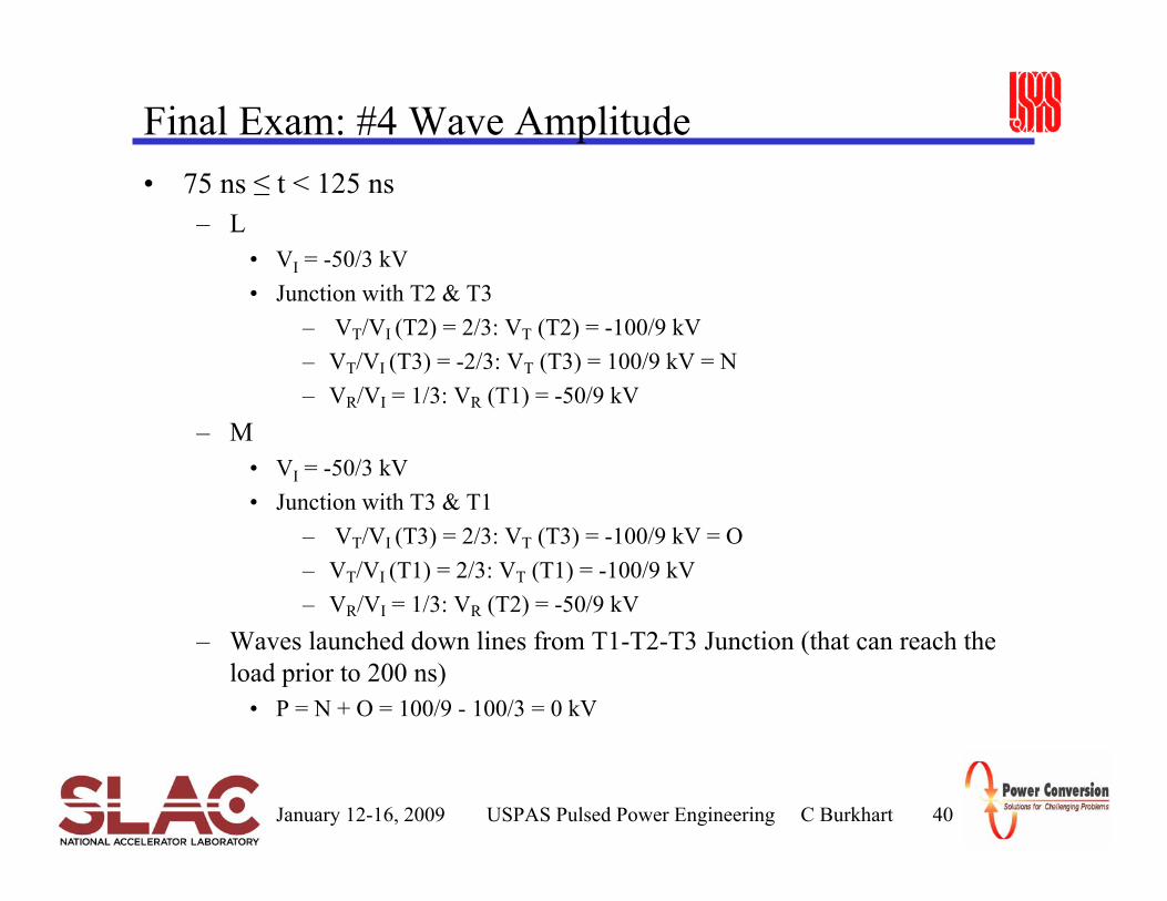
Final Exam: #4 Wave Amplitude• 75 ns ≤ t < 125 ns

– L• VI = -50/3 kV• Junction with T2 & T3

– VT/VI (T2) = 2/3: VT (T2) = -100/9 kV – VT/VI (T3) = -2/3: VT (T3) = 100/9 kV = N– VR/VI = 1/3: VR (T1) = -50/9 kV

– M• VI = -50/3 kV• Junction with T3 & T1

– VT/VI (T3) = 2/3: VT (T3) = -100/9 kV = O– VT/VI (T1) = 2/3: VT (T1) = -100/9 kV– VR/VI = 1/3: VR (T2) = -50/9 kV

– Waves launched down lines from T1-T2-T3 Junction (that can reach the load prior to 200 ns)

• P = N + O = 100/9 - 100/3 = 0 kV


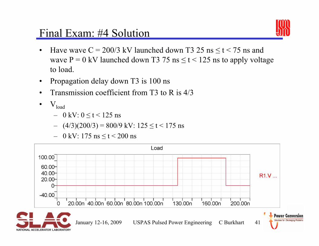
Final Exam: #4 Solution• Have wave C = 200/3 kV launched down T3 25 ns ≤ t < 75 ns and

wave P = 0 kV launched down T3 75 ns ≤ t < 125 ns to apply voltage to load.

• Propagation delay down T3 is 100 ns• Transmission coefficient from T3 to R is 4/3• Vload

– 0 kV: 0 ≤ t < 125 ns– (4/3)(200/3) = 800/9 kV: 125 ≤ t < 175 ns– 0 kV: 175 ns ≤ t < 200 ns


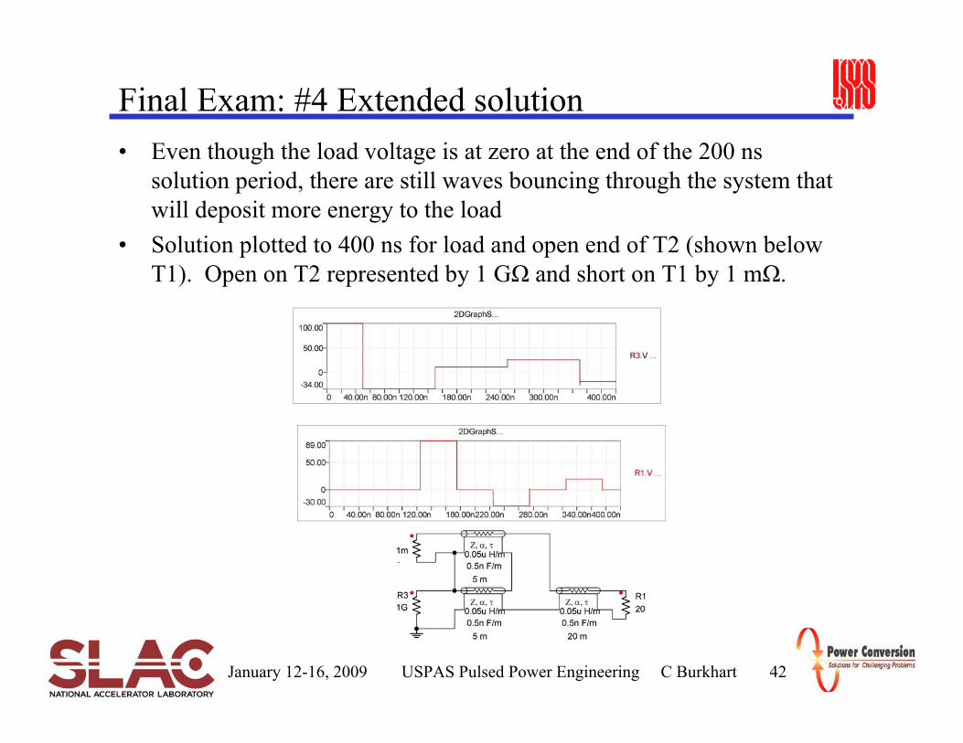
Final Exam: #4 Extended solution• Even though the load voltage is at zero at the end of the 200 ns

solution period, there are still waves bouncing through the system that will deposit more energy to the load

• Solution plotted to 400 ns for load and open end of T2 (shown below T1). Open on T2 represented by 1 GΩ and short on T1 by 1 mΩ.

Documents

PPE Homework Solution Set - USPASuspas.fnal.gov/materials/09VU/PPE_HomeworkSolution.pdf · Pulsed Power Engineering Homework Solution Set January 12-16, 2009 Craig Burkhart, PhD Power