Embed Size (px)
Citation preview

Prediction of forced convection heat transfer toLead-Bismuth-Eutectic
ROMAN THIELE
Licentiate ThesisStockholm, Sweden, 2013

TRITA-FYS 2013:19ISSN 0280-316XISRN KTH/FYS/--13:19—SEISBN 978-91-7501-784-6
AlbaNovaRoslagstullsbacken 21
10691 StockholmSweden
Akademisk avhandling som med tillstånd av Kungl Tekniska högskolan framläggestill offentlig granskning för avläggande av teknologie licentiatexamen i reaktortek-nologie måndagen den 10 juni, 2013 kl 10:00 i FA32, AlbaNova, Stockholm.
c© Roman Thiele, June 2013
Tryck: Universitetsservice US AB
Doktorsavhandlingssammanfattning
Metallkylda reaktorer har framförts som ett av ett flertal alternativ för framtidensGeneration-IV system. Dessa reaktorer möjliggör för en mer hållbar och säker ener-giproduktion från kärnkraft. Ett av målen för nästa generations kärnkraft är attde ska vara hållbara ur resursperspektiv och kunna återvinna sitt eget bränsle. Itillägg måste dessa system vara ekonomiskt hållbara, antingen billigare eller jäm-förbara i kostnad med dagens system. Ett annat krav för framtidens reaktorer attde håller en högre säkerhetsstandard, både under olycksförhållanden men även förförhindrande av otillåten spridning av känsligt material. Metallkylda reaktorer ärett möjligt alternativ som kan uppfylla dessa krav.
Arbetet som presenteras här är fokuserat på termohydraulik i metallkylda re-aktorer. Värmeöverföring i metallkylda reaktorer fungerar annorlunda än i dagensreaktorer som använder vatten som kylmedel. Detta medför att verktyg och dator-modeller som har utvecklats för termohydraulik i vattenkylda system måste va-lideras innan de kan användas i utvecklingsprocessen för den nya generationensreaktorer.
Konvektiv värmeöverföring är beroende av kylmedlets flödesregim. Flödesregi-merna är forcerad, blandad och naturlig konvektion. Tidigare forskning har visat attvärmeöverföring under blandad och naturlig konvektion inte kan modelleras medförsta ordningens RANS (Reynolds Averaged) modeller utan att först modifieraRANS-modellens temperatur och energi-ekvationer.
Konventionell RANS-modellering använder sig av den så kallade “Reynolds ana-logy” metoden vilket betyder ett konstant Prandtl-värde under turbulent flöde. Det-ta möjliggör modellerandet av turbulent värmeflöde med begränsade beräkningsre-surser. Det är dock inte möjligt att använda denna approximation under blandadeller naturligt konvektiv värmeöverföring i kylmedel med lågt Prandtl-värde såsombly och bly-vismut.
Den numeriska beräkningen använder sig av RANS-modellen med Boussinesq’sapproximation för flytkraft och konstanta fysiska egenskaper för vätskan beräknadevid en referenstemperatur. Beräkningsmodellen använder Reynolds medeltemperatur-ekvation med ett turbulent Prandtl-värde.
Dessa beräkningar har jämförts med publicerad experimentell data. Mätdatakommer från TALL-anläggningen i Stockholm och från THESYS2-anläggningen iKarlsruhe, Tyskland. Båda databiblioteken innehåller temperaturmätningar under
iii
iv
forcerat konvektiv flöde av bly-vismut i ett ihåligt rör. Värdena från THESYS2innehåller även hastighetsmätningar. Ett konstant värmeflöde applicerades på deninre väggen av röret och förhållandet vid den yttre väggen är adiabatiskt.
Dessa experiment har modellerats i OpenFOAM och CFX. I OpenFOAM an-vänds ett quasi 2D-mesh. I CFX användes ett 3D-mesh efter att det stod klart atten quasi 2D-modell inte gav acceptabla resultat. En sensitivitetsanalys av resulta-ten utfördes för att visa på känsligheten av olika indata i modellen. Den viktigasteparametern i indatat visade sig vara det turbulenta Prandtl-värdet. Resultaten avtre olika turbulensmodeller, low-Re k-ε, q-ζ och k-ω-SST, jämfördes med varandraoch med testdatat.
Resultaten från TALL-anläggningen användes enbart för en första utvärderingav turbulensmodellerna. Majoriteten av resultaten är baserade på jämförelser meddata från THESYS2. k-ε och q-ζ modellerna i OpenFOAM gav liknande resultat.Resultaten visar en god matchning av mätdata för hastighetsprofilen. Även tempe-raturberäkningarna gav acceptabla resultat med en avvikelse på 10%.
k-ω-SST-modellen har brister i hastighetsberäkningar men ger acceptabla re-sultat för temperaturprofilsberäkningar. Avvikelsen i väggtemperatursberäkningenär med 14% dock större än för de andra två modellerna. Eftersom hastighetsberäk-ningen har stora brister bör resultaten för temperaturberäkningen användas medstor försiktighet.
2D-resultaten i CFX ger stora avvikelser både i hastighet och temperaturpro-filsberäkningar. k-ω-SST-modellen i 3D ger acceptabla resultat i CFX, men beräk-ningsbördan för denna modell är orimligt tung.
Sensitivitetsanalysen har utförts enbart med resultaten från beräkningar i Open-FOAM. Bättre resultat bör kunna uppnås med en bättre gissning av Prandtl-värdet.I en beräkning sattes Prandtl-värdet till 1.96, baserat på en korrelation av Lyonsom modifierats av Cheng et. al..
Detta resulterade i en stor överskattning av väggtemperaturen och stora av-vikelser från experimentell data för temperaturprofilen. Ändring av indata såsomPrandtl-värde eller andra indata kopplade till värmeöverföring har ingen inverkanpå hastighetsprofilen.
Värden nära referensvärdet för Prandtl-värdet ger bäst resultat. Resultaten ärgenerellt väldigt känsliga för variationer av det turbulenta Prandtl-värdet. k-ω-SST-modellen är den känsligaste av de tre modeller som testats.
Denna studie har visat att användbara resultat för konvektiv värmeöverföringunder forcerat flöde för vätskor med lågt Prandtl-värde kan uppnås med första ord-ningens turbulens-modeller med användning av RANS-ekvationerna och “Reynoldsanalogy”-principen. Resultaten är känsliga för valet av turbulent Prandtl-värde.Det turbulenta Prandtl-värdet måste väljas noggrant och med hänsyn till vilkenturbulensmodell som används. Metoder som har utvecklats för en kod kan intedirekt appliceras i andra koder utan lämpliga modifikationer.
Abstract
The goal of this work is to investigate the capabilities of two different commercialcodes, OpenFOAM and ANSYS CFX, to predict forced convection heat transferin low Prandtl number fluids and investigate the sensitivity of these predictions tothe type of code and to several input parameters.
The goal of the work is accomplished by predicting forced convection heat trans-fer in two different experimental setups with the codes OpenFOAM and ANSYSCFX using three different turbulence models and varying the input parameters inan extensive sensitivity analysis. The computational results are compared two theexperimental data and analyzed for qualitative and quantitative parameters, suchas shape of velocity and temperature profiles, thickness of the boundary layers andwall temperatures.
The results show that predictions of the temperature and velocity field aregenerally sufficient to good, however, the sensitivity especially to the turbulentPrandtl number has to be taken into account when computing forced convectionheat transfer in low Prandtl number fluids. The results also show that methodsapplied to OpenFOAM cannot directly be applied to ANSYS CFX.
Keywords: Lead-bismuth-eutectic, Forced convective heat transfer, Turbulence-modeling, GEN-IV reactors
v


Acknowledgements
I would like to extend my gratitude to my fellow colleagues, who were good listenersand sometimes a source of inspiration during the course of this work. I would liketo thank Janne Wallenius for setting up the project, GENIUS, through which thiswork was possible and Henryk Anglart for providing me with the opportunity towork on this project.
A special thanks goes to Dr. Staffan Qvist halfway around the globe for a lastminute translation of the “Svensk sammanfattning” (Swedish summary).
I acknowledge the financial support by Vetenskapsrådet (Swedish ResearchCouncil), through the GENIUS project.
vii

Contents
Contents ix
List of Figures xi
List of Tables xv
1 Introduction 11.1 Research objective . . . . . . . . . . . . . . . . . . . . . . . . . . . . 2
2 Theoretical Background 32.1 Liquid metal cooled reactors . . . . . . . . . . . . . . . . . . . . . . . 32.2 Properties of low Prandtl number fluids . . . . . . . . . . . . . . . . 42.3 Flow regimes . . . . . . . . . . . . . . . . . . . . . . . . . . . . . . . 5
2.3.1 Turbulent Prandtl number concept . . . . . . . . . . . . . . . 62.4 Turbulence models . . . . . . . . . . . . . . . . . . . . . . . . . . . . 7
2.4.1 Launder-Sharma low Reynolds k-epsilon model . . . . . . . . 72.4.2 Menter k-omega-SST model . . . . . . . . . . . . . . . . . . . 82.4.3 Gibson-Daffa’Alla q-zeta model . . . . . . . . . . . . . . . . . 9
2.5 CFD modeling of heat transfer . . . . . . . . . . . . . . . . . . . . . 9
3 Methodology and Modeling 133.1 Governing equations . . . . . . . . . . . . . . . . . . . . . . . . . . . 133.2 Experimental data . . . . . . . . . . . . . . . . . . . . . . . . . . . . 143.3 Mesh and boundary conditions . . . . . . . . . . . . . . . . . . . . . 16
3.3.1 3D approach for CFX . . . . . . . . . . . . . . . . . . . . . . 193.4 Sensitivity analysis . . . . . . . . . . . . . . . . . . . . . . . . . . . . 193.5 Evaluation of the predictions . . . . . . . . . . . . . . . . . . . . . . 20
4 Discussion of Results 214.1 Computational results of the reference cases with OpenFOAM . . . 214.2 Computational results of the reference cases with ANSYS CFX . . . 234.3 Results of the sensitivity analysis . . . . . . . . . . . . . . . . . . . . 304.4 Code comparison . . . . . . . . . . . . . . . . . . . . . . . . . . . . . 39
ix

x CONTENTS
5 Conclusions and Future Work 41
Bibliography 43
List of Figures
2.1 Schematic of one of the envisioned designs for liquid metal fast reactorscooled with lead or LBE, (DOE, 2002) . . . . . . . . . . . . . . . . . . . 4
2.2 Scale difference and similarity of the thermal and momentum field influids with different molecular Prandtl numbers (LBE Handbook, 2007) 5
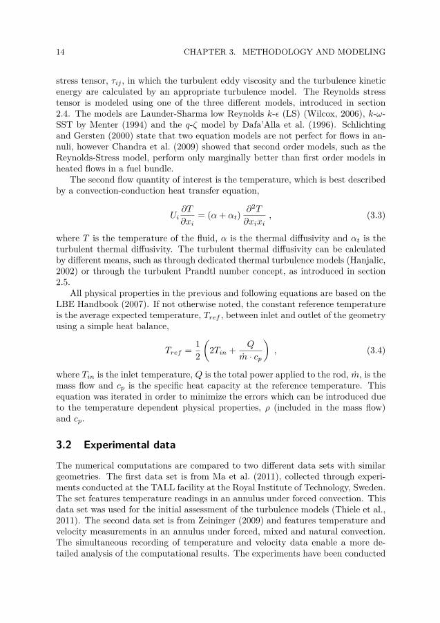
3.1 Schematic of the modeled part of the experimental test sections. Thedimensions are given in Table 3.1. The measurement levels indication ismeasured from the start of the heated section. . . . . . . . . . . . . . . 15
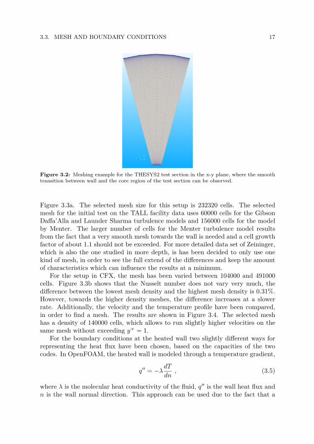
3.2 Meshing example for the THESYS2 test section in the x-y plane, wherethe smooth transition between wall and the core region of the test sectioncan be observed. . . . . . . . . . . . . . . . . . . . . . . . . . . . . . . . 17
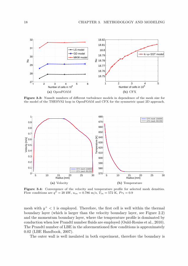
3.3 Nusselt numbers of different turbulence models in dependence of themesh size for the model of the THESYS2 loop in OpenFOAM and CFXfor the symmetric quasi 2D approach. . . . . . . . . . . . . . . . . . . . 18
3.4 Convergence of the velocity and temperature profile for selected meshdensities. Flow conditions are q′′ = 20 kW, uin = 0.786 m/s, Tin = 572K, Prt = 0.9 . . . . . . . . . . . . . . . . . . . . . . . . . . . . . . . . . 18
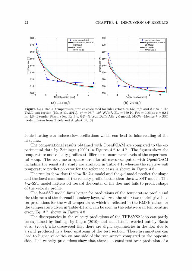
4.1 Radial temperature profiles calculated for inlet velocities 1.55 m/s and2 m/s in the TALL test section (Ma et al., 2011). q′′ = 93.7 ·104 W/m2,Tin = 579 K, Prt = 0.85 at z = 0.87 m. LS=Launder-Sharma low Rek-ε, GD=Gibson Daffa’Alla q-ζ model, MKW=Menter k-ω-SST model.Taken from Thiele and Anglart (2013). . . . . . . . . . . . . . . . . . . . 22
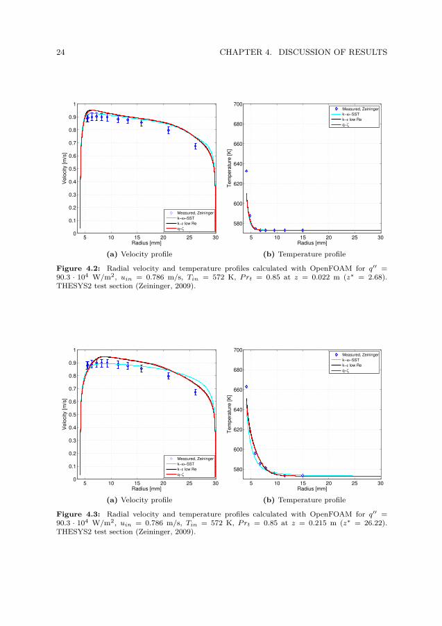
4.2 Radial velocity and temperature profiles calculated with OpenFOAMfor q′′ = 90.3 · 104 W/m2, uin = 0.786 m/s, Tin = 572 K, Prt = 0.85 atz = 0.022 m (z∗ = 2.68). THESYS2 test section (Zeininger, 2009). . . . 24
4.3 Radial velocity and temperature profiles calculated with OpenFOAMfor q′′ = 90.3 · 104 W/m2, uin = 0.786 m/s, Tin = 572 K, Prt = 0.85 atz = 0.215 m (z∗ = 26.22). THESYS2 test section (Zeininger, 2009). . . . 24
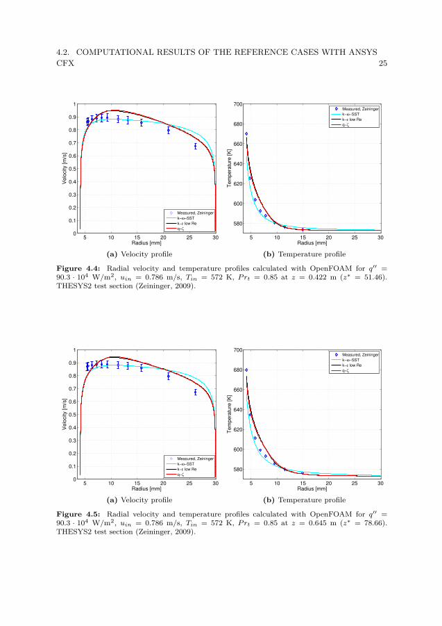
4.4 Radial velocity and temperature profiles calculated with OpenFOAMfor q′′ = 90.3 · 104 W/m2, uin = 0.786 m/s, Tin = 572 K, Prt = 0.85 atz = 0.422 m (z∗ = 51.46). THESYS2 test section (Zeininger, 2009). . . . 25
xi
xii List of Figures
4.5 Radial velocity and temperature profiles calculated with OpenFOAMfor q′′ = 90.3 · 104 W/m2, uin = 0.786 m/s, Tin = 572 K, Prt = 0.85 atz = 0.645 m (z∗ = 78.66). THESYS2 test section (Zeininger, 2009). . . . 25
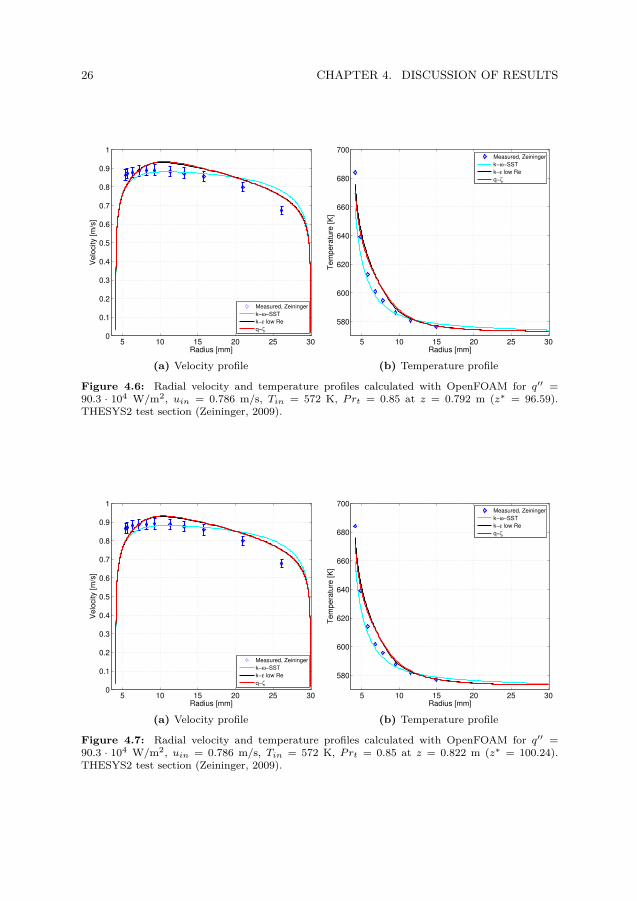
4.6 Radial velocity and temperature profiles calculated with OpenFOAMfor q′′ = 90.3 · 104 W/m2, uin = 0.786 m/s, Tin = 572 K, Prt = 0.85 atz = 0.792 m (z∗ = 96.59). THESYS2 test section (Zeininger, 2009). . . . 26
4.7 Radial velocity and temperature profiles calculated with OpenFOAMfor q′′ = 90.3 · 104 W/m2, uin = 0.786 m/s, Tin = 572 K, Prt = 0.85 atz = 0.822 m (z∗ = 100.24). THESYS2 test section (Zeininger, 2009). . . 26
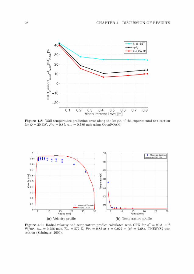
4.8 Wall temperature prediction error along the length of the experimen-tal test section for Q = 20 kW, Prt = 0.85, uin = 0.786 m/s usingOpenFOAM. . . . . . . . . . . . . . . . . . . . . . . . . . . . . . . . . . 28
4.9 Radial velocity and temperature profiles calculated with CFX for q′′ =90.3 ·104 W/m2, uin = 0.786 m/s, Tin = 572 K, Prt = 0.85 at z = 0.022m (z∗ = 2.68). THESYS2 test section (Zeininger, 2009). . . . . . . . . . 28
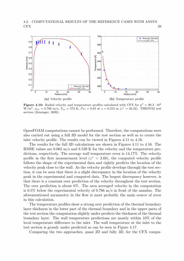
4.10 Radial velocity and temperature profiles calculated with CFX for q′′ =90.3 ·104 W/m2, uin = 0.786 m/s, Tin = 572 K, Prt = 0.85 at z = 0.215m (z∗ = 26.22). THESYS2 test section (Zeininger, 2009). . . . . . . . . 29
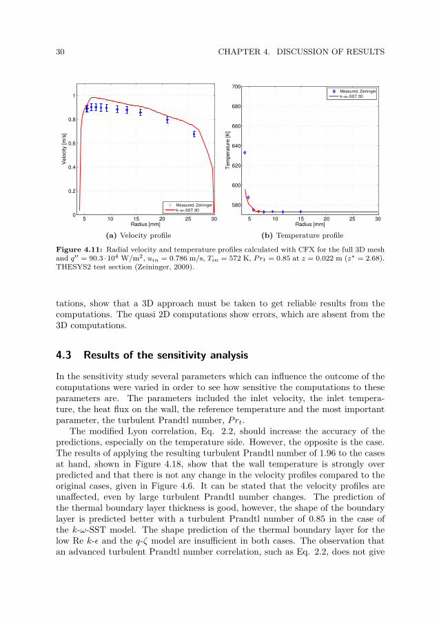
4.11 Radial velocity and temperature profiles calculated with CFX for thefull 3D mesh and q′′ = 90.3 · 104 W/m2, uin = 0.786 m/s, Tin = 572K, Prt = 0.85 at z = 0.022 m (z∗ = 2.68). THESYS2 test section(Zeininger, 2009). . . . . . . . . . . . . . . . . . . . . . . . . . . . . . . . 30
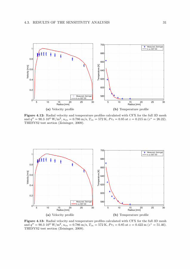
4.12 Radial velocity and temperature profiles calculated with CFX for thefull 3D mesh and q′′ = 90.3 · 104 W/m2, uin = 0.786 m/s, Tin = 572K, Prt = 0.85 at z = 0.215 m (z∗ = 26.22). THESYS2 test section(Zeininger, 2009). . . . . . . . . . . . . . . . . . . . . . . . . . . . . . . . 31
4.13 Radial velocity and temperature profiles calculated with CFX for thefull 3D mesh and q′′ = 90.3 · 104 W/m2, uin = 0.786 m/s, Tin = 572K, Prt = 0.85 at z = 0.422 m (z∗ = 51.46). THESYS2 test section(Zeininger, 2009). . . . . . . . . . . . . . . . . . . . . . . . . . . . . . . . 31
4.14 Radial velocity and temperature profiles calculated with CFX for thefull 3D mesh and q′′ = 90.3 · 104 W/m2, uin = 0.786 m/s, Tin = 572K, Prt = 0.85 at z = 0.645 m (z∗ = 78.66). THESYS2 test section(Zeininger, 2009). . . . . . . . . . . . . . . . . . . . . . . . . . . . . . . . 32
4.15 Radial velocity and temperature profiles calculated with CFX for thefull 3D mesh and q′′ = 90.3 · 104 W/m2, uin = 0.786 m/s, Tin = 572K, Prt = 0.85 at z = 0.792 m (z∗ = 96.59). THESYS2 test section(Zeininger, 2009). . . . . . . . . . . . . . . . . . . . . . . . . . . . . . . . 32
4.16 Radial velocity and temperature profiles calculated with CFX for thefull 3D mesh and q′′ = 90.3 · 104 W/m2, uin = 0.786 m/s, Tin = 572K, Prt = 0.85 at z = 0.822 m (z∗ = 100.24). THESYS2 test section(Zeininger, 2009). . . . . . . . . . . . . . . . . . . . . . . . . . . . . . . . 33
List of Figures xiii
4.17 Wall temperature prediction error along the length of the experimentaltest section for Q = 20 kW, Prt = 0.85, uin = 0.786 m/s using ANSYSCFX and a full 3D mesh. . . . . . . . . . . . . . . . . . . . . . . . . . . 33
4.18 Radial velocity and temperature profiles calculated with OpenFOAMq′′ = 90.3 · 104 W/m2, uin = 0.786 m/s, Tin = 572 K, Prt = 1.96(Lyon correlation) at z = 0.792 m (z∗ = 96.59). THESYS2 test section(Zeininger, 2009). . . . . . . . . . . . . . . . . . . . . . . . . . . . . . . . 34
4.19 Radial temperature profiles for different Prandtl numbers with Open-FOAM q′′ = 90.3·104 W/m2, uin = 0.786 m/s, Tin = 572 K at z = 0.792m (z∗ = 96.59). THESYS2 test section (Zeininger, 2009). . . . . . . . . 35
4.20 Radial velocity profiles with different inlet velocities calculated withOpenFOAMq′′ = 90.3 ·104 W/m2, Tin = 572 K, Prt = 0.85 at z = 0.792m (z∗ = 96.59). THESYS2 test section (Zeininger, 2009). . . . . . . . . 36
4.21 Radial temperature profiles with different inlet velocities calculated withOpenFOAM q′′ = 90.3·104 W/m2, Tin = 572 K, Prt = 0.85 at z = 0.792m (z∗ = 96.59). THESYS2 test section (Zeininger, 2009). . . . . . . . . 37
4.22 Radial temperature profiles with different heat fluxes applied to theinner cylinder calculated with OpenFOAM Tin = 572 K, uin = 0.786m/s, Prt = 0.85 at z = 0.792 m (z∗ = 96.59). THESYS2 test section(Zeininger, 2009). . . . . . . . . . . . . . . . . . . . . . . . . . . . . . . . 38
4.23 Radial velocity and temperature profiles for different reference temper-atures calculated with OpenFOAM q′′ = 90.3 · 104 W/m2, uin = 0.786m/s, Tin = 572 K, Prt = 0.85 at z = 0.792 m (z∗ = 96.59). THESYS2test section (Zeininger, 2009). . . . . . . . . . . . . . . . . . . . . . . . . 39


List of Tables
2.1 Coefficients, auxiliary functions and terms of the three turbulence mod-els (Thiele and Anglart, 2013). . . . . . . . . . . . . . . . . . . . . . . . 10
3.1 Comparison of geometrical and experimental conditions of the TALLand THESYS2 facilities. . . . . . . . . . . . . . . . . . . . . . . . . . . . 16
3.2 Summary of all boundary conditions and mesh configurations for thedifferent experimental setups and codes. . . . . . . . . . . . . . . . . . . 19
4.1 RMSE values for velocity and temperature of the THESYS2 calcula-tions for inlet velocity 0.786 m/s inlet calculated with OpenFOAM. Theresults of the sensitivity study use a power of 20 kW. . . . . . . . . . . . 27
4.2 Wall temperature errors in the predictions for the THESYS2 look com-putations with an increase of the turbulent Prandtl number by 10% . . 35
xv


List of Symbols
Symbol Dimensions DescriptionLatin Symbols
cp J/kg/K Specific heat capacitydrod m Rod diameterdpipe m Pipe diameterDΦ variable Destruction term for various propertiesgi m/s2 Gravitational acceleration vectorh W/m2/K Heat transfer coefficientk m2/s2 Turbulence kinetic energylheat m Heated lengthlinlet m Inlet lengthm kg/s Mass flow raten m Wall normal directionN Total number of cellsNu Nusselt numberRe Reynolds numberP Pa PressurePΦ variable Production term for various propertiesPe Peclet numberPr Prandtl numberQ W Heatq′′ W/m2 Heat fluxq m/s Square root of the turbulence kinetic energySij Mean strain rate tensorT K or ◦C TemperatureT ′ K or ◦C Temperature fluctuationTb K or ◦C Bulk temperatureTfilm K or ◦C Film temperatureTref K or ◦C Reference temperature
Continued on next page
xvii
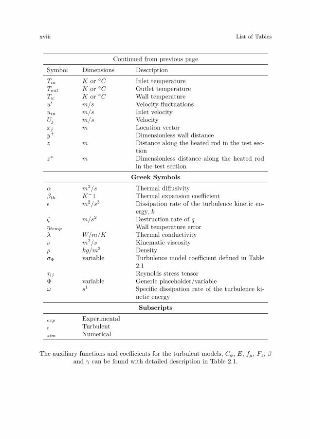
xviii List of Tables
Continued from previous pageSymbol Dimensions DescriptionTin K or ◦C Inlet temperatureTout K or ◦C Outlet temperatureTw K or ◦C Wall temperatureu′ m/s Velocity fluctuationsuin m/s Inlet velocityUj m/s Velocityxj m Location vectory+ Dimensionless wall distancez m Distance along the heated rod in the test sec-
tionz∗ m Dimensionless distance along the heated rod
in the test sectionGreek Symbols
α m2/s Thermal diffusivityβth K−1 Thermal expansion coefficientε m2/s3 Dissipation rate of the turbulence kinetic en-
ergy, kζ m/s2 Destruction rate of qηtemp Wall temperature errorλ W/m/K Thermal conductivityν m2/s Kinematic viscosityρ kg/m3 DensityσΦ variable Turbulence model coefficient defined in Table
2.1τij Reynolds stress tensorΦ variable Generic placeholder/variableω s1 Specific dissipation rate of the turbulence ki-
netic energySubscripts
exp Experimentalt Turbulentsim Numerical
The auxiliary functions and coefficients for the turbulent models, Cφ, E, fµ, F1, βand γ can be found with detailed description in Table 2.1.
Chapter 1
Introduction
Liquid metal cooled reactors have been proposed as one of several options for futureGeneration IV reactors. These kind of reactors will enable the sustainable and safeusage of nuclear energy (DOE, 2002). The goals for these next generation nuclearreactors are that they are sustainable in terms of responsible usage of resourcesas well as recycling of their own waste, economic in terms of being either cheaperor at least as economic as other sources of energy and safer, compared to today’sreactors, including proliferation safety, and accident safety. Liquid metal cooledreactors are seen as a safe and reliable option (Wallenius et al., 2012).
The goals for these reactors can only be achieved if the tools to design suchare available. Over the past years, the interest in these reactors and developmentof designs has picked up, as can be seen from different large projects investigatingdesigns and designing liquid metal cooled reactors, such as the THINS project(Roelofs et al., 2011), the MEGAPIE project (Fazio et al., 2008) or the ELECTRAproject (Wallenius et al., 2012).
This work focuses on the thermal hydraulics for liquid metal cooled reactor.Heat transfer in liquid metal cooled reactors is different from heat transfer in currentreactor designs, which employ mainly water as a coolant LBE Handbook (2007).This means that tools and models, which have been mainly developed for thermalhydraulics in water, must be validated and verified before they can be used in thedesign process of these next generation reactors.
This work aims at further the verification process for heat transfer in liquidmetal by using commercially available codes. These codes are tested against datawhich is available in the open literature, investigating how different turbulencemodels influence the prediction capabilities of these code.
The code that is mainly investigated in this work is OpenFOAM and three ofits available turbulence models. The second code studied is ANSYS CFX withone of its available turbulence models. The chapter on theoretical background willcover an introduction to liquid metal cooled reactors and properties of low Prandtlnumber fluids. It will explain the challenges which come with those fluids when
1
2 CHAPTER 1. INTRODUCTION
treating them numerically. The different turbulence models used in this work areintroduced, as well as how heat transfer is modeled in computational fluid dynamics(CFD).
The chapter on methodology and modeling will give an insight into the exper-imental data which has been used to compare the computations with. It will layout how the different turbulence models and the code are evaluated and analyzed.Following this, the results of the computations for the codes are presented andanalyzed based on the aforementioned methodology.
The conclusions close this work and will give ideas on future work and contin-uation of this work.
In order to understand subject at hand, the reader should have a basic un-derstanding of fluid dynamics and heat transfer, as well as a good knowledge ofmathematics.
1.1 Research objective
The main goal of this work is to investigate the predictive capabilities of turbulencemodels in a commercial code for forced convection flow of liquid lead-bismuth-eutectic (LBE) in annuli, investigate the influence each of these models has on thesepredictive capabilities and analyze the sensitivity to different input parameters.
Chapter 2
Theoretical Background
2.1 Liquid metal cooled reactors
In the road map for generation IV reactors published by the DOE (2002) liquidmetal cooled reactors are mentioned as one of the most versatile reactors as well asone of the options for actinide management, i.e. they are used to reduce nuclearwaste through fissioning it.
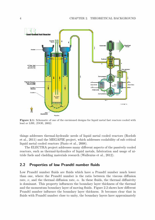
In Figure 2.1 a schematic of one of the proposed reactor designs with forcedconvection and in-vessel heat-exchangers/steam generators can be seen. This designis not the only one proposed. The options for liquid metal cooled reactors (lead andlead-bismuth-eutectic (LBE) cooled) range from 50 MWe and 150 MWe battery likereactors with very long refueling cycles to modular reactors, where each moduleproduces about 300 to 400 MWe. The largest designs envisioned produce 1200MWe and have the largest development potential, since they might also be usedfor hydrogen production when cladding material challenges have been overcome byR&D and high temperature materials for in-vessel use have been developed (DOE,2002).
Advantages of these reactors are the high sustainability rating through the closedfuel cycle for this kind of reactor (the conversion ratio is between 1 and 1.02).Additionally, this reactor class is proliferation resistant, because of its long fuel lifecycle, of up to 20 years. The good economy and safety rating is achieved throughthe ability to run these reactors on natural convection and the inert nature of thereactor coolant (DOE, 2002).
The disadvantages is that much research is needed on the material’s side in orderto manufacture materials for cladding and pumps, which sustain the prolongedexposure to radiation, high temperatures and LBE/lead flows.
For long term research goals, the production of hydrogen through process heatfrom the reactor is an option.
Liquid metal cooled reactor research needs are taken on by several different inter-national as well as national projects, such as the THINS project, which among other
3
4 CHAPTER 2. THEORETICAL BACKGROUND
Figure 2.1: Schematic of one of the envisioned designs for liquid metal fast reactors cooled withlead or LBE, (DOE, 2002)
things addresses thermal-hydraulic needs of liquid metal cooled reactors (Roelofset al., 2011) and the MEGAPIE project, which addresses coolability of sub criticalliquid metal cooled reactors (Fazio et al., 2008).
The ELECTRA project addresses many different aspects of the passively cooledreactors, such as thermal-hydraulics of liquid metals, fabrication and usage of ni-tride fuels and cladding materials research (Wallenius et al., 2012).
2.2 Properties of low Prandtl number fluids
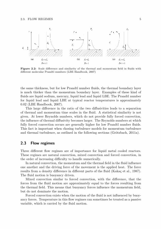
Low Prandtl number fluids are fluids which have a Prandtl number much lowerthan one, where the Prandtl number is the ratio between the viscous diffusionrate, ν, and the thermal diffusion rate, α. In these fluids, the thermal diffusivityis dominant. This property influences the boundary layer thickness of the thermaland the momentum boundary layer of moving fluids. Figure 2.2 shows how differentPrandtl number influence the boundary layer thickness. It becomes clear that influids with Prandtl number close to unity, the boundary layers have approximately
2.3. FLOW REGIMES 5
Figure 2.2: Scale difference and similarity of the thermal and momentum field in fluids withdifferent molecular Prandtl numbers (LBE Handbook, 2007)
.
the same thickness, but for low Prandtl number fluids, the thermal boundary layeris much thicker than the momentum boundary layer. Examples of these kind offluids are liquid sodium, mercury, liquid lead and liquid LBE. The Prandtl numberfor liquid lead and liquid LBE at typical reactor temperatures is approximately0.02 (LBE Handbook, 2007).
This large difference in the ratio of the two diffusivities leads to a separationof thermal and momentum time scales in the fluid. A statistical similarity is notgiven. At lower Reynolds numbers, which do not provide fully forced convection,the influence of thermal diffusivity becomes larger. The Reynolds numbers at whichfully forced convection occurs are generally higher for low Prandtl number fluids.This fact is important when chosing turbulence models for momentum turbulenceand thermal turbulence, as outlined in the following sections (Grötzbach, 2011a).
2.3 Flow regimes
Three different flow regimes are of importance for liquid metal cooled reactors.These regimes are natural convection, mixed convection and forced convection, inthe order of increasing difficulty to handle numerically.
In natural convection, the momentum and the thermal field in the fluid influenceone another and the driving force of the movement is the applied heat. The forceresults from a density difference in different parts of the fluid (Kakaç et al., 1987).The fluid motion is buoyancy driven.
Mixed convection similar to forced convection, with the difference, that theforces from the fluid motion are approximately equal to the forces resulting fromthe thermal field. This means that buoyancy forces influence the momentum field,but do not dominate the motion.
Forced convection exists when the motion of the fluid is not influenced by buoy-ancy forces. Temperature in this flow regimes can sometimes be treated as a passivevariable, which is carried by the fluid motion.
6 CHAPTER 2. THEORETICAL BACKGROUND
In order to predict which convection regime is present, different models can beapplied. These models were applied by the experimentalists to their data (Zeininger,2009). The author selected only experiments which were conducted in purely forcedconvective regime. This choice is motivated by the combination of RANS (Reynoldsaveraged Navier Stokes) turbulence models with a constant turbulent Prandtl num-ber (see section 2.4) and the knowledge that these kind of models are not able topredict mixed and/or natural convection without further modification.
2.3.1 Turbulent Prandtl number concept
The turbulent Prandtl number concept is also called Reynolds analogy and usesthe fact that for fluids such as water, the molecular Prandtl number is close tounity and the momentum and the thermal field are therefore similar, as shown inFigure 2.2. The Reynolds analogy makes use of this fact and relates the turbulencequantities, turbulent eddy viscosity and turbulent thermal diffusivity through asimple relation,
αt = νtPrt
, (2.1)
where Prt is the turbulent Prandtl number. In most cases this number is keptconstant throughout the computations.
For fluids whose molecular Prandtl number is close to unity, this holds very well,however, it has been shown that especially for strongly buoyant flows and mixedconvection flows (Grötzbach, 2011a), this relation produces erroneous temperaturefield predictions.
Several correlations for turbulent Prandtl number exist and have been tested inflows with low Prandtl number fluids (Baumann et al., 2011). The results of thesecalculations show that these correlations in their current form do not significantlyincrease the accuracy of thermal field predictions.
In the current investigation the feasibility of current commercial and open sourcecodes without modification are investigated and no varying turbulent Prandtl num-ber concepts are employed. However, one correlation by Lyon modified by Chengand Tak (2006) is used to set the fixed turbulent Prandtl number, Prt,
Prt = 0.01Pe[0.018Pe0.8 − (0.7−A)]1.25 , (2.2)
where Pe is the Peclet number, and A = 3.6 is a coefficient specified by the flowregime Peclet number, Pe ≥ 2000. The resulting turbulent Prandtl number is 1.96and is employed in the sensitivity analysis of the results, see section 3.4.
2.4. TURBULENCE MODELS 7
2.4 Turbulence models
Closure of the RANS equations is achieved through usage of turbulence models.The Reynolds stress tensor,
τij = 2νtSij + 23kδij , (2.3)
where νt is the kinematic turbulent eddy viscosity, Sij is the mean strain ratetensor and k the turbulence kinetic energy, needs to be modeled by some kind ofturbulence modeling. The chosen route in this study is the usage of first ordertwo-equation RANS turbulence models. Categorization of the models can be donetwo ways. One is categorizing them by high and low Reynolds number approaches,where high and low Reynolds number do not refer to the flow regime but to effectsclose to the wall. High Reynolds number models employ wall functions in order toset the velocity in the first wall adjacent cell (30 ≤ y+ ≤ 150) and avoid integratingthe momentum equation through the viscous sublayer. In contrast, low Reynoldsnumber models take the effects close to the wall into account and integrate thesolution through the viscous sublayer up to the wall (Schlichting and Gersten,2000). In this study only low Reynolds number approaches are used due to thenature of the flow as suggested by Ma et al. (2011). The second categorizationwhich can be made is the set of equations that the models use. On the one handthere are the k-ε class of equations, which also include the q-ζ model and on theother hand the k-ω models, including the original k-ω model by Wilcox (2006) andthe modified k-ω-SST model by Menter (1994). As can be seen from the names ofthe models, different approaches for the dissipation of the turbulent kinetic energy,k, are employed.
The two different codes have a slightly different set of turbulence models avail-able. OpenFOAM has the larger selection of k-ε type models and several k-ω typemodels are available, whereas CFX usage is restricted (for low Reynolds numberapproaches with first order two equation models) to k-ω type models. The modelsare explained in the following sub sections. Of these models all three are availablein OpenFOAM (OpenCFD Ltd (ESI Group), 2011), but only the k-ω-SST modelis available in CFX (ANSYS, 2012). The implementation of the models in Open-FOAM has been checked and verified using the source code guide to be consistentwith the models listed in the following sections (OpenFOAM, 2013).
2.4.1 Launder-Sharma low Reynolds k-ε model
In order to improve the behavior of the standard k-ε model for wall bounded flows,damping functions and a modification of the dissipation rate in the k-equationhave been performed by Launder and Sharma (Wilcox, 2006). The equation for theturbulence kinetic energy is very similar to the one used in the approach taken by
8 CHAPTER 2. THEORETICAL BACKGROUND
Menter (1994) for the k-ω-SST model,
Uj∂k
∂xj−(ν + νt
σk
)∂2k
∂xjxj= Pk −Dk , (2.4)
where ν is the kinematic molecular viscosity. The production of turbulence kineticenergy and the dissipation of turbulence kinetic energy, Pk and Dk, as well as themodeling coefficient σk are given in table 2.1.
The k-εmodeling approach is closed by the transport equation for the dissipationrate of the turbulence kinetic energy, ε,
Uj∂ε
∂xj= ∂
∂xj
[(νtσε
+ ν
)∂ε
∂xj
]+ Pε −Dε + E , (2.5)
where the Pε and Dε are the production and dissipation of ε, respectively. Thecoefficient σε, the production term, the dissipation term and the additional dampingfunction, E, are described in Table 2.1.
The turbulence eddy viscosity in the Launder-Sharma low Reynolds number k-εmodel is a for low Reynolds number effects modified version of νt,
νt = Cµfµk2
ε, (2.6)
where the coefficient Cµ and the damping function fµ are given in Table 2.1. Thismodel is only available in OpenFOAM and can therefore only be tested in this code.
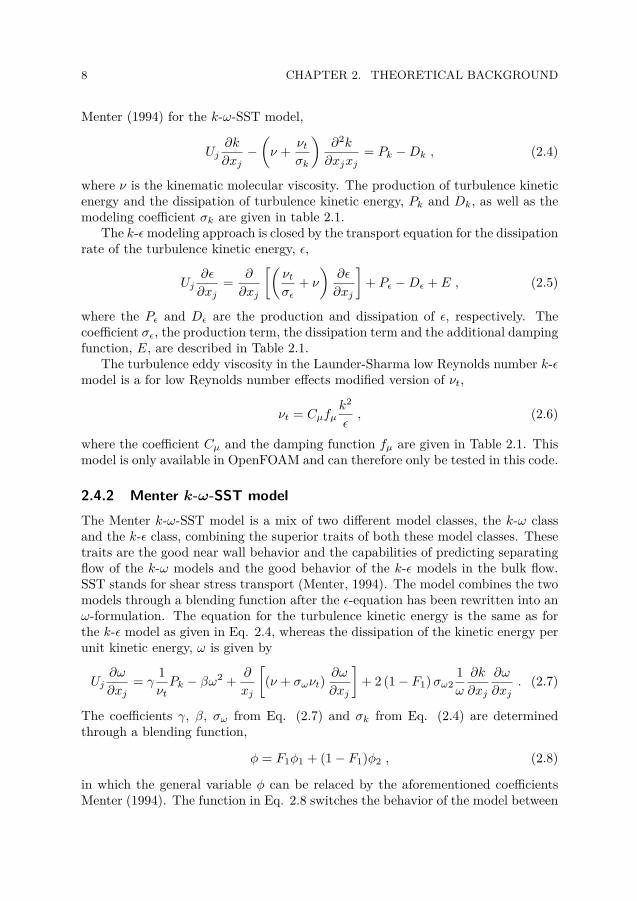
2.4.2 Menter k-ω-SST modelThe Menter k-ω-SST model is a mix of two different model classes, the k-ω classand the k-ε class, combining the superior traits of both these model classes. Thesetraits are the good near wall behavior and the capabilities of predicting separatingflow of the k-ω models and the good behavior of the k-ε models in the bulk flow.SST stands for shear stress transport (Menter, 1994). The model combines the twomodels through a blending function after the ε-equation has been rewritten into anω-formulation. The equation for the turbulence kinetic energy is the same as forthe k-ε model as given in Eq. 2.4, whereas the dissipation of the kinetic energy perunit kinetic energy, ω is given by
Uj∂ω
∂xj= γ
1νtPk − βω2 + ∂
xj
[(ν + σωνt)
∂ω
∂xj
]+ 2 (1− F1)σω2
1ω
∂k
∂xj
∂ω
∂xj. (2.7)
The coefficients γ, β, σω from Eq. (2.7) and σk from Eq. (2.4) are determinedthrough a blending function,
φ = F1φ1 + (1− F1)φ2 , (2.8)
in which the general variable φ can be relaced by the aforementioned coefficientsMenter (1994). The function in Eq. 2.8 switches the behavior of the model between

2.5. CFD MODELING OF HEAT TRANSFER 9
near wall k-ω modeling and bulk flow turbulence k-ε modeling. The coefficients, β,γ, σk and σε , for this model can be found in Table 2.1.
The turbulent kinetic eddy viscosity of this model is simply νt = kω, withoutany further damping functions and/or model coefficients.
The Menter k-ω-SST model is available in both codes, OpenFOAM and CFX.
2.4.3 Gibson Daffa’Alla q-ζ modelThe Gibson and Daffa’Alla q-ζ turbulence model is a low Reynolds number turbu-lence model and a reformulation of the classic low Reynolds number k-ε turbulencemodel, eliminating the dependence of k and ε on y2 close to the wall (Gibson andDafa’Alla, 1995). It uses the approaches by Jones and Launder and by Launderand Sharma (see section 2.4.1) for the damping functions and to determine the finalmodel coefficients. The model makes use of q =
√k and the rate of destruction of
q, ζ = ε/2q, which results in
Ui∂q
∂xi= ∂
∂xj
[(ν + νt
σq
)∂q
∂xj
]+ νt
2qSij∂Ui∂xj− ζ (2.9)
for q and in
Ui∂ζ
∂xi= ∂
∂xj
[(ν + νt
σζ
)∂ζ
∂xj
]+ ζ
q
(Cζ1fζ1
νt2qSij
∂Ui∂xj− Cζ2fζ2ζ
)+ ψ′ (2.10)
for ζ, respectively. The coefficients, σq and σζ and the damping functions Cζ1, Cζ2,fζ1, fζ2 and ψ′ can be found in Table 2.1.
The turbulent eddy viscosity for this model is given by
νt = Cµfµq3
2ζ , (2.11)
where the coefficient Cµ and the damping function fµ are given in Table 2.1.This model is only available in OpenFOAM.
2.5 CFD modeling of heat transfer
In most non-adiabatic CFD computations, two equation RANS models are used incombination with the turbulent Prandtl number concept, in which the turbulentthermal diffusivity is linked to the turbulent eddy diffusivity by a simple ratio,the turbulent Prandtl number (Grötzbach, 2011b). According to Schlichting andGersten (2000), the concept was developed for close to unity Prandtl number fluids,which possess similar scales for the thermal and momentum field. As mentionedearlier, in low Prandtl number fluids, this similarity does not exist and especiallyin mixed and natural convection, this fact will lead to problems using these kind ofmodels. Bricteux et al. (2012) mention, that even for forced convection, the usageof the turbulent Prandtl number concept needs to be applied with care.
10 CHAPTER 2. THEORETICAL BACKGROUND
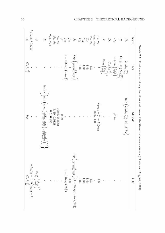
Table
2.1:Coeffi
cients,auxiliaryfunctions
andterm
softhe
threeturbulence
models
(Thiele
andAnglart,2013).
Term
LS
MK
WG
D
Pk
2νt Sij∂U
i∂x
jmin (2
νt Sij∂U
i∂x
j,10
·β∗kω )
-Pε
Cε1 f
ε1 νtεkSij∂U
i∂x
j-
-
Dk
ε+2ν (
∂√k
∂y )
2β∗kω
-
Dε
Cε2 f
ε2ε 2k
--
E2ννt (
∂U
i
∂x
2j )2
--
σk ,σq
1F
1 σk1
+(1
−F
1 )σk2
1.0σk1 ,
σk2
-0.85,1.0
-σe ,σθ
1.3-
1.3Cε1
1.44-
1.44Cε2
1.92-
1.92Cµ
0.09-
0.09fµ
exp (−
3.4
(1+Re
t/50) 2 )
-exp (
−6
(1+Re
t/50) 2 )
(1+
3exp[−Reτ/10])
fε1
1-
1.0fε2
1−
0.3exp (−
Re
2t )-
1−
0.3exp(R
e2t )
β∗
-0.09
-γ
1 ,γ
2-
0.856,0.5532-
β1 ,β
2-
3/40,0.0828-
σω
1 ,σω
2-
0.5,0.856-
F1
-tanh {[m
in (max (
√k
β∗ωy,
500ν
y2ω )
,4σ
ω2k
CD
kωy
2 )]4 }
-
ψ′
--
2νν
t2q (
∂2U
i
∂x
2j )2
Cζ1 f
ζ1 ,Cζ2 f
ζ2-
-2Cε1 f
ε1−
1,2Cε2 f
ε2−
1νt
Cµfµk
2εkω
Cµfµq
3
2ζ
2.5. CFD MODELING OF HEAT TRANSFER 11
Kakaç et al. (1987) give the turbulent Prandtl number as
Prt = νt
u′T ′∂T
∂x= νtαt
, (2.12)
where 1/u′T ′∂T/∂x is replaced with the turbulent thermal diffusivity αt. u′T ′
are the turbulent heat fluxes, resulting from Reynolds averaging the temperatureequation.
Several attempts have been made to overcome the problems related to the tur-bulent Prandtl number concept. The solutions range from modifying the turbulentPrandtl number through empirical or semi-empirical correlations dependent on flowparameters (Baumann et al., 2011) to full thermal turbulence models, such as the al-gebraic heat flux model (AHFM) (Pellegrini et al., 2011) or two and multi-equationmodels to describe the thermal and momentum turbulence in these flows (Carte-ciano and Grötzbach, 2003; Baumann et al., 2012). However, these models are notyet available in commercial codes and they have to be verified against experimentaland/or DNS data for most flow regimes.

Chapter 3
Methodology and Modeling
This chapter will introduce the methodology applied to this study. It begins with anintroduction of the governing equations that are solved using the two computationalfluid dynamics codes, OpenFOAM (vers. 2.1.1) (OpenCFD Ltd (ESI Group), 2011)and ANSYS CFX 14.5 (ANSYS, 2012). Furthermore, the experimental data ispresented before the modeling process of the two experimental setups is explained.The chapter ends with a short overview about the sensitivity analysis and how thenumerical data was evaluated.
3.1 Governing equations
The governing equations for the study is composed of two parts for the two differentfields that are evaluated, momentum and temperature field. The first part consistsof the RANS equation and the mass conservation equation for incompressible flowand constant transport properties,
Uj∂Ui∂xj
= −1ρ
∂P
∂xi+ ∂
∂xj[2νSij + τij ] + βthgi (T − Tref ) (3.1)
and∂Ui∂xi
= 0 , (3.2)
where Ui is the velocity, P is the pressure, ρ is density and τij is the Reynoldsstress tensor. The last term of equation (3.1) is the Boussinesq approximation forbuoyancy (Schlichting and Gersten, 2000), in which βth is the thermal expansioncoefficient, gi is the gravitational acceleration vector and (T − Tref ) is the tem-perature difference between the reference temperature and the local temperature.This last term predicts the local buoyancy forces based on the temperature differ-ence. The quantities Ui and T are Reynolds averaged quantities and represent timeaveraged quantities. The turbulent fluctuations which influence the flow throughadditional stress enter the momentum equation (Eq. (3.1)) through the Reynolds
13
14 CHAPTER 3. METHODOLOGY AND MODELING
stress tensor, τij , in which the turbulent eddy viscosity and the turbulence kineticenergy are calculated by an appropriate turbulence model. The Reynolds stresstensor is modeled using one of the three different models, introduced in section2.4. The models are Launder-Sharma low Reynolds k-ε (LS) (Wilcox, 2006), k-ω-SST by Menter (1994) and the q-ζ model by Dafa’Alla et al. (1996). Schlichtingand Gersten (2000) state that two equation models are not perfect for flows in an-nuli, however Chandra et al. (2009) showed that second order models, such as theReynolds-Stress model, perform only marginally better than first order models inheated flows in a fuel bundle.
The second flow quantity of interest is the temperature, which is best describedby a convection-conduction heat transfer equation,
Ui∂T
∂xi= (α+ αt)
∂2T
∂xixi, (3.3)
where T is the temperature of the fluid, α is the thermal diffusivity and αt is theturbulent thermal diffusivity. The turbulent thermal diffusivity can be calculatedby different means, such as through dedicated thermal turbulence models (Hanjalic,2002) or through the turbulent Prandtl number concept, as introduced in section2.5.
All physical properties in the previous and following equations are based on theLBE Handbook (2007). If not otherwise noted, the constant reference temperatureis the average expected temperature, Tref , between inlet and outlet of the geometryusing a simple heat balance,
Tref = 12
(2Tin + Q
m · cp
), (3.4)
where Tin is the inlet temperature, Q is the total power applied to the rod, m, is themass flow and cp is the specific heat capacity at the reference temperature. Thisequation was iterated in order to minimize the errors which can be introduced dueto the temperature dependent physical properties, ρ (included in the mass flow)and cp.
3.2 Experimental data
The numerical computations are compared to two different data sets with similargeometries. The first data set is from Ma et al. (2011), collected through experi-ments conducted at the TALL facility at the Royal Institute of Technology, Sweden.The set features temperature readings in an annulus under forced convection. Thisdata set was used for the initial assessment of the turbulence models (Thiele et al.,2011). The second data set is from Zeininger (2009) and features temperature andvelocity measurements in an annulus under forced, mixed and natural convection.The simultaneous recording of temperature and velocity data enable a more de-tailed analysis of the computational results. The experiments have been conducted
3.2. EXPERIMENTAL DATA 15
at the THESYS2 facility at KIT in Germany. Only forced convection is considereddue to the already known problems using a constant turbulent Prandtl number ap-proach for mixed and natural convection (Grötzbach, 2011a). For both setups, onlythe test section as shown in Figure 3.1 has been used in the modeling setup. Theexperimental data range is given in Table 3.1. Both experimental setups apply theheat flux at the inner cylinder and have adiabatic conditions at the outer cylinder.The outer cylinders are well insulated according to Zeininger (2009) and Ma et al.(2011), respectively. The flow is fully turbulent at the entry to the test section andstays turbulent throughout the test section.
(a) TALL (b) THESYS2
Figure 3.1: Schematic of the modeled part of the experimental test sections. The dimensions aregiven in Table 3.1. The measurement levels indication is measured from the start of the heatedsection.
In both cases the flow is vertically upwards under forced convection. Therefore,symmetry can be assumed. This leads to a simpler mesh and overall to a smallermesh, decreasing the required computational time.
The data set by Zeininger (2009) has been used for computations by Battaet al. (2009) and one source of error has been identified. The fluid passes througha bend before it enters the flow development pipe, which ensures fully developedflow in the test section. Vortices are introduced at the bend, which do not fullydissipate before reaching the test section, which leads to slightly asymmetric flow.The experiments have been repeated by Marocco et al. (2012) and the results arethe same.
16 CHAPTER 3. METHODOLOGY AND MODELING
Table 3.1: Comparison of geometrical and experimental conditions of the TALL and THESYS2facilities.
Property TALL (Ma et al., 2011) THESYS2 (Zeininger, 2009)
Inlet velocity, Uin [m/s] 0.65 .. 2.00 0.786Re 99100 .. 127000 310000Heat flux, q′′ [W/m2] 93.7·104 13.5·104 .. 90.3·104
Inlet temp., Tin [K] ∼579 572Outlet temp., Tout [K] 609 .. 672 574 .. 579Rod diameter, drod [mm] 8.2 8.2Pipe diameter, dpipe [mm] 19.0 60.0Heated length, lheat [mm] 870 860Inlet length, linlet [mm] 1000 59
The measurements in both cases have been taken in radial direction at differentlevels along the flow path. In the THESYS2 measurements, additionally to thetemperature measurements, the flow velocity has been recorded. The measurementsin the TALL facility were taken in 4 different levels between the start of the heatedrod section and the outlet through fixed rakes which recorded the temperature in4 points in the radial direction (Ma et al., 2011) as indicated in Figure 3.1a. Inthe THESYS2 experimental setup measurements were taken on 6 different levelsbetween inlet and outlet. The measurements were taken on fixed rakes and amoveable sled, which also held a pitot tube. The schematic in Figure 3.1b showsthe different measurement levels and the experimental test section dimensions.
3.3 Mesh and boundary conditions
The nature of the flow, vertically upwards and forced convection, leads to theassumption that 3D effects can be neglected and that the flow can be modeledusing symmetry in a quasi 2D approach. This leads to the the modeling of onlya small slice of the geometry, reducing mesh size and computational time. Allmeshes employed are purely hexagonal structured meshes, which have a smoothtransition from the walls to the center of the flow domain. An example of themeshing structure in the x-y plane is given in Figure 3.2. All meshes are limited toy+ < 1 for the first grid point.
Before any meaningful computations can be carried out, a mesh independencestudy needs to be carried out to find the mesh on which the computations arerun. The approach taken here is similar to the one taken by Natesan et al. (2010).It cannot be assured that the implementation of the numerical schemes and theimplementation of the turbulence models are the same for both codes. Therefore,different meshes are employed, according to the mesh independence study. ForOpenFOAM a mesh independence study was carried out by varying the amountof cells between 158400 and 576000 for the THESYS2 setup, which can be seen in
3.3. MESH AND BOUNDARY CONDITIONS 17
Figure 3.2: Meshing example for the THESYS2 test section in the x-y plane, where the smoothtransition between wall and the core region of the test section can be observed.
Figure 3.3a. The selected mesh size for this setup is 232320 cells. The selectedmesh for the initial test on the TALL facility data uses 60000 cells for the GibsonDaffa’Alla and Launder Sharma turbulence models and 156000 cells for the modelby Menter. The larger number of cells for the Menter turbulence model resultsfrom the fact that a very smooth mesh towards the wall is needed and a cell growthfactor of about 1.1 should not be exceeded. For more detailed data set of Zeininger,which is also the one studied in more depth, is has been decided to only use onekind of mesh, in order to see the full extend of the differences and keep the amountof characteristics which can influence the results at a minimum.
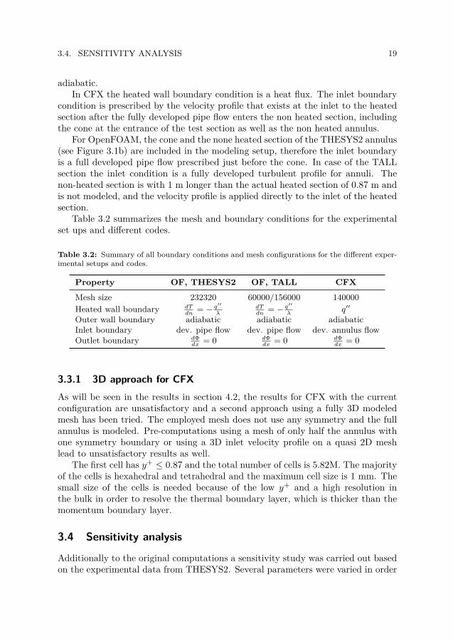
For the setup in CFX, the mesh has been varied between 104000 and 491000cells. Figure 3.3b shows that the Nusselt number does not vary very much, thedifference between the lowest mesh density and the highest mesh density is 0.31%.However, towards the higher density meshes, the difference increases at a slowerrate. Additionally, the velocity and the temperature profile have been compared,in order to find a mesh. The results are shown in Figure 3.4. The selected meshhas a density of 140000 cells, which allows to run slightly higher velocities on thesame mesh without exceeding y+ = 1.
For the boundary conditions at the heated wall two slightly different ways forrepresenting the heat flux have been chosen, based on the capacities of the twocodes. In OpenFOAM, the heated wall is modeled through a temperature gradient,
q′′ = −λdTdn
, (3.5)
where λ is the molecular heat conductivity of the fluid, q′′ is the wall heat flux andn is the wall normal direction. This approach can be used due to the fact that a
18 CHAPTER 3. METHODOLOGY AND MODELING
1 2 3 4 5 627
28
29
30
31
32
Number of cells in 105
Nu
LS model
GD model
MKW model
(a) OpenFOAM
1 2 3 4 5
18.75
18.76
18.77
18.78
18.79
18.8
18.81
18.82
Number of cells in 105
Nu
k−ω−SST model
(b) CFX
Figure 3.3: Nusselt numbers of different turbulence models in dependence of the mesh size forthe model of the THESYS2 loop in OpenFOAM and CFX for the symmetric quasi 2D approach.
5 10 15 20 25 300
0.1
0.2
0.3
0.4
0.5
0.6
0.7
0.8
0.9
1
Radius [mm]
Vel
ocity
[m/s
]
CFX mesh 104000CFX mesh 491200
(a) Velocity
5 10 15 20 25 30570
580
590
600
610
620
630
640
650
660
670
680
Radius [mm]
Tem
pera
ture
[K]
CFX mesh 104000CFX mesh 491200
(b) Temperature
Figure 3.4: Convergence of the velocity and temperature profile for selected mesh densities.Flow conditions are q′′ = 20 kW, uin = 0.786 m/s, Tin = 572 K, Prt = 0.9
mesh with y+ < 1 is employed. Therefore, the first cell is well within the thermalboundary layer (which is larger than the velocity boundary layer, see Figure 2.2)and the momentum boundary layer, where the temperature profile is dominated byconduction when low Prandtl number fluids are employed (Ould-Rouiss et al., 2010).The Prandtl number of LBE in the aforementioned flow conditions is approximately0.02 (LBE Handbook, 2007).
The outer wall is well insulated in both experiment, therefore the boundary is
3.4. SENSITIVITY ANALYSIS 19
adiabatic.In CFX the heated wall boundary condition is a heat flux. The inlet boundary
condition is prescribed by the velocity profile that exists at the inlet to the heatedsection after the fully developed pipe flow enters the non heated section, includingthe cone at the entrance of the test section as well as the non heated annulus.
For OpenFOAM, the cone and the none heated section of the THESYS2 annulus(see Figure 3.1b) are included in the modeling setup, therefore the inlet boundaryis a full developed pipe flow prescribed just before the cone. In case of the TALLsection the inlet condition is a fully developed turbulent profile for annuli. Thenon-heated section is with 1 m longer than the actual heated section of 0.87 m andis not modeled, and the velocity profile is applied directly to the inlet of the heatedsection.
Table 3.2 summarizes the mesh and boundary conditions for the experimentalset ups and different codes.
Table 3.2: Summary of all boundary conditions and mesh configurations for the different exper-imental setups and codes.
Property OF, THESYS2 OF, TALL CFX
Mesh size 232320 60000/156000 140000Heated wall boundary dT
dn= − q′′
λdTdn
= − q′′
λq′′
Outer wall boundary adiabatic adiabatic adiabaticInlet boundary dev. pipe flow dev. pipe flow dev. annulus flowOutlet boundary dΦ
dx= 0 dΦ
dx= 0 dΦ
dx= 0
3.3.1 3D approach for CFXAs will be seen in the results in section 4.2, the results for CFX with the currentconfiguration are unsatisfactory and a second approach using a fully 3D modeledmesh has been tried. The employed mesh does not use any symmetry and the fullannulus is modeled. Pre-computations using a mesh of only half the annulus withone symmetry boundary or using a 3D inlet velocity profile on a quasi 2D meshlead to unsatisfactory results as well.
The first cell has y+ ≤ 0.87 and the total number of cells is 5.82M. The majorityof the cells is hexahedral and tetrahedral and the maximum cell size is 1 mm. Thesmall size of the cells is needed because of the low y+ and a high resolution inthe bulk in order to resolve the thermal boundary layer, which is thicker than themomentum boundary layer.
3.4 Sensitivity analysis
Additionally to the original computations a sensitivity study was carried out basedon the experimental data from THESYS2. Several parameters were varied in order
20 CHAPTER 3. METHODOLOGY AND MODELING
to see how large the influence of these parameters is. The inlet temperature (±1%),the inlet velocity (±5%), the heat flux (±5%) and the turbulent Prandtl numberwere varied (±10%). Additionally to the increase and decrease of the turbulentPrandtl number, a Prandtl number correlation for a fixed Prandtl number basedon the Lyon Prandtl number correlation, but modified by Cheng and Tak (2006)was used, as introduced in Eq. 2.2.
As mentioned before, the computations are carried out using a constant refer-ence temperature, which is the average bulk temperature between inlet and outlet.The effect of the reference temperature is studied by using a different referencetemperature, the average film temperature, Tfilm,
Tfilm = Tw + Tb2 , (3.6)
where Tw and Tb are the wall and bulk temperature, respectively. However, it isclear that this method is difficult to implement without prior knowledge of the walltemperatures and and is impractical in flows where wall temperatures are not asimportant, such as temperature mixing problems.
3.5 Evaluation of the predictions
The results of the predictions and the sensitivity analysis need to be comparableto one another. Different ways of evaluation can be adopted. The first step is tovisually compare the obtained computational results with the experimental results.
One of the most important values that needs to be assessed is the wall temper-ature, because it determines one of the safety margins for reactors. The error inthe wall temperature is given by
ηtemp = Tw,exp − Tw,sim∆Tin,exp
, (3.7)
where Tw,exp and Tw,sim are the real wall temperature and the computed walltemperature, respectively. ∆Tin,exp is the temperature between the inlet and thetemperature at the experimental point in question. This way the relative temper-ature increase is taken into account in the error measurement.
The third and last step in the evaluation is to collapse the predictions intoone value, which makes ranking the results much easier. The chosen value is theroot mean square error (RMSE). The RMSE is taken for the velocity and thetemperature results respectively and covers all measurement points.
Chapter 4
Discussion of Results
The following sections describe the results found during the computations and com-pare these results to the experimental data found in Ma et al. (2011) and Zeininger(2009). Velocity and temperature profiles are compared and RMSE values and walltemperature prediction errors are shown for both codes.
4.1 Computational results of the reference cases withOpenFOAM
The first results presented here are the computations for the TALL test sectionwith OpenFOAM. The computations in the TALL section were used to initiallyseparate the different turbulence models from one another and determine for whichmodels more detailed computations should be carried out (Thiele et al., 2011). Thepresented temperature profiles are taken from Thiele and Anglart (2013) and showthe three different turbulence models, which gave the best predictions in the pre-investigation. The wall temperature is not part of the data set and it was thereforeapproximated through a simple heat transfer approach,
Tw = q′′/h+ Tb , (4.1)
using a heat transfer correlation by Dwyer (LBE Handbook, 2007, pp. 456, 457) forthe heat transfer coefficient h, which is applicable to fully developed liquid metalflow in an annulus. Tw and Tb are the wall and bulk temperature, respectively. Theheat flux is given by q′′. The three models give similar results, where the k-ω-SSTmodel gives a slightly better prediction of the bulk temperature.
Ma et al. (2011) give several sources, which can be attributed to the predictionerror in Figures 4.1a and 4.1b. One of the sources of error can be disturbances inthe flow due to the combination of the small annulus size of 5.4 mm across and thesize of the thermo-couple probe of 3 mm. The large thermo-couple probe can partlylead to the underprediction of the thermal boundary layer thickness. The methodto heat the rod, joule heating, can be another source of error in the measurements.
21
22 CHAPTER 4. DISCUSSION OF RESULTS
4 5 6 7 8 9600
610
620
630
640
650
660
670
680
Radial position [mm]
Te
mp
era
ture
[K
]
exp. extrapolated
Experimental, Ma et al.
LS Model
GD Model
MKW Model
(a) 1.55 m/s
4 5 6 7 8 9600
610
620
630
640
650
660
670
680
Radial position [mm]T
em
pe
ratu
re [
K]
exp. extrapolated
Experimental, Ma et al.
LS Model
GD Model
MKW Model
(b) 2.0 m/s
Figure 4.1: Radial temperature profiles calculated for inlet velocities 1.55 m/s and 2 m/s in theTALL test section (Ma et al., 2011). q′′ = 93.7 · 104 W/m2, Tin = 579 K, Prt = 0.85 at z = 0.87m. LS=Launder-Sharma low Re k-ε, GD=Gibson Daffa’Alla q-ζ model, MKW=Menter k-ω-SSTmodel. Taken from Thiele and Anglart (2013).
Joule heating can induce slow oscillations which can lead to false reading of theheat flux.
The computational results obtained with OpenFOAM are compared to the ex-perimental data by Zeininger (2009) in Figures 4.2 to 4.7. The figures show thetemperature and velocity profiles at different measurement levels of the experimen-tal setup. The root mean square error for all cases computed with OpenFOAMincluding the sensitivity study are available in Table 4.1, whereas the relative walltemperature prediction error for the reference cases is shown in Figure 4.8.
The results show that the low Re k-ε model and the q-ζ model predict the shapeand the local maximum of the velocity profile better than the k-ω-SST model. Thek-ω-SST model flattens off toward the center of the flow and fails to predict shapeof the velocity profile.
The k-ω-SST model fares better for predictions of the temperature profile andthe thickness of the thermal boundary layer, whereas the other two models give bet-ter predictions for the wall temperature, which is reflected in the RMSE values forthe temperature given in Table 4.1 and can be seen in the relative wall temperatureerror, Eq. 3.7, shown in Figure 4.8.
The discrepancies in the velocity predictions of the THESYS2 loop can partlybe explained by findings by Loges (2010) and calculations carried out by Battaet al. (2009), who discovered that there are slight asymmetries in the flow due toa swirl produced in a bend upstream of the test section. These asymmetries canlead to higher velocities on one side of the test section compared to the oppositeside. The velocity predictions show that there is a consistent over prediction of a
4.2. COMPUTATIONAL RESULTS OF THE REFERENCE CASES WITH ANSYSCFX 23
few percent points by all three models. However, it must be noted that the velocityprofile from the experimental data does not cover the near wall regions, whichdenies the possibility to calculate the average velocity in this part of test sectionfor comparison with the predicted data. However, in all computations, the averagevelocity at the outlet is within 0.5% of the in Zeininger (2009) reported velocities.
The asymmetry in the velocity profile can also be one of the error sourcesfor the temperature predictions, due to the fact that a lower flow velocity on themeasurement side, would also increase the wall temperature, which in return is thenunder predicted by the computations.
Other sources of error are the model assumptions applied to the calculations.One of the most common assumption for forced convection flow with small changesin density is the Boussinesq assumption for buoyant flow. The density differencebetween the highest and the reference temperature within the domain is 1.56%,which should not introduce any errors. Such a small difference shows that thisassumption is valid. Zeininger (2009) indicates that the flow regimes which werecomputed and compared in the current study are all forced convection. It is alsoclearly visible from the experimental and numerical results that the velocity profilesalong the experimental test section are not skewed or distorted, as it would beexpected with mixed or natural convection.
Choosing a fixed turbulent Prandtl number can be problematic, since the mo-mentum and thermal spectrum are not similar in the case of low Prandtl numberfluids, such as LBE (Grötzbach, 2011a). Kawamura et al. (1999) show that the Prtchanges throughout the flow field, with the largest changes occurring close to thewall. The assumption of a fixed turbulent Prandtl number can lead to errors in thewall temperature and thermal boundary layer thickness predictions. The relativewall temperature prediction error is shown in Figure 4.8, and the boundary layerthickness can be estimated from Figures 4.2 to 4.7. The thickness of the thermalboundary layer is slightly over predicted by the k-ω-SST model, but well predictedby the low Re k-ε model and the q-ζ model. The wall temperature show large errorsfor all three models, with the k-ω-SST model experiencing the largest errors.
The numerical schemes can lead to erroneous computations, as only first orderturbulence models are applied to the flow. Baumann (2012) notes that these kindof models are not capable of predicting the shift of the location of zero shear stresswith respect to the location of the maximum velocity, which are different from oneanother in annuli flow. However, the applied models are well tested and validatedthrough years of industrial and academic usage for a large range of flows and areknown to give sufficient results for even more complex flows.
4.2 Computational results of the reference cases with ANSYSCFX
The velocity and temperature profiles for the first two measurement levels computedwith ANSYS CFX in quasi 2D for the case of the THESYS2 test section with the
24 CHAPTER 4. DISCUSSION OF RESULTS
5 10 15 20 25 300
0.1
0.2
0.3
0.4
0.5
0.6
0.7
0.8
0.9
1
Radius [mm]
Ve
locity [
m/s
]
Measured, Zeininger
k−ω−SST
k−ε low Re
q−ζ
(a) Velocity profile
5 10 15 20 25 30
580
600
620
640
660
680
700
Radius [mm]
Te
mp
era
ture
[K
]
Measured, Zeininger
k−ω−SST
k−ε low Re
q−ζ
(b) Temperature profile
Figure 4.2: Radial velocity and temperature profiles calculated with OpenFOAM for q′′ =90.3 · 104 W/m2, uin = 0.786 m/s, Tin = 572 K, Prt = 0.85 at z = 0.022 m (z∗ = 2.68).THESYS2 test section (Zeininger, 2009).
5 10 15 20 25 300
0.1
0.2
0.3
0.4
0.5
0.6
0.7
0.8
0.9
1
Radius [mm]
Ve
locity [
m/s
]
Measured, Zeininger
k−ω−SST
k−ε low Re
q−ζ
(a) Velocity profile
5 10 15 20 25 30
580
600
620
640
660
680
700
Radius [mm]
Te
mp
era
ture
[K
]
Measured, Zeininger
k−ω−SST
k−ε low Re
q−ζ
(b) Temperature profile
Figure 4.3: Radial velocity and temperature profiles calculated with OpenFOAM for q′′ =90.3 · 104 W/m2, uin = 0.786 m/s, Tin = 572 K, Prt = 0.85 at z = 0.215 m (z∗ = 26.22).THESYS2 test section (Zeininger, 2009).
4.2. COMPUTATIONAL RESULTS OF THE REFERENCE CASES WITH ANSYSCFX 25
5 10 15 20 25 300
0.1
0.2
0.3
0.4
0.5
0.6
0.7
0.8
0.9
1
Radius [mm]
Ve
locity [
m/s
]
Measured, Zeininger
k−ω−SST
k−ε low Re
q−ζ
(a) Velocity profile
5 10 15 20 25 30
580
600
620
640
660
680
700
Radius [mm]
Te
mp
era
ture
[K
]
Measured, Zeininger
k−ω−SST
k−ε low Re
q−ζ
(b) Temperature profile
Figure 4.4: Radial velocity and temperature profiles calculated with OpenFOAM for q′′ =90.3 · 104 W/m2, uin = 0.786 m/s, Tin = 572 K, Prt = 0.85 at z = 0.422 m (z∗ = 51.46).THESYS2 test section (Zeininger, 2009).
5 10 15 20 25 300
0.1
0.2
0.3
0.4
0.5
0.6
0.7
0.8
0.9
1
Radius [mm]
Ve
locity [
m/s
]
Measured, Zeininger
k−ω−SST
k−ε low Re
q−ζ
(a) Velocity profile
5 10 15 20 25 30
580
600
620
640
660
680
700
Radius [mm]
Te
mp
era
ture
[K
]
Measured, Zeininger
k−ω−SST
k−ε low Re
q−ζ
(b) Temperature profile
Figure 4.5: Radial velocity and temperature profiles calculated with OpenFOAM for q′′ =90.3 · 104 W/m2, uin = 0.786 m/s, Tin = 572 K, Prt = 0.85 at z = 0.645 m (z∗ = 78.66).THESYS2 test section (Zeininger, 2009).
26 CHAPTER 4. DISCUSSION OF RESULTS
5 10 15 20 25 300
0.1
0.2
0.3
0.4
0.5
0.6
0.7
0.8
0.9
1
Radius [mm]
Ve
locity [
m/s
]
Measured, Zeininger
k−ω−SST
k−ε low Re
q−ζ
(a) Velocity profile
5 10 15 20 25 30
580
600
620
640
660
680
700
Radius [mm]
Te
mp
era
ture
[K
]
Measured, Zeininger
k−ω−SST
k−ε low Re
q−ζ
(b) Temperature profile
Figure 4.6: Radial velocity and temperature profiles calculated with OpenFOAM for q′′ =90.3 · 104 W/m2, uin = 0.786 m/s, Tin = 572 K, Prt = 0.85 at z = 0.792 m (z∗ = 96.59).THESYS2 test section (Zeininger, 2009).
5 10 15 20 25 300
0.1
0.2
0.3
0.4
0.5
0.6
0.7
0.8
0.9
1
Radius [mm]
Ve
locity [
m/s
]
Measured, Zeininger
k−ω−SST
k−ε low Re
q−ζ
(a) Velocity profile
5 10 15 20 25 30
580
600
620
640
660
680
700
Radius [mm]
Te
mp
era
ture
[K
]
Measured, Zeininger
k−ω−SST
k−ε low Re
q−ζ
(b) Temperature profile
Figure 4.7: Radial velocity and temperature profiles calculated with OpenFOAM for q′′ =90.3 · 104 W/m2, uin = 0.786 m/s, Tin = 572 K, Prt = 0.85 at z = 0.822 m (z∗ = 100.24).THESYS2 test section (Zeininger, 2009).
4.2. COMPUTATIONAL RESULTS OF THE REFERENCE CASES WITH ANSYSCFX 27
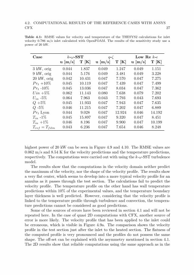
Table 4.1: RMSE values for velocity and temperature of the THESYS2 calculations for inletvelocity 0.786 m/s inlet calculated with OpenFOAM. The results of the sensitivity study use apower of 20 kW.
Case k-ω-SST q-ζ Low Re k-εu [m/s] T [K] u [m/s] T [K] u [m/s] T [K]
3 kW, orig 0.044 1.837 0.049 1.247 0.049 1.1519 kW, orig 0.044 5.176 0.049 3.481 0.049 3.22820 kW, orig 0.042 10.431 0.047 7.570 0.047 7.275Prt +10% 0.045 10.119 0.047 7.439 0.047 7.499Prt -10% 0.045 13.036 0.047 8.034 0.047 7.362Uin +5% 0.062 11.143 0.080 7.638 0.079 7.202Uin -5% 0.064 7.963 0.043 7.793 0.043 7.693Q +5% 0.045 11.933 0.047 7.943 0.047 7.635Q -5% 0.046 11.215 0.047 7.202 0.047 6.889Prt Lyon 0.044 9.028 0.047 12.924 0.046 14.192Tin -1% 0.045 15.897 0.047 9.320 0.047 8.451Tin +1% 0.046 8.196 0.047 9.900 0.047 10.199Tref = Tfilm 0.043 6.236 0.047 7.654 0.046 8.248
highest power of 20 kW can be seen in Figure 4.9 and 4.10. The RMSE values are0.062 m/s and 8.54 K for the velocity predictions and the temperature predictions,respectively. The computations were carried out with using the k-ω-SST turbulencemodel.
The results show that the computations in the velocity domain neither predictthe maximum of the velocity, nor the shape of the velocity profile. The results showa very flat center, which seems to develop into a more typical velocity profile for anannulus as it passes through the test section. The calculations fail to predict thevelocity profile. The temperature profile on the other hand has wall temperaturepredictions within 10% of the experimental values, and the temperature boundarylayer thickness is well predicted. However, considering that the velocity profile islinked to the temperature profile through turbulence and convection, the tempera-ture predictions cannot be considered as good predictions.
Some of the sources of errors have been reviewed in section 4.1 and will not berepeated here. In the case of quasi 2D computations with CFX, another source oferror is more likely. The velocity profile that has been applied to the inlet couldbe erroneous, which is visible in Figure 4.9a. The comparison shows the velocityprofile in the test section just after the inlet to the heated section. The flatness ofthe computed profile is very pronounced and the profiles do not possess the sameshape. The off-set can be explained with the asymmetry mentioned in section 4.1.The 2D results show that reliable computations using the same approach as in the
28 CHAPTER 4. DISCUSSION OF RESULTS
0.1 0.2 0.3 0.4 0.5 0.6 0.7 0.8
−20
−10
0
10
20
30
40
Measurement Level [m]
Rel. T
w e
rror
(Tw
,exp−
Tw
,sim
)/∆
Tin
,exp [%
]
k−ω−SST
q−ζ
k−ε low Re
Figure 4.8: Wall temperature prediction error along the length of the experimental test sectionfor Q = 20 kW, Prt = 0.85, uin = 0.786 m/s using OpenFOAM.
5 10 15 20 25 300
0.1
0.2
0.3
0.4
0.5
0.6
0.7
0.8
0.9
1
Radius [mm]
Ve
locity [
m/s
]
Measured, Zeininger
k−ω−SST, CFX
(a) Velocity profile
5 10 15 20 25 30
580
600
620
640
660
680
700
Radius [mm]
Te
mp
era
ture
[K
]
Measured, Zeininger
k−ω−SST, CFX
(b) Temperature profile
Figure 4.9: Radial velocity and temperature profiles calculated with CFX for q′′ = 90.3 · 104
W/m2, uin = 0.786 m/s, Tin = 572 K, Prt = 0.85 at z = 0.022 m (z∗ = 2.68). THESYS2 testsection (Zeininger, 2009).
4.2. COMPUTATIONAL RESULTS OF THE REFERENCE CASES WITH ANSYSCFX 29
5 10 15 20 25 300
0.1
0.2
0.3
0.4
0.5
0.6
0.7
0.8
0.9
1
Radius [mm]
Ve
locity [
m/s
]
Measured, Zeininger
k−ω−SST, CFX
(a) Velocity profile
5 10 15 20 25 30
580
600
620
640
660
680
700
Radius [mm]T
em
pe
ratu
re [
K]
Measured, Zeininger
k−ω−SST, CFX
(b) Temperature profile
Figure 4.10: Radial velocity and temperature profiles calculated with CFX for q′′ = 90.3 · 104
W/m2, uin = 0.786 m/s, Tin = 572 K, Prt = 0.85 at z = 0.215 m (z∗ = 26.22). THESYS2 testsection (Zeininger, 2009).
OpenFOAM computations cannot be performed. Therefore, the computations werealso carried out using a full 3D model for the test section as well as to create theinlet velocity profile. The results can be viewed in Figures 4.11 to 4.16.
The results for the full 3D calculations are shown in Figures 4.11 to 4.16. TheRMSE values are 0.062 m/s and 8.539 K for the velocity and the temperature pre-dictions, respectively. The average wall temperature error is 14.17%. The velocityprofile in the first measurement level (z∗ = 2.68), the computed velocity profilefollows the shape of the experimental data and rightly predicts the location of thevelocity peak close to the wall. As the velocity profile develops through the test sec-tion, it can be seen that there is a slight discrepancy in the location of the velocitypeak in the experimental and computed data. The largest discrepancy however, isthat there is a constant over prediction of the velocity throughout the test section.The over prediction is about 6%. The area averaged velocity in the computationis 0.5% below the experimental velocity of 0.786 m/s in front of the annulus. Theaforementioned asymmetry in the flow is most probably the main source of errorin this calculation.
The temperature profiles show a strong over prediction of the thermal boundarylayer thickness in the lower part of the thermal boundary and in the upper parts ofthe test section the computation slightly under predicts the thickness of the thermalboundary layer. The wall temperature predictions are mostly within 10% of thelocal temperature difference to the inlet. The wall temperature at the inlet to thetest section is grossly under predicted as can be seen in Figure 4.17.
Comparing the two approaches, quasi 2D and fully 3D, for the CFX compu-
30 CHAPTER 4. DISCUSSION OF RESULTS
5 10 15 20 25 300
0.2
0.4
0.6
0.8
1
Radius [mm]
Ve
locity [
m/s
]
Measured, Zeininger
k−ω−SST 3D
(a) Velocity profile
5 10 15 20 25 30
580
600
620
640
660
680
700
Radius [mm]T
em
pe
ratu
re [
K]
Measured, Zeininger
k−ω−SST 3D
(b) Temperature profile
Figure 4.11: Radial velocity and temperature profiles calculated with CFX for the full 3D meshand q′′ = 90.3 ·104 W/m2, uin = 0.786 m/s, Tin = 572 K, Prt = 0.85 at z = 0.022 m (z∗ = 2.68).THESYS2 test section (Zeininger, 2009).
tations, show that a 3D approach must be taken to get reliable results from thecomputations. The quasi 2D computations show errors, which are absent from the3D computations.
4.3 Results of the sensitivity analysis
In the sensitivity study several parameters which can influence the outcome of thecomputations were varied in order to see how sensitive the computations to theseparameters are. The parameters included the inlet velocity, the inlet tempera-ture, the heat flux on the wall, the reference temperature and the most importantparameter, the turbulent Prandtl number, Prt.
The modified Lyon correlation, Eq. 2.2, should increase the accuracy of thepredictions, especially on the temperature side. However, the opposite is the case.The results of applying the resulting turbulent Prandtl number of 1.96 to the casesat hand, shown in Figure 4.18, show that the wall temperature is strongly overpredicted and that there is not any change in the velocity profiles compared to theoriginal cases, given in Figure 4.6. It can be stated that the velocity profiles areunaffected, even by large turbulent Prandtl number changes. The prediction ofthe thermal boundary layer thickness is good, however, the shape of the boundarylayer is predicted better with a turbulent Prandtl number of 0.85 in the case ofthe k-ω-SST model. The shape prediction of the thermal boundary layer for thelow Re k-ε and the q-ζ model are insufficient in both cases. The observation thatan advanced turbulent Prandtl number correlation, such as Eq. 2.2, does not give
4.3. RESULTS OF THE SENSITIVITY ANALYSIS 31
5 10 15 20 25 300
0.2
0.4
0.6
0.8
1
Radius [mm]
Ve
locity [
m/s
]
Measured, Zeininger
k−ω−SST 3D
(a) Velocity profile
5 10 15 20 25 30
580
600
620
640
660
680
700
Radius [mm]
Te
mp
era
ture
[K
]
Measured, Zeininger
k−ω−SST 3D
(b) Temperature profile
Figure 4.12: Radial velocity and temperature profiles calculated with CFX for the full 3D meshand q′′ = 90.3·104 W/m2, uin = 0.786 m/s, Tin = 572 K, Prt = 0.85 at z = 0.215 m (z∗ = 26.22).THESYS2 test section (Zeininger, 2009).
5 10 15 20 25 300
0.2
0.4
0.6
0.8
1
Radius [mm]
Ve
locity [
m/s
]
Measured, Zeininger
k−ω−SST 3D
(a) Velocity profile
5 10 15 20 25 30
580
600
620
640
660
680
700
Radius [mm]
Te
mp
era
ture
[K
]
Measured, Zeininger
k−ω−SST 3D
(b) Temperature profile
Figure 4.13: Radial velocity and temperature profiles calculated with CFX for the full 3D meshand q′′ = 90.3·104 W/m2, uin = 0.786 m/s, Tin = 572 K, Prt = 0.85 at z = 0.422 m (z∗ = 51.46).THESYS2 test section (Zeininger, 2009).
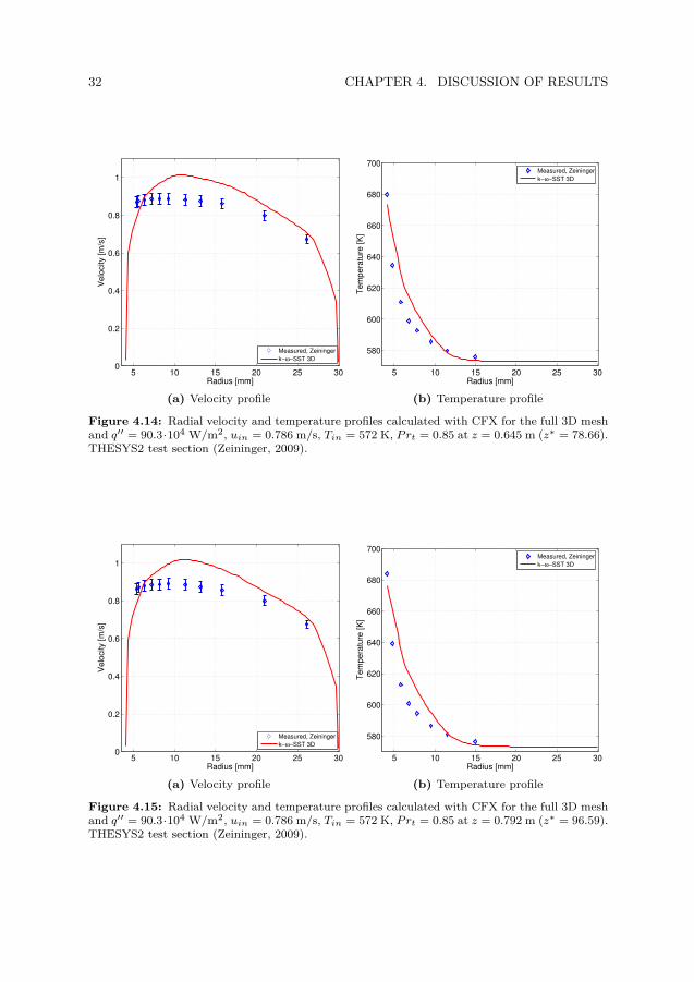
32 CHAPTER 4. DISCUSSION OF RESULTS
5 10 15 20 25 300
0.2
0.4
0.6
0.8
1
Radius [mm]
Ve
locity [
m/s
]
Measured, Zeininger
k−ω−SST 3D
(a) Velocity profile
5 10 15 20 25 30
580
600
620
640
660
680
700
Radius [mm]
Te
mp
era
ture
[K
]
Measured, Zeininger
k−ω−SST 3D
(b) Temperature profile
Figure 4.14: Radial velocity and temperature profiles calculated with CFX for the full 3D meshand q′′ = 90.3·104 W/m2, uin = 0.786 m/s, Tin = 572 K, Prt = 0.85 at z = 0.645 m (z∗ = 78.66).THESYS2 test section (Zeininger, 2009).
5 10 15 20 25 300
0.2
0.4
0.6
0.8
1
Radius [mm]
Ve
locity [
m/s
]
Measured, Zeininger
k−ω−SST 3D
(a) Velocity profile
5 10 15 20 25 30
580
600
620
640
660
680
700
Radius [mm]
Te
mp
era
ture
[K
]
Measured, Zeininger
k−ω−SST 3D
(b) Temperature profile
Figure 4.15: Radial velocity and temperature profiles calculated with CFX for the full 3D meshand q′′ = 90.3·104 W/m2, uin = 0.786 m/s, Tin = 572 K, Prt = 0.85 at z = 0.792 m (z∗ = 96.59).THESYS2 test section (Zeininger, 2009).
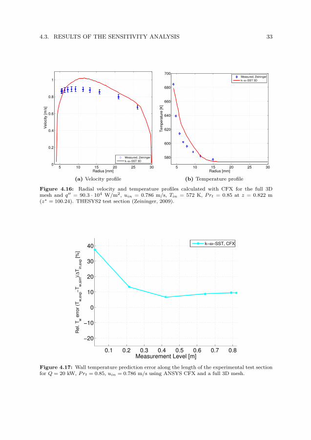
4.3. RESULTS OF THE SENSITIVITY ANALYSIS 33
5 10 15 20 25 300
0.2
0.4
0.6
0.8
1
Radius [mm]
Ve
locity [
m/s
]
Measured, Zeininger
k−ω−SST 3D
(a) Velocity profile
5 10 15 20 25 30
580
600
620
640
660
680
700
Radius [mm]
Te
mp
era
ture
[K
]
Measured, Zeininger
k−ω−SST 3D
(b) Temperature profile
Figure 4.16: Radial velocity and temperature profiles calculated with CFX for the full 3Dmesh and q′′ = 90.3 · 104 W/m2, uin = 0.786 m/s, Tin = 572 K, Prt = 0.85 at z = 0.822 m(z∗ = 100.24). THESYS2 test section (Zeininger, 2009).
0.1 0.2 0.3 0.4 0.5 0.6 0.7 0.8
−20
−10
0
10
20
30
40
Measurement Level [m]
Rel. T
w e
rror
(Tw
,exp−
Tw
,sim
)/∆
Tin
,exp [%
]
k−ω−SST, CFX
Figure 4.17: Wall temperature prediction error along the length of the experimental test sectionfor Q = 20 kW, Prt = 0.85, uin = 0.786 m/s using ANSYS CFX and a full 3D mesh.
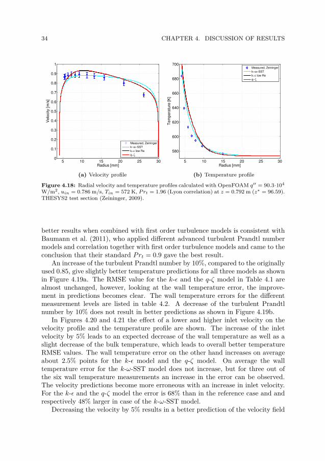
34 CHAPTER 4. DISCUSSION OF RESULTS
5 10 15 20 25 300
0.1
0.2
0.3
0.4
0.5
0.6
0.7
0.8
0.9
1
Radius [mm]
Ve
locity [
m/s
]
Measured, Zeininger
k−ω−SST
k−ε low Re
q−ζ
(a) Velocity profile
5 10 15 20 25 30
580
600
620
640
660
680
700
Radius [mm]T
em
pe
ratu
re [
K]
Measured, Zeininger
k−ω−SST
k−ε low Re
q−ζ
(b) Temperature profile
Figure 4.18: Radial velocity and temperature profiles calculated with OpenFOAM q′′ = 90.3·104
W/m2, uin = 0.786 m/s, Tin = 572 K, Prt = 1.96 (Lyon correlation) at z = 0.792 m (z∗ = 96.59).THESYS2 test section (Zeininger, 2009).
better results when combined with first order turbulence models is consistent withBaumann et al. (2011), who applied different advanced turbulent Prandtl numbermodels and correlation together with first order turbulence models and came to theconclusion that their standard Prt = 0.9 gave the best result.
An increase of the turbulent Prandtl number by 10%, compared to the originallyused 0.85, give slightly better temperature predictions for all three models as shownin Figure 4.19a. The RMSE value for the k-ε and the q-ζ model in Table 4.1 arealmost unchanged, however, looking at the wall temperature error, the improve-ment in predictions becomes clear. The wall temperature errors for the differentmeasurement levels are listed in table 4.2. A decrease of the turbulent Prandtlnumber by 10% does not result in better predictions as shown in Figure 4.19b.
In Figures 4.20 and 4.21 the effect of a lower and higher inlet velocity on thevelocity profile and the temperature profile are shown. The increase of the inletvelocity by 5% leads to an expected decrease of the wall temperature as well as aslight decrease of the bulk temperature, which leads to overall better temperatureRMSE values. The wall temperature error on the other hand increases on averageabout 2.5% points for the k-ε model and the q-ζ model. On average the walltemperature error for the k-ω-SST model does not increase, but for three out ofthe six wall temperature measurements an increase in the error can be observed.The velocity predictions become more erroneous with an increase in inlet velocity.For the k-ε and the q-ζ model the error is 68% than in the reference case and andrespectively 48% larger in case of the k-ω-SST model.
Decreasing the velocity by 5% results in a better prediction of the velocity field
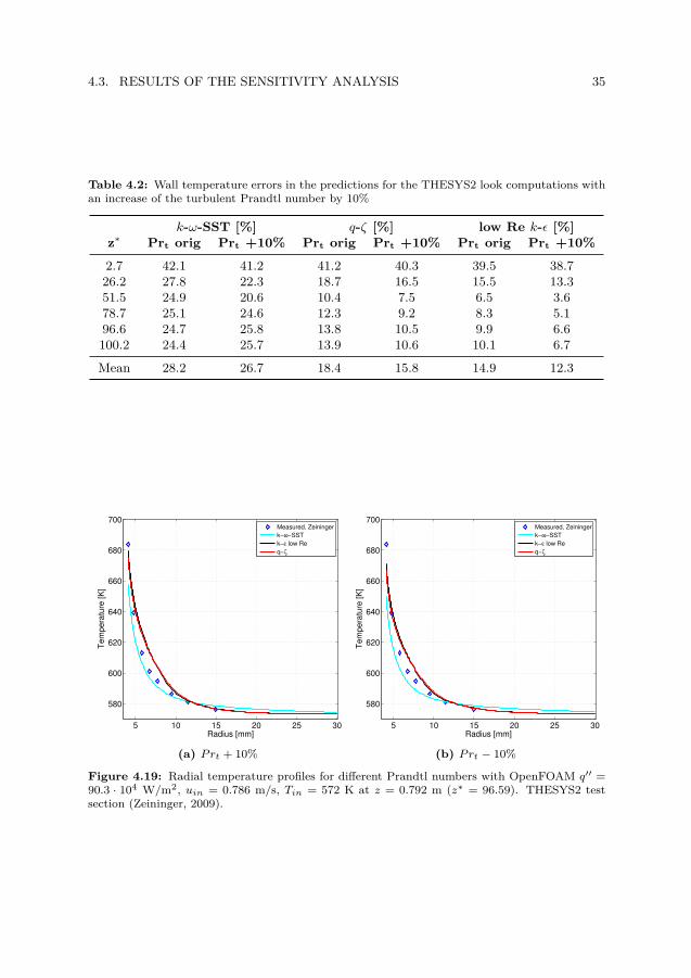
4.3. RESULTS OF THE SENSITIVITY ANALYSIS 35
Table 4.2: Wall temperature errors in the predictions for the THESYS2 look computations withan increase of the turbulent Prandtl number by 10%
k-ω-SST [%] q-ζ [%] low Re k-ε [%]z∗ Prt orig Prt +10% Prt orig Prt +10% Prt orig Prt +10%
2.7 42.1 41.2 41.2 40.3 39.5 38.726.2 27.8 22.3 18.7 16.5 15.5 13.351.5 24.9 20.6 10.4 7.5 6.5 3.678.7 25.1 24.6 12.3 9.2 8.3 5.196.6 24.7 25.8 13.8 10.5 9.9 6.6100.2 24.4 25.7 13.9 10.6 10.1 6.7
Mean 28.2 26.7 18.4 15.8 14.9 12.3
5 10 15 20 25 30
580
600
620
640
660
680
700
Radius [mm]
Te
mp
era
ture
[K
]
Measured, Zeininger
k−ω−SST
k−ε low Re
q−ζ
(a) Prt + 10%
5 10 15 20 25 30
580
600
620
640
660
680
700
Radius [mm]
Te
mp
era
ture
[K
]
Measured, Zeininger
k−ω−SST
k−ε low Re
q−ζ
(b) Prt − 10%
Figure 4.19: Radial temperature profiles for different Prandtl numbers with OpenFOAM q′′ =90.3 · 104 W/m2, uin = 0.786 m/s, Tin = 572 K at z = 0.792 m (z∗ = 96.59). THESYS2 testsection (Zeininger, 2009).
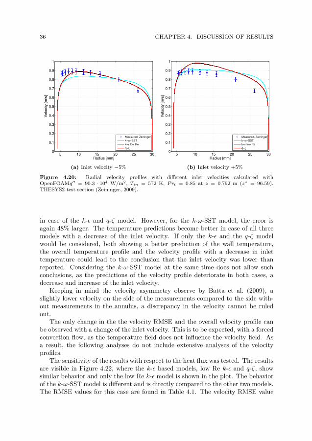
36 CHAPTER 4. DISCUSSION OF RESULTS
5 10 15 20 25 300
0.1
0.2
0.3
0.4
0.5
0.6
0.7
0.8
0.9
1
Radius [mm]
Ve
locity [
m/s
]
Measured, Zeininger
k−ω−SST
k−ε low Re
q−ζ
(a) Inlet velocity −5%
5 10 15 20 25 300
0.1
0.2
0.3
0.4
0.5
0.6
0.7
0.8
0.9
1
Radius [mm]V
elo
city [
m/s
]
Measured, Zeininger
k−ω−SST
k−ε low Re
q−ζ
(b) Inlet velocity +5%
Figure 4.20: Radial velocity profiles with different inlet velocities calculated withOpenFOAMq′′ = 90.3 · 104 W/m2, Tin = 572 K, Prt = 0.85 at z = 0.792 m (z∗ = 96.59).THESYS2 test section (Zeininger, 2009).
in case of the k-ε and q-ζ model. However, for the k-ω-SST model, the error isagain 48% larger. The temperature predictions become better in case of all threemodels with a decrease of the inlet velocity. If only the k-ε and the q-ζ modelwould be considered, both showing a better prediction of the wall temperature,the overall temperature profile and the velocity profile with a decrease in inlettemperature could lead to the conclusion that the inlet velocity was lower thanreported. Considering the k-ω-SST model at the same time does not allow suchconclusions, as the predictions of the velocity profile deteriorate in both cases, adecrease and increase of the inlet velocity.
Keeping in mind the velocity asymmetry observe by Batta et al. (2009), aslightly lower velocity on the side of the measurements compared to the side with-out measurements in the annulus, a discrepancy in the velocity cannot be ruledout.
The only change in the the velocity RMSE and the overall velocity profile canbe observed with a change of the inlet velocity. This is to be expected, with a forcedconvection flow, as the temperature field does not influence the velocity field. Asa result, the following analyses do not include extensive analyses of the velocityprofiles.
The sensitivity of the results with respect to the heat flux was tested. The resultsare visible in Figure 4.22, where the k-ε based models, low Re k-ε and q-ζ, showsimilar behavior and only the low Re k-ε model is shown in the plot. The behaviorof the k-ω-SST model is different and is directly compared to the other two models.The RMSE values for this case are found in Table 4.1. The velocity RMSE value
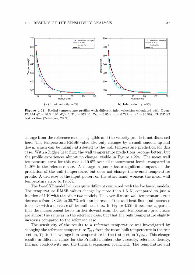
4.3. RESULTS OF THE SENSITIVITY ANALYSIS 37
5 10 15 20 25 30
580
600
620
640
660
680
700
Radius [mm]
Te
mp
era
ture
[K
]
Measured, Zeininger
k−ω−SST
k−ε low Re
q−ζ
(a) Inlet velocity −5%
5 10 15 20 25 30
580
600
620
640
660
680
700
Radius [mm]T
em
pe
ratu
re [
K]
Measured, Zeininger
k−ω−SST
k−ε low Re
q−ζ
(b) Inlet velocity +5%
Figure 4.21: Radial temperature profiles with different inlet velocities calculated with Open-FOAM q′′ = 90.3 · 104 W/m2, Tin = 572 K, Prt = 0.85 at z = 0.792 m (z∗ = 96.59). THESYS2test section (Zeininger, 2009).
change from the reference case is negligible and the velocity profile is not discussedhere. The temperature RMSE value also only changes by a small amount up anddown, which can be mainly attributed to the wall temperature prediction for thiscase. With a higher heat flux, the wall temperature predictions become better, butthe profile experiences almost no change, visible in Figure 4.22a. The mean walltemperature error for this case is 10.6% over all measurement levels, compared to14.9% in the reference case. A change in power has a significant impact on theprediction of the wall temperature, but does not change the overall temperatureprofile. A decrease of the input power, on the other hand, worsens the mean walltemperature error to 19.5%.
The k-ω-SST model behaves quite different compared with the k-ε based models.The temperature RMSE values change by more than 1.5 K, compared to just afraction of 1 K with the other two models. The overall mean wall temperature errordecreases from 28.2% to 25.7% with an increase of the wall heat flux, and increasesto 33.3% with a decrease of the wall heat flux. In Figure 4.22b it becomes apparentthat the measurement levels further downstream, the wall temperature predictionsare almost the same as in the reference case, but that the bulk temperature slightlyincreases compared to the reference case.
The sensitivity of the results to a reference temperature was investigated bychanging the reference temperature Tref from the mean bulk temperature in the testsection, Tb, to the average film temperature in the test section Tfilm. This changeresults in different values for the Prandtl number, the viscosity, reference density,thermal conductivity and the thermal expansion coefficient. The temperature and
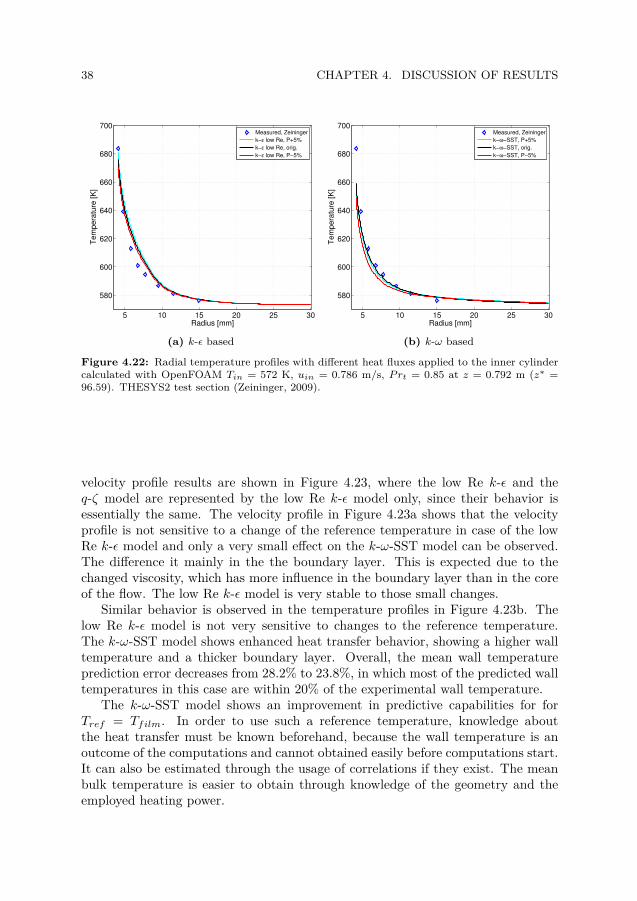
38 CHAPTER 4. DISCUSSION OF RESULTS
5 10 15 20 25 30
580
600
620
640
660
680
700
Radius [mm]
Te
mp
era
ture
[K
]
Measured, Zeininger
k−ε low Re, P+5%
k−ε low Re, orig.
k−ε low Re, P−5%
(a) k-ε based
5 10 15 20 25 30
580
600
620
640
660
680
700
Radius [mm]T
em
pe
ratu
re [
K]
Measured, Zeininger
k−ω−SST, P+5%
k−ω−SST, orig.
k−ω−SST, P−5%
(b) k-ω based
Figure 4.22: Radial temperature profiles with different heat fluxes applied to the inner cylindercalculated with OpenFOAM Tin = 572 K, uin = 0.786 m/s, Prt = 0.85 at z = 0.792 m (z∗ =96.59). THESYS2 test section (Zeininger, 2009).
velocity profile results are shown in Figure 4.23, where the low Re k-ε and theq-ζ model are represented by the low Re k-ε model only, since their behavior isessentially the same. The velocity profile in Figure 4.23a shows that the velocityprofile is not sensitive to a change of the reference temperature in case of the lowRe k-ε model and only a very small effect on the k-ω-SST model can be observed.The difference it mainly in the the boundary layer. This is expected due to thechanged viscosity, which has more influence in the boundary layer than in the coreof the flow. The low Re k-ε model is very stable to those small changes.
Similar behavior is observed in the temperature profiles in Figure 4.23b. Thelow Re k-ε model is not very sensitive to changes to the reference temperature.The k-ω-SST model shows enhanced heat transfer behavior, showing a higher walltemperature and a thicker boundary layer. Overall, the mean wall temperatureprediction error decreases from 28.2% to 23.8%, in which most of the predicted walltemperatures in this case are within 20% of the experimental wall temperature.
The k-ω-SST model shows an improvement in predictive capabilities for forTref = Tfilm. In order to use such a reference temperature, knowledge aboutthe heat transfer must be known beforehand, because the wall temperature is anoutcome of the computations and cannot obtained easily before computations start.It can also be estimated through the usage of correlations if they exist. The meanbulk temperature is easier to obtain through knowledge of the geometry and theemployed heating power.
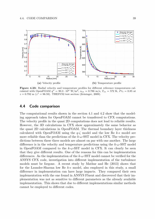
4.4. CODE COMPARISON 39
5 10 15 20 25 300
0.1
0.2
0.3
0.4
0.5
0.6
0.7
0.8
0.9
1
Radius [mm]
Ve
locity [
m/s
]
Measured, Zeiningerk−ε low Re, T
ref=T
bulk
k−ε low Re, Tref
=Tfilm
k−ω−SST, Tref
=Tbulk
k−ω−SST, Tref
=Tfilm
(a) Velocity profile
5 10 15 20 25 30
580
600
620
640
660
680
700
Radius [mm]T
em
pe
ratu
re [
K]
Measured, Zeiningerk−ε low Re, T
ref=T
bulk
k−ε low Re, Tref
=Tfilm
k−ω−SST, Tref
=Tbulk
k−ω−SST, Tref
=Tfilm
(b) Temperature profile
Figure 4.23: Radial velocity and temperature profiles for different reference temperatures cal-culated with OpenFOAM q′′ = 90.3 · 104 W/m2, uin = 0.786 m/s, Tin = 572 K, Prt = 0.85 atz = 0.792 m (z∗ = 96.59). THESYS2 test section (Zeininger, 2009).
4.4 Code comparison
The computational results shown in the section 4.1 and 4.2 show that the model-ing approach taken for OpenFOAM cannot be transferred to CFX computations.The velocity profile in the quasi 2D computations does not lead to reliable results.However, the 3D calculations in CFX show approximately the same behavior asthe quasi 2D calculations in OpenFOAM. The thermal boundary layer thicknesscalculated with OpenFOAM using the q-ζ model and the low Re k-ε model aremore reliable than the predictions of the k-ω-SST model in CFX. The velocity pre-dictions between these three models are almost on par with one another. The largedifference is in the velocity and temperature predictions using the k-ω-SST modelin OpenFOAM compared to the k-ω-SST model in CFX. It can clearly be seenthat they give different results. One of the reasons for this can be implementationdifferences. As the implementation of the k-ω-SST model cannot be verified for theANSYS CFX code, investigation into different implementation of the turbulencemodels must be forgone. A recent study by Mathur and He (2013) shows thatfor the Launder-Sharma low Re k-ε model, also employed in this study, a smalldifference in implementation can have large impacts. They compared their ownimplementation with the one found in ANSYS Fluent and discovered that their im-plementation was not as sensitive to different parameters as the already availableimplementation. This shows that due to different implementations similar methodscannot be employed to different codes.

Chapter 5
Conclusions and Future Work
In this study forced convection of LBE was studied. Two different codes, Open-FOAM and CFX, were used to compute the velocity and temperature field of theTHESYS2 experiment, whereas only OpenFOAM was used in computations per-taining the TALL experiment. Three different turbulence models in OpenFOAMand one turbulence model in CFX were tested.
The computations show that RANS turbulence models are generally capable togive sufficient results to such computations. The direct comparison between thetwo codes shows that modeling approaches which are valid for one code cannotdirectly applied to a different code without modification. In this case CFX is notcapable of predicting the velocity profiles in a quasi 2D modeling setup, in whichOpenFOAM gives sufficient results compared to the experimental data.
In case of OpenFOAM, the low Re k-ε model and the q-ζ model show similarsensitivity to the selection of the turbulent Prandtl number, Prt, and other param-eters, which results from the similarity in formulation of the two models. A strongsensitivity to the selection of the turbulent Prandtl number can be observed. Inparticular, a slight increase of the turbulent Prandtl number from 0.85, which wasused in the reference case, leads to an improvement in the temperature predictions,especially in the predictions of the wall temperature. A slight decrease however,can lead to a deterioration of the temperature predictions, all while the velocitypredictions are unaffected. The current study also shows that an advanced tur-bulent Prandtl number correlation does not necessarily lead to better prediction.The Lyon based turbulent Prandtl number correlation leads to bad results in allthree tested models. This is consistent with Baumann et al. (2011), who compareddifferent advanced turbulent Prandtl number correlations in combination with firstorder turbulence models, but obtained the best results with a constant turbulentPrandtl number of 0.9.
As previously mentioned, the velocity profile was not affected by changes toparameters determining the heat transfer, which was expected, as there is only aweak influence on the momentum equations by the temperature field through the
41
42 CHAPTER 5. CONCLUSIONS AND FUTURE WORK
Boussinesq approximation for buoyancy. It makes this modeling approach suitablefor calculations of forced convection flows. The magnitude of the inlet velocity isthe only strong influence on the velocity field prediction which was observed. Fromthe CFX cases it also becomes apparent that a high quality inlet velocity profile isof importance for the predictions.
The studies modeling approach, including the selected turbulence models anda fixed Prandtl number, should only be used for forced convection only. In thecase of mixed and natural convection, phenomena such as turbulence production bybuoyancy, are added to the complexity and the models that are employed for forcedconvection cannot account for such phenomena. The presented research showedthat the choice of the turbulent Prandtl number in dependence of the turbulencemodel plays a role in the predictive capabilities of the model itself. Therefore,further research should be conducted to find out which combination of turbulentPrandtl number and turbulence model are suitable for which range of flows in orderto assess the suitability of the present tools to liquid metal flows.
The computations with CFX showed that there is a strong dependence on themodeling method. It should therefore be investigated if the OpenFOAM predictioncan benefit from a full 3D modeling approach similar to the one taken in CFX.Furthermore, a full investigation of the 3D case in CFX will follow, determiningthe sensitivity of the modeling approach so modeling parameters and boundaryconditions. This will contribute to a better assessment and comparison of the twocodes at hand.
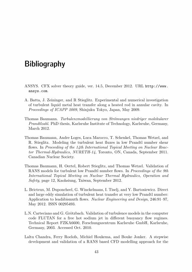
Bibliography
ANSYS. CFX solver theory guide, ver. 14.5, December 2012. URL http://www.ansys.com.
A. Batta, J. Zeininger, and R Stieglitz. Experimental and numerical investigationof turbulent liquid metal heat transfer along a heated rod in annular cavity. InProceedings of ICAPP 2009, Shinjuku Tokyo, Japan, May 2009.
Thomas Baumann. Turbulenzmodellierung von Strömungen niedriger molekularerPrandtlzahl. PhD thesis, Karlsruhe Institute of Technology, Karlsruhe, Germany,March 2012.
Thomas Baumann, Andre Loges, Luca Marocco, T. Schenkel, Thomas Wetzel, andR. Stieglitz. Modeling the turbulent heat fluxes in low Prandtl number shearflows. In Proceeding of the 14th International Topical Meeting on Nuclear Reac-tor Thermal-Hydraulics, NURETH-14, Toronto, ON, Canada, September 2011.Canadian Nuclear Society.
Thomas Baumann, H. Oertel, Robert Stieglitz, and Thomas Wetzel. Validation ofRANS models for turbulent low Prandtl number flows. In Proceedings of the 9thInternational Topical Meeting on Nuclear Thermal Hydraulics, Operation andSafety, page 12, Kaohsiung, Taiwan, September 2012.
L. Bricteux, M. Duponcheel, G. Winckelmans, I. Tiselj, and Y. Bartosiewicz. Directand large eddy simulation of turbulent heat transfer at very low Prandtl number:Application to leadâbismuth flows. Nuclear Engineering and Design, 246:91–97,May 2012. ISSN 00295493.
L.N. Carteciano and G. Grötzbach. Validation of turbulence models in the computercode FLUTAN for a free hot sodium jet in different buoyancy flow regimes.Technical Report FZKA6600, Forschungszentrum Karlsruhe GmbH, Karlsruhe,Germany, 2003. Accessed Oct. 2010.
Laltu Chandra, Ferry Roelofs, Michiel Houkema, and Bouke Jonker. A stepwisedevelopment and validation of a RANS based CFD modelling approach for the
43
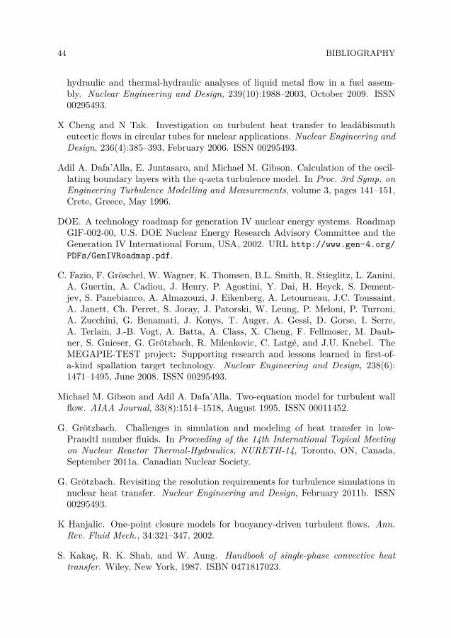
44 BIBLIOGRAPHY
hydraulic and thermal-hydraulic analyses of liquid metal flow in a fuel assem-bly. Nuclear Engineering and Design, 239(10):1988–2003, October 2009. ISSN00295493.
X Cheng and N Tak. Investigation on turbulent heat transfer to leadâbismutheutectic flows in circular tubes for nuclear applications. Nuclear Engineering andDesign, 236(4):385–393, February 2006. ISSN 00295493.
Adil A. Dafa’Alla, E. Juntasaro, and Michael M. Gibson. Calculation of the oscil-lating boundary layers with the q-zeta turbulence model. In Proc. 3rd Symp. onEngineering Turbulence Modelling and Measurements, volume 3, pages 141–151,Crete, Greece, May 1996.
DOE. A technology roadmap for generation IV nuclear energy systems. RoadmapGIF-002-00, U.S. DOE Nuclear Energy Research Advisory Committee and theGeneration IV International Forum, USA, 2002. URL http://www.gen-4.org/PDFs/GenIVRoadmap.pdf.
C. Fazio, F. Gröschel, W. Wagner, K. Thomsen, B.L. Smith, R. Stieglitz, L. Zanini,A. Guertin, A. Cadiou, J. Henry, P. Agostini, Y. Dai, H. Heyck, S. Dement-jev, S. Panebianco, A. Almazouzi, J. Eikenberg, A. Letourneau, J.C. Toussaint,A. Janett, Ch. Perret, S. Joray, J. Patorski, W. Leung, P. Meloni, P. Turroni,A. Zucchini, G. Benamati, J. Konys, T. Auger, A. Gessi, D. Gorse, I. Serre,A. Terlain, J.-B. Vogt, A. Batta, A. Class, X. Cheng, F. Fellmoser, M. Daub-ner, S. Gnieser, G. Grötzbach, R. Milenkovic, C. Latgé, and J.U. Knebel. TheMEGAPIE-TEST project: Supporting research and lessons learned in first-of-a-kind spallation target technology. Nuclear Engineering and Design, 238(6):1471–1495, June 2008. ISSN 00295493.
Michael M. Gibson and Adil A. Dafa’Alla. Two-equation model for turbulent wallflow. AIAA Journal, 33(8):1514–1518, August 1995. ISSN 00011452.
G. Grötzbach. Challenges in simulation and modeling of heat transfer in low-Prandtl number fluids. In Proceeding of the 14th International Topical Meetingon Nuclear Reactor Thermal-Hydraulics, NURETH-14, Toronto, ON, Canada,September 2011a. Canadian Nuclear Society.
G. Grötzbach. Revisiting the resolution requirements for turbulence simulations innuclear heat transfer. Nuclear Engineering and Design, February 2011b. ISSN00295493.
K Hanjalic. One-point closure models for buoyancy-driven turbulent flows. Ann.Rev. Fluid Mech., 34:321–347, 2002.
S. Kakaç, R. K. Shah, and W. Aung. Handbook of single-phase convective heattransfer. Wiley, New York, 1987. ISBN 0471817023.
BIBLIOGRAPHY 45
Hiroshi Kawamura, Hiroyuki Abe, and Yuichi Matsuo. DNS of turbulent heattransfer in channel flow with respect to Reynolds and Prandtl number effects.International Journal of Heat and Fluid Flow, 20(3):196–207, June 1999. ISSN0142727X.
LBE Handbook. Handbook on lead-bismuth eutectic alloy and lead properties,materials compatibility, thermal-hydraulics and technologies. OECD NuclearEnergy Agency, Issy-les-Moulineaux France, 2007 ed. edition, 2007. ISBN9789264990029.
André Loges. Untersuchungen zum turbulenten Wärmeübergang im flüssigmetall-durchströmten konzentrischen Ringspalt. Master thesis, Karlsruhe Institute ofTechnology, Karlsruhe, Germany, November 2010.
Weimin Ma, Aram Karbojian, Thorsten Hollands, and Marco K. Koch. Experimen-tal and numerical study on lead-bismuth heat transfer in a fuel rod simulator.Journal of Nuclear Materials, April 2011. ISSN 00223115.
Luca Marocco, André Loges, Thomas Wetzel, and Robert Stieglitz. Experimen-tal investigation of the turbulent heavy liquid metal heat transfer in the thermalentry region of a vertical annulus with constant heat flux on the inner surface. In-ternational Journal of Heat and Mass Transfer, 55(23-24):6435–6445, November2012. ISSN 00179310.
A. Mathur and S. He. Performance and Implementation of the Launder-SharmaLow-Reynolds Number Turbulence Model. Computers & Fluids, March 2013.ISSN 00457930.
F. R. Menter. Two-equation eddy-viscosity turbulence models for engineering ap-plications. AIAA Journal, 32(8):1598–1605, August 1994. ISSN 0001-1452.
K. Natesan, T. Sundararajan, Arunn Narasimhan, and K. Velusamy. Turbulentflow simulation in a wire-wrap rod bundle of an LMFBR. Nuclear Engineeringand Design, 240(5):1063–1072, May 2010. ISSN 00295493.
OpenCFD Ltd (ESI Group). OpenFOAM programmer’s C++ documentation,2011. URL http://foam.sourceforge.net/doc/Doxygen/html/. retrieved Sep14, 2011, Published by OpenCFD Limited.
OpenFOAM. OpenFOAM programmer’s C++ documentation, March 2013. URLhttp://www.openfoam.org/docs/cpp/.
M. Ould-Rouiss, L. Redjem-Saad, G. Lauriat, and A. Mazouz. Effect of Prandtlnumber on the turbulent thermal field in annular pipe flow. International Com-munications in Heat and Mass Transfer, 37(8):958–963, October 2010. ISSN07351933.
46 BIBLIOGRAPHY
Marco Pellegrini, Hiroshi Endo, and Hisashi Ninokata. Algebraic turbulent heat fluxmodel for prediction of thermal stratification in piping systems. In Proceeding ofthe 14th International Topical Meeting on Nuclear Reactor Thermal-Hydraulics,NURETH-14, Toronto, ON, Canada, September 2011. Canadian Nuclear Society.
F. Roelofs, M. Rohde, I. Otić, G. Brillant, I. Tiselj, H. Anglart, B. Niceno,L. Bricteux, D. Angeli, W. Ambrosini, D. Lakehal, E. Baglietto, Y. Hassan, andX. Cheng. European developments in single phase turbulence for innovative reac-tors. In Proceeding of the 14th International Topical Meeting on Nuclear ReactorThermal-Hydraulics, NURETH-14, volume 1, Toronto, ON, Canada, September2011. Canadian Nuclear Society.
Hermann Schlichting and K. Gersten. Boundary-layer theory. Springer, Berlin ;New York, 8th rev. and enl. ed edition, 2000. ISBN 3540662707.
Roman Thiele and Henryk Anglart. Numerical modeling of forced-convection heattransfer to lead-bismuth eutectic flowing in vertical annuli. Nuclear Engineeringand Design, 254:111–119, January 2013. ISSN 00295493.
Roman Thiele, Weimin Ma, and Henryk Anglart. Investigation of the influenceof turbulence models on the prediction of heat transfer to low Prandtl numberfluids. In Proceeding of the 14th International Topical Meeting on Nuclear Reac-tor Thermal-Hydraulics, NURETH-14, Toronto, ON, Canada, September 2011.Canadian Nuclear Society.
Janne Wallenius, Erdenechimeg Suvdantsetseg, and Andrei Fokau. ELECTRA:European Lead-Cooled Training Reactor. Nuclear Technology, 177(3):303–313,March 2012.
David Wilcox. Turbulence modeling for CFD. DCW Industries, La Cañada Calif.,3rd edition, 2006. ISBN 9781928729082.
Jörg Zeininger. Turbulenter Wärmetransport in flüssigem Blei-Wismut an einemvertikalen Heizstab im Ringspalt. PhD thesis, Karlsruhe Institute of Technology,Karlsruhe, Germany, March 2009.