0

Prospectus of

“Framework for creating large-scale content-based image retrieval system (CBIR)

for solar data analysis”

Juan M. Banda

1

Outline

1. Project Summary ………………………………………………………………………………………… 2

2. Project Overview ………………………………………………………………………………………… 3

2.1. Objectives and Expected Significance

2.1.1. Creation of a CBIR building framework

2.1.1.1. Creation of a composite multi-dimensional indexing technique

2.1.2. Creation of a CBIR for Solar Dynamics Observatory

2.2. Research Description ……………………………………………………………………….... 4

2.3. Datasets to analyze …………………………………………………………………………... 8

2.3.1. TRACE Dataset

2.3.2. INDECS Database

2.3.3. ImageCLEFmed Dataset

2.4. Deliverables …………………………………………………………………………………. 11

3. Background information ………………………………………………………………………………... 12

3.1. Activity in the solar community

3.2. Image descriptors/parameters

3.3. Unsupervised Attribute Evaluation

3.4. Supervised Attribute Evaluation

3.5. Dissimilarity Measures (Euclidean distance, Standardized Euclidean distance, Mahalanobis

distance, City block distance, Chebychev distance, Cosine distance, Correlation distance,

Spearman distance, Hausdorff Distance, Jensen–Shannon divergence (JSD), χ2 distance,

Kullback–Leibler divergence (KLD))

3.6. Dimensionality reduction

3.6.1. Linear dimensionality reduction methods (Principal Component Analysis (PCA),

Singular Value Decomposition (SVD), Locality Preserving Projections (LPP), Factor

Analysis (FA))

3.6.2. Non-linear dimensionality reduction methods (Kernel PCA, Isomap, Locally-

Linear Embedding (LLE), Laplacian Eigenmaps (LE))

3.7. Indexing techniques

3.7.1. Single-Dimensional Indexing for Multi-Dimensional Data (iDistance, iMinMax,

UB-Trees, Pyramid-trees)

3.7.2. Multi-Dimensional Indexing (R+-Trees, R*-Trees, TV-trees, X-trees)

References ………………………………………………………………………………………………… 26

2

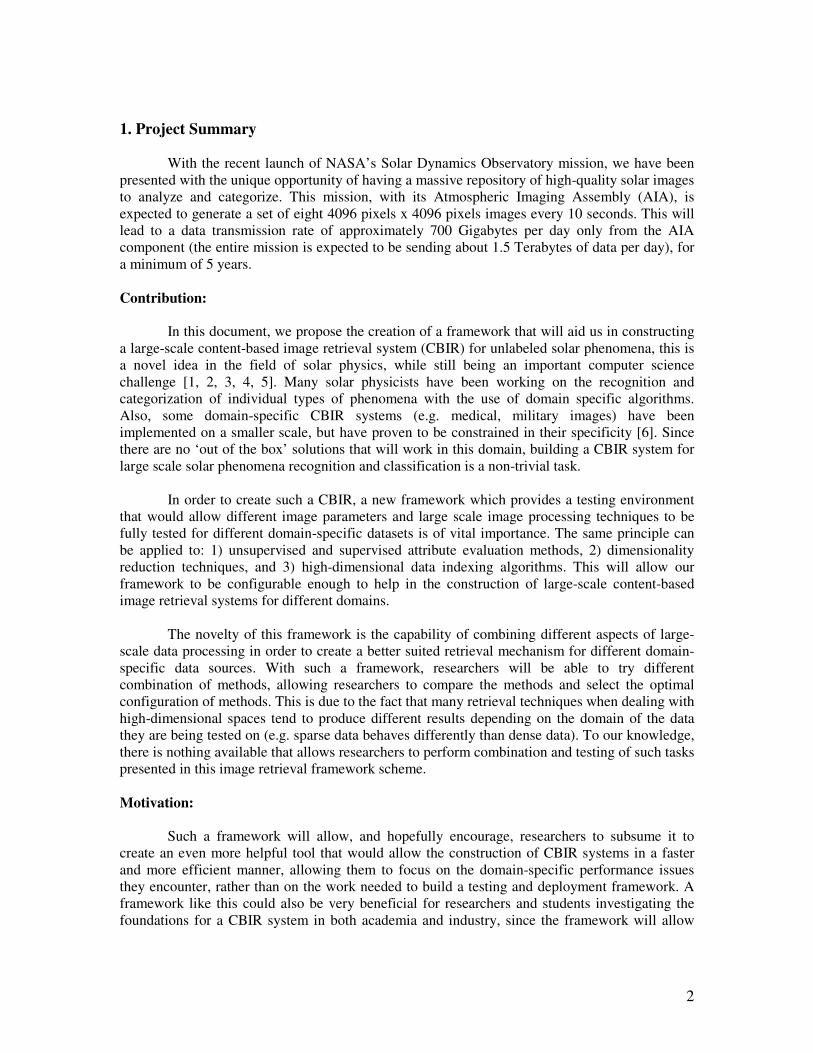
1. Project Summary

With the recent launch of NASA’s Solar Dynamics Observatory mission, we have been

presented with the unique opportunity of having a massive repository of high-quality solar images

to analyze and categorize. This mission, with its Atmospheric Imaging Assembly (AIA), is

expected to generate a set of eight 4096 pixels x 4096 pixels images every 10 seconds. This will

lead to a data transmission rate of approximately 700 Gigabytes per day only from the AIA

component (the entire mission is expected to be sending about 1.5 Terabytes of data per day), for

a minimum of 5 years.

Contribution:

In this document, we propose the creation of a framework that will aid us in constructing

a large-scale content-based image retrieval system (CBIR) for unlabeled solar phenomena, this is

a novel idea in the field of solar physics, while still being an important computer science

challenge [1, 2, 3, 4, 5]. Many solar physicists have been working on the recognition and

categorization of individual types of phenomena with the use of domain specific algorithms.

Also, some domain-specific CBIR systems (e.g. medical, military images) have been

implemented on a smaller scale, but have proven to be constrained in their specificity [6]. Since

there are no ‘out of the box’ solutions that will work in this domain, building a CBIR system for

large scale solar phenomena recognition and classification is a non-trivial task.

In order to create such a CBIR, a new framework which provides a testing environment

that would allow different image parameters and large scale image processing techniques to be

fully tested for different domain-specific datasets is of vital importance. The same principle can

be applied to: 1) unsupervised and supervised attribute evaluation methods, 2) dimensionality

reduction techniques, and 3) high-dimensional data indexing algorithms. This will allow our

framework to be configurable enough to help in the construction of large-scale content-based

image retrieval systems for different domains.

The novelty of this framework is the capability of combining different aspects of large-

scale data processing in order to create a better suited retrieval mechanism for different domain-

specific data sources. With such a framework, researchers will be able to try different

combination of methods, allowing researchers to compare the methods and select the optimal

configuration of methods. This is due to the fact that many retrieval techniques when dealing with

high-dimensional spaces tend to produce different results depending on the domain of the data

they are being tested on (e.g. sparse data behaves differently than dense data). To our knowledge,

there is nothing available that allows researchers to perform combination and testing of such tasks

presented in this image retrieval framework scheme.

Motivation:

Such a framework will allow, and hopefully encourage, researchers to subsume it to

create an even more helpful tool that would allow the construction of CBIR systems in a faster

and more efficient manner, allowing them to focus on the domain-specific performance issues

they encounter, rather than on the work needed to build a testing and deployment framework. A

framework like this could also be very beneficial for researchers and students investigating the

foundations for a CBIR system in both academia and industry, since the framework will allow

3

them to quickly test predetermined image parameters, image processing techniques, etc. in their

own domain specific dataset without the need of starting from scratch.

2. Project Description

2.1. Objectives and Expected Significance

2.1.1. Creation of a CBIR building framework

With our novel application came the realization that while most stages and techniques

needed to develop a CBIR are available via countless research papers, survey papers, algorithm

implementations, and open source CBIR systems. There is the lack of a common framework that

would allow researchers to fully focus on the peculiarity of their domain-specific image dataset

rather than building a testing environment, gathering code from multiple sources and

implementing everything in order to be able to test new image parameters on their specific image

dataset. With such a big missing component, and based on our own experience, we theorize that

many researchers in this area are spending most of their time building their testing framework and

adding features to it, rather than testing the image parameters they desire and focusing on how to

better describe their images in terms of building an image parameter vector.

We believe this is a considerable contribution since it will allow future researchers to

spend their time in other sections that will allow their CBIR system to be more optimized for their

domain-specific task. With all the components of this framework our work in creating a CBIR

system for the Solar Dynamics Observatory has been greatly aided in terms of being able to test

new image parameters, dimensionality reduction methods, etc. seamlessly and allowing us to fine

tune our system for better performance.

2.1.1.1. Creation of a composite multi-dimensional indexing technique

An important addition to our CBIR building framework is the ability to allow the user to

use one of several indexing mechanisms for their image parameter vector. With high-

dimensionality comes high complexity in terms of data retrieval and many of the current high-

dimensional indexing methods rely on a combination of some kind of dimensionality reduction

method and translating the new dimensional space into 1-D segments to be efficiently indexed by

a B+-tree. In our framework the user will be able to select one of our eight state-of-the-art

dimensionality reduction methods and combine (and test) them with eight different high-

dimensional data indexing mechanisms. This will allow users to test and select the most optimal

retrieval mechanism for their needs. Since most retrieval mechanisms are highly domain-

dependent, here users can test several indexing mechanism combinations and pick the best, or

they can implement their own which can be added in the future to this framework.

2.1.2. Creation of a CBIR for Solar Dynamics Observatory

The need to quickly identify the growing number of solar images provided by the Solar

Dynamics Observatory is of great importance since with the volume of data generated, timely

hand-labeling is simply impossible. Individual algorithms work on identifying particular solar

phenomena in SDO images, but they are not fully integrated to allow researches to query their

4

entire repositories, let alone in a combination of them. In our novel approach, our goal is to have

at least ten different solar phenomena classes in our CBIR system (currently we have eight),

allowing scientists to quickly retrieve similar images to the ones they find more interesting, and

search in a repository that contains more than one type of solar phenomenon.

2.2. Research Description

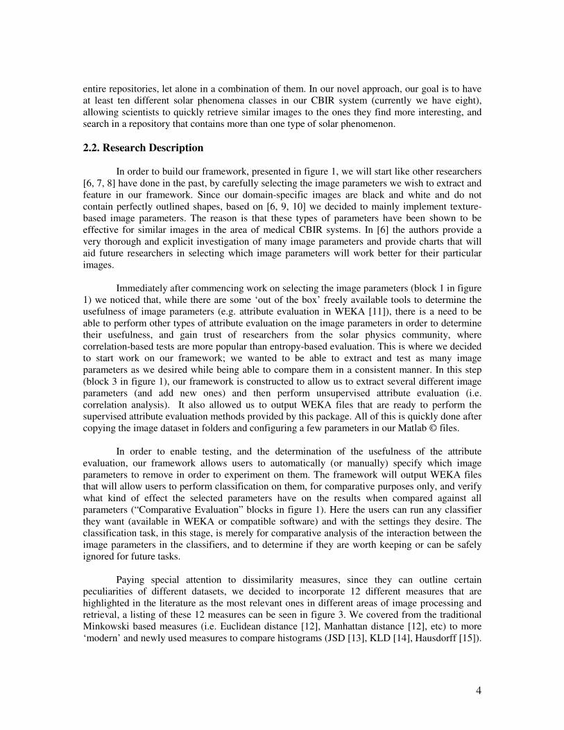
In order to build our framework, presented in figure 1, we will start like other researchers

[6, 7, 8] have done in the past, by carefully selecting the image parameters we wish to extract and

feature in our framework. Since our domain-specific images are black and white and do not

contain perfectly outlined shapes, based on [6, 9, 10] we decided to mainly implement texture-

based image parameters. The reason is that these types of parameters have been shown to be

effective for similar images in the area of medical CBIR systems. In [6] the authors provide a

very thorough and explicit investigation of many image parameters and provide charts that will

aid future researchers in selecting which image parameters will work better for their particular

images.

Immediately after commencing work on selecting the image parameters (block 1 in figure

1) we noticed that, while there are some ‘out of the box’ freely available tools to determine the

usefulness of image parameters (e.g. attribute evaluation in WEKA [11]), there is a need to be

able to perform other types of attribute evaluation on the image parameters in order to determine

their usefulness, and gain trust of researchers from the solar physics community, where

correlation-based tests are more popular than entropy-based evaluation. This is where we decided

to start work on our framework; we wanted to be able to extract and test as many image

parameters as we desired while being able to compare them in a consistent manner. In this step

(block 3 in figure 1), our framework is constructed to allow us to extract several different image

parameters (and add new ones) and then perform unsupervised attribute evaluation (i.e.

correlation analysis). It also allowed us to output WEKA files that are ready to perform the

supervised attribute evaluation methods provided by this package. All of this is quickly done after

copying the image dataset in folders and configuring a few parameters in our Matlab © files.

In order to enable testing, and the determination of the usefulness of the attribute

evaluation, our framework allows users to automatically (or manually) specify which image

parameters to remove in order to experiment on them. The framework will output WEKA files

that will allow users to perform classification on them, for comparative purposes only, and verify

what kind of effect the selected parameters have on the results when compared against all

parameters (“Comparative Evaluation” blocks in figure 1). Here the users can run any classifier

they want (available in WEKA or compatible software) and with the settings they desire. The

classification task, in this stage, is merely for comparative analysis of the interaction between the

image parameters in the classifiers, and to determine if they are worth keeping or can be safely

ignored for future tasks.

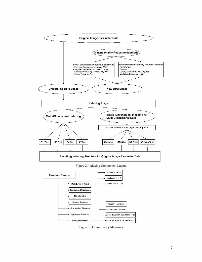
Paying special attention to dissimilarity measures, since they can outline certain

peculiarities of different datasets, we decided to incorporate 12 different measures that are

highlighted in the literature as the most relevant ones in different areas of image processing and

retrieval, a listing of these 12 measures can be seen in figure 3. We covered from the traditional

Minkowski based measures (i.e. Euclidean distance [12], Manhattan distance [12], etc) to more

‘modern’ and newly used measures to compare histograms (JSD [13], KLD [14], Hausdorff [15]).

5

With the addition of these measures, we allow future users of our framework to test different

measures that will allow them to gain different insights on their domain-specific datasets when

performing correlation analysis on their datasets. These measures will also be of great use for our

multi-dimensional indexing component of the framework as well, and will be discussed again in

later in this section.

One of the most important stages in building a CBIR system and in our framework is the

dimensionality reduction stage (see block 4 in figure 1). Since most image parameter vectors are

very high in dimensionality, they will become very problematic when it is time to store, query

and retrieve them depending on the volume of the dataset. We have incorporated in our

framework eight different dimensionality reduction techniques that will allow the researcher to

determine which of them produces the best (or closest to the best) results in their domain-specific

dataset. Since most datasets are different, we incorporated different linear and non-linear

dimensionality reduction techniques that take advantage of different properties of the dataset in

order to produce an optimal low-dimensional representation of the original data. These techniques

vary from the classical Principal Component Analysis [16] to more modern methods like

Laplacian Eigen maps [17], and Locally-Linear Embedding [18] among others, with the only

common factor that all of these methods employed in our framework have a mapping function to

map new unseen data into the produced artificial dimensional spaces. Having a mapping function

is a fundamentally important issue since we want to be able to use these mapping functions to

process new/unseen data from the user’s queries.

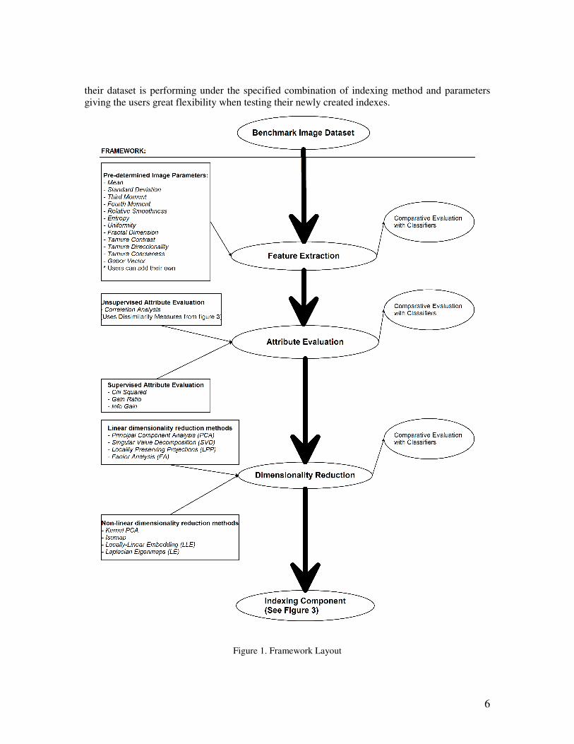
In the last section of our framework (see block 5 in figure 1, and figure 2) we tackle the

problem of indexing multi-dimensional data by providing the user with eight different indexing

mechanisms to try on their datasets. With an innovative and configurable set-up, we will allow

users to combine all the previously mentioned similarity measures and dimensionality reduction

methods alongside with several of the indexing mechanisms, in order to produce domain-specific

indexing structures. There have been plenty of differently named indexing mechanisms that allow

users to use different similarity measures and dimensionality reduction techniques in order to

achieve efficient retrieval, but only for a few domain specific problems [19, 20, 21]. Our

framework has more of a ‘plug and play’ feel to it, since the users are not restricted in any

combination of measures (figure 3) / dimensionality reduction techniques (figure 2) that they

wants to investigate. The user can also add the ones he desires and use our mechanism to combine

them.

As outlined in this document (and on figure 1), the proposed framework will allow users

to efficiently test image parameters that will be later used on their domain-specific CBIR system.

This framework provides a solid foundation of evaluation methods and experimental evaluation

that is currently not available in any other freely available software. By combining Matlab scripts

and toolboxes, with open source indexing algorithm implementation, and with WEKA’s API we

provide users the ability to quickly interconnect these two software packages and focus more on

the dataset-specific problems they encounter and not on the implementation side of things. Going

a step further, for people with high-dimensional datasets we provide capabilities of testing several

dimensionality reduction methods at once to help them with their dimensionality issue. Since

retrieval is one of the most important parts for the success of CBIR systems, we also include a

module (block 5 in figure 1) that allows users to fine-tune widely accepted multi-dimensional

indexing mechanisms to better fit their needs by allowing them to change a wide variety of

parameters. This module also contains testing facilities that will allow them to easily verify how

6

their dataset is performing under the specified combination of indexing method and parameters

giving the users great flexibility when testing their newly created indexes.

Figure 1. Framework Layout

7

Figure 2. Indexing Component Layout

Figure 3. Dissimilarity Measures

8

2.3. Datasets to be analyzed

In our domain specific problem (solar images) we found that since there was no widely

available multi-class dataset, we had to create our own. Introduced in [22] our dataset covers

several different solar phenomena in equally balanced representations, a detailed description of

this dataset is found in section 2.3.1. For comparison purposes we also analyzed two other

domain specific (and very different datasets) that feature very similar characteristics in terms of

image size and class balancing, which we will discus in sections 2.3.2 and 2.3.3.

2.3.1. TRACE Dataset

The TRACE dataset was created using the Heliophysics Events Knowledgebase (HEK)

portal [23] to find the event dates. Then we retrieved the actual images using the TRACE Data

Analysis Center’s catalog search [24]. The search extends into the TRACE repository as well as

other repositories. To make all images consistent, we filtered out all results that did not came

from the TRACE mission. Table 1 provides an overview of our dataset. All images selected have

an extent label of “Partial Sun”

In the process of creating our dataset to analyze parameters for image recognition we

stumbled upon several problems when trying to balance the number of images per class. First, we

found that several phenomena do not occur as often as others, making it harder to balance the

number of images between individual classes. The second issue is that several phenomena can be

sighted and reported in different wavelengths. For our benchmark we selected the wavelengths

that contained the largest number of hand labeled results provided by HEK contributors. The third

issue we encounter is very inconsistent labeling of phenomena over the course of its duration.

Finally, the images retrieved had different resolutions so we needed experimented the trade-off

(i.e 768x768 to 1024x1024) when re-sizing images and decided to transform them into the same

resolution. Part of the motivation behind this work is to solve these previously mentioned

problems.

All events retrieved were queried within the 99-11-03 to 08-11-04 date ranges. As one can see

from the table 1, for the 16 events searchable by HEK we had to reduce the number of events to 8

due to the limited number of available occurrences of the remaining types of phenomena and poor

quality of images available in some of the data catalogs. The current selection of classes was

solely based on the number of images available, and the wavelengths in which the images where

available. We wanted to be sure that our benchmark data set has equally frequent classes in order

to be sure that our results are not skewed towards the most frequent phenomena. For the events

that occurred only a few times, but during a prolonged period of time, we have selected a few

different images within that time range to complete our goal of 200 images per event class.

Table 1: Characteristics of our benchmark data set

Event Name # of images retrieved Wavelength

Active Region 200 1600

Coronal Jet 200 171

Emerging Flux 200 1600

Filament 200 171

Filament Activation 200 171

Filament Eruption 200 171

Flare 200 171

Oscillation 200 171

9

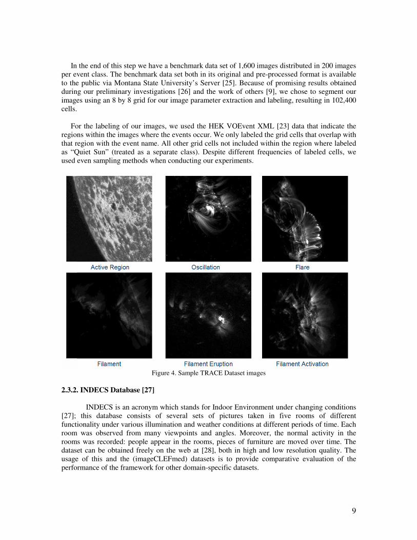
In the end of this step we have a benchmark data set of 1,600 images distributed in 200 images

per event class. The benchmark data set both in its original and pre-processed format is available

to the public via Montana State University’s Server [25]. Because of promising results obtained

during our preliminary investigations [26] and the work of others [9], we chose to segment our

images using an 8 by 8 grid for our image parameter extraction and labeling, resulting in 102,400

cells.

For the labeling of our images, we used the HEK VOEvent XML [23] data that indicate the

regions within the images where the events occur. We only labeled the grid cells that overlap with

that region with the event name. All other grid cells not included within the region where labeled

as “Quiet Sun” (treated as a separate class). Despite different frequencies of labeled cells, we

used even sampling methods when conducting our experiments.

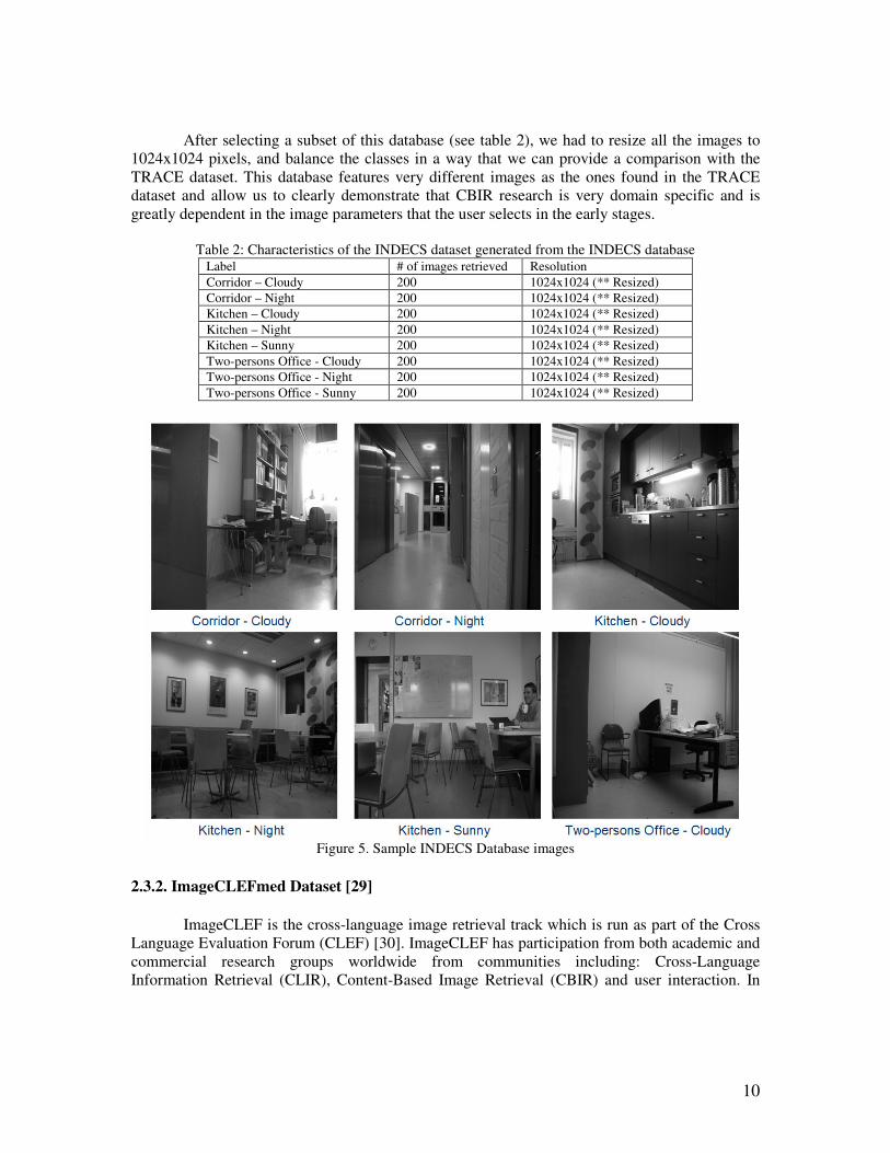
Figure 4. Sample TRACE Dataset images

2.3.2. INDECS Database [27]

INDECS is an acronym which stands for Indoor Environment under changing conditions

[27]; this database consists of several sets of pictures taken in five rooms of different

functionality under various illumination and weather conditions at different periods of time. Each

room was observed from many viewpoints and angles. Moreover, the normal activity in the

rooms was recorded: people appear in the rooms, pieces of furniture are moved over time. The

dataset can be obtained freely on the web at [28], both in high and low resolution quality. The

usage of this and the (imageCLEFmed) datasets is to provide comparative evaluation of the

performance of the framework for other domain-specific datasets.

10

After selecting a subset of this database (see table 2), we had to resize all the images to

1024x1024 pixels, and balance the classes in a way that we can provide a comparison with the

TRACE dataset. This database features very different images as the ones found in the TRACE

dataset and allow us to clearly demonstrate that CBIR research is very domain specific and is

greatly dependent in the image parameters that the user selects in the early stages.

Table 2: Characteristics of the INDECS dataset generated from the INDECS database

Label # of images retrieved Resolution

Corridor – Cloudy 200 1024x1024 (** Resized)

Corridor – Night 200 1024x1024 (** Resized)

Kitchen – Cloudy 200 1024x1024 (** Resized)

Kitchen – Night 200 1024x1024 (** Resized)

Kitchen – Sunny 200 1024x1024 (** Resized)

Two-persons Office - Cloudy 200 1024x1024 (** Resized)

Two-persons Office - Night 200 1024x1024 (** Resized)

Two-persons Office - Sunny 200 1024x1024 (** Resized)

Figure 5. Sample INDECS Database images

2.3.2. ImageCLEFmed Dataset [29]

ImageCLEF is the cross-language image retrieval track which is run as part of the Cross

Language Evaluation Forum (CLEF) [30]. ImageCLEF has participation from both academic and

commercial research groups worldwide from communities including: Cross-Language

Information Retrieval (CLIR), Content-Based Image Retrieval (CBIR) and user interaction. In

11

their medical retrieval task, we find several datasets available: 2005, 2006, 2007, and 2010 (that

features an augmented version of the 2008 and 2009 datasets).

Currently, we just received access to the 2005, 2006 and 2007 datasets. The 2005 dataset

consists of 10,000 radio graphs that can be fitted in a 512 x 512 pixels bounding box. From these

10,000 images, we have that 9,000 of them are categorized in 57 different categories; the

remaining 1000 images are to be used for testing since they are uncategorized. For the 2006 and

2007 datasets the number of categories doubled to 116 and the number of images increased by

one thousand each year. As of now, the 2010 dataset (which we still need to gain access to),

features over 77,000 images [31].

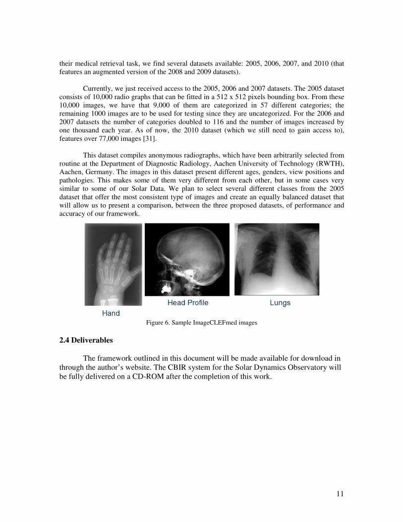
This dataset compiles anonymous radiographs, which have been arbitrarily selected from

routine at the Department of Diagnostic Radiology, Aachen University of Technology (RWTH),

Aachen, Germany. The images in this dataset present different ages, genders, view positions and

pathologies. This makes some of them very different from each other, but in some cases very

similar to some of our Solar Data. We plan to select several different classes from the 2005

dataset that offer the most consistent type of images and create an equally balanced dataset that

will allow us to present a comparison, between the three proposed datasets, of performance and

accuracy of our framework.

Figure 6. Sample ImageCLEFmed images

2.4 Deliverables

The framework outlined in this document will be made available for download in

through the author’s website. The CBIR system for the Solar Dynamics Observatory will

be fully delivered on a CD-ROM after the completion of this work.

12

3. Background Information

For this section we have separate the way we present our literature review and

background information with regards our domain-specific application and the main components

incorporated to our framework.

3.1. Activity in the solar community

In recent years, multiple attempts were made to automatically identify specific types of

phenomena from solar images. Zharkova et al. [10] using Neural Networks, Bayesian

interference, and shape correlation, have detected phenomena including sunspots, flares and,

coronal mass ejections. Zharkova and Schetinn [32] have trained a neural network to identify

filaments within solar images. Wavelet analysis was used by Delouille [33] along with the

CLARA clustering algorithm to segment mosaics of the sun. Irbah et al. [34] have also used

wavelet transforms to remove image defects (parasite spots) and noise without reducing image

resolution for feature extraction. Bojar and Nieniewski, [35] modeled the spectrum of the discrete

Fourier transform of solar images and discussed various quality measures. However, we are not

aware of any single technique reported as effective in finding a variety of phenomena and no

experiments have been performed on the size of repository even comparable to the dataset we

will have to deal with.

Automatically detecting individual phenomena in solar images has become a popular

topic in recent years. Zharkova et al. [10] discuss several methods for identifying features in solar

images including Artificial Neural Networks, Bayesian interference, and shape correlation

analyzing five different phenomena: sunspots, inference, plage, coronal mass ejections, and

flares. Automatic identification of flares, on the SDO mission, will be performed by an algorithm

created by Christe et al. [36] which works well for noisy and background-affected light curves.

This approach will allow detection of simultaneous flares in different active regions. Filament

detection for the SDO mission will be provided by the “Advanced Automated Filament Detection

and Characterization Code” [37]. The algorithm goes beyond the typical filament identification, it

determines its spine and orientation angle, finds its magnetic chirality (sense of twist), and tracks

it from image to image for as long as they are visible on the solar disk. Additionally, if a filament

is broken up into two or more pieces it can correctly identify them as a single entity. As for the

coronal jet detection and parameter determination algorithms, they will work on data cubes

covering a box enclosing the bright point and extending forward in time. SDO methods for

determining the coronal jet parameters are described in detail in [38]. Oscillations on the SDO

pipeline will be detected using algorithms presented on [39] and [40] that consist of Wavelet

transform analysis. In order to detect active regions the SDO pipeline will use the Spatial

Possibilistic Clustering Algorithm (SPoCA) that was developed by Barra et al., this algorithm

produces a segmentation of EUV solar images into classes corresponding to active region,

coronal hole and quiet sun.

As we can clearly see, the majority of currently popular approaches deal with the

recognition of individual phenomena and a few of them have demanding computational costs, not

until recently Lamb et al. [9] discussed creating an example based Image Retrieval System for the

TRACE repository. This is the only attempt, we are aware of, that involves trying to find a variety

of phenomena, with expectation of building a large-scale CBIR system for solar physicists.

13

3.2. Image descriptors/parameters

Based on our literature review, we decided that we would use some of the most popular

image parameters used in different fields such as medical images, text recognition, natural scene

images and traffic images [6, 41, 42, 43, 44, 45, 46, 47, 48, 49, 51, 52, 53], as a common

denominator the usefulness of all these image parameters have shown to be very domain

dependent.

The ten image parameters that we have included as a default in our framework are: the

Mean intensity, the Standard Deviation of the intensity, the Third Moment and Fourth Moment,

Uniformity, Entropy, and Relative Smoothness, Fractal Dimension [54], as seen in table 3, and

two Tamura texture attributes: Contrast and Directionality [55].

Table 3: Extracted Image Texture Parameters

Name Equation [11]

Mean ∑−

==

1

0

1 L

i izL

m (1)

Standard Deviation ( )∑−

=−=

1

0

21 L

i i mzL

σ (2)

Third Moment ( )∑−

=−=

1

0

3

3 )(L

i ii zpmzµ (3)

Fourth Moment ( )∑−

=−=

1

0

4

4 )(L

i ii zpmzµ (4)

Relative Smoothness (RS) )(1

11

2z

Rσ+

−= (5)

Entropy )(log)( 2

1

0 i

L

i i zpzpE ∑−

=−= (6)

Uniformity )()( 21

0 i

L

i i zpzpU ∑−

== (7)

Fractal Dimension [54]

∈

∈=

∈→ 1log

)(loglim

00

ND

(8)

Where L stands for the number of elements in the image represented as a vector and z represents a particular element in

this matrix. The Fractal Dimension is calculated based on the Box Counting dimension [54], where є is size of the

boxes.

In [55] the authors propose six texture features corresponding to human visual

perception: coarseness, contrast, directionality, line-likeness, regularity, and roughness. From

experiments used to test the significance of these features with respect to human perception, it as

concluded [6] that the first three features are very important.

The Gabor Vector was calculated by computing signatures based on Gabor texture filter.

This signature is an estimate of the amount of the texture energy passes through the Gabor filter

of a given frequency. In our experiment we used seven different frequencies

The values produced by our texture feature extraction formulas are not influenced by different

orientations of the same kinds of phenomena in different images [56]. Values for these features

can also be extracted from the images quickly [9].

3.3. Unsupervised Attribute Evaluation

Automatic methods for image parameter selection have been proposed in [57, 58].

However, these automatic methods do not directly explain why features are chosen. The method

14

proposed in [6] analyses correlations between the values of the parameters themselves, and

instead of automatically selecting a set of features, provides the user with information to help

them select an appropriate set of features.

To analyze the correlation between different image parameters, we evaluate the

correlation between the Euclidean distances d(q,X) obtained for each image parameter of each of

the images X from the our benchmark given a query image q. For each pair of query image q and

database image X we create a vector (d1(q,X), d2(q,X), . . . dm(q,X), . . . dM(q,X)) where dm(q,X) is

the distance of the query image q to the benchmark image X for the mth image parameter, and M

is the total number of image parameters. Then we calculate the correlation between the dm over all

queries q = {q1, . . . , ql, . . . qL} and all images X = {X1, . . . ,Xn, . . . ,XN}.

The M×M covariance matrix, denoted as Σij of the dm is calculated over all N database images and

all L query images as:

∑∑==

−⋅−=∑L

l

jnljinli

N

n

ij XqdXqdNL 11

)),()),((1

µµ (1)

with 1 1

1( , )

N L

i i l n

n l

d q XNL

µ= =

= ∑ ∑ (2)

Given the covariance matrix ∑ij, we calculate the correlation matrix R as Rij = ij

ii jj

∑

∑ ∑ (3)

The entries of this correlation matrix can be interpreted as similarities of different

features. A high value Rij means a high similarity between features i and j. This similarity matrix

can then be analyzed to find out which of our parameters have highly correlated values and which

do not.

3.4. Supervised Attribute Evaluation

Chi Squared: This method evaluates the worth of an attribute by computing the value of the chi-

squared distribution with respect to the class [59].

Gain Ratio: This method valuates the worth of an attribute by measuring the gain ratio with

respect to the class [60]. This method biases the decision tree against considering attributes with a

large number of distinct values. Solving the weakness presented by the information gain method

that when applied to attributes that can take on a large number of distinct values might memorize

training set too well.

Info Gain: This method evaluates the worth of an attribute by measuring the information gain

with respect to the class [59]. Like previously mentioned a notable problem occurs when

information gain is applied to attributes that can take on a large number of distinct values.

3.5. Dissimilarity Measures

We selected twelve dissimilarity measures to use for comparison purposes. Based on our

literature review, we believe that the measures selected are widely used in image analysis and

produce good results when applied to images in other domains [61, 62, 63]. Since we work on

very similar image data we decided to investigate different measures in order to verify how well

15

they differentiate our images between our solar phenomena classes and mark similarities within

the classes themselves. We will address this later in our experiment section, where we present

plots of dissimilarity matrices.

For the first eight measures given an m-by-n data matrix X (in our case it contains

m=1600 histograms and n=64 bins), which is treated as m (1-by-n) row vectors x1, x2, ..., xm, the

various distances between the vector xs and xt are defined as follows:

Euclidean distance [12]: Defined as the distance between two points give by the Pythagorean

Theorem. Special case of the Minkowski metric where p=2.

)')(( tstsst xxxxD −−= (4)

Standardized Euclidean distance [12]: Defined as the Euclidean distance calculated on

standardized data, in this case standardized by the standard deviations.

)'()( 1

tstsst xxVxxD −−= − (5)

Where V is the n-by-n diagonal matrix whose jth diagonal element is S(j)

2, where S is the vector of

standard deviations.

Mahalanobis distance [12]: Defined as the Euclidean distance normalized based on a covariance

matrix to make the distance metric scale-invariant.

)'()( 1

tstsst xxCxxD −−= − (6)

Where C is the covariance matrix

City block distance [12]: Also known as Manhattan distance, it represents distance between

points in a grid by examining the absolute differences between coordinates of a pair of objects.

Special case of the Minkowski metric where p=1.

∑=

−=n

j

tjsjst xxD1

(7)

Chebychev distance [12]: Measures distance assuming only the most significant dimension is

relevant. Special case of the Minkowski metric where p = ∞.

{ }tjsjjst xxD −= max (8)

Cosine distance [64]: Measures the dissimilarity between two vectors by finding the cosine of the

angle between them.

)')('(

'1

ttss

tsst

xxxx

xxD −= (9)

Correlation distance [64]: Measures the dissimilarity of the sample correlation between points as

sequences of values.

16

)')(()')((

)')((1

ttttssss

ttssst

xxxxxxxx

xxxxD

−−−−

−−−= (10)

Where ∑=

=n

j

sjs xn

x1

1 and ∑

=

=n

j

tjt xn

x1

1

Spearman distance [65]: Measures the dissimilarity of the sample’s Spearman rank [25]

correlation between observations as sequences of values.

)')(()')((

)')((1

ttttssss

ttssst

rrrrrrrr

rrrrD

−−−−

−−−= (11)

Where rsj is the rank of xsj taken over x1j, x2j, ...xmj, rs and rt are the coordinate-wise rank vectors of

xs and xt, i.e., rs = (rs1, rs2, ... rsn) and ∑∑==

+==

+==

n

j

tjt

n

j

sjs

nr

nr

nr

nr

11 2

)1(1,

2

)1(1

Since our focus is on comparing image histograms, we present the next for measures in

terms of histograms.

Hausdorff Distance [15]: Intuitively defined as the maximum distance of a histogram to the

nearest point in the other histogram.

)},(infsup),,(infsupmax{)',(''

yxdyxdHHDHHxHyHyHx ∈∈∈∈

= (12)

Where sup represents the supremum, inf the infimum, and d(x,y) represents any distance measure

between two points, in our case we used Euclidean distance.

Jensen–Shannon divergence (JSD) [13]: Also known as total divergence to the average, Jensen–

Shannon divergence is a symmetrized and smoothed version of the Kullback–Leibler divergence.

(13)

2χ distance [92]: Measures the likeliness of one histogram being drawn from another one.

∑= +

−=

n

m mm

mm

HH

HHHH

1

2

'

')',(χ (14)

Kullback–Leibler divergence (KLD) [14]: Measures the difference between two histograms H

and H’. Often intuited as a distance metric, the KL divergence is not a true metric since the KL

divergence from H to H’ is not necessarily the same as the KL divergence from H’ to H.

(15)

∑

=

=n

m m

mm

H

HHHHKL

1

log)',(

∑= +

++

=n

m mm

mm

mm

mm

HH

HH

HH

HHHHJD

1 '

'2log'

'

2log)',(

17

Since this is the only non-symmetric measure we used for this work. We treated it as a

directed measure and considered H-H’ and H’-H as two different distances.

3.6. Dimensionality reduction

Some comparisons between dimensionality reduction methods for image retrieval have

been performed in the past [66, 67, 68, 69, 70], but none of them report results on solar image

data. However, these works constantly encounter the fact that results are very domain-specific

and that performance of the non-linear versus linear dimensionality reduction methods has been

shown to be dependent of the nature of the dataset (natural vs. artificial) [71]. Most of these

works also determine that PCA is in general one of the best performing dimensionality reductions

methods when compared to non-linear dimensionality reduction methods.

Based on our literature review, we decided to utilize four different linear and four non-linear dimensionality reduction methods. Based on previous works [67, 70, 71] linear dimensionality reduction methods have been proved to perform better than non-linear methods in most artificial datasets and some natural datasets, however all these results have been domain dependent. Classical methods like PCA and SVD are widely used as benchmarks to provide a comparison versus the newer non-linear methods. We selected our eight different methods based on their popularity in the literature, the availability of a mapping function or method to map new unseen data points into the new dimensional space, computational expense, and the particular properties of some methods such as the preservation of local properties between the data and the type of distances between the data points (Euclidean versus geodesic). 3.6.1. Linear dimensionality reduction methods

Principal Component Analysis (PCA) [16]

PCA is defined as an orthogonal linear transformation that transforms data into an

artificial space such that the greatest variance by any projection of the data comes to lie on the first principal component, and so on.

For a data matrix, M

T, where each row represents a different observation on the dataset,

and each column contains the variables, the PCA transformation is given by:

TTTVUMY ∑== (16)

Where the matrix Σ is an m-by-n diagonal matrix with nonnegative real numbers on the diagonal and UΣ V

T is the singular value decomposition of M.

Singular Value Decomposition (SVD) [72]

Defined for a m-by-n matrix M as the factorization of the form:

TVUM ∑= (17)

Where U is an m-by-m unitary matrix, the matrix Σ is m-by-n diagonal matrix with nonnegative real numbers on the diagonal, and V

T denotes the conjugate transpose of V, an n-by-n

unitary matrix.

18

Normally, the diagonal entries ∑i,i are ordered in a descending way. This diagonal matrix ∑ is uniquely determined by M and the diagonal entries are the singular values of M. The columns of V form a set of orthonormal input basis vector directions for M. (The eigenvectors of M

TM.) The

columns of U form a set of orthonormal output basis vector directions for M. (The eigenvectors of MM

T )

NOTE: The main difference from a practical point of view, between PCA and SVD is that SVD is directly applied to an m-by-n matrix (i.e. m-by-n long feature vectors), while in PCA, SVD is applied to a covariance matrix (n-by-n). This results with the starting matrix being different in each case.

Locality Preserving Projections (LPP) [73]

LPP generates linear projective maps by solving a variational problem that optimally

preserves the neighborhood structure of a dataset. These projections are obtained by embedding the optimal linear approximations to the eigenfunctions of the Laplace Beltrami operator on the manifold. The resulting mapping corresponds to the following eigenvalue problem:

wMDXwMLMTT λ= (18)

Where L is the Laplacian matrix, (i.e. D – S, where S corresponds to the similarity values defined, and D is a column matrix which reflects how important certain projections are). The more data points that surround a given point, the more importance they have, preserving locality. LPP is defined everywhere in the ambient space, not only on the training data points like Isomaps, LLE, and Laplacian Eigenmaps. LPP is also capable of discovering a nonlinear structure of the data manifold; therefore it can approximate non-linear methods in a faster and more practical way to compute.

Factor Analysis (FA) [74]

FA is a statistical method used to describe variability among observed variables in terms

of a potentially lower number of unobserved variables called factors. The observed variables are modeled as linear combinations of the potential factors, plus error terms. The information gained about the interdependencies between observed variables is used later to reduce the set of variables in a dataset, achieving dimensionality reduction.

To perform FA we compute the maximum likelihood estimate of the factor loadings matrix Λ in the factor analysis model

efM +Λ+= µ (19)

Where M is the m-by-n data matrix, µ is a constant vector of means, Λ is a constant m-by-n matrix of factor loadings, f is a vector of independent and standardized common factors, and e is a vector of independent specific factors. M, µ, and e are of length m. f is of length n.

FA is related to PCA since PCA performs a variance-maximizing rotation of the variable space, taking into account all variability in the variables. On the other hand, factor analysis estimates how much of the variability is due to common factors.

3.6.2. Non-linear dimensionality reduction methods Kernel PCA [75]

Kernel PCA computes the principal eigenvectors of the kernel matrix, rather than those of

the covariance matrix. The reformulation of PCA in kernel space is straightforward, since a kernel

19

matrix is similar to the inner-product of the data points in the high dimensional space that is constructed using the kernel function. The application of PCA in the kernel space provides Kernel PCA the property of constructing nonlinear mappings.

Kernel PCA computes the kernel matrix K of the data-points xi. The entries in the kernel

matrix are defined by

),(, jiji xxk = (20)

Where kj,i is a kernel function. Then the kernel matrix K is centered by subtracting the

mean of the features in traditional PCA. Then the principal d eigenvectors vi of the centered kernel matrix are computed. Finally, the eigenvectors of the covariance matrix αi in the high-dimensional space constructed by k can now be computed by (6), since they are related to the eigenvectors vi of the matrix K.

i

i

i Mvλ

α1

= (21)

To obtain the low-dimensional data representation, the data is projected onto the

eigenvectors of the covariance matrix αi. The entries of Y, the low dimensional representation are given by:

= ∑ ∑= =

n

j

n

j

ij

j

dij

j

i xxkxxky1 1

1 ),(),....,,( αα (22)

Where α1

j indicates the jth value in the vector α1 and k is the kernel function used in the

computation of the kernel matrix.

Since Kernel PCA is a kernel-based method, the mapping performed by Kernel PCA relies on the choice of the kernel function k. For this work we utilized a Gaussian kernel. Isomap [76]

Isomap preserves pair-wise geodesic distances between data points. The geodesic

distances between the data points xi of M are calculated by constructing a neighborhood graph G, in which every data point xi is connected with its k nearest neighbor’s xij in the dataset M. The shortest path between two points in the graph forms a good estimate of the geodesic distance between these two points, and can easily be calculated forming a pair-wise m-by-m geodesic adjacency matrix. The low-dimensional representations yi of the data point’s xi in the low-dimensional space Y are computed by applying multidimensional scaling (MDS) [29] on the resulting m-by-m geodesic adjacency matrix.

Locally-Linear Embedding (LLE) [18]

Similarly to Isomap, LLE constructs a graph representation of the data points and attempts to preserve the local properties of the data allowing for successful embedding of non-convex manifolds. In LLE, the local properties of the data are constructed by writing linear combinations of the nearest neighbors of the data points. In the low-dimensional representation of the data, this

20

method retains the reconstruction weights in the linear combinations. The method writes the local properties of the manifold around a data point xi by writing the data point as a linear combination Wi of its k nearest neighbors xij, by fitting an hyperplane through the data point xi and its nearest neighbors assuming that the manifold is locally linear. This local linearity assumption implies that the reconstruction weights Wi of the data points xi are invariant to translation, rotation, and rescaling. If the low-dimensional data representation preserves the local geometry of the manifold, the reconstruction weights Wi that reconstruct data point xi from its neighbors in the high-dimensional representation also reconstruct data point yi from its neighbors in the low-dimensional representation. Therefore finding the d dimensional data representation Y depends on minimizing the cost function

∑ ∑=

−=i

k

j

ijiji ywyY1

2)()(φ (23)

Where yi is a data point in the low dimensional representation and wij is a reconstruction weight.

Laplacian Eigenmaps (LE) [17]

LE is another method that preserves the local properties of the manifold to produce a low-

dimensional data representation. These local properties are based on the pair-wise distances between k nearest neighbors. LE computes a low-dimensional representation of the data minimizing the distances between a data point and its k nearest neighbors. The contribution of each distance depends on the proximity of the particular nearest neighbor to the data point.

The LE algorithm first constructs a neighborhood graph G in which every data point xi is

connected to its k nearest neighbors. The weights of the edges on the connected data points of G are computed using the Gaussian kernel function, resulting in an adjacency matrix W. The computation of the degree matrix M and the graph Laplacian L of the graph W allows for the formulation of the minimization problem (needed to compute the low-dimensional representations) as an eigenproblem. The degree matrix M is a diagonal matrix, of which the entries consist of the row sums of W. The Laplacian L of the graph is computed by L = M − W. The low-dimensional representation Y can be found by solving the generalized eigenvalue problem:

MvLv λ= (24)

For the d smallest nonzero eigenvalues, where d is the number of desired dimensions for Y. The d eigenvectors vi corresponding to the smallest nonzero eigenvalues form the low-dimensional representation Y.

3.7. Indexing techniques

3.7.1. Single-Dimensional Indexing for Multi-Dimensional Data

B+ Trees

B+ Trees are indexing structures that represent sorted data allowing for efficient

insertion, retrieval and deletion of records, each identified by a key. The B+ Tree is dynamic and

multilevel, having maximum and minimum bounds on the number of keys in each index segment.

In contrast to a B-tree, all records are stored at the leaf level of the tree; only keys are stored in

21

interior nodes. The notion of the B+ Trees was first brought up by Corner [77], as an interesting

alternative for B Trees, but it was never introduced as a formal concept.

Due to the popularity and efficiency of B+ Trees, they have been implemented in many

relational database management systems for table indices, such as: IBM DB2, Informix,

Microsoft SQL Server, Oracle 8, PostgreSQL, MySQL and SQLite.

B+ Trees have been mainly utilized to index one-dimensional data; however, many of the

high-dimensional indexing techniques employ B+ Trees after they have broken down the

dimensionality of the dataset into segments that can be indexed by a B+ Tree [78, 80, 81, 82, 83].

iDistance [78, 79]

iDistance is an indexing and query processing technique for k-nearest neighbor queries

on point data in multi-dimensional metric spaces. The algorithm is designed to process kNN

queries in high-dimensional spaces efficiently and it is especially good for skewed data

distributions, which usually occur in real-life data sets.

In order to build the iDistance index, there are two steps involved:

1) A certain number of reference points in the original data space are chosen by using

cluster centers as reference points, since according to the author’s research [78, 79] this is

the most efficient way of doing so.

2) The distance between a data point and its closest reference point is calculated (using

the Euclidean distance), this distance plus a scaling value is then called the iDistance.

In this way, we observe that points in a multi-dimensional space are mapped to one-

dimensional values allowing us to use a B+-tree can to index these points using the iDistance as

the key.

To process a kNN query, the query is mapped to several one-dimensional range queries

that can be processed efficiently on a B+-tree. A query Q is mapped to a value in the B+-tree

while the kNN search sphere is mapped to a range in the B+-tree. The search sphere expands

gradually until the kNN’s are found corresponding to gradually expanding range searches in the

B+-tree. This iDistance technique can be viewed as a way of accelerating the sequential scan

since instead of scanning records from the beginning to the end of the data file, iDistance starts

the scan from places where the nearest neighbors can be obtained early with a very high

probability.

iMinMax [80]

iMinMax is an indexing and query processing technique that focuses on “indexing on the

edge”. The edge refers to the maximum or minimum values among all the dimensions of said

data point. iMinMax(θ) uses either the values of the Max edge (the dimension with the maximum

value) or the values of the Min edge (the dimension with the minimum value) as the

representative index keys for the points. Because the transformed values can be ordered and range

22

queries can be performed on the transformed (single dimensional) space, we can employ single

dimensional indexes to index the transformed values.

iMinMax(θ) uses a very simple mapping function that is computationally inexpensive.

The data point x is mapped to a point y over a single dimensional space in the following manner:

+

−<++=

otherwisexd

xxifxdy

maxmax

maxminminmin 1θ (25)

Where θ is a real number playing an important role in influencing the number of points

falling on each index hyper plane.

This transformation actually splits the (single dimensional) data space into different

partitions based on the dimension which has the largest value or smallest value, and provides an

ordering within each partition. The configurable feature (the θ) of iMinMax facilitates the

adaptation of data sets featuring different types of distributions (uniform or skewed). In cases

where data points are skewed toward certain edges, we may “scatter" these points to other edges

to evenly distribute them by making a choice between dmin and dmax.

As for querying, the queries on the original space need to be transformed. For a given

range query, the range of each dimension is used to generate a particular range sub-queries on

that dimension. The union of the answers from all sub-queries provides a candidate answer set

from which the query answers can be obtained. iMinMax's query mapping function facilitates

effective range query processing because the search space on the transformed space contains all

answers from the original query. The number of points within a search space is reduced allowing

some of the sub-queries to be pruned away without being evaluated.

UB-Trees [81]

First introduced by Rudolf Bayer and Volker Markl [81], the UB-Tree is a balanced tree

for storing and efficiently retrieving multidimensional data. With its foundation on B+ trees, since

the information is only stored in the leaves, the records are stored using a Z-order, also called

Morton order. This Z-order is calculated by bitwise interlacing of the keys. Insertion, deletion,

and point queries are performed in the same ways as B+ trees. To perform range searches in

multidimensional point data, there is an algorithm that calculates based on a point encountered in

the database, the next Z-value which is in the multidimensional search range.

Originally to solve this key problem the computational time was exponential with respect

to the dimensionality hence very computationally expensive [81]. A proposed solution to the

problem that is linear with the z-address bit length was described in [84].

Pyramid-trees [83]

Pyramid-trees map a d-dimensional point into a 1-dimensional space and use a B+-tree to

index the 1-dimensional space. In Pyramid trees, queries have to be translated in a similar

fashion, in the data pages of the B+-tree, Pyramid-trees stores both the d-dimensional points and

the 1-dimensional key. This allows Pyramid Trees to not require inverse transformation and the

23

refinement step can be performed without look-ups to another file or structure. This mapping is

called Pyramid-mapping and it’s based on a partitioning strategy that is optimized for range

queries on high-dimensional data. The basic idea of this Pyramid-mapping is to divide the data

space in a way that the resulting partitions are shaped like peels of an onion, allowing them to be

indexed by B+-trees in a very efficient manner.

Pyramid-trees are one of the only indexing structures known that are not affected by the

“curse of dimensionality”, meaning that for uniform data and range queries, the performance of

Pyramid-trees gets even better if one increases the dimensionality, in [85] there is an analytical

explanation of this occurrence.

3.7.2. Multi-Dimensional Indexing

R-trees [86]

R-trees are indexing data structures that are similar to B-trees, but are used for indexing

multi-dimensional information. R-trees split space with hierarchically nested, Minimum

Bounding Rectangles (MBRs). Overlapping between regions in different branches is allowed, but

they deteriorate the search performance. This is a problem that becomes more evident as the

number of dimension increases [87]. The region description of an MBR comprises for each

dimension a lower and an upper bound. Thus, 2-d floating point values are required.

Due to this overlapping problem, several improvements over the original R-tree

algorithm have been proposed in order to address these performance issues. We will discuss two

of these improvements (R+-trees and R*-trees) and their advantages in the next few paragraphs.

The R+-tree [88] is an overlap-free variant of the R-tree. In order to guarantee no overlap,

the splitting algorithm is modified by a forced-split strategy. In this strategy, the child pages

which are an obstacle in overlap-free splitting of some pages are simply cut into two pieces at a

particular position. This might require that these forced splits must be propagated down until the

data page level is reached, allowing the number of pages to exponentially increase from level to

level. This extension of the child pages is not much smaller than the extension of the parent page

if the dimensions in the data are sufficiently high.

Allowing many forced split operations, the pages which are subject to a forced split, are

split, although no overflow has occurred, this results in the pages being utilized by less than 50%.

The more forced splits that are required, the more the storage utilization of the complete index

will deteriorate.

The R*-tree [89] attempts to reduce both coverage and overlap problems by using a

combination of a revised node split algorithm and the concept of forced re-insertion at node

overflow. Based on the observation that R-tree structures are highly susceptible to the order in

which their entries are inserted, an insertion-built structure is not likely to be optimal. The

deletion and re-insertion of entries allows them to locate a position in the tree that may be more

optimal than their original location.

When a node overflows, a portion of its entries are removed from the node and re-

inserted into the tree, to avoid an indefinite cascade of reinsertions caused by subsequent node

24

overflow, the reinsertion routine may be called only once in each level of the tree when inserting

any new entry. This produces more well-clustered groups of entries in nodes and reduces the node

coverage. Actual node splits are often postponed, causing the average node occupancy to rise. Re-

insertion can be seen as a method of incremental tree optimization triggered on node overflow.

This provides a significant improvement over previous R-tree variants, but the overhead comes

because of the reinsertion method.

Empirical analyses [87, 90] show that R-trees, R+-trees, and R*-trees do not perform well

when indexing high-dimensional data sets (i.e. more than four dimensions). The main problem

with R-tree-based indexes is that the overlap of the bounding boxes in the directory increases

with growing dimension, quickly creating problems when querying in these overlapping

bounding boxes.

TV-trees [91]

TV-Trees are designed particularly for real data sets subject to the Karhunen-Loeve

Transform, which is a dimensionality reduction technique that preserves distances and eliminates

linear correlations. Such data sets yield high variance allowing for a good selectivity in the first

few dimensions (principal components) while the last few dimensions are of minor importance

since very little of the variance is left in them.

Regions of the TV-tree are described using vectors that might be dynamically shortened

called Telescope Vectors (TV). A region has k inactive dimensions and α active dimensions. The

inactive dimensions form the greatest common prefix of the vectors stored in the subtree. The

extension of the region is zero in inactive dimensions, in the α active dimensions, the region has

the form of an Lp-sphere, where p may be 1, 2 or ∞. Allowing the region to have an infinite

extension in the remaining dimensions, which might be active in the lower levels of the index, or

have minor importance for query processing.

The region descriptor has α floating point values for the coordinates of the center point in

the active dimensions and one floating point value for the radius. The coordinates of the inactive

dimensions are stored in higher levels of the index (exactly in the level where a dimension

changes from active into inactive). The concept of telescope vectors increases the capacity of the

directory pages.

X-trees [87]

X-trees are based on the R-trees family, but they differ in that the X-tree emphasizes

prevention of overlap in the bounding boxes, a problem that increases in high dimensions. In the

cases where the nodes cannot be split without preventing overlap, the node split will be delayed,

this results in super-nodes. In a worst-case scenario, the tree will linearize, allowing it to perform

better than other worst-case scenarios observed in some other data structures.

The primary modification to R*-trees, the splitting algorithm, works as follows: In case

of a data page split, the X-trees use the R*-tree split algorithm or any other topological split

algorithm. In case of directory nodes, the X-trees try to split the node using a topological split

algorithm, if this split results in highly overlapping Minimum Bound Rectangles (MBR), the X-

25

trees apply the overlap-free split algorithm based on the split history. If this leads to an

unbalanced directory then the X-tree creates a super-node.

X-trees show a high performance gain compared to R*-trees for all query types in

medium dimensional spaces [87]. For a small number of dimensions, X-Trees show a behavior

nearly identical to R-trees. For higher dimensions, X-trees have to visit so large a number of

nodes that a linear scan is considered less expensive.

26

References

[1] R. Datta, D. Joshi, J. Li and J. Wang, “Image Retrieval: Ideas, Influences, and Trends of the

New Age”, ACM Computing Surveys, vol. 40, no. 2, article 5, pp. 1-60, 2008.

[2] Y. Rui, T.S. Huang, S. Chang, “Image Retrieval: Current Techniques, Promising Directions,

and Open Issues”. Journal of Visual Communication and Image Representation 10, pp. 39–62,

1999.

[3] H. Müller, N. Michoux, D. Bandon, A. Geissbuhler, “A review of content-based image

retrieval systems in medical applications: clinical benefits and future directions”. International

journal of medical informatics, Volume 73, pp. 1-23, 2004

[4] Y.A Aslandogan, C.T Yu, “Techniques and systems for image and video retrieval” IEEE

Transactions on Knowledge and Data Engineering, Vol: 11 1 , Jan.-Feb. 1999.

[5] A. Yoshitaka, T. Ichikawa “A survey on content-based retrieval for multimedia databases”

IEEE Transactions on Knowledge and Data Engineering, Vol: 11 1 , Jan.-Feb. 1999.

[6] T. Deselaers, D. Keysers, and H. Ney, "Features for Image Retrieval: An Experimental

Comparison", Information Retrieval, Vol. 11, issue 2, The Netherlands, Springer, pp. 77-107,

2008.

[7] H. Müller, A. Rosset, J-P. Vallée, A. Geissbuhler, Comparing feature sets for content-based

medical information retrieval. SPIE Medical Imaging, San Diego, CA, USA, February 2004.

[8] S. Antani, L.R. Long, G. Thomas. "Content-Based Image Retrieval for Large Biomedical

Image Archives" Proceedings of 11th World Congress on Medical Informatics (MEDINFO) 2004

Imaging Informatics. September 7-11 2004; San Francisco, CA, USA. 829-33. 2004.

[9] R. Lamb, “An Information Retrieval System For Images From The Trace Satellite,” M.S.

thesis, Dept. Comp. Sci., Montana State Univ., Bozeman, MT, 2008.

[10] V. Zharkova, S. Ipson, A. Benkhalil and S. Zharkov, “Feature recognition in solar images,"

Artif. Intell. Rev., vol. 23, no. 3, pp. 209-266. 2005.

[11] M. Hall, E. Frank, G. Holmes, B. Pfahringer, P. Reutemann, I. H. Witten. “The WEKA Data

Mining Software: An Update” SIGKDD Explorations, Volume 11, Issue 1, 2009

[12] K. Yang, J. Trewn. Multivariate Statistical Methods in Quality Management. McGraw-Hill

Professional; pp. 183-185. 2004.

[13] J. Lin. "Divergence measures based on the shannon entropy". IEEE Transactions on

Information Theory 37 (1): pp. 145–151. 2001.

[14] S. Kullback, R.A. Leibler "On Information and Sufficiency". Annals of Mathematical

Statistics 22 (1): pp. 79–86. 1951.

27

[15] J. Munkres. Topology (2nd edition). Prentice Hall, pp 280-281. 1999.

[16] K. Pearson, "On lines and planes of closest fit to systems of points in space" . Philosophical

Magazine 2 (6) 1901, pp 559–572.

[17] M. Belkin and P. Niyogi. Laplacian Eigenmaps and spectral techniques for embedding and

clustering. In Advances in Neural Information Processing Systems, volume 14, pp. 585–591,

Cambridge, MA, USA. The MIT Press. 2002.

[18] L.K. Saul, K.Q. Weinberger, J.H. Ham, F. Sha, and D.D. Lee. Spectral methods for

dimensionality reduction. In Semisupervised Learning, Cambridge, MA, USA, The MIT Press.

2006.

[19] T. Etzold, A. Ulyanov, P. Argos. "SRS: information retrieval system for molecular biology

data banks". Methods Enzymol. pp. 114–128. 1999

[20] D. S. Raicu, J. D. Furst, D. Channin, D. H. Xu, & A. Kurani, "A Texture Dictionary for

Human Organs Tissues' Classification", Proceedings of the 8th World Multiconference on

Systemics, Cybernetics and Informatics (SCI 2004), Orlando, USA, in July 18-21, 2004.

[21] P. Korn, N. Sidiropoulos, C. Faloutsos, E. Siegel, and Z. Protopapas,"Fast and effective

retrieval of medical tumor shapes," IEEE Transactions on Knowledge and Data Engineering, vol.

10, no. 6, pp.889-904. 1998.

[22] J. M. Banda and R. Anrgyk “An Experimental Evaluation of Popular Image Parameters for

Monochromatic Solar Image Categorization”. FLAIRS-23: Proceedings of the twenty-third

international Florida Artificial Intelligence Research Society conference, Daytona Beach, Florida,

USA, May 19–21 2010. 2010.

[23] Heliophysics Event Registry [Online] Available:

http://www.lmsal.com/~cheung/hpkb/index.html [Accessed: Sep 24, 2010]

[24] TRACE On-line (TRACE) [Online], Available: http://trace.lmsal.com/. [Accessed: Sep 29,

2010]

[25] TRACE Data set (MSU) [Online], Available:

http://www.cs.montana.edu/angryk/SDO/data/TRACEbenchmark/ [Accessed: Sep 29, 2010]

[26] J.M Banda and R. Angryk “On the effectiveness of fuzzy clustering as a data discretization

technique for large-scale classification of solar images” Proceedings of the 18th IEEE

International Conference on Fuzzy Systems (FUZZ-IEEE ’09), Jeju Island, Korea, August 2009,

pp. 2019-2024. 2009.

[27] A. Pronobis, B. Caputo, P. Jensfelt, and H. I. Christensen. “A discriminative approach to

robust visual place recognition”. In Proceedings of the IEEE/RSJ International Conference on

Intelligent Robots and Systems (IROS06), Beijing, China, 2006.

[28] The INDECS Database [Online], Available:

http://cogvis.nada.kth.se/INDECS/ [Accessed: Sep 29, 2010]

28

[29] W. Hersh, H. Müller, J. Kalpathy-Cramer, E. Kim, X. Zhou, “The consolidated

ImageCLEFmed Medical Image Retrieval Task Test Collection”, Journal of Digital Imaging,

volume 22(6), 2009, pp 648-655.

[30] Cross Language Evaluation Forum [Online], Available:

http://www.clef-campaign.org/ [Accessed: Sep 29, 2010]

[31] Image CLEF – Image Retrieval in CLEF, Available:

http://www.imageclef.org/2010/medical [Accessed: Sep 29, 2010]

[32] V. Zharkova and V. Schetinin, “Filament recognition in solar images with the neural

network technique," Solar Physics, vol. V228, no. 1, 2005, pp. 137-148. 2005.

[33] V. Delouille, J. Patoul, J. Hochedez, L. Jacques and J.P. Antoine ,“Wavelet spectrum

analysis of eit/soho images," Solar Physics, vol. V228, no. 1, 2005, pp. 301-321. 2005.

[34] A. Irbah, M. Bouzaria, L. Lakhal, R. Moussaoui, J. Borgnino, F. Laclare and C. Delmas,

“Feature extraction from solar images using wavelet transform: image cleaning for applications to

solar astrolabe experiment.” Solar Physics, Volume 185, Number 2, April 1999 , pp. 255-273(19).

1999.

[35] K. Bojar and M. Nieniewski. “Modelling the spectrum of the fourier transform of the texture

in the solar EIT images”. MG&V 15, 3, pp. 285-295. 2006.

[36] S. Christe, I. G. Hannah, S. Krucker, J. McTiernan, and R. P. Lin. “RHESSI Microflare

Statistics. I. Flare-Finding and Frequency Distributions”. ApJ, 677 pp. 1385–1394. 2008.

[37] P. N. Bernasconi, D. M. Rust, and D. Hakim. “Advanced Automated Solar Filament

Detection And Characterization Code: Description, Performance, And Results”. Sol. Phys., 228.

pp. 97–117, 2005.

[38] A. Savcheva, J. Cirtain, E. E. Deluca, L. L. Lundquist, L. Golub, M. Weber, M. Shimojo, K.

Shibasaki, T. Sakao, N. Narukage, S. Tsuneta, and R. Kano. “A Study of Polar Jet Parameters

Based on Hinode XRT Observations”. Publ. Astron. Soc. Japan, 59:771–+. 2007.

[39] I. De Moortel and R. T. J. McAteer. “Waves and wavelets: An automated detection

technique for solar oscillations”. Sol. Phys., 223. pp. 1–2. 2004.

[40] R. T. J. McAteer, P. T. Gallagher, D. S. Bloomfield, D. R. Williams, M. Mathioudakis, and

F. P. Keenan. “Ultraviolet Oscillations in the Chromosphere of the Quiet Sun”. ApJ, 602, pp.

436–445. 2004.

[41] S. Kulkarni, B. Verma, "Fuzzy Logic Based Texture Queries for CBIR," Fifth International

Conference on Computational Intelligence and Multimedia Applications (ICCIMA'03), pp.223,

2003

29

[42] H Lin, C Chiu, and S. Yang, “LinStar texture: a fuzzy logic CBIR system for textures”, In

Proceedings of the Ninth ACM international Conference on Multimedia (Ottawa, Canada).

MULTIMEDIA '01, vol. 9. ACM, New York, NY, pp 499-501. 2001.

[43] S. Thumfart, W. Heidl, J. Scharinger, and C. Eitzinger. “A Quantitative Evaluation of

Texture Feature Robustness and Interpolation Behaviour”. In Proceedings of the 13th

international Conference on Computer Analysis of Images and Patterns. 2009.

[44] J. Muwei, L. Lei, G. Feng, "Texture Image Classification Using Perceptual Texture Features

and Gabor Wavelet Features," Asia-Pacific Conference on Information Processing vol. 2, pp.55-

58, 2009.

[45] E. Cernadas, P. Carriön, P. Rodriguez, E. Muriel, and T. Antequera. “Analyzing magnetic

resonance images of Iberian pork loin to predict its sensorial characteristics” Comput. Vis. Image

Underst. 98, 2 pp. 345-361. 2005.

[46] S.S. Holalu and K. Arumugam “Breast Tissue Classification Using Statistical Feature

Extraction Of Mammograms”, Medical Imaging and Information Sciences, Vol. 23 No. 3, pp.

105-107. 2006

[47] S. T. Wong, H. Leung, and H. H. Ip, “Model-based analysis of Chinese calligraphy images”

Comput. Vis. Image Underst. 109, 1 (Jan. 2008), pp. 69-85. 2008.

[48] V. Devendran, T. Hemalatha, W. Amitabh "SVM Based Hybrid Moment Features for

Natural Scene Categorization," International Conference on Computational Science and

Engineering vol. 1, pp.356-361, 2009.

[49] B. B. Chaudhuri, Nirupam Sarkar, "Texture Segmentation Using Fractal Dimension," IEEE

Transactions on Pattern Analysis and Machine Intelligence, vol. 17, no. 1, pp. 72-77, Jan. 1995

[51] C. Wen-lun, S. Zhong-ke, F. Jian, "Traffic Image Classification Method Based on Fractal

Dimension," IEEE International Conference on Cognitive Informatics Vol. 2, pp.903-907, 2006.

[52] A.P Pentland, “Fractal-based description of natural scenes’, IEEE Trans. on Pattern Analysis

and Machine Intelligence, 6 pp. 661-674, 1984.

[53] H.F. Jelinek, D.J. Cornforth, A.J. Roberts, G. Landini, P. Bourke, and A. Iorio, “Image

processing of finite size rat retinal ganglion cells using multifractal and local connected fractal

analysis”, In 17th Australian Joint Conference on Artificial Intelligence, volume 3339 of Lecture

Notes in Computer Science, pages 961--966. Springer--Verlag Heidelberg, 2004

[54] M. Schroeder. Fractals, Chaos, Power Laws: Minutes from an Infinite Paradise. New York:

W. H. Freeman, pp. 41-45, 1991.

[55] H. Tamura, S. Mori, T. Yamawaki. “Textural Features Corresponding to Visual Perception”.

IEEE Transaction on Systems, Man, and Cybernetics 8(6): pp. 460–472. 1978.

30

[56] R.M Haralick, K. Shanmugam and I. Dinstein, “Textural Features For Image Classification,”

IEEE Transactions on Systems, Man, and Cybernetics, Volume: SMC-3, No. 6, pp 610- 621.

1978.

[57] N. Vasconcelos, M. Vasconcelos. “Scalable Discriminant Feature Selection for Image

Retrieval and Recognition”. In CVPR 2004. (Washington, DC 2004), pp. 770–775. 2004.

[58] M. Schroeder. “Fractals, Chaos, Power Laws: Minutes from an Infinite Paradise”. (W. H.

Freeman, New York 1991), pp. 41-45. 1991.

[59] S. Kullback, and R.A. Leibler. “On Information and Sufficiency”. Annals of Mathematical

Statistics 22, pp. 79–86. 1951.

[60] J.R. Quinlan. “Induction of decision trees”. Machine Learning, pp. 81-106, 1986.

[61] G. D Guo, A.K. Jain, W.Y Ma, H.J Zhang,et. al, "Learning similarity measure for natural

image retrieval with relevance feedback". IEEE Transactions on Neural Networks. Volume 13

(4). pp. 811-820, 2002.

[62] R. Lam, H. Ip, K. Cheung, L. Tang, R. Hanka, "Similarity Measures for Histological Image

Retrieval," 15th International Conference on Pattern Recognition (ICPR'00) - Volume 2. pp.

2295. 2000.

[63] T. Ojala, M. Pietikainen, and D. Harwood. A comparative study of texture measures with

classification based feature distributions. Pattern Recognition, 29(1). pp. 51–59. 1996.

[64] P.-N. Tan, M. Steinbach & V. Kumar, "Introduction to Data Mining", Addison-Wesley pp.

500, 2005.

[65] C. Spearman, "The proof and measurement of association between two things" Amer. J.

Psychol. ,V 15. pp. 72–101. 1904

[66] P. Moravec, and V. Snasel, “Dimension reduction methods for image retrieval”. In

Proceedings of the Sixth international Conference on intelligent Systems Design and Applications

- Volume 02 (October 16 - 18, 2006). ISDA. IEEE Computer Society, Washington, DC, pp.

1055-1060. 2006.

[67] J. Ye, R. Janardan, and Q. Li, “GPCA: an efficient dimension reduction scheme for image

compression and retrieval”. In Proceedings of the Tenth ACM SIGKDD international Conference

on Knowledge Discovery and Data Mining (Seattle, WA, USA, August 22 - 25, 2004). KDD '04.

ACM, New York, NY, pp. 354-363. 2004.

[68] E. Bingham, and H. Mannila, “Random projection in dimensionality reduction: applications

to image and text data”. In Proceedings of the Seventh ACM SIGKDD international Conference

on Knowledge Discovery and Data Mining (San Francisco, California, August 26 - 29, 2001).

KDD '01. ACM, New York, NY, pp. 245-250. 2001.

31

[69] A. Antoniadis, S. Lambert-Lacroix, F. Leblanc, F. “Effective dimension reduction methods

for tumor classification using gene expression data”. Bioinformatics, vol 19, pp. 563–570. 2003.

[70] J. Harsanyi and C.-I Chang, “Hyperspectral image classification and dimensionality

reduction: An orthogonal subspace projection approach,” IEEE Trans. Geosci. Remote Sensing,

vol. 32, pp. 779–785. 1994.

[71] L.J.P. van der Maaten, E.O. Postma, and H.J. van den Herik. “Dimensionality reduction: a

comparative review”. Tilburg University Technical Report, TiCC-TR 2009-005, 2009.

[72] C. Eckart, G. Young, "The approximation of one matrix by another of lower rank",

Psychometrika 1 (3), pp 211–218. 1936.

[73] X. He and P. Niyogi, “Locality Preserving Projections,” Proc. Conf. Advances in Neural

Information Processing Systems, V 16. pp 153-160. 2003.

[74] D. N.Lawley, and A. E. Maxwell. “Factor analysis as a statistical method”. 2nd Ed. New

York: American Elsevier Publishing Co., 1971.

[75] B. Schölkopf, A. Smola, and K.-R. Muller. “Kernel principal component analysis”. In

Proceedings ICANN97, Springer Lecture Notes in Computer Science, pp. 583, 1997.

[76] J.B. Tenenbaum, V. de Silva, and J.C. Langford. ”A global geometric framework for

nonlinear dimensionality reduction”. Science, 290(5500) pp 2319–2323, 2000.

[77] D. Comer. “Ubiquitous B-Tree.”, ACM Comput. Surv. 11, 2 (Jun. 1979), pp. 121-137. 1979

[78] C. Yu, B. C. Ooi, K. Tan and H. V. Jagadish. “Indexing the distance: an efficient method to

KNN processing”, Proceedings of the 27st international conference on Very large data bases,

Roma, Italy, 421-430, 2001.

[79] H. V. Jagadish, B. C. Ooi, K. Tan, C. Yu and R. Zhang “iDistance: An Adaptive B+-tree

Based Indexing Method for Nearest Neighbor Search”, ACM Transactions on Data Base Systems

(ACM TODS), 30, 2, pp. 364-397, 2005.

[80] B. C. Ooi, K. L. Tan, C. Yu, and S. Bressan. “Indexing the edge: a simple and yet efficient

approach to high-dimensional indexing”. In Proc. 18th ACM SIGACT-SIGMOD-SIGART

Symposium on Principles of Database Systems, pp. 166-174. 2000.

[81] V. Markl. “MISTRAL: Processing Relational Queries using a Multidimensional Access

Technique”. Ph.D Thesis. Der Technischen Universität München. 1999.

[82] R. Zhang, P. Kalnis, B. C. Ooi, K. Tan. “Generalized Multi-dimensional Data Mapping and

Query Processing”. ACM Transactions on Data Base Systems (TODS), 30(3): pp. 661-697, 2005.

[83] S. Berchtold, C. Böhm, and H. Kriegal. “The pyramid-technique: towards breaking the curse

of dimensionality”. In Proceedings of the 1998 ACM SIGMOD international Conference on

32

Management of Data (Seattle, Washington, United States, June 01 - 04, 1998). SIGMOD '98.

ACM, New York, NY, pp. 142-153. 1998.

[84] F. Ramsak, M. Volker, R. Fenk, M. Zirkel, K. Elhardt, R. Bayer. "Integrating the UB-tree

into a Database System Kernel". 26th International Conference on Very Large Data Bases. pp.

263–272. 2000.

[85] S. Berchtold, C. Böhm, H.P. Kriegel. “The Pyramid-Technique: Towards indexing beyond

the Curse of Dimensionality”, Proc. ACM SIGMOD Int. Conf. on Management of Data, Seattle,

pp. 142-153, 1998.

[86] A. Guttman. “R-trees: A Dynamic Index Structure for Spatial Searching”, Proc. ACM

SIGMOD Int. Conf. on Management of Data, Boston, MA, pp. 47-57. 1984.

[87] S. Berchtold, D. Keim, H.P. Kriegel. “The X-Tree: An Index Structure for High-

Dimensional Data”, 22nd Conf. on Very Large Databases, Bombay, India, pp. 28-39. 1996.

[88] T. Sellis, N. Roussopoulos, C. Faloutsos. “The R+-Tree: A Dynamic Index for Multi-

Dimensional Objects”, Proc. 13th Int. Conf. on Very Large Databases, Brighton, England, pp.

507-518. 1987.

[89] N. Beckmann, H.P. Kriegel, R. Schneider, B. Seeger. “The R*-tree: An Efficient and

Robust Access Method for Points and Rectangles”, Proc. ACM SIGMOD Int. Conf. on

Management of Data, Atlantic City, NJ, pp. 322-331. 1990.

[90] D.A White, R. Jain. “Similarity indexing with the SS-tree”, Proc. 12th Int. Conf on Data

Engineering, New Orleans, LA, 1996.

[91] K. Lin, H.V. Jagadish, C. Faloutsos. “The TV-Tree: An Index Structure for High-

Dimensional Data”, VLDB Journal, Vol. 3, pp. 517-542, 1995.

[92] A. Shahrokni. “Texture Boundary Detection for Real-Time Tracking” Computer Vision -

ECCV 2004. pp. 566-577. 2004.