EXPORTS AND FDI: COMPARING NETWORKS IN THE NEW MILLENNIUM

Adelaide Baronchelli Teodora Erika Uberti

� �

WORKING PAPERS

2 0 1 8 / 1 3

C O N T R I B U T I D I R I C E R C A C R E N O S

FISCALITÀ LOCALE E TURISMO LA PERCEZIONE DELL’IMPOSTA DI SOGGIORNO E DELLA

TUTELA AMBIENTALE A VILLASIMIUS

Carlo Perelli Giovanni Sistu Andrea Zara

QUADERNI DI LAVORO

2 0 1 1 / 0 1

T E M I E C O N O M I C I D E L L A S A R D E G N A

!"#!$

C E N T R O R I C E R C H E E C O N O M I C H E N O R D S U D ( C R E N O S )

U N I V E R S I T À D I C A G L I A R I U N I V E R S I T À D I S A S S A R I

C R E N O S w a s s e t u p i n 1 9 9 3 w i t h t h e p u r p o s e o f o r g a n i s i n g t h e j o i n t r e s e a r c h e f f o r t o f e c o n o m i s t s f r o m t h e t w o S a r d i n i a n u n i v e r s i t i e s ( C a g l i a r i a n d S a s s a r i ) i n v e s t i g a t i n g d u a l i s m a t t h e i n t e r n a t i o n a l a n d r e g i o n a l l e v e l . C R E N o S ’ p r i m a r y a i m i s t o i m p r o v e k n o w l e d g e o n t h e e c o n o m i c g a p b e t w e e n a r e a s a n d t o p r o v i d e u s e f u l i n f o r m a t i o n f o r p o l i c y i n t e r v e n t i o n . P a r t i c u l a r a t t e n t i o n i s p a i d t o t h e r o l e o f i n s t i t u t i o n s , t e c h n o l o g i c a l p r o g r e s s a n d d i f f u s i o n o f i n n o v a t i o n i n t h e p r o c e s s o f c o n v e r g e n c e o r d i v e r g e n c e b e t w e e n e c o n o m i c a r e a s . T o c a r r y o u t i t s r e s e a r c h , C R E N o S c o l l a b o r a t e s w i t h r e s e a r c h c e n t r e s a n d u n i v e r s i t i e s a t b o t h n a t i o n a l a n d i n t e r n a t i o n a l l e v e l . T h e c e n t r e i s a l s o a c t i v e i n t h e f i e l d o f s c i e n t i f i c d i s s e m i n a t i o n , o r g a n i z i n g c o n f e r e n c e s a n d w o r k s h o p s a l o n g w i t h o t h e r a c t i v i t i e s s u c h a s s e m i n a r s a n d s u m m e r s c h o o l s . C R E N o S c r e a t e s a n d m a n a g e s s e v e r a l d a t a b a s e s o f v a r i o u s s o c i o - e c o n o m i c v a r i a b l e s o n I t a l y a n d S a r d i n i a . A t t h e l o c a l l e v e l , C R E N o S p r o m o t e s a n d p a r t i c i p a t e s t o p r o j e c t s i m p a c t i n g o n t h e m o s t r e l e v a n t i s s u e s i n t h e S a r d i n i a n e c o n o m y , s u c h a s t o u r i s m , e n v i r o n m e n t , t r a n s p o r t s a n d m a c r o e c o n o m i c f o r e c a s t s . w w w . c r e n o s . i t i n f o @ c r e n o s . i t

C R E N O S – C A G L I A R I V I A S A N G I O R G I O 1 2 , I - 0 9 1 0 0 C A G L I A R I , I T A L I A

T E L . + 3 9 - 0 7 0 - 6 7 5 6 4 0 6 ; F A X + 3 9 - 0 7 0 - 6 7 5 6 4 0 2

C R E N O S - S A S S A R I V I A M U R O N I 2 3 , I - 0 7 1 0 0 S A S S A R I , I T A L I A

T E L . + 3 9 - 0 7 9 - 2 1 3 5 1 1 T i t l e : E X P O R T S A N D F D I : C O M P A R I N G N E T W O R K S I N T H E N E W M I L L E N N I U M I S B N : 9 7 8 - 8 8 - 9 3 8 6 - 0 8 9 - 5 F i r s t Ed i t i on : December 2018 C u e c e d i t r i c e © 2 0 1 8 b y S a r d e g n a N o v a m e d i a S o c . C o o p . V i a B a s i l i c a t a n . 5 7 / 5 9 - 0 9 1 2 7 C a g l i a r i T e l . e F a x + 3 9 0 7 0 2 7 1 5 7 3

1

Exports and FDI: comparing networks in the new millennium

Adelaide Baronchelli Dipartimento di Economia, Università degli Studi di Verona

Teodora Erika Uberti

Università Cattolica del Sacro Cuore and CRENoS,

Abstract

Trade and foreign direct investments (FDI) represent the real and the capital side of international economic integration, recently challenged by the late 2000s worldwide economic crisis and by new scepticisms against globalisation. The economic literature on the description of world trade network (WTN) is wide, but few analyses have been carried out so far on world investment networks (WIN), since FDI data suitable for comparison are very scarce and very complex to collect. In this analysis we exploit a database (FDI Bilateral Statistics by UNCTAD (UNCTAD, 2014), in order to compare WTN and WIN in the first decade of the new millennium, before and after 2008 economic crisis. We focus on the dynamics of Exports and bilateral outward FDI stocks networks from 2001 to 2012 among 75 countries, representing 96.5% of world GDP and about 81% of world population in 2012. Results show that these networks are very similar: completely integrated with no isolated nodes when original data are used to analyse the networks (confirming the complexity of global value chain), and a relatively sub-group of countries connected to a unique largest component when the threshold level is increased. Since 2008, the economic crisis affected exclusively Exports, but later on the rise of economic connections continuously increased over time. The key players in WIN and WTN are stable: USA, Germany and China are leaders for Exports, while USA, Germany and France for FDI. In addition, countries do not match randomly: all networks are disassortative with respect to degree, but assortative according to geography and (partially) to economic development. Finally, WIN and WTN links are mutual in all networks, confirming that once a link is established, it is easier to maintain all kinds of commercial relations. Concluding there is a positive association between couplets of WTN and WIN networks, conjecturing that FDI and Exports networks could be complements, rather than substitute.

Keywords: network analysis; FDI; exports

Jel classification: F14; F15; F60

2

1 Introduction Trade and foreign investments represent two sides of the international economic

integration: the real and the financial side. Economic integration can be depicted in general terms (i.e. total trade of a country), but also by investigating bilateral relations (i.e. total trade between couplets of countries). Both perspectives are equally important in order to describe this phenomenon. Over the last three decades trade and foreign investments grew both intensively (i.e. increase in the volume of a country’s flows) and extensively (i.e. increase in the number of the economic relationships of a country). As stated by UNCTAD (2013) nowadays the global economy is characterised by the so-called Global Value Chains, “in which intermediate goods and services are traded in fragmented and internationally dispersed production processes. GVCs are typically coordinated by TNCs, with cross-border trade of inputs and outputs taking place within their networks of affiliates, contractual partners and arm’s-length suppliers. TNC-coordinated GVCs account for some 80 per cent of global trade. (UNCTAD, 2013, p. ix-x). In this paper, we aim to analyse the real and the capital side of the international economic integration from 2001 until recent years by exploiting the “relational” character of these two phenomena, i.e. we analyse economic links connecting couplets of countries, using Social Network Analysis (SNA) techniques. Since the seminal work by Snyder and Kick (1979), SNA has been exploited to analyse the world trade network (WTN) and its overall and sectoral evolution (De Benedictis and Tajoli, 2011; Uberti, 2012; Fagiolo et al., 2009; Zhou et al., 2016); however, so far, due to FDI data availability, few empirical studies focused on international investment networks, or world investments networks (WIN). Hence in this paper we focus on a sample of 75 countries and analyse jointly the networks of volumes of bilateral Exports and bilateral Foreign Direct Investments outward stocks (i.e. FDI outstocks, here on named FDI). With this empirical analysis, we focus on three main research questions (RQ): RQ1: since the features of this globalisation wave, does a procedure exist in order to identify the most relevant economic relations in WTN and WIN? In 2017 FDI flows were $1.43 trillions, Exports $17.73 trillions: huge figures reflecting the complexity of both phenomena. In the literature on international economics is well known that distributions of Exports and FDI are far away from being normal distributed (Baldwin, 2016): i.e. the majority of relations is characterised by very low volumes, while very few links show high volumes. Hence, in this analysis we are interested in identify suitable values that disentangle relevant flows from not relevant ones. According to a sensitivity analysis, we should be able to identify threshold values capturing significant relational structures in WIN and WTN. RQ2: Was the evolution of Exports and FDI networks affected by 2008 financial and economic crisis? The economic integration evolved over time and several shocks modified its complex structure, transforming a bi-polar world (from the II World War to late 1980’s) into a complex system of overlapping interactions (Maoz, 2010). This process has deeply influenced the structure of the system as a whole, as well as the positions of countries in this system (Fagiolo et al., 2009; De Benedictis and Tajoli, 2011). Limiting the analysis to the new millennium, we focus on Exports and FDI networks detecting if and how these structures evolved over time, in particular, we are interested in detecting if new millennium players are emerging and

3

substituting the previous ones and if the 2008 crisis modified the ranking of key economic players. RQ3: Which are differences and/or analogies between Exports and FDI networks? Several economic contributes questioned whether trade and FDI are complement or substitutes. The economic theory did not provide a ultimate answer, since results can differ according to countries, data availability, period of analysis, nature of the FDI (i.e. horizontal versus vertical FDI) and sectors (Fontagné, 1999). Although this scope is beyond the actual analysis, we firstly investigate the kind of association between these networks according to different approaches: a simple correlation among countries’ degree centralities, QAP correlation and a preliminary multigraph analysis. According to these approaches we verify if leading (or lagging behind) countries are the same in WTN and in WIN; if WTN and WIN are positively (or negatively) associated; if these flows are mutual (or not), i.e. if the probability of the existence of a link in WIN increases the probability to have a link in WTN (and vice versa). In general, we find that since the distribution of links is similar in WTN and WIN, a unique threshold value is enabling a comparative analysis among these networks. Since the number of links is increasing over time, globalisation is at place in spite of 2008 economic crisis, which shocked Exports for one year, but not FDI. In all WIN and WTN, the main leading actors are very stable over time (with the only exception of China, whose role is increasing over time); in addition, the association between centralities in both real and financial networks is extremely high, confirming that WIN and WTN are “two sides of the same coin”. Furthermore, the association between centralities in maintaining (i.e. both sending and receiving) economic relations is extremely high and stable over time, suggesting that once a country becomes an economic leader, it keeps this open position. Finally the comparison between WIN and WTN structures show very similar patterns, indicating that economic determinants pushing these relations are quite similar. The paper is organized as follows: Section 2 provides a short literature review on the applications of SNA to economic relations of countries, Section 3 briefly describes SNA indexes we adopted; Section 4 includes a description of the sample of countries and data used in this paper. Sections 5 and 6 reports some styled facts on Exports and FDI in the new millennium and the main SNA results and Section 7 concludes the paper. 2 Literature review on networks

Social Network Analysis (SNA) is an interdisciplinary approach applying mathematical, statistical, computing methods in order to study (social) networks. “A social network is a set of socially relevant nodes connected by one or more relations. Nodes, or network members, are the units that are connected by the relations whose patterns we study. These units are most commonly persons or organizations, but in principle any units that can be connected to other units can be studied as nodes” (Marin and Wellman, 2011, p.11). As stated in Freeman (2011), “social network analysis as an approach that involved four defining properties: (1) It involves the intuition that links among social actors are important; (2) it is based on the collection and analysis of data that record social relations that link actors; (3) it draws heavily on graphic imagery to reveal and display the patterning of those links; and (4) it develops mathematical and computational models to describe and explain those patterns” (p. 26).

4

SNA analyses relations among social agents and handles their attributes as determinants of relations; defines positions, groups and hierarchical structures; and evaluate the overall structure of networks and centrality of agents in the network. In ‘30s, the pioneers of SNA were sociologists, social psychologists and anthropologists that, using mathematical and statistical tools and graph theory, analysed the concept of networks of relations linking social entities. Thus, during the first years SNA was adopted mainly in these pioneer fields1. In economics the application of SNA was initially limited to the empirical proof of world system theories (Wallersteien, 1974) and dependencia theories (Prebish, 1962). According to these theories, the world economic system was divided into a “developed” center, which exports manufactured goods to a “developing” periphery, which produces exclusively primary goods. Hence, the lagging behind economic situation of developing economies was mainly due to the existing international economic relations, and not to the cultural habits and institutional design. The seminal work collecting these theories is by Snyder and Kick (1979). Applying blockmodelling techniques to military, diplomatic, international treaties and trade relations in 1965, the authors identify different positions of countries into the world system (i.e. center, semiperihery and periphery). Similarly, during ‘80s and ‘90s, the empirical analyses apply SNA techniques in order to detect highly connected trading “cohesive” groups and sub-groups. Some articles analyse the evolution of “groups” composition of trading networks (Nemeth and Smith, 1985; Su and Clawson, 1994), while others analyse how these trading groups change according to imports or exports in different categories of goods (Breiger, 1981; Nemeth and Smith, 1985; Smith and White, 1992; Anderson et al., 1992; Su, 1995; Van Rossem, 1996; Uberti, 1998). With the beginning of 2000, two main facts radically changed the use of SNA in social sciences, and in economics: the cross-fertilisation with computer science and physics approach, and the diffusion of user-friendly software and reliable, suitable and detailed data for this relational approach. Some pivotal articles represent the contribution of physics and computer science on SNA. Watts and Strogatz (1998) durst off the small-world theory by Milgram (1967)2, hence re-define and link the concepts of “clustering coefficient” and “average path length” in a socio-graph, or in any complex network structure. Barabási and Albert (1999), focusing on the degree distribution in complex networks, reintroduce the concept that few agents are very central in networks, and the degree distribution is skewed as it happens in scale-free networks. In addition, they formalise the evolution of a network: when new nodes are included in a network, they do not randomly link with other nodes, but follow a “preferential attachment”, i.e. new nodes link to already central nodes reinforcing the so called “Matthew effect” (or richer get richer effect).

1 For a complete review of the historical and theoretical foundations of SNA see Freeman (2004, 2011). 2 In other words, a given person, even if geographically isolated, is connected with another individual by few social relations, i.e. just six other individuals. Hence “neighbours” are relevant in determining relations, even if the network is very large (or complex).

5

Newman (2003) focuses on communities’ formation: firstly, the assortative mixing mechanism3 justifies that links are not randomly distributed in a network, but the similarity of attributes of nodes affects the probability that nodes are linked through relations; secondly the relevance of “links” (not nodes) betweenness in constituting (or demolishing) communities4. “The effects of physics on SNA was to draw on ideas from social network analysis and used analytic tools developed in that field. They refined existing tools and developed new ones. Sometimes they reinvented established tools and sometimes they rediscovered known results, but often they contributed important new ways to think about and analyze network data.” (Freeman, 2011, p.35). In addition physics, contribute on SNA was to diffuse this analysis in several disciplines and in their mainstream approaches5. The same happened in economics. Applications of SNA are particularly suitable for macroeconomic bilateral phenomena, such as WTN (Serrano and Boguna, 2003; Barigozzi et al., 2010 and 2011; De Benedictis and Tajoli, 2011; Fagiolo, 2010; Zhou et al., 2016), migrations, (Fagiolo and Mastrolillo, 2014), investments (Metullini et al., 2017; Dueñas et al., 2017). Many papers detect the evolution and structure WTN, but so far, few empirical studies on FDI have been carried out. The analysis of the WIN was less diffused and limited to small groups of countries (Kim and Park, 2012; Economou et al. 2017), since data were not available for all world countries. In fact, differently from trade data, FDI data are much more complex to define and to compute according to a common standard6. In addition, FDI could be stocks and flows, and in many cases the difference between stocks values is not matching with flows. Moreover, contrary to trading data, FDI data could be negative, indicating disinvestments, measured as negative FDI stocks (or flows), and this makes any SNA more complex, especially if compared to trade7. UNCTAD published a database on Bilateral FDI Statistics at worldwide level, hence this paper exploits a part of it according to SNA perspective and we compare them with similar flows, i.e. Exports by UNCTAD. In next Section we will briefly summarise the Social Network Analysis (SNA) metrics that we use in this paper.

3 In sociological studies this concept is defined “homophily” (Freeman, 2011). 4 Freeman (1979) stated that centrality of a node could be defined according to its “betweenness”, i.e. being a bridge in connecting nodes. 5 In economics, several textbooks diffused: Vega-Redondo (2007), Jackson (2010), Goyal (2012) and nowadays numerous journal articles in prestigious scientific journals are dealing with networks. 6 See IMF and OECD’s definitions of FDI (OECD, 1996 and IMF, 1993). For critical aspects of international FDI definitions see Moosa (2002) and Ietto-Gilles (2012). 7 FDI flows have three components (i.e. equity capital, reinvested earnings or intra-company loans): if one of these components is negative and not offset by positive amounts of the remaining components, the flow of FDI is reported with a negative sign, indicating continuous losses. These negative flows are instances of reverse investment or disinvestment (UNCTAD, 2009).

6

3 Some Social Network Analysis metrics In order to answer the QRs defined in the introduction, we apply some concepts of

SNA to the analysis of Exports and FDI. In this analysis, N is the set of 75 countries, r refers to two types of relations (i.e. Exports, labelled as 1, and FDI, labelled as 2), L is the set of the existing links: hence the rth relation is quantified by (N, LTr) for r = 1, 2 in years T = 2001, 2002, …, 2012. Original data are valued and directed8 expressed in current US$, and in order to compute standard SNA indexes we dichotomise raw matrices according to threshold values (TV). As we defined in the introduction section, Exports and FDI distributions are right skewed (see figure A19), we need to identify suitable threshold values not based on standard deviation. If the raw value is higher than the TV, in the adjacency matrix we record 1, otherwise 010. According a sensitivity analysis (detailed in Section 6.1), we define TV equal to 100 millions US$ (i.e. TV9) both in WTN and WIN. Once we obtained binary data, we compute the most common network and node indexes for all 24 matrices (12 networks for WTN and 12 networks for WIN). The network indexes, describing networks as a whole, are: density and average degree, largest component and isolated nodes, centralization by outdegree and indegree, average path length, overall clustering coefficient, and different aspects of assortativity, i.e. degree correlation, reciprocity index and homophily according to exogenous attributes of countries. For nodes we compute basic indexes: indegree and outdegree centrality, ranking of centrality measures and betweenness centrality. The density (d) is defined as the ratio between the links in the network and all possible links. For a BDN d is defined as follows:

! =#

$ ∗ ($ − 1)

where L is the total number of links, and N is the number of nodes. This index ranges between 0 (i.e. no links are present) and 1 (i.e. all possible links are present in the network). We compute the average degree, i.e. the average number of economic relations for each country, as follows:

⟨+⟩ = #

$

8 Actually FDI outstocks are both positive and negative. In this analysis, we decided to discard negative values since their economic meaning is difficult to justify in FDI stock and because their value is less than 1% of total flows included in the analysis. According to SNA, links could be signed, i.e. positive or negative (e.g. friendship and enmity), but the economic application of positive and negative links is quite unusual and linked to few analyses (see Arinik, Figueiredo, Labatut, 2018). 9 Distributions are very similar for all years included in the analysis, hence for simplicity we show exclusively 2001. 10 The TV is crucial in order to record the presence of links in the network. This procedure allows to analyse exclusively relevant flows and deals with binary directed networks (BDN). In some analyses (Fagiolo, 2007), binary weighted networks (BWN) are preferred in order to maintain all links, but in this paper we rather prefer to keep exclusively the most relevant links, hence we dichotomise the raw matrices in order to deal with BDN.

7

Usually density and average degree show the same pattern but density represents an overall measure of relationship in the networks, while the average degree is a rough measure of direct linkages per each node, since the degree identifies all direct connections for each country. In BDN links are directed (i.e. Exports or FDI from country i to country j could be different from flows from j to i), for each node it is possible to compute outdegree centrality (ODC) and indegree (IDC), i.e. direct links sent and received by nodes, and are defined as follows:

./01 = 213 = 21.

5

163

7/01 = 213 = 2.3

5

163

ODC represents the ability of countries to export goods and /or capitals; while IDC is the necessity of countries to import goods and/or capitals from abroad. The data on ODC and IDC are useful in order to identify isolated countries (ISO), i.e. nodes with no connections in the network. This feature identifies those countries that are not integrated at all in the network, i.e. they do not record any economic relation with any partner, or the TV exceeds their recorded values. Analytically an isolated node has jointly indegree and outdegree centrality in Exports or in FDI equal to zero. Hence ISO is the number of countries not connected to the network, i.e. not economically integrated with the rest of the whole structure. The dimension of the largest component (LC) identifies a the largest connected sub-group, including nodes connected by paths. The dimension of the LC emphases the opportunity of countries to be connected to the whole structure, hence the largest is LC, the highest is the level of the overall economic integration. In this analysis, we use jointly the dimension of LC and the number of ISO countries since they represent the opposite aspects of the economic integration: being fully integrated or being completely apart. Once we compute degree centralities for each node, we compute an overall measure of degree centralization (for outdegree, COD, and indegree, CID) as follows:

089 =(./0∗ − ./01)

51:;

($ − 1)<; 0>9 =

(7/0∗ − 7/01)51:;

($ − 1)<

Where OCD* and IDC* are the maximum value of outdegree and indegree centrality in the network (Freeman, 1979). This index ranges between 0, i.e. all nodes play similar roles in the network, and 1, i.e. there exists a pivotal node catalysing all links. For each country we compute also the betweennes centrality, BCi, i.e. how many times a country lies on the shortest path connecting two countries. Analytically:

8

?01 = ($ − 1)($ − 2) A; BCD(E)C6F6D

BCD

Where BCD is the total number of shortest paths from s to t node, and BCD(i) is the number of those shortest paths passing through node i. While ICD and ODC identify the ability of countries to be “directly” connected to other countries without intermediaries, the BC reveals the strategic role played by countries in connecting countries, otherwise not directly linked. The average path length (APL) includes all possible reachable nodes in the network and compute the average path; it is a measure of the efficiency in reaching opposite parts of the network and is defined as follows:

GH# = !(E, J)163

$($ − 1)

where d(i, j) indicates the shortest distance between country i and j. In order to capture the cohesion of a network we computed the overall clustering coefficient (CC) as follows:

00 = $A; KLMNOPQRSPE2KTUOVWQKKWOSO!SQO2WℎYOPSOZ

KLMNOPQRSPE[UOVWOKSOPO!2SO2WℎYOPSOZ

5

1:;

where a triple is a sub-group of 3 nodes11, and a triangles is a closed triad12. “The global clustering coefficient is defined as the probability of two nodes being connected if they share a mutual neighbour and gives an overall indication of clustering in the whole network” (Amador and Cabral, 2016, p. 14). Following Watts and Strogatz (1998) APL and CC are useful indexes to verify if real networks are similar to small-world networks or not. In particular, in small-world networks APL is higher than in random networks, and CC is much higher than in random networks. In all social networks links are not randomly distributed, but they follow particular patterns defined also by groups features. In general similar nodes connect with similar nodes, i.e. according to homophily (or assortative) behaviour that drives the choice to establish a link. If actors prefer to associate with similar actors, the network shows assortative mixing (or homophily); while if the actors associate with dissimilar nodes, the network shows disassortative mixing (or heterophily). In this paper we adopt two procedures to verify if behaviour is assortative or not: an exogenous procedure and an endogenous procedure. According to the former, we identify some attributes of countries (i.e. geographical, economic and political/institutional similarities) that could increase the probability of linking. According to the latter, we define the assortative behaviour according to nodes features defined within the network (i.e. nodes’ degrees and links

11 In a triple, links could be present or absent. 12 A triangle is a set of three vertices that are pairwise connected (Durak et al. 2012). In this analysis, we include the direction of the links.

9

reciprocity). To verify if WIN and WTN are assortative or not, we follow Newman (2003) to compute the assortativity coefficient, r:

P =O11 − 21N111

1 − 21N11

where eii indicates the fraction of edges in a network connecting vertices of type i, ai and bi are the fraction of each type of end of an edge the is attached to vertices of type i. According to this formula, r ranges between –1 (i.e. the network is perfectly disassortative) and +1 (i.e. the network is perfectly assortative), and in case r = 0 there is no assortative mixing. Groups of countries can be identified according to some exogenous features, like geographical, economic and political/institutional similarity (see Section 5 for details on these similarities). Similarly we group countries according to nodes and link features emerging from networks. Hence we compute assortativity considering the degree correlation, i.e. the correlation between the degree centralities of each node and all nodes centralities this node is directly linked to, and the reciprocity correlation, i.e. if links are reciprocal, or the tendency of links to be mutual, or not. We compute the reciprocity correlation, \, as the quota of links reciprocal links, #↔, i.e. links in both direction, to the total L. Reciprocity correlation is computed both for WTN and WIN. We follow Gherlaschelli and Loffredo (2004) to compute \ for time-varying densities:

\D =

#D↔

#D− !D

1 − !D

\ can be positive (i.e. reciprocal networks), negative (i.e. anti-reciprocal networks) or null (i.e. neutral networks). If the index is positive, the economic structures show that connections are not randomly distributed, but they follow a mutuality rule: i.e. country i establishes a link with country j since an opposite relation is already established, hence transaction costs are known. In order to detect if Exports and FDI networks have similar structures (or not) and how they are associated, we follow three different approaches: correlations among centralities in WIN and WTN; QAP correlation for raw and binary matrices; and finally treating networks as multigraph, and computing reciprocity of WTN and WIN. We compute simple correlation for Exports and FDI IDC and ODC in all years in order to verify the association of countries’ position in different networks. A positive value of this correlation will detect the openness of countries and their ability to diversity flows, while a negative value of correlation will identify countries differentiating their openness, concentrating in exports or in imports of goods and/or capitals. Hence we apply the Quadratic Assignment Procedure (QAP) in order to calculate the extent to which the pattern of links in one network is similar to the pattern in another network. Standard correlation and linear regression analysis are not appropriate for dyadic data because data are not independent from each other, contravening one of the basic assumptions of OLS linear regression analysis. QAP controls for the non-independence of the cases using several random permutations of rows and columns of the original matrix though a Monte Carlo

10

procedure. QAP values allow to state whether the correlation coefficient is significantly different from what is obtained randomly (Krackhardt, 1988). Similarly to Pearson correlation, a QAP coefficient ranges between -1 and +1: a coefficient equal to -1 indicates that the networks compared show opposite structures; while a coefficient equal to +1 show that networks structures completely overlap, i.e. links are the same in both structures. Finally since a multigraph is a generalisation of a directed graph that allows for more than a set of lines. We create 12 new networks, i.e. (AN, LTR) for R = 1+2 in years T = 2001, 2002, …, 2012. These new artificial adjacency matrices are defined as the summation of binary values of WIN and WTN and could register three different values with different economic meaning: 2s identify links present in both WIN and WTN; 1s identify links present in WIN or in WTN, and finally 0s identify not links at all. Hence if values are present all both networks, mutuality is at place and detected by 2s. In order to identify these patterns, following the reciprocity correlation concept, we compute the ratios of links simultaneously available in both networks as total links present.

4 Sample and data

In this paper, we include 75 countries from different regions in the world (see Table A1). The selection of the countries is driven by the availability of bilateral data on Exports and FDI for the period from 2001 and 2012, but this sample is very relevant in the world economic system as a whole since 2000’s. In 2001, they represent 97.5% of world current GDP and about 82.3% of world population; in 2012, these 75 countries represent 96.5% of world GDP, and about 81% of world population. Similarly, their impact on Exports and FDI was respectively 92.3%and 72.3% in 2001 and 89.8% and 76.9 % in 2012 (see Table A2). We analyse bilateral flows of total exports and total FDI outstocks (i.e. FDI) from 2001 to 2012. These data, expressed in current US$, have been collected from UNCTAD databases, International Trade Statistics and Bilateral FDI Statistics (UNCTAD, 2014; UNCTAD, 2016). Since standardised procedures on collecting trade data are well established at worldwide level, no severe discrepancies are at place on bilateral trade data. Differently data on bilateral FDI have not been available until recently and only in 2014 UNCTAD provided systematic FDI bilateral statistics for a set of countries. The database as a whole includes data on (inward and outward) flows and stocks13, but we limited the analysis to outstocks FDI since these are more stable over time and show less discrepancies if compared to other FDI data14. All FDI data present three main concerns: missing, asymmetric declared data and presence of unusual negative values.

13 “For associate and subsidiary enterprises, FDI stock is the value of the share of their capital and reserves (including retained profits) attributable to the parent enterprise (this is equal to total assets minus total liabilities), plus the net indebtedness of the associate or subsidiary to the parent firm. For branches, it is the value of fixed assets and the value of current assets and investments, excluding amounts due from the parent, less liabilities to third parties” (UNCTAD, 2009, p.53). 14 See Baronchelli (2017) for a complete analysis on all FDI.

11

International standards for FDI data collection have been defined since several years (UNCTAD, 2009), but due to the complexity of this issue, there are still some difficulties in collecting data correctly; in addition, several countries do not publish them on regular basis, due to the strategic role played by FDI. In the database missing values are decreasing over time (from 61.5% in 2001 to 54.9% in 2012), but these sample data account for the large majority of world FDI: the share of outstocks from 75 countries in the sample account for 72.3% of world outstocks FDI in 2001, 84.5% in 2008 and 76.9% in 2012 (table A2). Linked to this issue, there are some cases of asymmetric declared data: i.e. comparing outward FDI from country A to country B and inward to country B from country A, most of the times there is no match, values differ enormously. These discrepancies cannot be explained in terms of FOB and CIF, as it usually happens on bilateral data on exports and imports, but they reflect the incompleteness of original database due to differences in the methods used to collected the data and in “voluntary” distortions made by governments and enterprises15. For this reason, we selected the more stable and coherent set of data, i.e. outward FDI stocks and comparable to Exports flows. Finally, data on FDI stocks show negative values, similarly to FDI flows data. Analytically a negative sign on stock indicates that at least one of the three components of FDI flows (i.e. equity capital, reinvested earnings or intra-company loans) is negative and is not been offset by positive amounts of other components, but from an economic point this negative sign is puzzling and their economic meaning is far to be clear cut16. However, these data represent not more than 1% of total bilateral values over 12 years, consequently we discard negative values from this analysis17. The geography of the countries is extended all over the world, since it includes almost all the American countries, Europe, Asia and 8 African countries (Figure 1).

15 In publishing Bilateral FDI Statistics, UNCTAD has stressed out that the reconciliation of these discrepancies will require further efforts towards the international harmonization of the collection methodologies. 16 According to Gouel et al (2013), negative stock values may be the results of continuous losses in the direct investment enterprise which lead to negative reserves. Therefore, they are usually considered the consequences of accounting methods. 17 In addition, we should state that only recently SNA techniques deal with valued and signed networks (Arinik, Figueiredo, Labatut, 2018).

12

Figure 1. The map of 75 countries

In order to verify if groups of countries strengthen their links (i.e. assortativity), we selected several methodologies of exogenous groupings: geographical, economic and political/institutional dimension. According to the geographical groups we identified two procedures to test the geographical assortativity: the UN classification (UN, 1999) and the geographical distance from centroids. The geographical classification of countries into geographical regions is not straightforward and not homogenous, since it changes according to different standards applied by organisations. For example, Russia may be classified as Europe or Asia depending on the standard selected. Therefore, different classifications may produce quite different geographical results. In this paper, we use the UN "Standard Country or Area Codes for Statistical Use" (M49), as in UN (1999). One of the criticisms of this standard is that it clusters together countries quite distant from each other (e.g. South America), but it could divide nations that are very close (e.g. Europe). On the other hand, it is useful since it creates groups with historical similarities (e.g. Southern Europe). Hence, we create 3 different geographical groups: the most aggregated group (i.e. geo_1) includes 5 geographical areas (i.e. Africa, Americas, Asia, Europe, Oceania, see Table A1); the second group (i.e. geo_2) includes 9 geographical classes (see Table A1); and, finally, the third largest group includes 14 geographical classes (i.e. geo_3), as depicted in figure 1 (and Table A1). According to the second procedure, we create groups of countries using the average distance between centroids18. Considering the distribution of average distances among all these couplets 18 Distance is from Cepii database and “is calculated following the great circle formula, which uses latitudes and longitudes of the most important city (in terms of population) or of its official capital” (Mayer and Zignago, 2011, p. 10).

NorthernAfricaSub-SaharanAfricaCentralAmericaandtheCaribbeanSouthAmericaNorthAmericaCentralandEasternAsiaSouth-easternAsiaSouthernAsiaWesternAsiaEasternEuropeNorthernEuropeSouthernEuropeWesternEuropeOceania

13

of countries, we defined 4 classes of geographical remoteness ((i.e. geo_dist): the first class includes countries whose average distance among all other countries is less than 4,999 km; the second class from 5,000 to 7,999 km; the third class from 8,000 to 9,999 km; and finally, the fourth class includes very far away countries, i.e. above 10,000 km. The sample includes countries with different levels of development. Since economic development changes over time from 2001 to 2012 and groups’ dimensions are not stable over time19, we rather prefer to keep the level of development exogenously defined, and constant over the period of time. Hence, we define countries according to the economic development as in the Chinn-Ito’s database20, and we classify countries as emerging economies (34 countries); industrialised economies (24); less developed countries (17) (see Table A1). The third typology of groups is defined according to political/institutional similarities. We define groups according to the institutional and political context, and we adopted the political effectiveness and political legitimacy (Cole and Marshall, 2014). Political effectiveness (Poleff) describes regime/governance stability based on regime durability, current leader’s years in office and total number of coup events. Political legitimacy (Polleg) measures regime/governance inclusion based on inclusion score, ethnic group political discrimination against 5% or more of the population, political salience of elite ethnicity, political fragmentation and exclusionary ideology of ruling elite (Cole and Marshall, 2014)21. Both these measures compose the synthetic fragility state index, rated on a four-point scale where 0 indicates “no political fragility”, 1 “low political fragility”, 2 “medium political fragility” and 3 “high political fragility” (see Table A1). We discard the composite fragility index and we focus exclusively on these two aspects, i.e. effectiveness and legitimacy.

5 Global integration in the new millennium: worldwide pattern of Exports and FDI In this paragraph, we present a long run perspective of the patterns of total worldwide

Exports and FDI (i.e. FDI outward stocks22) from 1980 until 2012 (UNCTAD, 2016)23. Figures 2 describes the evolution of total world outward stocks FDI and Exports from 1980 to 2012 (1980 = 100). The figure shows that both FDI and exports increased over time. FDI

19 Among 75 countries, the group of low income countries is disappearing in few years, while the group of high income countries is increasing. This evolution introduced continuous changes in assortativity index, hence we rather prefer to keep the level of development constant in the period considered. In addition these changes reduced widely the dimensions of groups introducing several distortions in the results. 20 See the 2015 updated version available on line: http://web.pdx.edu/~ito/Chinn-Ito_website.htm (accessed June 2018). The Chinn-Ito database main aim is to provide an index measuring a country's degree of capital account openness, hence it compute the level of development for countries 182 countries in the long run, mainly from 70s to the first decade of the new millennium. 21 Table A1 displays the political effectiveness and political legitimacy scores evolution for each country. It should be noticed that there are no data about Hong Kong, Iceland, and Malta since the State Fragility index “lists all independent countries in the world in which the total country population is greater than 500,000 in 2013 (167 countries)” (Cole and Marshall, 2014, p. 51). Hence the homophily analysis according to these indexes excludes these three countries. 22 See Section 5 for a detailed definition of FDI outward stocks used in this analysis. 23 In this paragraph, data are not bilateral, but total.

14

growth, however, was faster than Exports since the very beginning. The recent economic crisis affected both Exports and FDI, but not simultaneously. Due to the different economic nature of these flows, the crisis initially affected FDI (i.e. drop in 2008) and, on year later, Exports (i.e. drop in 2009). In general, in the long run FDI and Exports follow a growing path, although at different paces, confirming both sides of the economic integration. Figure 2 depicts the worldwide situation of the two phenomena analysed, without considering countries’ level of development and geography of origin, while figures 3 and 4 focus on these aspects. Figure 1 shows a remarkable growth in FDI: during 1983-89, world FDI flows grew at annual compound growth rates of 28.9%; world income at 7.8%, and world trade at 9.4% (UNCTAD, 1991). According to Figure 1 it is clear FDI boom compared to trade, due mainly to the fact that FDI were used to finance international current account imbalances (Graham and Krugman, 1993). The services sector started rising at faster pace if compared to trade. Finally, the liberalisation of regulations on the movement of capital flows enhanced FDI compared to Exports.

Figure 2. World outward FDI stocks and world exports (1980 = 100)

Source: authors elaborations on data from UNCTAD (2017).

Figures 3 describes the shares of worldwide Exports (figure 3a) and FDI (figure 3b) according to four main geographical origins, as defined by UNCTAD. Data show that in Exports and FDI the leading suppliers are America, Europe and Asia although the leadership of these regions evolved differently over the period. In Exports, European shares (always higher than 40%) decreased over time, while recently (late 2000s) Asia emerged as an important actor, mainly driven by China and India; the American shares, on the other hand, were stable (about 20% of total Exports). Differently from Exports, data about FDI present much more dynamic patterns of evolution. During the ‘80s, America had the highest FDI share (i.e. more than 50% of total FDI), but, in late’80s, these shares started to decrease while the leading role as supplier of FDI was replaced by Europe, which started increasing investments among

15

European countries. As described in Graham and Krugman (1993) since mid 1985s almost 70% of total FDI flowing involved G5 nations, i.e. not only Japan and USA, but also France, West Germany and the United Kingdom. Confirming the European involvement in FDI, UNCTAD dedicated WIR to the “triad” of FDI, i.e. USA, Japan and Europe Community (UNCTAD, 1991) Meanwhile, Asian shares on total FDI constantly increase (since 1980 its shares more than doubled) although still very lower than 20% in the last period, driven by Japan, China and Hong Kong. Figure 3. Shares of world total Exports (a) and FDI (b) by geographical origin 1980-2012

a) Exports b) FDI

Source: authors elaborations on data from UNCTAD (2017) In figures 4a and 4b we consider the origins of FDI and Exports according to their economic development, hence we distinguish these values originating from developed, developing and transition economies24. Flows originating from developed countries show the highest shares in Exports and FDI, although with different dynamics. In 1980, Exports from developed countries were 66% of total exports, while outward FDI stocks accounted for 87% of total FDI outward stocks. Over the last decade, however, the share of Exports originating from developed nations continuously decreased, reaching the developing countries shares (less than 50% for both of them). In spite of this change in word trade, however, the role played by developing countries in FDI is still minor: their shares on total FDI remained always below 20%, although constantly increasing over time.

24 According to UNCTAD (2016) the group of developed countries counts for 166 countries including the majority of developed OECD countries; the group of developing countries includes 50 countries, with Brazil, China, India, Mexico and South Africa, and finally the transition economies group includes a group of 20 countries, all transition economies with Russian Federation. Since the quota of transition economies on both total Export and FDI is the lowest and quite stable, we discard these percentages from the figures.

16

Figure 4. Shares of world total Exports (a) and FDI (b) – countries by level of development 1980-2012

a) Exports b) FDI

Source: authors elaborations on data from UNCTAD (2017). This brief overview of long-run stylized facts on Exports and FDI shows that over the period considered world commercial and financial flows increased. Moreover, although the recent economic crisis slowed down this ongoing process, the economic integration did not stop. In this scenario, however, there is a significant shift toward new leaders: Asian countries’ role is increasing, although differently in Exports and in FDI, since their position is still lagging behind in financial flows. Secondly geographies for FDI and Exports are different: FDI are mainly originating from developed countries, while Exports are increasingly originated in developing countries. These stylised facts highlighted the evolution in aggregate FDI and Exports in the long run, from early ‘80s to the first decade of the new millennium, but to fulfil our RQs we are interested in detecting the structure and the evolution of networks that characterise these flows. Due to bilateral data availability on FDI, in this paper we will focus from 2001 on and we will investigate WTN and WIN using SNA techniques. 6 Main results on the structures and evolution

The evolution of total values of Exports and FDI (see Figure 5) among 75 countries is similar to the evolution at the worldwide level. Interestingly before 2008 economic crisis total Exports values were higher than FDI volumes, hereafter FDI continuously increased.

17

Figure 5. Evolution of Exports and FDI in 75 countries

Source: Authors elaborations on data from UNCTAD (2017).

Probably the different path for Exports and FDI is due to the typology of flows: while Exports are brief term operations, investments are mid-long term and hence once they are at place, dismiss them is very costly. This paragraph includes 3 sub-paragraphs in order to answer the RQs pointed out in the introduction. 6.1 Sensitivity analysis

One of the main goals of our analysis is the description of WIN and WTN and their evolution from 2001 to 2012 using of SNA techniques. The adoption of this perspective allows to measure the most significant aspects of these structures and to highlight the positions that countries hold in these systems. Furthermore, SNA techniques facilitate the comparison of the structural differences and similarities between WIN and WTN. The first step in SNA is the dichotomisation of original raw data according to a criterion, in order to define the binary adjacency matrices, indicating if 1 if links exit, 0 otherwise. Original data on Exports and FDI are weighted and signed, but in order to depict the most relevant economic relations and to use the standard SNA indexes, we need to apply a dichotomisation procedure in order to obtain BDN. This procedure consists in reducing valued data to a set of 1s and 0s according to a threshold value (TV). The choice of this value is arbitrary, but critical since it affects the network structure (Maggioni and Uberti, 2011). To identify the most fitting threshold we carry out a sensitivity analysis which investigates how the networks of FDI and trade are affected when the threshold values change. Specifically,

18

starting with a threshold greater than zero, we keep on increasing it25, hence we evaluate how the binary adjacency matrices are characterised. Giving the very skewed distribution of bilateral real and capital flows values, the average would return biased results and standard deviation is useless. Unbiased results could be obtained applying mean by rows and by columns (Maggioni and Miglierina, 1995; Baronchelli 2017). But if this procedure could guarantee that no scale effects are at place, this could introduce a distortion in the results since FDI data are sparser than Exports and thresholds will not be symmetric. Hence we applied a different procedure that allows to capture the main feature of the distribution flows, and we selected progressive threshold values (TV) that are increasing step by step. Figure 6 and Table A3 synthetize the results of TVs on the LC dimension and the ISO countries. In figure 6, we present results for 2001, 2008 and 2012. In particular, we show the percentages of isolated countries and countries belonging to the LC computed on 75 nodes. In all Exports and FDI networks, structures are very resistant since no isolated nodes are emerging up to very high TVs (i.e. from TV7 on). This implies that up to 1,000,000 US$ all countries are always integrated (i.e. all binary matrices do not include isolated nodes), confirming the theory of GVC integrating almost all world countries. However, what is more surprising is that, at lower TVs, countries are not only connected, but belong to the unique largest component. This confirms that, for low volumes of Exports and FDI, globalisation and GVC are at place. Although, the overall structure of WTN and WIN is very similar, some differences arises when comparing, for example, the average number of partners. For all TVs, in WTN countries show higher number of partners, on average, but this difference is decreasing over time: in WTN and WIN there are some differences in the level of economic integration. These differences in the economic integration are confirmed with the overall clustering coefficient: WTN show continuously higher CC if compared to WIN, confirming that local neighbour partners are connected among each other. Figure 6. Largest components dimension (LC) and isolated nodes (ISO) evolution in Exports and FDI

25 We start with a TV higher than zero, hence we select next TV multiplying by a value of 10 each TV. In particular we got 10 TV: TV1 > 0 (US$); TV2 ≥ 10 (US$); TV3 ≥ 100 (US$); TV4 ≥ 1,000 (US$); TV5 ≥ 10,000 (US$); TV6 ≥ 100,000 (US$); TV7 ≥ 1,000,000 (US$); TV8 ≥ 10,000,000 (US$); TV9 ≥ 100,000,000 (US$); TV10 ≥ 1,000,000,000 (US$).

19

Interesting changes in the structures emerge starting with TV7 on (i.e. figures higher than 10,000,000 US$) both in FDI and in Exports, meaning that the volumes of these flows are extremely high and links are distributed in order to maintain networks connected. In fact, with high TVs, the networks start to break, but no dyads and/or triads and/or larger sub-groups emerge, confirming the high level of economic integration26. We conclude that for these TVs, either a country is completely disconnected, or it is linked to the rest of the connected network since no exclusive trading blocks are at place. TV9 (i.e. values higher than 100 million US$) creates similar numbers of ISO and one LC in Exports and FDI. In addition since we are interested in detecting the variability of data, the most interesting structures appear with this TV. For these reasons we selected the same threshold value is for both WIN and WTN and we run all the metrics on these BDN. Analysing the dimensions of the LC in TV9, WTN includes always more countries if compared to the WIN dimensions (table A3). This implies two different stages of economic integration for WIN and WTN: higher figures of trade involve more countries if compared to the capital flows. Concluding on the sensitivity analysis, we applied an exogenous procedure in order to identify TVs. This procedure produced the same TV for WIN and WTN, but apart from this, the network structures in Exports and FDI are equally stable. In fact, even if Exports and FDI values are different, the structures of WIN and WTN are very similar: no exclusive trading sub-groups are emerging, and two categories of countries are available, i.e. countries belonging to the LC or being isolated. This result is confirming the theory of GVC: the fragmentation of the process of production is so complex and globally spread that either a country belongs to, or is completely excluded and isolated, constituting a concrete weakness for developing countries. 6.2 Basic metrics for Exports and FDI (TV9)

Figures A2 and A3 show the networks of Exports and FDI for 2001, 2008 and 2012. These graphs show that number of relations is increasing over time, in WIN and WTN. Exports are denser than FDI, and pivotal nodes are different: in trading goods China plays a central role; while in FDI, USA and European countries are very central. According to the ODC (and IDC), i.e. number of sent (and received) direct links of countries, the distribution of values is highly skewed, i.e. very few nodes play central roles and the majority of countries is peripheral in the LC. In particular, in WTN, ODC and IDC dynamics show a slow but continuous change in rankings. At the beginning of 2000’s United States, Germany and Japan play the most central roles, but China is booming, becoming more and more central both in exporting and in importing goods, and since 2009 is the first leading world exporter, while remains the second leading importer (after United States). In WIN, the degree centralities distribution is highly skewed as well, but pivotal actors are concentrated in Europe (i.e. United Kingdom, Germany, France and Netherlands) and USA, confirming the analysis in Section 5. Interestingly Luxemburg is very central in attracting FDI, but this is related the fiscal advantages of the country and regulatory policies. 26 As shown in figure 6 few subgroups exist in FDI networks. But these are mainly diads, hence pretty exclusive relations.

20

According to BC, i.e. how important a country is for connecting other countries, results show different patterns. In WTN United States and Germany play always the most central roles, while China is lagging behind. In WIN, the most central players are United States, United Kingdom and Germany, but increasing role is played by two Asian city-states, i.e. Singapore and Hong Kong, probably for their preferential linkages with China. In order to answer to our RQs, we could state that WTN and WIN degrees distributions are similarly skewed, confirming that few countries are key players in these networks. But these key countries are slightly different in WIN and WTN: in WTN China is the new global player, if compared to the past; while in WIN the key players are USA and few European countries. Focusing on some networks indexes, some overall features are relevant in order to answer to the initial RQs. Figure 7 shows the evolution of WIN and WTN densities: the drop of Exports flows in 2009 is confirmed, and hereafter the number of links increased, confirming that the economic integration continued. WIN density seemed not affected by the economic crisis and constantly increased. Both FDI and Exports networks are sparse. Despite increasing over the considered period, the density values are very low: less than 10% of the total possible links actually are in the networks27. Figure 7. Evolution of network indexes in Exports and FDI (TV9)

27 We should remind that with TV1 densities were very high, nearly equal to 1, implying that all countries are connected.

21

All these structures are composed by one main component and the number of isolates is continuously decreasing over time (Table A3). In general, in FDI networks there are more isolates than the Exports networks. This result confirms that trading integration is mostly diffused at the worldwide level, while the investment integration is not. Among the group of isolated countries, some countries (i.e. Bulgaria, Cyprus, Ecuador, Dominican Republic, Iceland, Malta, Slovenia and Tunisia) are always isolated. The centralization values (both indegree and outdegree) are increasing over time: Exports and FDI show pivotal structures, with very few central nodes capturing most of the relations, hence there is the progressive concentration of incoming and outgoing flows28. No clear-cut pattern emerges when considering FDI and Exports. Looking at the APL, a measure of the reachability among nodes, the index is very stable (about 2) and is not subject to any shock (neither in FDI nor in Exports). This interesting result highlights that even if the number of links drop (as in Exports), the overall structure of the network, that is the mirror of the economic integration, remains stable and the distance among countries does not increase. Results on the overall clustering coefficient (CC) show a huge increase during the new millennium, confirming a non-stop economic integration pattern with countries being grouped together. Surprisingly until 2006, FDI and Exports values are very similar and follow the same increasing path, but afterward paths are different. In Exports, in spite of a slowdown in the aftermath of the crisis, the index is increasing: this suggests the number of triplets in the network is growing and that trade is becoming more and more global. Conversely, in FDI the values are pretty constant from 2006 on. This indicates that there is a stabilization in the number of sub-groups in the networks: since 2006 the tendency to cliquishness remains the same. Comparting APL and CC of random networks we find that these real networks are not random, but more similar to small-world networks: both values in random networks are different from these real ones: in all random networks CC is much smaller than the real values, and APL is higher than the real one. Concluding on these networks metrics, WTN and WIN show similar structural patterns with a clear peculiarity: economic crisis seems to affect Exports more than FDI. Now we describe the driving forces of country’s choice to establish links, in order to identify if there are differences (or not) between WTN and WIN. If links are randomly distributed, we should observe no particular matching with particular groups, i.e. the networks should be neutral to any assortative mixing. Figure 8 shows results of assortative mixing for the exogenous procedure (i.e. geographical and economic development) and for the endogenous procedure (i.e. degree and reciprocity correlations). Referring to geography, the coefficients reveal that geographical proximity is a driving force in determining commercial and financial relations between countries29. The networks are

28 This result is mainly driven by the dichotomisation procedure: TV9 includes very high volumes of flows, hence the centralisation indexes are increasing, since only few countries play such role (with high volumes of flows) at the worldwide level. In fact in networks defined according to lower thresholds values, centralisation are decreasing over time. 29 The test of a standard gravity model would determine the size and the significance of these determinants, but in this paper we focused exclusively on the descriptive of WIN and WTN.

22

significantly assortative according to all four indicators of geography considered (Table A3 in the Appendix shows the assortativity coefficients computed on binary networks according to exogenous features)30. Interestingly, when comparing figures for the all geographical classes, coefficients show that networks are assortative, but values are different and decrease when the number of geographical groups is increasing31. Furthermore, values for Exports are higher than values for FDI (figure 8) thus, indicating that geographical proximity has a higher impact on Export than FDI, but in general these values are decreasing over time. When we observe the effect of the economic development, however, the assortativity coefficients are close to zero. This seems to suggest the differences in the economic development between two countries are not a driving factor in determining the establishment of an economic relation between them. Conversely, countries seems to be linked to their partners indifferently from their development (Table A3). This result stresses, once again, that we are observing a highly integrated world where countries are closely linked. Finally, results for institutional features show that the networks are disassortative but the coefficients are rarely significant (Table A3). Only when we consider the impact that political efficiency has on FDI coefficients turn out to be significant. Focusing on endogenous features of networks, degree correlation and reciprocity correlation, results are in line with the literature on WTN. Both WTN and WIN are disassortative, i.e. countries that are central in the networks tend to relate with partners that are less central (figure 8). The correlations values are diminishing over time, both in Exports and FDI, but remain negative, confirming the overall disassortative pattern.

30 For robustness check, we compute assortativity for raw matrices (Table A4). Results confirm the patterns of the results on binary matrices. Assortativity signs are the same but the coefficients are not as frequently significant as for binary networks. 31 Even if the assortativity index is group-invariant, the dimensions and the number of groups determine internal and external links, hence the final value of the index.

23

Figure 8. Dynamics of assortativity in Exports and FDI (TV9)

Focusing on links reciprocity, computed as reciprocity correlation, we deal with assortative networks, i.e. the distribution of links is not random, but mostly mutual in order to exploit the transaction costs already sustained. Hence in order to answer to RQ1 and RQ2 we conclude that WTN and WIN are quite similar, although metrics show that are not exactly the same. 6.3 Comparison between Exports and FDI (TV9)

So far, 2008 economic crisis did not show any significant impact in reshaping the main features of networks and no shocks affected these networks (see Table A3). Now we concentrate on the joint analysis of Exports and FDI in order to evaluate the differences or similarities among these networks, hence the association. Firstly, we will compute the correlation of degree centralities; secondly, we compute the reciprocity correlation of the artificial networks of WTN and WIN; and finally, we compute the QAP correlation among networks. In order to verify if there exists any difference in countries’ openness in sending and receiving flows, we computed Pearson correlation indexes of Exports and FDI IDC and ODC. Positive correlations would confirm that countries openness is complete, both in sending and receiving Exports and/or FDI. In addition, a positive correlation would confirm that any random shock in the network would not disrupt the whole network, and finally that openness (i.e. diversification of links) would guarantee independence of a country. Figure 9 show results of the evolution of the correlations of ODC and IDC in WTN and WIN.

0.000

0.050

0.100

0.150

0.200

0.250

0.300

0.350

2001 2002 2003 2004 2005 2006 2007 2008 2009 2010 2011 2012

Assortativity, geo_2

Exp FDI

24

The correlation values between Exports ODC and IDC, and FDI ODC and IDC are positive and very high (i.e. between 0.924 and 0.970 for Exports, and 0.785 and 0.880 for FDI) (Figure 9a). In other words, if a country is connected to the networks because is sending links, there is a very high probability that this country receives a similar number of relations, in Exports and in FDI networks. Countries specialise in producing and exporting goods, but they import as well. The same applies to FDI. In both cases, the correlation values are not stable but decreasing over time indicating that country’s positions are slightly changing in sending and receiving links. Probably because new players are emerging. Figure 9. Dynamics of correlations of centralities in Exports and FDI networks

a) ODC and IDC correlations

for Exports and FDI b) ODC and IDC correlations

between Exports and FDI A similar pattern is confirmed when we compute the correlations across Exports and FDI degrees: we find positive and high correlation values (between 0.650 and 0.845), suggesting that in Exports and FDI networks countries’ positions are associated but decreasing over time (figure 9b). This result would confirm that the association among centralities in real and financial network is quite strong, even if decreasing over time. In other words, central positions are very similar both in WIN and WTN. These results on correlations, both decreasing over time, confirm that some leading players are changing during this period, but some remain the same, i.e. United States, Germany, Japan32. In order to analyse the mutuality of links in WTN and WIN, we computed new artificial adjacencies matrices for each year as summation of WTI and WTN and we compute the reciprocity correlation as defined in section 4. Results are shown in Figure 10 and confirm that links are reciprocated for all years considered, with the exception of year 2007, when it seems that no mutuality is at place at all33.

32 If we compute the correlation for centralities along time, we find positive and very high values, confirming that once a country develops the ability to establish real and/or financial relations with other countries, this ability does not improve neither diminish (since radical changes are not at place), rather it remains constant. 33 Probably this result is driven by the quality of data: for several countries no incoming data available for 2007.

25

Figure 10. Reciprocity for artificial trading networks

The reciprocity correlation shows the same pattern showed in single WTN and WIN with an unexplained drop in 200734. In order to verify if Exports and FDI structures are associated or not, we computed QAP correlation values. Figure 11 shows the evolution of QAP correlation coefficients in the period from 2001 to 2012 for binary adjacency matrices (computed according to TV9) and for the raw adjacency matrices including real data, for robustness checks. As it clearly emerges, all coefficients are positive and significant at 1% level of significance. Results highlight that networks of FDI and Exports show similar structures35. This figure suggests that the specialisation of a country in producing and exporting goods is not different from its ability to invest abroad. Similarities between these networks mean that the same endowments and structures can be exploited both for exporting and investing abroad. These countries have the structural opportunities for undertaking both these activities.

34 This result is probably due to raw FDI data. On the issue of zeros see Baldwin (2016). 35 For further investigation QAP correlations were computed with one-year lag between exports and FDI (stocks and flows) and these results were confirmed. Hence introducing a time lag does not switch the sign of correlation.

26

Figure 11. Evolution of QAP values

It is, however, noteworthy that the QAP coefficients are decreasing over time. This indicates that the networks of FDI and Exports are somehow differentiating. In conclusion: WTN and WIN show very similar structures, suggesting that relations go in the same direction, reinforcing each other (i.e. complementarity between Exports and FDI seems to be more plausible that substitutability). In order to verify this causal relationship, we need to test empirically a model, but this scope is behind the aim of this paper. 7 Conclusion

The analysis of the networks of FDI here presented explored Exports and FDI for 75 countries from 2001 to 2012 in order to answer three main research questions. First, the analysis of the main features of the networks of Exports and FDI over the period considered reveals that when focusing on highly valued flows (as defined according to TV9, i.e. 100 million US$), both phenomena show low density values are quite low (less 6% of all possible links). Despite this, however, it is very interesting to notice that all these networks are very robust, countries are tightly linked with each other (i.e. a LC includes the majority of countries and no dyads or triads are created). In addition, some features show that these networks are more similar to small-world networks rather than random networks. Furthermore, when considering the assortative mixing, all networks are disassortative according to degree; assortative according to the geography and economic development; neutral to political/institutional groups. These results confirm that both for WTN and WIN standard gravitational forces seem at place: geography is impeding bilateral both real and capital flows, while economic similarity is fostering these exchanges. The study of the evolution of networks in the new millennium show that the effect of the recent economic crisis slowed down Exports and FDI without showing any relevant shock or structural break. Some changes, however, have occurred in the positions countries hold in the networks. Among pivotal players in Exports, China becomes the most central country,

27

followed by USA and Germany; while in FDI the leading players remain the United States, Germany, United Kingdom and France. Finally, the association between these networks is positive (as QAP results show) suggesting a possible complementarity effect between Exports and FDI, rather than substitutability. This last aspect needs to be further investigated with appropriate econometric analyses enabling the detection of the determinants of these flows, isolating repulsion and attraction forces determined by geography and economic development, networks effects and hence focusing on the typology of economic linkage between Exports and FDI. In addition, multigraphs techniques could be used in order to identify if reciprocity of links is driven by reciprocal links in different networks, but lagged in time.

References

Amador, J., & Cabral, S. (2017). Networks of Value- added Trade. The World Economy, 40(7), 1291-1313.

Anderson, C. J., Wasserman, S., & Faust, K. (1992). Building stochastic blockmodels. Social networks, 14(1-2), 137-161.

Arinik, N., Figueiredo R., Labatut, V. (2018). Signed Graph Analysis for the Interpretation of Voting Behavior, arXiv:1712.10157

Baldwin, R. (2016). The World Trade Organization and the Future of Multilateralism. Journal of Economic Perspectives, 30(1), 95–116.

Barabási, A. L., & Albert, R. (1999). Emergence of scaling in random networks. science, 286(5439), 509-512.

Barigozzi, M., Fagiolo, G., & Garlaschelli, D. (2010). Multinetwork of international trade: A commodity-specific analysis. Physical Review E, 81(4), 046104

Barigozzi, M., Fagiolo, G., Mangioni, G., 2011. Identifying the community structure of the international-trade multi network. Physica A 390 (11), 2051–2066.

Baronchelli, A. (2017). FDI and trade: complements or substitutes? Empirical evidences from 2001 to 2012.

Breiger, R. (1981). Structures of economic interdependence among nations. Continuities in structural inquiry, 353-380.

Chinn, Menzie D. and Hiro Ito (2006). "What Matters for Financial Development? Capital Controls, Institutions, and Interactions," Journal of Development Economics, Volume 81, Issue 1, Pages 163-192 (October).

Cole, B. R., & Marshall, M. G. (2014). State Fragility Index and Matrix. Center for Systemic Peace, Vienna USA.

De Benedictis, L., & Tajoli, L. (2011). The world trade network. The World Economy, 34(8), 1417-1454.

28

Dueñas, M., Mastrandrea, R., Barigozzi, M., & Fagiolo, G. (2017). Spatio-temporal patterns of the international merger and acquisition network. Scientific reports, 7(1), 10789.

Durak, N., Pinar, A., Kolda, T. G., & Seshadhri, C. (2012, October). Degree relations of triangles in real-world networks and graph models. In Proceedings of the 21st ACM international conference on Information and knowledge management (pp. 1712-1716). ACM.

Economou, F., Hassapis, C. , Philippas, N. and Tsionas, M. (2017), Foreign Direct Investment Determinants in OECD and Developing Countries. Review of Development Economics, 21: 527-542.

Fagiolo, G. (2010). The international-trade network: gravity equations and topological properties. Journal of Economic Interaction and Coordination, 5(1), 1-25.

Fagiolo, G., & Mastrorillo, M. (2014). Does Human Migration Affect International Trade? A Complex-Network Perspective. PLoS ONE, 9(5), e97331. http://doi.org/10.1371/journal.pone.0097331

Fagiolo, G., Reyes, J., & Schiavo, S. (2007). International Trade and Financial Integration: a Weighted Network Analysis.

Fagiolo, G., Reyes, J., & Schiavo, S. (2009). World-trade web: Topological properties, dynamics, and evolution. Physical Review E, 79(3), 036115.

Fagiolo, G., Victor, J. N., Lubell, M., & Montgomery, A. H. (2015). The international trade network: Empirics and modeling. The Oxford Handbook of Political Networks, 173-193.

Fontagné, L. (1999). Foreign direct investment and international trade.

Freeman, L. (2004). The development of social network analysis. A Study in the Sociology of Science, 1.

Freeman, L. C. (2011). The development of social network analysis-With an emphasis on recent events. The SAGE handbook of social network analysis, 26-39.

Garlaschelli, D., & Loffredo, M. I. (2004). Fitness-dependent topological properties of the world trade web. Physical review letters, 93(18), 188701.

Gouel, C., Guimbard, H., & Laborde, D. (2012). A Foreign Direct Investment database for global CGE models (No. 2012-08).

Goyal, S. (2012). Connections: an introduction to the economics of networks. Princeton University Press.

Graham E.M., Krugman P.R., (1993), “The Surge in Foreign Direct Investment in the 1980s”, in Froot K.A. (ed), Foreign Direct Investment, 13-36, University of Chicago Press, Chicago.

Ietto-Gillies, G. (2012). Transnational corporations and international production: concepts, theories and effects. Edward Elgar Publishing.

IMF (1993). Balance of Payments Manual: Fifth Edition (BPM5), Washington, D.C.

Jackson, M. O. (2010). Social and economic networks. Princeton university press.

29

Kim, C. S., & Park, M. S. (2012). Trade, foreign direct investment and international flow of labor: OECD countries. Journal of International and Area Studies, 1-12.

Krackhardt, D. (1988). Predicting with networks: Nonparametric multiple regression analysis of dyadic data. Social networks, 10(4), 359-381.

Maggioni, M. A., & Miglierina, C. (1995). Dov’è il motore del sistema tecnologico nazionale: un’analisi spaziale dei flussi innovativi intersettoriali. Regioni and sviluppo: modelli, 79-114.

Maggioni, M. A., & Uberti, T. E. (2011). Networks and geography in the economics of knowledge flows. Quality & quantity, 45(5), 1031-1051.

Maoz, Z. (2010). Networks of nations: The evolution, structure, and impact of international networks, 1816–2001 (Vol. 32). Cambridge University Press.

Marin, A., & Wellman, B. (2011). Social network analysis: An introduction. In The SAGE handbook of social network analysis, 11-25, Sage: London.

Mayer, T., & Zignago, S. (2011). Notes on CEPII’s distances measures: The GeoDist database.

Metulini, R., Riccaboni, M., Sgrignoli, P., & Zhu, Z. (2017). The indirect effects of foreign direct investment on trade: A network perspective. The World Economy, 40(10), 2193-2225.

Milgram, S. (1967). The Small-World Problem. Psychology Today, 2(1), 61–67.

Moosa I.A. (2002), Foreign Direct Investment: Theory, Evidence and Practice, New York, Palgrave

Nemeth, R. J., & Smith, D. A. (1985). International trade and world-system structure: A multiple network analysis. Review (Fernand Braudel Center), 8(4), 517-560.

Newman, M. E. (2003). Mixing patterns in networks. Physical Review E, 67(2), 026126.

OECD (1996). Detailed Benchmark Definition of Foreign Direct Investment: Third Edition (BD3), Paris.

Prebisch, R. (1962). The economic development of Latin America and its principal problems. Economic Bulletin for Latin America.

Serrano, M. Á., & Boguñá, M. (2003). Topology of the world trade web. Physical Review E,68(1), 015101.

Smith, D. A., & White, D. R. (1992). Structure and dynamics of the global economy: network analysis of international trade 1965–1980. Social forces,70(4), 857-893.

Snyder, D., & Kick, E. L. (1979). Structural position in the world system and economic growth, 1955-1970: A multiple-network analysis of transnational interactions. American journal of Sociology, 1096-1126.

Su, T. (1995). Changes in world trade networks: 1938, 1960, 1990. Review (Fernand Braudel Center), 431-457.

Su, T. T., & Clawson, D. (1994). Trade networks, trade blocs, and hegemortic conflict. Sociological inquiry, 64(4), 415-437.

30

Uberti, T. E. (1998). “Struttura ed evoluzione del commercio internazionale di beni ad alta tecnologia: un’analisi reticolare”, phd Thesis Università Cattolica del Sacro Cuore, mimeo.

Uberti, T. E. (2012). Economia come scienza sociale. Teoria, istituzioni, storia. Studi in onore di Alberto Quadrio Curzio, il Mulino, p. 701-719

UN (1999). Standard Country or Area Codes for Statistics Use, 1999 (Revision 4) available at http://unstats.un.org/unsd/methods/m49/m49.htm

UNCTAD (1991). World Investment Report 1991: The Triad in Foreign Direct Investment, United Nations, New York.

UNCTAD (2009). Training Manual on Statistics for FDI and the Operations of TNCs: Volume I - FDI Flows and Stocks, United Nations, New York and Geneva.

UNCTAD (2013). World Investment Report 2013. Overview, United Nations, New York.

UNCTAD (2014). Bilateral FDI Statistics, United Nations, New York and Geneva.

UNCTAD (2016). International Statistics, United Nations, New York and Geneva.

UNCTAD (2017). International Statistics, United Nations, New York and Geneva.

Van Rossem, R. (1996). The world system paradigm as general theory of development: A cross-national test. American sociological review, 508-527.

Vega-Redondo, F. (2007). Complex social networks (No. 44). Cambridge University Press.

Wallerstein, I. (1974). The modern world system Academic Press. Academic Press: New York.

Wasserman, S., and Faust, K., (1994). Social Network Analysis: Methods and Applications. Cambridge University Press: Cambridge.

Watts, D. J., & Strogatz, S. H. (1998). Collective dynamics of ‘small-world’ networks. nature, 393(6684), 440.

World Bank Group. (2017). World development indicators 2017. World Bank Publications.

Zhou, M., Wu, G., & Xu, H. (2016). Structure and formation of top networks in international trade, 2001–2010. Social Networks, 44, 9-21.

31

Appendix

Table A1. Sample of countries

CountryGeographicalClassification

(geo_1)

GeographicalClassification

(geo_2)

GeographicalClassification(geo_3)

EconomicDevelopment^

PoliticalLegitimacy^^

PoliticalEffectiveness^^

Algeria Africa NorthernAfrica NorthernAfrica L 3(2001on) 2(2001on),1(2007on),2(2012)

Angola Africa Sub-SaharanAfrica Sub-SaharanAfrica L 3(2001),2(2002),1(2003on)

2(2001on),1(2007on)

Argentina Americas SouthAmerica SouthAmerica E 0(2001on) 1(2001on),0(2005on)

Australia Oceania AustraliaandNewZealand

AustraliaandNewZealand

I 0(2001on) 0(2001on)

Austria Europe WesternEurope WesternEurope I 0(2001on) 0(2001on)

Belgium Europe WesternEurope WesternEurope I 0(2001on),1(2007),2(2008on)

0(2001on)

Brazil Americas SouthAmerica SouthAmerica E 1(2001on) 0(2001on)

Bulgaria Europe EasternEurope EasternEurope E 1(2001on) 1(2001on),0(2004on)

Canada Americas NorthernAmerica NorthernAmerica I 0(2001on) 0(2001on)

Chile Americas SouthAmerica SouthAmerica E 0(2001on) 0(2001on)

China Asia EasternAsia EasternAsia E 2(2001on) 0(2001),1(2002),0(2003on)

Colombia Americas SouthAmerica SouthAmerica E 2(2001on) 0(2001on)

Croatia Europe SouthernEurope SouthernEurope L 2(2001on) 1(2001on),0(2010on)

Cyprus Asia WesternAsia WesternAsia L 3(2001on) 0(2001on)

CzechRepublic

Europe EasternEurope EasternEurope E 0(2001on),1(2006on)

1(2001),2(2002),0(2003on)

Denmark Europe NorthernEurope NorthernEurope I 0(2001on) 0(2001on)

DominicanRepublic

Americas CentralAmericaandtheCaribbean

CentralAmericaandtheCaribbean

L 1(2001on) 1(2001on),0(2006on)

Ecuador Americas SouthAmerica SouthAmerica E 3(2001on) 2(2001on),1(2010),2(2011on)

Egypt Africa NorthernAfrica NorthernAfrica E 3(2001on),2(2011on)

1(2001on),2(2005on)

Estonia Europe NorthernEurope NorthernEurope L 0(2001on) 1(2001on),0(2010on)

Finland Europe NorthernEurope NorthernEurope I 0(2001on) 0(2001on)

France Europe WesternEurope WesternEurope I 1(2001on) 0(2001on)

Germany Europe WesternEurope WesternEurope I 0(2001on) 0(2001on)

Greece Europe SouthernEurope SouthernEurope I 0(2001on) 0(2001on)

HongKong,China

Asia EasternAsia EasternAsia E NONE NONE

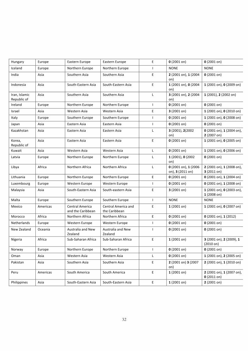
32

Hungary Europe EasternEurope EasternEurope E 0(2001on) 0(2001on)

Iceland Europe NorthernEurope NorthernEurope I NONE NONE

India Asia SouthernAsia SouthernAsia E 2(2001on),1(2004on)

0(2001on)

Indonesia Asia South-EasternAsia South-EasternAsia E 1(2001on),0(2004on)

1(2001on),0(2009on)

Iran,IslamicRepublicof

Asia SouthernAsia SouthernAsia L 3(2001on),2(2004on)

1(2001),2(2002on)

Ireland Europe NorthernEurope NorthernEurope I 0(2001on) 0(2001on)

Israel Asia WesternAsia WesternAsia E 3(2001on) 1(2001on),0(2010on)

Italy Europe SouthernEurope SouthernEurope I 0(2001on) 1(2001on),0(2008on)

Japan Asia EasternAsia EasternAsia I 0(2001on) 0(2001on)

Kazakhstan Asia EasternAsia EasternAsia L 3(2001),2(2002on)

0(2001on),1(2004on),2(2007on)

Korea,Republicof

Asia EasternAsia EasternAsia E 0(2001on) 1(2001on),0(2005on)

Kuwait Asia WesternAsia WesternAsia L 0(2001on) 1(2001on),0(2006on)

Latvia Europe NorthernEurope NorthernEurope L 1(2001),0(2002on)

0(2001on)

Libya Africa NorthernAfrica NorthernAfrica L 0(2001on),1(2006on),3(2011on)

2(2001on),1(2008on),3(2011on)

Lithuania Europe NorthernEurope NorthernEurope E 0(2001on) 0(2001on),1(2004on)

Luxembourg Europe WesternEurope WesternEurope I 0(2001on) 0(2001on),1(2008on)

Malaysia Asia South-EasternAsia South-easternAsia E 3(2001on) 1(2001on),0(2003on),1(2008on)

Malta Europe SouthernEurope SouthernEurope I NONE NONE

Mexico Americas CentralAmericaandtheCaribbean

CentralAmericaandtheCaribbean

E 1(2001on) 1(2001on),0(2007on)

Morocco Africa NorthernAfrica NorthernAfrica E 0(2001on) 0(2001on),1(2012)

Netherlands Europe WesternEurope WesternEurope I 0(2001on) 0(2001on)

NewZealand Oceania AustraliaandNewZealand

AustraliaandNewZealand

I 0(2001on) 0(2001on)

Nigeria Africa Sub-SaharanAfrica Sub-SaharanAfrica E 1(2001on) 3(2001on),2(2009),1(2010on)

Norway Europe NorthernEurope NorthernEurope I 0(2001on) 0(2001on)

Oman Asia WesternAsia WesternAsia L 0(2001on) 1(2001on),2(2005on)

Pakistan Asia SouthernAsia SouthernAsia E 2(2001on)3(2007on)

2(2001on),1(2010on)

Peru Americas SouthAmerica SouthAmerica E 1(2001on) 2(2001on),1(2007on),0(2011on)

Philippines Asia South-EasternAsia South-EasternAsia E 1(2001on) 2(2001on)

33

Poland Europe EasternEurope EasternEurope E 0(2001on) 0(2001on)

Portugal Europe SouthernEurope SouthernEurope I 0(2001on) 0(2001on)

Qatar Asia WesternAsia WesternAsia L 0(2001on) 1(2001on),2(2008on),1(2012)

Romania Europe EasternEurope EasternEurope L 2(2001on) 2(2001on),1(2004on),0(2006on)

RussianFederation

Europe EasternEurope EasternEurope E 0(2001on) 2(2001on),1(2006on),0(2010on)

SaudiArabia Asia WesternAsia WesternAsia L 3(2001on) 1(2001on),0(2005on),1(2008on)

Singapore Asia South-EasternAsia South-EasternAsia E 2(2001on) 0(2001on),1(2003),0(2004on)

Slovakia Europe EasternEurope EasternEurope E 1(2001on) 1(2001on),0(2003on)

Slovenia Europe SouthernEurope SouthernEurope E 0(2001on) 0(2001on)

SouthAfrica Africa Sub-SaharanAfrica Sub-SaharanAfrica E 2(2001on) 1(2001on),0(2004on),1(2012)

Spain Europe SouthernEurope SouthernEurope I 0(2001on) 0(2001on)

Sweden Europe NorthernEurope NorthernEurope I 0(2001on) 0(2001on)

Switzerland Europe WesternEurope WesternEurope I 1(2001on) 0(2001on)

TaiwanProvinceofChina

Asia EasternAsia EasternAsia E 0(2001on) 1(2001),0(2002on)

Thailand Asia South-EasternAsia South-EasternAsia E 0(2001on),1(2008on)

2(2001),1(2002on)

Tunisia Africa NorthernAfrica NorthernAfrica E 2(2001on),0(2011)

3(2001),2(2002on),1(2006on),2(2010on)

Turkey Asia WesternAsia WesternAsia E 3(2001on).2(2007),3(2008on),2(2011on)

0(2001on),1(2008on)

UnitedArabEmirates

Asia WesternAsia WesternAsia L 0(2001on) 2(2001),1(2002on),0(2004on)

UnitedKingdom

Europe NorthernEurope NorthernEurope I 0(2001on) 0(2001on)

UnitedStates Americas NorthernAmerica NorthernAmerica I 0(2001on) 0(2001on)

Venezuela,BolivarianRep.of

Americas SouthAmerica SouthAmerica E 2(2001on) 1(2001),2(2002on),1(2007on),2(2009on)3(2012)

VietNam Asia South-EasternAsia South-EasternAsia L 1(2001on) 0(2001on),1(2011on)

^E:emergingeconomies;I:industrialisedeconomies;L:lessdevelopedcountries^^Politicaleffectivenessandlegitimacyareclassifiedona4pointscalewherenofragility(0),lowfragility(1),mediumfragility(2),highfragility(3)

34

Table A2. 75 countries and the rest of the world: GDP, population, exports and FDI (percentage of the world)

GDP POPULATION EXPORTS FDI OUTSTOCKS

2001 97.5 82.3 92.3 72.3

2002 97.6 82.2 92.2 78.9

2003 97.6 82.1 92.4 77.1

2004 97.6 81.9 92.8 75.3

2005 97.5 81.8 92.6 71.6

2006 97.3 81.7 92.6 67.8

2007 97.1 81.5 91.9 68.5

2008 96.8 81.4 91.3 84.5

2009 96.9 81.2 91.0 81.5

2010 96.8 81.1 90.7 79.4

2011 96.7 80.9 90.2 81.6

2012 96.5 80.8 89.8 76.9

Source: authors elaborations on UNCTAD (2017) and World Bank (2017).

35

Table A3. Largest components dimension (LC) and isolated nodes (ISO) in FDI and Exports

FDI 2001*

2002

2003

2004

2005

2006

2007

2008*

2009

2010

2011

2012*

TV1 LC 75 75 75 75 75 75 75 75 75 75 75 75 ISO 0 0 0 0 0 0 0 0 0 0 0 0

TV2 LC 75 75 75 75 75 75 75 75 75 75 75 75 ISO 0 0 0 0 0 0 0 0 0 0 0 0

TV3 LC 75 75 75 75 75 75 75 75 75 75 75 75 ISO 0 0 0 0 0 0 0 0 0 0 0 0

TV4 LC 75 75 75 75 75 75 75 75 75 75 75 75 ISO 0 0 0 0 0 0 0 0 0 0 0 0

TV5 LC 75 75 75 75 75 75 75 75 75 75 75 75 ISO 0 0 0 0 0 0 0 0 0 0 0 0

TV6 LC 75 75 75 75 75 75 75 75 75 75 75 75 ISO 0 0 0 0 0 0 0 0 0 0 0 0

TV7 LC 75 74 74 74 74 75 75 75 75 75 75 75 ISO 0 1 1 1 1 0 0 0 0 0 0 0

TV8 LC 58 61 65 68 69 71 73 75 75 75 75 74 ISO 17 14 10 7 6 4 2 0 0 0 0 1

TV9^ LC 26 29 33 33 36 39 44 43 46 46 49 51 ISO 49 46 42 42 39 36 29 28 27 27 26 24

TV10 LC 7 8 8 10 9 10 13 11 13 14 14 15 ISO 66 65 65 63 64 63 60 62 58 57 57 56

EXP 2001*

2002

2003

2004

2005

2006

2007

2008*

2009

2010

2011

2012*

TV1 LC 75 75 75 75 75 75 75 75 75 75 75 75 ISO 0 0 0 0 0 0 0 0 0 0 0 0

TV2 LC 75 75 75 75 75 75 75 75 75 75 75 75 ISO 0 0 0 0 0 0 0 0 0 0 0 0

TV3 LC 75 75 75 75 75 75 75 75 75 75 75 75 ISO 0 0 0 0 0 0 0 0 0 0 0 0

TV4 LC 75 75 75 75 75 75 75 75 75 75 75 75 ISO 0 0 0 0 0 0 0 0 0 0 0 0

TV5 LC 75 75 75 75 75 75 75 75 75 75 75 75 ISO 0 0 0 0 0 0 0 0 0 0 0 0

TV6 LC 75 75 75 75 75 75 75 75 75 75 75 75 ISO 0 0 0 0 0 0 0 0 0 0 0 0

36

TV7 LC 75 75 75 75 75 75 75 75 75 75 75 75 ISO 0 0 0 0 0 0 0 0 0 0 0 0

TV8 LC 71 72 73 73 73 74 75 75 75 75 75 75 ISO 4 3 2 2 2 1 0 0 0 0 0 0

TV9^ LC 34 37 38 39 44 47 54 56 49 55 55 57 ISO 41 38 37 36 31 28 21 19 26 20 20 18

TV10 LC 4 4 4 6 6 6 9 9 6 7 10 10 ISO 71 71 71 69 69 66 66 66 66 65 65 65

* Figure 6 shows these values as percentages of total nodes; ^ TV9 is the threshold valueweselectedfortheanalyses

37

Table A3. Assortativity values (TV9 adiacency matrices)

geo_1 geo_2 geo_3 geo_dist economies polleg poleff

year Exports FDI Exports FDI Exports FDI Exports FDI Exports FDI Exports FDI Exports FDI

2001 0.511*** 0.220** 0.306*** 0.175*** 0.186*** 0.094 0.398*** 0.134* 0.076 0.149 -0.098** -0.055 -0.190*** -0.067*** 2002 0.485*** 0.204** 0.268*** 0.178*** 0.165*** 0.097* 0.381*** 0.164** 0.063 0.169 -0.103*** 0.023 -0.106 -0.073*** 2003 0.484*** 0.208*** 0.280*** 0.164*** 0.153*** 0.084* 0.365*** 0.170*** 0.097 0.198* -0.030 -0.013 -0.104* -0.088*** 2004 0.501*** 0.183** 0.283*** 0.192*** 0.150*** 0.103** 0.339*** 0.118** 0.133* 0.166 -0.001 -0.028 -0.051 -0.066*** 2005 0.463*** 0.216*** 0.249*** 0.167*** 0.130*** 0.089** 0.301*** 0.170*** 0.137** 0.158* -0.005 0.024 -0.041 -0.053*** 2006 0.461*** 0.217*** 0.270*** 0.169*** 0.133*** 0.085*** 0.281*** 0.144*** 0.157** 0.121* -0.018 0.019 -0.057 -0.065*** 2007 0.453*** 0.193*** 0.256*** 0.143*** 0.110*** 0.081** 0.276*** 0.136*** 0.183*** 0.066 -0.028 -0.035 -0.017 -0.076*** 2008 0.453*** 0.233*** 0.218*** 0.166*** 0.090*** 0.101*** 0.227*** 0.153*** 0.114** 0.142** -0.042 -0.037 -0.083** 0.027 2009 0.446*** 0.230*** 0.270*** 0.143*** 0.122*** 0.077** 0.270*** 0.141*** 0.189*** 0.125** -0.053 -0.010 -0.031 0.027 2010 0.459*** 0.247*** 0.243*** 0.138*** 0.095*** 0.071** 0.240*** 0.143*** 0.173*** 0.082 -0.020 -0.031 0.000 -0.025** 2011 0.462*** 0.257*** 0.238*** 0.147*** 0.104*** 0.072** 0.223*** 0.151*** 0.185*** 0.071 -0.015 -0.042 -0.017 -0.021** 2012 0.451*** 0.228*** 0.227*** 0.127*** 0.097*** 0.062** 0.217*** 0.101*** 0.173*** 0.064 -0.017 -0.048 -0.031 -0.027**

***, **, * significant respectively at 1%, 5%, 10%

38

Table A4. Assortativity values (raw adiacency matrices)

geo_1 geo_2 geo_3 geo_dist economies polleg poleff

year Exports FDI Exports FDI Exports FDI Exports FDI Exports FDI Exports FDI Exports FDI

2001 0.441*** 0.095 0.297*** 0.032 0.174*** -0.008 0.300*** 0.033 0.120** 0.240 -0.054 -0.044 -0.026 -0.021 2002 0.449*** 0.113 0.300*** 0.047 0.179*** 0.004 0.308*** 0.049 0.133** 0.231* -0.048 -0.045 -0.013 -0.011 2003 0.454*** 0.121 0.304*** 0.062 0.185*** 0.015 0.312*** 0.053 0.143** 0.231* -0.047 -0.049 -0.006 -0.013 2004 0.456*** 0.135 0.303*** 0.078 0.187*** 0.033 0.312*** 0.072 0.143** 0.241* -0.052* -0.054 -0.032 -0.026* 2005 0.453*** 0.150 0.295*** 0.091 0.185*** 0.043 0.302*** 0.085 0.140** 0.253* -0.048 -0.050 -0.030 -0.034*** 2006 0.451*** 0.156 0.289*** 0.103 0.181*** 0.054 0.298*** 0.101 0.141** 0.265* -0.043 -0.033 -0.022 -0.035** 2007 0.448*** 0.195* 0.287*** 0.124* 0.180*** 0.076 0.298*** 0.114 0.146*** 0.299* -0.039 0.009 0.000 -0.025* 2008 0.447*** 0.195** 0.278*** 0.142** 0.175*** 0.095 0.282*** 0.143** 0.134*** 0.302** -0.053* -0.021 0.000 -0.003 2009 0.441*** 0.197** 0.287*** 0.142** 0.176*** 0.096* 0.296*** 0.150** 0.144*** 0.290*** -0.058* -0.022 0.004 -0.012 2010 0.435*** 0.203** 0.284*** 0.140** 0.173*** 0.095* 0.288*** 0.153** 0.135** 0.288*** -0.062* -0.022 -0.001 -0.010 2011 0.436*** 0.207** 0.277*** 0.146** 0.167*** 0.102* 0.278*** 0.155** 0.134** 0.299*** -0.064* -0.024 -0.004 -0.007 2012 0.434*** 0.202** 0.278*** 0.131** 0.166*** 0.092 0.274*** 0.128** 0.136** 0.307*** -0.059* -0.015 0.001 0.004

***, **, * significant respectively at 1%, 5%, 10%

39

Figure A1. Exports and FDI distribution in 2001

a) Exports b) FDI

Similardistributionsapplyforallyears

40

Figure A2. Networks of Exports (2001, 2008, 2012) – TV9

Coloursidentifygeographicalareasaccordingtogeo_3

41

Figure A3. Networks of FDI (2001, 2008, 2012) – TV9

Coloursidentifygeographicalareasaccordingtogeo_3

Ultimi Contributi di Ricerca CRENoS I Paper sono disponibili in: Uhttp://www.crenos.itU

18/12 Gabriele Cardullo, Maurizio Conti, Giovanni Sulis, “Unions, Two-Tier Bargaining and Physical Capital Investment: Theory and Firm-Level Evidence from Italy”

18/11 Jing Guan, J.D. Tena, “Estimating the Effect of Physical Exercise on Juveniles’ Health Status and Subjective Well-Being in China”

18/10 Silvia Balia, Rinaldo Brau, Daniela Moro, “Hospital choice with high long-distance mobility”

18/09 Luca Deidda, Ettore Panetti, “Banks’ Liquidity Management and Financial Fragility”

18/08 Gerardo Marletto,�Cécile Sillig,�“Lost in mainstreaming?�Agrifood and urban mobility grassroots innovations with multiple pathways and outcomes”

18/07 Jing Guan, J.D. Tena, “Do Social Medical Insurance Schemes Improve Children’s Health in China?”

18/06 Carmenr Aina, Daniela Sonedda, “Investment in education and household consumption”

18/05 Maria Gabriella Campolo, Antonino Di Pino, Edoardo Otranto, “Reducing Bias in a Matching Estimation of Endogenous Treatment Effect”

18/04 William Addessi, Bianca Biagi, Maria Giovanna Brandano, “How tourist flows are affected by the introduction of the euro?”

18/03 Luc Bauwens, Edoardo Otranto, “Nonlinearities and Regimes in Conditional Correlations with Different Dynamics”

18/02 Massimiliano Bratti� Maurizio Conti, Giovanni Sulis, “Employment Protection, Temporary Contracts and Firm-provided Training: Evidence from Italy”

18/01 Luca De Benedictis, Vania Licio, Anna Maria Pinna, “The long-term effects of the historical Roman road network: Trade costs of Italian provinces”

17/11 Massimo Del Gatto, Carlo S. Mastinu, “A Huff model with heterogeneous retailers fits well in Southern Italy”

17/10 Sara Calligaris, Massimo Del Gatto, Fadi Hassan, Gianmarco I.P. Ottaviano, Fabiano Schivardi, “The Productivity Puzzle and Misallocation: an Italian Perspective”

17/09 Michele Battisti, Filippo Belloc. Massimo Del Gatto, “Technology-specific Production Functions”

17/08 Oliviero A. Carboni, Giuseppe Medda, “Do Investment and Innovation Boost Export? An Analysis on European Firms”

17/07 Edoardo Otranto, Massimo Mucciardi, “Clustering Space-Time Series: A Flexible STAR Approach”

17/06 Simone Franceschini, Gerardo Ettore Marletto, “The dynamics of social capital during public participation: new knowledge from an on-going monitoring”

17/05 Luca G. Deidda, Ettore Panetti, “Banks’ Liquidity Management and Systemic Risk”

17/04 Luca Frigau, Tiziana Medda, Vittorio Pelligra, “From the Field to the Lab�An Experiment on the Representativeness of Standard Laboratory Subjects”

17/03 William Addessi, Manuela Pulina, “Sectoral Composition of Consumption Expenditure: A Regional Analysis”

17/02 Claudio Detotto, Marta Meleddu, Marco Vannini, “Cultural identity and willingness to protect and preserve art”

17/01 Adriana Di Liberto, Laura Casula, “Teacher assessments versus standardized tests: is acting “girly” an advantage?”

www.crenos.it