Embed Size (px)
Citation preview
COMENIUS UNIVERSITY IN BRATISLAVA
Faculty of Mathematics, Physics and Informatics
Quadratic space-like Bézier curvesin three dimensional Minkowski space
Project of Dissertation Thesis
Advisor:
doc. RNDr. Pavel Chalmovianský, PhD.
Author:
RNDr. Barbora Pokorná
Bratislava 2012
Declaration
I hereby declare I wrote this Project of Dissertation Thesis by myself, only with
the help of referenced literature, under the supervision of my supervisor.
Bratislava, 27/02/2012 . . . . . . . . . . . . . . . . . . . . . . . . . . .
Barbora Pokorná

Acknowledgements
I would like to thank to my supervisor doc. RNDr. Pavel Chalmovianský, PhD.
for his great help, advices and supervising.
Abstract
This paper considers quadratic Bézier curves in three-dimensional Minkowski space.
We shall show the conditions for the control points A,C,B of the Bézier curve such
that the Bézier segment is space-like. For the middle control point C, we shall give
a geometrical interpretation of the feasibility condition. The work continues in the
spirit of the works [Gal10], [Pok11], [CP11]. We propose extensions of the topics
and methods used in the work for other classes of polynomial or rational curves.
Key words: Bézier curve, Minkowski space, space-like curve
Contents
1 Notation and Preliminaries 1
1.1 Minkowski space . . . . . . . . . . . . . . . . . . . . . . . . . . . . . 1
1.2 Bézier curves and surfaces . . . . . . . . . . . . . . . . . . . . . . . . 3
1.3 Extended Euclidean plane . . . . . . . . . . . . . . . . . . . . . . . . 7
1.4 Conic sections . . . . . . . . . . . . . . . . . . . . . . . . . . . . . . . 8
2 Space-like conditions for quadratic Bézier curves 10
2.1 Necessary conditions . . . . . . . . . . . . . . . . . . . . . . . . . . . 10
3 Set of admissible points of contact 13
3.1 Set of exterior points of contact . . . . . . . . . . . . . . . . . . . . . 15
3.2 Set of interior points of contact . . . . . . . . . . . . . . . . . . . . . 18
3.3 Set of points of contact . . . . . . . . . . . . . . . . . . . . . . . . . . 20
4 Boundary map 23
5 Area of admissible solutions 26
6 Examples 30
7 Conclusion 38
Project of Dissertation 39
Chapter 1
Notation and Preliminaries
In this chapter, we mention a basic definitions and properties of Bézier curves and
Minkowski space. The goal of this chapter is to clarify terms and relations, which we
use in this work. The following text is based on the works [Ber87b, Ber87a, DFN91,
Cha10].
1.1 Minkowski space
Pseudo-euclidean space, denoted by Rnp , n ∈ N, p ∈ N0 is an n−dimensional real
vector space with a regular quadratic form q : Rn → R, where q(x1, . . . , xn) =∑n−pi=1 x
2i −
∑nj=n−p+1 x
2j in certain basis. For p = 1, we call it Minkowski space, for
p = 0, we get Euclidean space. We use the notation x = (x1, . . . , xn) for vectors
in Rnp .
Let Mn,n(R) be the set of n × n matrices with real coefficients. We can write
the quadratic form q in a certain basis of Rn in the matrix form as q(x) = x>Qx,
where Q ∈ Mn,n(R) is symmetric and regular. A quadratic form has an associated
polar form P : Rn × Rn → R given by P (x, y) = x>Qy. Clearly, it is bilinear and
symmetric.
Since q(x) = P (x, x), the polar form plays a role of scalar product. Hence, we
call it pseudo-scalar product. We say, the vectors x, y ∈ Rnp are pseudo-orthogonal if
P (x, y) = 0.
1
Minkowski space Notation and Preliminaries
Although we consider vector space R, we get by standard construction an affine
space with a pseudo-Cartesian coordinate system S(O, x1, . . . , xn), where the axes
x1, . . . , xn are pseudo-orthogonal and O is the origin. We say, that the coordinate
axes x1, . . . , xn−p are space-like and the axes xn−p+1, . . . , xn are time-like. In the
following we work using such a setup.
Using the quadratic form, we classify the vectors in the pseudo-euclidean space.
We call the vector x ∈ Rnp space-like if q(x) > 0, time-like if q(x) < 0 and light-like
if q(x) = 0. All the vectors in q−1(0) are also called isotropic and they form a cone
Q. The set of all light-like vectors forms the isotropic cone Q of the corresponding
quadratic form. If a subspace F ⊂ Rnp consists of isotropic vectors, it is called
isotropic subspace. We say that the coordinate axes x1, . . . , xn−p are space-like and
the axes xn−p+1, . . . , xn are time-like.
A point x ∈ Rnp is space-like (time-like, light-like respectively) if its position
vector x = x − O is such. There are two possible ways, how to define space-like
curve (time-like and light-like respectively).
Definition 1. A differentiable curve p : I → Rnp is called space-like if the tangent
vector p(t) is space-like for each t ∈ I.
Definition 2 (Space-like curve). A curve p : I → Rnp is called space-like if it contains
only space-like points, i.e. vector p(t) = p(t)−O is space-like vector for every t ∈ I.
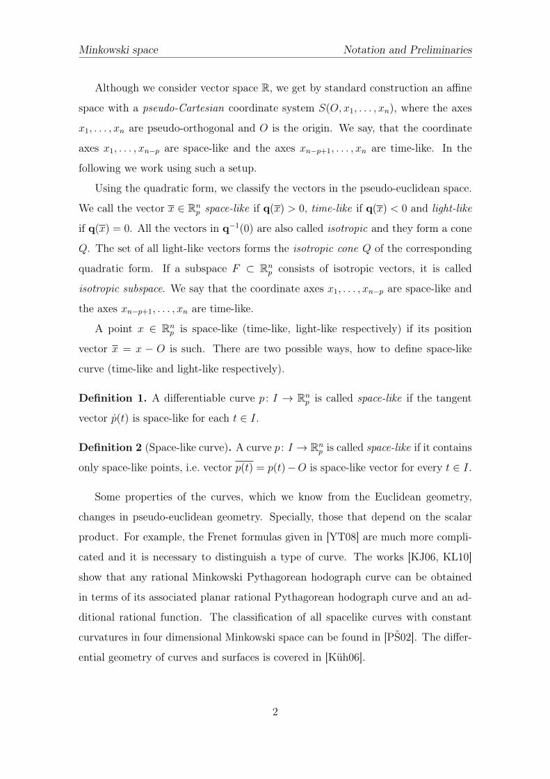
Some properties of the curves, which we know from the Euclidean geometry,
changes in pseudo-euclidean geometry. Specially, those that depend on the scalar
product. For example, the Frenet formulas given in [YT08] are much more compli-
cated and it is necessary to distinguish a type of curve. The works [KJ06, KL10]
show that any rational Minkowski Pythagorean hodograph curve can be obtained
in terms of its associated planar rational Pythagorean hodograph curve and an ad-
ditional rational function. The classification of all spacelike curves with constant
curvatures in four dimensional Minkowski space can be found in [PŠ02]. The differ-
ential geometry of curves and surfaces is covered in [Küh06].
2
Bézier curves and surfaces Notation and Preliminaries
b0
b1
b2
b3
b(t)
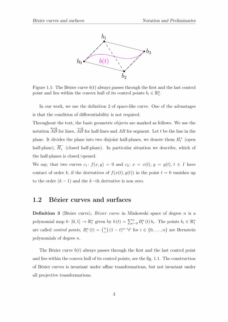
Figure 1.1: The Bézier curve b(t) always passes through the first and the last controlpoint and lies within the convex hull of its control points bi ∈ Rn
1 .
In our work, we use the definition 2 of space-like curve. One of the advantages
is that the condition of differentiability is not required.
Throughout the text, the basic geometric objects are marked as follows. We use the
notation←→AB for lines,
−→AB for half-lines and AB for segment. Let t be the line in the
plane. It divides the plane into two disjoint half-planes, we denote them H+t (open
half-plane), H−t (closed half-plane). In particular situation we describe, which of
the half-planes is closed/opened.
We say, that two curves c1 : f(x, y) = 0 and c2 : x = x(t), y = y(t), t ∈ I have
contact of order k, if the derivatives of f(x(t), y(t)) in the point t = 0 vanishes up
to the order (k − 1) and the k−th derivative is non zero.
1.2 Bézier curves and surfaces
Definition 3 (Bézier curve). Bézier curve in Minkowski space of degree n is a
polynomial map b : [0, 1] → Rn1 given by b (t) =
∑ni=0B
ni (t) bi. The points bi ∈ Rn
1
are called control points, Bni (t) =
(ni
)(1 − t)n−iti for i ∈ {0, . . . , n} are Bernstein
polynomials of degree n.
The Bézier curve b(t) always passes through the first and the last control point
and lies within the convex hull of its control points, see the fig. 1.1. The construction
of Bézier curves is invariant under affine transformations, but not invariant under
all projective transformations.
3
Bézier curves and surfaces Notation and Preliminaries
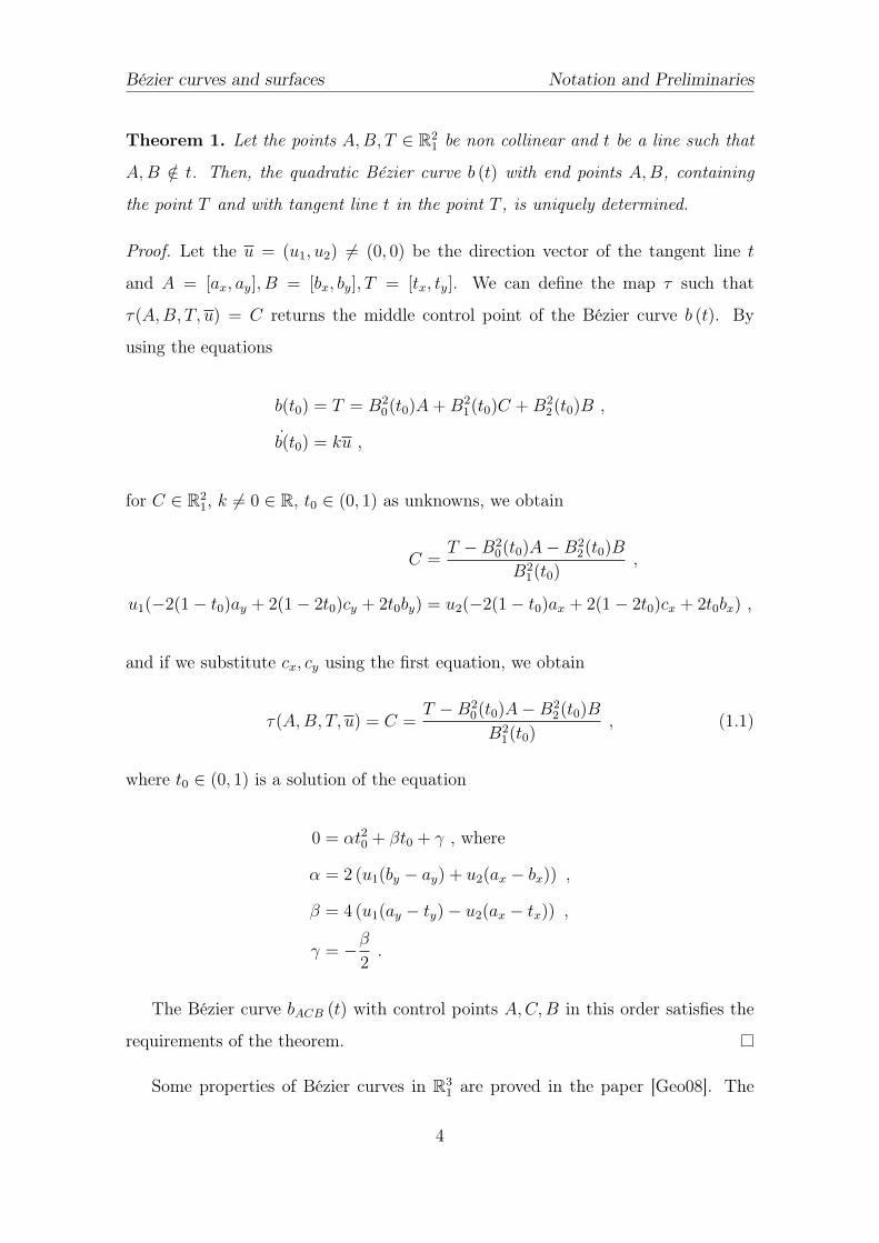
Theorem 1. Let the points A,B, T ∈ R21 be non collinear and t be a line such that
A,B /∈ t. Then, the quadratic Bézier curve b (t) with end points A,B, containing
the point T and with tangent line t in the point T , is uniquely determined.
Proof. Let the u = (u1, u2) 6= (0, 0) be the direction vector of the tangent line t
and A = [ax, ay], B = [bx, by], T = [tx, ty]. We can define the map τ such that
τ(A,B, T, u) = C returns the middle control point of the Bézier curve b (t). By
using the equations
b(t0) = T = B20(t0)A+B2
1(t0)C +B22(t0)B ,
b(t0) = ku ,
for C ∈ R21, k 6= 0 ∈ R, t0 ∈ (0, 1) as unknowns, we obtain
C =T −B2
0(t0)A−B22(t0)B
B21(t0)
,
u1(−2(1− t0)ay + 2(1− 2t0)cy + 2t0by) = u2(−2(1− t0)ax + 2(1− 2t0)cx + 2t0bx) ,
and if we substitute cx, cy using the first equation, we obtain
τ(A,B, T, u) = C =T −B2
0(t0)A−B22(t0)B
B21(t0)
, (1.1)
where t0 ∈ (0, 1) is a solution of the equation
0 = αt20 + βt0 + γ , where
α = 2 (u1(by − ay) + u2(ax − bx)) ,
β = 4 (u1(ay − ty)− u2(ax − tx)) ,
γ = −β2.
The Bézier curve bACB (t) with control points A,C,B in this order satisfies the
requirements of the theorem.
Some properties of Bézier curves in R31 are proved in the paper [Geo08]. The
4
Bézier curves and surfaces Notation and Preliminaries
author use the definition 1 of space-like curves. Let us mention some of them.
Theorem 2. Let bM (t) =∑n
i=0Bni (t) bi be the Bézier curve in Minkowski space.
If the vectors 4bi = bi+1 − bi for i ∈ {0, . . . , n− 1} are space-like, then the curve
bM (t) is space-like.
Theorem 3. Let πi : R31 → R, where i = 1, 2, 3 is such that for x = (x1, x2, x3) ∈ R3
1
holds πi (x) = xi. Let bM (t) is Bézier curve in R31. If π1 (4bi) = π2 (4bi) or
π1 (4bi) = π3 (4bi) for i ∈ {0, . . . , n− 1}, then bM (t) is space-like and non regular.
Theorem 4. If the Bézier curve bM (t) is space-like, then the vectors 4b0 = b1− b0and 4bn−1 = bn − bn−1 are space-like.
Note 1. The space-like Bézier curve bM (t) with control points b0, . . . , bn, where
n > 3 is closed, if b0 = bn and b0 is in the middle of the segment [b1, bn−1].
Definition 4 (Pseudo-vector product). The pseudo-vector product is bilinear func-
tion θ : R31 × R3
1 → R31 such that for given x = (x1, x2, x3) , y = (y1, y2, y3) ∈ R3
1 is
θ (x, y) = x× y = (x2y3 − x3y2, x3y1 − x1y3,−x1y2 + x2y1).
Theorem 5. Let bM (t) be space-like Bézier curve. Let us define the functions
Q1 (t) = 〈b′M (t) , b′M (t)〉 ,
Q2 (t) = 〈b′M (t)× b′′M (t) , b′M (t)× b′′M (t)〉 ,
Q3 (t) = 〈b′M (t)× b′′M (t) , b′′′M (t)〉 .
If bM (t) is regular for some t0 ∈ [0, 1], then for the curvature and torsion of Bézier
curve in the point t0 holds
κ (t0) =
√|Q2 (t0)|(√Q1 (t0)
)3 ,
τ (t0) =Q3 (t0)
Q2 (t0).
There are also articles about the surfaces, which can be expressed in Bézier form.
The properties of space-like Bézier surfaces in R31 are proved in the papers [Geo09]
5
Bézier curves and surfaces Notation and Preliminaries
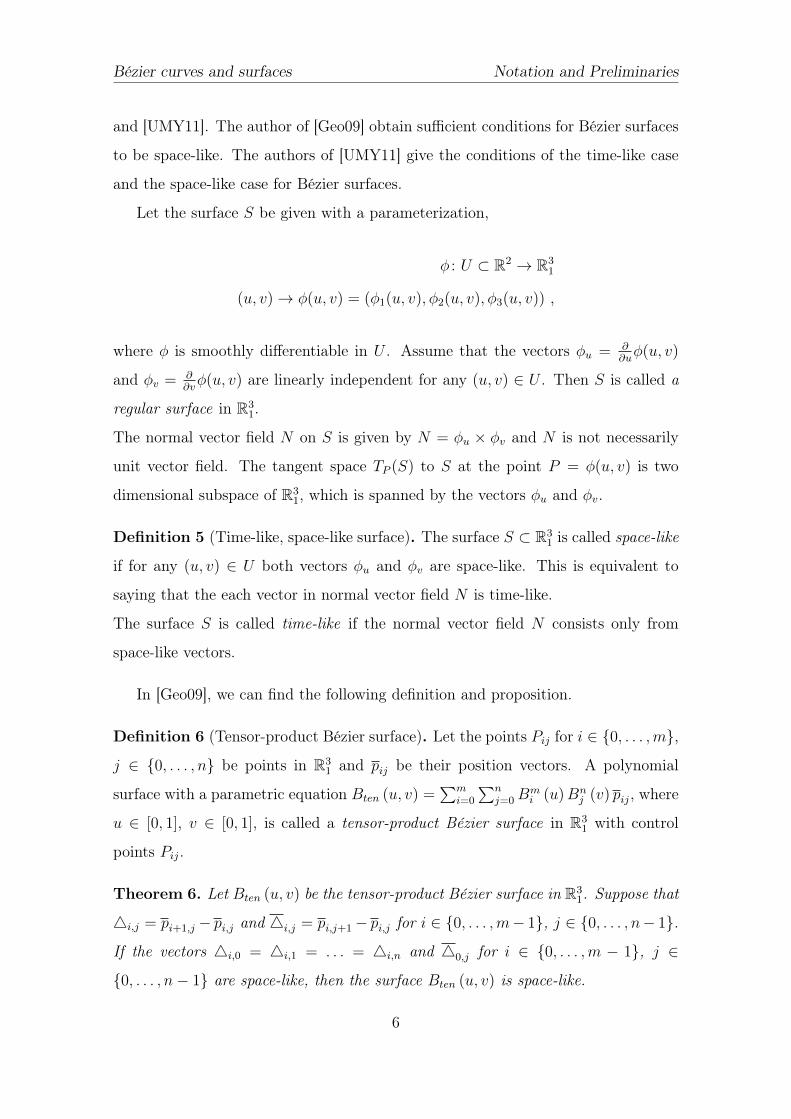
and [UMY11]. The author of [Geo09] obtain sufficient conditions for Bézier surfaces
to be space-like. The authors of [UMY11] give the conditions of the time-like case
and the space-like case for Bézier surfaces.
Let the surface S be given with a parameterization,
φ : U ⊂ R2 → R31
(u, v)→ φ(u, v) = (φ1(u, v), φ2(u, v), φ3(u, v)) ,
where φ is smoothly differentiable in U . Assume that the vectors φu = ∂∂uφ(u, v)
and φv = ∂∂vφ(u, v) are linearly independent for any (u, v) ∈ U . Then S is called a
regular surface in R31.
The normal vector field N on S is given by N = φu × φv and N is not necessarily
unit vector field. The tangent space TP (S) to S at the point P = φ(u, v) is two
dimensional subspace of R31, which is spanned by the vectors φu and φv.
Definition 5 (Time-like, space-like surface). The surface S ⊂ R31 is called space-like
if for any (u, v) ∈ U both vectors φu and φv are space-like. This is equivalent to
saying that the each vector in normal vector field N is time-like.
The surface S is called time-like if the normal vector field N consists only from
space-like vectors.
In [Geo09], we can find the following definition and proposition.
Definition 6 (Tensor-product Bézier surface). Let the points Pij for i ∈ {0, . . . ,m},
j ∈ {0, . . . , n} be points in R31 and pij be their position vectors. A polynomial
surface with a parametric equation Bten (u, v) =∑m
i=0∑n
j=0Bmi (u)Bn
j (v) pij, where
u ∈ [0, 1], v ∈ [0, 1], is called a tensor-product Bézier surface in R31 with control
points Pij.
Theorem 6. Let Bten (u, v) be the tensor-product Bézier surface in R31. Suppose that
4i,j = pi+1,j − pi,j and 4i,j = pi,j+1− pi,j for i ∈ {0, . . . ,m− 1}, j ∈ {0, . . . , n− 1}.
If the vectors 4i,0 = 4i,1 = . . . = 4i,n and 40,j for i ∈ {0, . . . ,m − 1}, j ∈
{0, . . . , n− 1} are space-like, then the surface Bten (u, v) is space-like.
6
Extended Euclidean plane Notation and Preliminaries
The paper [UMY11] shows that type of surface depends on the corresponding
control net of the surface.
The polar form P in R31 ⊃ S induces the polar form denoted by PP in each tangent
plane TP (S) of the smooth surface S. For any x, y ∈ TP (S) ⊂ R31 holds P (x, y) =
PP (x, y). The symmetric, bilinear polar form PP has an associated quadratic form
IP : TP (S)→ R given by IP (w) = PP (w,w). The quadratic form IP is called the first
fundamental form of the surface S in the point P ∈ S. The first fundamental form of
the surface S can be expressed in the basis {φu, φv} as IP (w) = Edu2+Fdudv+Gdv2,
where E(u, v) = PP (φu, φu), F (u, v) = PP (φu, φv), G(u, v) = PP (φv, φv) are the
differentiable coefficients. In the paper, the first fundamental form coefficients are
derived in terms of coordinates of control points of the surface, we denote them
EB, FB, GB. Then, the next proposition holds.
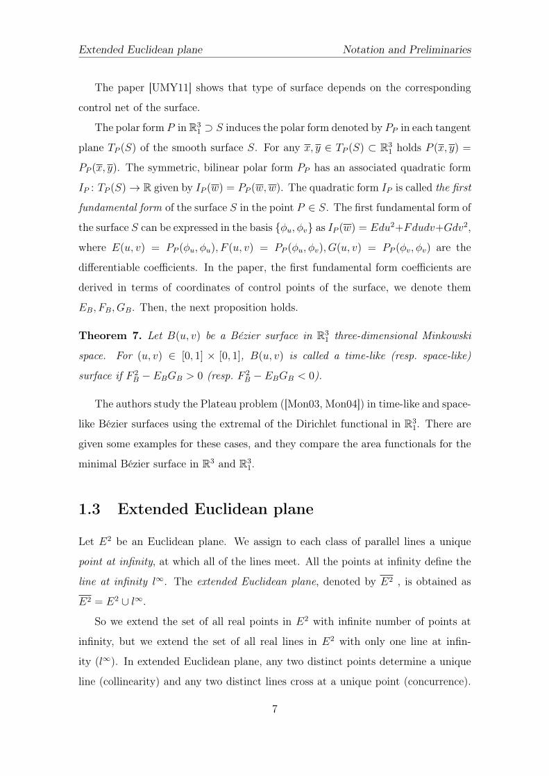
Theorem 7. Let B(u, v) be a Bézier surface in R31 three-dimensional Minkowski
space. For (u, v) ∈ [0, 1] × [0, 1], B(u, v) is called a time-like (resp. space-like)
surface if F 2B − EBGB > 0 (resp. F 2
B − EBGB < 0).
The authors study the Plateau problem ([Mon03, Mon04]) in time-like and space-
like Bézier surfaces using the extremal of the Dirichlet functional in R31. There are
given some examples for these cases, and they compare the area functionals for the
minimal Bézier surface in R3 and R31.
1.3 Extended Euclidean plane
Let E2 be an Euclidean plane. We assign to each class of parallel lines a unique
point at infinity, at which all of the lines meet. All the points at infinity define the
line at infinity l∞. The extended Euclidean plane, denoted by E2 , is obtained as
E2 = E2 ∪ l∞.
So we extend the set of all real points in E2 with infinite number of points at
infinity, but we extend the set of all real lines in E2 with only one line at infin-
ity (l∞). In extended Euclidean plane, any two distinct points determine a unique
line (collinearity) and any two distinct lines cross at a unique point (concurrence).
7
Conic sections Notation and Preliminaries
These statements are dual, which means they are formed by changing points to lines
and collinearity to concurrence.
Let S(O, e1, e2) be an affine coordinate system in E2. Then each point at infinity
a∞ ∈ E2 corresponding to real line a has homogeneous coordinates [x1, x2, 0], where
x1, x2 ∈ R and (x1, x2) 6= (0, 0) is direction vector of the real line a. Each real point
A belongs to real line a has homogeneous coordinates [x1, x2, x3], where x3 6= 0 and
[x1x3, x2x3
] are its affine coordinates. Hence, each point in E2 (real or at infinity) has
an infinite number of triplet of homogeneous coordinates.
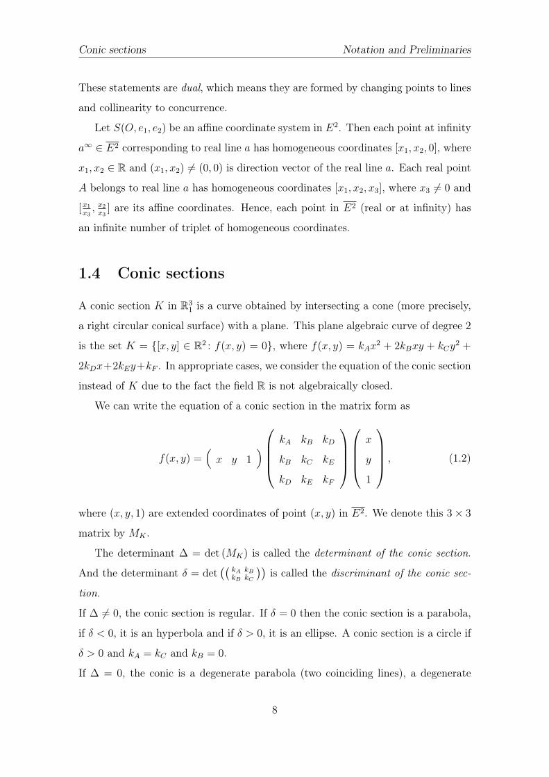
1.4 Conic sections
A conic section K in R31 is a curve obtained by intersecting a cone (more precisely,
a right circular conical surface) with a plane. This plane algebraic curve of degree 2
is the set K = {[x, y] ∈ R2 : f(x, y) = 0}, where f(x, y) = kAx2 + 2kBxy + kCy
2 +
2kDx+2kEy+kF . In appropriate cases, we consider the equation of the conic section
instead of K due to the fact the field R is not algebraically closed.
We can write the equation of a conic section in the matrix form as
f(x, y) =(x y 1
)kA kB kD
kB kC kE
kD kE kF
x
y
1
, (1.2)
where (x, y, 1) are extended coordinates of point (x, y) in E2. We denote this 3× 3
matrix by MK .
The determinant ∆ = det (MK) is called the determinant of the conic section.
And the determinant δ = det((
kA kBkB kC
))is called the discriminant of the conic sec-
tion.
If ∆ 6= 0, the conic section is regular. If δ = 0 then the conic section is a parabola,
if δ < 0, it is an hyperbola and if δ > 0, it is an ellipse. A conic section is a circle if
δ > 0 and kA = kC and kB = 0.
If ∆ = 0, the conic is a degenerate parabola (two coinciding lines), a degenerate
8
Conic sections Notation and Preliminaries
ellipse (a point ellipse), or a degenerate hyperbola (two intersecting lines).
In the extended Euclidean plane, it is necessary to homogenize the equation (1.2)
by replacing (x, y, 1) with (x, y, z). We obtain the conic section K = {[x, y, z] ∈
R2 : f(x, y, z) = 0} in homogeneous coordinates.
From each pointX ∈ R2 lying outside the regular conic section, one can construct
two tangent lines to regular K. The corresponding points of contact may be either
real or at infinity. In the case of point at infinity of the contact, the conic section K
is hyperbola and the tangent line is the asymptote a. We denote by a∞ the point of
contact at infinity, see fig. 3.3. We denote the set of all tangent lines to K by TK .
We denote by ∇f(x0, y0) the gradient of K in the point [x0, y0] ∈ K.
9
Chapter 2
Space-like conditions for quadratic
Bézier curves
Let us consider a Minkowski space R31 and a quadratic Bézier curve with control
points A,C,B in this order, denoted by bACB (t). We find the necessary and sufficient
condition for the control points A,B. Then, we fix them and we are looking for the
set of all such points C that the Bézier curve bACB (t) is space-like.
2.1 Necessary conditions for the end points
In order a Bézier curve to be space-like, each of its points have to be space-like.
Let the points A = [a1, a2, a3] and B = [b1, b2, b3] be fixed. Since Bézier curve
interpolates its endpoints, we have necessary and sufficient conditions
a21 + a22 − a23 > 0 , (2.1)
b21 + b22 − b23 > 0 . (2.2)
A generic quadratic Bézier curve is a part of a parabola (see the fig. 2.2), so
it lies in the plane ρ ⊂ R31. Since the given points A,B ∈ ρ, the construction of
the plane ρ has several degrees of freedom depending on their positions. By using
10
Necessary conditions Space-like conditions for quadratic Bézier curves
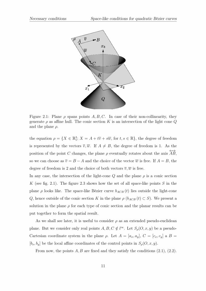
Figure 2.1: Plane ρ spans points A,B,C. In case of their non-collinearity, theygenerate ρ as affine hull. The conic section K is an intersection of the light cone Qand the plane ρ.
the equation ρ = {X ∈ R31; X = A + tv + sw, for t, s ∈ R}, the degree of freedom
is represented by the vectors v, w. If A 6= B, the degree of freedom is 1. As the
position of the point C changes, the plane ρ eventually rotates about the axis←→AB,
so we can choose as v = B−A and the choice of the vector w is free. If A = B, the
degree of freedom is 2 and the choice of both vectors v, w is free.
In any case, the intersection of the light-cone Q and the plane ρ is a conic section
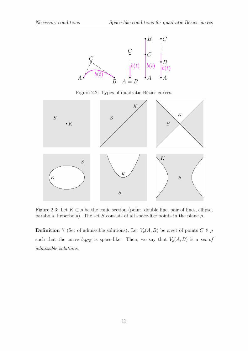
K (see fig. 2.1). The figure 2.3 shows how the set of all space-like points S in the
plane ρ looks like. The space-like Bézier curve bACB (t) lies outside the light-cone
Q, hence outside of the conic section K in the plane ρ (bACB (t) ⊂ S). We present a
solution in the plane ρ for each type of conic section and the planar results can be
put together to form the spatial result.
As we shall see later, it is useful to consider ρ as an extended pseudo-euclidean
plane. But we consider only real points A,B,C /∈ l∞. Let Sρ(O, x, y) be a pseudo-
Cartesian coordinate system in the plane ρ. Let A = [ax, ay], C = [cx, cy] a B =
[bx, by] be the local affine coordinates of the control points in Sρ(O, x, y).
From now, the points A,B are fixed and they satisfy the conditions (2.1), (2.2).
11
Necessary conditions Space-like conditions for quadratic Bézier curves
b(t)A
C
B
b(t)
A = B
C
b(t)
A
C
B
b(t)
A
C
B
Figure 2.2: Types of quadratic Bézier curves.
KS
K
SK
S
S
KK
S
S
K
Figure 2.3: Let K ⊂ ρ be the conic section (point, double line, pair of lines, ellipse,parabola, hyperbola). The set S consists of all space-like points in the plane ρ.
Definition 7 (Set of admissible solutions). Let Vρ(A,B) be a set of points C ∈ ρ
such that the curve bACB is space-like. Then, we say that Vρ(A,B) is a set of
admissible solutions.
12
Chapter 3
Set of admissible points of contact
In this chapter, we study for the given points A,B all Bézier curves bACB such that
common points of the curve bACB and conic section K are only the points of their
contact. It is natural, because a "boundary" between the situation that two curves
have no common points and the situation that one curve intersects the other curve
is, that they touch each other.
Definition 8 (Set of points of contact). We say that the set D ⊂ K is the set of
points of contact between K and the set of all bACB if for any point X = [x0, y0] ∈ D
there is a point C such that bACB(t) ∩K = M , where X ∈ M is a point of contact
of order 2 and the set M contains only points of contact of order 2 between bACB(t)
and K.
Note 2. The set M contains at most two points, since two different quadratic
curves may have at most two common points of contact of order 2 (Bézout theorem
[Kun05]). If we will mark a point by letter T , we mean a point of the contact.
Definition 9 (Double contact). We say that bACB has double contact, if it has
with K exactly two points of contact of order 2 (i.e. the set M contains exactly
two points). We denote the middle control point of the Bézier curve Cu. If K is
regular conic section, we denote the touch points by the letter Ui (see the fig. 6.4).
If K is singular conic section, we denote the touch points by the letter Si (see the
fig. 6.2(b)).
13
Set of admissible points of contact
A B
C
Tt
H+t
H−t
K
bACB
A B
C
T t
K
bACB
A B
CT t
K
bACB
X
(a) (b) (c)
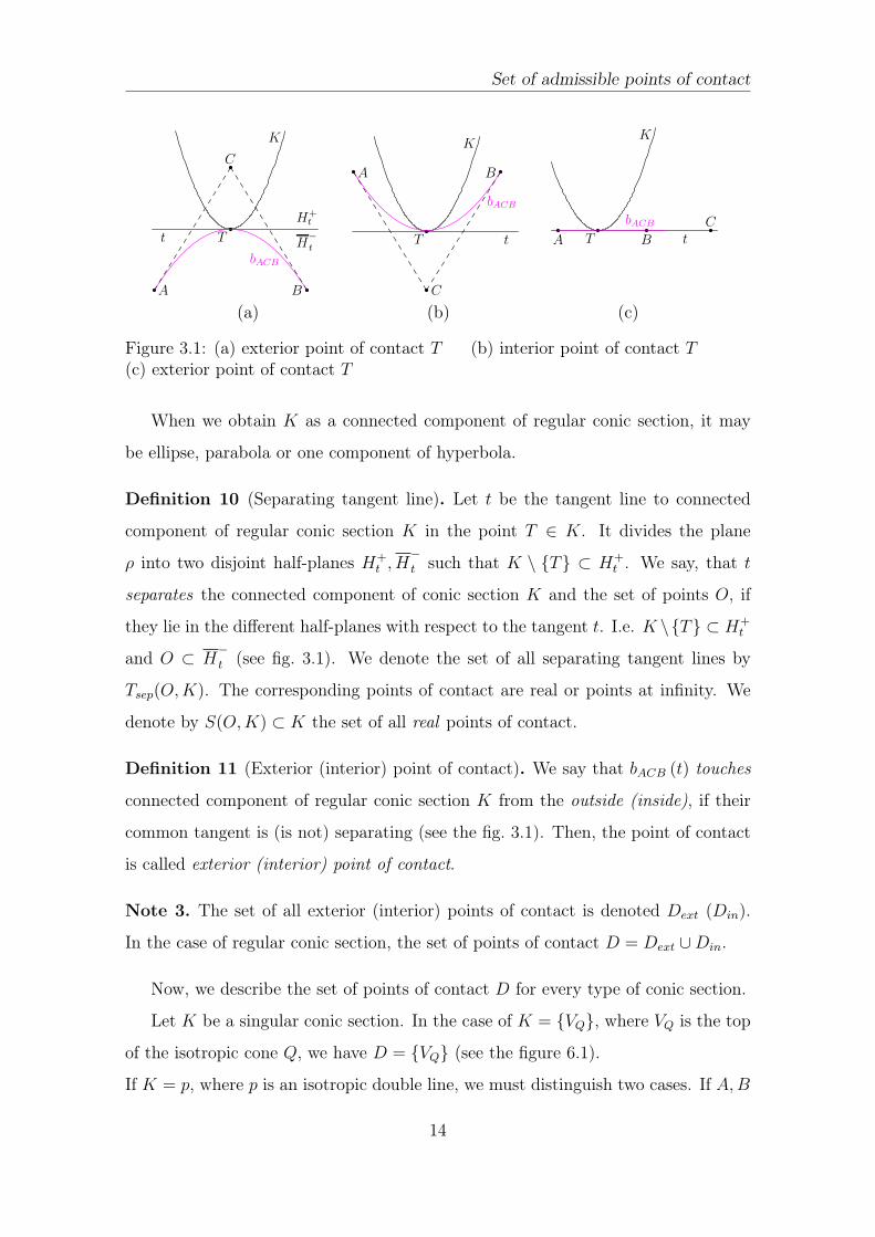
Figure 3.1: (a) exterior point of contact T (b) interior point of contact T(c) exterior point of contact T
When we obtain K as a connected component of regular conic section, it may
be ellipse, parabola or one component of hyperbola.
Definition 10 (Separating tangent line). Let t be the tangent line to connected
component of regular conic section K in the point T ∈ K. It divides the plane
ρ into two disjoint half-planes H+t , H
−t such that K \ {T} ⊂ H+
t . We say, that t
separates the connected component of conic section K and the set of points O, if
they lie in the different half-planes with respect to the tangent t. I.e. K \{T} ⊂ H+t
and O ⊂ H−t (see fig. 3.1). We denote the set of all separating tangent lines by
Tsep(O,K). The corresponding points of contact are real or points at infinity. We
denote by S(O,K) ⊂ K the set of all real points of contact.
Definition 11 (Exterior (interior) point of contact). We say that bACB (t) touches
connected component of regular conic section K from the outside (inside), if their
common tangent is (is not) separating (see the fig. 3.1). Then, the point of contact
is called exterior (interior) point of contact.
Note 3. The set of all exterior (interior) points of contact is denoted Dext (Din).
In the case of regular conic section, the set of points of contact D = Dext ∪Din.
Now, we describe the set of points of contact D for every type of conic section.
Let K be a singular conic section. In the case of K = {VQ}, where VQ is the top
of the isotropic cone Q, we have D = {VQ} (see the figure 6.1).
If K = p, where p is an isotropic double line, we must distinguish two cases. If A,B
14
Set of exterior points of contact Set of admissible points of contact
lie in the opposite half-planes generated by the line p, we have D = ∅. If A,B lie in
the same half-plane, the set of points of contact D = p (see the figure 6.2(a)).
The last singular case is K = p ∪ r, where p, r are pair of distinct isotropic lines.
Then, there are two space-like regions in the plane ρ. If A,B lie in the different
regions, there is no space-like Bézier curve bACB. Let A,B lie in the same region,
which is determined by two half-lines−−→VQP ⊂ p and
−−→VQR ⊂ r. Let Sp ∈ p and Sr ∈ r
are the points of contact of the Bézier curve bACuB, i.e. bACuB ∩ K = {Sp, Sr} is
double contact. Then D =−−→SpP ∪
−−→SrR (see the figure 6.2(b)). The special case is
Sp = Sr = VQ.
Let K be a regular conic section. From each space-like point X ∈ ρ, one can
construct two tangent lines to K.
3.1 Set of exterior points of contact
Now, we describe the set Tsep(AB,K) for the given A,B, because the corresponding
real points of contact S(AB,K) form the set Dext.
Let K be a regular conic section, but not hyperbola. Let t1A, t2A, t1B, t2B be the
tangent lines from the points A,B to K and the points T1A, T2A, T1B, T2B ∈ K be
the corresponding real points of contact. The points T1A, T2A split the conic section
K to some arcs. We denote_
T1AT2A the arc_
T1AT2A⊂ 4AT1AT2A. Similarly, for
points B, T1B, T2B we get_
T1BT2B. In order A (B) to be separated from K, the point
T ∈_
T1AT2A (T ∈_
T1BT2B). So, the set S(A,K) =_
T1AT2A and S(B,K) =_
T1BT2B (see
fig. 3.2).
If K = K1 ∪K2 is hyperbola, where K1, K2 are connected components of K, we
need to consider each of them separately. Let a1, a2 be the asymptotes of hyperbola.
It may not hold that all the points of contact T1A, T2A, T1B, T2B ∈ {K1 ∪ a∞1 ∪ a∞2 }.
Let both T1A, T2A ∈ K2. If t ∈ TK1 , then also t ∈ Tsep(A,K1). Hence, if we an-
alyze the case of K1, then S(A,K1) =_
a∞1 a∞2 = K1 and Tsep(A,K1) = TK1 . Let
T1A ∈ {K1 ∪ a∞1 ∪ a∞2 } and T2A ∈ K2. Since the asymptote a1 ∈ Tsep(A,K1), the set
15
Set of exterior points of contact Set of admissible points of contact
A
K
t1A
t2A
T1A
T2A
t
T
H−t H+
tA
B
t1B
t2B
t1A
t2A
T1B
T2B
T1A
T2A
K
(a) (b)
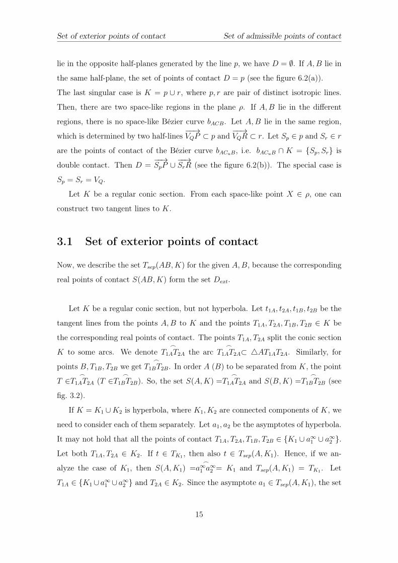
Figure 3.2: (a) the arc S(A,K) =_
T1AT2A⊂ 4AT1AT2A determines all tangent linesTsep(A,K) that separate A and K(b) the arc S(A,K)∩S(B,K) determines all tangent lines Tsep(AB,K) that separateAB and K
S(A,K1) =_
T1Aa∞1 ⊂ K1 define the set Tsep(A,K1). Similarly, for the point B or K2.
For the corresponding illustration see fig. 3.3.
Lemma 8 (Separating tangent line). Let A,B be space-like points and K be a
connected component of regular conic section. Let t ∈ TK and the point T ∈ K be
its point of contact. The tangent line t ∈ Tsep(AB,K) if and only if T ∈ S(A,K) ∩
S(B,K) (see fig. 3.2 for the case of ellipse).
Proof. Sufficient condition. If the tangent line t is separating, then the points A,B
and the conic section K are separated. In order A (B) to be separated from K, the
point T ∈ S(A,K) (T ∈ S(B,K)). Since A and B should be separated simultane-
ously, T must belong to the intersection of these two arcs.
Necessary condition. Let a point T ∈ S(A,K) ∩ S(B,K) and K \ {T} ⊂ H+t .
Because the point T ∈ S(A,K) we have the point A ∈ H−t . Also the point T ∈
S(B,K), so the point B ∈ H−t . Therefore, entire segment AB ⊂ H
−t due to
convexity of H−t .
Theorem 9 (Set of exterior points of contact). Let A,B be space-like points and K
be a regular connected conic section. The set of exterior points of contact Dext 6= ∅
if and only if the segment AB ∩K = ∅ or AB ∩K = {T0}.
16
Set of exterior points of contact Set of admissible points of contact
K2K1
A
B
T2A
a∞1
T1Aa1a2
K2K1
A
B
T1BT2B
a∞1
a1 a2
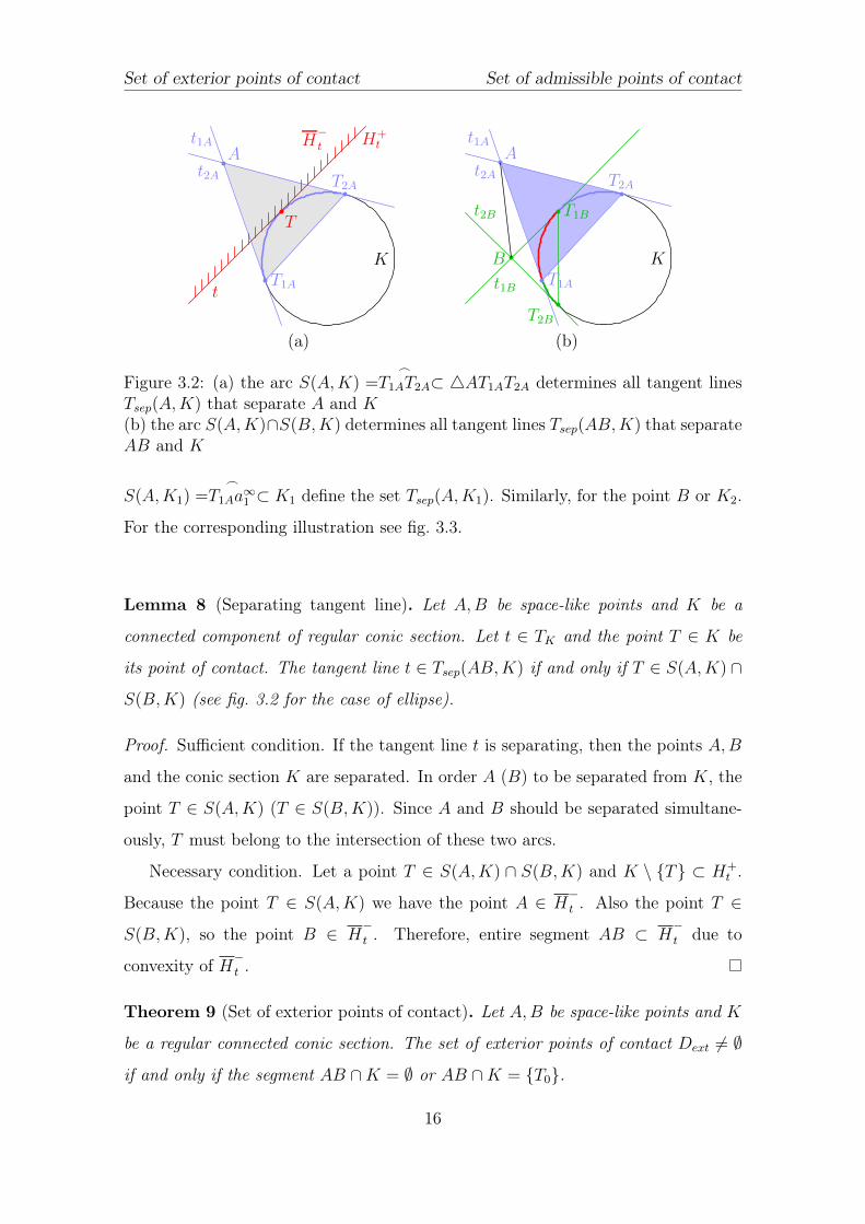
(a) (b)
Figure 3.3: (a) Let us find, how the set Tsep(A,K1) looks like. The point T1A =a∞2 ∈ {K1 ∪ a∞1 ∪ a∞2 }. Because T2A ∈ K2, we have to "replace it" by a∞1 ∈{K1 ∪ a∞1 ∪ a∞2 }, where the asymptote a1 ∈ Tsep(A,K1). The set of separatingtangent lines Tsep(A,K1) is determined by the arc of corresponding points of contact
S(A,K1) =_
T1Aa∞1 ⊂ 4AT1Aa∞1 . Since T1A = a∞2 , we have S(A,K1) = K1.
(b) If we are seeking the set Tsep(B,K1), we have to "replace" the T2B ∈ K2 bya∞1 ∈ {K1 ∪ a∞1 ∪ a∞2 } (not by a∞2 , because a2 /∈ Tsep(B,K1)). The set Tsep(B,K1)
is determined by the arc of corresponding points of contact S(B,K1) =_
T1Ba∞1 ⊂
4BT1Ba∞1 .
The set Dext consists of an arc S(A,K) ∩ S(B,K) on K. The end point of the
arc T ∈ Dext if and only if its corresponding tangent line t to K contains both the
end points of the curve bACB(t), the control points A and B.
Note 4. As we said, we consider the hyperbola as two separate subsets K1, K2 of a
conic section. Therefore, there could be two continuous arcs D1ext, D
2ext, one on each
component K1, K2. Then Dext = D1ext ∪D2
ext.
Proof. Sufficient condition. Let AB ∩K = {X1, X2}. Then S(A,K)∩ S(B,K) = ∅
so there exists no separating tangent line t ∈ Tsep(AB,K). Hence, for any Bézier
curve bACB there exists no separating tangent line Tsep(bACB, K). Consequently the
set Dext = ∅.
Necessary condition. At first, let AB∩K = ∅. Then S(A,K)∩S(B,K) 6= ∅. Let
t ∈ TK and the point T ∈ K be its corresponding point of contact. Using the theo-
rem 1, the quadratic curve bACB is uniquely determined by the points A,B, T and by
the tangent line t. If T /∈ S(A,K)∩S(B,K), then the tangent line t /∈ Tsep(AB,K),
t /∈ Tsep(bACB, K) and T /∈ Dext. On the other hand, because quadratic Bézier
17
Set of interior points of contact Set of admissible points of contact
curve is a convex curve, each of its tangent line defines the supporting half-plane
to the curve. If t ∈ Tsep(A,K) and t ∈ Tsep(B,K), then t ∈ Tsep(bACB, K). So,
for every T ∈ S(A,K) ∩ S(B,K) holds that t ∈ Tsep(bACB, K). Hence, we have
Dext = S(A,K) ∩ S(B,K) 6= ∅.
Now, let AB ∩ K = {T0}, then S(A,K) ∩ S(B,K) = {T0}. So there is only one
separating tangent line t0 ∈ Tsep(AB,K) and Dext = {T0} 6= ∅.
Without loss of generality, let Bézier curve bACB is determined by the points
A,B, T1A and tangent line t1A to K and T1A ∈ Dext. It holds if and only if the
tangent line to bACB in the end point A is the same as tangent line t1A. It holds if
and only if the Bézier curve is a segment and the points A,B, T1A ∈ t1A are collinear.
Note: if for both end points T1, T2 of the arc Dext holds that T1, T2 ∈ Dext, then
A = B.
Note 5. We denote by De the set of all T ∈ Dext such that the corresponding
tangent line t to K at T contains both control points A,B.
3.2 Set of interior points of contact
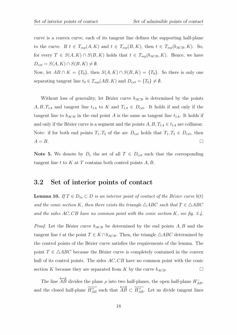
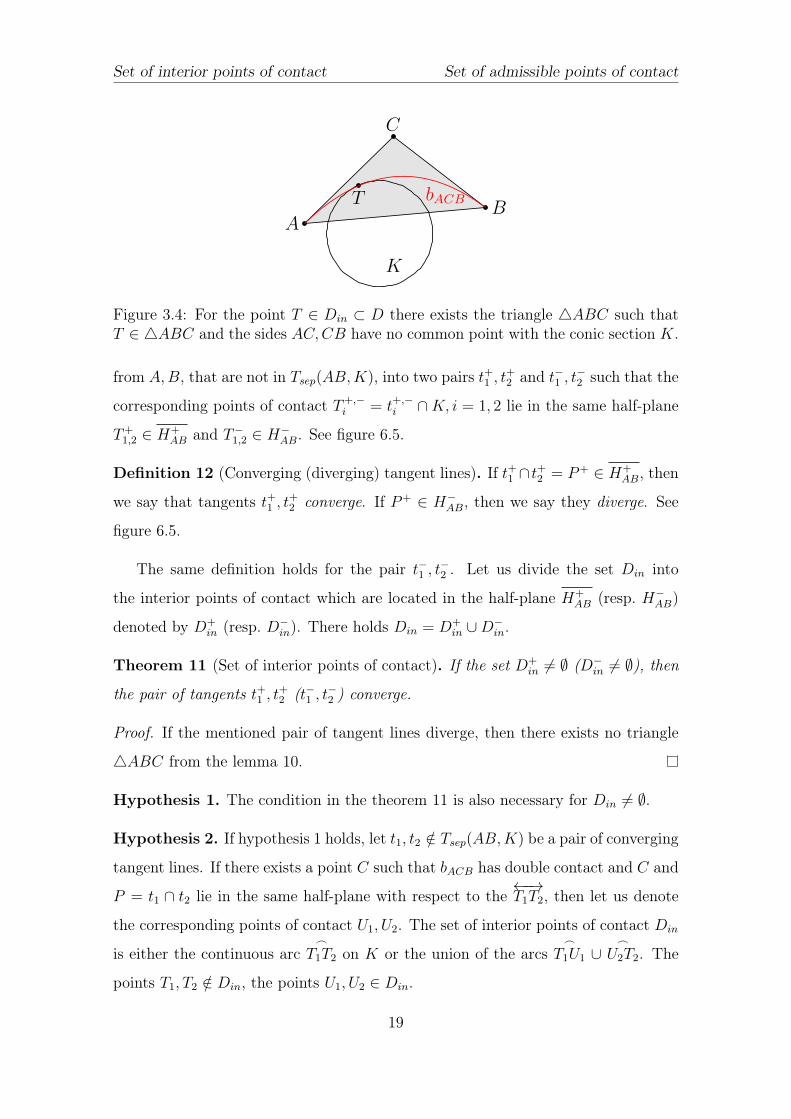
Lemma 10. If T ∈ Din ⊂ D is an interior point of contact of the Bézier curve b(t)
and the conic section K, then there exists the triangle 4ABC such that T ∈ 4ABC
and the sides AC,CB have no common point with the conic section K, see fig. 3.4.
Proof. Let the Bézier curve bACB be determined by the end points A,B and the
tangent line t at the point T ∈ K ∩ bACB. Then, the triangle 4ABC determined by
the control points of the Bézier curve satisfies the requirements of the lemma. The
point T ∈ 4ABC because the Bézier curve is completely contained in the convex
hull of its control points. The sides AC,CB have no common point with the conic
section K because they are separated from K by the curve bACB.
The line←→AB divides the plane ρ into two half-planes, the open half-plane H−AB,
and the closed half-plane H+AB such that
←→AB ⊂ H+
AB. Let us divide tangent lines
18
Set of interior points of contact Set of admissible points of contact
AB
C
T
K
bACB
Figure 3.4: For the point T ∈ Din ⊂ D there exists the triangle 4ABC such thatT ∈ 4ABC and the sides AC,CB have no common point with the conic section K.
from A,B, that are not in Tsep(AB,K), into two pairs t+1 , t+2 and t−1 , t
−2 such that the
corresponding points of contact T+,−i = t+,−i ∩K, i = 1, 2 lie in the same half-plane
T+1,2 ∈ H+
AB and T−1,2 ∈ H−AB. See figure 6.5.
Definition 12 (Converging (diverging) tangent lines). If t+1 ∩ t+2 = P+ ∈ H+AB, then
we say that tangents t+1 , t+2 converge. If P+ ∈ H−AB, then we say they diverge. See
figure 6.5.
The same definition holds for the pair t−1 , t−2 . Let us divide the set Din into
the interior points of contact which are located in the half-plane H+AB (resp. H−AB)
denoted by D+in (resp. D−in). There holds Din = D+
in ∪D−in.
Theorem 11 (Set of interior points of contact). If the set D+in 6= ∅ (D−in 6= ∅), then
the pair of tangents t+1 , t+2 (t−1 , t
−2 ) converge.
Proof. If the mentioned pair of tangent lines diverge, then there exists no triangle
4ABC from the lemma 10.
Hypothesis 1. The condition in the theorem 11 is also necessary for Din 6= ∅.
Hypothesis 2. If hypothesis 1 holds, let t1, t2 /∈ Tsep(AB,K) be a pair of converging
tangent lines. If there exists a point C such that bACB has double contact and C and
P = t1 ∩ t2 lie in the same half-plane with respect to the←−→T1T2, then let us denote
the corresponding points of contact U1, U2. The set of interior points of contact Din
is either the continuous arc_
T1T2 on K or the union of the arcs_
T1U1 ∪_
U2T2. The
points T1, T2 /∈ Din, the points U1, U2 ∈ Din.
19
Set of points of contact Set of admissible points of contact
Note 6. IfDin contains a set {_
T1U1 ∪_
U2T2}, we will call the union of two continuous
arcs_
T1U1 and_
U2T2 by sharp arc (see fig. 6.4). Later, we will see that the union of
these two arcs will have the same properties as a continuous arc of interior touches_
T1T2. So this sharp is just apparent and this union has structural properties for our
use as a continuous arc.
3.3 Set of points of contact
As we said, the set of all points of contact D = Dext ∪Din. The following theorem
describes the set D for different regular types of conic section K.
Theorem 12 (Set of points of contact).
(a) Let K be an ellipse. Then, the set of the points of contact D is either one arc
of the exterior points of contact or one arc of exterior and one arc of interior
points of contact or one or two arcs of interior points of contact.
(b) Let K be a parabola. Then, the set of the points of contact D is either one arc
of the exterior points of contact or one arc of interior points of contact.
(c) Let K be a hyperbola. Then, the set of the points of contact D is either two arcs
of the exterior points of contact or one arc of exterior and one arc of interior
points of contact.
The arcs of the interior points of contact may be sharp. The set of exterior points
of contact may contains only one point T0, when segment AB ∩K = {T0}.
Proof. a) (Ellipse) Let AB ∩K = ∅. Then among all tangents from A and B to K,
there are two in the set Tsep(AB,K). They determine one arc Dext. The other two
tangents are not in the set Tsep(AB,K). If they converge, then there is also one arc
Din. If they diverge, Din = ∅. If AB ∩K = {T0}, the only difference is that from
separating pair of tangent lines become one line←→AB and Dext = {T0}.
Let AB ∩ K = {X1, X2}. Then, we consider two pairs of tangent lines t+1 , t+2
and t−1 , t−2 . One pair, without loss of generality the pair t+1 , t
+2 , always converge
20
Set of points of contact Set of admissible points of contact
so D+in 6= ∅. The pair t−1 , t
−2 may converge or diverge, so we can obtain D as one or
two arcs of Din.
b) (Parabola) Let AB ∩K = ∅. Then among all tangents from A and B to K,
there are two in the set Tsep(AB,K). They determine one arc Dext. The other two
tangents are not in the set Tsep(AB,K), but they always diverge so Din = ∅. Hence,
we obtain D as one arc Dext. If AB ∩K = {T0}, then D = Dext = {T0}.
Let AB ∩K = {X1, X2}. Without loss of generality, the pair t+1 , t+2 always converge
so D+in 6= ∅ and the pair t−1 , t
−2 always diverge so D−in = ∅. Hence, we obtain D as
one arc Din.
c) (Hyperbola) Each component K1, K2 of a hyperbola K separately behaves
similarly to the parabola case. There are two cases of configuration AB and K1, K2.
The first, AB ∩K1 = ∅ and also AB ∩K2 = ∅. Then, we obtain D as two arcs of
Dext. If AB ∩K1 = {T0}, the only difference is that D1ext = {T0} (similarly for K2
if AB ∩K2 = {T0}).
The second case, AB ∩K1 = ∅ and AB ∩K2 = {X1, X2}. Then we obtain D as one
arc of Dext ⊂ K1 and one arc of Din ⊂ K2. There are no other configurations.
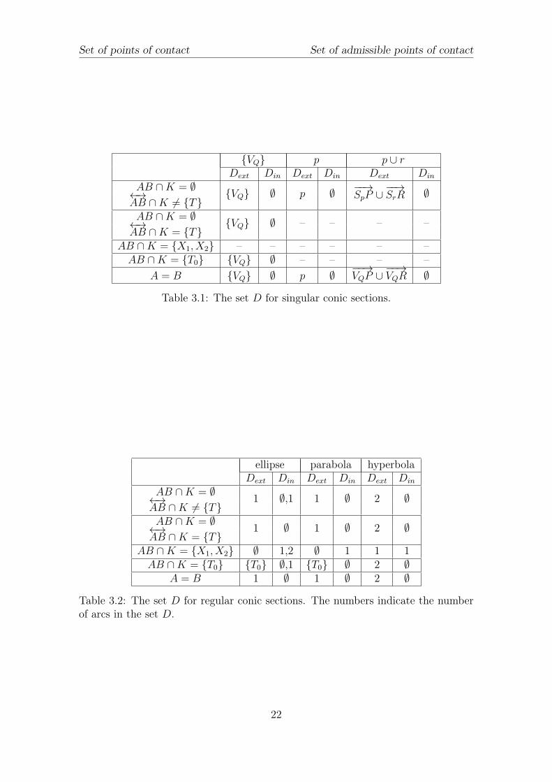
In the tables 3.1 and 3.2, we see the structure of the set D looks like for various
types of conic sections. The numbers in the table 3.2 represent the number of arcs
in the set D. The generic cases for regular and singular conic sections are illustrated
in chapter 6.
21
Set of points of contact Set of admissible points of contact
{VQ} p p ∪ rDext Din Dext Din Dext Din
AB ∩K = ∅ {VQ} ∅ p ∅ −−→SpP ∪
−−→SrR ∅←→
AB ∩K 6= {T}AB ∩K = ∅ {VQ} ∅ – – – –←→AB ∩K = {T}
AB ∩K = {X1, X2} – – – – – –AB ∩K = {T0} {VQ} ∅ – – – –
A = B {VQ} ∅ p ∅−−→VQP ∪
−−→VQR ∅
Table 3.1: The set D for singular conic sections.
ellipse parabola hyperbolaDext Din Dext Din Dext Din
AB ∩K = ∅ 1 ∅,1 1 ∅ 2 ∅←→AB ∩K 6= {T}AB ∩K = ∅ 1 ∅ 1 ∅ 2 ∅←→AB ∩K = {T}
AB ∩K = {X1, X2} ∅ 1,2 ∅ 1 1 1AB ∩K = {T0} {T0} ∅,1 {T0} ∅ 2 ∅
A = B 1 ∅ 1 ∅ 2 ∅
Table 3.2: The set D for regular conic sections. The numbers indicate the numberof arcs in the set D.
22
Chapter 4
Boundary map
For the given points A,B, X ∈ D \De ⊆ K and the tangent line t at X to K, the
Bézier curve bACB touching the conic section K is clearly identified. In order to find
the middle control vertex C, we use the following map σ. This map is very similar
to the map τ from the chapter 1, only the direction vector of the line t is expressed
by the coefficients of the conic section K.
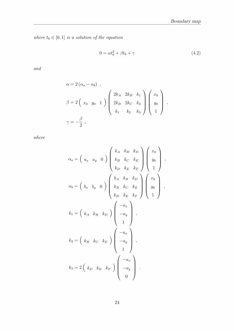
Definition 13 (Boundary map). Let D be the set of points of contact for the given
space-like points A,B and K. The map σ : D \De → R21 is called boundary map if
for every X ∈ D \De holds σ(X) = C, for C from the definition 8, see the fig. 4.1.
Note 7. It is not possible to define the map σ on the points in De. If T ∈ De ⊂ K
then points A,B, T are collinear on the tangent line t to K. And there is an infinite
number of points C such that Bézier curve bACB touches K in T . All suitable C
form a half-line, therefore we are interested in the end point of the half-line, the
point CS.
Theorem 13. Let the conic section K 6= {VQ} and X = [x0, y0] ∈ D \ De. Then
the corresponding boundary map σ : D \De → R21 has the form
σ(X) =b(t0)−B2
0(t0)A−B22(t0)B
B21(t0)
, (4.1)
23
Boundary map
where t0 ∈ [0, 1] is a solution of the equation
0 = αt20 + βt0 + γ (4.2)
and
α = 2 (αa − αb) ,
β = 2(x0 y0 1
)2kA 2kB k1
2kB 2kC k2
k1 k2 k3
x0
y0
1
,
γ = −β2,
where
αa =(ax ay 0
)kA kB kD
kB kC kE
kD kE kF
x0
y0
1
,
αb =(bx by 0
)kA kB kD
kB kC kE
kD kE kF
x0
y0
1
,
k1 =(kA kB kD
)−ax−ay
1
,
k2 =(kB kC kE
)−ax−ay
1
,
k3 = 2(kD kE kF
)−ax−ay
0
.
24
Boundary map
A
BK
C
∂V
D
T
Figure 4.1: The boundary map σ, see that σ(T ) = C.
Proof. Since we consider only real points C ∈ ρ, let K = {[x, y] ∈ R2 : kAx2 +
2kBxy + kCy2 + 2kDx + 2kEy + kF = 0}. Because of the point of the contact
X ∈ bACB(t), there exists t0 ∈ [0, 1] such that X = bACB(t0) = B20(t0)A+B2
1(t0)C+
B22(t0)B. The point X ∈ K is light-like so X /∈ {A,B} and t0 /∈ {0, 1}. Because
X = [x0, y0] ∈ D \De then holds⟨∇f(x0, y0),
ddtbACB(t0)
⟩= 0. From this quadratic
equation we obtain two roots t00, t10, but only one is in (0, 1). If both t00, t10 ∈ (0, 1)
and t00 6= t10 then X ∈ De. Let t00 ∈ (0, 1). Then we substitute t0 = t00 into the Bézier
curve equation and obtain relevant point C from the definition 8 for the point of
the contact X. Hence, C = σ(X).
Theorem 14. For each X ∈ D \De there exists exactly one point C such that the
Bézier curve bACB(t) ∩K = {X}.
Proof. Let t ∈ TK touches the conic section in the point X ∈ K. We know, that the
Bézier curve bACB has the points A,B as the end points, it contains the point X and
it has the tangent line t at X. Hence, using the theorem 1, the quadratic bACB is
uniquely determined up to the case A,B,X ∈ t are collinear. But then X ∈ De.
25
Chapter 5
Area of admissible solutions
Lemma 15. The boundary map σ is injective for the set D \De up to the points Ui.
Proof. Let X1, X2 ∈ D\{De∪{Ui}} ⊂ K, X1 6= X2 and σ(X1) = σ(X2) = C. Then,
there exists a double contact Bézier curve bACB such that X1, X2 are the points of
contact. Then {X1, X2} = {U1, U2}, which is a contradiction.
Note 8. Let the sharp arc {_
T1U1 ∪_
U2T2} ⊂ Din. The image σ(_
T1U1 −{T1}) is a
connected curve l1, because the boundary map σ is a continuous map. Also, the
image σ(_
U2T2 −{T2}) is a connected curve l2. There exists a point Cu such that the
intersection bACuB ∩K = {U1, U2}, hence, Cu ∈ l1 and Cu ∈ l2. Simultaneously, the
points U1, U2 are the end points of the continuous arcs_
T1U1 and_
U2T2. Hence, the
image of the sharp arc under the boundary map σ is the connected curve l = l1 ∪ l2(see the figure 6.4).
Now, we can find the corresponding point C for the points of contact from the
set D \De. The question is, how can we find the point C corresponding to a given
point of contact T ∈ De ⊂ D.
Lemma 16. Let the points A,B and T ∈ De ⊂ K be collinear.
(a) Let AB ∩K = {T}. The Bézier curve bACB ∩K = {T} if and only if C ∈←→AB.
(b) Let AB ∩ K = ∅. The Bézier curve bACB ∩ K = {T} if and only if C ∈−−→CSX ⊂
←→AB, where A,B /∈
−−→CSX and CS is such that the derivative bACSB(t0) = 0
for T = bACSB(t0). For the special case A = B, then the point CS = A+ 2(T − A).
26
Area of admissible solutions
Proof. Because A,B, T are collinear, the point C ∈←→AB. In the case (b), if C
belongs to the opposite half-line to−−→CSX, the Bézier curve and conic section have
no common points.
Note 9. In the equation (4.1) of the boundary map σ, the inequality B21(t0) > 0
holds for t0 ∈ (0, 1), so the map σ is continuous. The σ maps the connected set
Dext \De onto one connected curve l. If the point T ∈ De 6= ∅, then limX→T σ(X) =
CS and the union l ∪−−→CSX is a connected curve.
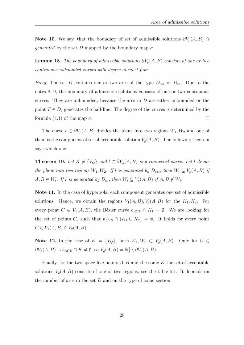
Theorem 17 (Boundary of the set Vρ(A,B)). The set of all feasible points C such
that bACB ∩K ⊂ D, is the boundary of the set of admissible solutions Vρ(A,B). We
denote it ∂Vρ(A,B).
Proof. The point C belongs to the boundary of the set Vρ(A,B), if each neighbour-
hood N of the point C contains both the point C1 ∈ Vρ(A,B) and C2 /∈ Vρ(A,B).
So, we prove the existence of points C1, C2 ∈ N such that bAC1B ∩ K = ∅ and
bAC2B ∩K = {X1, X2} with transversed intersection (see fig. 5.1).
Let A,B, u as in the theorem 1 be fixed. Since B21(t0) > 0 for t0 ∈ (0, 1), the
map τ , which assign to each T the corresponding point C, is continuous. It means,
for each neighbourhood N of the point C exists the neighbourhood M of the point
T such that τ(M) ⊂ N .
Let C be such that bACB ∩ K ⊂ D and T ∈ bACB ∩ K. Let the line t with
the direction vector u is the tangent line to K in T . From above, for arbitrary
neighbourhood N of the point C exists the neighbourhood M of the point T such
that τ(M) ⊂ N . Let T1 = T + k∇f(T ) and T2 = T − k∇f(T ), where k > 0 is
such that T1, T2 ∈ M and they satisfies the requirements of the theorem 1. Let
the lines t1, t2 be parallel to the line t (i.e. the vector u is their direction vector)
and T1 ∈ t1, T2 ∈ t2. Then the points C1 = τ(A,B, T1, u) and C2 = τ(A,B, T2, u)
are C1, C2 ∈ N . We obtain the Bézier curves bAC1B, bAC2B. Since each tangent line
t1, t2 defines the supporting half-plane to the convex quadratic Bézier curve and the
points A,B are space-like, it holds bAC1B ∩K = ∅ and bAC2B ∩K = {X1, X2} with
transversed intersection.
27
Area of admissible solutions
Note 10. We say, that the boundary of set of admissible solutions ∂Vρ(A,B) is
generated by the set D mapped by the boundary map σ.
Lemma 18. The boundary of admissible solutions ∂Vρ(A,B) consists of one or two
continuous unbounded curves with degree at most four.
Proof. The set D contains one or two arcs of the type Dext or Din. Due to the
notes 8, 9, the boundary of admissible solutions consists of one or two continuous
curves. They are unbounded, because the arcs in D are either unbounded or the
point T ∈ De generates the half-line. The degree of the curves is determined by the
formula (4.1) of the map σ.
The curve l ⊂ ∂Vρ(A,B) divides the plane into two regions W1,W2 and one of
them is the component of set of acceptable solution Vρ(A,B). The following theorem
says which one.
Theorem 19. Let K 6= {VQ} and l ⊂ ∂Vρ(A,B) is a connected curve. Let l divide
the plane into two regions W1,W2. If l is generated by Dext, then Wi ⊆ Vρ(A,B) if
A,B ∈ Wi. If l is generated by Din, then Wi ⊆ Vρ(A,B) if A,B 6∈ Wi.
Note 11. In the case of hyperbola, each component generates one set of admissible
solutions. Hence, we obtain the regions V1(A,B), V2(A,B) for the K1, K2. For
every point C ∈ V1(A,B), the Bézier curve bACB ∩ K1 = ∅. We are looking for
the set of points C, such that bACB ∩ (K1 ∪ K2) = ∅. It holds for every point
C ∈ V1(A,B) ∩ V2(A,B).
Note 12. In the case of K = {VQ}, both W1,W2 ⊂ Vρ(A,B). Only for C ∈
∂Vρ(A,B) is bACB ∩K 6= ∅, so Vρ(A,B) = R21 \ ∂Vρ(A,B).
Finally, for the two space-like points A,B and the conic K the set of acceptable
solutions Vρ(A,B) consists of one or two regions, see the table 5.1. It depends on
the number of arcs in the set D and on the type of conic section.
28
Area of admissible solutions
M
τ (M)
N
K
C
A
B
∂V
D
C1
C2TT1
T2
Figure 5.1: Let C be such that bACB ∩ K ⊂ D and T ∈ bACB ∩ K. For arbitraryneighbourhood N of the point C, there exists a neighbourhood M of the point Tsuch that for T1, T2 ∈M the corresponding C1 = τ(T1), C2 = τ(T2) ∈ N . Moreover,bAC1B ∩ K = ∅ and bAC2B ∩ K = {X1, X2} with transversed intersection. Hence,C ∈ ∂Vρ(A,B).
{VQ} p p ∪ r ellipse parabola hyperbolaAB ∩K = ∅ 2 1 1 1,2 1 1←→AB ∩K 6= {T}AB ∩K = ∅ 1 – – 1 1 1←→AB ∩K = {T}
AB ∩K = {X1, X2} – – – 1,2 1 1AB ∩K = {T0} 2 – – 1,2 1 1
A = B 1 1 1 1 1 1
Table 5.1: The number of regions in the set of acceptable solutions Vρ(A,B).
29
Chapter 6
Examples
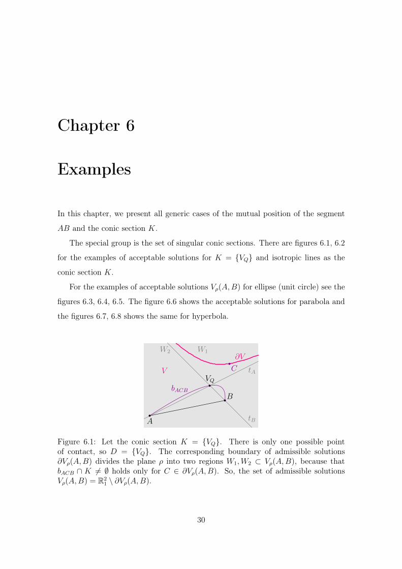
In this chapter, we present all generic cases of the mutual position of the segment
AB and the conic section K.
The special group is the set of singular conic sections. There are figures 6.1, 6.2
for the examples of acceptable solutions for K = {VQ} and isotropic lines as the
conic section K.
For the examples of acceptable solutions Vρ(A,B) for ellipse (unit circle) see the
figures 6.3, 6.4, 6.5. The figure 6.6 shows the acceptable solutions for parabola and
the figures 6.7, 6.8 shows the same for hyperbola.
tA
tBA
B
∂VW1W2
VQ
V C
bACB
Figure 6.1: Let the conic section K = {VQ}. There is only one possible pointof contact, so D = {VQ}. The corresponding boundary of admissible solutions∂Vρ(A,B) divides the plane ρ into two regions W1,W2 ⊂ Vρ(A,B), because thatbACB ∩ K 6= ∅ holds only for C ∈ ∂Vρ(A,B). So, the set of admissible solutionsVρ(A,B) = R2
1 \ ∂Vρ(A,B).
30
Examples
A
BK
D
∂V
V
C
bACB
T
A
BK
D ∂V
VP
R
Cu
Sr
Sp
(a) (b)
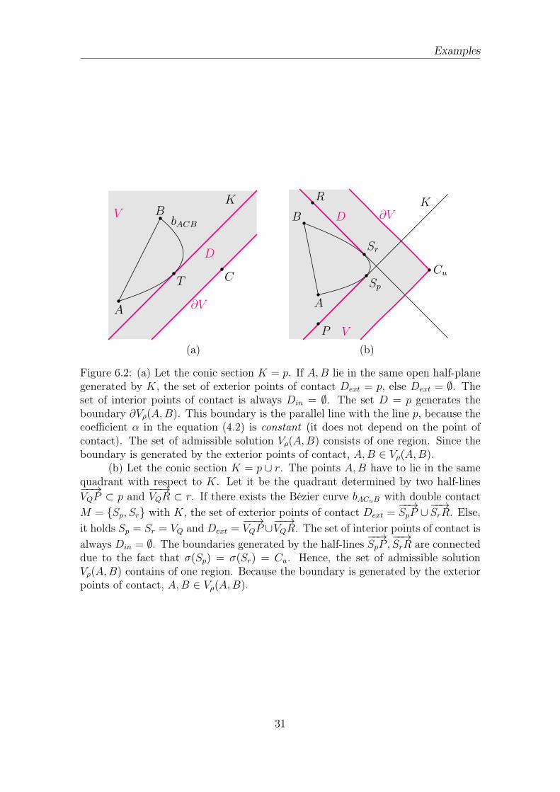
Figure 6.2: (a) Let the conic section K = p. If A,B lie in the same open half-planegenerated by K, the set of exterior points of contact Dext = p, else Dext = ∅. Theset of interior points of contact is always Din = ∅. The set D = p generates theboundary ∂Vρ(A,B). This boundary is the parallel line with the line p, because thecoefficient α in the equation (4.2) is constant (it does not depend on the point ofcontact). The set of admissible solution Vρ(A,B) consists of one region. Since theboundary is generated by the exterior points of contact, A,B ∈ Vρ(A,B).
(b) Let the conic section K = p ∪ r. The points A,B have to lie in the samequadrant with respect to K. Let it be the quadrant determined by two half-lines−−→VQP ⊂ p and
−−→VQR ⊂ r. If there exists the Bézier curve bACuB with double contact
M = {Sp, Sr} with K, the set of exterior points of contact Dext =−−→SpP ∪
−−→SrR. Else,
it holds Sp = Sr = VQ and Dext =−−→VQP ∪
−−→VQR. The set of interior points of contact is
always Din = ∅. The boundaries generated by the half-lines−−→SpP ,
−−→SrR are connected
due to the fact that σ(Sp) = σ(Sr) = Cu. Hence, the set of admissible solutionVρ(A,B) contains of one region. Because the boundary is generated by the exteriorpoints of contact, A,B ∈ Vρ(A,B).
31
Examples
A
B K
T1B
T2B
T1A
T2A
P
D
∂V
V
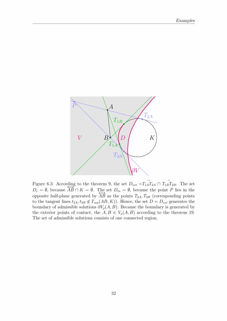
Figure 6.3: According to the theorem 9, the set Dext =_
T1AT2A ∩_
T1BT2B. The setDe = ∅, because
←→AB ∩ K = ∅. The set Din = ∅, because the point P lies in the
opposite half-plane generated by←→AB as the points T2A, T2B (corresponding points
to the tangent lines t2A, t2B /∈ Tsep(AB,K)). Hence, the set D = Dext generates theboundary of admissible solutions ∂Vρ(A,B). Because the boundary is generated bythe exterior points of contact, the A,B ∈ Vρ(A,B) according to the theorem 19.The set of admissible solutions consists of one connected region.
32
Examples
A
B
T1B
T2BT1A
T2A
U1
U2
P
K
bACuB
D
l1 l2
W 11 W 2
1
W 12
W 22
VV
Cu
Figure 6.4: The set Dext =_
T1AT2A ∩_
T1BT2B. The set Din 6= ∅, because the pointP lies in the same half-plane generated by
←→AB as the points T2A, T2B. The set Din
is the sharp arc_
T2AU1 ∪_
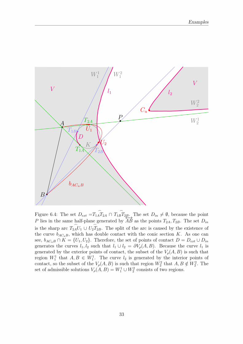
U2T2B. The split of the arc is caused by the existence ofthe curve bACuB, which has double contact with the conic section K. As one cansee, bACuB ∩K = {U1, U2}. Therefore, the set of points of contact D = Dext ∪Din
generates the curves l1, l2 such that l1 ∪ l2 = ∂Vρ(A,B). Because the curve l1 isgenerated by the exterior points of contact, the subset of the Vρ(A,B) is such thatregion W 1
1 that A,B ∈ W 11 . The curve l2 is generated by the interior points of
contact, so the subset of the Vρ(A,B) is such that region W 22 that A,B /∈ W 2
2 . Theset of admissible solutions Vρ(A,B) = W 1
1 ∪W 22 consists of two regions.
33
Examples
A
B
T+2
T−2
T+1
T−1
H+AB H−
AB
P+P− KD
∂V
V
A
B
H+AB H−
AB
P+ P−
K
D
l1 l2
V V
T+2 T−
2
T+1 T−
1
(a) (b)
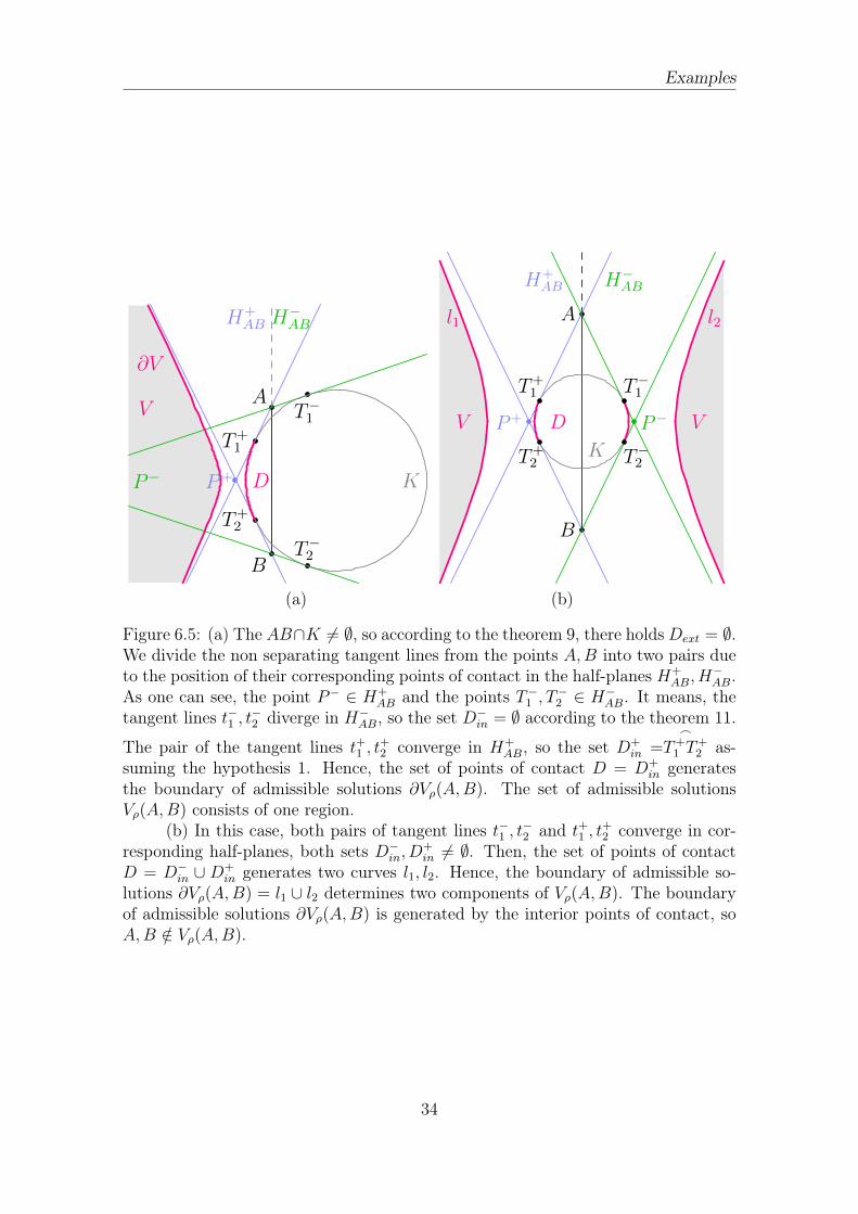
Figure 6.5: (a) The AB∩K 6= ∅, so according to the theorem 9, there holdsDext = ∅.We divide the non separating tangent lines from the points A,B into two pairs dueto the position of their corresponding points of contact in the half-planes H+
AB, H−AB.
As one can see, the point P− ∈ H+AB and the points T−1 , T
−2 ∈ H−AB. It means, the
tangent lines t−1 , t−2 diverge in H−AB, so the set D−in = ∅ according to the theorem 11.
The pair of the tangent lines t+1 , t+2 converge in H+
AB, so the set D+in =
_
T+1 T
+2 as-
suming the hypothesis 1. Hence, the set of points of contact D = D+in generates
the boundary of admissible solutions ∂Vρ(A,B). The set of admissible solutionsVρ(A,B) consists of one region.
(b) In this case, both pairs of tangent lines t−1 , t−2 and t+1 , t
+2 converge in cor-
responding half-planes, both sets D−in, D+in 6= ∅. Then, the set of points of contact
D = D−in ∪ D+in generates two curves l1, l2. Hence, the boundary of admissible so-
lutions ∂Vρ(A,B) = l1 ∪ l2 determines two components of Vρ(A,B). The boundaryof admissible solutions ∂Vρ(A,B) is generated by the interior points of contact, soA,B /∈ Vρ(A,B).
34
Examples
A
B
T2A
P
K
D
∂V
V
T1A
T1B
T2B
A B
t+1t+2
t−1 t−2
P+
H+AB
K
D
∂V
V
T+1 T+
2
(a) (b)
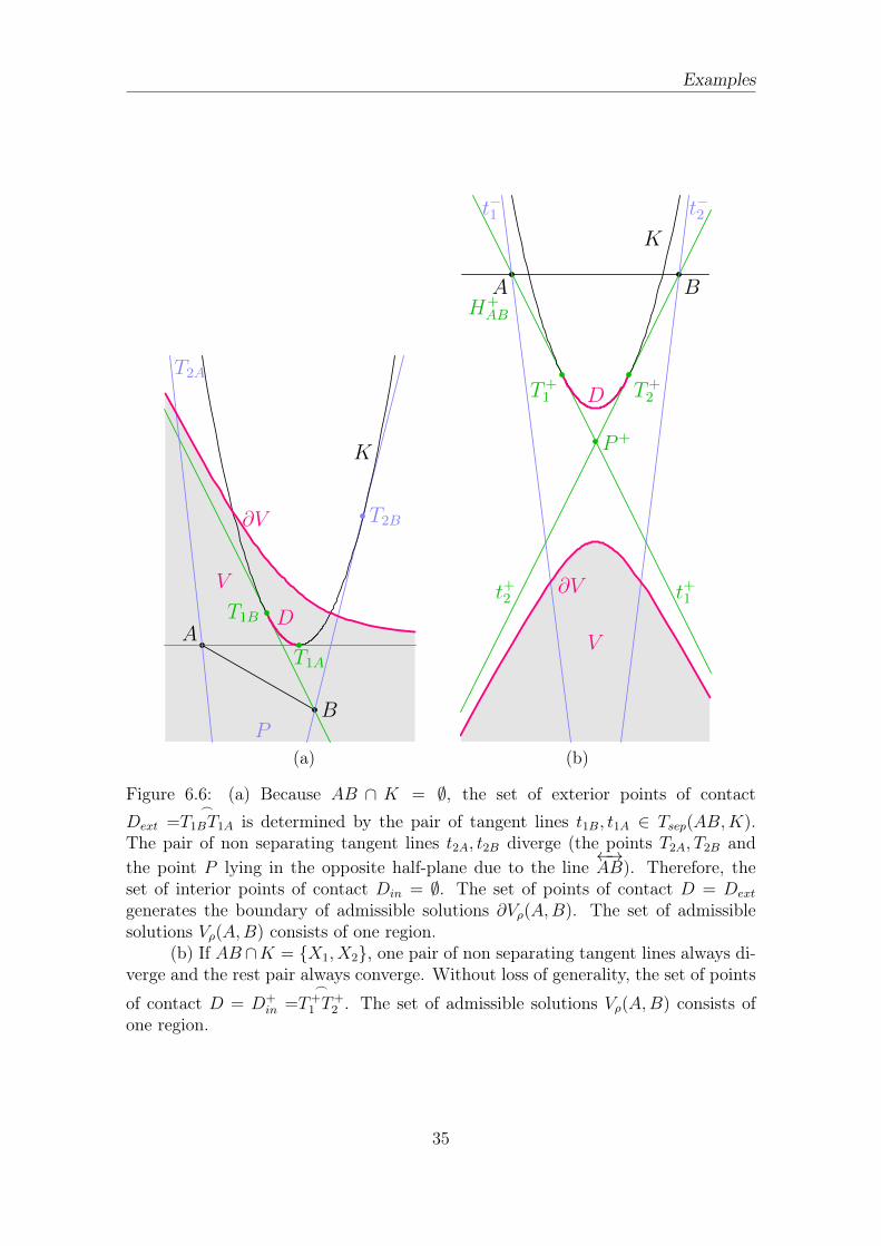
Figure 6.6: (a) Because AB ∩ K = ∅, the set of exterior points of contactDext =
_
T1BT1A is determined by the pair of tangent lines t1B, t1A ∈ Tsep(AB,K).The pair of non separating tangent lines t2A, t2B diverge (the points T2A, T2B andthe point P lying in the opposite half-plane due to the line
←→AB). Therefore, the
set of interior points of contact Din = ∅. The set of points of contact D = Dext
generates the boundary of admissible solutions ∂Vρ(A,B). The set of admissiblesolutions Vρ(A,B) consists of one region.
(b) If AB ∩K = {X1, X2}, one pair of non separating tangent lines always di-verge and the rest pair always converge. Without loss of generality, the set of points
of contact D = D+in =
_
T+1 T
+2 . The set of admissible solutions Vρ(A,B) consists of
one region.
35
Examples
K1K2
a1
a2
a∞1
A
B
T1BT2B
T1A
T2A
D1D2
l1
l2
W 11 W 1
2
W 21 W 2
2
V
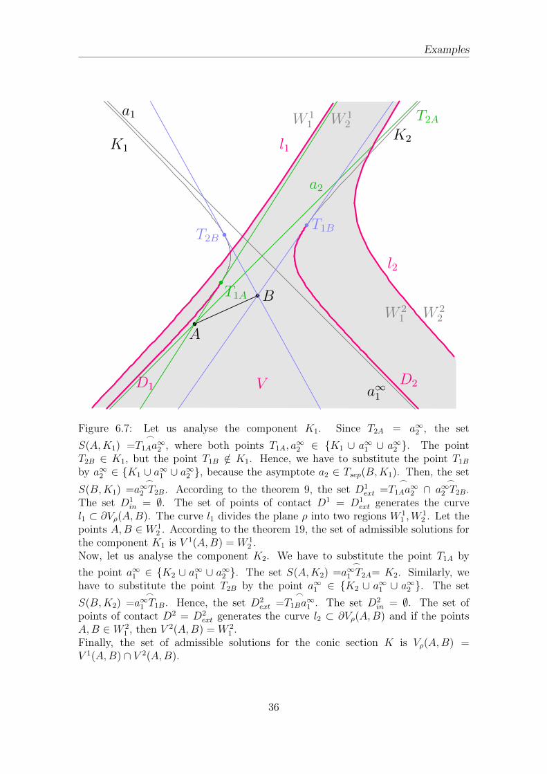
Figure 6.7: Let us analyse the component K1. Since T2A = a∞2 , the setS(A,K1) =
_
T1Aa∞2 , where both points T1A, a∞2 ∈ {K1 ∪ a∞1 ∪ a∞2 }. The point
T2B ∈ K1, but the point T1B /∈ K1. Hence, we have to substitute the point T1Bby a∞2 ∈ {K1 ∪ a∞1 ∪ a∞2 }, because the asymptote a2 ∈ Tsep(B,K1). Then, the set
S(B,K1) =_
a∞2 T2B. According to the theorem 9, the set D1ext =
_
T1Aa∞2 ∩
_
a∞2 T2B.The set D1
in = ∅. The set of points of contact D1 = D1ext generates the curve
l1 ⊂ ∂Vρ(A,B). The curve l1 divides the plane ρ into two regions W 11 ,W
12 . Let the
points A,B ∈ W 12 . According to the theorem 19, the set of admissible solutions for
the component K1 is V 1(A,B) = W 12 .
Now, let us analyse the component K2. We have to substitute the point T1A bythe point a∞1 ∈ {K2 ∪ a∞1 ∪ a∞2 }. The set S(A,K2) =
_
a∞1 T2A= K2. Similarly, wehave to substitute the point T2B by the point a∞1 ∈ {K2 ∪ a∞1 ∪ a∞2 }. The setS(B,K2) =
_
a∞1 T1B. Hence, the set D2ext =
_
T1Ba∞1 . The set D2
in = ∅. The set ofpoints of contact D2 = D2
ext generates the curve l2 ⊂ ∂Vρ(A,B) and if the pointsA,B ∈ W 2
1 , then V 2(A,B) = W 21 .
Finally, the set of admissible solutions for the conic section K is Vρ(A,B) =V 1(A,B) ∩ V 2(A,B).
36
Examples
K1 K2
a1 a2
A
B
T1B
T2B
T1A
T2A
D1 D2
l1
l2
V
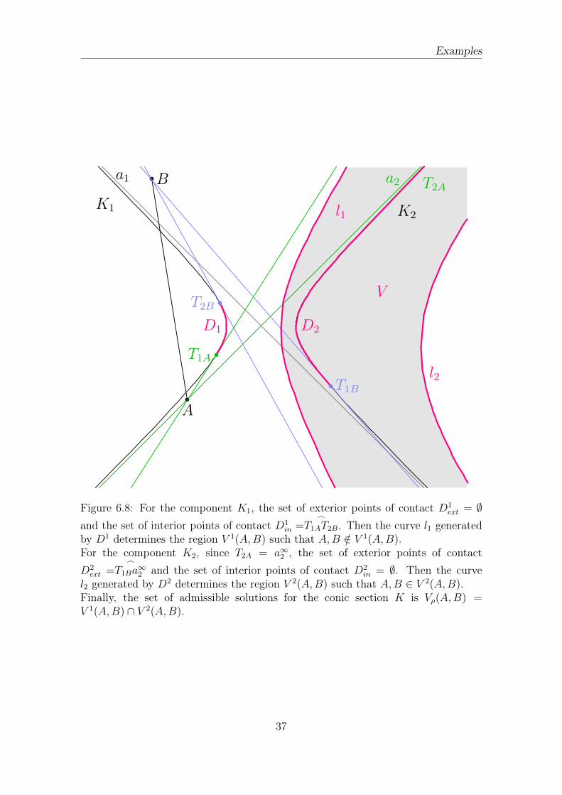
Figure 6.8: For the component K1, the set of exterior points of contact D1ext = ∅
and the set of interior points of contact D1in =
_
T1AT2B. Then the curve l1 generatedby D1 determines the region V 1(A,B) such that A,B /∈ V 1(A,B).For the component K2, since T2A = a∞2 , the set of exterior points of contactD2ext =
_
T1Ba∞2 and the set of interior points of contact D2
in = ∅. Then the curvel2 generated by D2 determines the region V 2(A,B) such that A,B ∈ V 2(A,B).Finally, the set of admissible solutions for the conic section K is Vρ(A,B) =V 1(A,B) ∩ V 2(A,B).
37
Chapter 7
Conclusion
For the given points A,B in three dimensional Minkowski space, we described the
area V (A,B) of all such points C that the quadratic Bézier curve with control points
A,C,B is space-like.
For this purpose, we define the necessary conditions for the end points A,B of
the Bézier curve. Then, we fixed the points A,B and we looked for the admissible
points C. We solved the problem for each type of conic section K, which the plane
ρ containing the points A,B cuts in the light cone Q.
The area Vρ(A,B) containing the admissible points C ∈ ρ is described via method
of contact point. We proved, that the boundary of this area ∂Vρ(A,B) is determined
by such points C that bACB touches to the conic section K. Hence, we found the set
of admissible points of contact D for the given points A,B as union of exterior and
interior points of contact. Then, we showed how the set D determines boundary
∂Vρ(A,B) using the boundary map σ.
We have illustrated this study with typical examples, which show the area Vρ(A,B)
for each type of conic section K.
When the hypothesis 1, 2 are solved, then the case of quadratic space-like curves
will be completed. We have indications leading to the proves, they still must be
elaborated.
38
Project of Dissertation
In this chapter, we present the plan of our future work. We want to focus on con-
clusion of space-like conditions for quadratic curves. In the rest of our study, we
will look for the space-like condition of the Bézier curves of higher degree in three
dimensional Minkowski space. We start to study a conditions for cubic curves, using
the knowledge and methods from quadratic case as much as possible. Additional
methods are to be applied too.
Future research
We would like to proof the hypothesis 1, 2 on the set of interior points of contact.
Then, the space-like conditions for the control points of the quadratic curve will be
entirely completed.
In order to prove the hypothesis 1, we use that if the pair of tangent lines t+1 , t+2
converge in the half-plane H+AB, then the lines v1, v2 from the points A,B, which are
orthogonal to the segment AB, have no common points with K in the half-plane
H+AB. Let the lines v1, v2 determine the point at infinity v∞. In order to D+
in 6= ∅,
there have to exists the Bézier curve b(t) ⊂ H+AB such that b(t) ∩K = ∅. We use as
"the limit case" that the Bézier curve bAv∞B ∩K = ∅.
Regarding the hypothesis 2, let the quadratic Bézier curve bACB(t) be a part of the
parabolic arc pC . We denote the curvature of the curve pC at the point X ∈ pC by
κ (pC , X). Let the point PC ∈ bACB ⊂ pC is such that for arbitrary X ∈ bACB ⊂ pC
holds κ (pC , PC) ≥ κ (pC , X). Let the sharp arc {_
T1U1 ∪_
U2T2} ∈ Din generate
the connected curve l ∈ ∂Vρ(A,B). For verification of the hypothesis 2, we use
39
Project of Dissertation
the following hypothesis. The point Cu ∈ l is such that for arbitrary C ∈ l holds
κ (pCu , PCu) ≤ κ (pC , PC).
After the proof of both hypothesis, the set of admissible solutions will be found for
the each type of conic section in the plane ρ.
Until now, we illustrate the situation only in the plane. Hence, we would like to
make a 3D visualisation of the situation. We will fix the points A,B and we will con-
sider a several positions of the plane ρ. We present a model of set of all admissible
solutions to the problem describing its surface boundary. We detect its singularities.
The analytic expression of the boundary of admissible solutions in the plane ρ
is another interesting question. In order to find it, we express all definitions and
propositions using in this work by analytical equations and inequalities. Also, we
suppose that the parameter t for the points of contact changes continuously. We
look for the interval J ⊂ [0, 1] of the parameter t, and the expression of the bound-
ary from the equation (4.1) of the boundary map σ.
This generates the question, what kind of the object is the boundary in 3D? If we
know the analytic expression of the boundary in the plane, we parametrize it to
find the analytic expression of the boundary of the "spatial set of admissible solu-
tions". Clearly, the same approach can be used in arbitrary dimension for the case
of quadratic Bézier curves.
While looking for the set of points of contact D ⊂ K, we use the term point
at infinity. Then, in the case of K as hyperbola or parabola, our illustrations are
missing the points of the contact in the infinity. Inspired by the books on projective
geometry [Far99] and [Bix06], we would like to construct a spherical model of the
projective plane in order to compare the number of regions in the set of acceptable
solutions Vρ(A,B) with the current results. We suppose, the classification of all
possible cases for regular conic sections unifies and simplifies.
40
Project of Dissertation
After the conclusion of the quadratic case, we proceed to find analogous con-
ditions for the control points of cubic Bézier curves. The situation becomes much
more complicated, because cubic curves are uniquely determined by four control
points. In the past, we used the fact that quadratic curve lies in the plane. Hence,
we will consider the planar cubics first. We fix the three control points and we will
try to find (in the plane ρ) the set of admissible solutions for the remaining con-
trol point. We look for analytic conditions, which are visualized (e.g. by Asymptote).
An interesting topic covers considering rational curves in Minkowski space. Quad-
ratic case will be searched from the projective geometry point of view. The general
conditions for higher degree curves will be difficult to grasp. Hence, we consider cer-
tain classes such as rational curves with positive weight, convex curves and others
to gain insight into the structure of space-like curves.
In the case of general cubic curve, we plan to use the fact that the derivative of
cubic curve is a quadratic function although it might not be space-like. With the
fact that the end control points have to be space-like, we will try to get necessary
conditions for the control points or its linear combinations. If these are sufficient
conditions too, we verify it experimentally at first and theoretically later. We have
a hypothesis, that if the derivative is space-like (definition 1) along the curve and
end point is space-like, then the whole curve is space-like (definition 2). This leads
to certain class of cubic space-like curves putting together the results gained so far.
We try to combine the curve results to surface case for tensor-product surfaces.
41
Bibliography
[Ber87a] M. Berger. Geometry I. Universitext. Springer-Verlang, 1987. Translated
from the French by M. Cole and S. Levy.
[Ber87b] M. Berger. Geometry II. Universitext. Springer-Verlang, 1987. Translated
from the French by M. Cole and S. Levy.
[Bix06] R. Bix. Conics and Cubics. Springer, 2nd edition, 2006. ISBN: 978-0387-
31802-8.
[Cha10] P. Chalmovianský. Pseudo-euclidean spaces and hyperbolic geometry. Pro-
ceedings of Symposium on Computer Geometry, 19:109–114, 2010.
[CP11] P. Chalmovianský and B. Pokorná. Quadratic space-like Bézier curves
in the three dimensional Minkowski space. Proceedings of Symposium on
Computer Geometry, 20:104–110, 2011.
[DFN91] B., A. Dubrovin, A., T. Fomenko, and S., P. Novikov. Modern Geometry
- Methods and Applications: Part I: The Geometry of Surfaces, Transfor-
mation Groups, and Fields. Springer, 2nd edition, 1991.
[Far99] G. Farin. NURBS from Projective Geometry to Practical Use. AK Peters,
Ltd., 2nd edition, 1999. ISBN 1-56881-084-9.
[Gal10] B. Gallusová. Bézierove krivky a ich vlastnosti v Minkowského priestore.
Zborník príspevkov, Študentská vedecká konferencia FMFI UK, 2010.
[Geo08] M. Georgiev, editor. Space-like Bézier Curves in the three-dimensional
Minkowski Space, volume 1067. AIP Conference Proceedings, 2008.
42
BIBLIOGRAPHY BIBLIOGRAPHY
[Geo09] M. Georgiev, editor. Constructions of spacelike Bézier Surfaces in the
three-dimensional Minkowski Space, volume 1184. AIP Conference Pro-
ceedings, 2009.
[KJ06] J. Kosinka and B. Jüttler. Cubic Helices in Minkowski space. Sitzungsber.
Österr. Akad. Wiss., Abt. II, 215:13–35, 2006.
[KL10] J. Kosinka and M. Lávička. On Rational Minkowski Pythagorean Hodo-
graph Curves. Computer Aided Geometric Design, 27:514–524, 2010.
[Küh06] W. Kühnel. Differential Geometry: Curves – Surfaces – Manifolds. Ameri-
can Mathematical Society, 2nd edition, 2006. Translated from the German
by B. Hunt.
[Kun05] E. Kunz. Introduction to Plane Algebraic Curves. Birkhäuser, 2005.
[Mon03] J. Monterde. The Plateau-Bézier problem. Mathematics of Surfaces X,
2768:262–273, 2003.
[Mon04] J. Monterde. Bézier surfaces of minimal area: the dirichlet approach.
Computer Aided Geometric Design, 21:117–136, 2004.
[Pok11] B. Pokorná. Quadratic Bézier curves in the three dimensional Minkowski
space. Rigorózna práca, 2011.
[PŠ02] M. Petrović-Torgašev and E. Šućurović. W-curves in Minkowski space-
time. Novi Sad Journal of Mathematics, 32:55–65, 2002.
[UMY11] H. Ugail, M. C. Márquez, and A. Yilmaz. On Bézier Surfaces in the
three dimensional Minkowski space. Computers and Mathematics with
Applications, 62, 2011.
[YT08] S. Yilmaz and M. Turgut. On the Differential Geometry of the Curves in
Minkowski Space-time I. International Journal of Contemporary Mathe-
matical Sciences, 3:1343 – 1349, 2008.
43
List of Tables
3.1 The set D for singular conic sections . . . . . . . . . . . . . . . . . . 22
3.2 The set D for regular conic sections . . . . . . . . . . . . . . . . . . . 22
5.1 The number of regions in the set of acceptable solutions Vρ(A,B) . . 29
44
List of Figures
1.1 Bézier curve . . . . . . . . . . . . . . . . . . . . . . . . . . . . . . . . 3
2.1 The conic section K as an intersection of the light cone Q and the
plane ρ. . . . . . . . . . . . . . . . . . . . . . . . . . . . . . . . . . . 11
2.2 Types of quadratic Bézier curves . . . . . . . . . . . . . . . . . . . . 12
2.3 All space-like points in the plane ρ . . . . . . . . . . . . . . . . . . . 12
3.1 Exterior (interior) points of contact . . . . . . . . . . . . . . . . . . . 14
3.2 The set of separating tangent lines Tsep(O,K) . . . . . . . . . . . . . 16
3.3 Asymptotes as separating tangent lines . . . . . . . . . . . . . . . . . 17
3.4 Necessary condition of the existence of interior point of contact . . . . 19
4.1 The boundary map σ . . . . . . . . . . . . . . . . . . . . . . . . . . . 25
5.1 The boundary ∂Vρ(A,B) is generated by the set of points of contact . 29
6.1 Example of singular conics – the top of the isotropic cone . . . . . . . 30
6.2 Example of singular conics – isotropic lines . . . . . . . . . . . . . . . 31
6.3 Example of regular conics – ellipse 1 . . . . . . . . . . . . . . . . . . 32
6.4 Example of regular conics – ellipse 2 . . . . . . . . . . . . . . . . . . 33
6.5 Example of regular conics – ellipse 3 . . . . . . . . . . . . . . . . . . 34
6.6 Example of regular conics – parabola . . . . . . . . . . . . . . . . . . 35
6.7 Example of regular conics – hyperbola 1 . . . . . . . . . . . . . . . . 36
6.8 Example of regular conics – hyperbola 2 . . . . . . . . . . . . . . . . 37
45
![Formulaire courbes de Bézier de degré 2 et 3€¦ · pages 36 et 37 [1] Modèles de Bézier des B-Splines et des Nurbs par G. DEMENGEL et J.P. POUGET éditions Ellipses [2] Topographie](https://img.pdfslide.tips/doc/110x75/605b97dde4511c008f193b60/formulaire-courbes-de-bzier-de-degr-2-et-3-pages-36-et-37-1-modles-de-bzier.jpg)