Embed Size (px)
Citation preview
QQUAN
UN
Ca
NTITF
COM
B
B
NIVESCHO
alicut Unive
TATIFOR B
MPLEM
BBA (I
B Com(
(201
ERSITOOL OF D
ersity P.O.
IVE BUSI
MENTA
III Sem
(IV Sem
1 Admi
TY ODISTANC
Malappura
412
TECSINES
ARY CO
meste
meste
ission)
OF CACE EDUC
am, Kerala
2
CHNISS
OURSE
r)
er)
ALICUCATION
a, India 673
IQUE
E
UT
3 635
ES
School of Distance Education
Quantitative Techniques for Business 2
UNIVERSITY OF CALICUT
SCHOOL OF DISTANCE EDUCATION
STUDY MATERIAL
Complementary Course for
BBA (III Semester)
B Com (IV Semester)
QUANTITATIVE TECHNIQUES FOR BUSINESS
Prepared by
Sri. Vineethan T,Assistant Professor, Department of Commerce, Govt. College, Madappally.
Scrutinized by Dr. K. Venugopalan, Associate Professor, Department of Commerce, Govt. College, Madappally.
Layout: Computer Section, SDE
© Reserved
School of Distance Education
Quantitative Techniques for Business 3
CONTENTS
CHAPTER NO. TITLE
PAGE NO.
1 QUANTITATIVE TECHNIQUES 5
2 CORRELATION ANALYSIS 11
3 REGRESSION ANALYSIS 34
4 THEORY OF PROBABILITY 49
5 PROBABILITY DISTRIBUTION 72
6 BINOMIAL DISTRIBUTION 75
7 POISSON DISTRIBUTION 83
8 NORMAL DISTRIBUTION 87
9 TESTING OF HYPOTHESIS 94
10 NON-PARAMETRIC TESTS 117
11 ANALYSIS OF VARIANCE 131

School of Distance Education
Quantitative Techniques for Business 4
School of Distance Education
Quantitative Techniques for Business 5
CHAPTER – 1
QUANTITATIVE TECHNIQUES
Meaning and Definition:
Quantitative techniques may be defined as those techniques which provide the decision makes a systematic and powerful means of analysis, based on quantitative data. It is a scientific method employed for problem solving and decision making by the management. With the help of quantitative techniques, the decision maker is able to explore policies for attaining the predetermined objectives. In short, quantitative techniques are inevitable in decision-making process.
Classification of Quantitative Techniques:
There are different types of quantitative techniques. We can classify them into three categories. They are:
1. Mathematical Quantitative Techniques
2. Statistical Quantitative Techniques
3. Programming Quantitative Techniques
Mathematical Quantitative Techcniques:
A technique in which quantitative data are used along with the principles of mathematics is known as mathematical quantitative techniques. Mathematical quantitative techniques involve:
1. Permutations and Combinations:
Permutation means arrangement of objects in a definite order. The number of arrangements depends upon the total number of objects and the number of objects taken at a time for arrangement. The number of permutations or arrangements is calculated by using the following formula:-
= n!n r !
Combination means selection or grouping objects without considering their order. The number of combinations is calculated by using the following formula:-
= n!n r !
2. Set Theory:-
Set theory is a modern mathematical device which solves various types of critical problems.
School of Distance Education
Quantitative Techniques for Business 6
3. Matrix Algebra:
Matrix is an orderly arrangement of certain given numbers or symbols in rows and columns. It is a mathematical device of finding out the results of different types of algebraic operations on the basis of the relevant matrices.
4. Determinants:
It is a powerful device developed over the matrix algebra. This device is used for finding out values of different variables connected with a number of simultaneous equations.
5. Differentiation:
It is a mathematical process of finding out changes in the dependent variable with reference to a small change in the independent variable.
6. Integration:
Integration is the reverse process of differentiation.
7. Differential Equation:
It is a mathematical equation which involves the differential coefficients of the dependent variables.
Statistical Quantitative Techniques:
Statistical techniques are those techniques which are used in conducting the statistical enquiry concerning to certain Phenomenon. They include all the statistical methods beginning from the collection of data till interpretation of those collected data.
Statistical techniques involve:
1. Collection of data:
One of the important statistical methods is collection of data. There are different methods for collecting primary and secondary data.
2. Measures of Central tendency, dispersion, skewness and Kurtosis
Measures of Central tendency is a method used for finding he average of a series while measures of dispersion used for finding out the variability in a series. Measures of Skewness measures asymmetry of a distribution while measures of Kurtosis measures the flatness of peakedness in a distribution.
3. Correlation and Regression Analysis:
Correlation is used to study the degree of relationship among two or more variables. On the other hand, regression technique is used to estimate the value of one variable for a given value of another.
School of Distance Education
Quantitative Techniques for Business 7
4. Index Numbers:
Index numbers measure the fluctuations in various Phenomena like price, production etc over a period of time, They are described as economic barometres.
5. Time series Analysis:
Analysis of time series helps us to know the effect of factors which are responsible for changes:
6. Interpolation and Extrapolation: Interpolation is the statistical technique of estimating under certain assumptions, the
missing figures which may fall within the range of given figures. Extrapolation provides estimated figures outside the range of given data.
7. Statistical Quality Control
Statistical quality control is used for ensuring the quality of items manufactured. The variations in quality because of assignable causes and chance causes can be known with the help of this tool. Different control charts are used in controlling the quality of products.
8. Ratio Analysis: Ratio analysis is used for analyzing financial statements of any business or industrial
concerns which help to take appropriate decisions.
9. Probability Theory: Theory of probability provides numerical values of the likely hood of the occurrence of
events.
10. Testing of Hypothesis
Testing of hypothesis is an important statistical tool to judge the reliability of inferences drawn on the basis of sample studies.
Programming Techniques:
Programming techniques are also called operations research techniques. Programming techniques are model building techniques used by decision makers in modern times.
Programming techniques involve:
1. Linear Programming:
Linear programming technique is used in finding a solution for optimizing a given objective under certain constraints.
2. Queuing Theory:
Queuing theory deals with mathematical study of queues. It aims at minimizing cost of both servicing and waiting.

School of Distance Education
Quantitative Techniques for Business 8
3. Game Theory:
Game theory is used to determine the optimum strategy in a competitive situation.
4. Decision Theory:
This is concerned with making sound decisions under conditions of certainty, risk and uncertainty.
5. Inventory Theory:
Inventory theory helps for optimizing the inventory levels. It focuses on minimizing cost associated with holding of inventories.
6. Net work programming:
It is a technique of planning, scheduling, controlling, monitoring and co-ordinating large and complex projects comprising of a number of activities and events. It serves as an instrument in resource allocation and adjustment of time and cost up to the optimum level. It includes CPM, PERT etc.
7. Simulation:
It is a technique of testing a model which resembles a real life situations
8. Replacement Theory:
It is concerned with the problems of replacement of machines, etc due to their deteriorating efficiency or breakdown. It helps to determine the most economic replacement policy.
9. Non Linear Programming:
It is a programming technique which involves finding an optimum solution to a problem in which some or all variables are non-linear.
10. Sequencing:
Sequencing tool is used to determine a sequence in which given jobs should be performed by minimizing the total efforts.
11. Quadratic Programming:
Quadratic programming technique is designed to solve certain problems, the objective function of which takes the form of a quadratic equation.
12. Branch and Bound Technique
It is a recently developed technique. This is designed to solve the combinational problems of decision making where there are large number of feasible solutions. Problems of plant location, problems of determining minimum cost of production etc. are examples of combinational problems.
School of Distance Education
Quantitative Techniques for Business 9
Functions of Quantitative Techniques:
The following are the important functions of quantitative techniques:
1. To facilitate the decision-making process
2. To provide tools for scientific research
3. To help in choosing an optimal strategy
4. To enable in proper deployment of resources
5. To help in minimizing costs
6. To help in minimizing the total processing time required for performing a set of jobs
USES OF QUANTITATE TECHNIQUES
Business and Industry
Quantitative techniques render valuable services in the field of business and industry. Today, all decisions in business and industry are made with the help of quantitative techniques.
Some important uses of quantitative techniques in the field of business and industry are given below:
1. Quantitative techniques of linear programming is used for optimal allocation of scarce resources in the problem of determining product mix
2. Inventory control techniques are useful in dividing when and how much items are to be purchase so as to maintain a balance between the cost of holding and cost of ordering the inventory
3. Quantitative techniques of CPM, and PERT helps in determining the earliest and the latest times for the events and activities of a project. This helps the management in proper deployment of resources.
4. Decision tree analysis and simulation technique help the management in taking the best possible course of action under the conditions of risks and uncertainty.
5. Queuing theory is used to minimize the cost of waiting and servicing of the customers in queues.
6. Replacement theory helps the management in determining the most economic replacement policy regarding replacement of an equipment.
Limitations of Quantitative Techniques:
Even though the quantitative techniques are inevitable in decision-making process, they are not free from short comings. The following are the important limitations of quantitative techniques:

School of Distance Education
Quantitative Techniques for Business 10
1. Quantitative techniques involves mathematical models, equations and other mathematical expressions
2. Quantitative techniques are based on number of assumptions. Therefore, due care must be ensured while using quantitative techniques, otherwise it will lead to wrong conclusions.
3. Quantitative techniques are very expensive.
4. Quantitative techniques do not take into consideration intangible facts like skill, attitude etc.
5. Quantitative techniques are only tools for analysis and decision-making. They are not decisions itself.
School of Distance Education
Quantitative Techniques for Business 11
CHAPTER - 2
CORRELEATION ANALYSIS
Introduction:
In practice, we may come across with lot of situations which need statistical analysis of either one or more variables. The data concerned with one variable only is called univariate data. For Example: Price, income, demand, production, weight, height marks etc are concerned with one variable only. The analysis of such data is called univariate analysis.
The data concerned with two variables are called bivariate data. For example: rainfall and agriculture; income and consumption; price and demand; height and weight etc. The analysis of these two sets of data is called bivariate analysis.
The date concerned with three or more variables are called multivariate date. For example: agricultural production is influenced by rainfall, quality of soil, fertilizer etc.
The statistical technique which can be used to study the relationship between two or more variables is called correlation analysis.
Definition:
Two or more variables are said to be correlated if the change in one variable results in a corresponding change in the other variable.
According to Simpson and Kafka, “Correlation analysis deals with the association between two or more variables”.
Lun chou defines, “ Correlation analysis attempts to determine the degree of relationship between variables”.
Boddington states that “Whenever some definite connection exists between two or more groups or classes of series of data, there is said to be correlation.”
In nut shell, correlation analysis is an analysis which helps to determine the degree of relationship exists between two or more variables.
Correlation Coefficient:
Correlation analysis is actually an attempt to find a numerical value to express the extent of relationship exists between two or more variables. The numerical measurement showing the degree of correlation between two or more variables is called correlation coefficient. Correlation coefficient ranges between -1 and +1.
SIGNIFICANCE OF CORRELATION ANALYSIS
Correlation analysis is of immense use in practical life because of the following reasons:
1. Correlation analysis helps us to find a single figure to measure the degree of relationship exists between the variables.
2. Correlation analysis helps to understand the economic behavior.
School of Distance Education
Quantitative Techniques for Business 12
3. Correlation analysis enables the business executives to estimate cost, price and other variables.
4. Correlation analysis can be used as a basis for the study of regression. Once we know that two variables are closely related, we can estimate the value of one variable if the value of other is known.
5. Correlation analysis helps to reduce the range of uncertainty associated with decision making. The prediction based on correlation analysis is always near to reality.
6. It helps to know whether the correlation is significant or not. This is possible by comparing the correlation co-efficient with 6PE. It ‘r’ is more than 6 PE, the correlation is significant.
Classification of Correlation
Correlation can be classified in different ways. The following are the most important classifications
1. Positive and Negative correlation
2. Simple, partial and multiple correlation
3. Linear and Non-linear correlation
Positive and Negative Correlation
Positive Correlation
When the variables are varying in the same direction, it is called positive correlation. In other words, if an increase in the value of one variable is accompanied by an increase in the value of other variable or if a decrease in the value of one variable is accompanied by a decree se in the value of other variable, it is called positive correlation.
Eg: 1) A: 10 20 30 40 50
B: 80 100 150 170 200
2) X: 78 60 52 46 38
Y: 20 18 14 10 5
Negative Correlation:
When the variables are moving in opposite direction, it is called negative correlation. In other words, if an increase in the value of one variable is accompanied by a decrease in the value of other variable or if a decrease in the value of one variable is accompanied by an increase in the value of other variable, it is called negative correlation.
Eg: 1) A: 5 10 15 20 25
B: 16 10 8 6 2
School of Distance Education
Quantitative Techniques for Business 13
2) X: 40 32 25 20 10
Y: 2 3 5 8 12
Simple, Partial and Multiple correlation
Simple Correlation
In a correlation analysis, if only two variables are studied it is called simple correlation. Eg. the study of the relationship between price & demand, of a product or price and supply of a product is a problem of simple correlation.
Multiple correlation
In a correlation analysis, if three or more variables are studied simultaneously, it is called multiple correlation. For example, when we study the relationship between the yield of rice with both rainfall and fertilizer together, it is a problem of multiple correlation.
Partial correlation
In a correlation analysis, we recognize more than two variable, but consider one dependent variable and one independent variable and keeping the other Independent variables as constant. For example yield of rice is influenced b the amount of rainfall and the amount of fertilizer used. But if we study the correlation between yield of rice and the amount of rainfall by keeping the amount of fertilizers used as constant, it is a problem of partial correlation.
Linear and Non-linear correlation
Linear Correlation
In a correlation analysis, if the ratio of change between the two sets of variables is same, then it is called linear correlation.
For example when 10% increase in one variable is accompanied by 10% increase in the other variable, it is the problem of linear correlation.
X: 10 15 30 60
Y: 50 75 150 300
Here the ratio of change between X and Y is the same. When we plot the data in graph paper, all the plotted points would fall on a straight line.
Non-linear correlation
In a correlation analysis if the amount of change in one variable does not bring the same ratio of change in the other variable, it is called non linear correlation.
X: 2 4 6 10 15
Y: 8 10 18 22 26
Here the change in the value of X does not being the same proportionate change in the value of Y.
School of Distance Education
Quantitative Techniques for Business 14
This is the problem of non-linear correlation, when we plot the data on a graph paper, the plotted points would not fall on a straight line.
Degrees of correlation:
Correlation exists in various degrees
1. Perfect positive correlation
If an increase in the value of one variable is followed by the same proportion of increase in other related variable or if a decrease in the value of one variable is followed by the same proportion of decrease in other related variable, it is perfect positive correlation. eg: if 10% rise in price of a commodity results in 10% rise in its supply, the correlation is perfectly positive. Similarly, if 5% full in price results in 5% fall in supply, the correlation is perfectly positive.
2. Perfect Negative correlation
If an increase in the value of one variable is followed by the same proportion of decrease in other related variable or if a decrease in the value of one variable is followed by the same proportion of increase in other related variably it is Perfect Negative Correlation. For example if 10% rise in price results in 10% fall in its demand the correlation is perfectly negative. Similarly if 5% fall in price results in 5% increase in demand, the correlation is perfectly negative.
3. Limited Degree of Positive correlation:
When an increase in the value of one variable is followed by a non-proportional increase in other related variable, or when a decrease in the value of one variable is followed by a non-proportional decrease in other related variable, it is called limited degree of positive correlation.
For example, if 10% rise in price of a commodity results in 5% rise in its supply, it is limited degree of positive correlation. Similarly if 10% fall in price of a commodity results in 5% fall in its supply, it is limited degree of positive correlation.
4. Limited degree of Negative correlation
When an increase in the value of one variable is followed by a non-proportional decrease in other related variable, or when a decrease in the value of one variable is followed by a non-proportional increase in other related variable, it is called limited degree of negative correlation.
For example, if 10% rise in price results in 5% fall in its demand, it is limited degree of negative correlation. Similarly, if 5% fall in price results in 10% increase in demand, it is limited degree of negative correlation.
5. Zero Correlation (Zero Degree correlation)
If there is no correlation between variables it is called zero correlation. In other words, if the values of one variable cannot be associated with the values of the other variable, it is zero correlation.
School of Distance Education
Quantitative Techniques for Business 15
Methods of measuring correlation
Correlation between 2 variables can be measured by graphic methods and algebraic methods.
I Graphic Methods
1) Scatter Diagram
2) Correlation graph
II Algebraic methods (Mathematical methods or statistical methods or Co-efficient of correlation methods):
1) Karl Pearson’s Co-efficient of correlation
2) Spear mans Rank correlation method
3) Concurrent deviation method
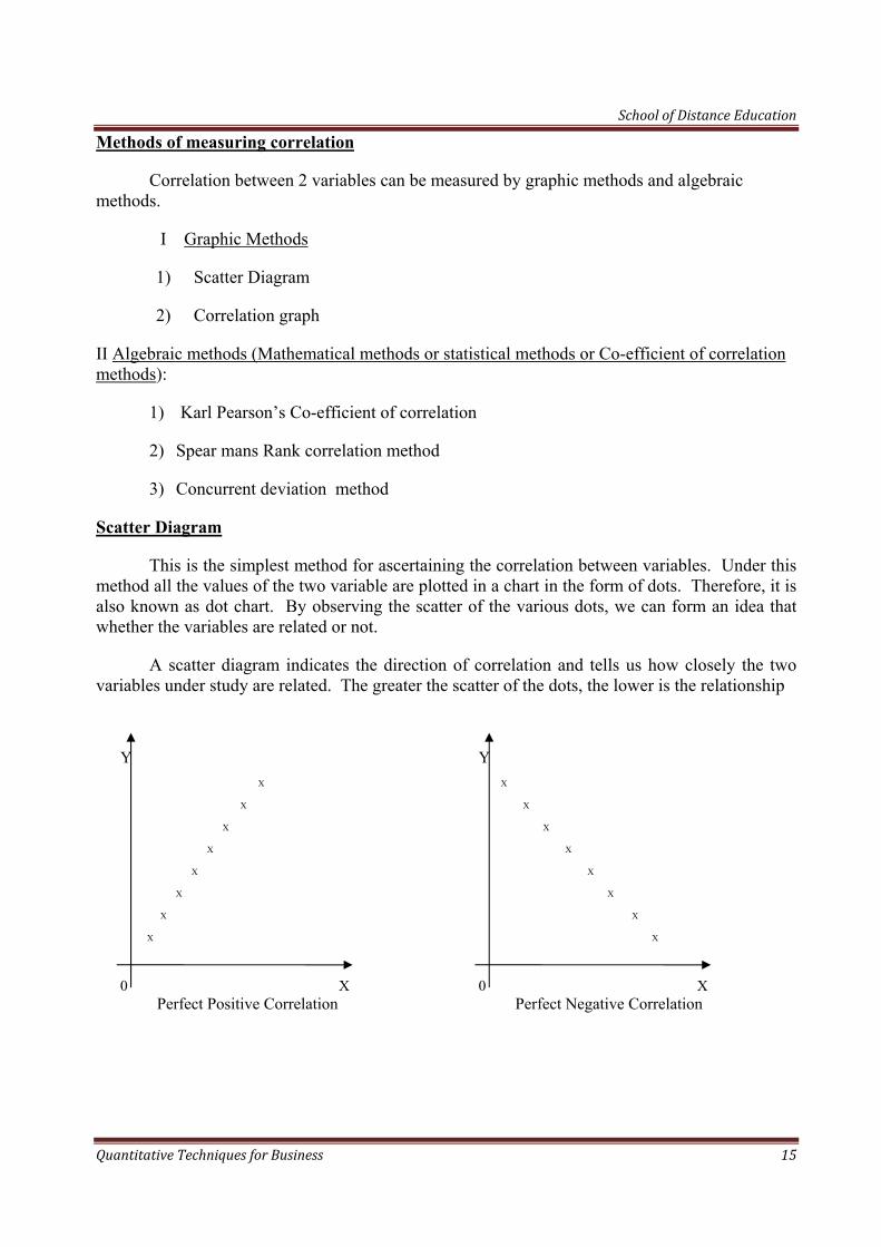
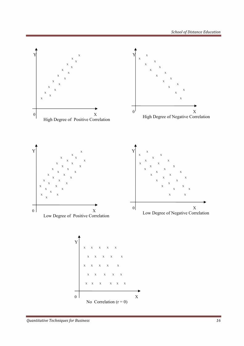
Scatter Diagram
This is the simplest method for ascertaining the correlation between variables. Under this method all the values of the two variable are plotted in a chart in the form of dots. Therefore, it is also known as dot chart. By observing the scatter of the various dots, we can form an idea that whether the variables are related or not.
A scatter diagram indicates the direction of correlation and tells us how closely the two variables under study are related. The greater the scatter of the dots, the lower is the relationship
Y X
X
X
X
X
X
X
X
0 X
Perfect Positive Correlation
Y X
X
X
X
X
X
X
X
0 X
Perfect Negative Correlation
School of Distance Education
Quantitative Techniques for Business 16
Y X X X X X X X X X X X X X X X X
0 X
High Degree of Positive Correlation
Y X X X X X X X X X X X X X X X
0 X
High Degree of Negative Correlation
Y X X X X X X X X X X X X X X X X X X X X X X X X X X X X X X
0 X
Low Degree of Positive Correlation
Y X X X X X X X X X X X X X X X X X X X X X X X X X X X
0 X
Low Degree of Negative Correlation
Y
X X X X X
X X X X X
X X X X X
X X X X X
X X X X X X
0 X
No Correlation (r = 0)
School of Distance Education
Quantitative Techniques for Business 17
Merits of Scatter Diagram method
1. It is a simple method of studying correlation between variables.
2. It is a non-mathematical method of studying correlation between the variables. It does not require any mathematical calculations.
3. It is very easy to understand. It gives an idea about the correlation between variables even to a layman.
4. It is not influenced by the size of extreme items.
5. Making a scatter diagram is, usually, the first step in investigating the relationship between two variables.
Demerits of Scatter diagram method
1. It gives only a rough idea about the correlation between variables.
2. The numerical measurement of correlation co-efficient cannot be calculated under this method.
3. It is not possible to establish the exact degree of relationship between the variables.
Correlation graph Method
Under correlation graph method the individual values of the two variables are plotted on a graph paper. Then dots relating to these variables are joined separately so as to get two curves. By examining the direction and closeness of the two curves, we can infer whether the variables are related or not. If both the curves are moving in the same direction( either upward or downward) correlation is said to be positive. If the curves are moving in the opposite directions, correlation is said to be negative.
Merits of Correlation Graph Method
1. This is a simple method of studying relationship between the variable
2. This does not require mathematical calculations.
3. This method is very easy to understand
Demerits of correlation graph method:
1. A numerical value of correlation cannot be calculated.
2. It is only a pictorial presentation of the relationship between variables.
3. It is not possible to establish the exact degree of relationship between the variables.
Karl Pearson’s Co-efficient of Correlation
Karl Pearson’s Coefficient of Correlation is the most popular method among the algebraic methods for measuring correlation. This method was developed by Prof. Karl Pearson in 1896. It is also called product moment correlation coefficient.

School of Distance Education
Quantitative Techniques for Business 18
Pearson’s coefficient of correlation is defined as the ratio of the covariance between X and Y to the product of their standard deviations. This is denoted by ‘r’ or rxy
r = Covariance of X and Y
(SD of X) x (SD of Y)
Interpretation of Co-efficient of Correlation
Pearson’s Co-efficient of correlation always lies between +1 and -1. The following general rules will help to interpret the Co-efficient of correlation:
1. When r - +1, It means there is perfect positive relationship between variables.
2. When r = -1, it means there is perfect negative relationship between variables.
3. When r = 0, it means there is no relationship between the variables.
4. When ‘r’ is closer to +1, it means there is high degree of positive correlation between variables.
5. When ‘r’ is closer to – 1, it means there is high degree of negative correlation between variables.
6. When ‘r’ is closer to ‘O’, it means there is less relationship between variables.
Properties of Pearson’s Co-efficient of Correlation
1. If there is correlation between variables, the Co-efficient of correlation lies between +1 and -1.
2. If there is no correlation, the coefficient of correlation is denoted by zero (ie r=0)
3. It measures the degree and direction of change
4. If simply measures the correlation and does not help to predict cansation.
5. It is the geometric mean of two regression co-efficients.
i.e r = ·
Computation of Pearson’s Co-efficient of correlation:
Pearson’s correlation co-efficient can be computed in different ways. They are:
a Arithmetic mean method
b Assumed mean method
c Direct method
Arithmetic mean method:-
Under arithmetic mean method, co-efficient of correlation is calculated by taking actual mean.
School of Distance Education
Quantitative Techniques for Business 19
r =
or
r = whereas x-x- and y=y-
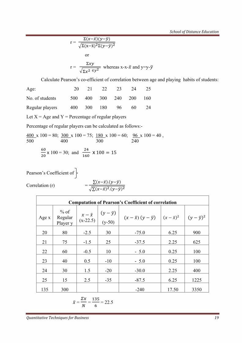
Calculate Pearson’s co-efficient of correlation between age and playing habits of students:
Age: 20 21 22 23 24 25
No. of students 500 400 300 240 200 160
Regular players 400 300 180 96 60 24
Let X = Age and Y = Percentage of regular players
Percentage of regular players can be calculated as follows:-
400 x 100 = 80; 300 x 100 = 75; 180 x 100 = 60; 96 x 100 = 40 , 500 400 300 240
100 = 30; and 100 15
Pearson’s Coefficient of
Correlation (r) = ∑ .∑ .
Computation of Pearson’s Coefficient of correlation
Age x % of
Regular Player y
(x-22.5)
(y-50) )
20 80 -2.5 30 -75.0 6.25 900
21 75 -1.5 25 -37.5 2.25 625
22 60 -0.5 10 - 5.0 0.25 100
23 40 0.5 -10 - 5.0 0.25 100
24 30 1.5 -20 -30.0 2.25 400
25 15 2.5 -35 -87.5 6.25 1225
135 300 -240 17.50 3350
= = = 22.5
School of Distance Education
Quantitative Techniques for Business 20
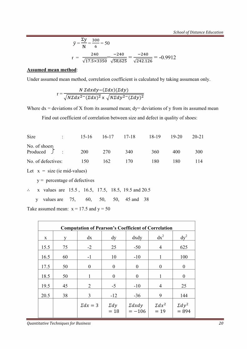
= = = 50
r = √ .
=√ ,
= √ .
= -0.9912
Assumed mean method:
Under assumed mean method, correlation coefficient is calculated by taking assumean only.
r =
Where dx = deviations of X from its assumed mean; dy= deviations of y from its assumed mean
Find out coefficient of correlation between size and defect in quality of shoes:
Size : 15-16 16-17 17-18 18-19 19-20 20-21
No. of shoes Produced : 200 270 340 360 400 300
No. of defectives: 150 162 170 180 180 114
Let x = size (ie mid-values)
y = percentage of defectives
x values are 15.5 , 16.5, 17.5, 18.5, 19.5 and 20.5
y values are 75, 60, 50, 50, 45 and 38
Take assumed mean: x = 17.5 and y = 50
Computation of Pearson’s Coefficient of Correlation
x y dx dy dxdy dx2 dy2
15.5 75 -2 25 -50 4 625
16.5 60 -1 10 -10 1 100
17.5 50 0 0 0 0 0
18.5 50 1 0 0 1 0
19.5 45 2 -5 -10 4 25
20.5 38 3 -12 -36 9 144
3 18 106 19
894
School of Distance Education
Quantitative Techniques for Business 21
r =
√
r =
=
=
= .
= -0.9485
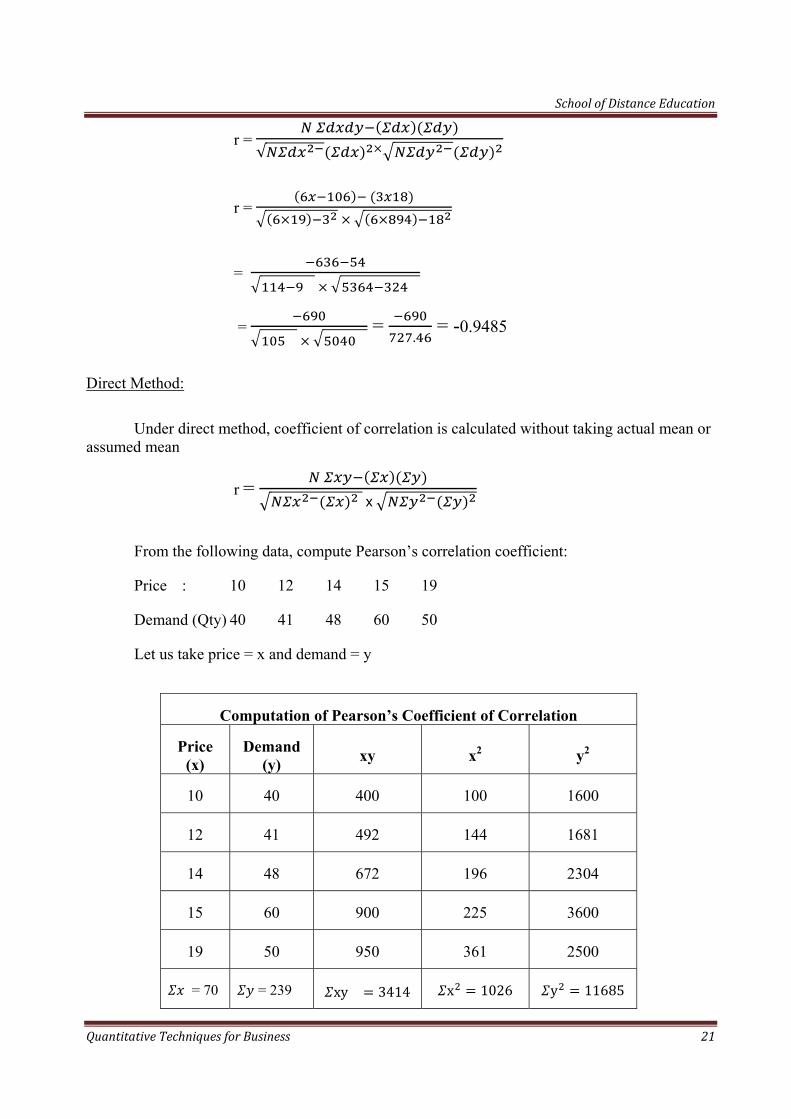
Direct Method:
Under direct method, coefficient of correlation is calculated without taking actual mean or assumed mean
r =
From the following data, compute Pearson’s correlation coefficient:
Price : 10 12 14 15 19
Demand (Qty) 40 41 48 60 50
Let us take price = x and demand = y
Computation of Pearson’s Coefficient of Correlation
Price (x)
Demand (y) xy x2 y2
10 40 400 100 1600
12 41 492 144 1681
14 48 672 196 2304
15 60 900 225 3600
19 50 950 361 2500
= 70 = 239 xy 3414 x 1026 y 11685
School of Distance Education
Quantitative Techniques for Business 22
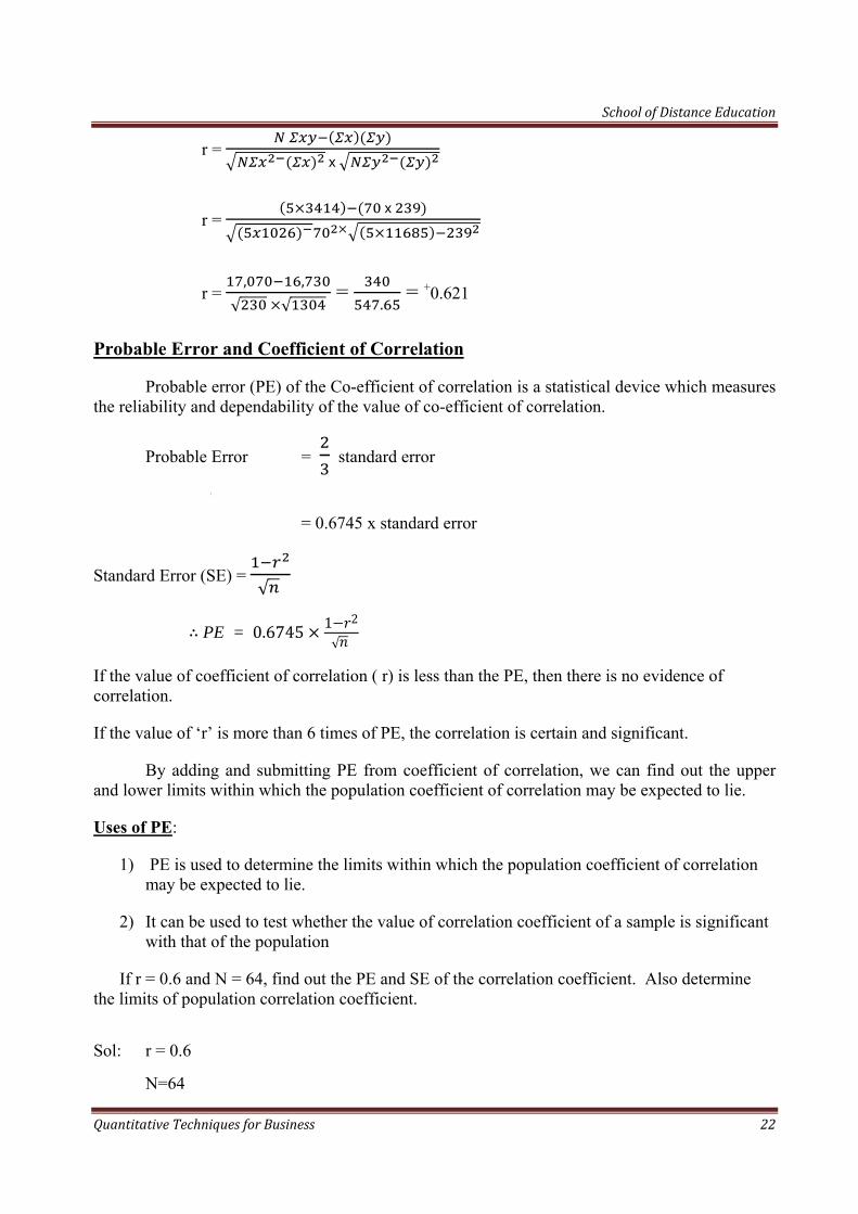
r =
r =
r = , ,
√ √ =
. = +0.621
Probable Error and Coefficient of Correlation
Probable error (PE) of the Co-efficient of correlation is a statistical device which measures the reliability and dependability of the value of co-efficient of correlation.
Probable Error = standard error
[
= 0.6745 x standard error
Standard Error (SE) = √
PE = 0.6745 1 2
√
If the value of coefficient of correlation ( r) is less than the PE, then there is no evidence of correlation.
If the value of ‘r’ is more than 6 times of PE, the correlation is certain and significant.
By adding and submitting PE from coefficient of correlation, we can find out the upper and lower limits within which the population coefficient of correlation may be expected to lie.
Uses of PE:
1) PE is used to determine the limits within which the population coefficient of correlation may be expected to lie.
2) It can be used to test whether the value of correlation coefficient of a sample is significant with that of the population
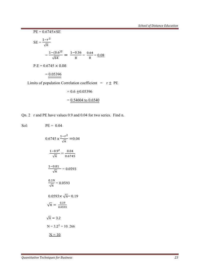
If r = 0.6 and N = 64, find out the PE and SE of the correlation coefficient. Also determine the limits of population correlation coefficient.
Sol: r = 0.6
N=64
School of Distance Education
Quantitative Techniques for Business 23
PE = 0.6745 SE
SE = √
= .√ .
= .
= 0.08
P.E = 0.6745 0.08
= 0.05396
Limits of population Correlation coefficient = r PE
= 0.6 0.05396
= 0.54604 to 0.6540
Qn. 2 r and PE have values 0.9 and 0.04 for two series. Find n.
Sol: PE = 0.04
0.6745 √
0.04
.√
= ..
.√
= 0.0593
.√
= 0.0593
0.0593 √ = 0.19
√ ..
√ 3.2
N = 3.2 = 10. 266
N = 10
School of Distance Education
Quantitative Techniques for Business 24
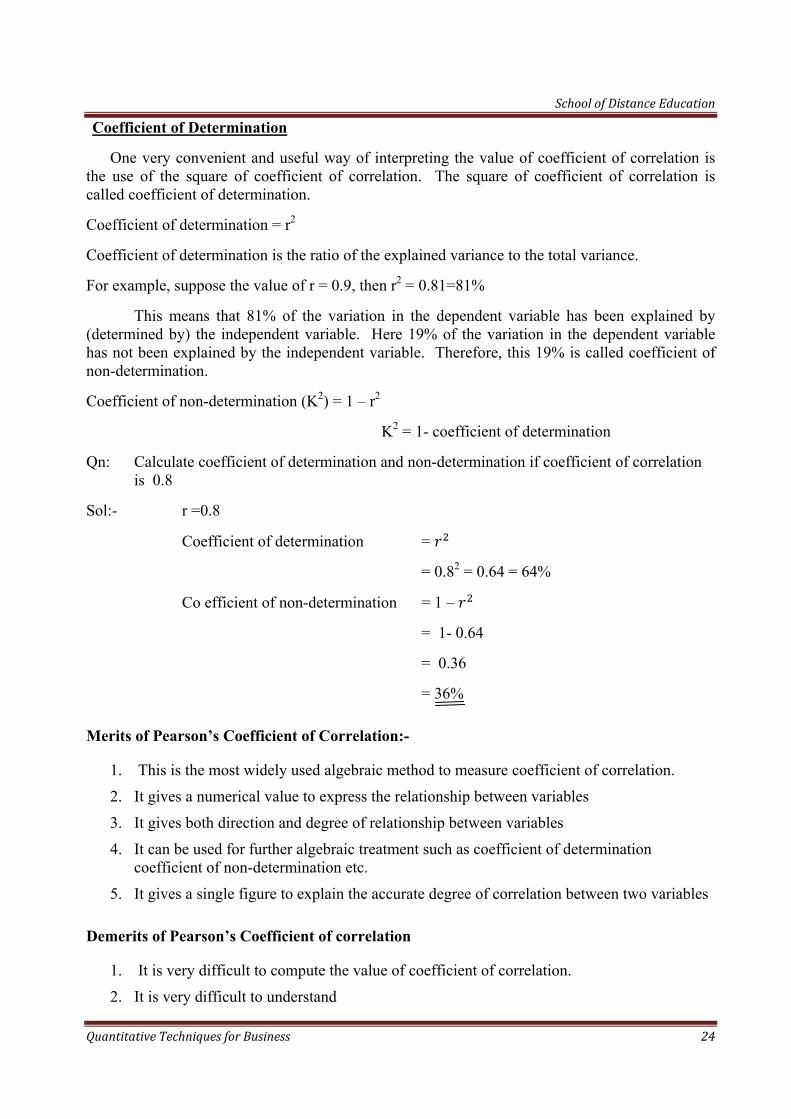
Coefficient of Determination
One very convenient and useful way of interpreting the value of coefficient of correlation is the use of the square of coefficient of correlation. The square of coefficient of correlation is called coefficient of determination.
Coefficient of determination = r2
Coefficient of determination is the ratio of the explained variance to the total variance.
For example, suppose the value of r = 0.9, then r2 = 0.81=81%
This means that 81% of the variation in the dependent variable has been explained by (determined by) the independent variable. Here 19% of the variation in the dependent variable has not been explained by the independent variable. Therefore, this 19% is called coefficient of non-determination.
Coefficient of non-determination (K2) = 1 – r2
K2 = 1- coefficient of determination
Qn: Calculate coefficient of determination and non-determination if coefficient of correlation is 0.8
Sol:- r =0.8
Coefficient of determination =
= 0.82 = 0.64 = 64%
Co efficient of non-determination = 1 –
= 1- 0.64
= 0.36
= 36%
Merits of Pearson’s Coefficient of Correlation:-
1. This is the most widely used algebraic method to measure coefficient of correlation.
2. It gives a numerical value to express the relationship between variables
3. It gives both direction and degree of relationship between variables
4. It can be used for further algebraic treatment such as coefficient of determination coefficient of non-determination etc.
5. It gives a single figure to explain the accurate degree of correlation between two variables
Demerits of Pearson’s Coefficient of correlation
1. It is very difficult to compute the value of coefficient of correlation.
2. It is very difficult to understand

School of Distance Education
Quantitative Techniques for Business 25
3. It requires complicated mathematical calculations
4. It takes more time
5. It is unduly affected by extreme items
6. It assumes a linear relationship between the variables. But in real life situation, it may not be so.
Spearman’s Rank Correlation Method
Pearson’s coefficient of correlation method is applicable when variables are measured in quantitative form. But there were many cases where measurement is not possible because of the qualitative nature of the variable. For example, we cannot measure the beauty, morality, intelligence, honesty etc in quantitative terms. However it is possible to rank these qualitative characteristics in some order.
The correlation coefficient obtained from ranks of the variables instead of their quantitative measurement is called rank correlation. This was developed by Charles Edward Spearman in 1904.
Spearman’s coefficient correlation (R) = 1-
Where D = difference of ranks between the two variables
N = number of pairs
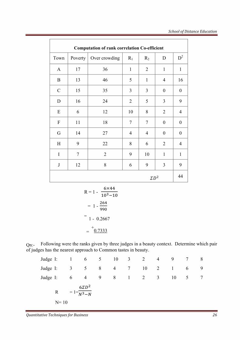
Qn: Find the rank correlation coefficient between poverty and overcrowding from the information given below:
Town: A B C D E F G H I J
Poverty: 17 13 15 16 6 11 14 9 7 12
Over crowing: 36 46 35 24 12 18 27 22 2 8
Sol: Here ranks are not given. Hence we have to assign ranks
R = 1-
N = 10
School of Distance Education
Quantitative Techniques for Business 26
Computation of rank correlation Co-efficient
Town Poverty Over crowding R1 R2 D D2
A 17 36 1 2 1 1
B 13 46 5 1 4 16
C 15 35 3 3 0 0
D 16 24 2 5 3 9
E 6 12 10 8 2 4
F 11 18 7 7 0 0
G 14 27 4 4 0 0
H 9 22 8 6 2 4
I 7 2 9 10 1 1
J 12 8 6 9 3 9
44
R = 1 -
= 1 - = 1 - 0.2667
= +
0.7333
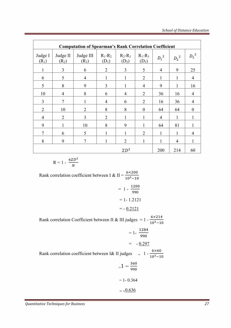
Qn:- Following were the ranks given by three judges in a beauty context. Determine which pair of judges has the nearest approach to Common tastes in beauty.
Judge I: 1 6 5 10 3 2 4 9 7 8
Judge I: 3 5 8 4 7 10 2 1 6 9
Judge I: 6 4 9 8 1 2 3 10 5 7
R = 1=
N= 10
School of Distance Education
Quantitative Techniques for Business 27
Computation of Spearman’s Rank Correlation Coefficient
Judge I (R1)
Judge II (R2)
Judge III (R3)
R1-R2 (D1)
R2-R3 (D2)
R1-R3 (D3)
1 3 6 2 3 5 4 9 25
6 5 4 1 1 2 1 1 4
5 8 9 3 1 4 9 1 16
10 4 8 6 4 2 36 16 4
3 7 1 4 6 2 16 36 4
2 10 2 8 8 0 64 64 0
4 2 3 2 1 1 4 1 1
9 1 10 8 9 1 64 81 1
7 6 5 1 1 2 1 1 4
8 9 7 1 2 1 1 4 1
200 214 60
R = 1 -
Rank correlation coefficient between I & II =
= 1 -
= 1- 1.2121
= - 0.2121
Rank correlation Coefficient between II & III judges = 1 -
= 1-
= - 0.297
Rank correlation coefficient between I& II judges = 1 -
=1
= 1- 0.364
= +0.636
School of Distance Education
Quantitative Techniques for Business 28
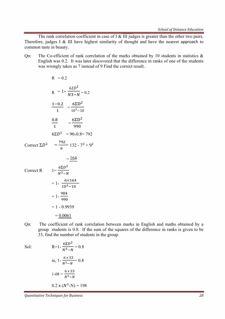
The rank correlation coefficient in case of I & III judges is greater than the other two pairs. Therefore, judges I & III have highest similarity of thought and have the nearest approach to common taste in beauty.
Qn: The Co-efficient of rank correlation of the marks obtained by 10 students in statistics & English was 0.2. It was later discovered that the difference in ranks of one of the students was wrongly takes as 7 instead of 9 Find the correct result.
R = 0.2
R = 1- 62
= 0.2
. = 103 10
. =
6Σ = 90 0.8= 792
Correct Σ =
= 132 - 7 + 9
= 164
Correct R 1=
= 1-
= 1-
= 1 - 0.9939
= 0.0061
Qn: The coefficient of rank correlation between marks in English and maths obtained by a group students is 0.8. If the sum of the squares of the difference in ranks is given to be 33, find the number of students in the group.
Sol: R=1- = 0.8
ie, 1-
= 0.8
1-08 =
0.2 ( -N) = 198
School of Distance Education
Quantitative Techniques for Business 29
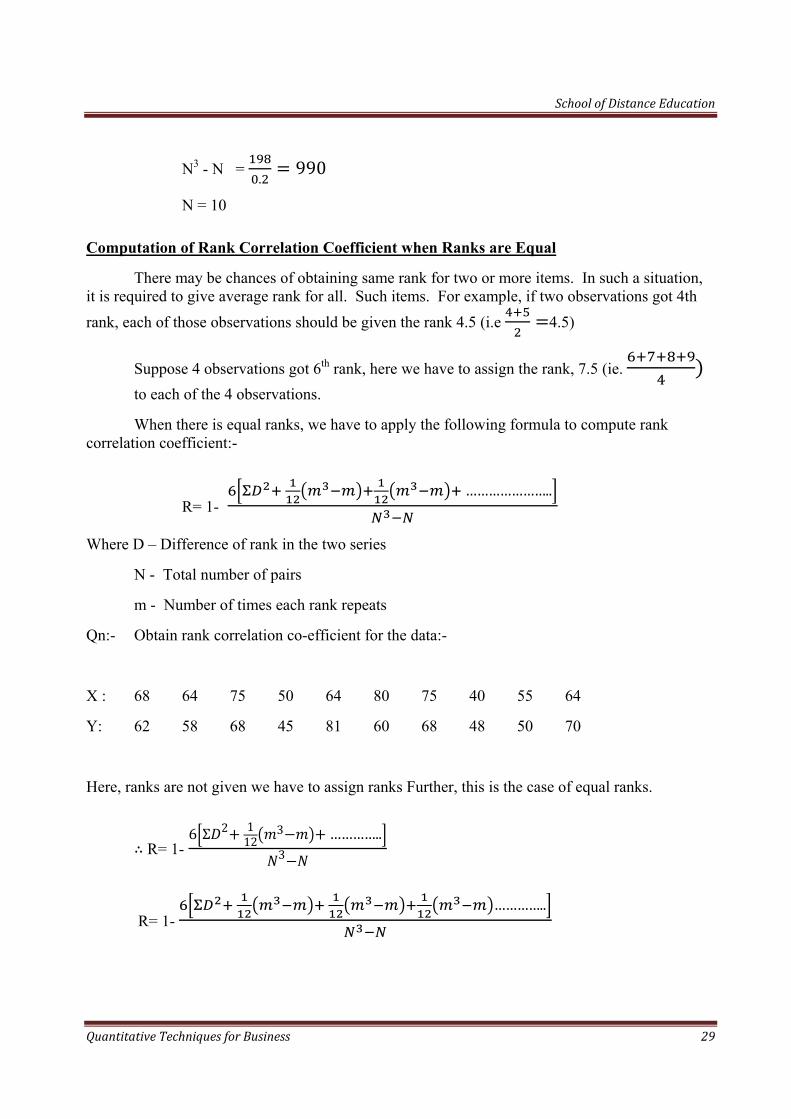
N3 - N = .
990
N = 10
Computation of Rank Correlation Coefficient when Ranks are Equal
There may be chances of obtaining same rank for two or more items. In such a situation, it is required to give average rank for all. Such items. For example, if two observations got 4th rank, each of those observations should be given the rank 4.5 (i.e 4.5)
Suppose 4 observations got 6th rank, here we have to assign the rank, 7.5 (ie. to each of the 4 observations.
When there is equal ranks, we have to apply the following formula to compute rank correlation coefficient:-
R= 1- …………………..
Where D – Difference of rank in the two series
N - Total number of pairs
m - Number of times each rank repeats
Qn:- Obtain rank correlation co-efficient for the data:-
X : 68 64 75 50 64 80 75 40 55 64
Y: 62 58 68 45 81 60 68 48 50 70
Here, ranks are not given we have to assign ranks Further, this is the case of equal ranks.
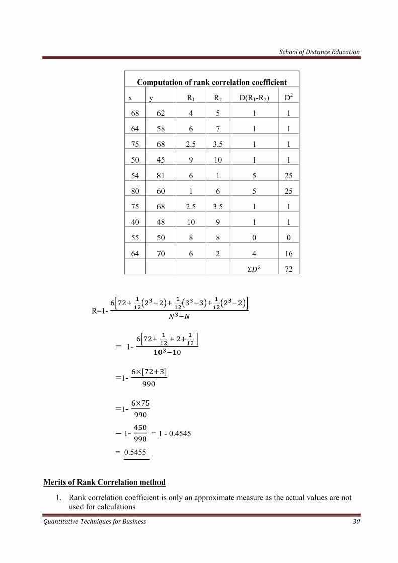
R= 1- 6 Σ 2 112
3 …………..3
R= 1- …………..
School of Distance Education
Quantitative Techniques for Business 30
Computation of rank correlation coefficient
x y R1 R2 D(R1-R2) D2
68 62 4 5 1 1
64 58 6 7 1 1
75 68 2.5 3.5 1 1
50 45 9 10 1 1
54 81 6 1 5 25
80 60 1 6 5 25
75 68 2.5 3.5 1 1
40 48 10 9 1 1
55 50 8 8 0 0
64 70 6 2 4 16
Σ 72
R=1-
= 1-
=1-
=1-
= 1- = 1 - 0.4545
= 0.5455
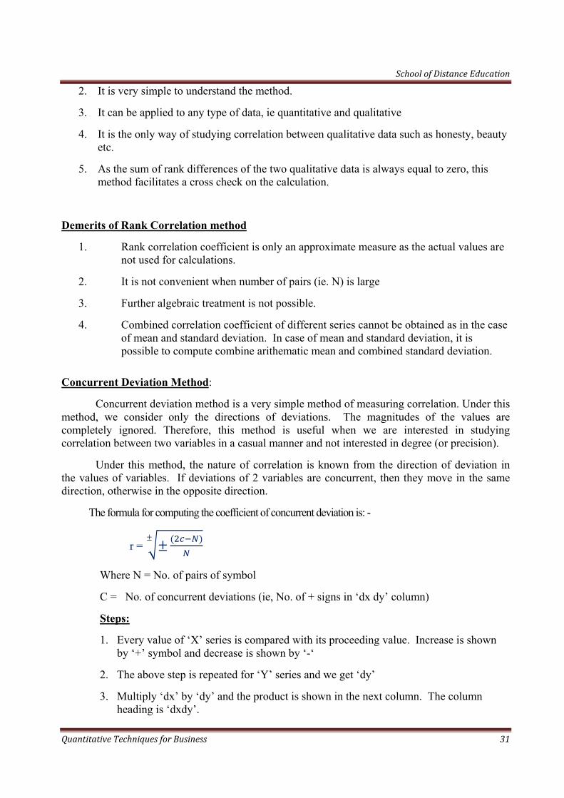
Merits of Rank Correlation method
1. Rank correlation coefficient is only an approximate measure as the actual values are not used for calculations
School of Distance Education
Quantitative Techniques for Business 31
2. It is very simple to understand the method.
3. It can be applied to any type of data, ie quantitative and qualitative
4. It is the only way of studying correlation between qualitative data such as honesty, beauty etc.
5. As the sum of rank differences of the two qualitative data is always equal to zero, this method facilitates a cross check on the calculation.
Demerits of Rank Correlation method
1. Rank correlation coefficient is only an approximate measure as the actual values are not used for calculations.
2. It is not convenient when number of pairs (ie. N) is large
3. Further algebraic treatment is not possible.
4. Combined correlation coefficient of different series cannot be obtained as in the case of mean and standard deviation. In case of mean and standard deviation, it is possible to compute combine arithematic mean and combined standard deviation.
Concurrent Deviation Method:
Concurrent deviation method is a very simple method of measuring correlation. Under this method, we consider only the directions of deviations. The magnitudes of the values are completely ignored. Therefore, this method is useful when we are interested in studying correlation between two variables in a casual manner and not interested in degree (or precision).
Under this method, the nature of correlation is known from the direction of deviation in the values of variables. If deviations of 2 variables are concurrent, then they move in the same direction, otherwise in the opposite direction.
The formula for computing the coefficient of concurrent deviation is: -
r =
Where N = No. of pairs of symbol
C = No. of concurrent deviations (ie, No. of + signs in ‘dx dy’ column)
Steps:
1. Every value of ‘X’ series is compared with its proceeding value. Increase is shown by ‘+’ symbol and decrease is shown by ‘-‘
2. The above step is repeated for ‘Y’ series and we get ‘dy’
3. Multiply ‘dx’ by ‘dy’ and the product is shown in the next column. The column heading is ‘dxdy’.
School of Distance Education
Quantitative Techniques for Business 32
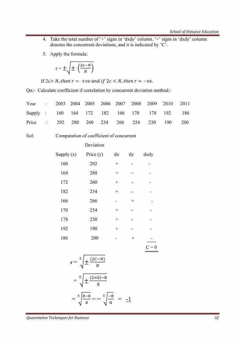
4. Take the total number of ‘+’ signs in ‘dxdy’ column. ‘+’ signs in ‘dxdy’ column denotes the concurrent deviations, and it is indicated by ‘C’.
5. Apply the formula:
r =
If 2c , 2 , .
Qn:- Calculate coefficient if correlation by concurrent deviation method:-
Year : 2003 2004 2005 2006 2007 2008 2009 2010 2011
Supply : 160 164 172 182 166 170 178 192 186
Price : 292 280 260 234 266 254 230 190 200
Sol: Computation of coefficient of concurrent
Deviation
Supply (x) Price (y) dx dy dxdy
160 292 + - -
164 280 + - -
172 260 + - -
182 234 + - -
166 266 - + -
170 254 + - -
178 230 + - -
192 190 + - -
186 200 - + -
C = 0
r =
=
= = = = -1
School of Distance Education
Quantitative Techniques for Business 33
Merits of concurrent deviation method:
1. It is very easy to calculate coefficient of correlation
2. It is very simple understand the method
3. When the number of items is very large, this method may be used to form quick idea about the degree of relationship
4. This method is more suitable, when we want to know the type of correlation (ie, whether positive or negative).
Demerits of concurrent deviation method:
1. This method ignores the magnitude of changes. Ie. Equal weight is give for small and big changes.
2. The result obtained by this method is only a rough indicator of the presence or absence of correlation
3. Further algebraic treatment is not possible
4. Combined coefficient of concurrent deviation of different series cannot be found as in the case of arithmetic mean and standard deviation.
School of Distance Education
Quantitative Techniques for Business 34
CHAPTER - 3
REGRESSION ANALYSIS
Introduction:-
Correlation analysis analyses whether two variables are correlated or not. After having established the fact that two variables are closely related, we may be interested in estimating the value of one variable, given the value of another. Hence, regression analysis means to analyse the average relationship between two variables and thereby provides a mechanism for estimation or predication or forecasting.
The term ‘Regression” was firstly used by Sir Francis Galton in 1877. The dictionary meaning of the term ‘regression” is “stepping back” to the average.
Definition:
“Regression is the measure of the average relationship between two or more variables in terms of the original units of the date”.
“Regression analysis is an attempt to establish the nature of the relationship between variables-that is to study the functional relationship between the variables and thereby provides a mechanism for prediction or forecasting”.
It is clear from the above definitions that Regression Analysis is a statistical device with the help of which we are able to estimate the unknown values of one variable from known values of another variable. The variable which is used to predict the another variable is called independent variable (explanatory variable) and, the variable we are trying to predict is called dependent variable (explained variable).
The dependent variable is denoted by X and the independent variable is denoted by Y.
The analysis used in regression is called simple linear regression analysis. It is called simple because three is only one predictor (independent variable). It is called linear because, it is assumed that there is linear relationship between independent variable and dependent variable.
Types of Regression:-
There are two types of regression. They are linear regression and multiple regression.
Linear Regression:
It is a type of regression which uses one independent variable to explain and/or predict the dependent variable.
Multiple Regression:
It is a type of regression which uses two or more independent variable to explain and/or predict the dependent variable.
School of Distance Education
Quantitative Techniques for Business 35
Regression Lines:
Regression line is a graphic technique to show the functional relationship between the two variables X and Y. It is a line which shows the average relationship between two variables X and Y.
If there is perfect positive correlation between 2 variables, then the two regression lines are winding each other and to give one line. There would be two regression lines when there is no perfect correlation between two variables. The nearer the two regression lines to each other, the higher is the degree of correlation and the farther the regression lines from each other, the lesser is the degree of correlation.
Properties of Regression lines:-
1. The two regression lines cut each other at the point of average of X and average of Y ( i.e X and Y )
2. When r = 1, the two regression lines coincide each other and give one line.
3. When r = 0, the two regression lines are mutually perpendicular.
Regression Equations (Estimating Equations)
Regression equations are algebraic expressions of the regression lines. Since there are two regression lines, therefore two regression equations. They are :-
1. Regression Equation of X on Y:- This is used to describe the variations in the values of X for given changes in Y.
2. Regression Equation of Y on X :- This is used to describe the variations in the value of Y for given changes in X.
Least Square Method of computing Regression Equation:
The method of least square is an objective method of determining the best relationship between the two variables constituting a bivariate data. To find out best relationship means to determine the values of the constants involved in the functional relationship between the two variables. This can be done by the principle of least squares:
The principle of least squares says that the sum of the squares of the deviations between the observed values and estimated values should be the least. In other words, Σ will be the minimum.
With a little algebra and differential calculators we can develop some equations (2 equations in case of a linear relationship) called normal equations. By solving these normal equations, we can find out the best values of the constants.
Regression Equation of Y on X:- Y = a + bx
The normal equations to compute ‘a’ and ‘b’ are: -
Σ Σ
Σ Σ Σ
School of Distance Education
Quantitative Techniques for Business 36
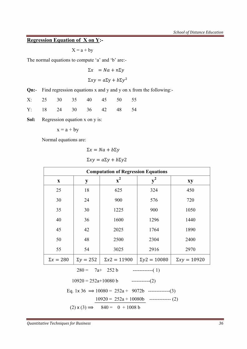
Regression Equation of X on Y:-
X = a + by
The normal equations to compute ‘a’ and ‘b’ are:-
Σ Σ
Σ Σy Σ
Qn:- Find regression equations x and y and y on x from the following:-
X: 25 30 35 40 45 50 55
Y: 18 24 30 36 42 48 54
Sol: Regression equation x on y is:
x = a + by
Normal equations are:
Σ Σ
Σ Σ Σ 2
Computation of Regression Equations
x y x2 y2 xy 25 18 625 324 450
30 24 900 576 720
35 30 1225 900 1050
40 36 1600 1296 1440
45 42 2025 1764 1890
50 48 2500 2304 2400
55 54 3025 2916 2970
Σ 280 Σ 252 Σ 2 11900 Σ 2 10080 Σ 10920
280 = 7a+ 252 b ------------( 1)
10920 = 252a+10080 b -----------(2)
Eq. 1 36 10080 = 252a + 9072b -------------(3)
10920 = 252a + 10080b ------------- (2)
(2) (3) 840 = 0 + 1008 b
School of Distance Education
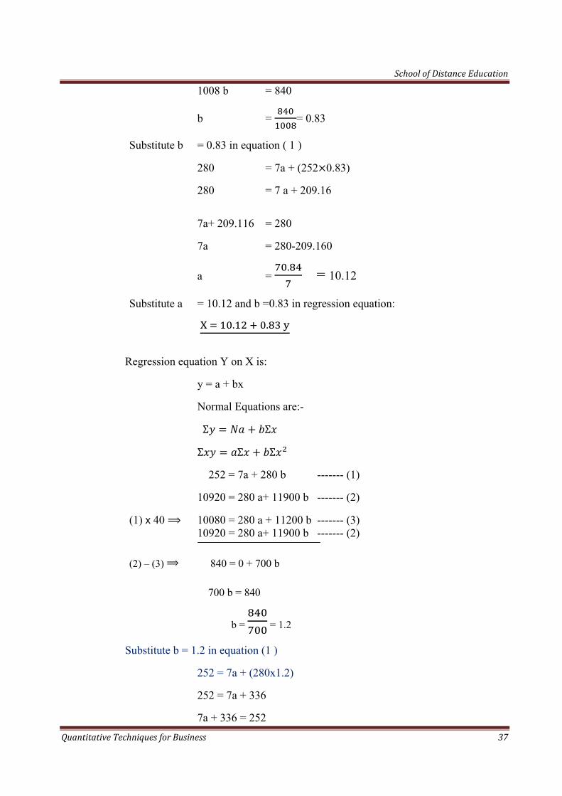
Quantitative Techniques for Business 37
1008 b = 840
b = = 0.83
Substitute b = 0.83 in equation ( 1 )
280 = 7a + (252 0.83)
280 = 7 a + 209.16
7a+ 209.116 = 280
7a = 280-209.160
a = . = 10.12
Substitute a = 10.12 and b =0.83 in regression equation:
. .
Regression equation Y on X is:
y = a + bx
Normal Equations are:-
Σ Σ
Σ Σ Σ
252 = 7a + 280 b ------- (1)
10920 = 280 a+ 11900 b ------- (2)
(1) 40 10080 = 280 a + 11200 b ------- (3) 10920 = 280 a+ 11900 b ------- (2)
(2) – (3) 840 = 0 + 700 b
700 b = 840
b = = 1.2
Substitute b = 1.2 in equation (1 )
252 = 7a + (280x1.2)
252 = 7a + 336
7a + 336 = 252
School of Distance Education
Quantitative Techniques for Business 38
7a = 252 – 336 = -84
a = = -12
Substitute a = -12 and b = 1.2 in regression equation
y = -12+1.2x
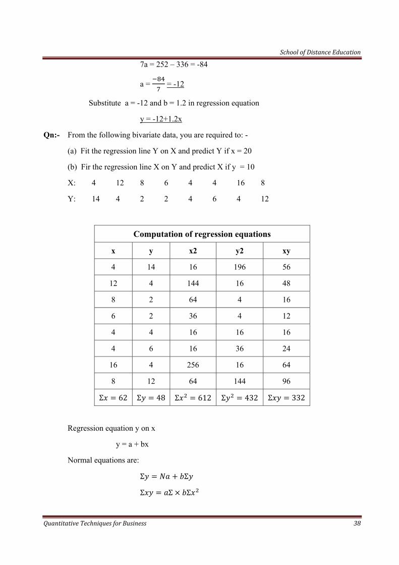
Qn:- From the following bivariate data, you are required to: -
(a) Fit the regression line Y on X and predict Y if x = 20
(b) Fir the regression line X on Y and predict X if y = 10
X: 4 12 8 6 4 4 16 8
Y: 14 4 2 2 4 6 4 12
Computation of regression equations
x y x2 y2 xy
4 14 16 196 56
12 4 144 16 48
8 2 64 4 16
6 2 36 4 12
4 4 16 16 16
4 6 16 36 24
16 4 256 16 64
8 12 64 144 96
Σ 62 Σ 48 Σ 612 Σ 432 Σ 332
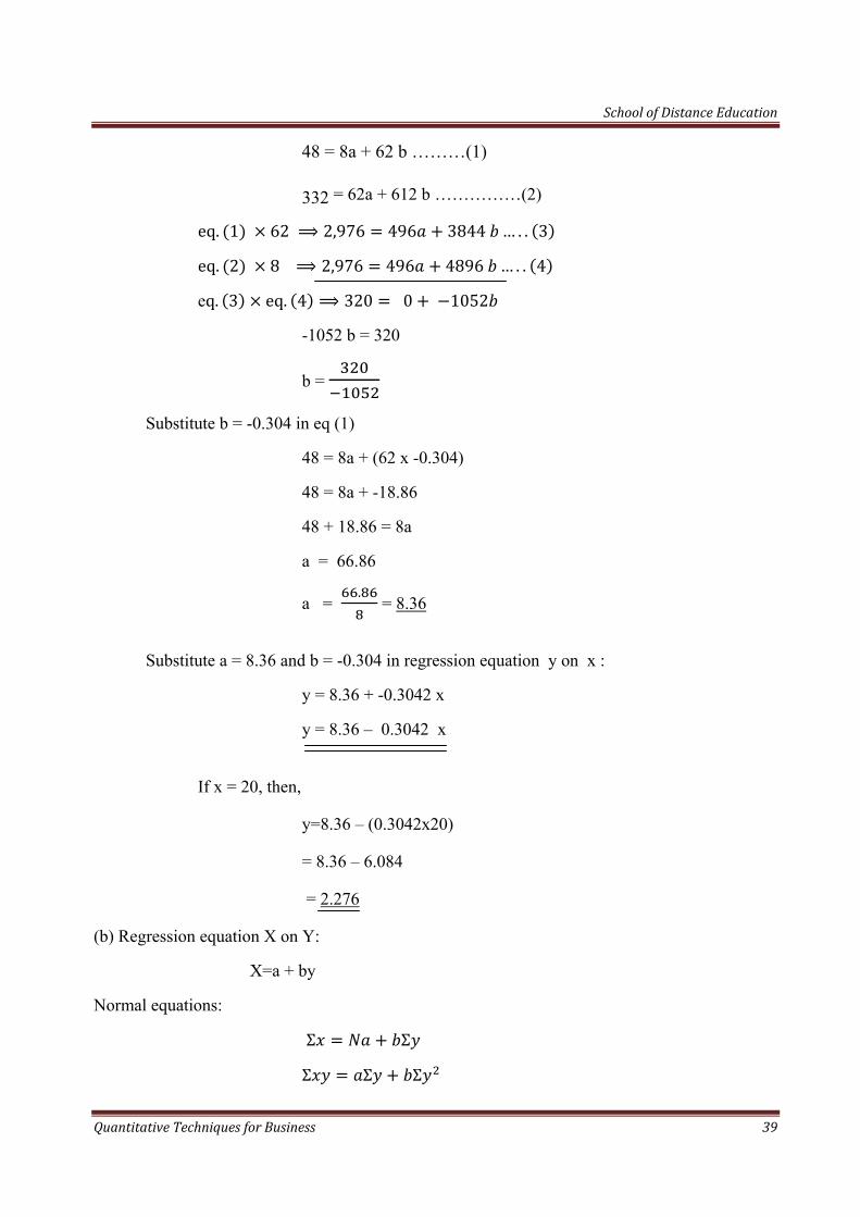
Regression equation y on x
y = a + bx
Normal equations are:
Σ Σ
Σ Σ Σ
School of Distance Education
Quantitative Techniques for Business 39
48 = 8a + 62 b ………(1)
332 = 62a + 612 b ……………(2)
eq. 1 62 2,976 496 3844 … . . 3
eq. 2 8 2,976 496 4896 … . . 4
eq. 3 eq. 4 320 0 1052
-1052 b = 320
b =
Substitute b = -0.304 in eq (1)
48 = 8a + (62 x -0.304)
48 = 8a + -18.86
48 + 18.86 = 8a
a = 66.86
a = .
= 8.36
Substitute a = 8.36 and b = -0.304 in regression equation y on x :
y = 8.36 + -0.3042 x
y = 8.36 – 0.3042 x
If x = 20, then,
y=8.36 – (0.3042x20)
= 8.36 – 6.084
= 2.276
(b) Regression equation X on Y:
X=a + by
Normal equations:
Σ Σ
Σ Σ Σ
School of Distance Education
Quantitative Techniques for Business 40
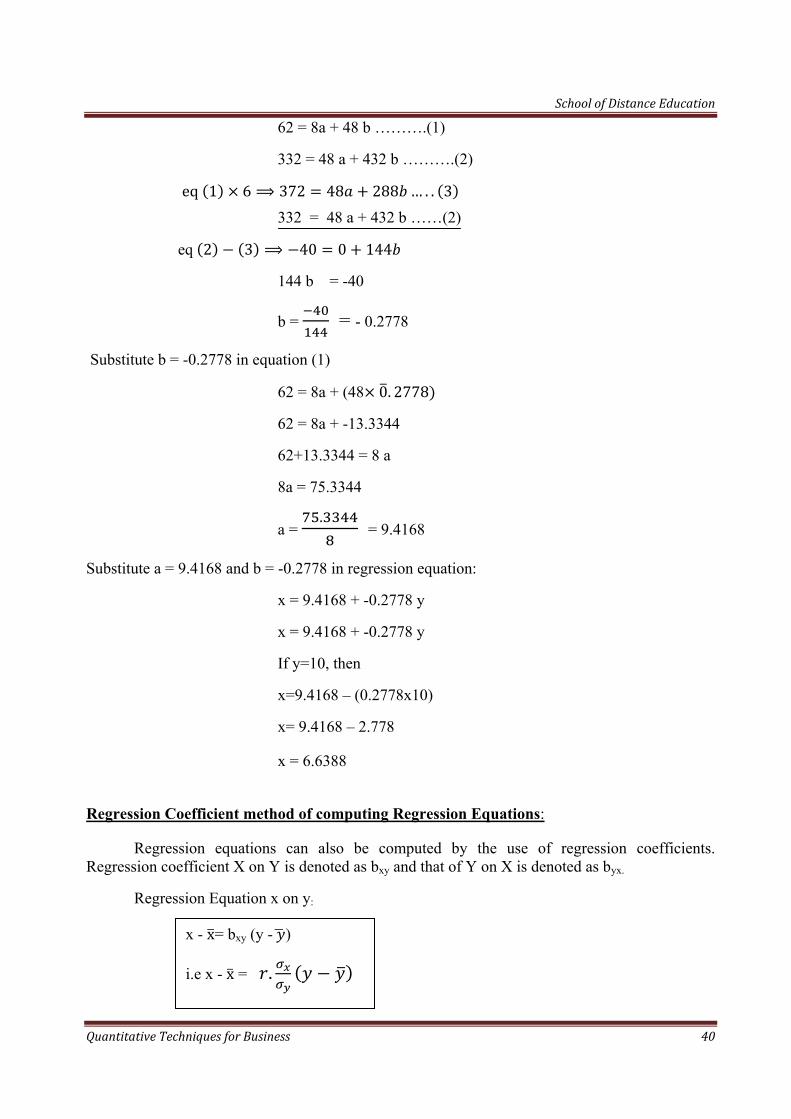
62 = 8a + 48 b ……….(1)
332 = 48 a + 432 b ……….(2)
eq 1 6 372 48 288 … . . 3 332 = 48 a + 432 b ……(2)
eq 2 3 40 0 144
144 b = -40
b = = - 0.2778
Substitute b = -0.2778 in equation (1)
62 = 8a + (48 0. 2778
62 = 8a + -13.3344
62+13.3344 = 8 a
8a = 75.3344
a = . = 9.4168
Substitute a = 9.4168 and b = -0.2778 in regression equation:
x = 9.4168 + -0.2778 y
x = 9.4168 + -0.2778 y
If y=10, then
x=9.4168 – (0.2778x10)
x= 9.4168 – 2.778
x = 6.6388
Regression Coefficient method of computing Regression Equations:
Regression equations can also be computed by the use of regression coefficients. Regression coefficient X on Y is denoted as bxy and that of Y on X is denoted as byx.
Regression Equation x on y:
x - x= bxy (y - )
i.e x - x = .
School of Distance Education
Quantitative Techniques for Business 41
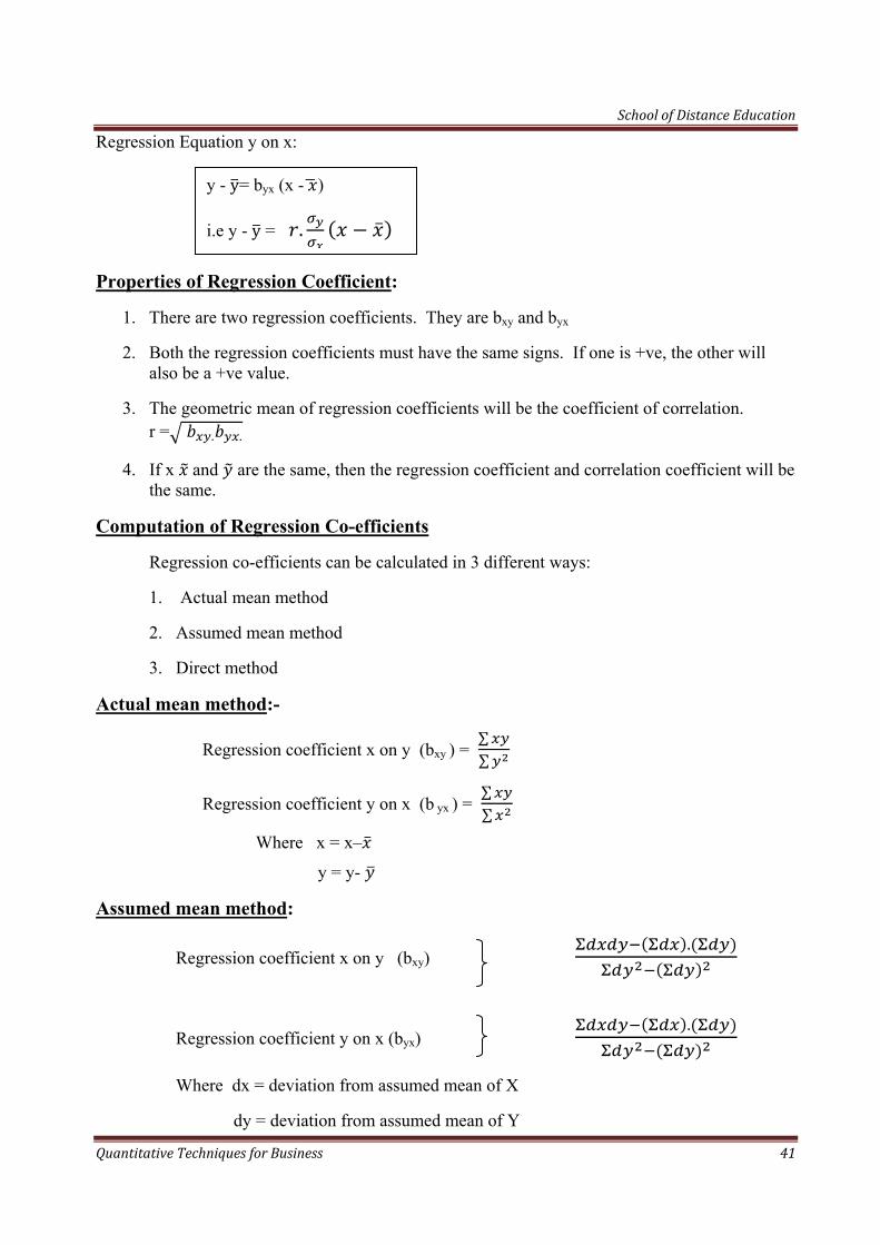
Regression Equation y on x:
Properties of Regression Coefficient:
1. There are two regression coefficients. They are bxy and byx
2. Both the regression coefficients must have the same signs. If one is +ve, the other will also be a +ve value.
3. The geometric mean of regression coefficients will be the coefficient of correlation. r = . .
4. If x and are the same, then the regression coefficient and correlation coefficient will be the same.
Computation of Regression Co-efficients
Regression co-efficients can be calculated in 3 different ways:
1. Actual mean method
2. Assumed mean method
3. Direct method
Actual mean method:-
Regression coefficient x on y (bxy ) = ∑∑
Regression coefficient y on x (b yx ) = ∑∑
Where x = x– y = y-
Assumed mean method:
Regression coefficient x on y (bxy) .
Regression coefficient y on x (byx) .
Where dx = deviation from assumed mean of X
dy = deviation from assumed mean of Y
y - y= byx (x - )
i.e y - y = .
School of Distance Education
Quantitative Techniques for Business 42
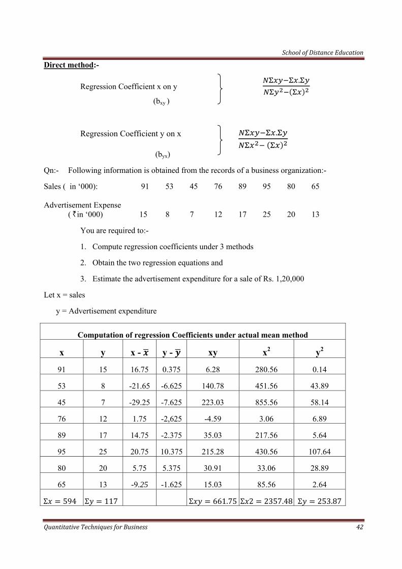
Direct method:-
Regression Coefficient x on y .
(bxy )
Regression Coefficient y on x .
(byx)
Qn:- Following information is obtained from the records of a business organization:-
Sales ( in ‘000): 91 53 45 76 89 95 80 65 Advertisement Expense ( in ‘000) 15 8 7 12 17 25 20 13
You are required to:-
1. Compute regression coefficients under 3 methods
2. Obtain the two regression equations and
3. Estimate the advertisement expenditure for a sale of Rs. 1,20,000
Let x = sales
y = Advertisement expenditure
Computation of regression Coefficients under actual mean method
x y x - y - xy x2 y2
91 15 16.75 0.375 6.28 280.56 0.14
53 8 -21.65 -6.625 140.78 451.56 43.89
45 7 -29.25 -7.625 223.03 855.56 58.14
76 12 1.75 -2,625 -4.59 3.06 6.89
89 17 14.75 -2.375 35.03 217.56 5.64
95 25 20.75 10.375 215.28 430.56 107.64
80 20 5.75 5.375 30.91 33.06 28.89
65 13 -9.25 -1.625 15.03 85.56 2.64
Σ 594 Σ 117 Σ 661.75 Σ 2 2357.48 Σ 253.87
School of Distance Education
Quantitative Techniques for Business 43
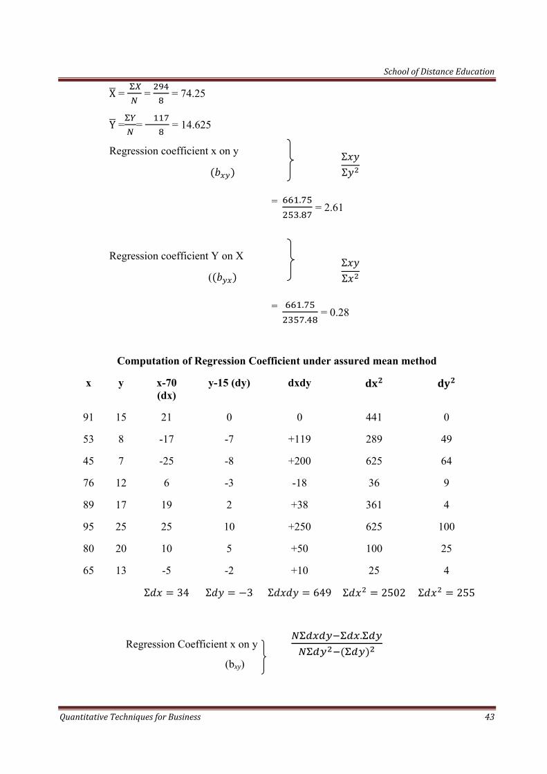
X =
= = 74.25
Y = =
= 14.625
Regression coefficient x on y
ΣΣ
= ..
= 2.61
Regression coefficient Y on X
ΣΣ (
= ..
= 0.28
Computation of Regression Coefficient under assured mean method
x y x-70 (dx)
y-15 (dy) dxdy
91 15 21 0 0 441 0
53 8 -17 -7 +119 289 49
45 7 -25 -8 +200 625 64
76 12 6 -3 -18 36 9
89 17 19 2 +38 361 4
95 25 25 10 +250 625 100
80 20 10 5 +50 100 25
65 13 -5 -2 +10 25 4
Σ 34 Σ 3 Σ 649 Σ 2502 Σ 255
Regression Coefficient x on y .
(bxy)
School of Distance Education
Quantitative Techniques for Business 44
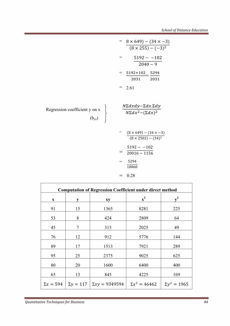
= 8 649 34 38 255 3
= 5192 1022040 9
= =
= 2.61
Regression coefficient y on x .
(byx)
= 8 649 34 38 2502 34
==
5192 10220016 1156
529418860
= 0.28
Computation of Regression Coefficient under direct method
x y xy x2 y2
91 15 1365 8281 225
53 8 424 2809 64
45 7 315 2025 49
76 12 912 5776 144
89 17 1513 7921 289
95 25 2375 9025 625
80 20 1600 6400 400
65 13 845 4225 169
Σ 594 Σ 117 Σ 9349594 Σ 46462 Σ 1965
School of Distance Education
Quantitative Techniques for Business 45
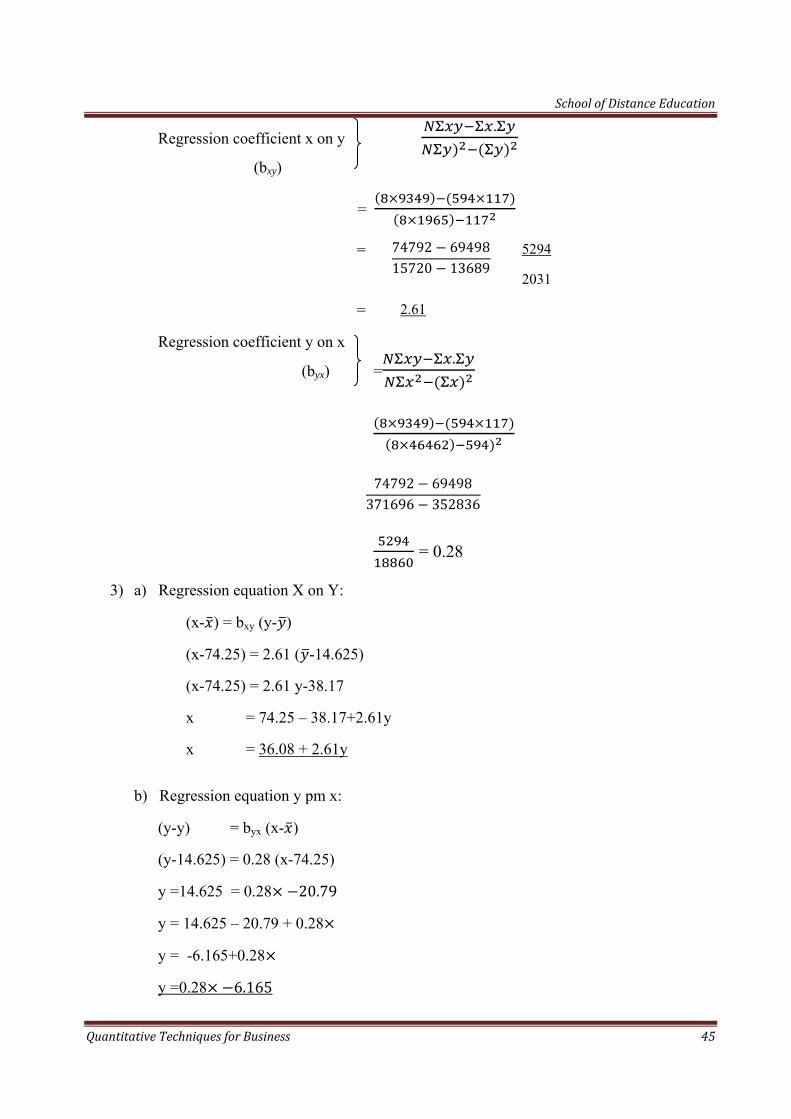
Regression coefficient x on y .
(bxy)
=
= 74792 6949815720 13689
5294
2031
= 2.61
Regression coefficient y on x
(byx) =.
74792 69498371696 352836
= 0.28
3) a) Regression equation X on Y:
(x- ) = bxy (y- )
(x-74.25) = 2.61 ( -14.625)
(x-74.25) = 2.61 y-38.17
x = 74.25 – 38.17+2.61y
x = 36.08 + 2.61y
b) Regression equation y pm x:
(y-y) = byx (x- )
(y-14.625) = 0.28 (x-74.25)
y =14.625 = 0.28 20.79
y = 14.625 – 20.79 + 0.28
y = -6.165+0.28
y =0.28 6.165
School of Distance Education
Quantitative Techniques for Business 46
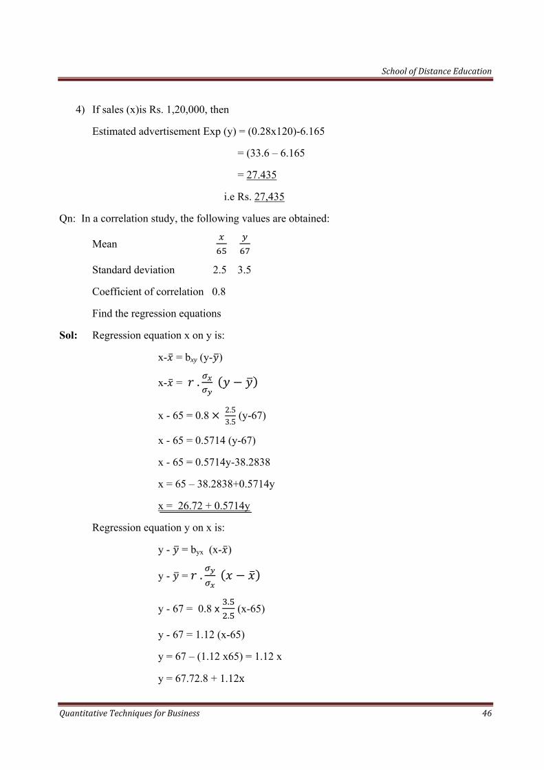
4) If sales (x)is Rs. 1,20,000, then
Estimated advertisement Exp (y) = (0.28x120)-6.165
= (33.6 – 6.165
= 27.435
i.e Rs. 27,435
Qn: In a correlation study, the following values are obtained:
Mean
Standard deviation 2.5 3.5
Coefficient of correlation 0.8
Find the regression equations
Sol: Regression equation x on y is:
x- = bxy (y- )
x- = .
x - 65 = 0.8 2.53.5
(y-67)
x - 65 = 0.5714 (y-67)
x - 65 = 0.5714y-38.2838
x = 65 – 38.2838+0.5714y
x = 26.72 + 0.5714y
Regression equation y on x is:
y - = byx (x- )
y - = .
y - 67 = 0.8 ..
(x-65)
y - 67 = 1.12 (x-65)
y = 67 – (1.12 x65) = 1.12 x
y = 67.72.8 + 1.12x
School of Distance Education
Quantitative Techniques for Business 47
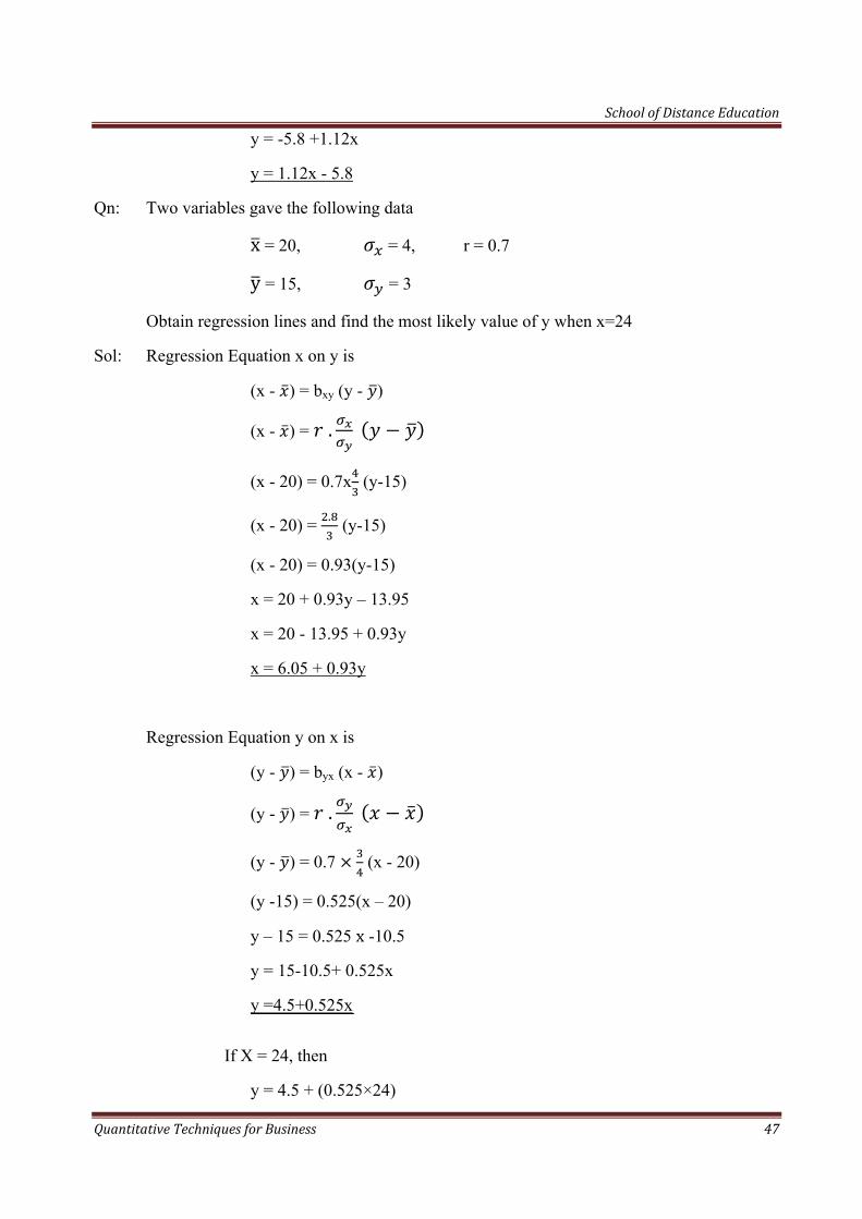
y = -5.8 +1.12x
y = 1.12x - 5.8
Qn: Two variables gave the following data
x = 20, = 4, r = 0.7
y = 15, = 3
Obtain regression lines and find the most likely value of y when x=24
Sol: Regression Equation x on y is
(x - ) = bxy (y - )
(x - ) = .
(x - 20) = 0.7x (y-15)
(x - 20) = . (y-15)
(x - 20) = 0.93(y-15)
x = 20 + 0.93y – 13.95
x = 20 - 13.95 + 0.93y
x = 6.05 + 0.93y
Regression Equation y on x is
(y - ) = byx (x - )
(y - ) = .
(y - ) = 0.7 (x - 20)
(y -15) = 0.525(x – 20)
y – 15 = 0.525 x -10.5
y = 15-10.5+ 0.525x
y =4.5+0.525x
If X = 24, then
y = 4.5 + (0.525×24)
School of Distance Education
Quantitative Techniques for Business 48
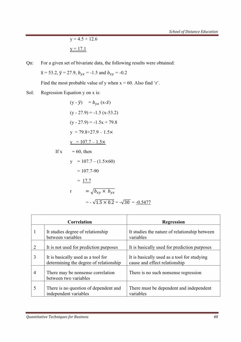
y = 4.5 + 12.6
y = 17.1
Qn: For a given set of bivariate data, the following results were obtained:
x = 53.2, y = 27.9, = -1.5 and = -0.2
Find the most probable value of y when x = 60. Also find ‘r’.
Sol: Regression Equation y on x is:
(y - ) = (x- )
(y - 27.9) = -1.5 (x-53.2)
(y - 27.9) = -1.5x + 79.8
y = 79.8+27.9 – 1.5
y = 107.7 – 1.5
If x = 60, then
y = 107.7 – (1.5 60)
= 107.7-90
= 17.7
r
= - √1.5 0.2 = -√30 = -0.5477
Correlation Regression
1 It studies degree of relationship between variables
It studies the nature of relationship between variables
2 It is not used for prediction purposes It is basically used for prediction purposes
3 It is basically used as a tool for determining the degree of relationship
It is basically used as a tool for studying cause and effect relationship
4 There may be nonsense correlation between two variables
There is no such nonsense regression
5 There is no question of dependent and independent variables
There must be dependent and independent variables

School of Distance Education
Quantitative Techniques for Business 49
CHAPTER - 4
THEORY OF PROBABILITY
INTRODUCTION
Probability refers to the chance of happening or not happening of an event. In our day today conversations, we may make statements like “ probably he may get the selection”, “possibly the Chief Minister may attend the function”, etc. Both the statements contain an element of uncertainly about the happening of the even. Any problem which contains uncertainty about the happening of the event is the problem of probability.
Definition of Probability
The probability of given event may be defined as the numerical value given to the likely hood of the occurrence of that event. It is a number lying between ‘0’ and ‘1’ ‘0’ denotes the even which cannot occur, and ‘1’ denotes the event which is certain to occur. For example, when we toss on a coin, we can enumerate all the possible outcomes (head and tail), but we cannot say which one will happen. Hence, the probability of getting a head is neither 0 nor 1 but between 0 and 1. It is 50% or ½
Terms use in Probability.
Random Experiment
A random experiment is an experiment that has two or more outcomes which vary in an unpredictable manner from trial to trail when conducted under uniform conditions.
In a random experiment, all the possible outcomes are known in advance but none of the outcomes can be predicted with certainty. For example, tossing of a coin is a random experiment because it has two outcomes (head and tail), but we cannot predict any of them which certainty.
Sample Point
Every indecomposable outcome of a random experiment is called a sample point. It is also called simple event or elementary outcome.
Eg. When a die is thrown, getting ‘3’ is a sample point.
Sample space
Sample space of a random experiment is the set containing all the sample points of that random experiment.
Eg:- When a coin is tossed, the sample space is (Head, Tail)
Event An event is the result of a random experiment. It is a subset of the sample space of a random experiment.
Sure Event (Certain Event) An event whose occurrence is inevitable is called sure even.
Eg:- Getting a white ball from a box containing all while balls.
School of Distance Education
Quantitative Techniques for Business 50
Impossible Events
An event whose occurrence is impossible, is called impossible event. Eg:- Getting a white ball from a box containing all red balls.
Uncertain Events
An event whose occurrence is neither sure nor impossible is called uncertain event.
Eg:- Getting a white ball from a box containing white balls and black balls.
Equally likely Events
Two events are said to be equally likely if anyone of them cannot be expected to occur in preference to other. For example, getting herd and getting tail when a coin is tossed are equally likely events.
Mutually exclusive events
A set of events are said to be mutually exclusive of the occurrence of one of them excludes the possibiligy of the occurrence of the others.
Exhaustive Events:
A group of events is said to be exhaustive when it includes all possible outcomes of the random experiment under consideration.
Dependent Events:
Two or more events are said to be dependent if the happening of one of them affects the happening of the other.
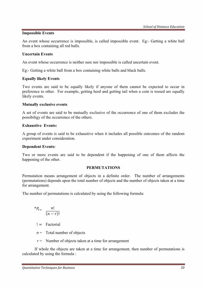
PERMUTATIONS
Permutation means arrangement of objects in a definite order. The number of arrangements (permutations) depends upon the total number of objects and the number of objects taken at a time for arrangement.
The number of permutations is calculated by using the following formula:
!!
! Factorial
n = Total number of objects
r = Number of objects taken at a time for arrangement
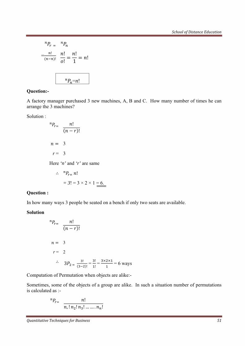
If whole the objects are taken at a time for arrangement, then number of permutations is calculated by using the formula :
School of Distance Education
Quantitative Techniques for Business 51
= !! !
!!1 !
=n!
Question:-
A factory manager purchased 3 new machines, A, B and C. How many number of times he can arrange the 3 machines?
Solution :
!!
3
r = 3
Here ‘n’ and ‘r’ are same
!
= 3! = 3 × 2 × 1 = 6.
Question :
In how many ways 3 people be seated on a bench if only two seats are available.
Solution
!!
3
r = 2
3 !!
= !! = = 6 ways
Computation of Permutation when objects are alike:-
Sometimes, some of the objects of a group are alike. In such a situation number of permutations is calculated as :-
!, ! ! ! …… . !
School of Distance Education
Quantitative Techniques for Business 52
number of alike objects in first category
= number of alike objects in second category
If all items are alike, you know, they can be arranged in only one order
ie , !!
Question:
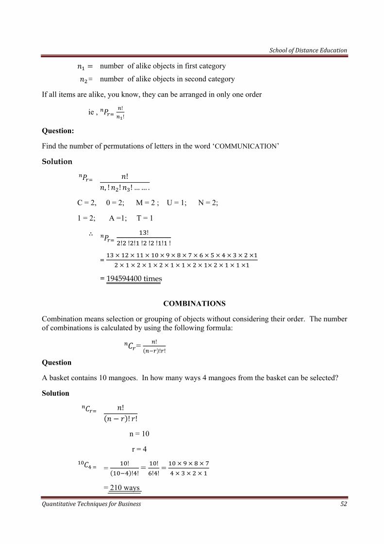
Find the number of permutations of letters in the word ‘COMMUNICATION’
Solution
!, ! ! ! …… .
C = 2, 0 = 2; M = 2 ; U = 1; N = 2;
1 = 2; A =1; T = 1
!! ! ! ! ! ! ! !
=
= 194594400 times
COMBINATIONS
Combination means selection or grouping of objects without considering their order. The number of combinations is calculated by using the following formula:
= !! !
Question
A basket contains 10 mangoes. In how many ways 4 mangoes from the basket can be selected?
Solution
!! !
n = 10
r = 4
= !! ! = !
! ! =
= 210 ways
School of Distance Education
Quantitative Techniques for Business 53
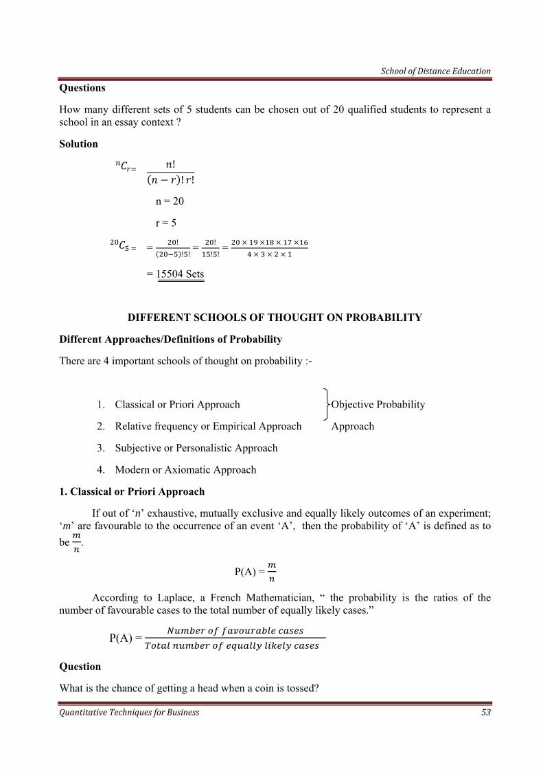
Questions
How many different sets of 5 students can be chosen out of 20 qualified students to represent a school in an essay context ?
Solution
!! !
n = 20
r = 5
= !! ! = !
! ! =
= 15504 Sets
DIFFERENT SCHOOLS OF THOUGHT ON PROBABILITY
Different Approaches/Definitions of Probability
There are 4 important schools of thought on probability :-
1. Classical or Priori Approach Objective Probability
2. Relative frequency or Empirical Approach Approach
3. Subjective or Personalistic Approach
4. Modern or Axiomatic Approach
1. Classical or Priori Approach
If out of ‘n’ exhaustive, mutually exclusive and equally likely outcomes of an experiment; ‘m’ are favourable to the occurrence of an event ‘A’, then the probability of ‘A’ is defined as to be .
P(A) =
According to Laplace, a French Mathematician, “ the probability is the ratios of the number of favourable cases to the total number of equally likely cases.”
P(A) =
Question
What is the chance of getting a head when a coin is tossed?
School of Distance Education
Quantitative Techniques for Business 54
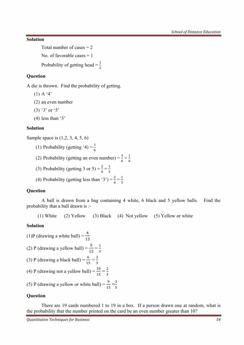
Solution Total number of cases = 2
No. of favorable cases = 1
Probability of getting head =
Question
A die is thrown. Find the probability of getting.
(1) A ‘4’
(2) an even number
(3) ‘3’ or ‘5’
(4) less than ‘3’
Solution
Sample space is (1,2, 3, 4, 5, 6)
(1) Probability (getting ‘4) =
(2) Probability (getting an even number) = =
(3) Probability (getting 3 or 5) = =
(4) Probability (getting less than ‘3’) = =
Question
A ball is drawn from a bag containing 4 white, 6 black and 5 yellow balls. Find the probability that a ball drawn is :-
(1) White (2) Yellow (3) Black (4) Not yellow (5) Yellow or white
Solution
(1)P (drawing a white ball) =
(2) P (drawing a yellow ball) = =
(3) P (drawing a black ball) = =
(4) P (drawing not a yellow ball) = =
(5) P (drawing a yellow or white ball) = =
Question
There are 19 cards numbered 1 to 19 in a box. If a person drawn one at random, what is the probability that the number printed on the card be an even number greater than 10?
School of Distance Education
Quantitative Techniques for Business 55
Solution
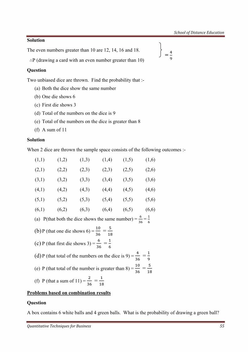
The even numbers greater than 10 are 12, 14, 16 and 18. =
P (drawing a card with an even number greater than 10)
Question
Two unbiased dice are thrown. Find the probability that :-
(a) Both the dice show the same number
(b) One die shows 6
(c) First die shows 3
(d) Total of the numbers on the dice is 9
(e) Total of the numbers on the dice is greater than 8
(f) A sum of 11
Solution
When 2 dice are thrown the sample space consists of the following outcomes :-
(1,1) (1,2) (1,3) (1,4) (1,5) (1,6)
(2,1) (2,2) (2,3) (2,3) (2,5) (2,6)
(3,1) (3,2) (3,3) (3,4) (3,5) (3,6)
(4,1) (4,2) (4,3) (4,4) (4,5) (4,6)
(5,1) (5,2) (5,3) (5,4) (5,5) (5,6)
(6,1) (6,2) (6,3) (6,4) (6,5) (6,6)
(a) P(that both the dice shows the same number) = =
(b) P (that one die shows 6) = =
(c) P (that first die shows 3) = =
(d) P (that total of the numbers on the dice is 9) = =
(e) P (that total of the number is greater than 8) = =
(f) P (that a sum of 11) = =
Problems based on combination results
Question
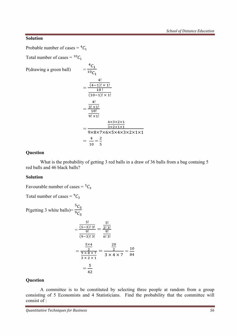
A box contains 6 white balls and 4 green balls. What is the probability of drawing a green ball?
School of Distance Education
Quantitative Techniques for Business 56
Solution
Probable number of cases =
Total number of cases =
P(drawing a green ball) =
= !! ! !! !
= !
! !!
! !
=
= =
Question
What is the probability of getting 3 red balls in a draw of 36 balls from a bag containg 5 red balls and 46 black balls?
Solution
Favourable number of cases =
Total number of cases =
P(getting 3 white balls)=
=
!! !!! !
= !! !!! !
=
=
=
=
Question
A committee is to be constituted by selecting three people at random from a group consisting of 5 Economists and 4 Statisticians. Find the probability that the committee will consist of :
School of Distance Education
Quantitative Techniques for Business 57
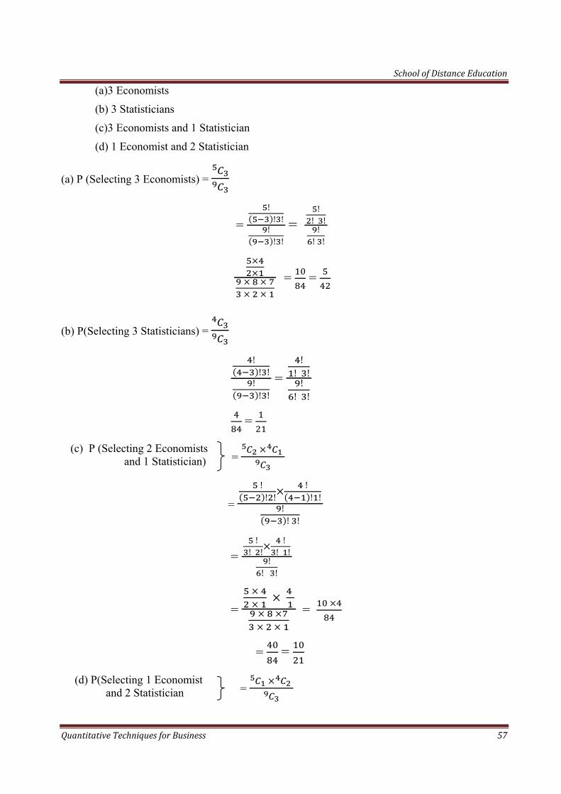
(a)3 Economists
(b) 3 Statisticians
(c)3 Economists and 1 Statistician
(d) 1 Economist and 2 Statistician
(a) P (Selecting 3 Economists) =
= !! !
!! ! =
!! !!! !
= =
(b) P(Selecting 3 Statisticians) =
!! !
!! !
= !
! !!
! !
=
(c) P (Selecting 2 Economists = and 1 Statistician)
=
!! !
!! !
!! !
= !! !
!! !
!! !
=
=
= =
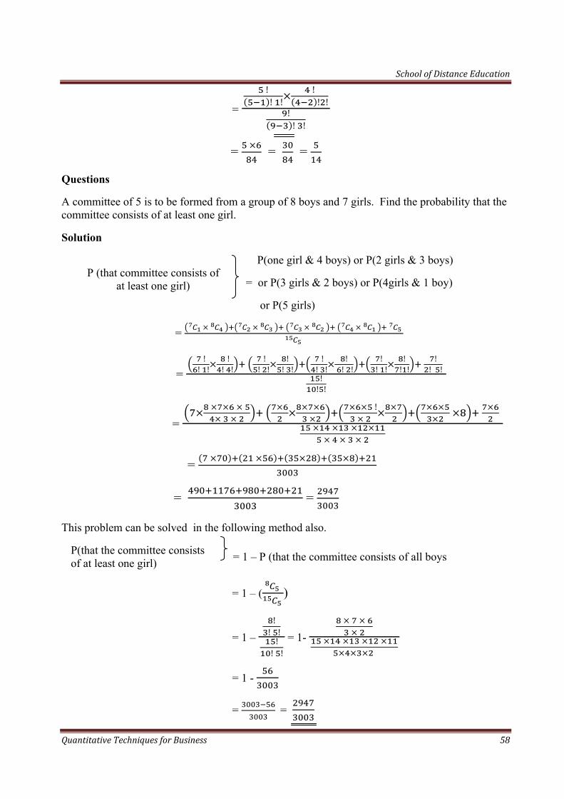
(d) P(Selecting 1 Economist = and 2 Statistician
School of Distance Education
Quantitative Techniques for Business 58
= !! !
!! !
!! !
= = =
Questions
A committee of 5 is to be formed from a group of 8 boys and 7 girls. Find the probability that the committee consists of at least one girl.
Solution
P (that committee consists of at least one girl)
P(one girl & 4 boys) or P(2 girls & 3 boys)
= or P(3 girls & 2 boys) or P(4girls & 1 boy)
or P(5 girls)
=
= !! !
!! ! !
! !!! !
!! !
! ! !
!! !
!! ! !
! ! !! !
=
!
=
= =
This problem can be solved in the following method also.
P(that the committee consists of at least one girl) = 1 – P (that the committee consists of all boys
= 1 – (
)
= 1 – !! !!! !
= 1-
= 1 -
= =
School of Distance Education
Quantitative Techniques for Business 59
Limitations of Classical Definition:
1. Classical definition has only limited application in coin-tossing die throwing etc. It fails to answer question like “What is the probability that a female will die before the age of 64?”
2. Classical definition cannot be applied when the possible outcomes are not equally likely. How can we apply classical definition to find the probability of rains? Here, two possibilities are “rain” or “no rain”. But at any given time these two possibilities are not equally likely.
3. Classical definition does not consider the outcomes of actual experimentations.
Relative Frequency Definition or Empirical Approach
According to Relative Frequency definition, the probability of an event can be defined as the relative frequency with which it occurs in an indefinitely large number of trials.
If an even ‘A’ occurs ‘f’ number of trials when a random experiment is repeated for ‘n’ number of
times, then P(A) =
For practical convenience, the above equation may be written as P(A) =
Here, probability has between 0 and 1,
i.e. 0 ≤ P(A) ≤ 1
Question
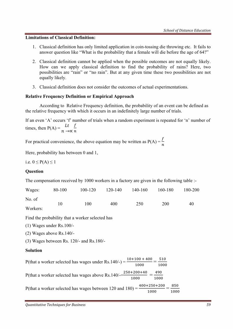
The compensation received by 1000 workers in a factory are given in the following table :-
Wages: 80-100 100-120 120-140 140-160 160-180 180-200
No. of
Workers: 10 100 400 250 200 40
Find the probability that a worker selected has
(1) Wages under Rs.100/-
(2) Wages above Rs.140/-
(3) Wages between Rs. 120/- and Rs.180/-
Solution
P(that a worker selected has wages under Rs.140/-) = =
P(that a worker selected has wages above Rs.140/-= =
P(that a worker selected has wages between 120 and 180) = =
School of Distance Education
Quantitative Techniques for Business 60
Subjective (Personalistie) Approach to Probability
The exponents of personalistie approach defines probability as a measure of personal confidence or belief based on whatever evidence is available. For example, if a teacher wants to find out the probability that Mr. X topping in M.Com examination, he may assign a value between zero and one according to his degree of belief for possible occurrence. He may take into account such factors as the past academic performance in terminal examinations etc. and arrive at a probability figure. The probability figure arrived under this method may vary from person to person. Hence it is called subjective method of probability.
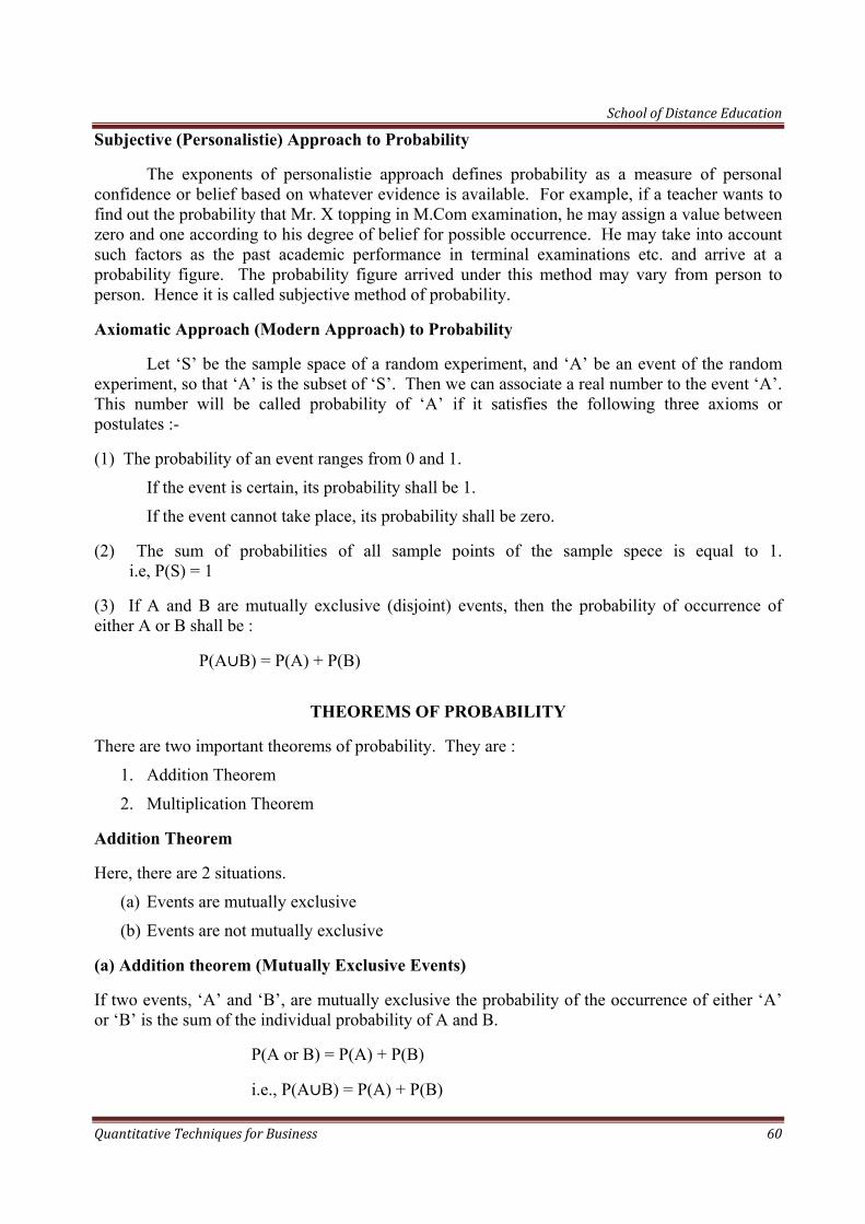
Axiomatic Approach (Modern Approach) to Probability
Let ‘S’ be the sample space of a random experiment, and ‘A’ be an event of the random experiment, so that ‘A’ is the subset of ‘S’. Then we can associate a real number to the event ‘A’. This number will be called probability of ‘A’ if it satisfies the following three axioms or postulates :-
(1) The probability of an event ranges from 0 and 1.
If the event is certain, its probability shall be 1.
If the event cannot take place, its probability shall be zero.
(2) The sum of probabilities of all sample points of the sample spece is equal to 1. i.e, P(S) = 1
(3) If A and B are mutually exclusive (disjoint) events, then the probability of occurrence of either A or B shall be :
P(A B) = P(A) + P(B)
THEOREMS OF PROBABILITY
There are two important theorems of probability. They are :
1. Addition Theorem
2. Multiplication Theorem
Addition Theorem
Here, there are 2 situations.
(a) Events are mutually exclusive
(b) Events are not mutually exclusive
(a) Addition theorem (Mutually Exclusive Events)
If two events, ‘A’ and ‘B’, are mutually exclusive the probability of the occurrence of either ‘A’ or ‘B’ is the sum of the individual probability of A and B.
P(A or B) = P(A) + P(B)
i.e., P(A B) = P(A) + P(B)

School of Distance Education
Quantitative Techniques for Business 61
(b)Addition theorem (Not mutually exclusive events)
If two events, A and B are not mutually exclusive the probability of the occurrence of either A or B is the sum of their individual probability minus probability for both to happen.
P(A or B) = P(A) + P(B) – P(A and B)
i.e., P(A B) = P(A) + P(B) – P(A∩B)
Question
What is the probability of picking a card that was red or black?
Solution
Here the events are mutually exclusive
P(picking a red card) =
P(picking a black card) =
P (picking a red or black card) = + = 1
Question
The probability that a contractor will get a plumping contract is and the probability that
he will not get an electric contract is . If the probability of getting at least one contract is , what is the probability that he will get both the contracts?
Solution
P(getting plumbing contract) =
P(not getting electric contract) =
P(getting electric contract) = 1 - =
P(getting at least one contract) = P (getting electric contract) +
P(getting plumbing contract) - P(getting both)
i.e., = + - P(getting both)
P(getting both contracts) = + -
= =
School of Distance Education
Quantitative Techniques for Business 62
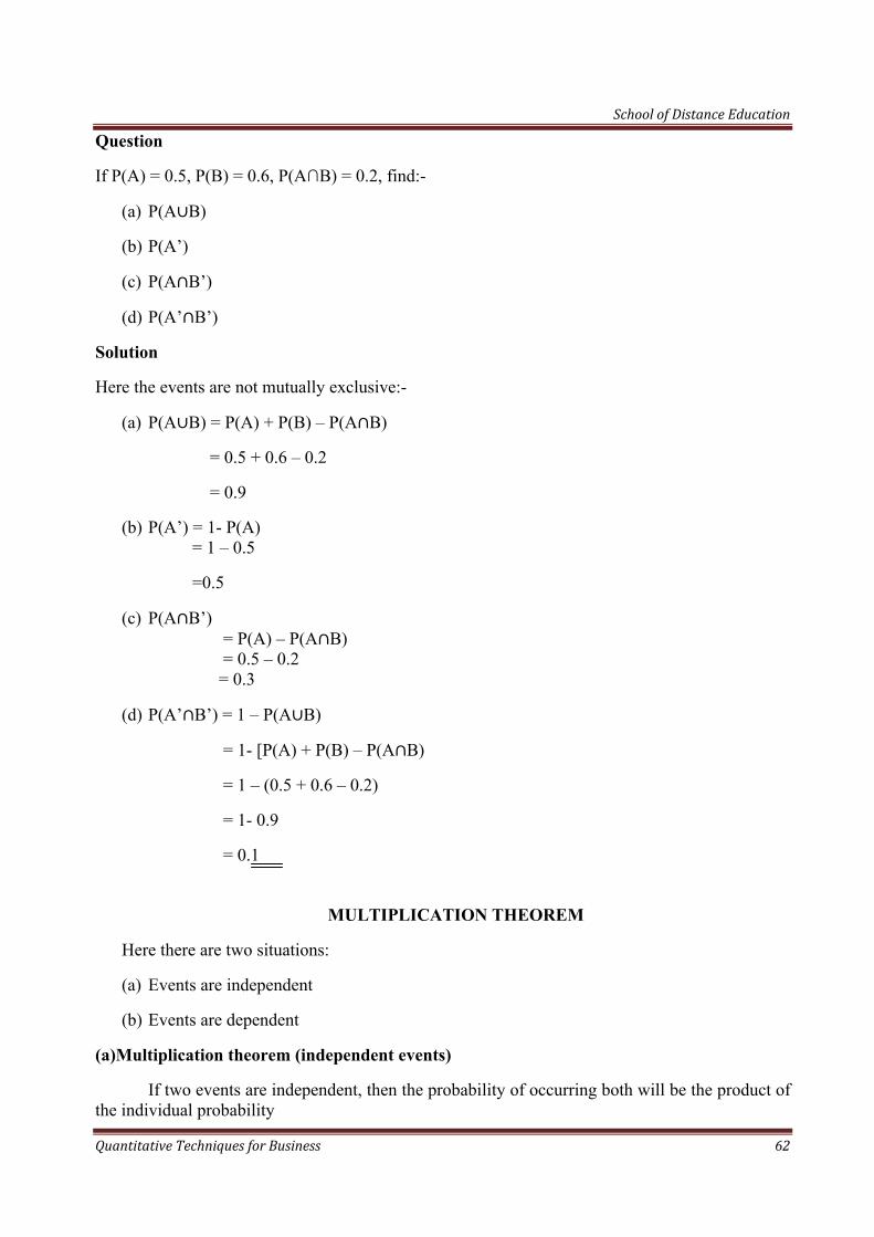
Question
If P(A) = 0.5, P(B) = 0.6, P(A∩B) = 0.2, find:-
(a) P(A B)
(b) P(A’)
(c) P(A B’)
(d) P(A’ B’)
Solution
Here the events are not mutually exclusive:-
(a) P(A B) = P(A) + P(B) – P(A B)
= 0.5 + 0.6 – 0.2
= 0.9
(b) P(A’) = 1- P(A) = 1 – 0.5
=0.5
(c) P(A B’) = P(A) – P(A B) = 0.5 – 0.2 = 0.3
(d) P(A’ B’) = 1 – P(A B)
= 1- [P(A) + P(B) – P(A B)
= 1 – (0.5 + 0.6 – 0.2)
= 1- 0.9
= 0.1
MULTIPLICATION THEOREM
Here there are two situations:
(a) Events are independent
(b) Events are dependent
(a)Multiplication theorem (independent events)
If two events are independent, then the probability of occurring both will be the product of the individual probability
School of Distance Education
Quantitative Techniques for Business 63
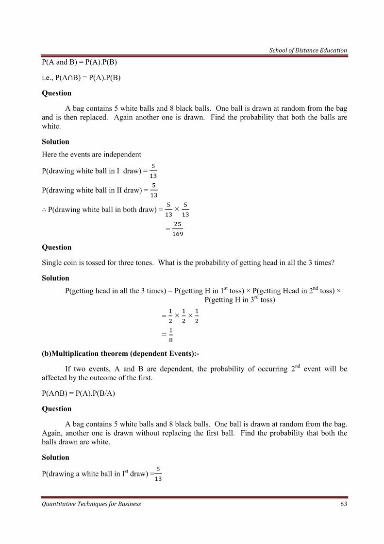
P(A and B) = P(A).P(B)
i.e., P(A B) = P(A).P(B)
Question
A bag contains 5 white balls and 8 black balls. One ball is drawn at random from the bag and is then replaced. Again another one is drawn. Find the probability that both the balls are white.
Solution Here the events are independent
P(drawing white ball in I draw) =
P(drawing white ball in II draw) =
P(drawing white ball in both draw) = ×
=
Question
Single coin is tossed for three tones. What is the probability of getting head in all the 3 times?
Solution P(getting head in all the 3 times) = P(getting H in 1st toss) × P(getting Head in 2nd toss) × P(getting H in 3rd toss)
= × ×
=
(b)Multiplication theorem (dependent Events):-
If two events, A and B are dependent, the probability of occurring 2nd event will be affected by the outcome of the first.
P(A B) = P(A).P(B/A)
Question
A bag contains 5 white balls and 8 black balls. One ball is drawn at random from the bag. Again, another one is drawn without replacing the first ball. Find the probability that both the balls drawn are white.
Solution
P(drawing a white ball in Ist draw) =

School of Distance Education
Quantitative Techniques for Business 64
P (drawing a white ball in IInd draw) =
=
Question
The probability that ‘A’ solves a problem in Maths is and the probability that ‘B’ solves it is . If they try independently find the probability that :-
(i) Both solve the problem.
(ii) at least one solve the problem.
(iii) none solve the problem.
Solution
(i) P(that both solve the problem) = P(that A solves the problem)× P(that B solves the problem)
= × = =
(ii) P(that at least one = P(that A or B solves the problem) solve the problem) = P(A solve the problem + P(B solve the problem – P(A and B solve the problem)
= + - ( × )
= + -
=
= =
(iii) P(that none solve the problem) =1-P(at least one solve the problem)
= 1 – P(A or B solve the problem)
=1- [P(A solve the problem +
P(B solve the problem) -
P(A & B solve the problem)]
= 1-
= 1-( )
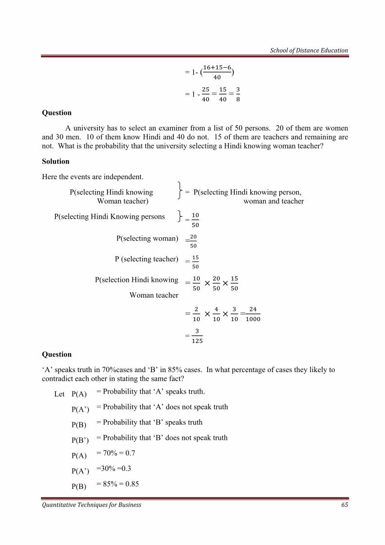
School of Distance Education
Quantitative Techniques for Business 65
= 1- ( )
= 1 - = =
Question
A university has to select an examiner from a list of 50 persons. 20 of them are women and 30 men. 10 of them know Hindi and 40 do not. 15 of them are teachers and remaining are not. What is the probability that the university selecting a Hindi knowing woman teacher?
Solution
Here the events are independent.
P(selecting Hindi knowing Woman teacher)
= P(selecting Hindi knowing person, woman and teacher
P(selecting Hindi Knowing persons =
P(selecting woman) =
P (selecting teacher) =
P(selection Hindi knowing
Woman teacher=
= =
=
Question
‘A’ speaks truth in 70%cases and ‘B’ in 85% cases. In what percentage of cases they likely to contradict each other in stating the same fact?
Let P(A) = Probability that ‘A’ speaks truth.
P(A’) = Probability that ‘A’ does not speak truth
P(B) = Probability that ‘B’ speaks truth
P(B’) = Probability that ‘B’ does not speak truth
P(A) = 70% = 0.7
P(A’) =30% =0.3
P(B) = 85% = 0.85
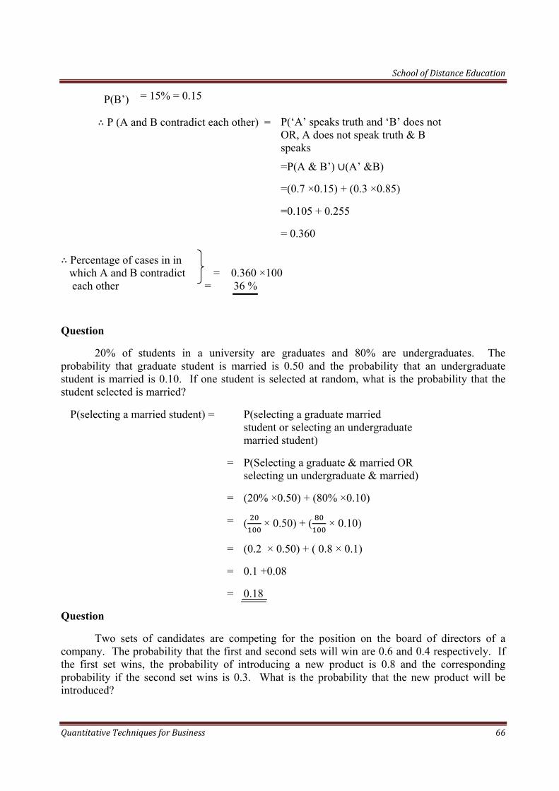
School of Distance Education
Quantitative Techniques for Business 66
P(B’) = 15% = 0.15
P (A and B contradict each other) = P(‘A’ speaks truth and ‘B’ does not OR, A does not speak truth & B speaks
=P(A & B’) (A’ &B)
=(0.7 ×0.15) + (0.3 ×0.85)
=0.105 + 0.255
= 0.360
Percentage of cases in in which A and B contradict = 0.360 ×100 each other = 36 %
Question
20% of students in a university are graduates and 80% are undergraduates. The probability that graduate student is married is 0.50 and the probability that an undergraduate student is married is 0.10. If one student is selected at random, what is the probability that the student selected is married?
P(selecting a married student) = P(selecting a graduate married student or selecting an undergraduate married student)
= P(Selecting a graduate & married OR selecting un undergraduate & married)
= (20% ×0.50) + (80% ×0.10)
= ( × 0.50) + ( × 0.10)
= (0.2 × 0.50) + ( 0.8 × 0.1)
= 0.1 +0.08
= 0.18
Question
Two sets of candidates are competing for the position on the board of directors of a company. The probability that the first and second sets will win are 0.6 and 0.4 respectively. If the first set wins, the probability of introducing a new product is 0.8 and the corresponding probability if the second set wins is 0.3. What is the probability that the new product will be introduced?

School of Distance Education
Quantitative Techniques for Business 67
Solution
P(that new product will be introduced) =
P(that new product is introduced by first set OR the new product is introduced by second set)
= P (Ist set wins & Ist introduced the new produced OR IInd set wins the new product)
= (0.6 × 0.8) + (0.4 × 0.3)
= 0.48 + 0.12
= 0.60
Question
A certain player say Mr. X is known to win with possibility 0.3 if the truck is fast and 0.4 if the track is slow. For Monday there is a 0.7 probability of a fast track and 0.3 probability of a slow track. What is the probability that Mr. X will win on Monday?
Solution
P(X will won on Monday) = P(to win in fast track OR to win in slow track)
= P (to get fast track & to win
to get slow track & to win) OR
= (0.7 × 0.3) + (0. 3 × 0. 4)
= 0.21 + 0.12
= 0.33
CONDITIONAL PROBABILITY
Multiplication theorem states that if two events, A and B, are dependent events then, the probability of happening both will be the product of P(A) and P(B/A).
i.e., P(A and B) or = P(A).P(B/A)
P(A B )
Here, P (B/A) is called Conditional probability
P(A B) = P(A).P( )
i.e., P(A).P( ) = P(A B)
P( ) = P A BP A
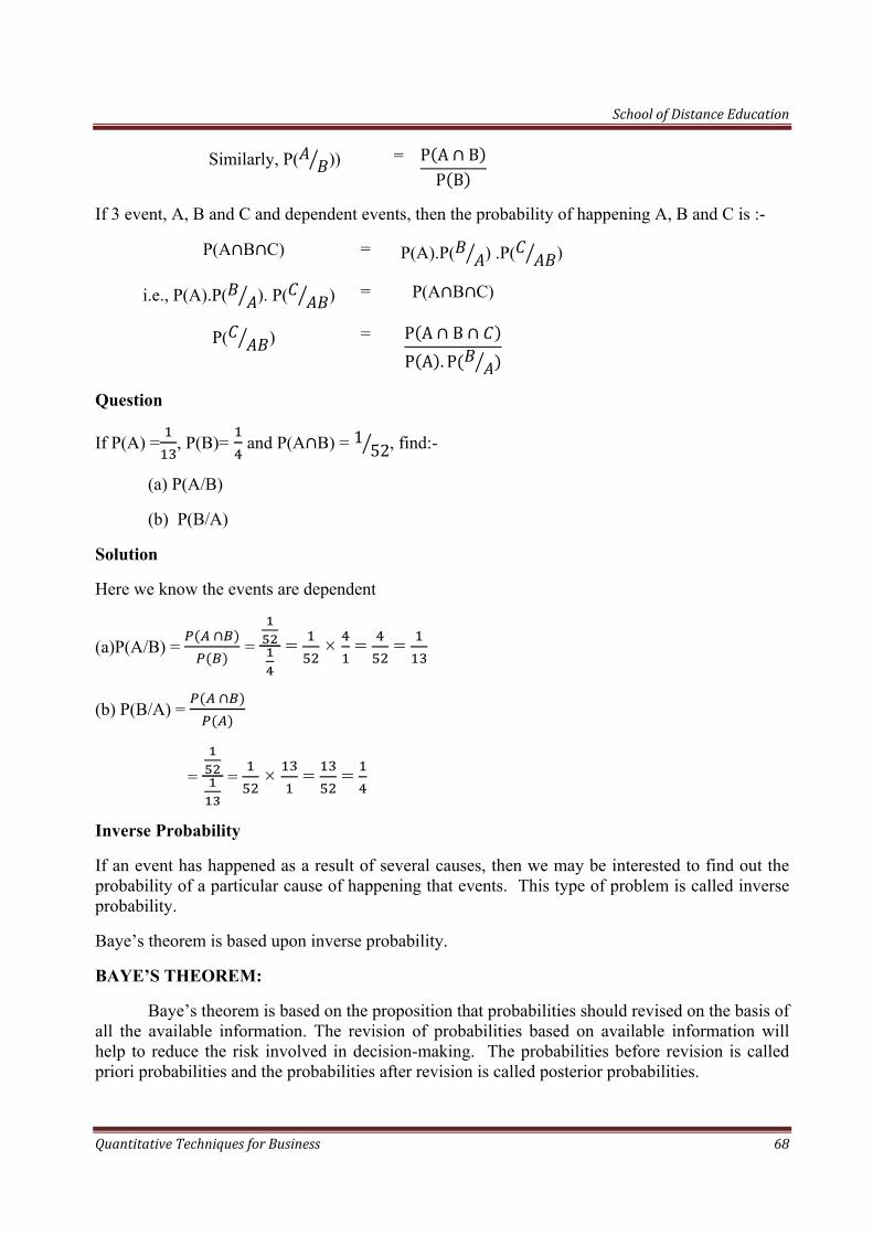
School of Distance Education
Quantitative Techniques for Business 68
Similarly, P( )) = P A BP B
If 3 event, A, B and C and dependent events, then the probability of happening A, B and C is :-
P(A B C) = P(A).P( ) .P( )
i.e., P(A).P( ). P( ) = P(A B C)
P( ) = P A BP A . P
Question
If P(A) = , P(B)= and P(A B) = 1 52, find:-
(a) P(A/B)
(b) P(B/A)
Solution
Here we know the events are dependent
(a)P(A/B) = = = × = =
(b) P(B/A) =
= = × = =
Inverse Probability
If an event has happened as a result of several causes, then we may be interested to find out the probability of a particular cause of happening that events. This type of problem is called inverse probability.
Baye’s theorem is based upon inverse probability.
BAYE’S THEOREM:
Baye’s theorem is based on the proposition that probabilities should revised on the basis of all the available information. The revision of probabilities based on available information will help to reduce the risk involved in decision-making. The probabilities before revision is called priori probabilities and the probabilities after revision is called posterior probabilities.
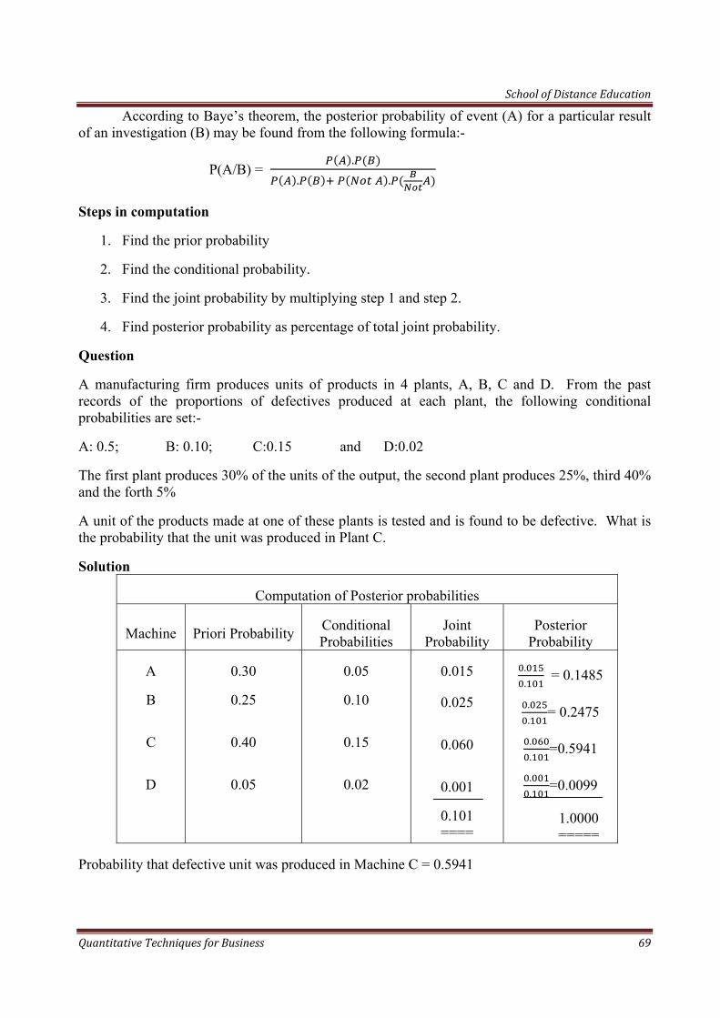
School of Distance Education
Quantitative Techniques for Business 69
According to Baye’s theorem, the posterior probability of event (A) for a particular result of an investigation (B) may be found from the following formula:-
P(A/B) = .
. .
Steps in computation
1. Find the prior probability
2. Find the conditional probability.
3. Find the joint probability by multiplying step 1 and step 2.
4. Find posterior probability as percentage of total joint probability.
Question
A manufacturing firm produces units of products in 4 plants, A, B, C and D. From the past records of the proportions of defectives produced at each plant, the following conditional probabilities are set:-
A: 0.5; B: 0.10; C:0.15 and D:0.02
The first plant produces 30% of the units of the output, the second plant produces 25%, third 40% and the forth 5%
A unit of the products made at one of these plants is tested and is found to be defective. What is the probability that the unit was produced in Plant C.
Solution
Computation of Posterior probabilities
Machine Priori Probability Conditional Probabilities
Joint Probability
Posterior Probability
A
B
C
D
0.30
0.25
0.40
0.05
0.05
0.10
0.15
0.02
0.015
0.025
0.060
0.001
0.101 ====
.
. = 0.1485
.
.= 0.2475
.
.=0.5941
.
.=0.0099
1.0000 =====
Probability that defective unit was produced in Machine C = 0.5941
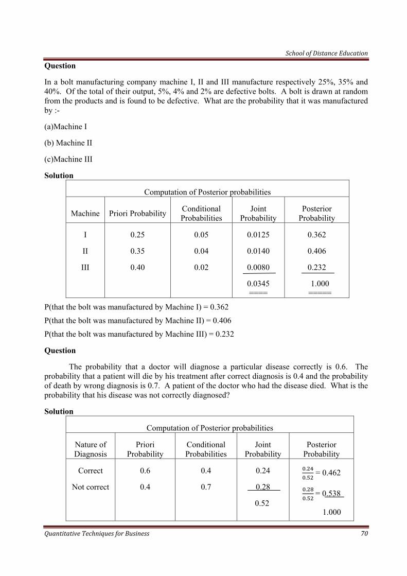
School of Distance Education
Quantitative Techniques for Business 70
Question
In a bolt manufacturing company machine I, II and III manufacture respectively 25%, 35% and 40%. Of the total of their output, 5%, 4% and 2% are defective bolts. A bolt is drawn at random from the products and is found to be defective. What are the probability that it was manufactured by :-
(a)Machine I
(b) Machine II
(c)Machine III
Solution
Computation of Posterior probabilities
Machine Priori Probability Conditional Probabilities
Joint Probability
Posterior Probability
I
II
III
0.25
0.35
0.40
0.05
0.04
0.02
0.0125
0.0140
0.0080
0.0345 ====
0.362
0.406
0.232
1.000 =====
P(that the bolt was manufactured by Machine I) = 0.362
P(that the bolt was manufactured by Machine II) = 0.406
P(that the bolt was manufactured by Machine III) = 0.232
Question
The probability that a doctor will diagnose a particular disease correctly is 0.6. The probability that a patient will die by his treatment after correct diagnosis is 0.4 and the probability of death by wrong diagnosis is 0.7. A patient of the doctor who had the disease died. What is the probability that his disease was not correctly diagnosed?
Solution
Computation of Posterior probabilities
Nature of Diagnosis
Priori Probability
Conditional Probabilities
Joint Probability
Posterior Probability
Correct
Not correct
0.6
0.4
0.4
0.7
0.24
0.28
0.52
.
. = 0.462
.
. = 0.538
1.000
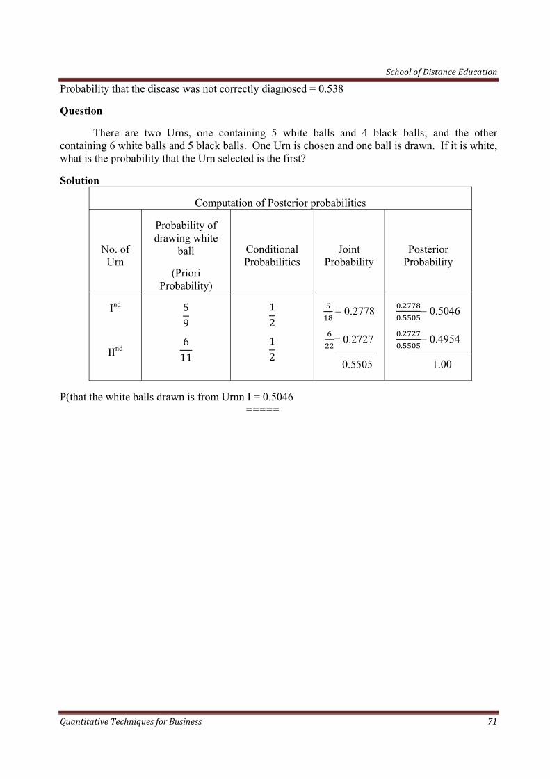
School of Distance Education
Quantitative Techniques for Business 71
Probability that the disease was not correctly diagnosed = 0.538
Question
There are two Urns, one containing 5 white balls and 4 black balls; and the other containing 6 white balls and 5 black balls. One Urn is chosen and one ball is drawn. If it is white, what is the probability that the Urn selected is the first?
Solution
Computation of Posterior probabilities
No. of Urn
Probability of drawing white
ball
(Priori Probability)
Conditional Probabilities
Joint Probability
Posterior Probability
Ind
IInd
59
611
12
12
= 0.2778
= 0.2727
0.5505
.
.= 0.5046
.
.= 0.4954
1.00
P(that the white balls drawn is from Urnn I = 0.5046 =====
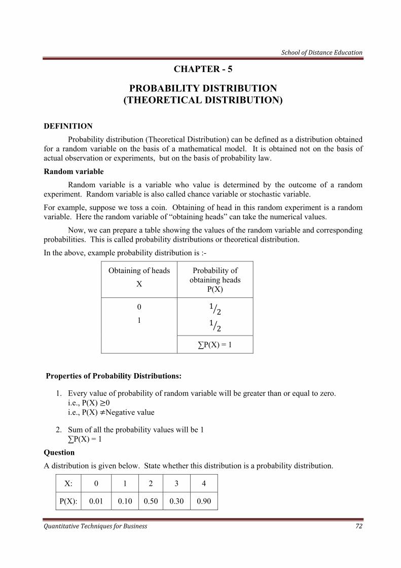
School of Distance Education
Quantitative Techniques for Business 72
CHAPTER - 5
PROBABILITY DISTRIBUTION (THEORETICAL DISTRIBUTION)
DEFINITION
Probability distribution (Theoretical Distribution) can be defined as a distribution obtained for a random variable on the basis of a mathematical model. It is obtained not on the basis of actual observation or experiments, but on the basis of probability law.
Random variable Random variable is a variable who value is determined by the outcome of a random
experiment. Random variable is also called chance variable or stochastic variable.
For example, suppose we toss a coin. Obtaining of head in this random experiment is a random variable. Here the random variable of “obtaining heads” can take the numerical values.
Now, we can prepare a table showing the values of the random variable and corresponding probabilities. This is called probability distributions or theoretical distribution.
In the above, example probability distribution is :-
Obtaining of heads
X
Probability of obtaining heads
P(X)
0
1
12
12
∑P(X) = 1
Properties of Probability Distributions:
1. Every value of probability of random variable will be greater than or equal to zero. i.e., P(X) 0 i.e., P(X) Negative value
2. Sum of all the probability values will be 1 ∑P(X) = 1
Question A distribution is given below. State whether this distribution is a probability distribution.
X: 0 1 2 3 4
P(X): 0.01 0.10 0.50 0.30 0.90
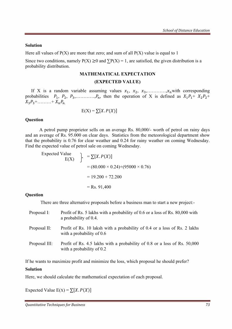
School of Distance Education
Quantitative Techniques for Business 73
Solution Here all values of P(X) are more that zero; and sum of all P(X) value is equal to 1
Since two conditions, namely P(X) 0 and ∑P(X) = 1, are satisfied, the given distribution is a probability distribution.
MATHEMATICAL EXPECTATION
(EXPECTED VALUE)
If X is a random variable assuming values , , ,…………, with corresponding probabilities , , ,…………, , then the operation of X is defined as + +
+………+ .
E(X) = ∑ .
Question
A petrol pump proprietor sells on an average Rs. 80,000/- worth of petrol on rainy days and an average of Rs. 95.000 on clear days. Statistics from the meteorological department show that the probability is 0.76 for clear weather and 0.24 for rainy weather on coming Wednesday. Find the expected value of petrol sale on coming Wednesday.
Expected Value = ∑ . E(X) = (80.000 × 0.24)+(95000 × 0.76)
= 19.200 + 72.200
= Rs. 91,400
Question There are three alternative proposals before a business man to start a new project:-
Proposal I: Profit of Rs. 5 lakhs with a probability of 0.6 or a loss of Rs. 80,000 with a probability of 0.4.
Proposal II: Profit of Rs. 10 laksh with a probability of 0.4 or a loss of Rs. 2 lakhs with a probability of 0.6
Proposal III: Profit of Rs. 4.5 lakhs with a probability of 0.8 or a loss of Rs. 50,000 with a probability of 0.2
If he wants to maximize profit and minimize the loss, which proposal he should prefer?
Solution Here, we should calculate the mathematical expectation of each proposal.
Expected Value E(X) = ∑ .
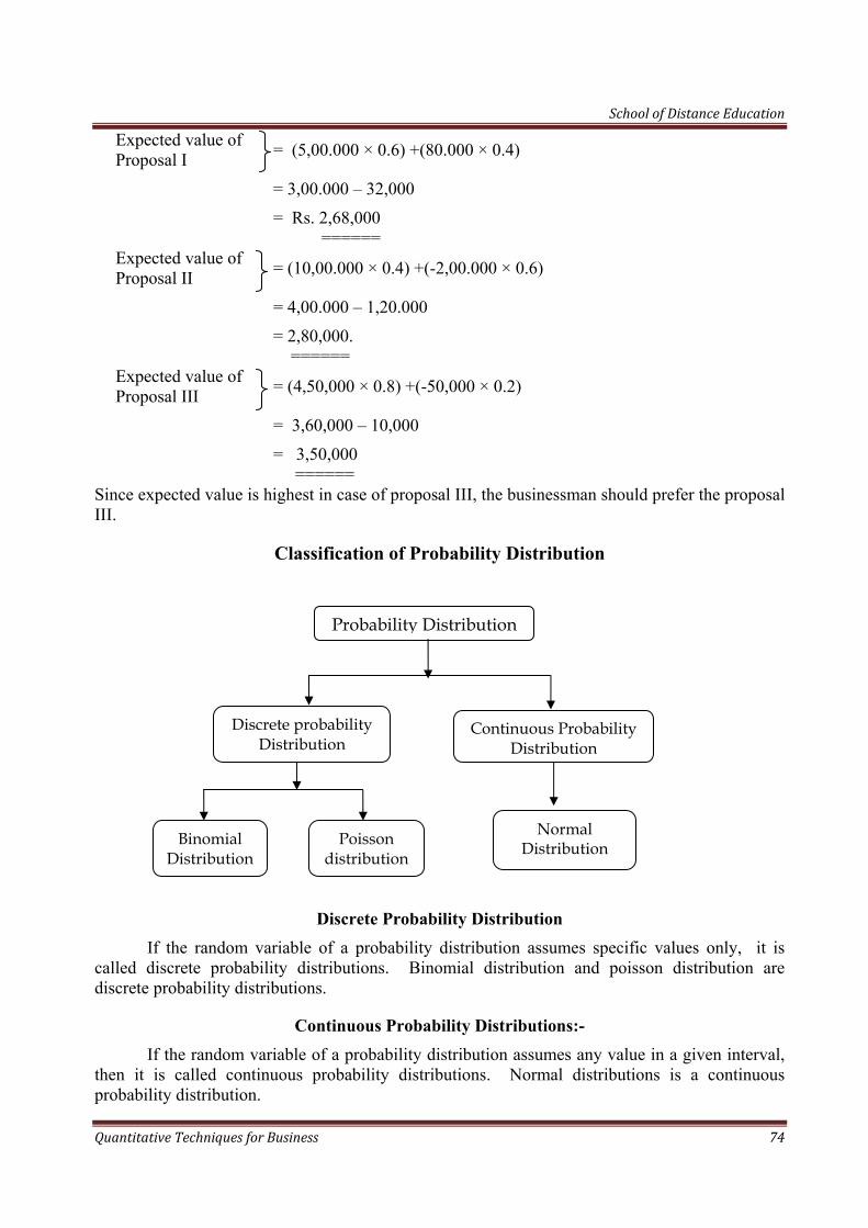
School of Distance Education
Quantitative Techniques for Business 74
Expected value of = (5,00.000 × 0.6) +(80.000 × 0.4) Proposal I = 3,00.000 – 32,000
= Rs. 2,68,000 ======
Expected value of = (10,00.000 × 0.4) +(-2,00.000 × 0.6) Proposal II
= 4,00.000 – 1,20.000
= 2,80,000. ======
Expected value of = (4,50,000 × 0.8) +(-50,000 × 0.2) Proposal III
= 3,60,000 – 10,000
= 3,50,000 ======
Since expected value is highest in case of proposal III, the businessman should prefer the proposal III.
Classification of Probability Distribution
Discrete Probability Distribution If the random variable of a probability distribution assumes specific values only, it is
called discrete probability distributions. Binomial distribution and poisson distribution are discrete probability distributions.
Continuous Probability Distributions:- If the random variable of a probability distribution assumes any value in a given interval,
then it is called continuous probability distributions. Normal distributions is a continuous probability distribution.
Discrete probability Distribution
Continuous Probability Distribution
Probability Distribution
Binomial Distribution
Poisson distribution
Normal Distribution
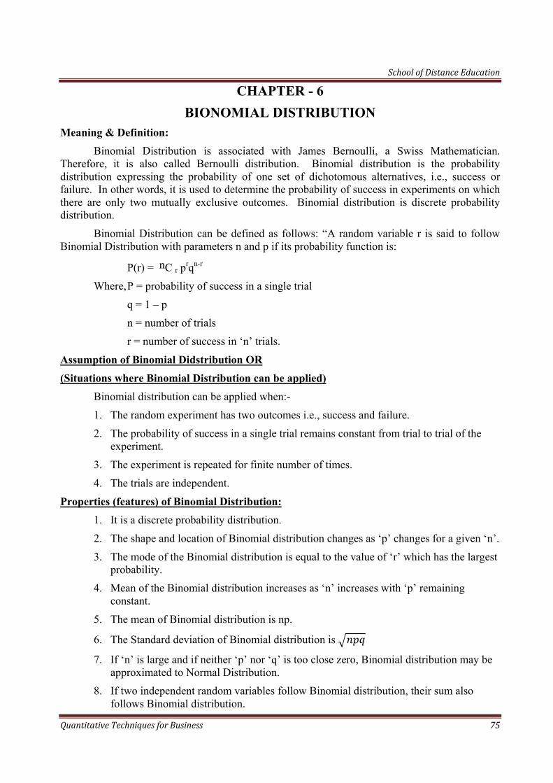
School of Distance Education
Quantitative Techniques for Business 75
CHAPTER - 6 BIONOMIAL DISTRIBUTION
Meaning & Definition: Binomial Distribution is associated with James Bernoulli, a Swiss Mathematician. Therefore, it is also called Bernoulli distribution. Binomial distribution is the probability distribution expressing the probability of one set of dichotomous alternatives, i.e., success or failure. In other words, it is used to determine the probability of success in experiments on which there are only two mutually exclusive outcomes. Binomial distribution is discrete probability distribution.
Binomial Distribution can be defined as follows: “A random variable r is said to follow Binomial Distribution with parameters n and p if its probability function is:
P(r) = nC r prqn-r
Where, P = probability of success in a single trial
q = 1 – p
n = number of trials
r = number of success in ‘n’ trials.
Assumption of Binomial Didstribution OR
(Situations where Binomial Distribution can be applied) Binomial distribution can be applied when:-
1. The random experiment has two outcomes i.e., success and failure.
2. The probability of success in a single trial remains constant from trial to trial of the experiment.
3. The experiment is repeated for finite number of times.
4. The trials are independent.
Properties (features) of Binomial Distribution: 1. It is a discrete probability distribution.
2. The shape and location of Binomial distribution changes as ‘p’ changes for a given ‘n’.
3. The mode of the Binomial distribution is equal to the value of ‘r’ which has the largest probability.
4. Mean of the Binomial distribution increases as ‘n’ increases with ‘p’ remaining constant.
5. The mean of Binomial distribution is np.
6. The Standard deviation of Binomial distribution is
7. If ‘n’ is large and if neither ‘p’ nor ‘q’ is too close zero, Binomial distribution may be approximated to Normal Distribution.
8. If two independent random variables follow Binomial distribution, their sum also follows Binomial distribution.
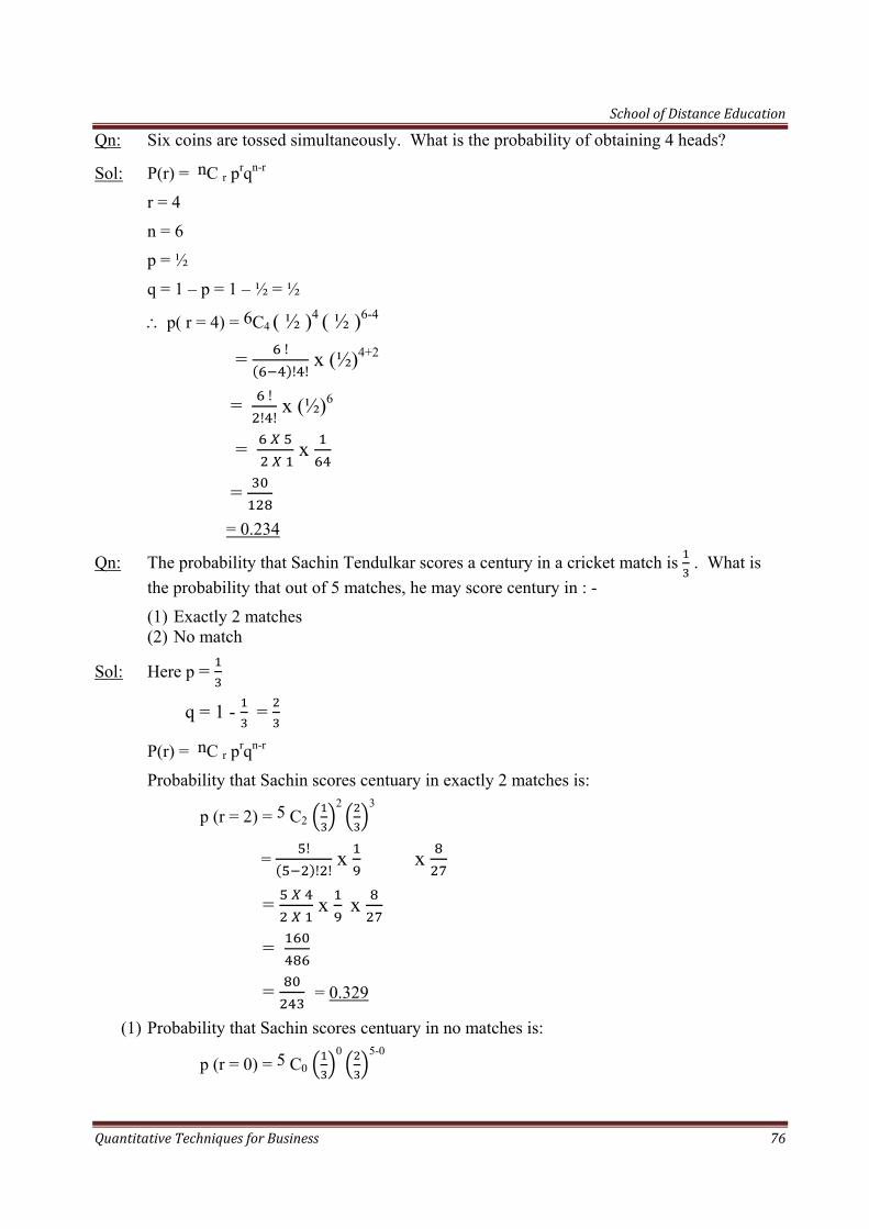
School of Distance Education
Quantitative Techniques for Business 76
Qn: Six coins are tossed simultaneously. What is the probability of obtaining 4 heads?
Sol: P(r) = nC r prqn-r r = 4
n = 6
p = ½
q = 1 – p = 1 – ½ = ½
∴ p( r = 4) = 6C4 ( ½ )4 ( ½ )6-4
= !! !
x (½)4+2
= !! !
x (½)6
=
x
=
= 0.234
Qn: The probability that Sachin Tendulkar scores a century in a cricket match is . What is the probability that out of 5 matches, he may score century in : -
(1) Exactly 2 matches (2) No match
Sol: Here p =
q = 1 - =
P(r) = nC r prqn-r
Probability that Sachin scores centuary in exactly 2 matches is:
p (r = 2) = 5 C2 2 3
= !! !
x x
=
x x
=
= = 0.329
(1) Probability that Sachin scores centuary in no matches is:
p (r = 0) = 5 C0 0 5-0
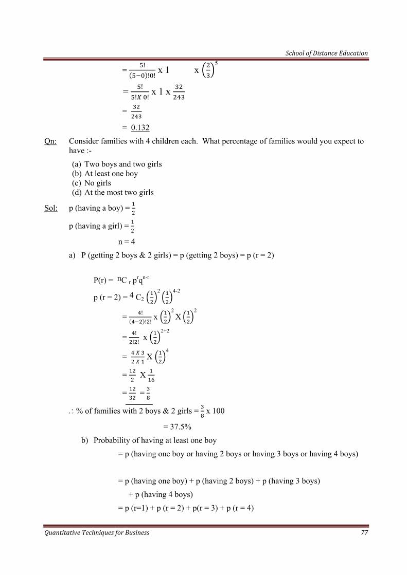
School of Distance Education
Quantitative Techniques for Business 77
= !! !
x 1 x 5
= !! !
x 1 x
=
= 0.132
Qn: Consider families with 4 children each. What percentage of families would you expect to have :-
(a) Two boys and two girls (b) At least one boy (c) No girls (d) At the most two girls
Sol: p (having a boy) =
p (having a girl) =
n = 4
a) P (getting 2 boys & 2 girls) = p (getting 2 boys) = p (r = 2)
P(r) = nC r prqn-r
p (r = 2) = 4 C2 2 4-2
= !! !
x 2 X 2
= !! !
x 2+2
=
X 4
= X
= =
∴% of families with 2 boys & 2 girls = x 100
= 37.5%
b) Probability of having at least one boy
= p (having one boy or having 2 boys or having 3 boys or having 4 boys)
= p (having one boy) + p (having 2 boys) + p (having 3 boys)
+ p (having 4 boys)
= p (r=1) + p (r = 2) + p(r = 3) + p (r = 4)
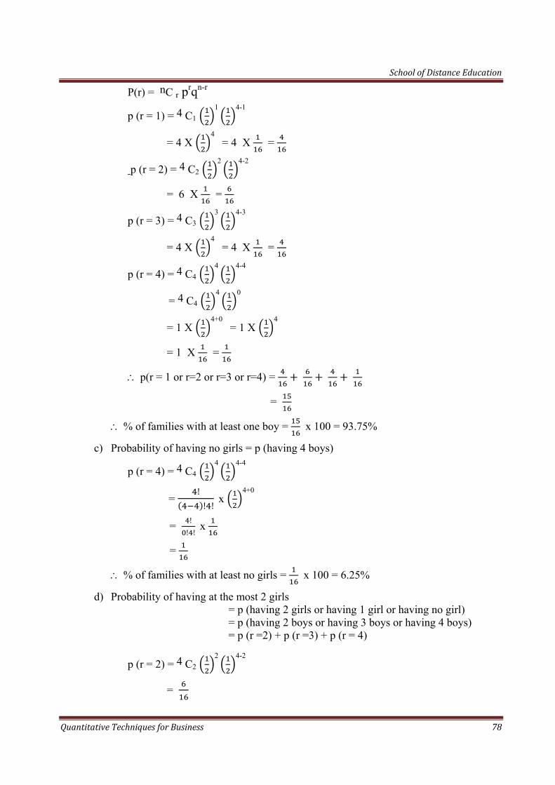
School of Distance Education
Quantitative Techniques for Business 78
P(r) = nC r prqn-r
p (r = 1) = 4 C1 1 4-1
= 4 X 4 = 4 X =
p (r = 2) = 4 C2 2 4-2
= 6 X =
p (r = 3) = 4 C3 3 4-3
= 4 X 4 = 4 X =
p (r = 4) = 4 C4 4 4-4
= 4 C4 4 0
= 1 X 4+0 = 1 X
4
= 1 X =
∴ p(r = 1 or r=2 or r=3 or r=4) =
=
∴ % of families with at least one boy = x 100 = 93.75%
c) Probability of having no girls = p (having 4 boys)
p (r = 4) = 4 C4 4 4-4
= !! !
x 4+0
= !! !
x
=
∴ % of families with at least no girls = x 100 = 6.25%
d) Probability of having at the most 2 girls = p (having 2 girls or having 1 girl or having no girl) = p (having 2 boys or having 3 boys or having 4 boys) = p (r =2) + p (r =3) + p (r = 4)
p (r = 2) = 4 C2 2 4-2
=
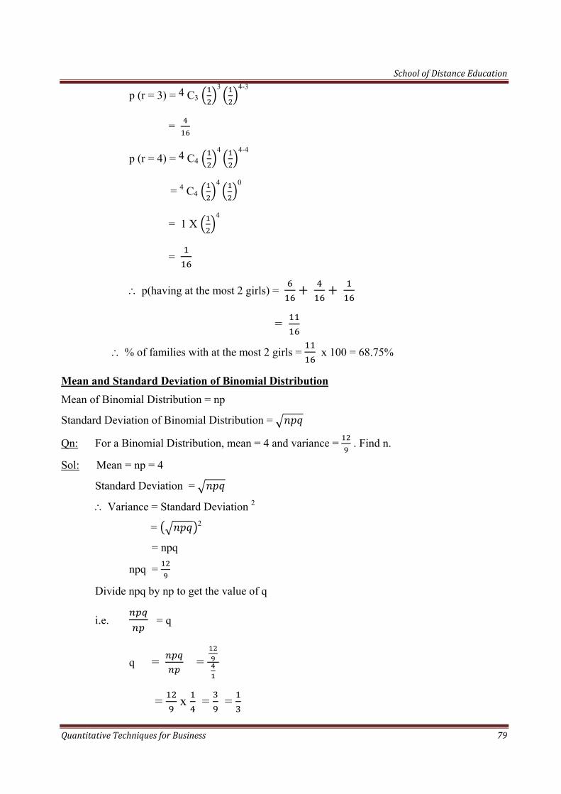
School of Distance Education
Quantitative Techniques for Business 79
p (r = 3) = 4 C3 3 4-3
=
p (r = 4) = 4 C4 4 4-4
= 4 C4 4 0
= 1 X 4
=
∴ p(having at the most 2 girls) =
=
∴ % of families with at the most 2 girls = x 100 = 68.75%
Mean and Standard Deviation of Binomial Distribution Mean of Binomial Distribution = np
Standard Deviation of Binomial Distribution =
Qn: For a Binomial Distribution, mean = 4 and variance = . Find n.
Sol: Mean = np = 4
Standard Deviation =
∴ Variance = Standard Deviation 2
= 2
= npq
npq =
Divide npq by np to get the value of q
i.e. = q
q = =
= x = =

School of Distance Education
Quantitative Techniques for Business 80
q =
p = 1 – q
= 1 - =
np = 4
n x = 4
n = 4
n = 4 x = 6
Qn: For a Binomial Distribution, mean is 6 and Standard Deviation is √2 . Find the parameters.
Sol: Mean (np) = 6
Standard Deviation ( ) = √2
∴ npq = 2
=
q =
∴ p = 1 – q
= 1 - =
np = 6
n x = 6
∴ n = = 6 x = 9
Value of parameters:
p = q = n = 9
Qn: In a Binomial Distribution consisting 5 independent trials, probability for 1 and 2 successes are 0.4096 and 0.2048 respectively. Find the parameter p.
Sol: As there are 5 trials, the terms of the Binomial Distribution are:-
p (r = 0) ; p (r = 1); p (r = 2); p (r = 3); p (r = 4) and p (r = 5)
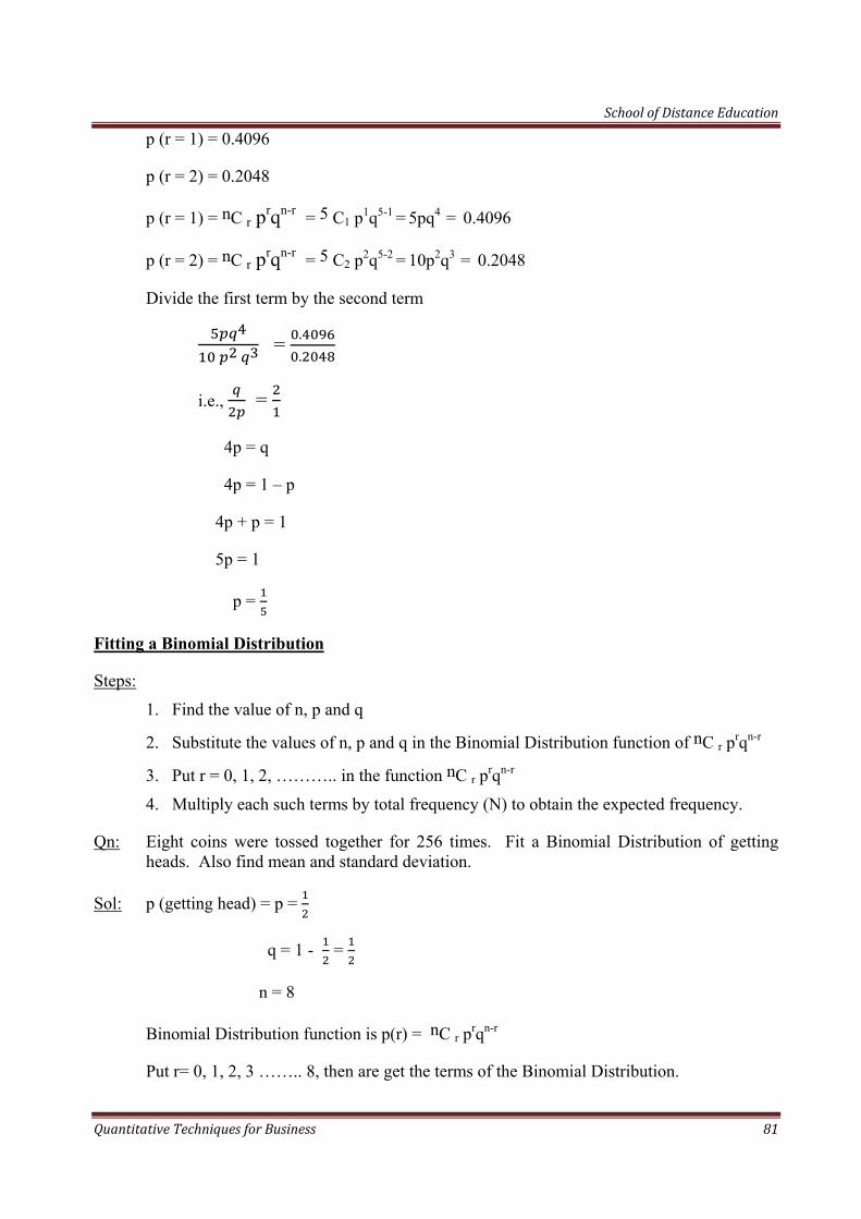
School of Distance Education
Quantitative Techniques for Business 81
p (r = 1) = 0.4096
p (r = 2) = 0.2048
p (r = 1) = nC r prqn-r = 5 C1 p1q5-1 = 5pq4 = 0.4096
p (r = 2) = nC r prqn-r = 5 C2 p2q5-2 = 10p2q3 = 0.2048
Divide the first term by the second term
= ..
i.e., =
4p = q
4p = 1 – p
4p + p = 1
5p = 1
p =
Fitting a Binomial Distribution
Steps:
1. Find the value of n, p and q
2. Substitute the values of n, p and q in the Binomial Distribution function of nC r prqn-r
3. Put r = 0, 1, 2, ……….. in the function nC r prqn-r
4. Multiply each such terms by total frequency (N) to obtain the expected frequency.
Qn: Eight coins were tossed together for 256 times. Fit a Binomial Distribution of getting heads. Also find mean and standard deviation.
Sol: p (getting head) = p =
q = 1 - =
n = 8
Binomial Distribution function is p(r) = nC r prqn-r
Put r= 0, 1, 2, 3 …….. 8, then are get the terms of the Binomial Distribution.
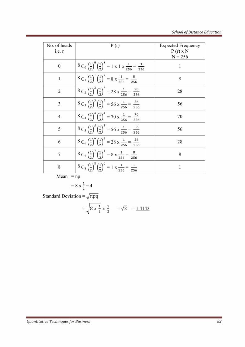
School of Distance Education
Quantitative Techniques for Business 82
No. of heads
i.e. r P (r) Expected Frequency
P (r) x N N = 256
0 8 C0 0 8
= 1 x 1 x = 1
1 8 C1 1 7
= 8 x = 8
2 8 C2 2 6
= 28 x = 28
3 8 C3 3 5
= 56 x = 56
4 8 C4 4 4
= 70 x = 70
5 8 C5 5 3
= 56 x = 56
6 8 C6 6 2
= 28 x = 28
7 8 C7 7 1
= 8 x = 8
8 8 C8 8 0
= 1 x = 1
Mean = np
= 8 x = 4
Standard Deviation =
= 8 = √2 = 1.4142
School of Distance Education
Quantitative Techniques for Business 83
CHAPTER - 7
POISSON DISTRIBUTION
Meaning and Definition:
Poisson Distribution is a limiting form of Binomial Distribution. In Binomial Distribution, the total number of trials are known previously. But in certain real life situations, it may be impossible to count the total number of times a particular event occurs or does not occur. In such cases Poisson Distribution is more suitable.
Poison Distribution is a discrete probability distribution. It was originated by Simeon Denis Poisson.
The Poisson Distribution is defined as:-
p (r) = .!
Where r = random variable (i.e., number of success in ‘n’ trials.
e = 2.7183
m = mean of poisson distribution
Properties of Poisson Distribution
1. Poisson Distribution is a discrete probability distribution.
2. Poisson Distribution has a single parameter ‘m’. When ‘m’ is known all the terms can be found out.
3. It is a positively skewed distribution.
4. Mean and Varriance of Poisson Distribution are equal to ‘m’.
5. In Poisson Distribution, the number of success is relatively small.
6. The standard deviation of Poisson Distribution is √ .
Practical situations where Poisson Distribution can be used
1. To count the number of telephone calls arising at a telephone switch board in a unit of time.
2. To count the number of customers arising at the super market in a unit of time.
3. To count the number of defects in Statistical Quality Control.
4. To count the number of bacterias per unit.
5. To count the number of defectives in a park of manufactured goods.
6. To count the number of persons dying due to heart attack in a year.
7. To count the number of accidents taking place in a day on a busy road.
School of Distance Education
Quantitative Techniques for Business 84
Qn: A fruit seller, from his past experience, knows that 3% of apples in each basket will be defectives. What is the probability that exactly 4 apples will be defective in a given basket?
Sol: p (r) = .!
m = 3
∴ p (r = 4) = . !
= .
= .
= 0.16804
Qn: It is known from the past experience that in a certain plant, there are on an average four industrial accidents per year. Find the probability that in a given year there will be less than four accidents. Assume poisson distribution.
Sol: p (r<4) = p(r = 0 or 1 or 2 or 3)
= p (r = 0) + p (r =1) + p (r = 2) + p (r = 3)
P (r) = .!
m = 4
∴ p (r = 0) = . !
= . = 0.01832
p (r = 1) = . !
= . = 0.07328
p (r = 2) = . !
= .
= 0.14656
p (r = 3) = . !
= .
= 0.19541
∴ p (r < 4) = 0.01832 + 0.07328 + 0.14656 + 0.19541
= 0.43357
Qn: Out of 500 items selected for inspection, 0.2% are found to be defective. Find how many lots will contain exactly no defective if there are 1000 lots.
Sol: p = 0.2% = 0.002
n = 500
m = np = 500 x 0.002 = 1

School of Distance Education
Quantitative Techniques for Business 85
p (r) = .!
p (r = 0) = . !
= . = 0.36788
∴ Number of lots containing no defectives if there are 1000 lots = 0.36788 x 1000
= 367.88
= 368
Qn: In a factory manufacturing optical lenses, there is a small chance of for any one lense to be defective. The lenses are supplied in packets of 10. Use Poisson Distribution to calculate the approximate number of packets containing (1) one defective (2) no defective in a consignment of 20,000 packets. You are given that e-0.02 = 0.9802.
Sol: n = 10
p = probability of manufacturing defective lense = = 0.002
m = np = 10 x 0.002 = 0.02
p (r) = . !
p (r = 1) = . .
! = . .
= 0.019604
∴ No. of packets containing one defective lense = 0.019604 x 20,000
= 392
p (r = 0) = . .
! = .
= 0.9802
∴ No. of packets containing no defective lense = 0.9892 x 20,000
= 19604
Qn: A Systematic sample of 100 pages was taken from a dictionary and the observed frequency distribution of foreign words per page was found to be as follows:
No. of foreign words per page (x) : 0 1 2 3 4 5 6
Frequency (f) : 48 27 12 7 4 1 1
Calculate the expected frequencies using Poisson Distribution.
Sol: p (r) = . !
Here first we have to find out ‘m’.
School of Distance Education
Quantitative Techniques for Business 86
Computation of mean (m)
x f fx
0 48 0
1 27 27
2 12 24
3 7 21
4 4 16
5 1 5
6 1 6
N = 100 Σfx = 99
x = Σ = = 0.99
∴ m = 0.99
∴ Poisson Distribution = . .
!
Computation of expected frequencies
x p (x) Expected frequency Nx p(x)
0 . .!
= 0.3716 100 x 0.3716 = 37.2
1 . .!
= 0.3679 100 x 0.3679 = 36.8
2 . .!
= 0.1821 100 x 0.1821 = 18.21
3 .99 .!
= 0.0601 100 x 0.0601 = 6
4 . .!
= 0.0149 100 x 0.0149 = 1.5
5 . .!
= 0.0029 100 x 0.0029 = 0.3
6 . .!
= 0.0005 100 x 0.0005 = 0.1
Hence, the expected frequencies of this Poisson Distribution are:-
No. of foreign words per page : 0 1 2 3 4 5 6
Expected frequencies (Rounded): 37 37 18 6 2 0 0
School of Distance Education
Quantitative Techniques for Business 87
CHAPTER - 8
NORMAL DISTRIBUTION
The normal distribution is a continuous probability distribution. It was first developed by De-Moivre in 1733 as limiting form of binomial distribution. Fundamental importance of normal distribution is that many populations seem to follow approximately a pattern of distribution as described by normal distribution. Numerous phenomena such as the age distribution of any species, height of adult persons, intelligent test scores of students, etc. are considered to be normally distributed.
Definition of Normal Distribution
A continuous random variable ‘X’ is said to follow Normal Distribution if its probability function is:
P (X) = √ σ
x e ( µσ
) 2
π = 3.146
e = 2.71828
µ = mean of the distribution
σ = standard deviation of the distribution
Properties of Normal Distribution (Normal Curve)
1. Normal distribution is a continuous distribution. 2. Normal curve is symmetrical about the mean. 3. Both sides of normal curve coincide exactly. 4. Normal curve is a bell shaped curve. 5. Mean, Median and Mode coincide at the centre of the curve. 6. Quantities are equi-distant from median.
Q3 – Q2 = Q2 – Q1 7. Normal curve is asymptotic to the base line. 8. Total area under a normal curve is 100%. 9. The ordinate at the mean divide the whole area under a normal curve into two equal parts.
(50% on either side). 10. The height of normal curve is at its maximum at the mean. 11. The normal curve is unimodel, i.e., it has only one mode. 12. Normal curve is mesokurtic. 13. No portion of normal curve lies below the x-axis. 14. Theoretically, the range of normal curve is – α to + α . But practically the range is
µ - 3σ to µ + 3σ.
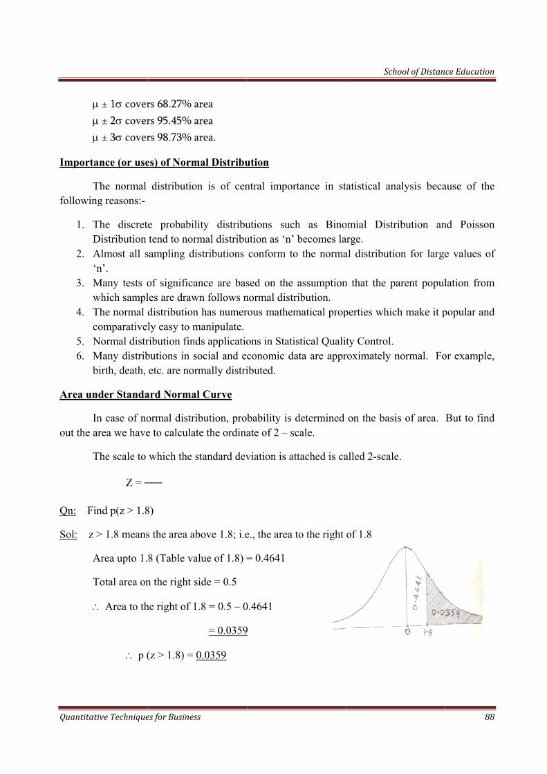
Quantitati
15. Tµµµ
Importa
Tfollowing
1. TD
2. A‘n
3. Mw
4. Tco
5. N6. M
bi
Area und
Inout the ar
T
Qn: Fin
Sol: z >
A
T
∴
ive Technique
The area und ± 1σ cover ± 2σ cover ± 3σ cover
nce (or use
The normal g reasons:-
The discreteDistribution Almost all sn’.
Many tests owhich samplThe normal domparativel
Normal distrMany distrib
irth, death,
der Standa
n case of norea we have
The scale to
Z =
nd p(z > 1.8
> 1.8 means
Area upto 1.8
Total area on
Area to th
∴ p (
es for Business
der normal crs 68.27% ars 95.45% ars 98.73% a
es) of Norm
distribution
e probabilitend to norm
sampling di
of significales are drawdistributionly easy to mribution findbutions in soetc. are nor
ard Normal
ormal distrie to calculat
which the s
8)
s the area ab
8 (Table va
n the right s
he right of 1
(z > 1.8) = 0
s
curve is distarea area area.
mal Distribu
n is of cen
ity distribumal distribustributions
ance are baswn follows nn has numermanipulate.ds applicatioocial and ec
rmally distri
l Curve
bution, probte the ordina
standard dev
bove 1.8; i.e
alue of 1.8) =
ide = 0.5
.8 = 0.5 – 0
= 0.0359
0.0359
tributed as f
ution
ntral import
utions suchution as ‘n’ conform to
sed on the normal distrrous mathem
ons in Statisconomic daibuted.
bability is date of 2 – sc
viation is at
e., the area t
= 0.4641
0.4641
9
follows:
tance in st
h as Binobecomes la
o the norma
assumptionribution. matical prop
stical Qualitata are appr
determined cale.
ttached is ca
to the right
Sch
atistical an
omial Distrarge. al distributio
n that the p
perties whic
ty Control. roximately n
on the basi
alled 2-scale
of 1.8
hool of Distan
nalysis beca
ribution an
on for large
arent popul
ch make it p
normal. Fo
is of area.
e.
ce Education
88
ause of the
nd Poisson
e values of
lation from
popular and
or example,
But to find
8
n
f
m
d
d
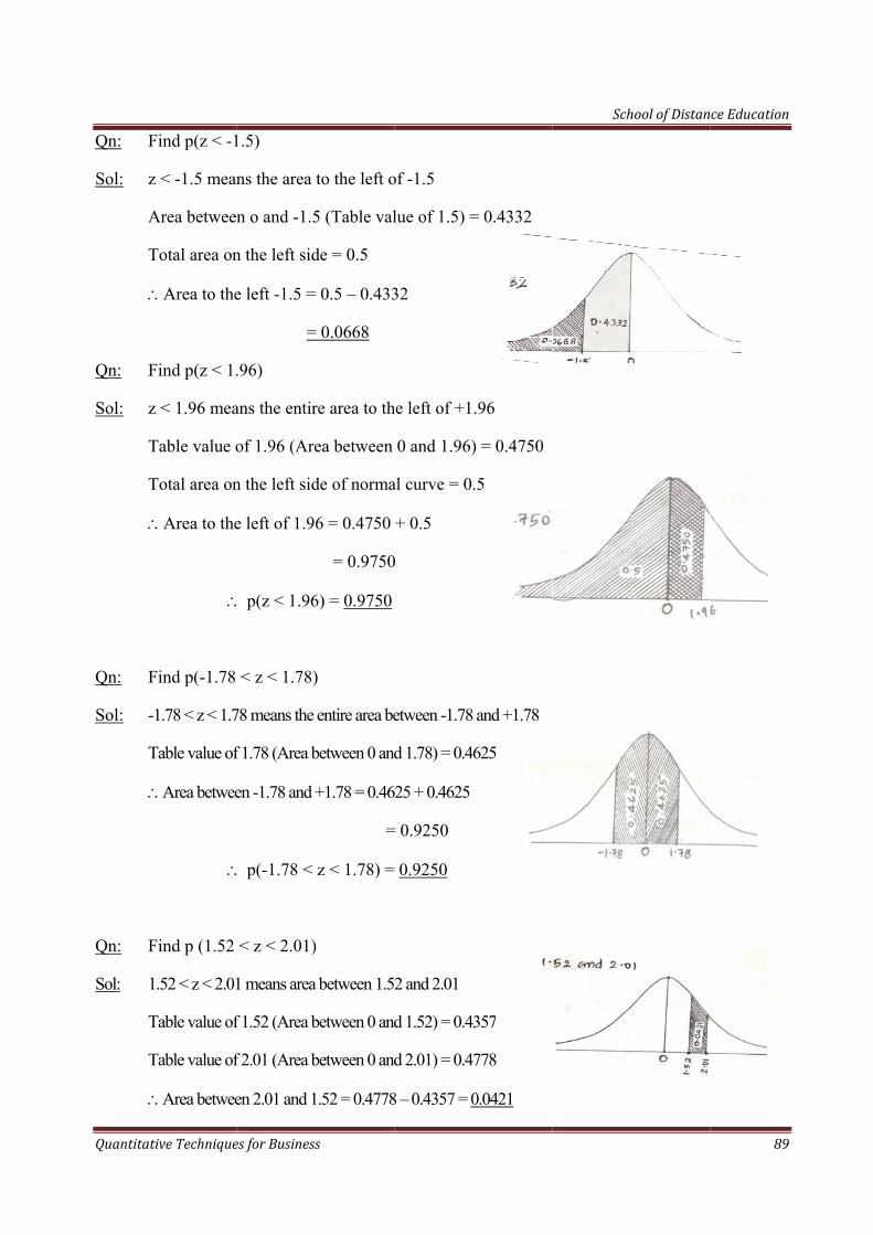
Quantitati
Qn: F
Sol: z
A
T
∴
Qn: F
Sol: z
T
T
∴
Qn: F
Sol: -1
T
∴
Qn: F
Sol: 1.
T
T
∴
ive Technique
ind p(z < -1
< -1.5 mean
Area between
Total area on
Area to the
ind p(z < 1.
< 1.96 mea
Table value o
Total area on
Area to the
∴
ind p(-1.78
1.78 < z < 1.7
Table value of
Area betwee
∴
ind p (1.52
.52 < z < 2.01
Table value of
Table value of
Area betwee
es for Business
1.5)
ns the area
n o and -1.5
n the left sid
e left -1.5 =
=
.96)
ans the entir
of 1.96 (Are
n the left sid
e left of 1.96
p(z < 1.96
< z < 1.78)
78 means the
f 1.78 (Area b
en -1.78 and +
p(-1.78 <
< z < 2.01)
1 means area
f 1.52 (Area b
f 2.01 (Area b
en 2.01 and 1
s
to the left o
5 (Table val
de = 0.5
= 0.5 – 0.433
= 0.0668
re area to th
ea between
de of norma
6 = 0.4750
= 0.9750
6) = 0.9750
)
entire area be
between 0 and
+1.78 = 0.46
=
z < 1.78) =
)
a between 1.5
between 0 and
between 0 and
1.52 = 0.4778
of -1.5
lue of 1.5) =
32
he left of +1
0 and 1.96)
al curve = 0.
+ 0.5
0
etween -1.78
d 1.78) = 0.46
625 + 0.4625
= 0.9250
0.9250
2 and 2.01
d 1.52) = 0.43
d 2.01) = 0.47
8 – 0.4357 = 0
= 0.4332
.96
) = 0.4750
.5
and +1.78
625
357
778
0.0421
Schhool of Distance Education
89
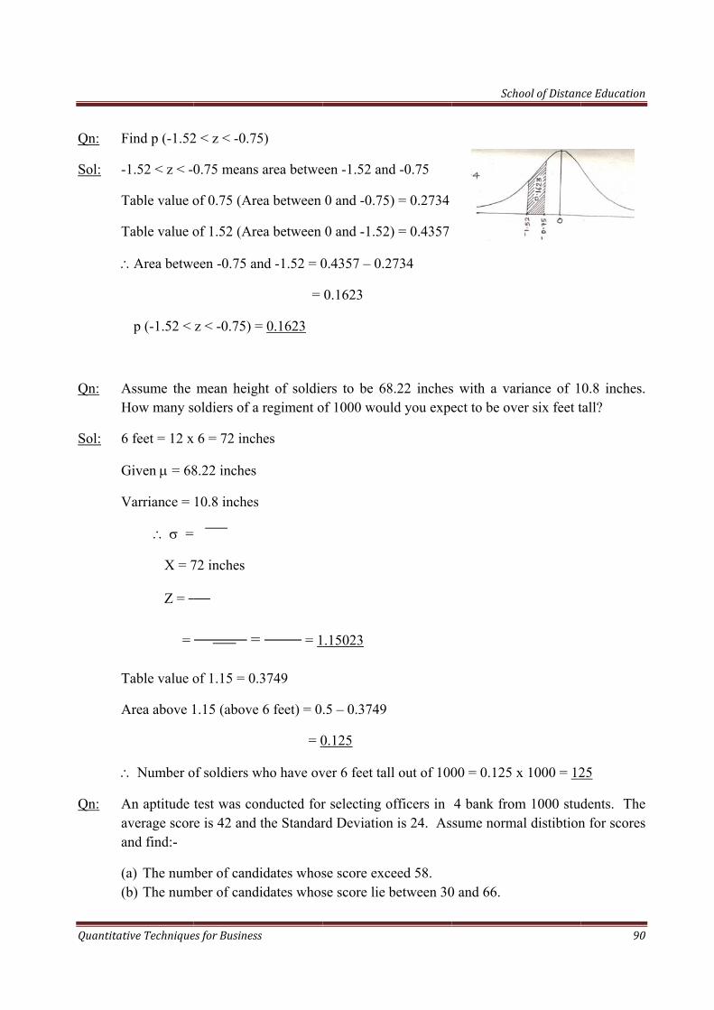
Quantitati
Qn: F
Sol: -1
T
T
∴
Qn: AH
Sol: 6
G
V
T
A
∴
Qn: Aavan
(a(b
ive Technique
ind p (-1.52
1.52 < z < -0
Table value o
Table value o
Area betw
p (-1.52 <
Assume the How many s
feet = 12 x
Given µ = 68
Varriance =
∴ σ =
X = 7
Z =
=
Table value o
Area above 1
Number o
An aptitude verage scornd find:-
a) The numb) The num
es for Business
2 < z < -0.75
0.75 means
of 0.75 (Are
of 1.52 (Are
een -0.75 an
z < -0.75) =
mean heigholdiers of a
x 6 = 72 inch
8.22 inches
10.8 inches
72 inches
=
of 1.15 = 0.
1.15 (above
of soldiers w
test was core is 42 and
mber of candmber of cand
s
5)
area betwe
ea between
ea between
nd -1.52 = 0
=
= 0.1623
ht of soldiea regiment o
hes
s
= = 1
3749
e 6 feet) = 0
= 0
who have ov
onducted forthe Standar
didates whosdidates whos
een -1.52 an
0 and -0.75
0 and -1.52
0.4357 – 0.2
0.1623
ers to be 68of 1000 wou
.15023
.5 – 0.3749
0.125
ver 6 feet tal
r selecting ord Deviation
se score excse score lie
nd -0.75
5) = 0.2734
2) = 0.4357
2734
8.22 inchesuld you expe
ll out of 100
officers in n is 24. As
ceed 58. between 30
Sch
s with a varect to be ov
00 = 0.125 x
4 bank fromsume norm
0 and 66.
hool of Distan
riance of 1ver six feet t
x 1000 = 12
m 1000 stumal distibtion
ce Education
90
0.8 inches.tall?
25
dents. Then for scores
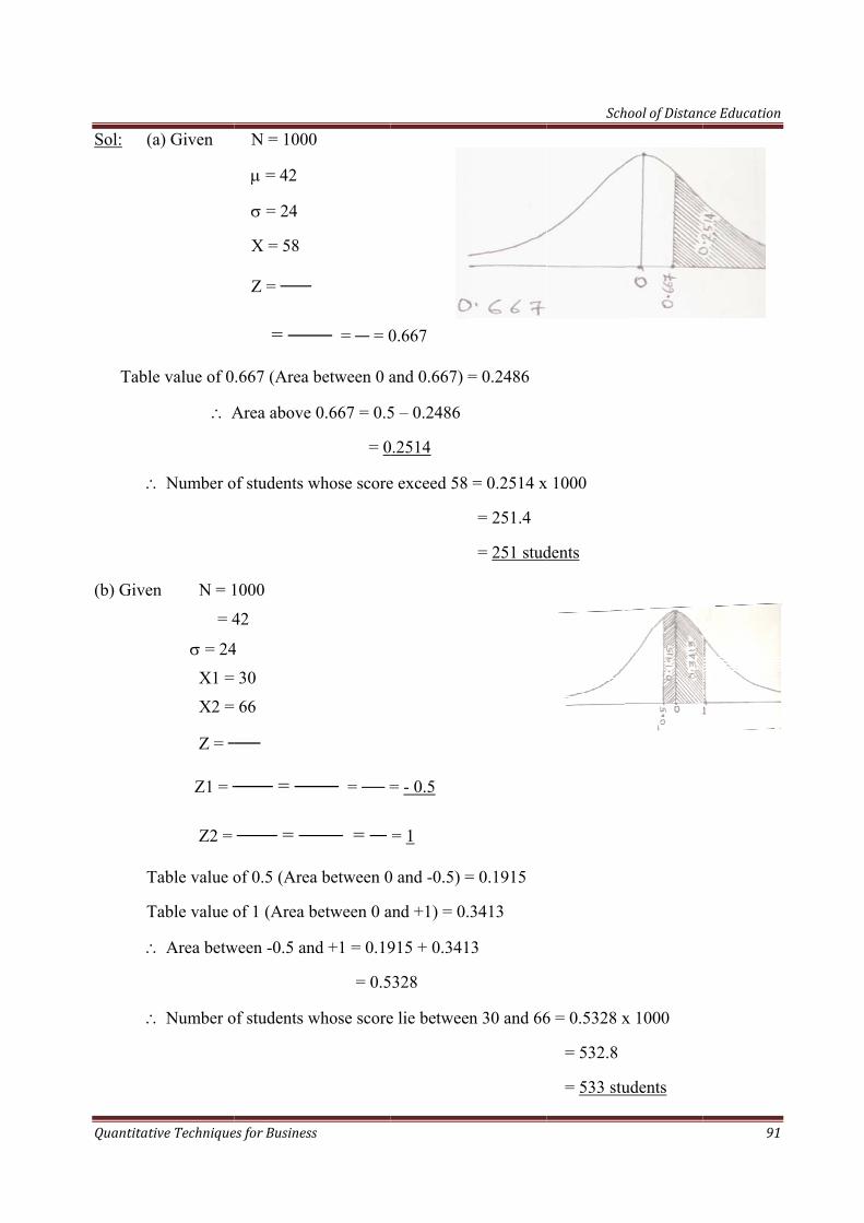
Quantitati
Sol: (a
Table
∴
(b) Given
T
T
∴
∴
ive Technique
a) Given
e value of 0
∴ A
Number o
n N = 1
= 4
σ = 24
X1 =
X2 =
Z =
Z1 =
Z2 =
Table value o
Table value o
Area betw
Number o
es for Business
N = 1000
µ = 42
σ = 24
X = 58
Z =
=
.667 (Area
Area above
of students w
1000
42
4
30
66
=
=
of 0.5 (Area
of 1 (Area b
ween -0.5 an
of students w
s
0
= = 0
between 0 a
0.667 = 0.5
= 0
whose score
= =
=
a between 0
between 0 a
nd +1 = 0.19
= 0.5
whose score
0.667
and 0.667) =
5 – 0.2486
0.2514
e exceed 58
= - 0.5
= 1
0 and -0.5) =
and +1) = 0.
915 + 0.341
5328
e lie betwee
= 0.2486
= 0.2514 x
= 251.4
= 251 stud
= 0.1915
3413
13
n 30 and 66
Sch
x 1000
dents
6 = 0.5328 x
= 532.8
= 533 stu
hool of Distan
x 1000
udents
ce Education
91
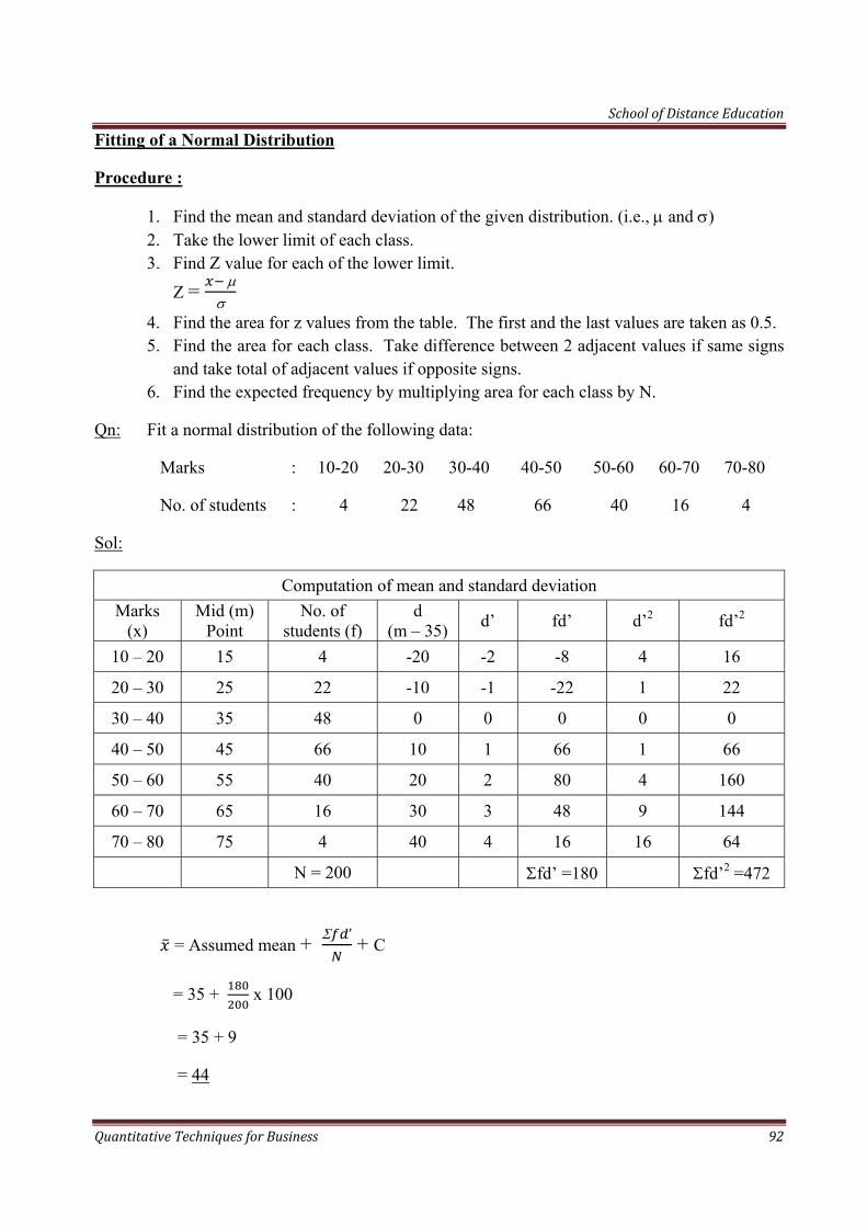
School of Distance Education
Quantitative Techniques for Business 92
Fitting of a Normal Distribution
Procedure :
1. Find the mean and standard deviation of the given distribution. (i.e., µ and σ) 2. Take the lower limit of each class. 3. Find Z value for each of the lower limit.
Z = µσ
4. Find the area for z values from the table. The first and the last values are taken as 0.5. 5. Find the area for each class. Take difference between 2 adjacent values if same signs
and take total of adjacent values if opposite signs. 6. Find the expected frequency by multiplying area for each class by N.
Qn: Fit a normal distribution of the following data:
Marks : 10-20 20-30 30-40 40-50 50-60 60-70 70-80
No. of students : 4 22 48 66 40 16 4
Sol:
Computation of mean and standard deviation Marks
(x) Mid (m)
Point No. of
students (f) d
(m – 35) d’ fd’ d’2 fd’2
10 – 20 15 4 -20 -2 -8 4 16
20 – 30 25 22 -10 -1 -22 1 22
30 – 40 35 48 0 0 0 0 0
40 – 50 45 66 10 1 66 1 66
50 – 60 55 40 20 2 80 4 160
60 – 70 65 16 30 3 48 9 144
70 – 80 75 4 40 4 16 16 64
N = 200 Σfd’ =180 Σfd’2 =472
= Assumed mean + Σ ’ + C
= 35 + x 100
= 35 + 9
= 44
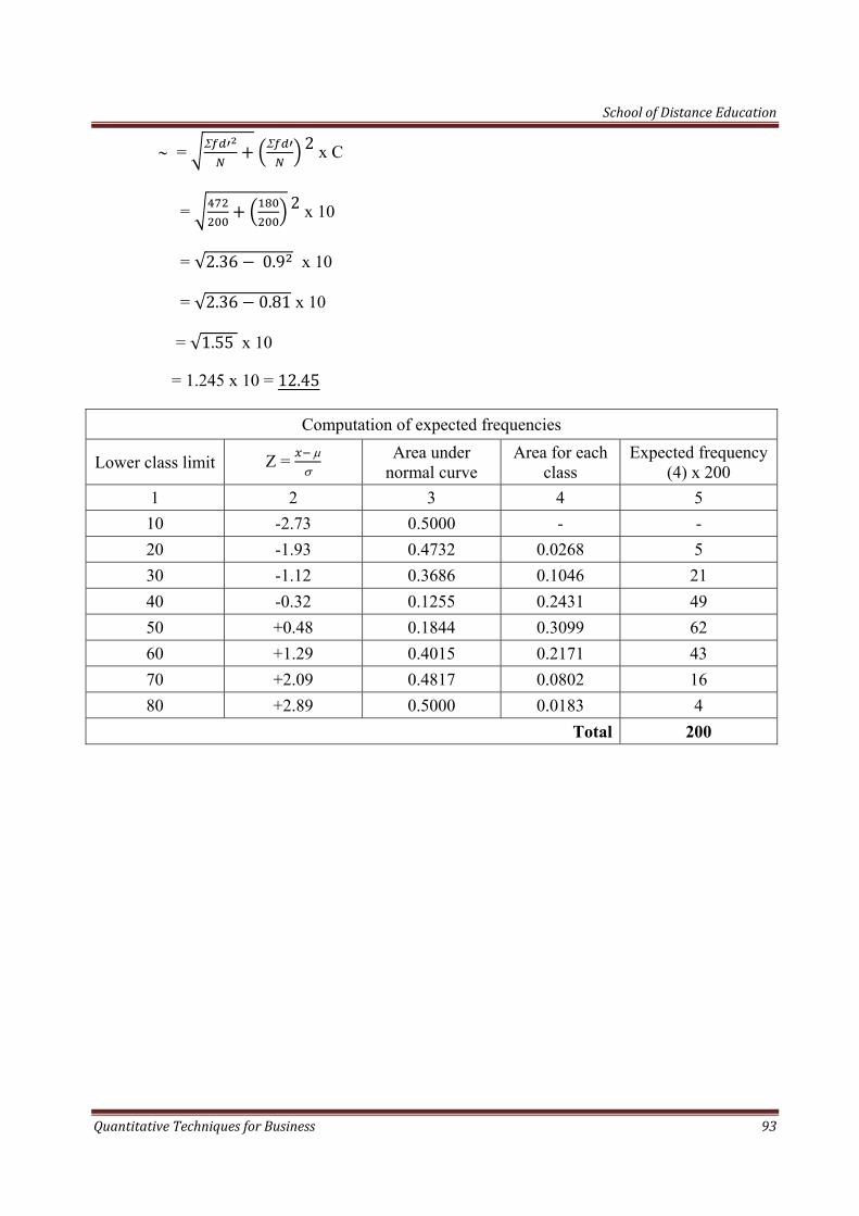
School of Distance Education
Quantitative Techniques for Business 93
∼ = Σ Σ 2 x C
= 2 x 10
= √2.36 0.9 x 10
= √2.36 0.81 x 10
= √1.55 x 10
= 1.245 x 10 = 12.45
Computation of expected frequencies
Lower class limit Z = µσ
Area under normal curve
Area for each class
Expected frequency (4) x 200
1 2 3 4 5 10 -2.73 0.5000 - - 20 -1.93 0.4732 0.0268 5 30 -1.12 0.3686 0.1046 21 40 -0.32 0.1255 0.2431 49 50 +0.48 0.1844 0.3099 62 60 +1.29 0.4015 0.2171 43 70 +2.09 0.4817 0.0802 16 80 +2.89 0.5000 0.0183 4
Total 200
School of Distance Education
Quantitative Techniques for Business 94
CHAPTER - 9
TESTING OF HYPOTHESIS
Statistical Inference:
Statistical inference refers to the process of selecting and using a sample statistic to draw conclusions about the population parameter. Statistical inference deals with two types of problems.
They are:-
1. Testing of Hypothesis
2. Estimation
Hypothesis:
Hypothesis is a statement subject to verification. More precisely, it is a quantitative statement about a population, the validity of which remains to be tested. In other words, hypothesis is an assumption made about a population parameter.
Testing of Hypothesis:
Testing of hypothesis is a process of examining whether the hypothesis formulated by the researcher is valid or not. The main objective of hypothesis testing is whether to accept or reject the hypothesis.
Procedure for Testing of Hypothesis:
The various steps in testing of hypothesis involves the following :-
1. Set Up a Hypothesis:
The first step in testing of hypothesis is to set p a hypothesis about population parameter. Normally, the researcher has to fix two types of hypothesis. They are null hypothesis and alternative hypothesis.
Null Hypothesis:-
Null hypothesis is the original hypothesis. It states that there is no significant difference between the sample and population regarding a particular matter under consideration. The word “null” means ‘invalid’ of ‘void’ or ‘amounting to nothing’. Null hypothesis is denoted by Ho. For example, suppose we want to test whether a medicine is effective in curing cancer. Hence, the null hypothesis will be stated as follows:-
H0: The medicine is not effective in curing cancer (i.e., there is no significant difference between the given medicine and other medicines in curing cancer disease.)
Alternative Hypothesis:- Any hypothesis other than null hypothesis is called alternative hypothesis. When a null hypothesis is rejected, we accept the other hypothesis, known as alternative hypothesis. Alternative hypothesis is denoted by H1. In the above example, the alternative hypothesis may be stated as follows:-
School of Distance Education
Quantitative Techniques for Business 95
H1: The medicine is effective in curing cancer. (i.e., there is significant difference between the given medicine and other medicines in curing cancer disease.)
2. Set up a suitable level of significance:
After setting up the hypothesis, the researcher has to set up a suitable level of significance. The level of significance is the probability with which we may reject a null hypothesis when it is true. For example, if level of significance is 5%, it means that in the long run, the researcher is rejecting true null hypothesis 5 times out of every 100 times. Level of significance is denoted by α (alpha).
α = Probability of rejecting H0 when it is true.
Generally, the level of significance is fixed at 1% or 5%.
3. Decide a test criterion:
The third step in testing of hypothesis is to select an appropriate test criterion. Commonly used tests are z-test, t-test, X2 – test, F-test, etc.
4. Calculation of test statistic:
The next step is to calculate the value of the test statistic using appropriate formula. The general fromfor computing the value of test statistic is:-
Value of Test statistic = Difference
Standard Error
5. Making Decision:
Finally, we may draw conclusions and take decisions. The decision may be either to accept or reject the null hypothesis.
If the calculated value is more than the table value, we reject the null hypothesis and accept the alternative hypothesis.
If the calculated value is less than the table value, we accept the null hypothesis.
Sampling Distribution
The distribution of all possible values which can be assumed by some statistic, computed from samples of the same size randomly drawn from the same population is called Sampling distribution of that statistic.
Standard Error (S.E)
Standard Error is the standard deviation of the sampling distribution of a statistic. Standard error plays a very important role in the large sample theory. The following are the important uses of standard errors:-
1. Standard Error is used for testing a given hypothesis
School of Distance Education
Quantitative Techniques for Business 96
2. S.E. gives an idea about the reliability of a sample, because the reciprocal of S.E. is a measure of reliability of the sample.
3. S.E. can be used to determine the confidence limits within which the population parameters are expected to lie.
Test Statistic
The decision to accept or to reject a null hypothesis is made on the basis of a statistic computed from the sample. Such a statistic is called the test statistic. There are different types of test statistics. All these test statistics can be classified into two groups. They are
a. Parametric Tests
b. Non-Parametric Tests
PARAMETRIC TESTS
The statistical tests based on the assumption that population or population parameter is normally distributed are called parametric tests. The important parametric tests are:-
1. z-test
2. t-test
3. f-test
Z-test:
Z-test is applied when the test statistic follows normal distribution. It was developed by Prof.R.A.Fisher. The following are the important uses of z-test:-
1. To test the population mean when the sample is large or when the population standard deviation is known.
2. To test the equality of two sample means when the samples are large or when the population standard deviation is known.
3. To test the population proportion.
4. To test the equality of two sample proportions.
5. To test the population standard deviation when the sample is large.
6. To test the equality of two sample standard deviations when the samples are large or when population standard deviations are known.
7. To test the equality of correlation coefficients.
Z-test is used in testing of hypothesis on the basis of some assumptions. The important assumptions in z-test are:-
1. Sampling distribution of test statistic is normal.
School of Distance Education
Quantitative Techniques for Business 97
2. Sample statistics are dose the population parameter and therefore, for finding standard error, sample statistics are used in place where population parameters are to be used.
T-test:
t-distribution was originated by W.S.Gosset in the early 1900.
t-test is applied when the test statistic follows t-distribution.
Uses of t-test are:-
1. To test the population mean when the sample is small and the population s.D.is unknown.
2. To test the equality of two sample means when the samples are small and population S.D. is unknown.
3. To test the difference in values of two dependent samples.
4. To test the significance of correlation coefficients.
The following are the important assumptions in t-test:-
1. The population from which the sample drawn is normal.
2. The sample observations are independent.
3. The population S.D.is known.
4. When the equality of two population means is tested, the samples are assumed to be independent and the population variance are assumed to be equal and unknown.
F-test:
F-test is used to determined whether two independent estimates of population variance significantly differ or to establish both have come from the same population. For carrying out the test of significance, we calculate a ration, called F-ratio. F-test is named in honour of the great statistician R.A.Fisher. It is also called Variance Ration Test.
F-ratio is defined as follows:-
F =
where S =
S =
While calculating F-ratio, the numerator is the greater variance and denominator is the smaller variance. So,
F = Greater Variance
Smaller Variance
School of Distance Education
Quantitative Techniques for Business 98
Uses of F-distribution:-
1. To test the equality of variances of two populations.
2. To test the equality of means of three or more populations.
3. To test the linearity of regression
Assumptions of F-distribution:-
1. The values in each group are normally distributed.
2. The variance within each group should be equal for all groups. ( …)
3. The error (Variation of each value around its own group mean) should be independent for each value.
TYPES OF ERRORS IN TESTING OF HYPOTHESIS:
In any test of hypothesis, the decision is to accept or reject a null hypothesis. The four possibilities of the decision are:-
1. Accepting a null hypothesis when it is true.
2. Rejecting a null hypothesis when it is false.
3. Rejecting a null hypothesis when it is true.
4. Accepting a null hypothesis when it is false.
Out of the above 4 possibilities, 1 and 2 are correct, while 3 and 4 are errors. The error included in the above 3rd possibility is called type I error and that in the 4th possibility is called type II error.
Type I Error
The error committed by rejecting a null hypothesis when it is true, is called Type I error. The probability of committing Type I error is denoted by α (alpha).
α = Prob. (Type I error)
= Prob. (Rejecting H0 when it is true)
Type II Error
The error committed by accepting a null hypothesis when it is false is called Type II error. The probability of committing Type II error is denoted by β (beta).
β = Prob. (Type II error)
β = Prob. (Accepting H0 when it is false)
Small and Large samples
The size of sample is 30 or less than 30, the sample is called small sample.
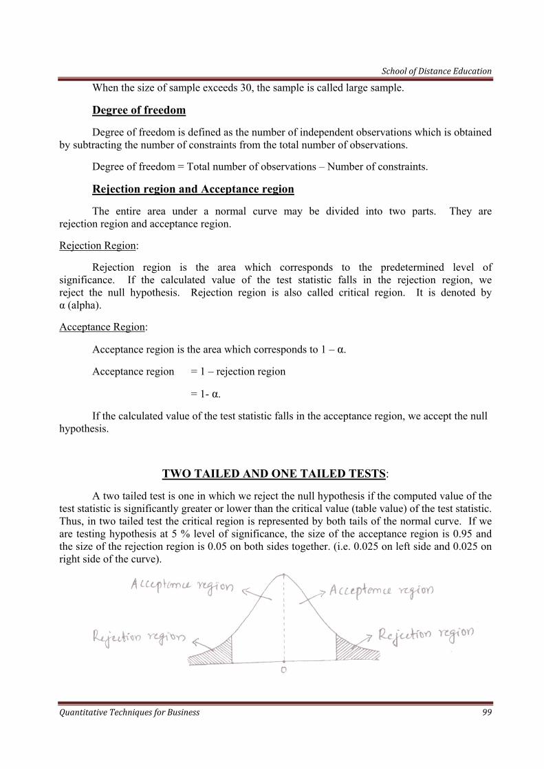
School of Distance Education
Quantitative Techniques for Business 99
When the size of sample exceeds 30, the sample is called large sample.
Degree of freedom
Degree of freedom is defined as the number of independent observations which is obtained by subtracting the number of constraints from the total number of observations.
Degree of freedom = Total number of observations – Number of constraints.
Rejection region and Acceptance region
The entire area under a normal curve may be divided into two parts. They are rejection region and acceptance region.
Rejection Region:
Rejection region is the area which corresponds to the predetermined level of significance. If the calculated value of the test statistic falls in the rejection region, we reject the null hypothesis. Rejection region is also called critical region. It is denoted by α (alpha).
Acceptance Region:
Acceptance region is the area which corresponds to 1 – α.
Acceptance region = 1 – rejection region
= 1- α.
If the calculated value of the test statistic falls in the acceptance region, we accept the null hypothesis.
TWO TAILED AND ONE TAILED TESTS:
A two tailed test is one in which we reject the null hypothesis if the computed value of the test statistic is significantly greater or lower than the critical value (table value) of the test statistic. Thus, in two tailed test the critical region is represented by both tails of the normal curve. If we are testing hypothesis at 5 % level of significance, the size of the acceptance region is 0.95 and the size of the rejection region is 0.05 on both sides together. (i.e. 0.025 on left side and 0.025 on right side of the curve).
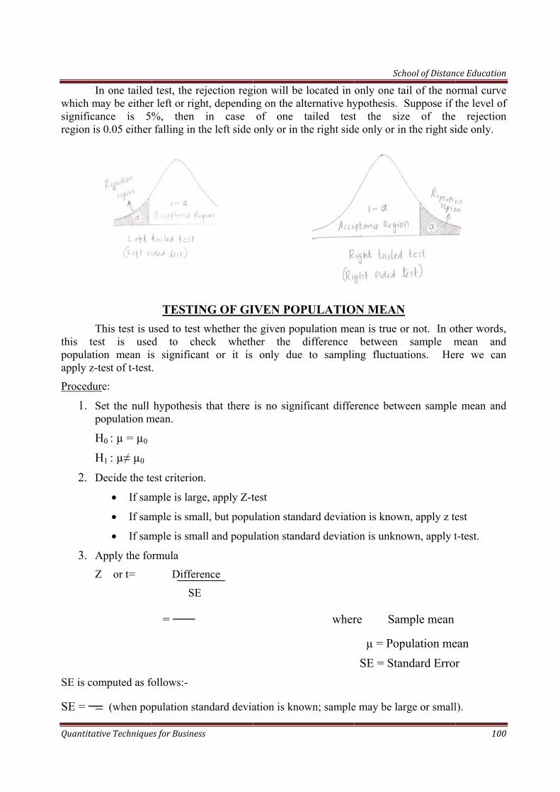
Quantitati
Inwhich masignificanregion is
Tthis tespopulatioapply z-t
Procedur
1. Spo
HH
2. D
3. A
Z
SE is com
SE =
ive Technique
n one taileday be eithernce is 5%0.05 either
This test is ust is useon mean isest of t-test
re:
et the null opulation m
H0 : µ = µ0
H1 : µ≠ µ0
Decide the te
• If sam
• If sam
• If sam
Apply the fo
Z or t =
mputed as fo
(when pop
es for Business
d test, the rer left or righ%, then falling in th
TESTINused to test d to ches significan.
hypothesis mean.
est criterion
mple is large
mple is sma
mple is sma
rmula
Differe
SE
=
follows:-
pulation sta
s
ejection reght, dependinin case
he left side
NG OF GIwhether the
eck whethnt or it is
that there
n.
e, apply Z-t
all, but popu
all and popu
ence
andard devia
ion will be ng on the al
of one only or in th
IVEN POPe given popher the d
only due
is no signi
test
ulation stand
ulation stand
ation is kno
located in lternative hytailed testhe right sid
PULATIOpulation medifference
to sampli
ficant diffe
dard deviati
dard deviatio
wher
own; sample
Sch
only one taypothesis. St the siz
de only or in
ON MEANan is true o
between ng fluctuat
rence betw
ion is known
on is unkno
re Sam
µ = Pop SE = Stan
e may be lar
hool of Distan
ail of the noSuppose if te of the
n the right si
or not. In ot
sample mtions. Her
ween sample
n, apply z te
own, apply t
mple mean
ulation mendard Error
rge or small
ce Education
100
ormal curvethe level of rejectionide only.
ther words,mean andre we can
e mean and
est
t-test.
ean r
l).
f n
d n
d
School of Distance Education
Quantitative Techniques for Business 101
SE = √
(when population standard deviation is unknown & sample is large).
SE = √
(when population standard deviation is known and sample is small).
where = Population S.D.; S = Sample S.D.; n = Sample size;
4. Fix the degree of freedom.
For Z-test: Infinity
For t-test: n-1
5. Obtain the table value at level of significance for degree of freedom.
6. Decide whether to accept or reject the H0. If calculated value is less than the table value, we accept the H0 otherwise reject it.
Qn: A sample of 900 items is taken from a population with S.D.15. The mean of the sample is 25. Test whether the sample has come from a population with mean 26.8.
Sol: H0 : µ = 26.8 H1 : µ ≠ 26.8 Since sample is large apply z-test.
Z =
=
SE = √
= √
= = 0.5
z = ..
= ..
= 3.6
The value of z at 5% level of significance for infinity d.f. is 1.96. As the calculated value is more than the table value , we reject the H0. There is significant difference sample mean and population mean.
We conclude that the sample has not come from the population with mean 26.8.
Qn. The mean life of 100 bulbs produced by a company is computed to be 1570 hours with S.D. of 120 hours. The company claims that the average life of bulbs produced by the company is 1600 hours. Using 5% level of significance, is the claim acceptable?
Sol: H0 : µ = 1600 H1 : µ ≠ 1600 Since sample is large apply z-test.
Z =
SE = √
= √
= = 12
School of Distance Education
Quantitative Techniques for Business 102
z =
= = 2.5
Table value at 5% level of significance and infinity d.f. is 1.96. As the calculated value is greater than the table value, we reject the H0. There is significant difference between mean life of sample and mean life of population.
Company’s claim is not acceptable
Qn. The price of shares of a company on the different days in a month were found to be 66,65,69,70,69,71,70,63,64 and 68. Discuss whether mean price of shares in the month is 65.
Sol. H0 : µ = 65
H1 : µ ≠ 65
Since small sample, apply t-test.
t =
X = ∑ =
= = 67.5
Computation of Standard deviation
X X-X (X-X)
66 -1.5 2.25
65 -2.5 6.25
69 1.5 2.25
70 2.5 6.25
69 1.5 2.25
71 3.5 12.25
70 2.5 6.25
63 -4.5 20.25
64 -3.5 12.25
68 0.5 0.25
70.50
School of Distance Education
Quantitative Techniques for Business 103
Standard deviation (S) = ∑ 2
= .
= √7.05
= 2.655
S.E = √
= .√
= .√
= .
= 0.885
t = ..
= ..
= 2.8249
Table value at 5% level of significance and 9 d.f. = 2.262. Calculated value is more than table value.
We reject the null hypothesis.
We conclude that the mean price of share in the month is not 65/-.
Qn. The mean height obtained from a random sample of 36 children is 30 inches. The standard deviation of the distribution of height of the population is known to be 1.5 inches. Test the statement that the mean height of the population is 33 inches at 5% level of significance. Also set up 99% confidence limits of the mean height of the population.
Sol. H0 : µ = 33
H1 : µ ≠ 33
Since small sample is large, apply z-test.
z =
X = 30
µ = 33
SE = √
= .
√ =
. = 0.25
z = .
= .
= 12
Table value at 5% level of significance & infinity d.f. = 1.95.
Calculated value is greater than table value.

School of Distance Education
Quantitative Techniques for Business 104
We reject the H0
We conclude that this mean height of population is not 33 inches.
b 99% confidence level = 1% significance level.
Table value of Z at 1% level of = 2.576 ]] significance and infinity d.f.
Limits of Population = X 2.576 SE
= 30 (2.576 x 0.25)
= 30 0.644
= 29.356 and 30.644
Qn. An investigation of a sample of 64 BBA students indicated that the mean time spend on preparing for the examination was 48 months and the S.D. was 15 months. What is the average time spent by all BBA students before they complete their examinations.
Sol. Here, the students are asked to compute the population mean. In other words, the confidence limits of population mean.
Table value of z at 5% level of = 1.96
significance and infinity d.f.
Confidence limits of µ = µ 1.96 SE
S.E. = √
= √
= = 1.875
Confidence Limits of µ = 48 1.96 x 1.875
= 48 3.675
= 44.325 and 51.675
Average time spent by all BBA students before competing their examinations is between 44.325 months and 51.675 months.
Qn. A typist claims that he can take dictations at the rate of more than 120 words per minute. Of the 12 tests given to him, he could perform an average of 135 words with a S.D. of 40. Is his claim valid. (use 1% level of significance).
H0 : µ = 120
H1 : µ 120
Since small sample is large, apply z-test.
t = =
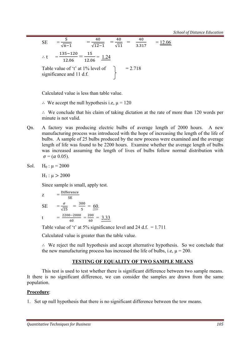
School of Distance Education
Quantitative Techniques for Business 105
SE = √
= √
= √
= .
= 12.06
t = .
= .
= 1.24
Table value of ‘t’ at 1% level of = 2.718 significance and 11 d.f.
Calculated value is less than table value.
We accept the null hypothesis i.e, µ = 120
We conclude that his claim of taking dictation at the rate of more than 120 words per minute is not valid.
Qn. A factory was producing electric bulbs of average length of 2000 hours. A new manufacturing process was introduced with the hope of increasing the length of the life of bulbs. A sample of 25 bulbs produced by the new process were examined and the average length of life was found to be 2200 hours. Examine whether the average length of bulbs was increased assuming the length of lives of bulbs follow normal distribution with = ( 0.05).
Sol. H0 : µ = 2000
H1 : µ 2000
Since sample is small, apply test.
z =
SE = √
= = 60.
t = = = 3.33
Table value of ‘t’ at 5% significance level and 24 d.f. = 1.711
Calculated value is greater than the table value.
We reject the null hypothesis and accept alternative hypothesis. So we conclude that the new manufacturing process has increased the life of bulbs, i.e, µ = 200.
TESTING OF EQUALITY OF TWO SAMPLE MEANS
This test is used to test whether there is significant difference between two sample means. It there is no significant difference, we can consider the samples are drawn from the same population.
Procedure:
1. Set up null hypothesis that there is no significant difference between the tow means.
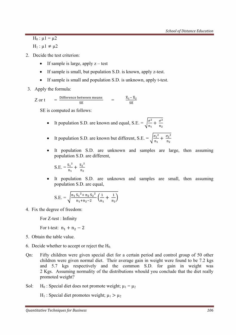
School of Distance Education
Quantitative Techniques for Business 106
H0 : µ1 = µ2
H1 : µ1 µ2
2. Decide the test criterion:
• If sample is large, apply z – test
• If sample is small, but population S.D. is known, apply z-test.
• If sample is small and population S.D. is unknown, apply t-test.
3. Apply the formula:
Z or t = =
SE is computed as follows:
• It population S.D. are known and equal, S.E. =
• It population S.D. are known but different, S.E. =
• It population S.D. are unknown and samples are large, then assuming population S.D. are different,
S.E. =
• It population S.D. are unknown and samples are small, then assuming population S.D. are equal,
S.E. =
4. Fix the degree of freedom:
For Z-test : Infinity
For t-test: n n 2
5. Obtain the table value.
6. Decide whether to accept or reject the H0.
Qn: Fifty children were given special diet for a certain period and control group of 50 other children were given normal diet. Their average gain in weight were found to be 7.2 kgs and 5.7 kgs respectively and the common S.D. for gain in weight was 2 Kgs. Assuming normality of the distributions whould you conclude that the diet really promoted weight?
Sol: H0 : Special diet does not promote weight; µ1 = µ2
H1 : Special diet promotes weight; µ1 µ2
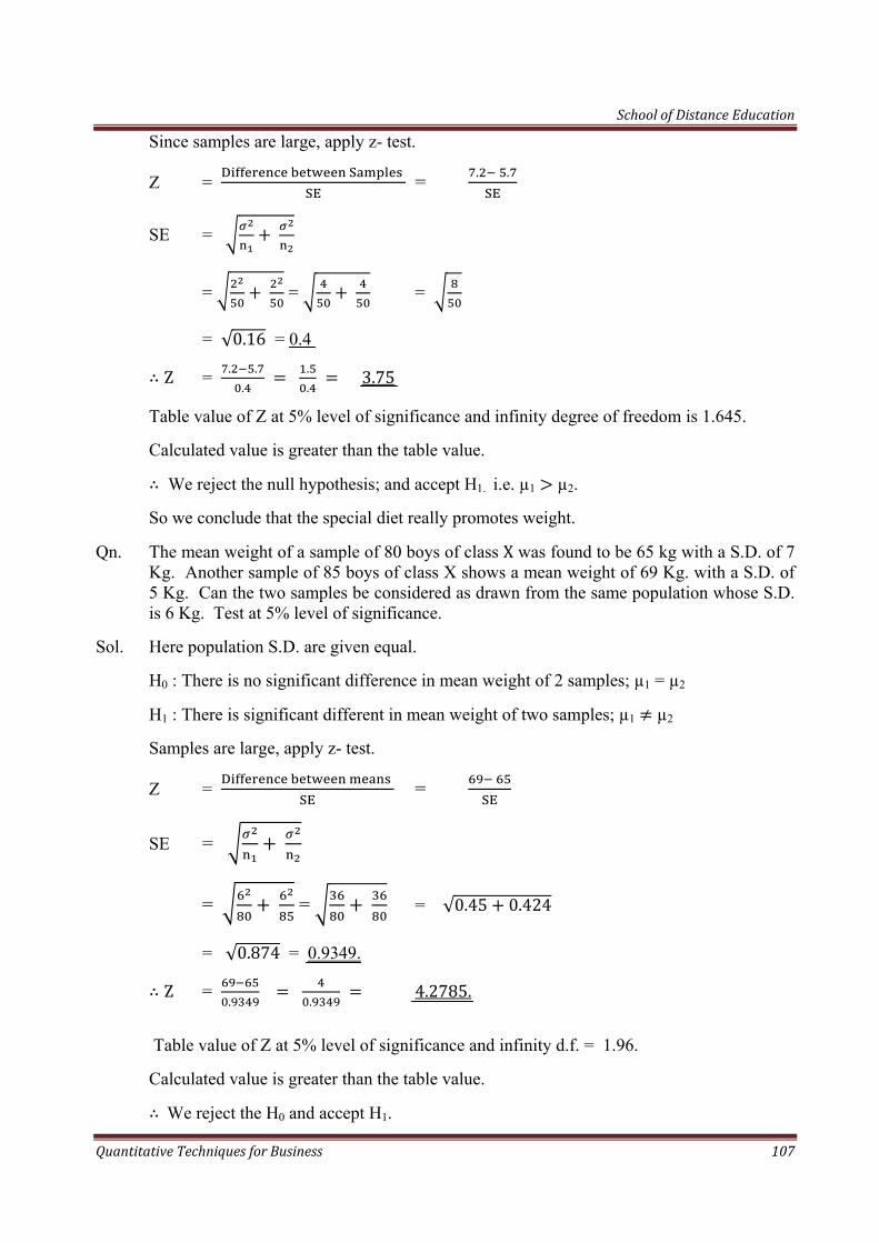
School of Distance Education
Quantitative Techniques for Business 107
Since samples are large, apply z- test.
Z = = . .
SE =
= = =
= √0.16 = 0.4
Z = . ..
.. 3.75
Table value of Z at 5% level of significance and infinity degree of freedom is 1.645.
Calculated value is greater than the table value.
We reject the null hypothesis; and accept H1. i.e. µ1 µ2.
So we conclude that the special diet really promotes weight.
Qn. The mean weight of a sample of 80 boys of class X was found to be 65 kg with a S.D. of 7 Kg. Another sample of 85 boys of class X shows a mean weight of 69 Kg. with a S.D. of 5 Kg. Can the two samples be considered as drawn from the same population whose S.D. is 6 Kg. Test at 5% level of significance.
Sol. Here population S.D. are given equal.
H0 : There is no significant difference in mean weight of 2 samples; µ1 = µ2
H1 : There is significant different in mean weight of two samples; µ1 µ2
Samples are large, apply z- test.
Z = =
SE =
= = = √0.45 0.424
= √0.874 = 0.9349.
Z = .
.
4.2785.
Table value of Z at 5% level of significance and infinity d.f. = 1.96.
Calculated value is greater than the table value.
We reject the H0 and accept H1.
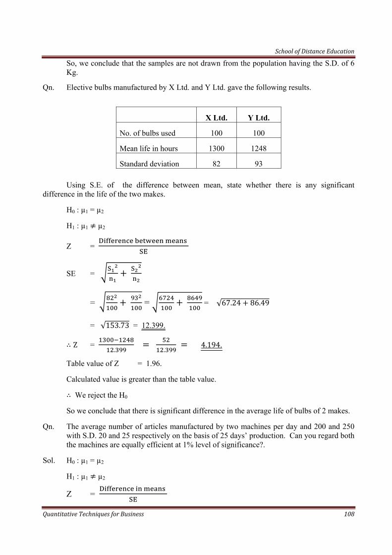
School of Distance Education
Quantitative Techniques for Business 108
So, we conclude that the samples are not drawn from the population having the S.D. of 6 Kg.
Qn. Elective bulbs manufactured by X Ltd. and Y Ltd. gave the following results.
X Ltd. Y Ltd.
No. of bulbs used 100 100
Mean life in hours 1300 1248
Standard deviation 82 93
Using S.E. of the difference between mean, state whether there is any significant difference in the life of the two makes.
H0 : µ1 = µ2
H1 : µ1 µ2
Z =
SE =
= = = √67.24 86.49
= √153.73 = 12.399.
Z = .
.
4.194.
Table value of Z = 1.96.
Calculated value is greater than the table value.
We reject the H0
So we conclude that there is significant difference in the average life of bulbs of 2 makes.
Qn. The average number of articles manufactured by two machines per day and 200 and 250 with S.D. 20 and 25 respectively on the basis of 25 days’ production. Can you regard both the machines are equally efficient at 1% level of significance?.
Sol. H0 : µ1 = µ2
H1 : µ1 µ2
Z =
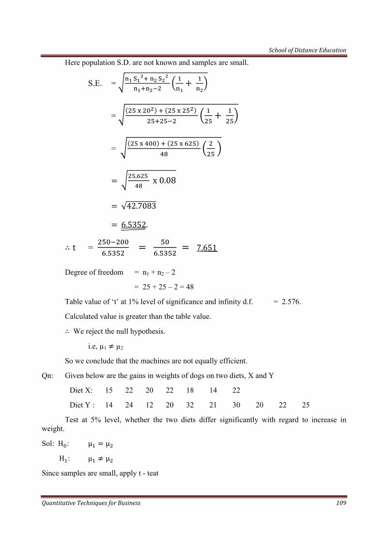
School of Distance Education
Quantitative Techniques for Business 109
Here population S.D. are not known and samples are small.
S.E. =
=
=
, x 0.08
√42.7083
6.5352.
t = .
.
7.651
Degree of freedom = n1 + n2 – 2
= 25 + 25 – 2 = 48
Table value of ‘t’ at 1% level of significance and infinity d.f. = 2.576.
Calculated value is greater than the table value.
We reject the null hypothesis.
i.e, µ1 µ2
So we conclude that the machines are not equally efficient.
Qn: Given below are the gains in weights of dogs on two diets, X and Y
Diet X: 15 22 20 22 18 14 22
Diet Y : 14 24 12 20 32 21 30 20 22 25
Test at 5% level, whether the two diets differ significantly with regard to increase in weight.
Sol: H : µ µ
H : µ µ
Since samples are small, apply t - teat
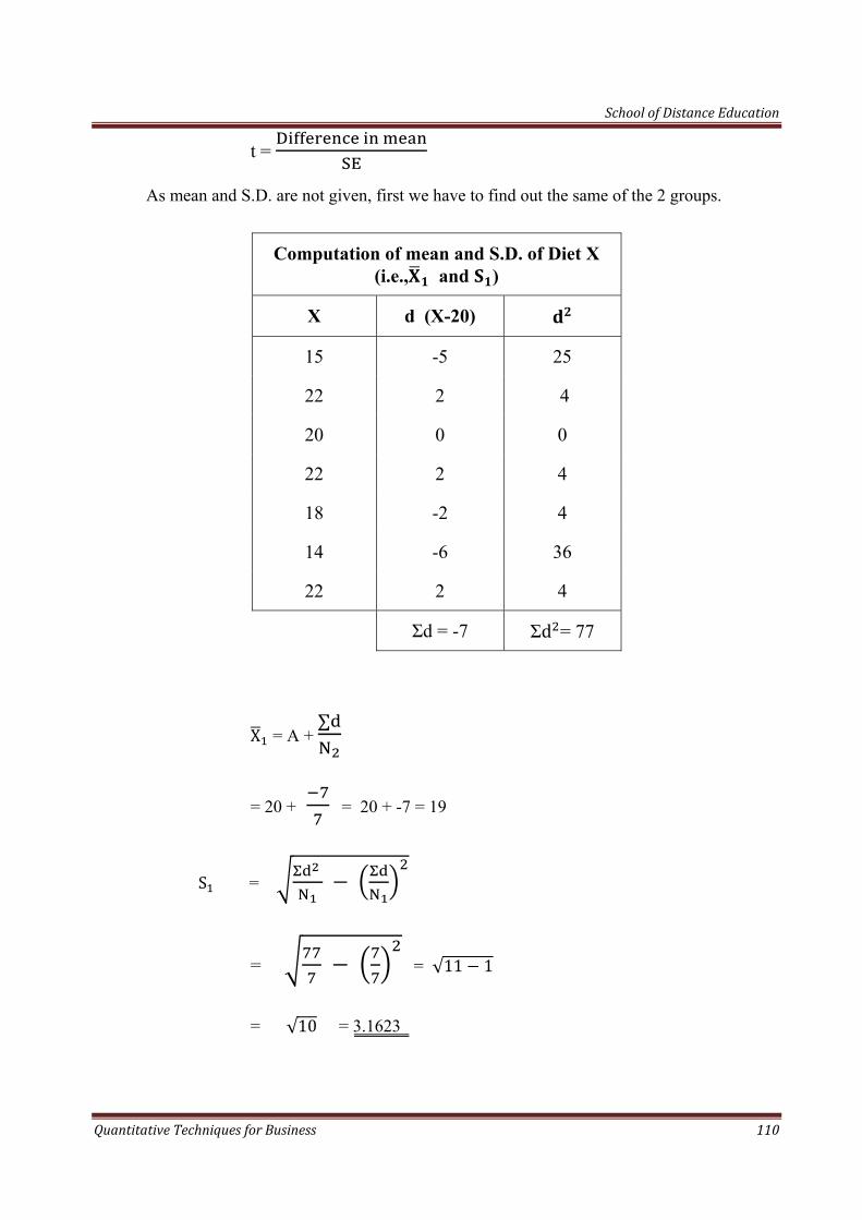
School of Distance Education
Quantitative Techniques for Business 110
t =
As mean and S.D. are not given, first we have to find out the same of the 2 groups.
Computation of mean and S.D. of Diet X (i.e., and )
X d (X-20)
15 -5 25
22 2 4
20 0 0
22 2 4
18 -2 4
14 -6 36
22 2 4
Σd = -7 Σd = 77
X = A + ∑
= 20 + = 20 + -7 = 19
S =
= = √11 1
= √10 = 3.1623

School of Distance Education
Quantitative Techniques for Business 111
Computation of mean and S.D. of Diet X (i.e., and )
X d (X-20)
14 -6 36
24 4 8
12 -8 64
20 0 0
32 12 144
21 1 1
30 10 100
20 0 0
22 2 4
25 5 25
Σd = 20 Σd = 390
X = A + ∑
= 20 + = 20 + 2 = 22
S =
= = √39 4
= √35 = 5.9161
S.E. =
= . .
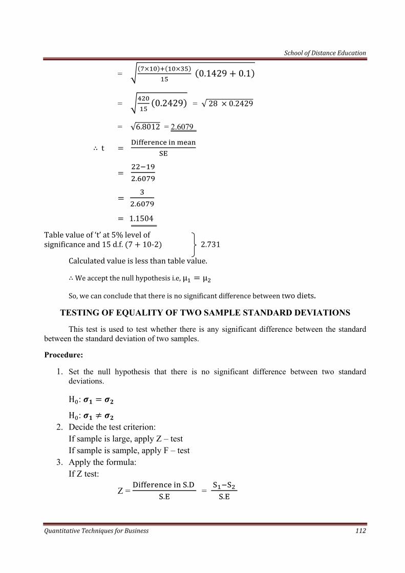
School of Distance Education
Quantitative Techniques for Business 112
= 0.1429 0.1
= 0.2429 = √ 28 0.2429
= √6.8012 = 2.6079
t
.
.
1.1504
Table value of ‘t’ at 5% level of significance and 15 d.f. 7 10‐2 2.731
Calculated value is less than table value.
We accept the null hypothesis i.e, µ µ
So, we can conclude that there is no significant difference between two diets.
TESTING OF EQUALITY OF TWO SAMPLE STANDARD DEVIATIONS
This test is used to test whether there is any significant difference between the standard between the standard deviation of two samples.
Procedure:
1. Set the null hypothesis that there is no significant difference between two standard deviations.
H :
H : 2. Decide the test criterion:
If sample is large, apply Z – test If sample is sample, apply F – test
3. Apply the formula: If Z test:
Z = .
. =
.

School of Distance Education
Quantitative Techniques for Business 113
SE = (When population S.D. are known)
SE = (When population S.D. are not known)
If F – test:
F =
4. Fix the degree of freedom
For Z – test: Infinity
For F – test: n 1, n 1
5. Obtain the table value.
6. Decide whether to accept or reject the null hypothesis.
Qn: A sample of 60 items has S.D of 5 and another sample of 80 items has S.D of 4.5. Can you assert that the two samples belong to the same population?
Sol: H :
H :
Since samples are large, apply Z - test.
Z = .
.
SE =
= . = .
= √0.2083 0.1266 = √0.3349
= 0.5787
Z = ..
= ..
= 0.8640
(Larger value must be numerator and smaller must be denominator)
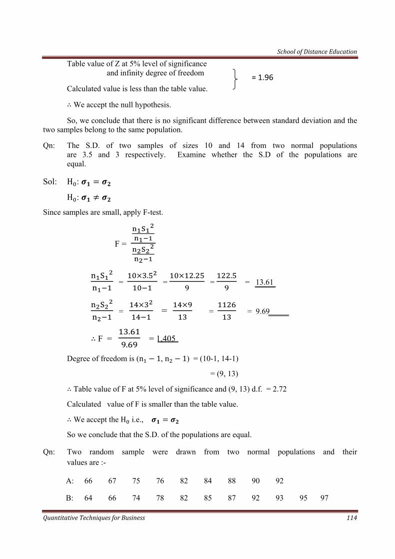
School of Distance Education
Quantitative Techniques for Business 114
Table value of Z at 5% level of significance and infinity degree of freedom
Calculated value is less than the table value.
We accept the null hypothesis.
So, we conclude that there is no significant difference between standard deviation and the two samples belong to the same population.
Qn: The S.D. of two samples of sizes 10 and 14 from two normal populations are 3.5 and 3 respectively. Examine whether the S.D of the populations are equal.
Sol: H :
H :
Since samples are small, apply F-test.
F =
= . =
. = . = 13.61
= = = = 9.69
F = ..
= 1,405
Degree of freedom is (n 1, n 1) = (10-1, 14-1)
= (9, 13)
Table value of F at 5% level of significance and (9, 13) d.f. = 2.72
Calculated value of F is smaller than the table value.
We accept the H i.e.,
So we conclude that the S.D. of the populations are equal.
Qn: Two random sample were drawn from two normal populations and their values are :-
A: 66 67 75 76 82 84 88 90 92
B: 64 66 74 78 82 85 87 92 93 95 97
= 1.96
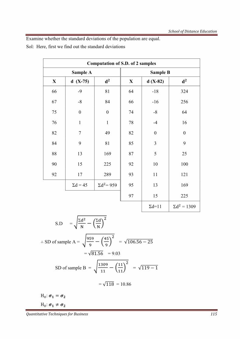
School of Distance Education
Quantitative Techniques for Business 115
Examine whether the standard deviations of the population are equal.
Sol: Here, first we find out the standard deviations
Computation of S.D. of 2 samples
Sample A Sample B
X d (X-75) X d (X-82)
66 -9 81 64 -18 324
67 -8 84 66 -16 256
75 0 0 74 -8 64
76 1 1 78 -4 16
82 7 49 82 0 0
84 9 81 85 3 9
88 13 169 87 5 25
90 15 225 92 10 100
92 17 289 93 11 121
Σd = 45 Σd = 959 95 13 169
97 15 225
Σd=11 Σd = 1309
S.D = Σ Σ
SD of sample A = = √106.56 25
= √81.56 = 9.03
SD of sample B = = √119 1
= √118 = 10.86
H :
H :
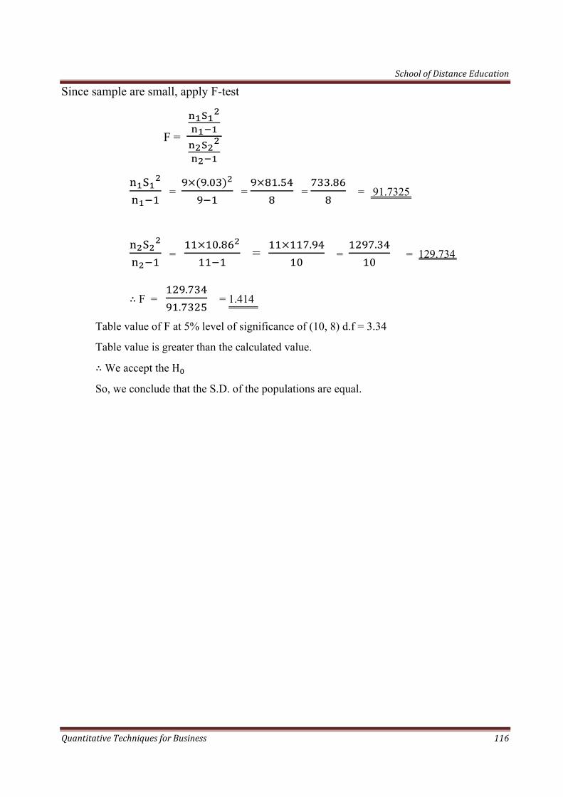
School of Distance Education
Quantitative Techniques for Business 116
Since sample are small, apply F-test
F =
= . =
. = . = 91.7325
= . = . =
. = 129.734
F = ..
= 1.414
Table value of F at 5% level of significance of (10, 8) d.f = 3.34
Table value is greater than the calculated value.
We accept the H
So, we conclude that the S.D. of the populations are equal.

School of Distance Education
Quantitative Techniques for Business 117
CHAPTER 10
NON-PARAMETRIC TESTS
A non-parametric test is a test which is not concerned with testing of parameters. Non-parametric tests do not make any assumption regarding the form of the population. Therefore, non-parametric tests are also called distribution free tests.
Following are the important non-parametric tests:-
1. Chi-square test χ
2. Sign test
3. Signed rank test (Wilcoxon matched pairs test)
4. Rank sum test (Mann-whitney U-test and Kruskal-Wallis H test)
5. Run test
6. Kolmogrov-Smirnor Test (K-S-test)
CHI-SQUARE TEST
The value of chi-square describes the magnitude of difference between observed frequencies and expected frequencies under certain assumptions. χ value (χ quantity) ranges from zero to infinity. It is zero when the expected frequencies and observed frequencies completely coincide. So greater the value of χ , greater is the discrepancy between observed and expected frequencies.
χ -test is a statistical test which tests the significance of difference between observed frequencies and corresponding theoretical frequencies of a distribution without any assumption about the distribution of the population. This is one of the simplest and most widely used non-parametric test in statistical work. This test was developed by Prof. Karl Pearson in 1990.
Uses of - test
The uses of chi-square test are:-
1. Useful for the test of goodness of fit:- χ - test can be used to test whether there is goodness of fit between the observed frequencies and expected frequencies.
2. Useful for the test of independence of attributes:- χ test can be used to test whether two attributes are associated or not.
3. Useful for the test of homogeneity:- χ -test is very useful t5o test whether two attributes are homogeneous or not.
4. Useful for testing given population variance:- χ -test can be used for testing whether the given population variance is acceptable on the basis of samples drawn from that population.

School of Distance Education
Quantitative Techniques for Business 118
-test as a test of goodness of fit:
As a non-parametric test, χ -test is mainly used to test the goodness of fit between the observed frequencies and expected frequencies.
Procedure:-
1. Set up mull hypothesis that there is goodness of fit between observed and expected frequencies.
2. Find the χ value using the following formula:-
χ = Σ
Where O = Observed frequencies
E = Expected frequencies
3. Compute the degree of freedom.
d. f. = n – r – 1
Where ‘r’ is the number of independent constraints to be satisfied by the frequencies
4. Obtain the table value corresponding to the lord of significance and degrees of freedom.
5. Decide whether to accept or reject the null hypothesis. If the calculated value is less than the table value, we accept the null hypothesis and conclude that there is goodness of fit. If the calculated value is more than the table value we reject the null hypothesis and conclude that there is no goodness of fit.
Qn:- A sample analysis of examination result of 200 students were made. It was found that 46 students had failed, 68 secured IIIrd class, 62 IInd class and the rest were placed in the Ist class. Are these figures commensurate with the general examination results which is in the ratio of 2 : 3: 3: 2 for various categories respectively?
Sol: H : The figures commensurate with the general examination results.
H : The figures do not commensurate with the general examination results.
χ = Σ
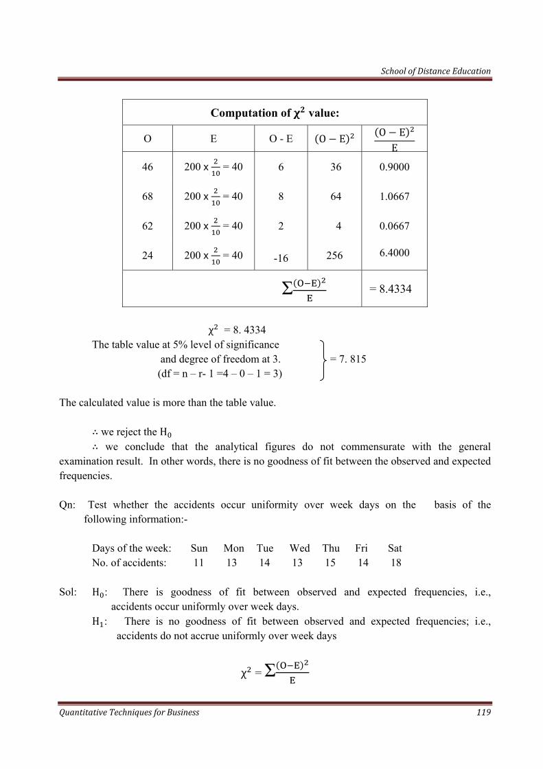
School of Distance Education
Quantitative Techniques for Business 119
Computation of value:
O E O - E O E O EE
46 200 = 40 6 36 0.9000
68 200 = 40 8 64 1.0667
62 200 = 40 2 4 0.0667
24 200 = 40 -16 256 6.4000
Σ = 8.4334
χ = 8. 4334 The table value at 5% level of significance and degree of freedom at 3. = 7. 815 (df = n – r- 1 =4 – 0 – 1 = 3) The calculated value is more than the table value. we reject the H we conclude that the analytical figures do not commensurate with the general examination result. In other words, there is no goodness of fit between the observed and expected frequencies. Qn: Test whether the accidents occur uniformity over week days on the basis of the following information:- Days of the week: Sun Mon Tue Wed Thu Fri Sat No. of accidents: 11 13 14 13 15 14 18 Sol: H : There is goodness of fit between observed and expected frequencies, i.e., accidents occur uniformly over week days. H : There is no goodness of fit between observed and expected frequencies; i.e., accidents do not accrue uniformly over week days
χ = Σ
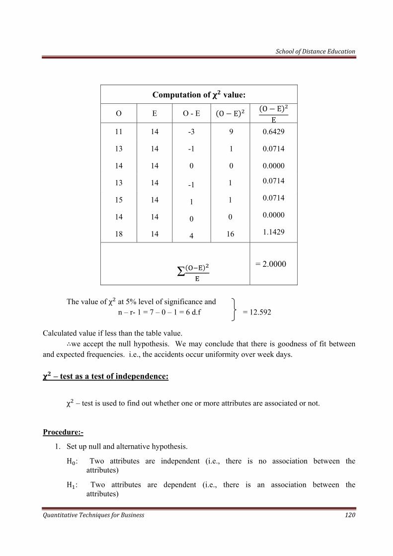
School of Distance Education
Quantitative Techniques for Business 120
Computation of value:
O E O - E O E O EE
11 14 -3 9 0.6429
13 14 -1 1 0.0714
14 14 0 0 0.0000
13 14 -1 1 0.0714
15 14 1 1 0.0714
14 14 0 0 0.0000
18 14 4 16 1.1429
Σ
= 2.0000
The value of χ at 5% level of significance and n – r- 1 = 7 – 0 – 1 = 6 d.f = 12.592 Calculated value if less than the table value. we accept the null hypothesis. We may conclude that there is goodness of fit between and expected frequencies. i.e., the accidents occur uniformity over week days.
– test as a test of independence:
χ – test is used to find out whether one or more attributes are associated or not.
Procedure:-
1. Set up null and alternative hypothesis.
H : Two attributes are independent (i.e., there is no association between the attributes)
H : Two attributes are dependent (i.e., there is an association between the attributes)
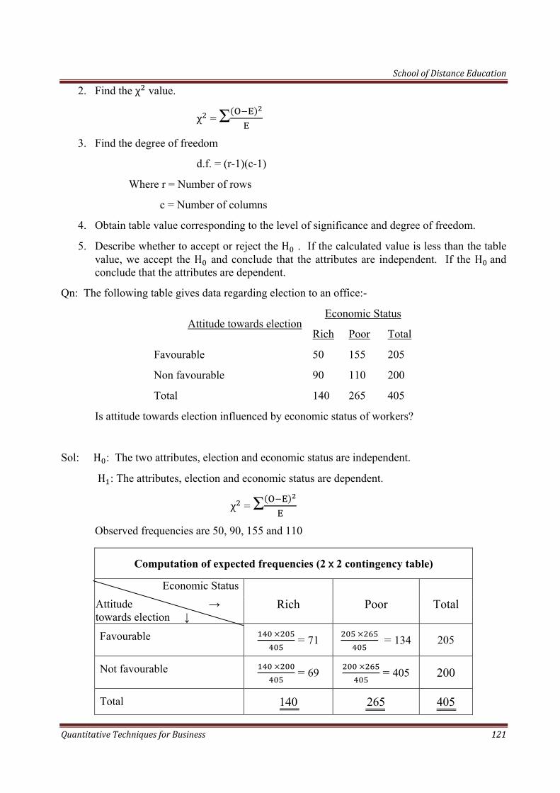
School of Distance Education
Quantitative Techniques for Business 121
2. Find the χ value.
χ = Σ
3. Find the degree of freedom
d.f. = (r-1)(c-1)
Where r = Number of rows
c = Number of columns
4. Obtain table value corresponding to the level of significance and degree of freedom.
5. Describe whether to accept or reject the H . If the calculated value is less than the table value, we accept the H and conclude that the attributes are independent. If the H and conclude that the attributes are dependent.
Qn: The following table gives data regarding election to an office:-
Attitude towards election Economic Status
Rich Poor Total
Favourable 50 155 205
Non favourable 90 110 200
Total 140 265 405
Is attitude towards election influenced by economic status of workers?
Sol: H : The two attributes, election and economic status are independent.
H : The attributes, election and economic status are dependent.
χ = Σ
Observed frequencies are 50, 90, 155 and 110
Computation of expected frequencies (2 2 contingency table)
Economic Status
Rich Poor Total Attitude → towards election ↓
Favourable = 71 = 134 205
Not favourable = 69 = 405 200
Total 140 265 405
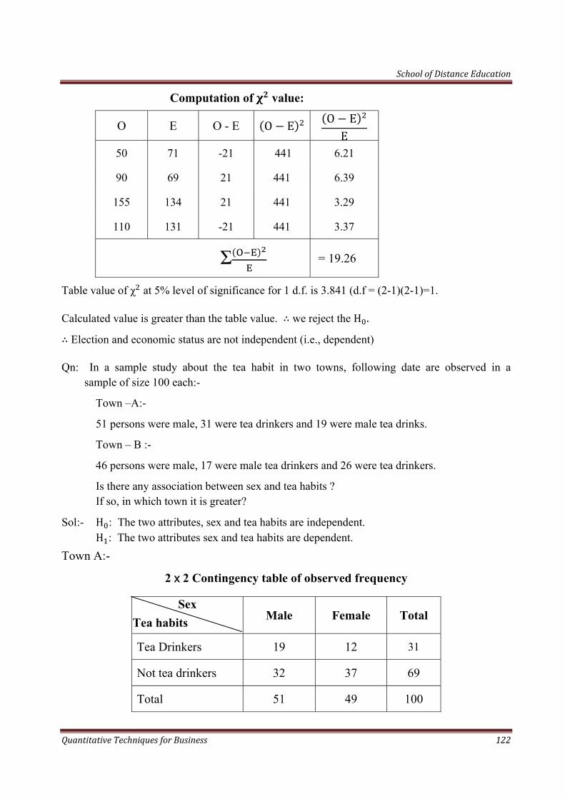
School of Distance Education
Quantitative Techniques for Business 122
Computation of value:
O E O - E O E O EE
50 71 -21 441 6.21
90 69 21 441 6.39
155 134 21 441 3.29
110 131 -21 441 3.37
Σ = 19.26
Table value of χ at 5% level of significance for 1 d.f. is 3.841 (d.f = (2-1)(2-1)=1.
Calculated value is greater than the table value. we reject the H .
Election and economic status are not independent (i.e., dependent)
Qn: In a sample study about the tea habit in two towns, following date are observed in a sample of size 100 each:-
Town –A:-
51 persons were male, 31 were tea drinkers and 19 were male tea drinks.
Town – B :-
46 persons were male, 17 were male tea drinkers and 26 were tea drinkers.
Is there any association between sex and tea habits ? If so, in which town it is greater?
Sol:- H : The two attributes, sex and tea habits are independent. H : The two attributes sex and tea habits are dependent.
Town A:-
2 2 Contingency table of observed frequency
Sex Male Female Total Tea habits
Tea Drinkers 19 12 31
Not tea drinkers 32 37 69
Total 51 49 100
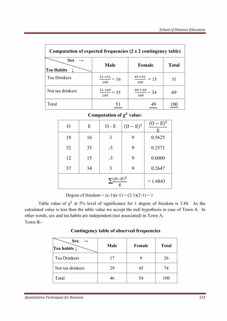
School of Distance Education
Quantitative Techniques for Business 123
Computation of value:
O E O - E O E O EE
19 16 3 9 0.5625
32 35 -3 9 0.2571
12 15 -3 9 0.6000
37 34 3 9 0.2647
Σ = 1.6843
Degree of freedom = (c-1)(r-1) = (2-1)(2-1) = 1
Table value of χ at 5% level of significance for 1 degree of freedom is 3.84. As the calculated value is less than the table value we accept the null hypothesis in case of Town A. In other words, sex and tea habits are independent (not associated) in Town A.
Town B:-
Contingency table of observed frequencies
Sex → Male Female Total Tea habits ↓
Tea Drinkers 17 9 26
Not tea drinkers 29 45 74
Total 46 54 100
Computation of expected frequencies (2 2 contingency table)
Sex → Male Female Total
Tea Habits ↓
Tea Drinkers = 16 = 15 31
Not tea drinkers = 35 = 34 69
Total 51 49 100
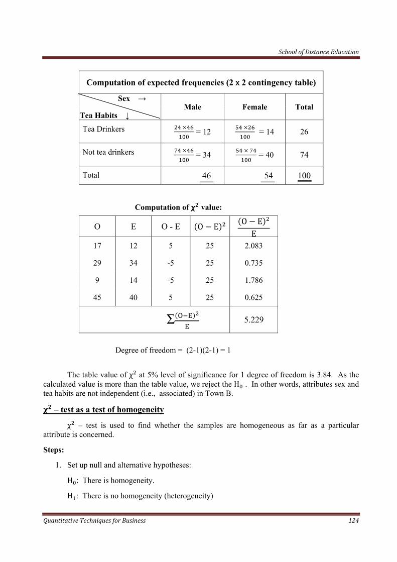
School of Distance Education
Quantitative Techniques for Business 124
Computation of expected frequencies (2 2 contingency table)
Sex → Male Female Total
Tea Habits ↓
Tea Drinkers = 12 = 14 26
Not tea drinkers = 34 = 40 74
Total 46 54 100
Computation of value:
O E O - E O E O EE
17 12 5 25 2.083
29 34 -5 25 0.735
9 14 -5 25 1.786
45 40 5 25 0.625
Σ 5.229
Degree of freedom = (2-1)(2-1) = 1
The table value of χ at 5% level of significance for 1 degree of freedom is 3.84. As the calculated value is more than the table value, we reject the H . In other words, attributes sex and tea habits are not independent (i.e., associated) in Town B.
– test as a test of homogeneity
χ – test is used to find whether the samples are homogeneous as far as a particular attribute is concerned.
Steps:
1. Set up null and alternative hypotheses:
H : There is homogeneity.
H : There is no homogeneity (heterogeneity)
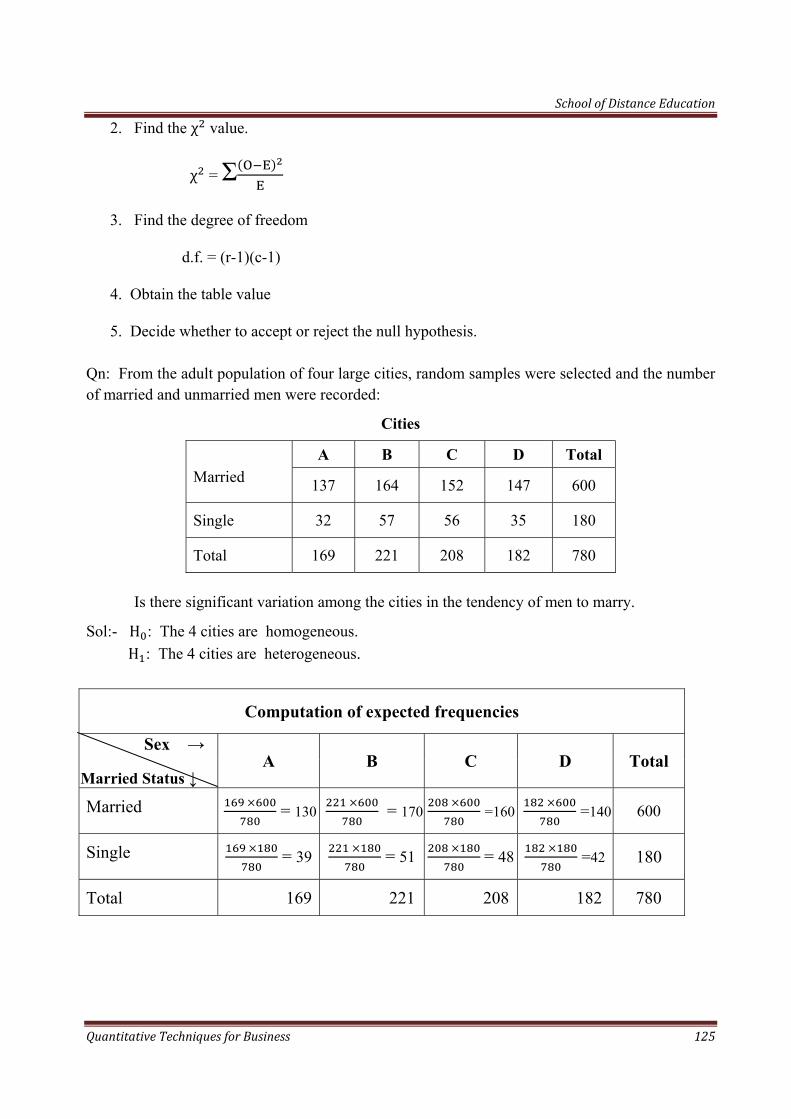
School of Distance Education
Quantitative Techniques for Business 125
2. Find the χ value.
χ = Σ
3. Find the degree of freedom
d.f. = (r-1)(c-1)
4. Obtain the table value
5. Decide whether to accept or reject the null hypothesis. Qn: From the adult population of four large cities, random samples were selected and the number of married and unmarried men were recorded:
Cities
Married
A B C D Total
137 164 152 147 600
Single 32 57 56 35 180
Total 169 221 208 182 780 Is there significant variation among the cities in the tendency of men to marry.
Sol:- H : The 4 cities are homogeneous. H : The 4 cities are heterogeneous.
Computation of expected frequencies
Sex → A B C D Total
Married Status ↓
Married = 130 = 170 =160 =140 600
Single = 39 = 51 = 48 =42 180
Total 169 221 208 182 780
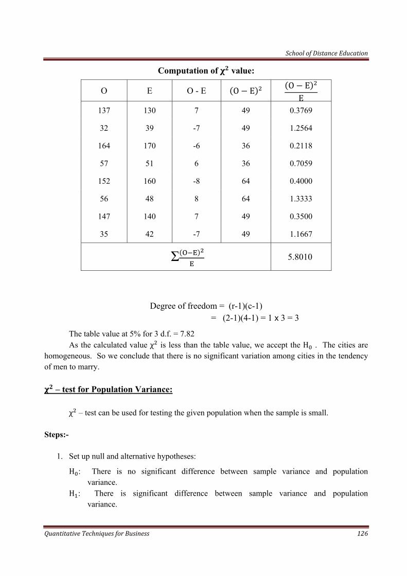
School of Distance Education
Quantitative Techniques for Business 126
Computation of value:
O E O - E O E O EE
137 130 7 49 0.3769
32 39 -7 49 1.2564
164 170 -6 36 0.2118
57 51 6 36 0.7059
152 160 -8 64 0.4000
56 48 8 64 1.3333
147 140 7 49 0.3500
35 42 -7 49 1.1667
Σ 5.8010
Degree of freedom = (r-1)(c-1) = (2-1)(4-1) = 1 3 = 3
The table value at 5% for 3 d.f. = 7.82 As the calculated value χ is less than the table value, we accept the H . The cities are homogeneous. So we conclude that there is no significant variation among cities in the tendency of men to marry.
– test for Population Variance: χ – test can be used for testing the given population when the sample is small. Steps:-
1. Set up null and alternative hypotheses:
H : There is no significant difference between sample variance and population variance.
H : There is significant difference between sample variance and population variance.

School of Distance Education
Quantitative Techniques for Business 127
2. Find the χ value.
χ = Where = Sample variance = Population variance
3. Find the degree of freedom d.f. = n-1
4. Obtain the table value
5. Decide whether to accept or reject the null hypothesis
Qn: The standard deviation of a sample of 10 observations from a normal population was formed to be 5. Examine whether this is consistent with the hypothesis that the standard deviation of the population is 5.3.
Sol: H : There is no significant difference between sample standard deviation and population standard deviation.
H : There is significant difference between sample standard deviation and population standard deviation.
χ = = .
= .
= 8.8999
Table value of χ at 5% level of significance of 9 d.f. = 16.9 calculated value of χ is less than the table value , we accept in null hypothesis. So we conclude that there is no significant difference between sample variance and population variance.
Limitations of Chi-square tests:-
1. It is not as reliable as a parametric test. Hence it should be used only when parametric tests cannot be used.
2. χ value can not be computed when the given values are proportions or percentages.
WILCOXON MATCHED PAIRS TEST
SIGNED RANK TEST
Signed rank test was developed by Frank Wilcoxon. It is an important non-parametric test. This method is used when we can determine both direction and magnitude of difference between matched values.
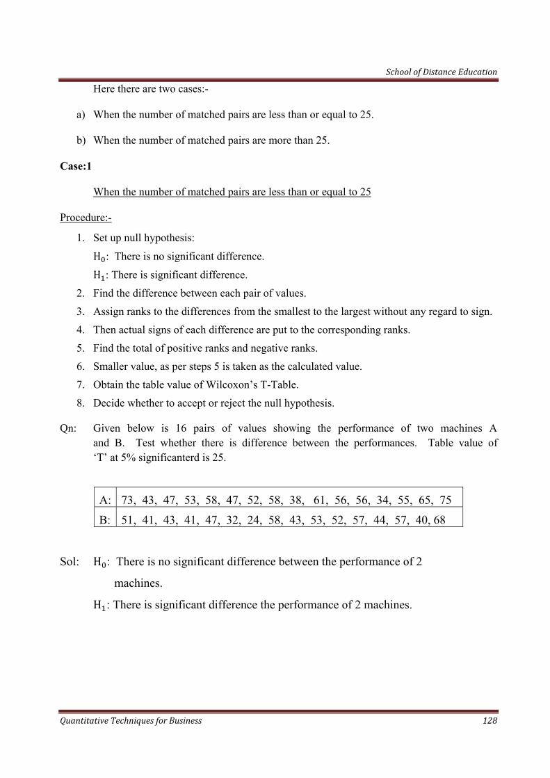
School of Distance Education
Quantitative Techniques for Business 128
Here there are two cases:-
a) When the number of matched pairs are less than or equal to 25.
b) When the number of matched pairs are more than 25.
Case:1
When the number of matched pairs are less than or equal to 25
Procedure:-
1. Set up null hypothesis:
H : There is no significant difference.
H : There is significant difference.
2. Find the difference between each pair of values.
3. Assign ranks to the differences from the smallest to the largest without any regard to sign.
4. Then actual signs of each difference are put to the corresponding ranks.
5. Find the total of positive ranks and negative ranks.
6. Smaller value, as per steps 5 is taken as the calculated value.
7. Obtain the table value of Wilcoxon’s T-Table.
8. Decide whether to accept or reject the null hypothesis.
Qn: Given below is 16 pairs of values showing the performance of two machines A and B. Test whether there is difference between the performances. Table value of ‘T’ at 5% significanterd is 25.
A: 73, 43, 47, 53, 58, 47, 52, 58, 38, 61, 56, 56, 34, 55, 65, 75
B: 51, 41, 43, 41, 47, 32, 24, 58, 43, 53, 52, 57, 44, 57, 40, 68
Sol: H : There is no significant difference between the performance of 2
machines.
H : There is significant difference the performance of 2 machines.
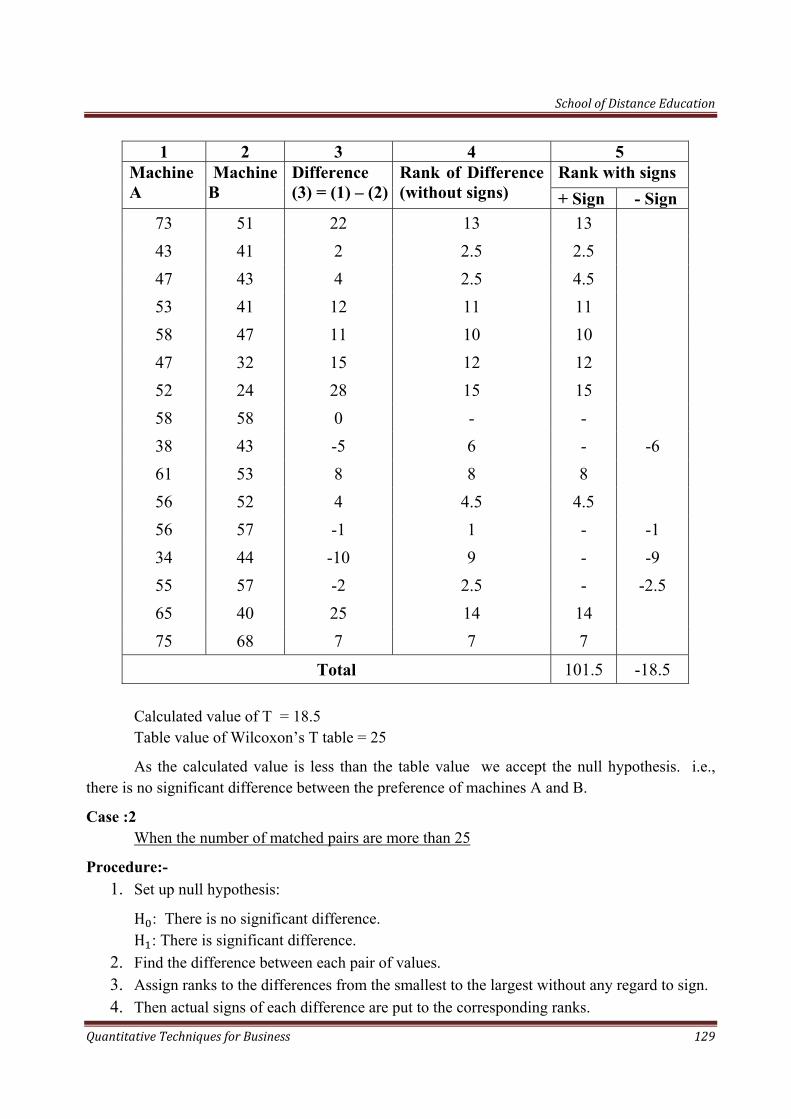
School of Distance Education
Quantitative Techniques for Business 129
1 2 3 4 5
Machine A
Machine B
Difference (3) = (1) – (2)
Rank of Difference (without signs)
Rank with signs + Sign - Sign
73 51 22 13 13 43 41 2 2.5 2.5 47 43 4 2.5 4.5 53 41 12 11 11 58 47 11 10 10 47 32 15 12 12 52 24 28 15 15 58 58 0 - - 38 43 -5 6 - -6 61 53 8 8 8 56 52 4 4.5 4.5 56 57 -1 1 - -1 34 44 -10 9 - -9 55 57 -2 2.5 - -2.5 65 40 25 14 14 75 68 7 7 7
Total 101.5 -18.5 Calculated value of T = 18.5 Table value of Wilcoxon’s T table = 25
As the calculated value is less than the table value we accept the null hypothesis. i.e., there is no significant difference between the preference of machines A and B.
Case :2 When the number of matched pairs are more than 25
Procedure:- 1. Set up null hypothesis:
H : There is no significant difference. H : There is significant difference.
2. Find the difference between each pair of values. 3. Assign ranks to the differences from the smallest to the largest without any regard to sign. 4. Then actual signs of each difference are put to the corresponding ranks.
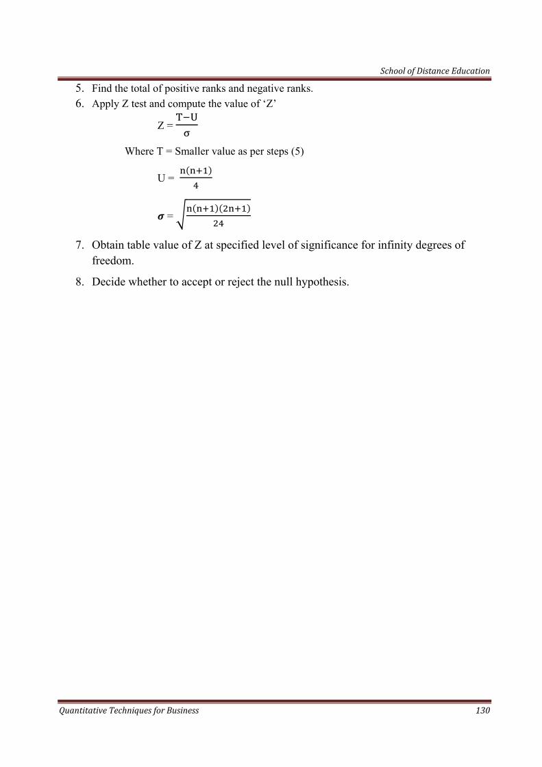
School of Distance Education
Quantitative Techniques for Business 130
5. Find the total of positive ranks and negative ranks. 6. Apply Z test and compute the value of ‘Z’
Z =
Where T = Smaller value as per steps (5)
U =
=
7. Obtain table value of Z at specified level of significance for infinity degrees of freedom.
8. Decide whether to accept or reject the null hypothesis.
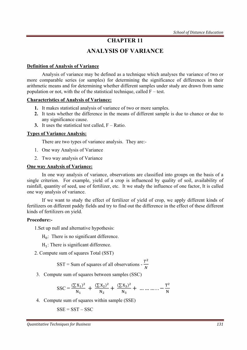
School of Distance Education
Quantitative Techniques for Business 131
CHAPTER 11
ANALYSIS OF VARIANCE
Definition of Analysis of Variance Analysis of variance may be defined as a technique which analyses the variance of two or more comparable series (or samples) for determining the significance of differences in their arithmetic means and for determining whether different samples under study are drawn from same population or not, with the of the statistical technique, called F – test.
Characteristics of Analysis of Variance: 1. It makes statistical analysis of variance of two or more samples. 2. It tests whether the difference in the means of different sample is due to chance or due to
any significance cause. 3. It uses the statistical test called, F – Ratio.
Types of Variance Analysis: There are two types of variance analysis. They are:-
1. One way Analysis of Variance
2. Two way analysis of Variance
One way Analysis of Variance: In one way analysis of variance, observations are classified into groups on the basis of a single criterion. For example, yield of a crop is influenced by quality of soil, availability of rainfall, quantity of seed, use of fertilizer, etc. It we study the influence of one factor, It is called one way analysis of variance.
If we want to study the effect of fertilizer of yield of crop, we apply different kinds of fertilizers on different paddy fields and try to find out the difference in the effect of these different kinds of fertilizers on yield.
Procedure:- 1.Set up null and alternative hypothesis:
H : There is no significant difference.
H : There is significant difference.
2. Compute sum of squares Total (SST)
SST = Sum of squares of all observations -
3. Compute sum of squares between samples (SSC)
SSC = ∑ ∑ ∑ ……… . .
4. Compute sum of squares within sample (SSE)
SSE = SST – SSC
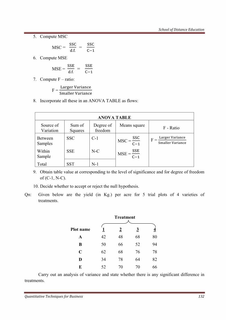
School of Distance Education
Quantitative Techniques for Business 132
5. Compute MSC
MSC = . .
=
6. Compute MSE
MSE = . .
=
7. Compute F – ratio:
F =
8. Incorporate all these in an ANOVA TABLE as flows:
ANOVA TABLE
Source of Variation
Sum of Squares
Degree of freedom
Means square F - Ratio
Between Samples
SSC C-1 MSC = F =
Within Sample
SSE N-C MSE =
Total SST N-1
9. Obtain table value at corresponding to the level of significance and for degree of freedom of (C-1, N-C).
10. Decide whether to accept or reject the null hypothesis.
Qn: Given below are the yield (in Kg.) per acre for 5 trial plots of 4 varieties of treatments.
Treatment
Plot name 1 2 3 4
A 42 48 68 80
B 50 66 52 94
C 62 68 76 78
D 34 78 64 82
E 52 70 70 66
Carry out an analysis of variance and state whether there is any significant difference in treatments.
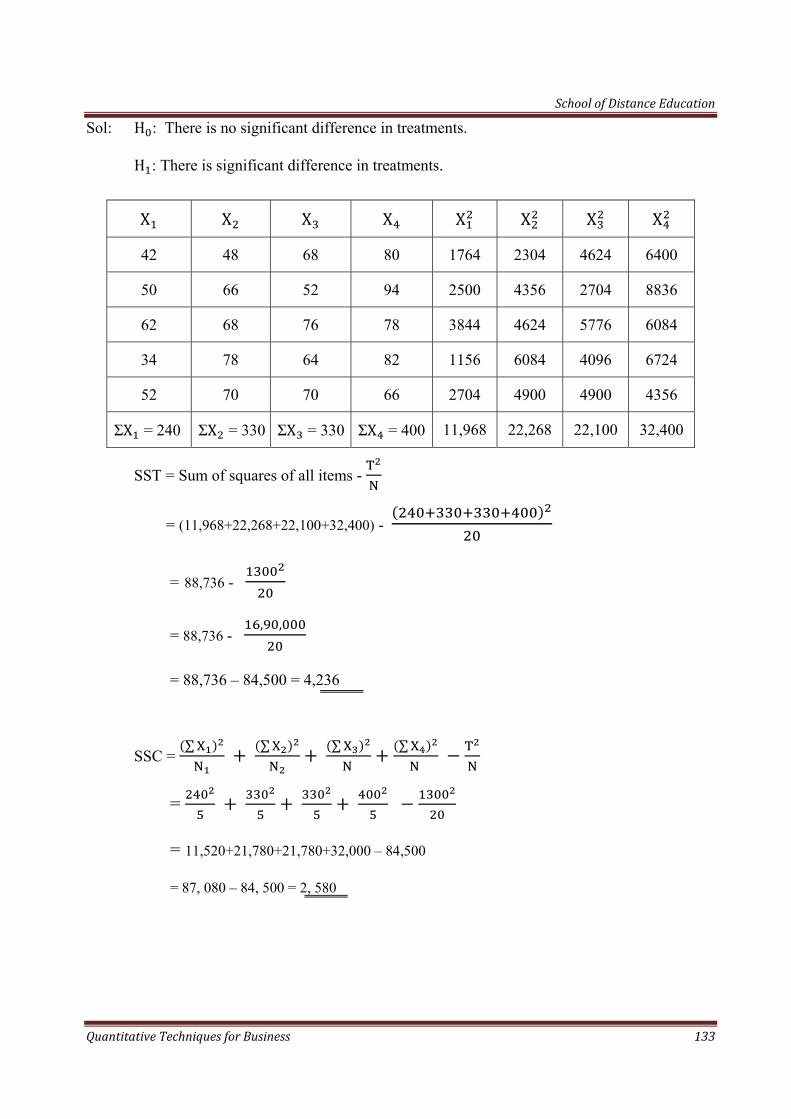
School of Distance Education
Quantitative Techniques for Business 133
Sol: H : There is no significant difference in treatments.
H : There is significant difference in treatments.
X X X X X X X X
42 48 68 80 1764 2304 4624 6400
50 66 52 94 2500 4356 2704 8836
62 68 76 78 3844 4624 5776 6084
34 78 64 82 1156 6084 4096 6724
52 70 70 66 2704 4900 4900 4356
ΣX = 240 ΣX = 330 ΣX = 330 ΣX = 400 11,968 22,268 22,100 32,400
SST = Sum of squares of all items -
= (11,968+22,268+22,100+32,400) -
= 88,736 -
= 88,736 - , ,
= 88,736 – 84,500 = 4,236
SSC = ∑ ∑ ∑
∑
=
= 11,520+21,780+21,780+32,000 – 84,500
= 87, 080 – 84, 500 = 2, 580
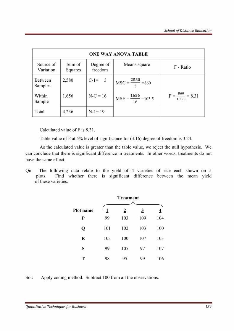
School of Distance Education
Quantitative Techniques for Business 134
ONE WAY ANOVA TABLE
Source of Variation
Sum of Squares
Degree of freedom
Means square F - Ratio
Between Samples
2,580 C-1= 3 MSC = =860
F = .
= 8.31 Within Sample
1,656 N-C = 16 MSE = =103.5
Total 4,236 N-1= 19
Calculated value of F is 8.31.
Table value of F at 5% level of significance for (3.16) degree of freedom is 3.24.
As the calculated value is greater than the table value, we reject the null hypothesis. We can conclude that there is significant difference in treatments. In other words, treatments do not have the same effect.
Qn: The following data relate to the yield of 4 varieties of rice each shown on 5 plots. Find whether there is significant difference between the mean yield of these varieties.
Treatment
Plot name 1 2 3 4
P 99 103 109 104
Q 101 102 103 100
R 103 100 107 103
S 99 105 97 107
T 98 95 99 106
Sol: Apply coding method. Subtract 100 from all the observations.
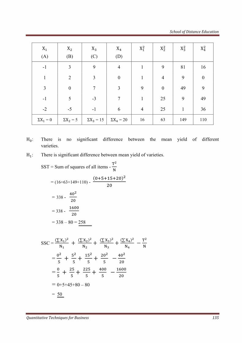
School of Distance Education
Quantitative Techniques for Business 135
X (A)
X (B)
X (C)
X (D)
X
X X X
-1 3 9 4 1 9 81 16
1 2 3 0 1 4 9 0
3 0 7 3 9 0 49 9
-1 5 -3 7 1 25 9 49
-2 -5 -1 6 4 25 1 36
ΣX = 0 ΣX = 5 ΣX = 15 ΣX = 20 16 63 149 110
H : There is no significant difference between the mean yield of different varieties.
H : There is significant difference between mean yield of varieties.
SST = Sum of squares of all items -
= (16+63+149+110) -
= 338 -
= 338 -
= 338 – 80 = 258
SSC = ∑ ∑ ∑ ∑
=
=
= 0+5+45+80 – 80 = 50
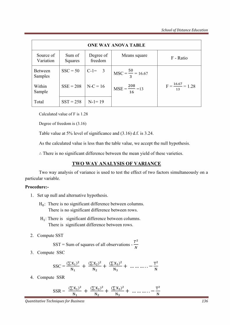
School of Distance Education
Quantitative Techniques for Business 136
ONE WAY ANOVA TABLE
Source of Variation
Sum of Squares
Degree of freedom
Means square F - Ratio
Between Samples
SSC = 50 C-1= 3 MSC = = 16.67
F = . = 1.28 Within Sample
SSE = 208 N-C = 16 MSE = =13
Total SST = 258 N-1= 19
Calculated value of F is 1.28
Degree of freedom is (3.16)
Table value at 5% level of significance and (3.16) d.f. is 3.24.
As the calculated value is less than the table value, we accept the null hypothesis.
There is no significant difference between the mean yield of these varieties.
TWO WAY ANALYSIS OF VARIANCE
Two way analysis of variance is used to test the effect of two factors simultaneously on a particular variable.
Procedure:-
1. Set up null and alternative hypothesis.
H : There is no significant difference between columns. There is no significant difference between rows.
H : There is significant difference between columns. There is significant difference between rows.
2. Compute SST
SST = Sum of squares of all observations -
3. Compute SSC
SSC = ∑ ∑ ∑ ……… . .
4. Compute SSR
SSR = ∑ ∑ ∑ ……… . .
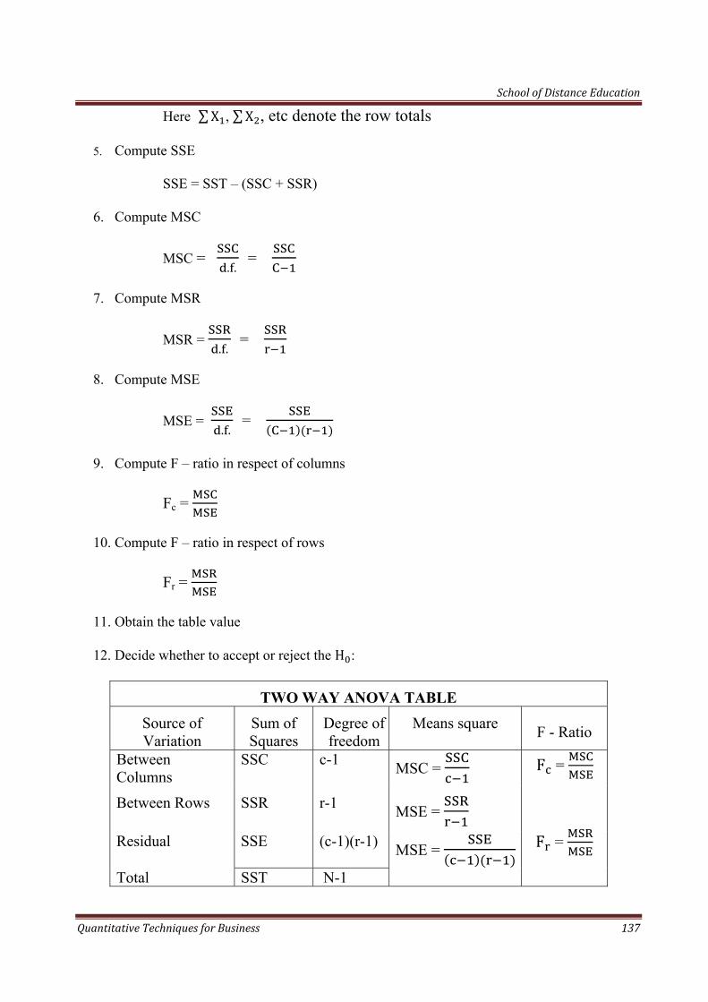
School of Distance Education
Quantitative Techniques for Business 137
Here ∑X , ∑X , etc denote the row totals
5. Compute SSE
SSE = SST – (SSC + SSR)
6. Compute MSC
MSC = . .
=
7. Compute MSR
MSR = . .
=
8. Compute MSE
MSE = . .
=
9. Compute F – ratio in respect of columns
Fc =
10. Compute F – ratio in respect of rows
Fr =
11. Obtain the table value
12. Decide whether to accept or reject the H :
TWO WAY ANOVA TABLE Source of Variation
Sum of Squares
Degree of freedom
Means square F - Ratio
Between Columns
SSC c-1 MSC = F =
F =
Between Rows SSR r-1 MSE = Residual SSE (c-1)(r-1) MSE =
Total SST N-1
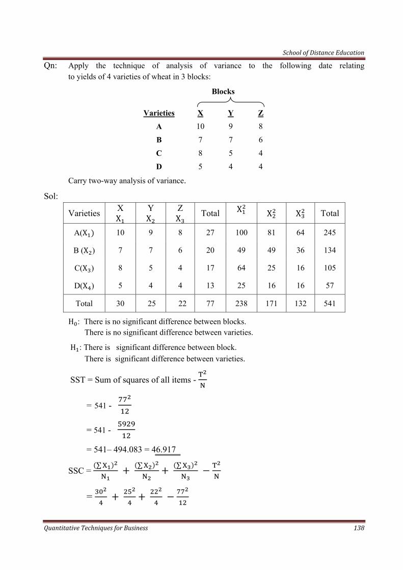
School of Distance Education
Quantitative Techniques for Business 138
Qn: Apply the technique of analysis of variance to the following date relating to yields of 4 varieties of wheat in 3 blocks:
Blocks
Varieties X Y Z
A 10 9 8
B 7 7 6
C 8 5 4
D 5 4 4
Carry two-way analysis of variance.
Sol:
Varieties X X
Y X
Z X Total X
X X Total
A(X 10 9 8 27 100 81 64 245
B (X ) 7 7 6 20 49 49 36 134
C(X ) 8 5 4 17 64 25 16 105
D(X ) 5 4 4 13 25 16 16 57
Total 30 25 22 77 238 171 132 541
H : There is no significant difference between blocks. There is no significant difference between varieties.
H : There is significant difference between block. There is significant difference between varieties.
SST = Sum of squares of all items -
= 541 -
= 541 -
= 541– 494.083 = 46.917
SSC = ∑ ∑ ∑
=

School of Distance Education
Quantitative Techniques for Business 139
=
= 225+156.25+121 – 494.083 = 502.25 – 494.083 = 8.167
SSR = ∑ ∑ ∑ ∑
=
=
= 243+133.333+96.333+56.333 – 494.083 = 34.916
TWO WAY ANOVA TABLE
Source of Variation
Sum of Squares
Degree of freedom
Means square F - Ratio
Between Columns
SSC= 8.167 c-1= 2 MSC = . =4.084 F = ..
= 6.39
F = ..
= 18.21
Between Rows
SSR=34.91 r-1= 3 MSE = . = 11.639
Residual SSE= 3.834 (c-1)(r-1)=6 MSE = . =0.639
Total SST= 46.917 N-1= 11
Between columns (blocks):-
Degree of freedom = (2, 6)
Calculated Value = 6.39
Table Value = 5.1433
As the calculated value is more than the table value, we reject the null hypothesis. It is concluded that there is significant difference between blocks.
i.e., the mean productivity between blocks are not same.
Between rows (varieties):-
Degree of freedom = (3.6)
Calculated value = 18.21
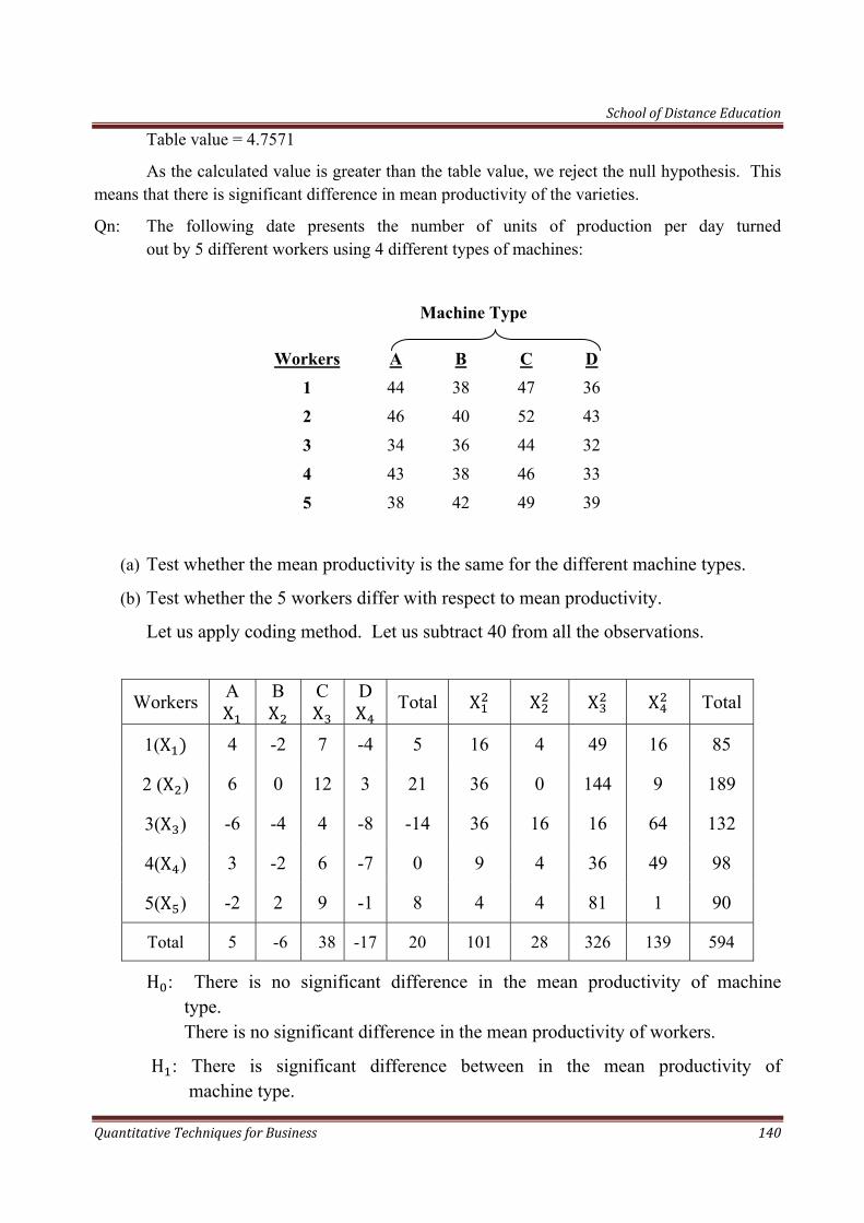
School of Distance Education
Quantitative Techniques for Business 140
Table value = 4.7571
As the calculated value is greater than the table value, we reject the null hypothesis. This means that there is significant difference in mean productivity of the varieties.
Qn: The following date presents the number of units of production per day turned out by 5 different workers using 4 different types of machines:
Machine Type
Workers A B C D
1 44 38 47 36
2 46 40 52 43
3 34 36 44 32
4 43 38 46 33
5 38 42 49 39
(a) Test whether the mean productivity is the same for the different machine types.
(b) Test whether the 5 workers differ with respect to mean productivity.
Let us apply coding method. Let us subtract 40 from all the observations.
Workers A X
B X
C X
D X Total X X X X Total
1(X 4 -2 7 -4 5 16 4 49 16 85
2 (X ) 6 0 12 3 21 36 0 144 9 189
3(X ) -6 -4 4 -8 -14 36 16 16 64 132
4(X ) 3 -2 6 -7 0 9 4 36 49 98
5(X ) -2 2 9 -1 8 4 4 81 1 90
Total 5 -6 38 -17 20 101 28 326 139 594
H : There is no significant difference in the mean productivity of machine type. There is no significant difference in the mean productivity of workers.
H : There is significant difference between in the mean productivity of machine type.
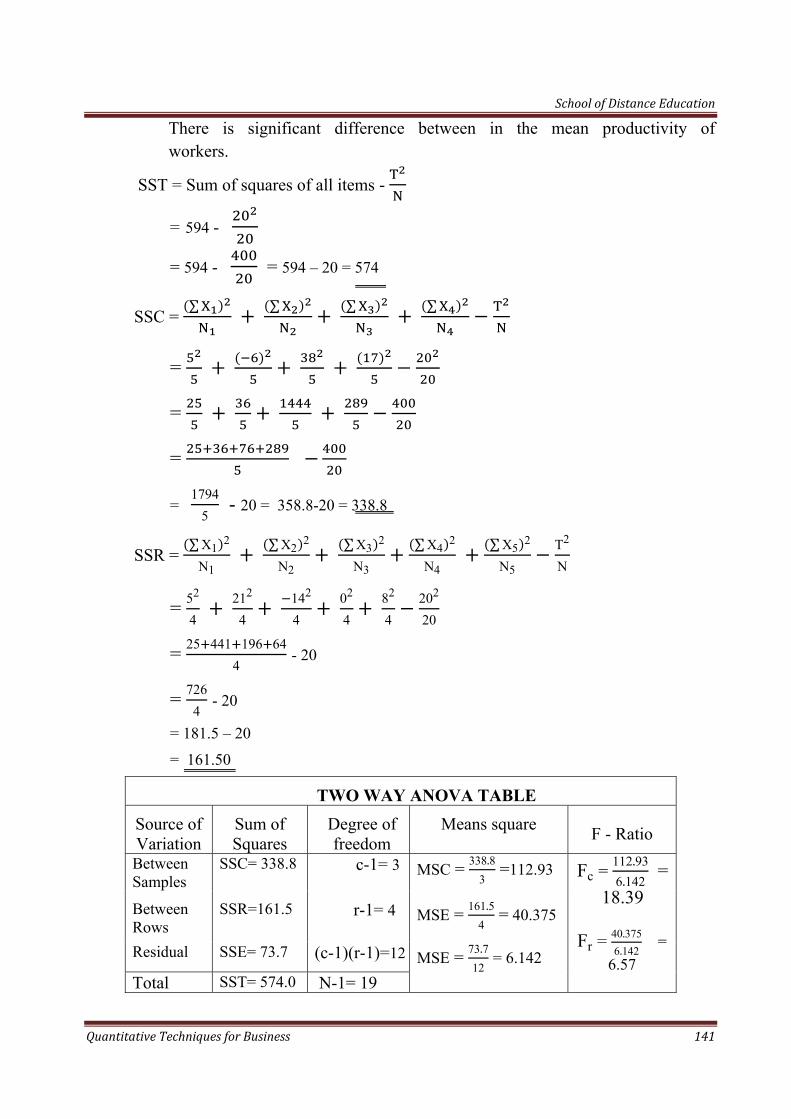
School of Distance Education
Quantitative Techniques for Business 141
There is significant difference between in the mean productivity of workers.
SST = Sum of squares of all items -
= 594 -
= 594 - = 594 – 20 = 574
SSC = ∑ ∑ ∑ ∑
=
=
=
= 1794
5 - 20 = 358.8-20 = 338.8
SSR = ∑X1
2
N1 ∑X2
2
N2 ∑X3
2
N3
∑X42
N4 ∑X5
2
N5
T2
N
= 52
4 212
4 142
4 0
2
4 8
2
4202
20
= 25 441 196 644
- 20
= 7264
- 20
= 181.5 – 20
= 161.50
TWO WAY ANOVA TABLE
Source of Variation
Sum of Squares
Degree of freedom
Means square F - Ratio
Between Samples
SSC= 338.8 c-1= 3 MSC = 338.83
=112.93 Fc = 112.936.142
= 18.39
Fr = 40.375
6.142 =
6.57
Between Rows
SSR=161.5 r-1= 4 MSE = 161.54
= 40.375
Residual SSE= 73.7 (c-1)(r-1)=12 MSE = 73.712
= 6.142 Total SST= 574.0 N-1= 19
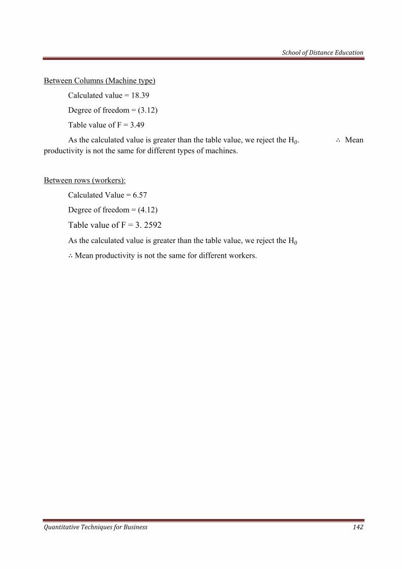
School of Distance Education
Quantitative Techniques for Business 142
Between Columns (Machine type)
Calculated value = 18.39
Degree of freedom = (3.12)
Table value of F = 3.49
As the calculated value is greater than the table value, we reject the H0. Mean productivity is not the same for different types of machines.
Between rows (workers):
Calculated Value = 6.57
Degree of freedom = (4.12)
Table value of F = 3. 2592
As the calculated value is greater than the table value, we reject the H0
Mean productivity is not the same for different workers.