Embed Size (px)
Citation preview
B.Hargreaves - RAD 229
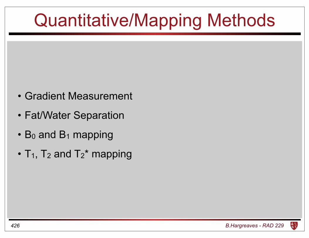
Quantitative/Mapping Methods
• Gradient Measurement
• Fat/Water Separation
• B0 and B1 mapping
• T1, T2 and T2* mapping
426
B.Hargreaves - RAD 229
Gradient Measurement
• Duyn method
• Modifications
427
B.Hargreaves - RAD 229
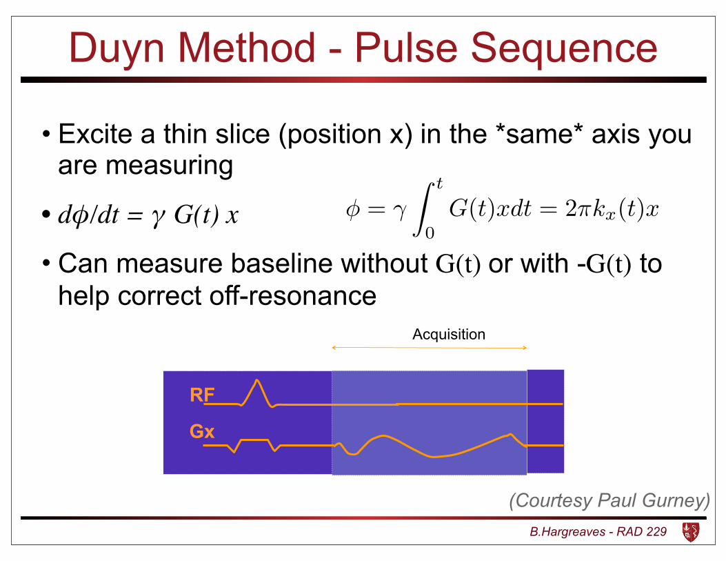
Duyn Method - Pulse Sequence
• Excite a thin slice (position x) in the *same* axis you are measuring
• dφ/dt = γ G(t) x
• Can measure baseline without G(t) or with -G(t) to help correct off-resonance
RF
Gx
Acquisition
(Courtesy Paul Gurney)
� = �
Zt
0G(t)xdt = 2⇡k
x
(t)x
B.Hargreaves - RAD 229
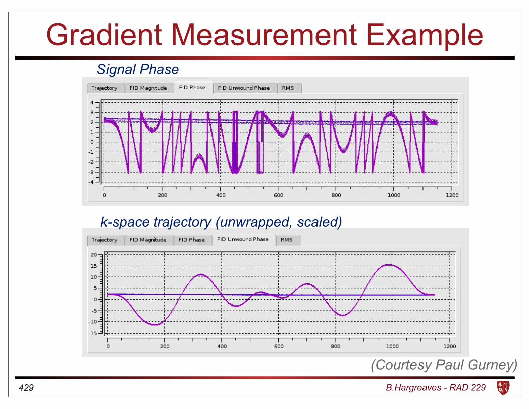
Gradient Measurement Example
429
(Courtesy Paul Gurney)
Signal Phase
k-space trajectory (unwrapped, scaled)
B.Hargreaves - RAD 229
Gradient Measurement
• Can play opposite gradients, excite opposite slices
• Separate different effects:
• off-resonance (independent of gradient)
• eddy currents (linear with gradient G)
• concomitant gradient terms (G2)
B.Hargreaves - RAD 229
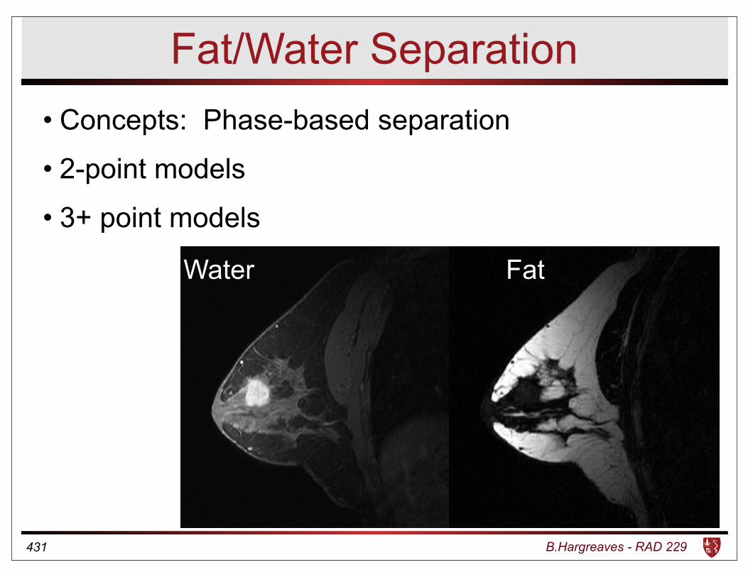
Fat/Water Separation
Water Fat
431
• Concepts: Phase-based separation
• 2-point models
• 3+ point models
B.Hargreaves - RAD 229
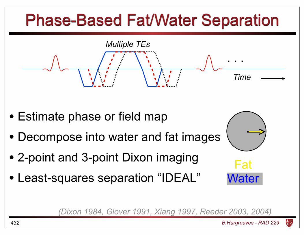
Phase-Based Fat/Water Separation
(Dixon 1984, Glover 1991, Xiang 1997, Reeder 2003, 2004)
Multiple TEs
Time
. . .
• Estimate phase or field map
• Decompose into water and fat images
• 2-point and 3-point Dixon imaging
• Least-squares separation “IDEAL”Fat
Water
432
B.Hargreaves - RAD 229
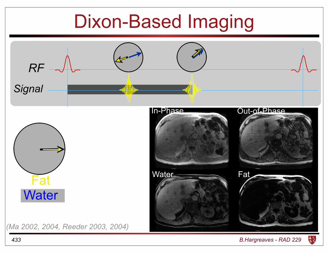
Dixon-Based Imaging
RF
Signal
FatWater
(Ma 2002, 2004, Reeder 2003, 2004)
433
Water Fat
In-Phase Out-of-Phase
B.Hargreaves - RAD 229
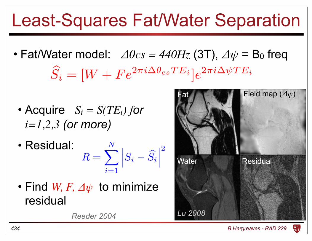
Least-Squares Fat/Water Separation
• Fat/Water model: Δθcs = 440Hz (3T), Δψ = Β0 freq
434
bSi = [W + Fe2⇡i�✓csTEi ]e2⇡i� TEi
R =NX
i=1
���Si � bSi
���2
• Acquire Si = S(TEi) for i=1,2,3 (or more)
• Residual:
• Find W, F, Δψ to minimize residual
Fat
Water Residual
Field map (Δψ)
Reeder 2004 Lu 2008
B.Hargreaves - RAD 229
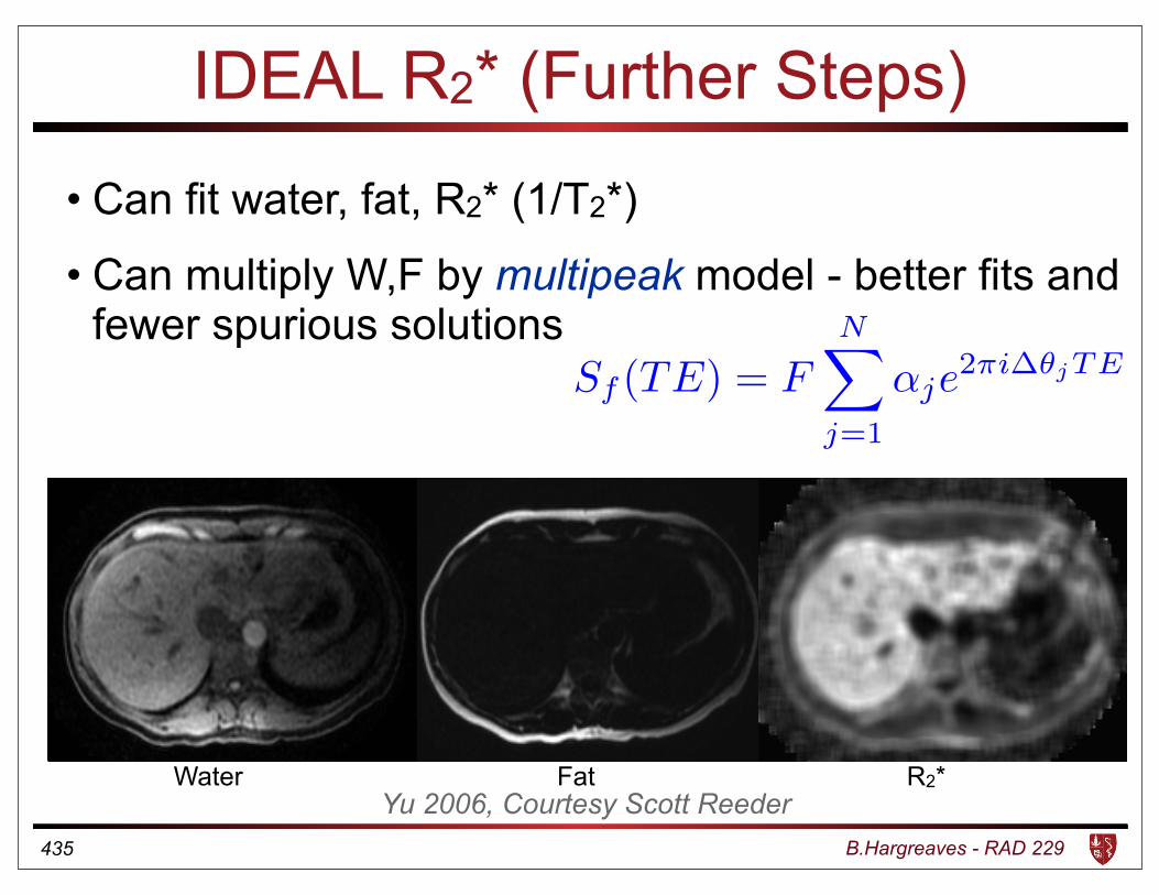
IDEAL R2* (Further Steps)
• Can fit water, fat, R2* (1/T2*)
• Can multiply W,F by multipeak model - better fits and fewer spurious solutions
435
R2*Water FatYu 2006, Courtesy Scott Reeder
Sf (TE) = FNX
j=1
↵je2⇡i�✓jTE
B.Hargreaves - RAD 229
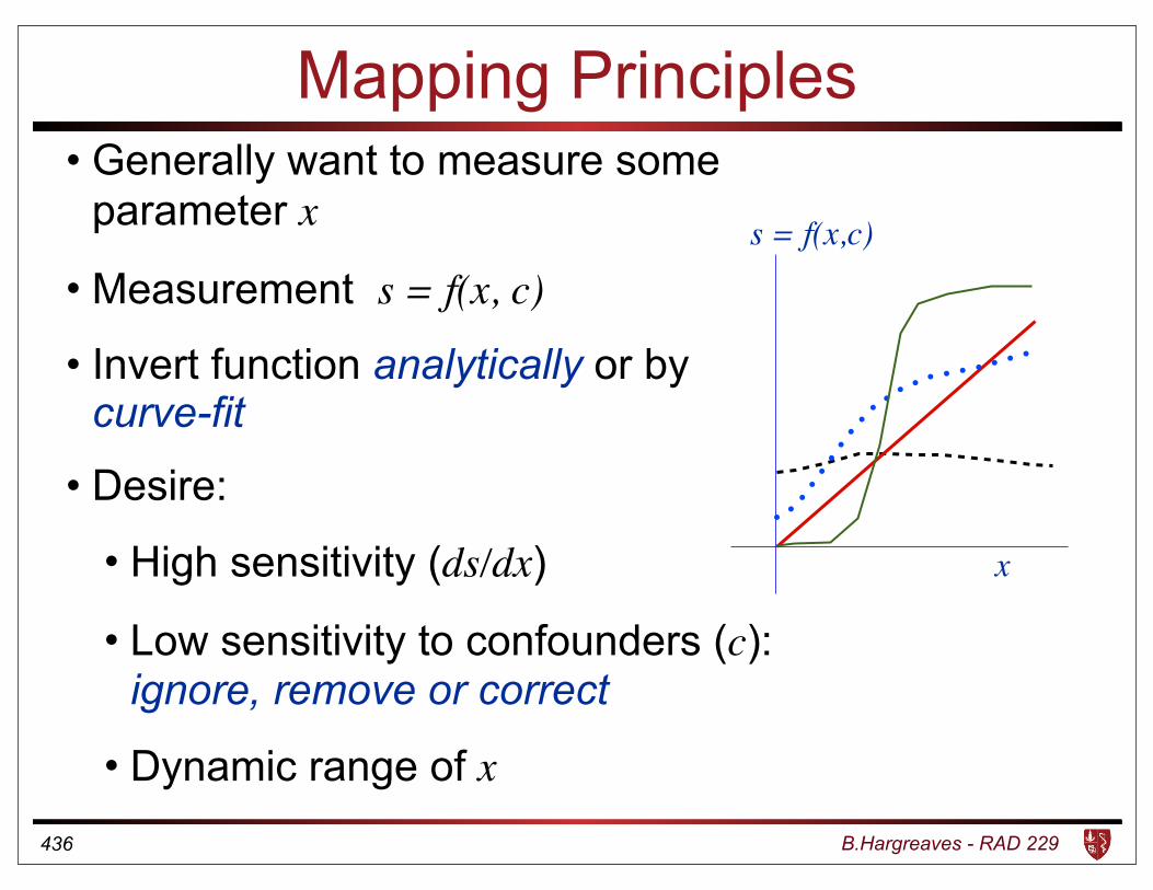
Insensitive
Best? (linear)
Good!
Limited Dynamic Range (x)
Mapping Principles• Generally want to measure some
parameter x
• Measurement s = f(x, c)
• Invert function analytically or by curve-fit
• Desire:
• High sensitivity (ds/dx)
• Low sensitivity to confounders (c): ignore, remove or correct
• Dynamic range of x436
x
s = f(x,c)
B.Hargreaves - RAD 229
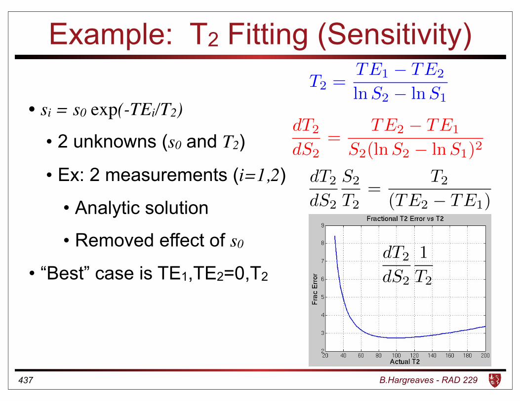
Example: T2 Fitting (Sensitivity)
• si = s0 exp(-TEi/T2)
• 2 unknowns (s0 and T2)
• Ex: 2 measurements (i=1,2)
• Analytic solution
• Removed effect of s0
• “Best” case is TE1,TE2=0,T2
437
T2 =TE1 � TE2
lnS2 � lnS1
dT2
dS2=
TE2 � TE1
S2(lnS2 � lnS1)2
dT2
dS2
S2
T2=
T2
(TE2 � TE1)
dT2
dS2
1
T2
B.Hargreaves - RAD 229
B0 Mapping
• Simple multi-echo sequences
• Fat/water in-phase
• IDEAL/Dixon built in
438
B.Hargreaves - RAD 229
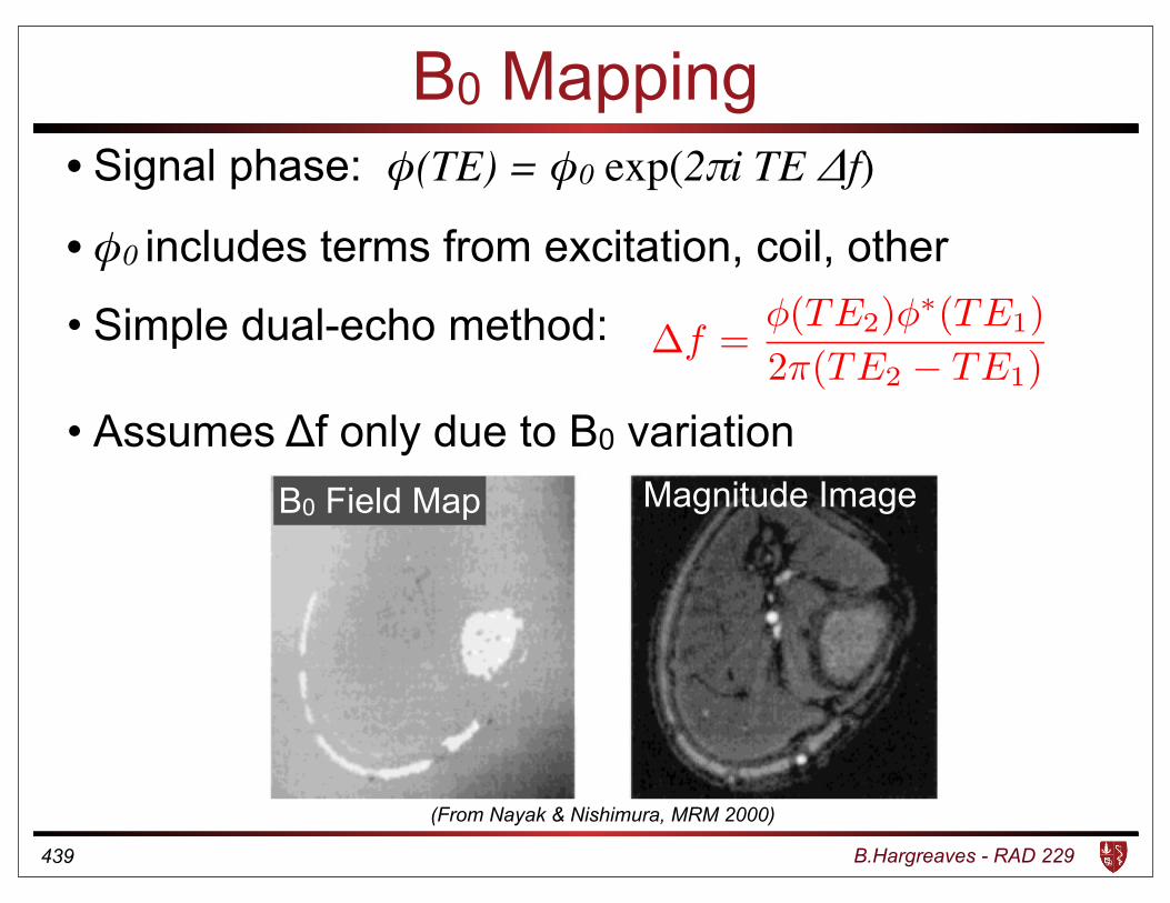
B0 Mapping• Signal phase: φ(TE) = φ0 exp(2πi TE Δf)
• φ0 includes terms from excitation, coil, other
• Simple dual-echo method:
• Assumes Δf only due to B0 variation
439
�f =�(TE2)�⇤(TE1)
2⇡(TE2 � TE1)
Magnitude ImageB0 Field Map
(From Nayak & Nishimura, MRM 2000)
B.Hargreaves - RAD 229
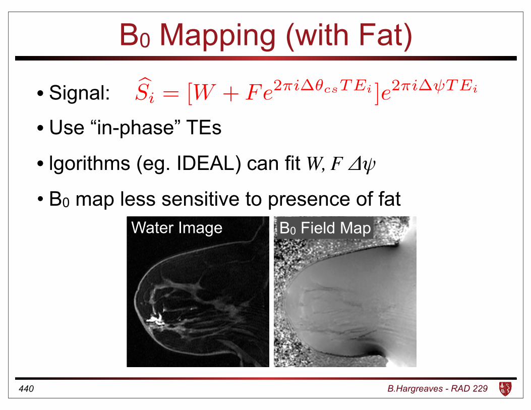
B0 Mapping (with Fat)
• Signal:
• Use “in-phase” TEs
• lgorithms (eg. IDEAL) can fit W, F Δψ
• B0 map less sensitive to presence of fat
440
Water Image B0 Field Map
bSi = [W + Fe2⇡i�✓csTEi ]e2⇡i� TEi
B.Hargreaves - RAD 229
B1 Mapping
• Double-angle method, SDAM (Insko 1993)
• Stimulated Echo
• AFI (Yarnik 2007)
• Phase-sensitive (Morrell 2008)
• Bloch-Siegert (Sacolick 2010)
441
B.Hargreaves - RAD 229
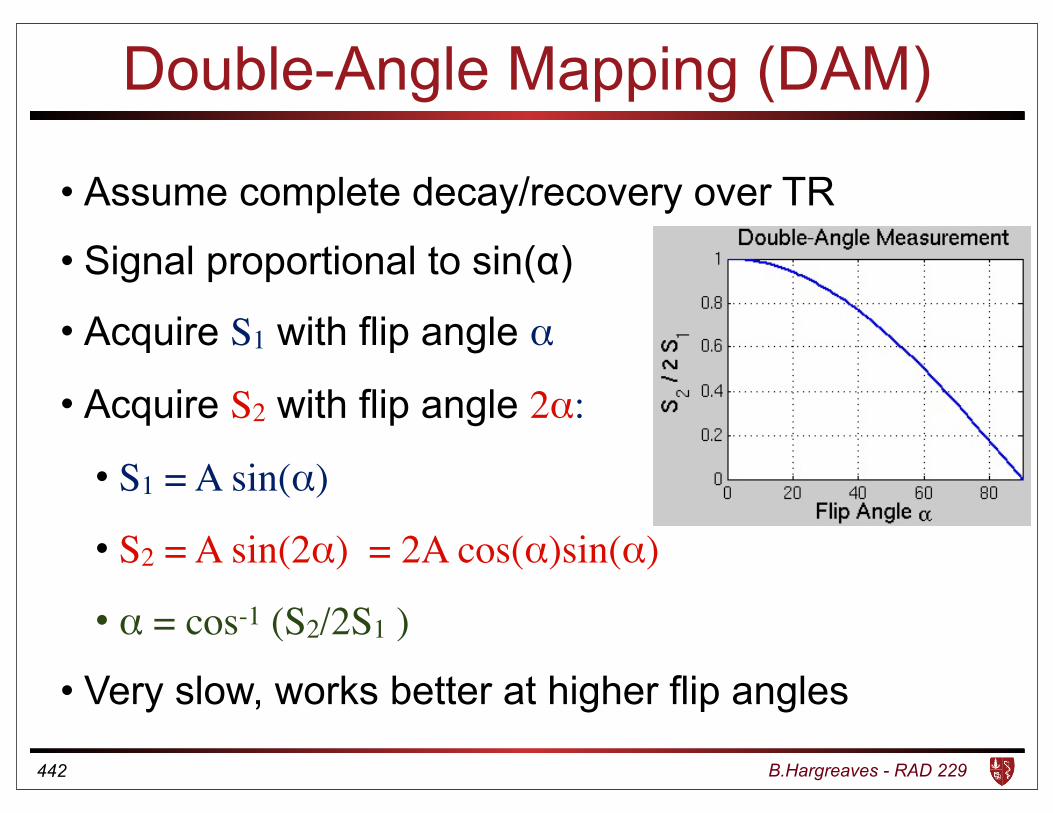
Double-Angle Mapping (DAM)
• Assume complete decay/recovery over TR
• Signal proportional to sin(α)
• Acquire S1 with flip angle α
• Acquire S2 with flip angle 2α:
• S1 = A sin(α)
• S2 = A sin(2α) = 2A cos(α)sin(α)
• α = cos-1 (S2/2S1 )
• Very slow, works better at higher flip angles
442
B.Hargreaves - RAD 229
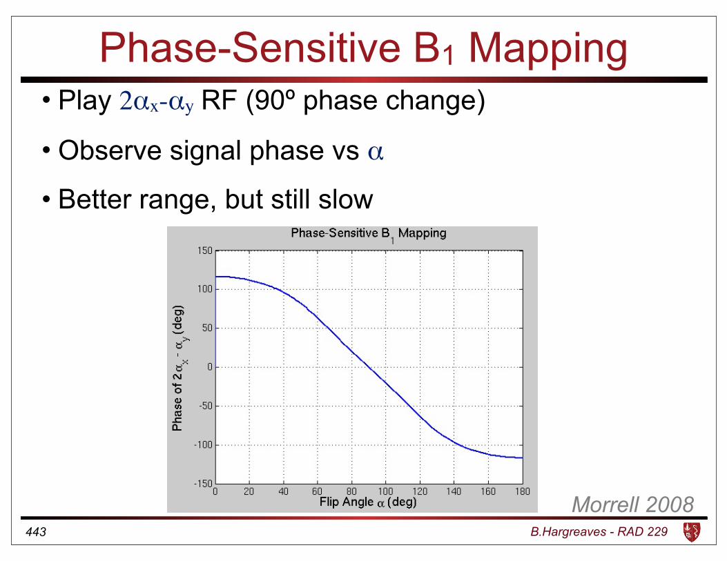
Phase-Sensitive B1 Mapping• Play 2αx-αy RF (90º phase change)
• Observe signal phase vs α
• Better range, but still slow
443
Morrell 2008
B.Hargreaves - RAD 229
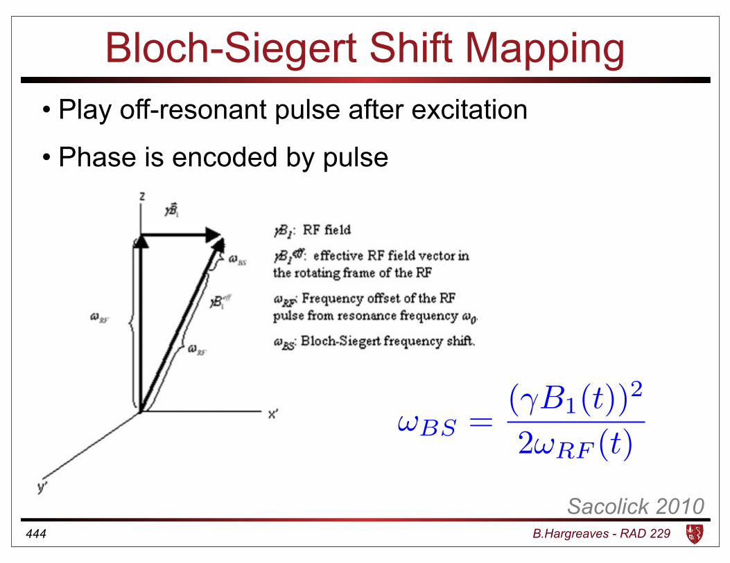
Bloch-Siegert Shift Mapping• Play off-resonant pulse after excitation
• Phase is encoded by pulse
444
Sacolick 2010
!BS =(�B1(t))2
2!RF (t)
B.Hargreaves - RAD 229
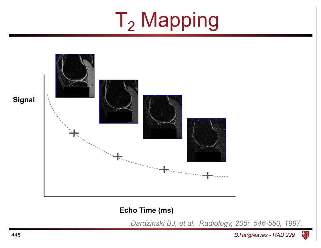
T2 Mapping
Dardzinski BJ, et al. Radiology, 205: 546-550, 1997.
Signal
Echo Time (ms)
TE = 20
TE = 40
TE = 60
TE = 80
445
B.Hargreaves - RAD 229
T2-Mapping Options
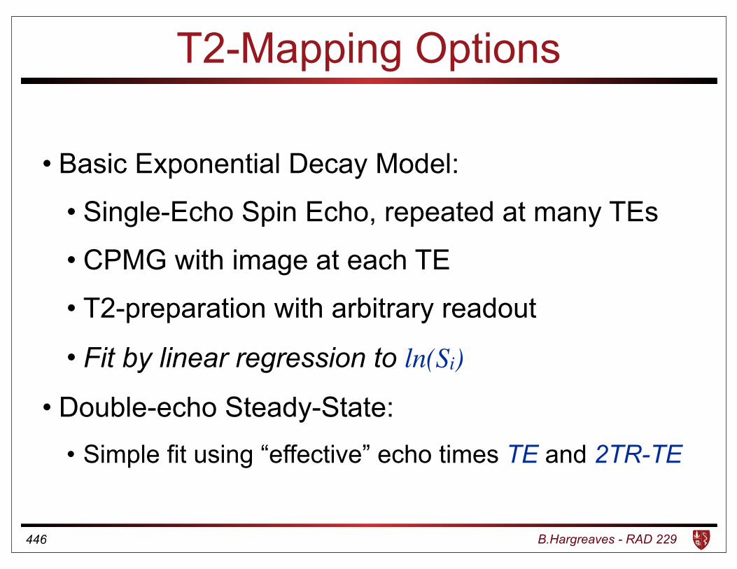
• Basic Exponential Decay Model:
• Single-Echo Spin Echo, repeated at many TEs
• CPMG with image at each TE
• T2-preparation with arbitrary readout
• Fit by linear regression to ln(Si)
• Double-echo Steady-State:• Simple fit using “effective” echo times TE and 2TR-TE
446
B.Hargreaves - RAD 229
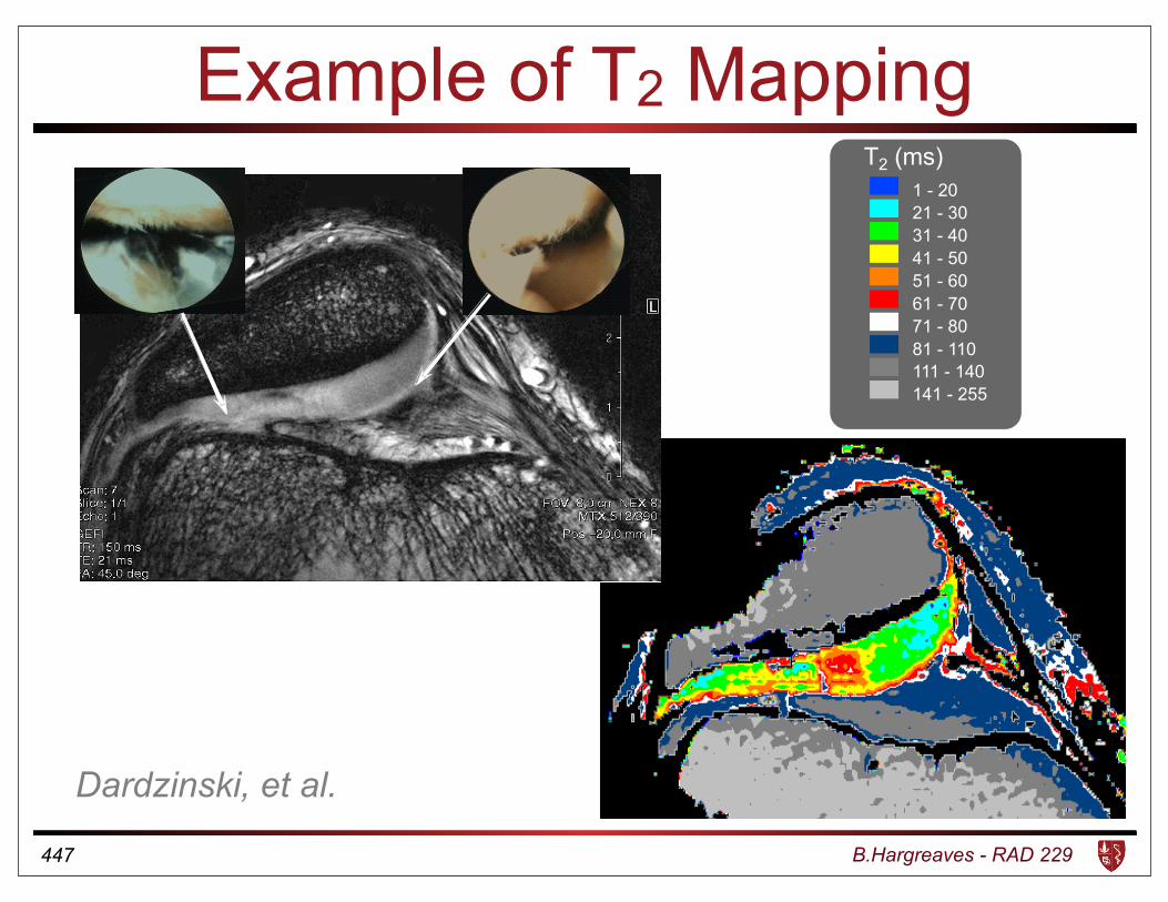
Example of T2 Mapping
Dardzinski, et al.
447
1 - 2021 - 3031 - 4041 - 5051 - 6061 - 7071 - 8081 - 110111 - 140141 - 255
T2 (ms)
B.Hargreaves - RAD 229
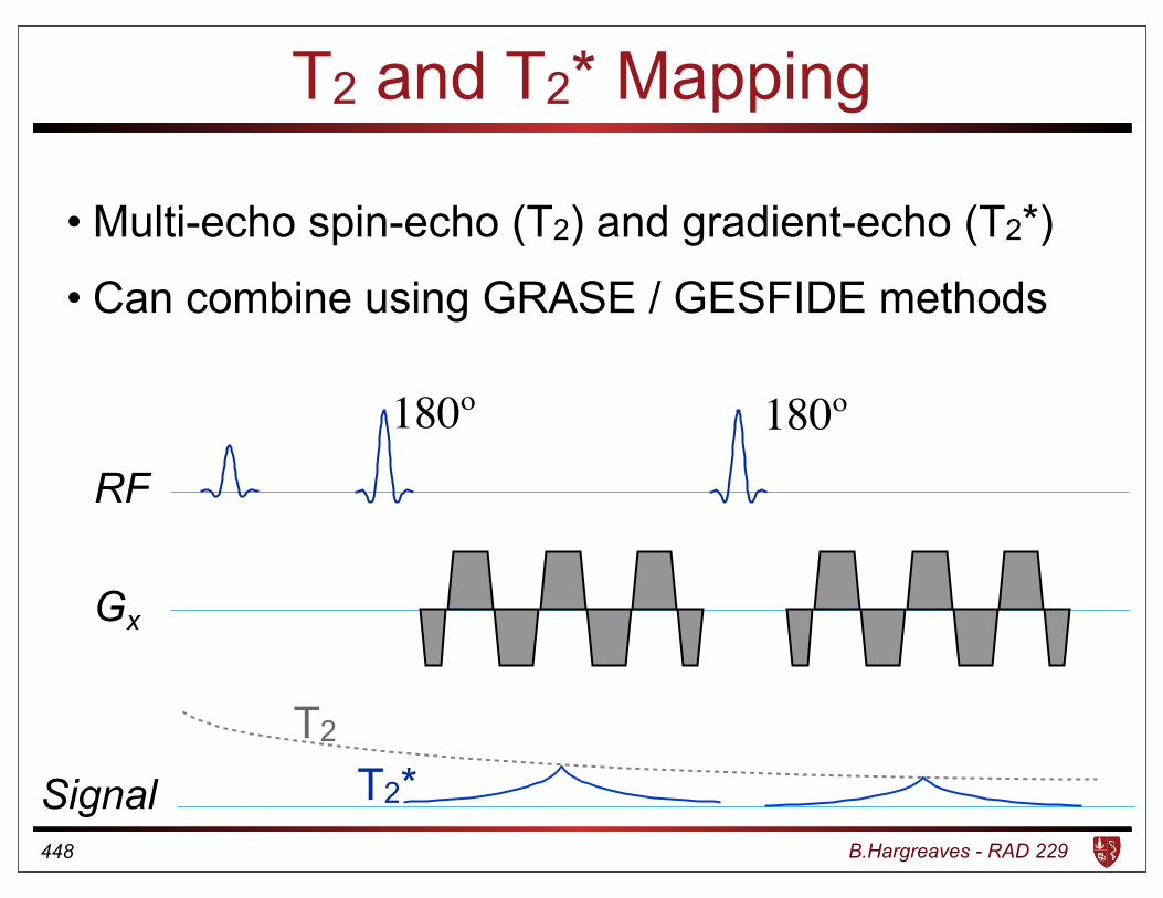
T2 and T2* Mapping
• Multi-echo spin-echo (T2) and gradient-echo (T2*)
• Can combine using GRASE / GESFIDE methods
448
Gx
RF
180º 180º
Signal
T2
T2*
B.Hargreaves - RAD 229
T1 mapping
• IR spin echo
• Saturation-recovery
• Look-locker
• VFA/DESPOT1
• MPnRAGE
449
B.Hargreaves - RAD 229
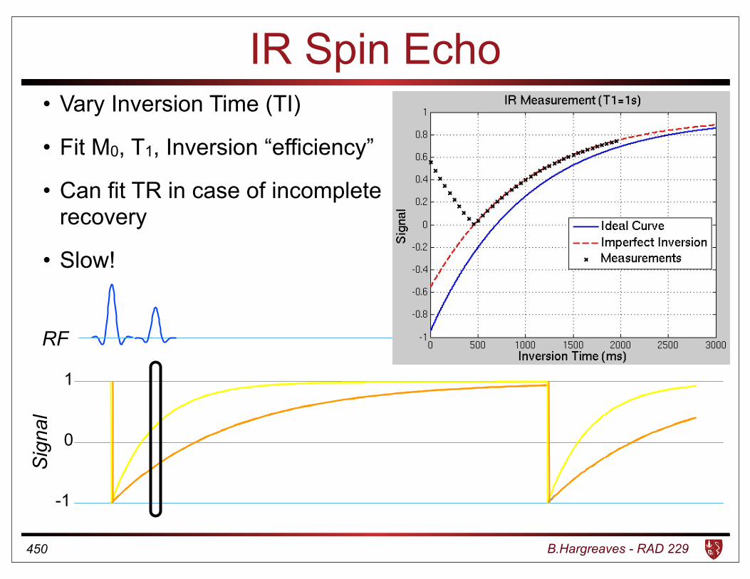
IR Spin Echo• Vary Inversion Time (TI)
• Fit M0, T1, Inversion “efficiency”
• Can fit TR in case of incomplete recovery
• Slow!
450
RF
Sig
nal
1
-1
0
B.Hargreaves - RAD 229
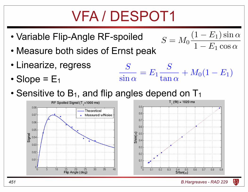
VFA / DESPOT1• Variable Flip-Angle RF-spoiled• Measure both sides of Ernst peak• Linearize, regress• Slope = E1
• Sensitive to B1, and flip angles depend on T1
451
S = M0(1� E1) sin↵
1� E1 cos↵
S
sin↵= E1
S
tan↵+M0(1� E1)
B.Hargreaves - RAD 229
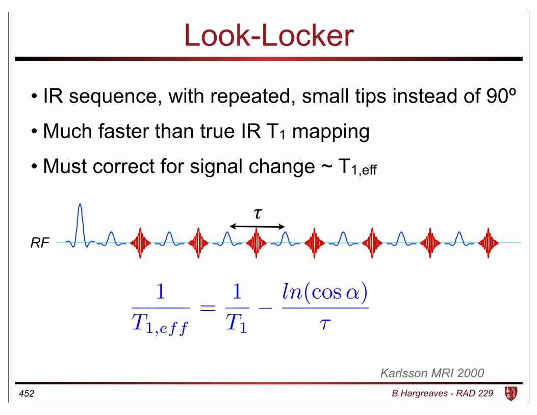
Look-Locker
• IR sequence, with repeated, small tips instead of 90º
• Much faster than true IR T1 mapping
• Must correct for signal change ~ T1,eff
452
1
T1,eff=
1
T1� ln(cos↵)
⌧
RF
Karlsson MRI 2000
τ
B.Hargreaves - RAD 229
MRF ~ “Fingerprinting”
• Apply a “randomized” known sequence
• Simulate signal vs combinations (T1, T2, B0, D, ....)
• Form a dictionary of signal evolutions
• Fit observed signal to dictionary
• Undersample sequence (variable-density spiral)
• Undersampling artifact is not fitted - powerful!
453
Ma et al. 2012
B.Hargreaves - RAD 229
Summary: Quantitative/Mapping Methods
• Gradient Measurement
• Fat/Water Separation
• B0 and B1 mapping
• T1, T2 and T2* mapping
454