Reducción de escala mapas utilizando GIS MODISel caso de las heladas

8/12/2019 Reducción de escala mapas utilizando GIS MODISel caso de las heladas

http://slidepdf.com/reader/full/reduccion-de-escala-mapas-utilizando-gis-modisel-caso-de-las-heladas 1/13

Downscaling MODIS-derived maps using GIS and boosted regression trees: The caseof frost occurrence over the arid Andean highlands of BoliviaRobin Pouteau a ,b , Serge Rambal b , Jean-Pierre Ratte b , Fabien Gogé b , Richard Joffre a ,b , Thierry Winkel a ,⁎

a IRD, CEFE-CNRS, F-34293 Montpellier cedex 5, Franceb UMR 5175, CEFE-CNRS, F-34293 Montpellier cedex 5, France

a b s t r a c ta r t i c l e i n f o

Article history:Received 4 June 2010Received in revised form 17 August 2010Accepted 19 August 2010

Keywords:AltiplanoAndesBoliviaBoosted regression treesDEMDownscalingFrost risk mappingMODISPhysiographyTemperature lapse rateTopoclimate modelSatellite land surface temperature

Seasonal variationSpatial variation

Frost risk assessment is of critical importance in tropical highlands like the Andes where human activitiesthrives at altitudes up to 4200 m, and night frost may occur all the year round. In these semi-arid and coldregions with sparse meteorological networks, remote sensing and topographic modeling are of potentialinterest for understanding how physiography in uences the local climate regime. After integrating night landsurface temperature from the MODIS satellite, and physiographic descriptors derived from a digital elevationmodel, we explored how regional and landscape-scale features in uence frost occurrence in the southernaltiplano of Bolivia. Based on the high correlation between night land surface temperature and minimum airtemperature, frost occurrence in early-, middle- and late-summer periods were calculated from satelliteobservations and mapped at a 1-km resolution over a 45,000 km² area. Physiographic modeling of frostoccurrence was then conducted comparing multiple regression (MR) and boosted regression trees (BRT).Physiographic predictors were latitude, elevation, distance from salt lakes, slope steepness, potentialinsolation, and topographic convergence. Insolation in uence on night frost was tested assuming that groundsurface warming in thedaytime reduces frost occurrence in the next night. Depending on the time period andthe calibration domain, BRTmodels explained 74% to 90% of frost occurrence variation, outperforming the MR method. Inverted BRT models allowed the downscaling of frost occurrence maps at 100-m resolution,illustrating local processes like cold air drainage. Minimum temperature lapse rates showed seasonal

variationand mean valueshigher than those reported fortemperatemountains. When applied at regional andsubregional scales successively, BRT models revealed prominent effects of elevation, latitude and distance tosalt lakes at large scales, whereas slope, topographic convergence and insolation gained in uence at localscales. Our results highlight the role of daytime insolation on night frost occurrence at local scale, particularlyin the early- and mid-summer periods when solar astronomic forcing is maximum. Seasonal variations andinteractions in physiographic effects are also shown. Nested effects of physiographic factors across scales arediscussed, as well as potential applications of physiographic modeling to downscale ecological processes incomplex terrains.

© 2010 Elsevier Inc. All rights reserved.

1. Introduction

Low air temperature is one of the most important factorscontrolling vegetation zonation and key processes such as evapo-transpiration, carbon xation and decomposition, plant productivityandmortality in natural andcultivated mountain ecosystems ( Chen etal., 1999; Nagy et al., 2003 ). Depending on vegetation structure,landscape position or soil properties, frost can damage plant tissuesthus affecting forest, pasture and crop productivity ( Blennow &Lindkvist, 2000 ). These damages have consequences for humanpopulations, particularly in the tropics where highlands often remaindensely populated ( Grötzbach & Stadel, 1997 ). In the Andes of

Argentina, Bolivia, Chile, Ecuador and Peru agriculture thrives ataltitudes up to 4200 m ( Del Castillo et al., 2008 ) and treeline reachesits world's highest elevation up to 5100 m ( Hoch & Körner, 2005 ) inspite of night frost occurringon more than 300 days practically spreadall over the year ( Garcia et al., 2007; Gonzalez et al., 2007; Rada et al.,2009; Troll, 1968 ). In the southern Andes, sparsely vegetated areas juxtaposing extended at plains around salt lakes and steep slopes onthe cordilleras and volcanos, display semi-arid and desert landscapeslargely dominatedby terrain structure. Subjected to thenight/dayandsunlit/shaded slope contrasts characteristic of the mountain climate,this environment is well suited for examiningthe in uence of regionaland landscape-scale physiography on the local climate regime, andparticularly frost occurrence.

Several studies on topoclimate in highlands showed that elevationand slope are the main explanatory variables in modeling localclimate spatial variability ( Chuanyan et al., 2005 ). By means of digital

Remote Sensing of Environment 115 (2011) 117 – 129

⁎ Corresponding author.E-mail address: [email protected] (T. Winkel).

0034-4257/$ – see front matter © 2010 Elsevier Inc. All rights reserved.

doi: 10.1016/j.rse.2010.08.011

Contents lists available at ScienceDirect

Remote Sensing of Environment j o u r n a l h o m ep a g e : w ww. e l sev i e r. c o m/ l o ca t e / r s e

http://dx.doi.org/10.1016/j.rse.2010.08.011



mailto:[email protected]


http://www.sciencedirect.com/science/journal/00344257

http://www.sciencedirect.com/science/journal/00344257


mailto:[email protected]




elevation models and astronomical equations, the potential insolation(incoming solar radiation) has been included as an additionalindependant variable in some of these models, substantially improv-ing their capacity to predict free-air as well as soil-surface temper-ature distributions ( Benavides et al., 2007; Blennow & Lindkvist,2000; Fridley, 2009; Fu & Rich, 2002 ). Among the physiographicvariables, elevation and slope steepness are known to in uence coldair drainage at night and, hence, the distribution of frost risks at

landscape scale ( Lundquist et al., 2008; Pypker et al., 2007a ). In thedaytime, slope aspect and physiographic shading effects control theeffective radiation load per unit of soil areas, resulting in verycontrasted values of daily maximum soil temperature ( Fu & Rich,2002 ). Minimum night temperature might be sensitive to insolationduring the previous day, since soil surface warming during that daycould dampen soil radiative cooling in the next night. Thoughchallenged by studies on minimum air temperature variations inmoderately high mountains under temperate climate ( Blennow,1998; Dobrowski et al., 2009 ), this hypothesis should be tested inthe central part of the Andes, where low latitude, high elevation(typically ranging between 3600 and 4200 m) and sparse vegetationresult in much greater radiation load and thermal contrasts acrossshaded and sunlit areas. Besides, using a downscaling approach,Fridley (2009) noticed that the lack of relationship between daytimeradiation and nighttime temperature is true at local scale lower than1000 m but not at regional scale (Great Smoky Mountains, USA),where variations in radiation balance across locations do in uencenighttime temperature distribution particularly in cooler situations.Considering the Andes, recent work by Bader and Ruijten (2008) andBader et al. (2008) used topographic modeling and remote sensingdata to examine the response of vegetation distribution to climatewarming, but we should go back to Santibañez et al. (1997) andFrançois et al. (1999) to nd studies on the links between frostclimatology and physiography over this region. These early workswere not continued, and the case of the Andean highlands remainedpoorly documented in spite of the potential interest of that region,densely populated and representative of the tropical mountainsvulnerable to global warming ( Vuille et al., 2008 ).

Analyzing topographic effects on free-air or land surface temper-ature also led to reevaluate the simplifying assumption of a genericenvironmental lapse rate (the decrease in free-air temperature aselevation rises, typically assumed to be − 0.6 °C per 100 m),commonly applied in hydrological and ecological studies to extrap-olate air temperature in mountain areas. In fact, several studies showtemperature lapse rate variations due to seasonality, height above theground, or ground surface characteristics ( Blandford et al., 2008;Dobrowski et al., 2009; Fridley, 2009; Lookingbill & Urban, 2003;Marshall et al., 2007 ), though no detailed reports were published forthe Central Andes.

Most of the above mentionned studies used multiple linearregression for modeling the in uence of physiography on free-air orsoil-surface temperatures. The present study resorts to an advanced

form of regression, the boosted regression trees (BRT). BRT use theboosting technique to combine large numbers of relatively simple treemodels to optimize predictive performance. BRT have been usedsuccessfully in human biology ( Friedman & Meulman, 2003 ), landcover mapping ( Lawrence et al., 2004 ), biogeography ( Parisien &Moritz, 2009 ), species distribution ( Elith et al., 2008 ), and soil science(Martin et al., 2009 ). They offer substantial advantages over classicalregression models since they handle both qualitative and quantitativevariables, can accomodate missing data and correlated predictivevariables, are relatively insensitive to outliers and to the inclusion of irrelevant predictor variables, and are able to model complexinteractions between predictors ( Elith et al., 2008; Martin et al.,2009 ). Though direct graphic representation of the complete treemodel is impossible with BRT, the model interpretation is made easy

by identifying the variables most relevant for prediction, and then

visualizing the partial effect of each predictor variable after account-ing for the average effectof the other variables ( Friedman & Meulman,2003 ).

The aims of the present work were: i) to explore how regional andlandscape-scale physiography in uence frost occurrence in Andeanhighlands through integration of eldand remote sensing data, digitalterrain analysis, and GIS; and ii) to downscale regional frostoccurrence maps at a level relevant for farming and land management

decisions using BRT models. This study was focused on the australsummer period, from November to April, when frost holds thegreatest potential impact for local farming activities.

2. Material and methods

2.1. Study area and regional climate

The study area was located at the southwest of the Bolivianhighlands, near the borders of Argentina and Chile, between 19°15 ′

and 22°00 ′ South and between 66°26 ′ and 68°15 ′ West. This region,boarded by the western Andes cordillera, is characterized by thepresence in its centre of a ca.100× 100 km dry salt expanse, the Salarof Uyuni, while another salt lake, the Salar of Coipasa, lies at the northof the study area. The landscapes show a mosaic of three types of landunits: more or less extended at shores surrounding the salt lakes(elevation ca. 3650 m) and an alternation of valleys and volcanicrelieves (culminating at 6051 m) in the hinterland. The nativevegetation of this tropical Andean ecosystem, also known as puna ,consists of a mountain steppe of herbaceous and shrub species (e.g.Baccharis incarum , Parastrephia lepidophylla , and Stipa spp.) ( Navarro& Ferreira, 2007 ) traditionally used as pastures but progressivelyencroached by the recent and rapid expansion of quinoa crop(Chenopodium quinoa Willd.) ( Vassas et al., 2008 ).

Due to its low latitude and high elevation, the study area ischaracterized by a cold and arid tropical climate. Average precipita-tions vary between 100 and 350 mm year − 1 from the South to theNorth of the region ( Geerts et al., 2006 ), presenting an unimodaldistribution with a dry season from April to October. The annualaverage temperature (close to 9 °C) hides daily thermal amplitudeshigher than seasonal amplitudes, of up to 25 °C ( Frère et al., 1978 ).These particular thermal conditions lead to high frost risks throughoutthe year. Advections of air masses from the South Pole represent only20% of the observed frosty nights ( Frère et al., 1978 ) and are fourtimes less frequent in the summer than during the winter, when theintertropical convergence zone goes northward ( Ronchail, 1989 ).Therefore, the main climatic threat lies in radiative frost, occurringduring clear and calm nights. As reported by local peasants, frostoccurence shows a strong topographical and orographical depen-dence, as well as a marked seasonality. This seasonality lead us to splitthe activevegetation period into three time periods characterizing themean regional climate dynamics in the summer rainy season:November – December when precipitation and minimum temperature

rise progressively, January – February when precipitation and temper-ature are at their maximum, and March – April when both begin todecrease.

2.2. Data

2.2.1. Meteorological ground dataIn the study area, daily air temperature records were available in

three meteorological stations: one at Salinas de Garci Mendoza(19°38 ′ S, 67°40′ W) managed by the SENAMHI (Meteorology andHydrology National Service, Bolivia) where daily minimum airtemperature (Tn) was recorded in 1989 and from 1998 to 2006, andtwo others at Irpani (19°45 ′ S, 67°41′ W) and Jirira (19°51 ′ S, 67°34′ W)where meteorological stations set up by the IRD (Research Institute

for Development, France) recorded semi-hourly air temperature from

118 R. Pouteau et al. / Remote Sensing of Environment 115 (2011) 117 –129



23 November 2005 to 18 February 2006 in Irpani, and from 6November 2006 to 31 December 2007 in Jirira. This dataset wastemporally and spatially insuf cient to interpolate frost risks at aregional scale, but it allowed to establish the relationship between airtemperature and remotely sensed land surface temperature.

2.2.2. Remotely sensed dataThe two sensors, Terra and Aqua, of the satellite system MODIS

give daily images of the Earth radiative land surface temperature.Images from the fth version of the MYD11A1 MODIS product wereconcatenated and projected in the UTM-19S (Universal TransverseMercator 19 South) coordinate system using the MODIS projectiontool. In this way, daily 1-km resolution images of the radiative landsurface temperature (Ts) over the study area were obtained. Tsimages recorded by the Aqua sensor around 2 a.m. were used as theywere closer to the Tn data recorded at ground level and closer to thetrue physiological conditions experienced by the vegetation ( Françoiset al., 1999 ). Time series of nominal 1-km spatial resolution MODISdata were downloaded from NASA's EOS data gateway ( https://wist.echo.nasa.gov/ ) from 20 July 2001 to 25 April 2006 and from 01 January 2007 to 31 December 2007. Due to the particular surfaceproperties of the salt lakes of Coipasa and Uyuni in terms of surface

moisture and radiative emissivity, parameter estimations wereconsidered dubious there andTs data for the salt lakes were discardedfrom the analysis. This database was managed and analyzed using theENVI 4.2. software (ITT Visual Information Solutions, www.ittvis.com). The statistical correspondence between Tn data recorded in themeteorological stations of Salinas, Irpani and Jirira and Ts data of thepixels including these three localities was examined by linearregression and Pearson correlation.

Apart from Ts measurements during clear nights, MODIS imagesalso bring information about the possible presence of clouds betweenthe Earth surface and the satellite at the time of the record. Theinformation of these “ agged ” images is valuable for our purposesince radiative frost would not occur during cloudy nights. Thefrequency of cloudy pixels in the daily MODIS images was thus

calculated and used in the frost occurrence calculation.

2.2.3. Digital elevation model and physiographic predictorsThe SRTM digital elevation model ( Farr et al., 2007 ) with a 90 m

horizontal resolution and a vertical accuracy better than 9 m wasusedafter resampling to 100 m to make easier the correspondencebetween the digital elevation model and the MODIS images at 1-kmscale. In a GIS environment using Idrisi Kilimanjaro, Envi 4.2. andArcMap 9.2. softwares, eight physiographic variables were calculated

at a 100-m resolution for each location to examine their potential rolein the spatial determinism of frost and to downscale frost maps tolevels closer to thoseof frost impacts on anthropic activities ( Table 1 ).The compound topographic index (CTI) was used as an index of coldair drainage ( Gessler et al., 2000 ), with low CTI values representingconvex positions like moutain crests and with high CTI valuesrepresenting concave positions like coves or hillslope bases. Threeinsolation variables (DPI, MPI andAPI) were calculated by the ArcMap

9.2. solar analysis tool. They express the amount of radiative energyreceived across all wavelengths over the course of a typical seasonalday (DPI), or from sunrise to 12:00 (MPI), or from 12:00 to sunset(API) of such a day. These insolation variables account for site latitudeand elevation, slope steepness and aspect, daily and seasonal sunangle, andshadows castby surrounding heights. API was calculated toexamine the speci c in uence of insolation in the afternoon justbefore the considered night, with the hypothesis that highsoil surfaceinsolation and warming would affect the soil energybalance, and thusreduce the risk of radiative frost in the following night (withoutregards to other potential factors such as soil albedo, soil watercontent, air humidity, etc. see Garcia et al. (2004) ). Similarly, MPI wascalculated as a surrogate to the early morning insolation, with thehypothesis that areas in the shade of surrounding heights in the earlymorning would experience cooler conditions for a longer time, thusbeing more vulnerable to frost than sunlit areas. In the calibrationprocedure, these 100-m resolution variables were upscaled at 1-kmresolution by averaging 10× 10 pixel clusters in the DEM 100-mimages, thus tting the 1-km resolution of the remotely sensed frostoccurrence maps.

2.3. Physiographic modeling of frost occurrence over regional andsubregional domains

2.3.1. MODIS-derived frost occurrenceFrost is detected by remote sensing when surface temperature

appears negative on cloudfree images. Based on the standardmeteorological threshold of 0 °C, frost occurrence (R) for a speci ctime period was therefore de ned as follows:

R = Prob Ts b 0 - C *F ð1Þ

where: R=frost occurrence at the 0 °C threshold (relative probabilityranging from 0 to 1), Prob (Ts b 0 °C)= probability of the surfaceradiative temperature being lower than 0 °C, F =frequency of cloudless days in the considered period. Note that “frost occurrence ”

is used here instead of frost risk to differentiate our estimates basedon 6-year daily Ts values from climatological estimates based onlonger data series.

Inorder to calculatethe probability Prob (Ts b 0 °C), the distributionof the random variable Ts during successive time periods (namely:November – December, January – February, March – April) was studied,checking its normality through the Kolmogorov – Smirnov test. For

each 1-km pixel andeachtime period, Ts meanandstandarddeviation,cloudless day frequency (F) and, nally, frost occurrence (R) werecalculated from the available nighttime remotely sensed data series(n =366 , 355, and 361 in the ND, JF and MA periods respectively).Maps of observed (remotely sensed) frost occurrence at 1-kmresolution were then generated by applying Eq. (1) for each timeperiod.

2.3.2. Frost occurrence models over regional and subregional domainsA subsample of 1-km pixels ( n =7500) was randomly selected for

the calibration of the physiography – frost occurrence relationshipsover the entire study area (hereafter called “regional models ”).Regional BRT were built for each seasonal period (November –

December, January – February, March – April) using the gbm package

version 1.6-3 developped under R software ( R Development Core

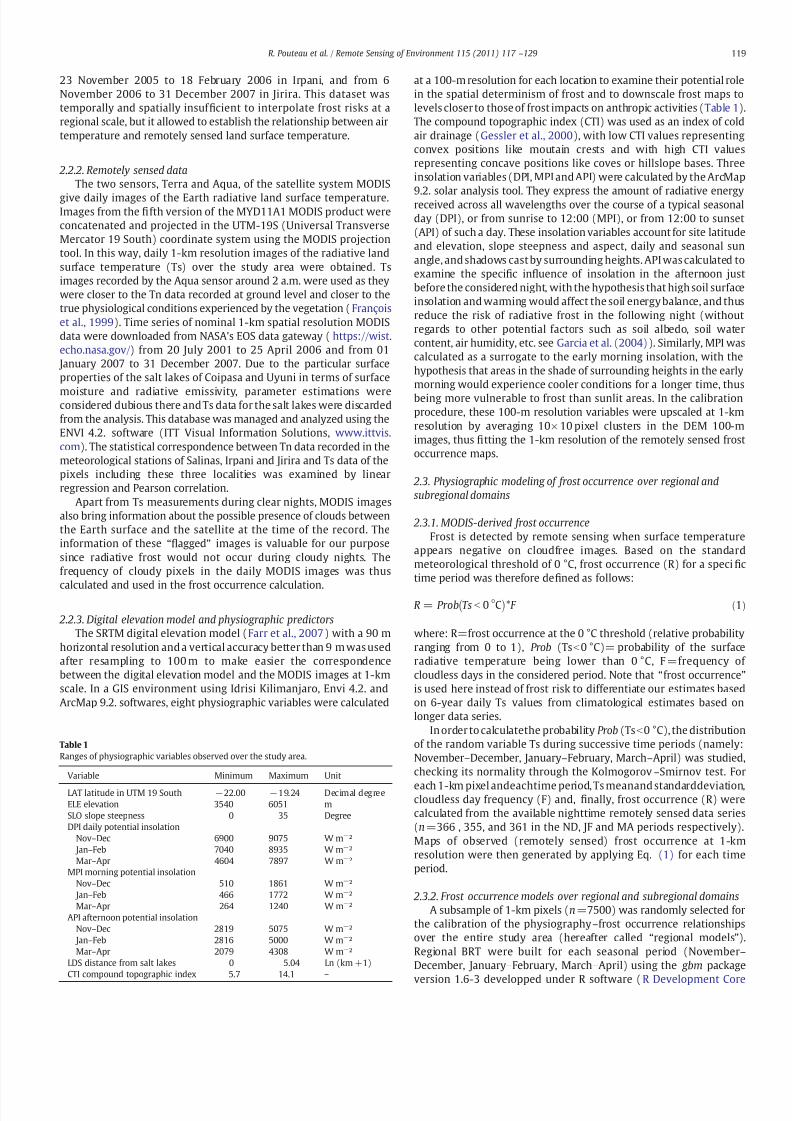
Table 1Ranges of physiographic variables observed over the study area.

Variable Minimum Maximum Unit

LAT latitude in UTM 19 South − 22.00 − 19.24 Decimal degreeELE elevation 3540 6051 mSLO slope steepness 0 35 DegreeDPI daily potential insolation

Nov– Dec 6900 9075 W m − ² Jan– Feb 7040 8935 W m − ²Mar– Apr 4604 7897 W m − ²

MPI morning potential insolationNov– Dec 510 1861 W m − ² Jan– Feb 466 1772 W m − ²Mar– Apr 264 1240 W m − ²

API afternoon potential insolationNov– Dec 2819 5075 W m − ² Jan– Feb 2816 5000 W m − ²Mar– Apr 2079 4308 W m − ²

LDS distance from salt lakes 0 5.04 Ln (km +1)CTI compound topographic index 5.7 14.1 –

119R. Pouteau et al. / Remote Sensing of Environment 115 (2011) 117 –129

https://wist.echo.nasa.gov/


http://www.ittvis.com/


http://-/?-

http://-/?-







Team, 2006 ). A bag fraction of 0.5 was used whichmeans that, at eachstep of the boostingprocedure, 50% of the data inthe trainingset weredrawn at random without replacement. The loss function (LF),de ning the lack-of- t, used a squared-error criterion. The learningrate or shrinkage parameter (LR), the tree size or tree complexity (TS),thenumber of trees (NT)and the minimal numberof observationsperterminal node (MO) were the main parameters for these ttings, andwere set through a tuning procedure ( Martin et al., 2009 ). LR,

determining the contribution of each tree to the model, was thustaken equal to 0.05. NT, the maximal number of trees for optimalprediction was set to 2000. For optimal prediction, TS, the maximalnumber of nodes in the individual trees, was set to a value of 9, andMO was set to 10 observations per terminal node. For sake of comparison, multiple linear regression models were calculated at theregional scale using the same predictors and the same calibrationdatasets as for the regional BRT. These “ regionalMR ” were built usingthe Statistica package ( StatSoft France, 2005 ).

The regional BRT and MR models were validated comparingobserved (remotely sensed) and predicted frost occurrence over theentire study area in the three time periods. This was made excludingthe pixels used for calibration, which resulted in a 49,353 pixelsvalidation set. The predictive capacity of the models was analysedexamining the observed versus predicted values plots, the bias (B),the root mean square error of prediction (RMSE), and the coef cientof determination of the regression between estimated and observedvalues ( R2 ). Once validated, the BRT were interpreted, looking rst atthe relative contribution of the physiographic variables to thepredictive models, and then considering the partial dependence of thepredictions on eachvariable after accounting for theaverage effectof the other variables.

In order to test the scale-dependence of the predictors, a similarBRT procedure was applied over a smaller spatial domainde ned by aselected range of regionally varying factors, namely: latitude between19°5 and 20° South and elevation lower than 4200 m (totalarea=7775 km²). This spatial domain corresponds to the Intersalar ,the area of major agricultural activities in the region, where localpopulations cultivate quinoa and rear camelids up to an altitude of ca.4200 m. A new set of 7500 training pixelswas randomly selected fromthis smaller domain to calibrate these “subregional BRT ”, using thesame values of tting parameters and a similar validation procedureas in the previous analysis. Excluding the training pixels, thisvalidation was conducted on the remaining 275 pixels of this smallerdomain. The relative contribution of the physiographic predictors tothe subregional models was also examined. The interactions betweenpredictive variables were considered by joint plots of their partialdependence in the subregional models.

2.3.3. Downscaling frost occurrence prediction at 100-m resolutionOnce validated, the regional BRT were applied on each pixel of the

DEM 100-m image in order to downscale frost occurrence from 1-kmto 100-m resolution in the three considered time periods. An indirect

validation of these 100-m frost occurrence maps was then conductedby aggregating 10×10 pixel clusters of 100-m frost predictions andcomparing the resulting 1-km predictions to the observed (remotelysensed) frost occurrence at 1-km resolution. A qualitative validationwasalso conducted by examining the capacity of these 100-m maps todisplay well-known local patterns of frost and cold air distributionover complex terrains.

2.3.4. Estimation of the land surface temperature lapse rateThe regression of Ts recorded over sloping areas versus elevation of

the corresponding pixels allowed to calculate average values of theland surface temperature lapse rate at night for successive dates ineach considered time periods. Sloping areas were de ned as terrainswith slope steepness greater than 3° and elevation lower than

5000 m. This elevation limit was chosen to discard high-altitude sites

possibly covered with snow or ice which super cial thermalproperties modify lapse rate estimations ( Marshall et al., 2007 ). Theresulting sampling area represented 22,529 km², covering an eleva-tion range of 1341 m (from 3659 to 5000 m).

3. Results

3.1. Climate information and remotely sensed frost occurrence

evaluationThe frequency analysis of daily minimum air temperature (Tn)

recorded at Salinas over 10 discontinuous years (1989, and the 1998 –

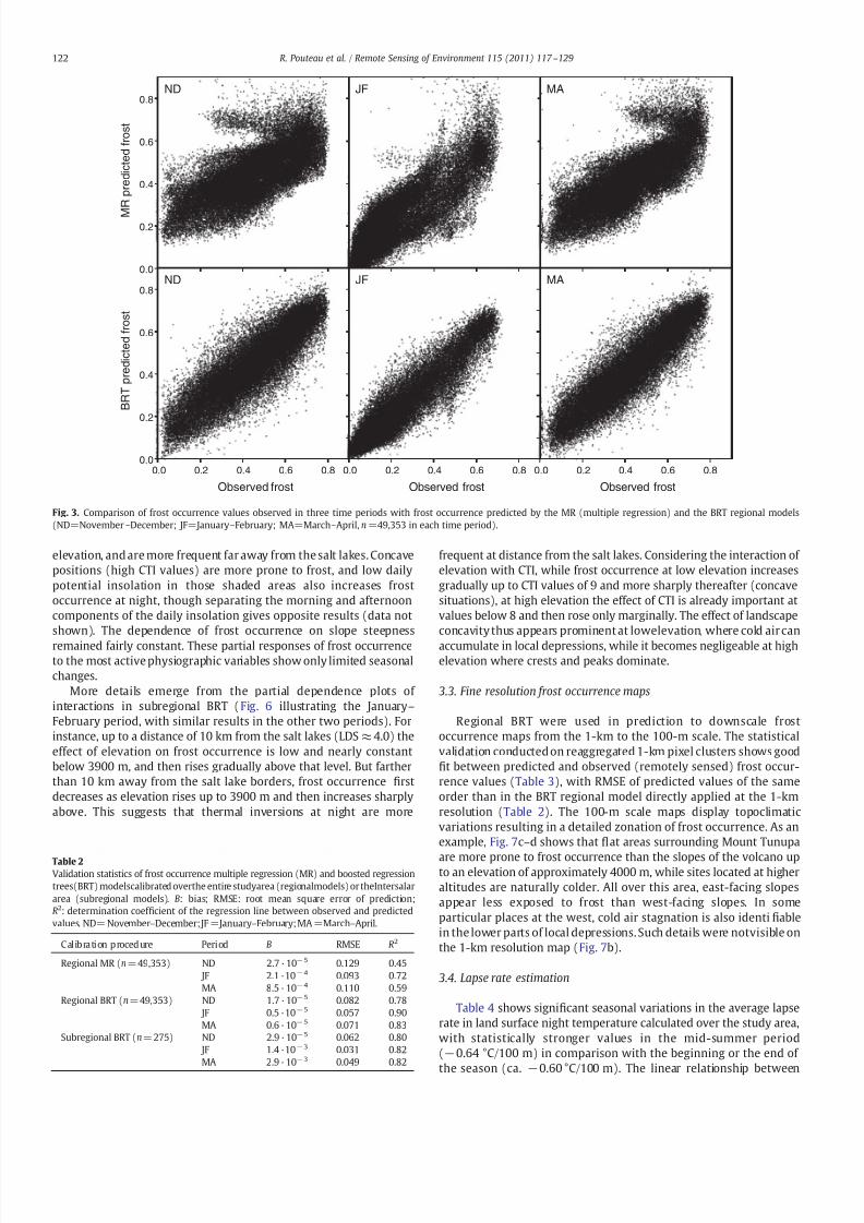
2006 period) was made using the standard climatological thresholdof 0 °C (Fig. 1). During the austral summer (November – April), twoperiods of frequent below zero temperatures surround a ca . 80-daytime interval of lowfrost occurrence, from the beginningof January tothe end of March.

Daily Tn values recorded at screen height by the meteorologicalstations of Salinas, Irpani and Jirira were highly correlated to Ts dataremotely sensed over these three localities at night by the MODISsatellite (Tn=0.97 ⁎ Ts+0.93, R2 =0.81, n =750). The percentage of cloudy pixels on the MODIS images gives a general information aboutthe seasonal pattern of cloud cover in the study area: the January –

February period was the most overcast with on average 46±8.2% of the study area masked by clouds in each daily satellite image, whilethis percentage fell to 30±7.4% and 29±6.6% in the November –

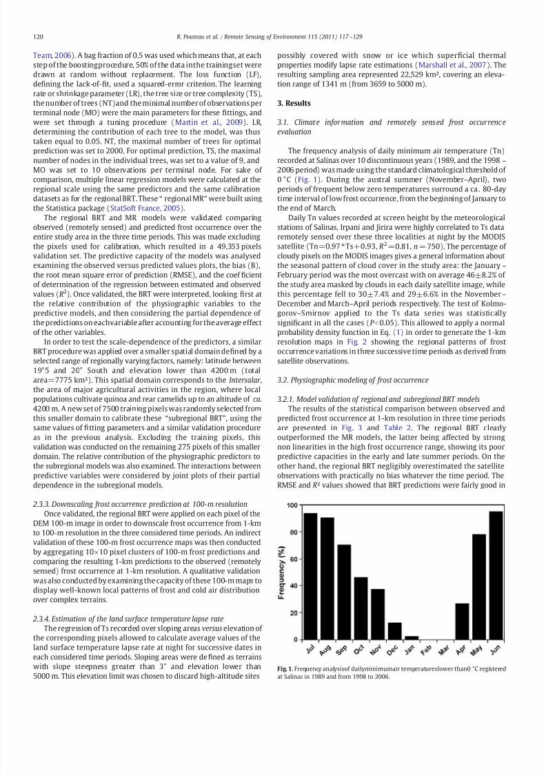
December and March – April periods respectively. The test of Kolmo-gorov – Smirnov applied to the Ts data series was statisticallysigni cant in all the cases ( P b 0.05). This allowed to apply a normalprobability density function in Eq. (1) in order to generate the 1-kmresolution maps in Fig. 2 showing the regional patterns of frostoccurrencevariations in three successive time periods as derived fromsatellite observations.

3.2. Physiographic modeling of frost occurrence

3.2.1. Model validation of regional and subregional BRT modelsThe results of the statistical comparison between observed and

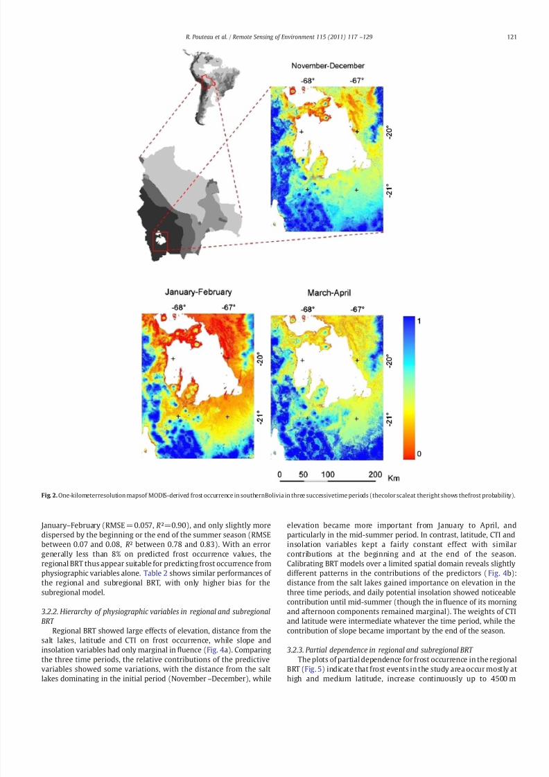
predicted frost occurrence at 1-km resolution in three time periodsare presented in Fig. 3 and Table 2. The regional BRT clearlyoutperformed the MR models, the latter being affected by strongnon linearities in the high frost occurrence range, showing its poorpredictive capacities in the early and late summer periods. On theother hand, the regional BRT negligibly overestimated the satelliteobservations with practically no bias whatever the time period. TheRMSE and R² values showed that BRT predictions were fairly good in

Fig. 1. Frequency analysisof dailyminimumair temperatureslower than0 °C registered

at Salinas in 1989 and from 1998 to 2006.


http://-/?-

http://-/?-



January– February (RMSE =0.057, R²=0.90), and only slightly moredispersed by the beginning or the end of the summer season (RMSE

between 0.07 and 0.08, R² between 0.78 and 0.83). With an errorgenerally less than 8% on predicted frost occurrence values, theregional BRT thus appear suitable for predicting frost occurrence fromphysiographic variables alone. Table 2 shows similar performances of the regional and subregional BRT, with only higher bias for thesubregional model.

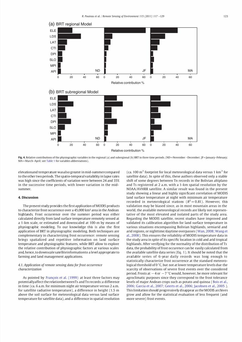
3.2.2. Hierarchy of physiographic variables in regional and subregionalBRT

Regional BRT showed large effects of elevation, distance from thesalt lakes, latitude and CTI on frost occurrence, while slope andinsolation variables had only marginal in uence ( Fig. 4a). Comparingthe three time periods, the relative contributions of the predictivevariables showed some variations, with the distance from the salt

lakes dominating in the initial period (November – December), while

elevation became more important from January to April, andparticularly in the mid-summer period. In contrast, latitude, CTI and

insolation variables kept a fairly constant effect with similarcontributions at the beginning and at the end of the season.Calibrating BRT models over a limited spatial domain reveals slightlydifferent patterns in the contributions of the predictors ( Fig. 4b):distance from the salt lakes gained importance on elevation in thethree time periods, and daily potential insolation showed noticeablecontribution until mid-summer (though the in uence of its morningand afternoon components remained marginal). The weights of CTIand latitude were intermediate whatever the time period, while thecontribution of slope became important by the end of the season.

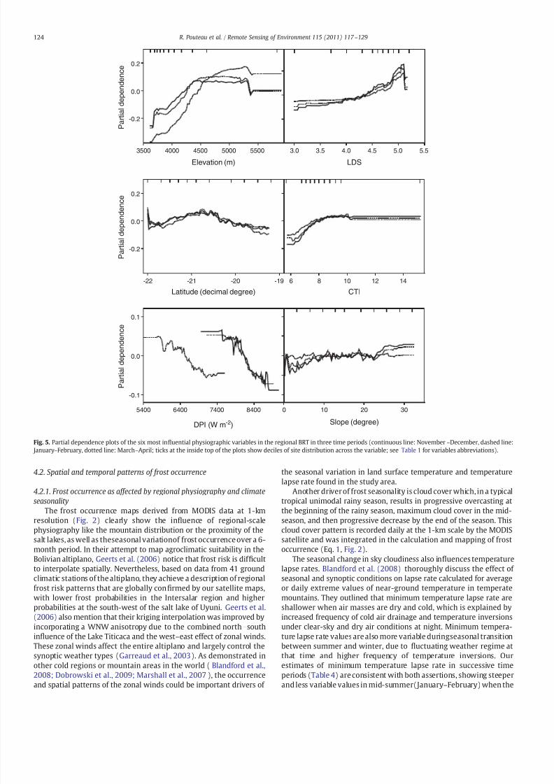
3.2.3. Partial dependence in regional and subregional BRT The plots of partial dependence for frost occurrence in the regional

BRT (Fig. 5) indicate that frost events in the study area occur mostly at

high and medium latitude, increase continuously up to 4500 m

Fig. 2. One-kilometerresolution mapsof MODIS-derived frost occurrence in southernBolivia in three successivetime periods (thecolor scaleat theright shows thefrost probability).


http://localhost/var/www/apps/conversion/tmp/scratch_1/image%20of%20Fig.%E0%B2%80



elevation, andare more frequent far away from thesalt lakes. Concavepositions (high CTI values) are more prone to frost, and low dailypotential insolation in those shaded areas also increases frostoccurrence at night, though separating the morning and afternooncomponents of the daily insolation gives opposite results (data notshown). The dependence of frost occurrence on slope steepnessremained fairly constant. These partial responses of frost occurrenceto the most activephysiographic variables show only limited seasonalchanges.

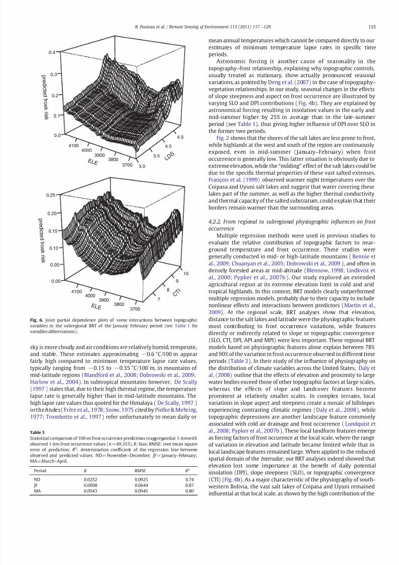
More details emerge from the partial dependence plots of interactions in subregional BRT ( Fig. 6 illustrating the January –

February period, with similar results in the other two periods). Forinstance, up to a distance of 10 km from the salt lakes (LDS ≈ 4.0) theeffect of elevation on frost occurrence is low and nearly constantbelow 3900 m, and then rises gradually above that level. But fartherthan 10 km away from the salt lake borders, frost occurrence rstdecreases as elevation rises up to 3900 m and then increases sharplyabove. This suggests that thermal inversions at night are more

frequent at distance from the salt lakes. Considering the interaction of elevation with CTI, while frost occurrence at low elevation increasesgradually up to CTI values of 9 and more sharply thereafter (concavesituations), at high elevation the effect of CTI is already important atvalues below 8 and then rose only marginally. The effect of landscapeconcavity thus appears prominent at lowelevation, where cold air canaccumulate in local depressions, while it becomes negligeable at highelevation where crests and peaks dominate.

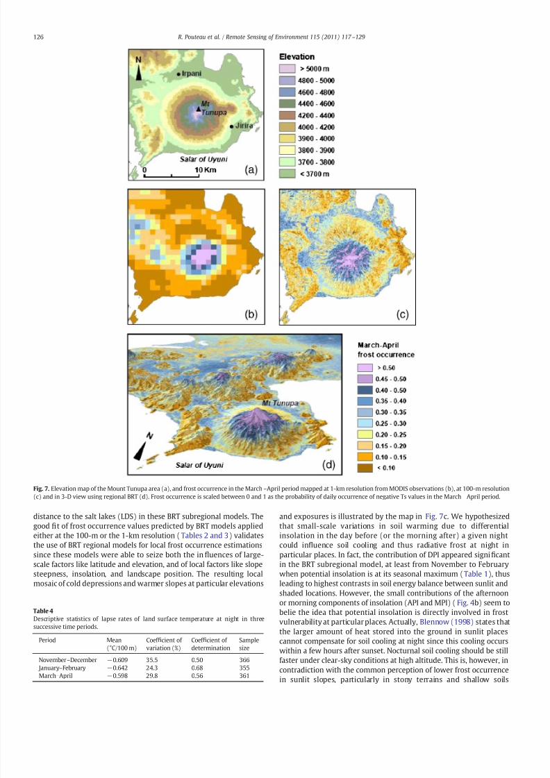
3.3. Fine resolution frost occurrence maps

Regional BRT were used in prediction to downscale frostoccurrence maps from the 1-km to the 100-m scale. The statisticalvalidation conductedon reaggregated 1-km pixel clusters shows good

t between predicted and observed (remotely sensed) frost occur-rence values ( Table 3), with RMSE of predicted values of the sameorder than in the BRT regional model directly applied at the 1-kmresolution ( Table 2). The 100-m scale maps display topoclimaticvariations resulting in a detailed zonation of frost occurrence. As anexample, Fig. 7c– d shows that at areas surrounding Mount Tunupa

are more prone to frost occurrence than the slopes of the volcano upto an elevation of approximately 4000 m, while sites located at higheraltitudes are naturally colder. All over this area, east-facing slopesappear less exposed to frost than west-facing slopes. In someparticular places at the west, cold air stagnation is also identi ablein the lower parts of local depressions.Such details were notvisible onthe 1-km resolution map ( Fig. 7b).

3.4. Lapse rate estimation

Table 4 shows signi cant seasonal variations in the average lapserate in land surface night temperature calculated over the study area,with statistically stronger values in the mid-summer period( − 0.64 °C/100 m) in comparison with the beginning or the end of

the season (ca. − 0.60 °C/100 m). The linear relationship between

0.0

0.2

0.4

0.6

0.8ND

M

R p r e

d i c t e d f r o s

t

JF MA

0.0 0.2 0.4 0.6 0.80.0

0.2

0.4

0.6

0.8ND

Observed frost

B R T p r e

d i c t e d f r o s

t

0.0 0.2 0.4 0.6 0.8

JF

Observed frost0.0 0.2 0.4 0.6 0.8

MA

Observed frost

Fig. 3. Comparison of frost occurrence values observed in three time periods with frost occurrence predicted by the MR (multiple regression) and the BRT regional models(ND=November – December; JF=January – February; MA=March – April, n =49,353 in each time period).

Table 2Validation statistics of frost occurrence multiple regression (MR) and boosted regressiontrees(BRT) modelscalibrated overthe entire studyarea (regionalmodels) or theIntersalararea (subregional models). B: bias; RMSE: root mean square error of prediction;R2 : determination coef cient of the regression line between observed and predictedvalues. ND= November – December; JF =January – February; MA =March – April.

Calibration procedure Period B RMSE R2

Regional MR (n =49,353) ND 2.7 ·10 − 5 0.129 0.45 JF 2.1 ·10 − 4 0.093 0.72MA 8.5 ·10 − 4 0.110 0.59

Regional BRT (n =49,353) ND 1.7 ·10 − 5 0.082 0.78 JF 0.5 ·10 − 5 0.057 0.90MA 0.6 ·10 − 5 0.071 0.83

Subregional BRT (n =275) ND 2.9 ·10 − 5 0.062 0.80 JF 1.4 ·10 − 3 0.031 0.82MA 2.9 ·10 − 3 0.049 0.82



























































elevationand temperature wasalso greater in mid-summercomparedto the other two periods. The spatio-temporalvariability in lapse rateswas high since the coef cients of variation were between 24 and 35%in the successive time periods, with lower variation in the mid-summer.

4. Discussion

The present study provides the rst application of MODIS productsto characterize frost occurrence over a 45,000 km² area in the Andeanhighlands. Frost occurrence over the summer period was eithercalculated directly from land surface temperature remotely sensed ata 1-km scale, or estimated and downscaled at 100-m by means of physiographic modeling. To our knowledge this is also the rstapplication of BRT in physiographic modeling. Both techniques arecomplementary in characterizing frost occurrence: remote sensing

brings spatialized and repetitive information on land surfacetemperature and physiographic features, while BRT allow to explorethe relative contribution of physiographic factors at various scalesand, hence, to downscale satelliteinformationto a level appropriate tofarming and land management applications.

4.1. Application of remote sensing data for frost occurrencecharacterization

As pointed by François et al. (1999) at least three factors maypotentiallyaffect the relationbetweenTs andTn records:a differencein time (ca. 6 a.m. for minimum night air temperature versus 2 a.m.for satellite radiative temperature), a difference in height (1.5 mabove the soil surface for meteorological data versus land surface

temperature for satellite data), and a difference in spatial resolution

(ca. 100 m 2 footprint for local meteorological data versus 1 km 2 forsatellite data). In spite of this, these authors observed only a stableshift of some degrees between Tn records in the Bolivian altiplanoand Ts registered at 2 a.m. with a 1-km spatial resolution by theNOAA/AVHRR satellite. A similar result was found in the presentstudy showing a linear and highly signi cant correlation of MODISland surface temperature at night with minimum air temperaturerecorded in meteorological stations ( R2 = 0.81). However, thisvalidation may be biased since, as in most mountain areas in theworld, the available meteorological records are likely not represen-tative of the most elevated and isolated parts of the study area.Regarding the MODIS satellite, recent studies have improved andvalidated its calibration algorithm for land surface temperature invarious situations encompassing Bolivian highlands, semiarid andarid regions, or nighttime/daytime overpasses ( Wan, 2008; Wang etal., 2008). This ensures the reliability of MODIS temperature data in

the study area in spite of its speci c location in cold and arid tropicalhighlands. After verifying for the normality of the distribution of Tsdata, the probability of frost occurence can be easily calculated fromthe available satellite data series (Eq. 1). It should be noted that theavailable series of 6-year daily records was long enough tostatistically characterize frost occurrence at the standard meteoro-logical threshold of 0 °C, but not at lower temperature levels due thescarcity of observations of severe frost events over the consideredperiod. Frosts at − 4 or − 7 °C would, however, be more relevant foragroclimatic purposes since they correspond to the frost tolerancelevels of major Andean crops such as potato and quinoa ( Bois et al.,2006; Garcia et al., 2007; Geerts et al., 2006; Jacobsen et al., 2005 ).This limitation should progressively disappear as the MODIS archivesgrow and allow for the statistical evaluation of less frequent (and

more severe) frost events.

0 20 40 60

API

MPISLO

DPI

CTI

LAT

LDS

ELE

ND

0 20 40 60

JF

Relative contribution %

0 20 40 60

MA

0 20 40 60

API

MPI

SLO

DPI

CTI

LAT

LDS

ELE

ND

0 20 40 60

JF

0 20 40 60

MA

(b) BRT subregional Model

(a) BRT regional Model

Relative contribution %

Fig. 4. Relative contributions of the physiographic variables in the regional (a) and subregional (b) BRT in three time periods. (ND=November – December; JF=January – February;MA=March – April; see Table 1 for variables abbreviations).


http://-/?-

http://-/?-



4.2. Spatial and temporal patterns of frost occurrence

4.2.1. Frost occurrence as affected by regional physiography and climateseasonality

The frost occurrence maps derived from MODIS data at 1-kmresolution ( Fig. 2) clearly show the in uence of regional-scalephysiography like the mountain distribution or the proximity of thesalt lakes, as well as theseasonal variationof frost occurrenceover a 6-

month period. In their attempt to map agroclimatic suitability in theBolivian altiplano, Geerts et al. (2006) notice that frost risk is dif cultto interpolate spatially. Nevertheless, based on data from 41 groundclimatic stations of thealtiplano, they achieve a description of regionalfrost risk patterns that are globally con rmed by our satellite maps,with lower frost probabilities in the Intersalar region and higherprobabilities at the south-west of the salt lake of Uyuni. Geerts et al.(2006) also mention that their kriging interpolation was improved byincorporating a WNW anisotropy due to the combined north – southin uence of the Lake Titicaca and the west – east effect of zonal winds.These zonal winds affect the entire altiplano and largely control thesynoptic weather types ( Garreaud et al., 2003 ). As demonstrated inother cold regions or mountain areas in the world ( Blandford et al.,2008; Dobrowski et al., 2009; Marshall et al., 2007 ), the occurrence

and spatial patterns of the zonal winds could be important drivers of

the seasonal variation in land surface temperature and temperaturelapse rate found in the study area.

Another driverof frost seasonality is cloud cover which, in a typicaltropical unimodal rainy season, results in progressive overcasting atthe beginning of the rainy season, maximum cloud cover in the mid-season, and then progressive decrease by the end of the season. Thiscloud cover pattern is recorded daily at the 1-km scale by the MODISsatellite and was integrated in the calculation and mapping of frost

occurrence (Eq. 1, Fig. 2).The seasonal change in sky cloudiness also in uences temperature

lapse rates. Blandford et al. (2008) thoroughly discuss the effect of seasonal and synoptic conditions on lapse rate calculated for averageor daily extreme values of near-ground temperature in temperatemountains. They outlined that minimum temperature lapse rate areshallower when air masses are dry and cold, which is explained byincreased frequency of cold air drainage and temperature inversionsunder clear-sky and dry air conditions at night. Minimum tempera-ture lapse rate valuesarealso more variable duringseasonal transitionbetween summer and winter, due to uctuating weather regime atthat time and higher frequency of temperature inversions. Ourestimates of minimum temperature lapse rate in successive timeperiods ( Table 4 ) areconsistent with both assertions, showing steeper

and less variable values in mid-summer(January – February) when the

3500 4000 4500 5000 5500

-0.2

0.0

0.2

Elevation (m)

P a r t i a

l d e p e n

d e n c e

3.0 3.5 4.0 4.5 5.0 5.5

LDS

-22 -21 -20 -19

-0.2

0.0

0.2

Latitude (decimal degree)

P a r t i a

l d e p e n

d e n c e

6 8 10 12 14

CTI

5400 6400 7400 8400

-0.1

0.0

0.1

P a r t i a

l d e p e n

d e n c e

0 10 20 30Slope (degree)DPI (W m -2)

Fig. 5. Partial dependence plots of the six most in uential physiographic variables in the regional BRT in three time periods (continuous line: November – December, dashed line: January– February, dotted line: March – April; ticks at the inside top of the plots show deciles of site distribution across the variable; see Table 1 for variables abbreviations).


http://-/?-

http://-/?-



sky is more cloudy and air conditions are relatively humid, temperate,and stable. These estimates approximating − 0.6 °C/100 m appearfairly high compared to minimum temperature lapse rate values,typically ranging from − 0.15 to − 0.35 °C/100 m, in mountains of mid-latitude regions ( Blandford et al., 2008; Dobrowski et al., 2009;Harlow et al., 2004 ). In subtropical mountains however, De Scally(1997 ) states that, due to their high thermal regime, the temperature

lapse rate is generally higher than in mid-latitude mountains. Thehigh lapse rate values thus quoted for the Himalaya ( De Scally, 1997 )ortheAndes( Frère et al., 1978; Snow, 1975 cited by Pielke & Mehring,1977; Trombotto et al., 1997 ) refer unfortunately to mean daily or

mean annual temperatures which cannot be compared directly to ourestimates of minimum temperature lapse rates in speci c timeperiods.

Astronomic forcing is another cause of seasonality in thetopography – frost relationship, explaining why topographic controls,usually treated as stationary, show actually pronounced seasonalvariations, as pointed by Deng et al. (2007) in the case of topography –

vegetation relationships. In our study, seasonal changes in the effects

of slope steepness and aspect on frost occurrence are illustrated byvarying SLO and DPI contributions ( Fig. 4b). They are explained byastronomical forcing resulting in insolation values in the early andmid-summer higher by 25% in average than in the late-summerperiod (see Table 1), thus giving higher in uence of DPI over SLO inthe former two periods.

Fig. 2 shows that the shores of the salt lakes are less prone to frost,while highlands at the west and south of the region are continuouslyexposed, even in mid-summer (January – February) when frostoccurrence is generally low. This latter situation is obviously due toextreme elevation, while the “milding ” effect of the salt lakes could bedue to the speci c thermal properties of these vast salted extenses.François et al. (1999) observed warmer night temperatures over theCoipasa and Uyuni salt lakes and suggest that water covering theselakes part of the summer, as well as the higher thermal conductivityand thermal capacity of the salted substratum, could explain that theirborders remain warmer than the surrounding areas.

4.2.2. From regional to subregional physiographic in uences on frost occurrence

Multiple regression methods were used in previous studies toevaluate the relative contribution of topographic factors to near-ground temperature and frost occurrence. These studies weregenerally conducted in mid- or high-latitude mountains ( Bennie etal., 2009; Chuanyan et al., 2005; Dobrowski et al., 2009 ), and often indensely forested areas at mid-altitude ( Blennow, 1998; Lindkvist etal., 2000; Pypker et al., 2007b ). Our study explored an extendedagricultural region at its extreme elevation limit in cold and aridtropical highlands. In this context, BRT models clearly outperformedmultiple regression models, probably due to their capacity to includenonlinear effects and interactions between predictors ( Martin et al.,2009 ). At the regional scale, BRT analyses show that elevation,distance to the salt lakes and latitude were the physiographic featuresmost contributing to frost occurrence variations, while featuresdirectly or indirectly related to slope or topographic convergence(SLO, CTI, DPI, API and MPI) were less important. These regional BRTmodels based on physiographic features alone explain between 78%and 90% of the variation in frost occurrence observed in different timeperiods ( Table 2). In their study of the in uence of physiography onthe distribution of climate variables across the United States, Daly etal. (2008) outline that the effects of elevation and proximity to largewater bodies exceed those of other topographic factors at large scales,whereas the effects of slope and landcover features become

prominent at relatively smaller scales. In complex terrains, localvariations in slope aspect and steepness create a mosaic of hillslopesexperiencing contrasting climatic regimes ( Daly et al., 2008 ), whiletopographic depressions are another landscape feature commonlyassociated with cold air drainage and frost occurrence ( Lundquist etal., 2008; Pypker et al., 2007b ). These local landform features emergeas forcing factors of frost occurence at the local scale, where the rangeof variation in elevation and latitude became limited while that inlocal landscape features remained large. When applied to the reducedspatial domain of the Intersalar , our BRT analyses indeed showed thatelevation lost some importance at the bene t of daily potentialinsolation (DPI), slope steepness (SLO), or topographic convergence(CTI) (Fig. 4b). As a major characteristic of the physiography of south-western Bolivia, the vast salt lakes of Coipasa and Uyuni remained

in uential at that local scale, as shown by the high contribution of the

L D S

3.0

3.5

4.0

4.5

E L E 37003800

39004000

4100

p r e d i c t e d

f r o s k r i s k

0.0

0.1

0.2

0.3

0.4

C T I

7

8

9

10

E L E 380039004000

4100

p r e d i c t e d f r o s k r i s k

0.00

0.05

0.10

0.15

0.20

0.25

3700

Fig. 6. Joint partial dependence plots of some interactions between topographicvariables in the subregional BRT of the January – February period (see Table 1 forvariables abbreviations).

Table 3Statistical comparison of 100-m frost occurrence predictions reaggregatedat 1-kmwithobserved 1-km frost occurrence values ( n =49,353). B: bias; RMSE: root mean squareerror of prediction; R2 : determination coef cient of the regression line betweenobserved and predicted values. ND= November – December; JF= January – February;MA=March – April.

Period B RMSE R2

ND 0.0252 0.0925 0.74 JF 0.0008 0.0644 0.87MA 0.0543 0.0945 0.80




distance to the salt lakes (LDS) in these BRT subregional models. Thegood t of frost occurrence values predicted by BRT models appliedeither at the 100-m or the 1-km resolution ( Tables 2 and 3 ) validates

the use of BRT regional models for local frost occurrence estimationssince these models were able to seize both the in uences of large-scale factors like latitude and elevation, and of local factors like slopesteepness, insolation, and landscape position. The resulting localmosaic of cold depressionsand warmer slopes at particular elevations

and exposures is illustrated by the map in Fig. 7c. We hypothesizedthat small-scale variations in soil warming due to differentialinsolation in the day before (or the morning after) a given night

could in uence soil cooling and thus radiative frost at night inparticular places. In fact, the contribution of DPI appeared signi cantin the BRT subregional model, at least from November to Februarywhen potential insolation is at its seasonal maximum ( Table 1), thusleading to highest contrasts in soil energy balance between sunlit andshaded locations. However, the small contributions of the afternoonor morning components of insolation (API and MPI) ( Fig. 4b) seem tobelie the idea that potential insolation is directly involved in frostvulnerability at particularplaces. Actually, Blennow (1998) states thatthe larger amount of heat stored into the ground in sunlit placescannot compensate for soil cooling at night since this cooling occurswithin a few hours after sunset. Nocturnal soil cooling should be stillfaster under clear-sky conditions at high altitude. This is, however, incontradiction with the common perception of lower frost occurrence

in sunlit slopes, particularly in stony terrains and shallow soils

Fig. 7. Elevation map of the Mount Tunupa area (a), and frost occurrence in the March – April period mapped at 1-km resolution from MODIS observations (b), at 100-m resolution(c) and in 3-D view using regional BRT (d). Frost occurrence is scaled between 0 and 1 as the probability of daily occurrence of negative Ts values in the March – April period.

Table 4Descriptive statistics of lapse rates of land surface temperature at night in threesuccessive time periods.

Period Mean(°C/100 m)

Coef cient of variation (%)

Coef cient of determination

Samplesize

November – December − 0.609 35.5 0.50 366 January– February − 0.642 24.3 0.68 355March– April − 0.598 29.8 0.56 361




supposed to bene t from the thermal stability provided by the rocks.Microclimate stability associated to rock outcrops has been docu-mented by Rada et al. (2009) in the paramo ecosystem of VenezuelianAndes at lower elevation (3800 m) and under wetter conditions(969 mm of annual precipitation). It is likely that the much drierconditions of the puna ecosystem in southern Bolivia reduce thethermal inertia of the soils, thus leading to a very fast soil cooling atnight. Apart from astronomical forcing discussed previously, the

varying importance of CTI, DPI and SLO in the BRT models, as well asthe interactions between them ( Fig. 6) re ect complex spatio-temporal relations between insolation and landform factors produc-ing multiplicative or mitigating effects on near-ground temperature.At the microscale level, unobserved soil and vegetation propertiesmight also interfere with landform features. Soil moisture andvegetation cover, for example, are known to in uence the radiativebalance at the soil surface, and might contribute to buffer the near-ground temperature from cold extremes in particular places ( Fridley,2009; Geiger, 1971 ).

4.3. Ecological implications

The relationships between ecological patterns and processeschange across spatial and temporal scales, with singular complexityin mountain areas (e.g., Deng et al., 2007; Saunders et al., 1998 ).Regarding air or soil surface temperature in mountains, nested factorsare interacting, from regional synoptic weather forcing to localtopoclimatic situations and microscale variations in vegetation coverand soil moisture. All these factors in turn may dominate thedistribution of temperatures, depending not only on the dynamicsof the situation (turbulent or stable, nighttime or daytime condi-tions … ) but also on the spatial and temporal scale of interest (frommacroscale to microscale, from seasonal to instantaneous). In thisway, macroscale conditions of clear sky and calm nights are requiredfor radiative frost to occur, but the frequency and severity of thesefrost events are further increased by low site position (or conversely,extremely high location) and, at still smaller scales, by vegetationsparseness and soil surface dryness or roughness ( De Chantal et al.,2007; Fridley, 2009; Langvall & Ottonson Löfvenius, 2002;Oke, 1970 ).In the Andean highlands, instantaneous near-ground minimumtemperature may be 4 °C lower in a sparsely vegetated area comparedto a neighboring forest understory ( Rada et al., 2009 ). Similar nescale variations in minimum air temperature occur within cultivatedcanopies despite the lowplant cover of most Andeancrop species (seeWinkel et al., 2009 , for the quinoa crop). These local variations inminimum near-ground temperatures may be suf cient for some partof the vegetation to escape lethal freezing. Potential frost impacts onvegetation operating at regional and subregional scales may thus beover-shadowed by microscale variability in minimum temperature.Yet, contrary to what occurs in dense forests where plant interactionswithin canopies are signi cant ( Bader et al., 2008; Turnipseed et al.,2003 ), the sparse and low vegetation typical of the Andean highlands

is likely to exert an in uence limited to small spatial scales, withtopography and coarse scale factors controlling most of the variationin minimum air temperature. In fact, Blennow (1998) outlines thattopographic in uences on minimum air temperature increase inparallel with decreasing vegetation cover.

4.4. Practical implications

The latter consideration implies that agroclimatic applications,such as crop zonation or suitability assessments, require a multi-scaleapproach, ideally complementing frost risk characterization at thetopoclimaticscale by an evaluation of the local effects of crop practiceson canopy structure and soil surface moisture and roughness. Thoughlimited to topography – frost relationships, our attempt of downscaling

frost occurrence at a 100-m scale usefully expands previous works on

regional agroclimatic zoning in the Bolivian altiplano ( François et al.,1999; Geerts et al., 2006 ). To our knowledge, this is the rst time thatsuch a detailed zonation of topoclimate is reported for this region,providing ne-scale information helpful for land management andrural planning ( Theobald et al., 2005 ). Considering the scarcelyavailable meteorological records in the study area, these 100-m scalemaps bring new information about the spatio-temporal variation of frost occurrence, allowing nowto localize exactly the seasonal pattern

of frost typical of the Andean summer period ( Frère et al., 1978; Troll,1968 ). For instance, thevirtual zero value of frost frequency in Januaryand February derived from meteorological records at Salinas ( Fig. 1),covers in reality a wide range of situations with still signi cant frostoccurrence in mid-summer, as on the nearby border of the salar of Coipasa or the western and southern part of the study area ( Fig. 2). Infact, the recent expansion of quinoa crop in the region was rstly andmostly located in at areas near the Coipasa and Uyuni salt lakes(Vassas et al., 2008 ), which exempli es the complex trade-offsbetween agroclimatic risks and economic expectancies operating infarmers' decision making ( Luers, 2005; Sadras et al., 2003 ).

4.5. Perspectives

Through remote sensing of land surface temperature andmodeling of topographic features implemented within a boostedregression procedure, we were able to explicitly downscale frostoccurrence at the landscape scale. The method developed here maybe adapted to climatic or ecological processes other than frost.Rainfall distribution could be a candidate since its spatio-temporalpatterns clearly depends on landscape characteristics over complexterrains. Current litterature outlines the importance of landform as afactor of rainfall variability in the Andes ( Giovannettone & Barros,2009 ), though most studies were conducted at the coarse spatialresolution appropriate to continental scale climatology ( Garreaud &Aceituno, 2001; Misra et al., 2003; Vuille et al., 2003 ). Canopy energybudget, soil water balance, or ecosystem productivity are otherecological processes tractable for topographic modeling ( Bradford etal., 2005; Rana et al., 2007; Urban et al., 2000 ). Such applicationsdepend rstly on the availability of remotely sensed proxies for theconsidered process. For example, the remotely sensed daily ampli-tude in surface temperature and vegetation indices can be used toderive daily evapotranspiration ( Wang et al., 2006 ). Similarly,satellite estimates of absorbed photosynthetically active radiationmayserveto evaluatenetprimaryproductivity( Bradfordet al.,2005;Turner et al., 2009 ). An additional requisite for the calibration of these applications consists in local ground measurements for thevariable of interest. This is a major issue in the case of the tropicalhighlands where, similarly to what occurs for meteorological data,reliable datasets on matter and energy uxes at ground level are andwill remain scarce ( Vergara et al., 2007 ). The methods and resultspresented here can contribute to a better understanding of the

potential risks associated with climate and land use changes incomplex terrains, so that decision-makers can develop ef cientstrategies to improve the ecological sustainability of natural andagricultural ecosystems in vulnerable mountain areas.

Acknowledgements

The authors are most grateful to Danny Lo Seen (Cirad, France) fordiscussions on BRT methods. They also aknowledge the commentsmade by the anonymous reviewers of the paper. This work wascarried out with the nancial support of the ANR (Agence Nationalede la Recherche — The French National Research Agency) under theProgramme “Agriculture et Développement Durable ”, project “ANR-

06-PADD-011-EQUECO”.




References

Bader, M. Y., Rietkerk, M., & Bregt, A. K. (2008). A simple spatial model exploringpositive feedbacks at tropical alpine treelines. Arctic, Antarctic, and Alpine Research ,40, 269− 278.

Bader, M. Y., & Ruijten, J. J. A. (2008). A topography-based model of forest cover at thealpine tree line in the tropical Andes. Journal of Biogeography , 35, 711− 723.

Benavides, R., Montes, F., Rubio, A., & Osoro, K. (2007). Geostatistical modelling of airtemperature in a mountainous region of Northern Spain. Agricultural and Forest Meteorology , 146 , 173− 188.

Bennie, J. J.,Wiltshire, A. J.,Joyce, A. N.,Clark, D.,Lloyd, A. R.,Adamson, J.,Parr, T.,Baxter,

R., & Huntley, B. (2009). Characterising inter-annual variation in the spatial patternof thermal microclimate in a UK upland using a combined empirical – physicalmodel. Agricultural and Forest Meteorology , 150 , 12− 19.

Blandford, T. R., Humes, K. S., Harshburger, B. J., Moore, B. C., Walden, V. P., & Ye, H.(2008). Seasonal and synoptic variations in near-surface air temperature lapserates in a mountainous basin. Journal of Applied Meteorology and Climatology , 47 ,249 − 261.

Blennow, K. (1998). Modelling minimum air temperature in partially and clear felledforests. Agricultural and Forest Meteorology , 91, 223− 235.

Blennow, K., & Lindkvist, L. (2000). Models of low temperature and high irradiance andtheir application to explaining the risk of seedling mortality. Forest Ecology andManagement , 135 , 289− 301.

Bois, J. F., Winkel, T., Lhomme, J. P., Raffaillac, J. P., & Rocheteau, A. (2006). Response of some Andean cultivars of quinoa ( Chenopodium quinoa Willd.) to temperature:Effects on germination, phenology, growth and freezing. European Journal of Agronomy, 25, 299− 308.

Bradford, J. B., Hicke, J. A., & Lauenroth, W. K. (2005). The relative importance of light-use ef ciency modi cations from environmental conditions and cultivation forestimation of large-scale net primary productivity. Remote Sensing of Environment ,96, 246− 255.

Chen, J., Saunders, S. C., Crow, T. R., Naiman, R. J., Brosofske, K. D., Mroz, G. D.,Brookshire, B. L., & Franklin, J. F. (1999). Microclimate in forest ecosystem andlandscape ecology. Bioscience, 49, 288− 297.

Chuanyan, Z., Zhongren, N., & Guodong, C. (2005). Methods for modelling of temporaland spatial distribution of air temperature at landscape scale in the southern Qilianmountains, China. Ecological Modelling , 189 , 209− 220.

Daly, C., Halbleib, M., Smith, J. I., Gibson, W. P., Doggett, M. K., Taylor, G. H., Curtis, J., &Pasteris, P. P. (2008). Physiographically sensitive mapping of climatologicaltemperature and precipitation across the conterminous United States. International Journal of Climatology, 28, 2031− 2064.

DeChantal,M., Hanssen,K. H.,Granhus,A., Bergsten,U., Lofvenius, M.O., & Grip, H. (2007).Frost-heavingdamageto one-year-old Piceaabies seedlingsincreaseswith soilhorizondepth and canopy gap size. Canadian Journal of Forest Research , 37 , 1236− 1243.

De Scally, F. A. (1997). Deriving lapse rates of slope air temperature for meltwaterrunoff modeling in subtropical mountains: An exemple from the Punjab Himalaya.Moutain Research and Development , 17 , 353− 362.

Del Castillo, C., Mahy, G., & Winkel, T. (2008). Quinoa in Bollivia: An ancestral cropchangedto a cash crop with “organic fair-trade ” labeling. Biotechnologie,Agronomie,Société et Environnement (BASE) , 12, 421− 435.

Deng, Y., Chen, X., Chuvieco, E., Warner, T., & Wilson, J. P. (2007). Multi-scale linkagesbetween topographic attributes and vegetation indices in a mountainouslandscape. Remote Sensing of Environment , 111 , 122− 134.

Dobrowski, S. Z., Abatzoglou, J. T., Greenberg, J. A., & Schladow, S. G. (2009). How muchin uence does landscape-scale physiography have on air temperature in amountain environment? Agricultural and Forest Meteorology , 149 , 1751− 1758.

Elith,J., Leathwick,J. R.,& Hastie, T.(2008). A working guideto boostedregressiontrees.The Journal of Animal Ecology, 77 , 802− 813.

Farr, T. G., Rosen, P. A., Caro, E., Crippen, R., Duren, R., Hensley, S., Kobrick, M., Paller, M.,Rodriguez, E., Roth, L., Seal, D., Shaffer, S., Shimada, J., Umland, J., Werner, M., Oskin,M., Burbank,D., & Alsdorf, D. (2007). Theshuttleradar topography mission. Reviewsof Geophysics, 45, RG2004. doi:10.1029/2005RG000183

François, C., Bosseno, R., Vacher, J. J., & Seguin, B. (1999). Frost risk mapping derivedfrom satellite and surface data over the Bolivian Altiplano. Agricultural and Forest Meteorology , 95, 113− 137.

Frère, M., Rijks, J.Q., & Rea, J. (1978). Estudio agroclimatológico de la zona andina. NotaTécnica n° 161. (373 p.). Ginebra, Suiza: Proyecto interinstitucional FAO/UNESCO/

OMM. Organización Meteorológica Mundial.Fridley, J. D. (2009). Downscaling climate over complex terrain: High nescale( b 1000 m) spatial variation of near-ground temperatures in a montane forestedlandscape (Great Smoky Mountains). Journal of Applied Meteorology and Climatol-ogy, 48, 1033− 1049.

Friedman, J. H., & Meulman, J. J. (2003). Multiple additive regression trees withapplication in epidemiology. Statistics in Medicine , 22, 1365− 1381.

Fu, P., & Rich, P. M. (2002). A geometric solar radiation model with applications inagriculture and forestry. Computers and Electronics in Agriculture , 37 , 25− 35.

Garcia, M., Raes, D., Allen, R., & Herbas, C. (2004). Dynamics of referenceevapotranspiration in the Bolivian highlands (Altiplano). Agricultural and Forest Meteorology , 125 , 67− 82.

Garcia,M., Raes, D.,Jacobsen,S. E.,& Michel, T. (2007).Agroclimatic constraints forrainfedagriculture in the Bolivian Altiplano. Journal of Arid Environments , 71, 109− 121.

Garreaud, R. D., & Aceituno, P. (2001). Interannual rainfall variability over the SouthAmerican altiplano. Journal of Climate , 14, 2779− 2789.

Garreaud, R., Vuille, M., & Clement, A. C. (2003). The climate of the Altiplano: Observedcurrent conditions andmechanisms ofpastchanges. Palaeogeography,Palaeoclimatology,Palaeoecology , 194, 5− 22.

Geerts, S., Raes, D., Garcia, M., Del Castillo, C., & Buytaert, W. (2006). Agro-climaticsuitability mapping for crop production in the Bolivian Altiplano: A case study forquinoa. Agricultural and Forest Meteorology , 139 , 399− 412.

Geiger, R. (1971). The climate near the ground. Cambridge, MA, USA: Harvard UniversityPress.

Gessler, P. E., Chadwick, O. A., Chamran, F., Althouse, L., & Holmes, K. (2000). Modelingsoil-landscape and ecosystem properties using terrain attributes. Soil ScienceSociety of America Journal, 64, 2046− 2056.

Giovannettone, J. P., & Barros, A. P. (2009). Probing regional orographic controls of precipitation and cloudiness in the central Andes using satellite data. Journal of Hydrometeorology , 10, 167− 182.

Gonzalez, J. A., Gallardo, M. G., Boero, C., Liberman Cruz, M., & Prado, F. E. (2007).Altitudinal and seasonal variation of protective and photosynthetic pigments inleaves of the world's highest elevation trees Polylepis tarapacana (Rosaceae). ActaOecologica, 32, 36− 41.

Grötzbach, E., & Stadel, C. (1997). Mountain peoples and cultures. In B. Messerli & J.D.Ives (Eds.), Mountains of the world: A global priority (pp. 17 − 38). New York, USA:The Partenon Publishing Group.

Harlow, R. C., Burke, E. J., Scott, R. L., Shuttleworth, W. J., Brown, C. M., & Petti, J. R.(2004). Derivation of temperature lapse rates in semi-arid south-eastern Arizona.Hydrology and Earth System Sciences , 8, 1179 − 1185.

Hoch, G., & Körner, C. (2005). Growth, demography and carbon relations of Polylepistrees at the world's highest treeline. Functional Ecology, 19, 941− 951.

Jacobsen, S. E., Monteros, C., Christiansen, J. L., Bravo, L. A., Corcuera, L. J., & Mujica, A.(2005). Plant responses of quinoa ( Chenopodium quinoa Willd.) to frost at variousphenological stages. European Journal of Agronomy , 22, 131− 139.

Langvall, O., & Ottonson Löfvenius, M. (2002). Effect of shelterwood density onnocturnal near-ground temperature, frost injury risk and budburst date of Norwayspruce. Forest Ecology and Management , 168 , 149− 161.

Lawrence, R., Bunn, A., Powell, S., & Zambon, M. (2004). Classication of remotelysensed imagery using stochastic gradient boosting as a re nement of classi cationtree analysis. Remote Sensing of Environment , 90, 331− 336.

Lindkvist, L., Gustavsson, T., & Bogren, J. (2000). A frost assessment method formountainous areas. Agricultural and Forest Meteorology , 102 , 51− 67.

Lookingbill, T. R., & Urban, D. L. (2003). Spatial estimationof air temperaturedifferencesfor landscape-scale studies in montane environments. Agricultural and Forest Meteorology , 114 , 141− 151.

Luers, A. L. (2005). The surface of vulnerability: An analytical framework for examiningenvironmental change. Global Environmental Change Part A , 15, 214− 223.

Lundquist, J. D., Pepin, N., & Rochford, C. (2008). Automated algorithm for mappingregions of cold-air pooling in complex terrain. Journal of Geophysical Research , 113 ,D22107. doi:10.1029/22008JD009879

Marshall, S. J., Sharp, M. J., Burgess, D. O., & Anslow, F. S. (2007). Near-surface-temperature lapse rates on the Prince of Wales Ice eld, Ellesmere Island, Canada:Implications for regional downscaling of temperature. International Journal of Climatology, 27 , 385− 398.

Martin, M. P., Lo Seen, D., Boulonne, L., Jolivet, C., Nair, K. M., Bourgeon, G., & Arrouays,D. (2009). Optimizing pedotransfer functions for estimating soil bulk density usingboosted regression trees. Soil Science Society of America Journal, 73, 485− 493.

Misra, V., Dirmeyer, P. A., & Kirtman, B. P. (2003). Dynamic downscaling of seasonalsimulations over South America. Journal of Climate , 16, 103− 117.

Nagy, L., Grabherr, G., Körner, C., & Thompson, D. B. A. (Eds.). (2003). Alpine biodiversityin Europe . Berlin, Germany: Springer Verlag.

Navarro, G., & Ferreira, W. (2007). Mapa de vegetación de Bolivie a escala 1:250.000.Santa Cruz de la Sierra, Bolivia: The Nature Conservancy (TNC).

Oke, T. R. (1970). The temperature pro le near the ground on calm clear nights.Quarterly Journal Royal Meteorological Society , 96, 14− 23.

Parisien, M. -A., & Moritz, M. A. (2009). Environmental controls on the distribution of wild re at multiple spatial scales. Ecological Monographs , 79, 127− 154.

Pielke, R. A., & Mehring, P. (1977). Use of mesoscale climatology in mountainous terrainto improvespatial representation of meanmonthly temperatures. Monthly Weather Review, 105 , 108− 112.

Pypker, T. G., Unsworth, M. H., Lamb, B., Allwine, E., Edburg, S., Sulzman, E., Mix, A. C., &Bond, B. J. (2007). Cold airdrainage in a forested valley: Investigating the feasibilityof monitoring ecosystem metabolism. Agricultural and Forest Meteorology , 145,149 − 166.

Pypker, T. G., Unsworth, M. H., Mix, A. C., Rugh, W., Ocheltree, T., Alstad, K., & Bond, B. J.

(2007). Using nocturnal cold air drainage ow to monitor ecosystem processes incomplex terrain. Ecological Applications, 17 , 702− 714.R Development Core Team (2006). R: A language and environment for statistical

computing. Vienna, Austria: R Foundation for Statistical Computing.Rada, F.,García-Núñez, C.,& Rangel,S. (2009).Low temperature resistancein saplings and

ramets of Polylepis sericea in the Venezuelan Andes. Acta Oecologica, 35, 610− 613.Rana, G., Ferrara, R. M., Martinelli, N., Personnic, P., & Cellier, P. (2007). Estimating

energy uxes from sloping crops using s tandard agrometeorological measure-ments and topography. Agricultural and Forest Meteorology , 146 , 116− 133.

Ronchail, J. (1989). Advections polaires en Bolivie : mise en évidence et caractérisationdes effets climatiques. Hydrologie Continentale , 4, 49− 56.

Sadras, V., Roget, D., & Krause, M. (2003). Dynamic cropping strategies for riskmanagement in dry-land farming systems. Agricultural Systems , 76, 929− 948.

Santibañez, F., Morales, L., de la Fuente, J., Cellier, P., & Huete, A. (1997). Topoclimaticmodeling for minimum temperature prediction at a regional scale in the CentralValley of Chile. Agronomie , 17 , 307− 314.

Saunders, S. C., Chen, J. Q., Crow, T. R., & Brosofske, K. D. (1998). Hierarchicalrelationships between landscape structure and temperature in a managed forestlandscape. Landscape Ecology, 13, 381− 395.


http://dx.doi.org/10.1029/2005RG000183

http://dx.doi.org/10.1029/22008JD009879

http://dx.doi.org/10.1029/22008JD009879

http://dx.doi.org/10.1029/2005RG000183



Snow, J. W. (1975). The climates of northern South America. M.Sc. Thesis, University of Wisconsin, Madison. 238 pp.

StatSoft France (2005). STATISTICA (logiciel d'analyse de données), version 7.1 www.statsoft.fr

Theobald, D. M.,Spies, T.,Kline,J., Maxwell, B.,Hobbs,N. T.,& Dale, V. H. (2005). Ecologicalsupport for rural land-use planning. Ecological Applications, 15, 1906− 1914.

Troll, C. (1968). The Cordilleras of the tropical Americas: Aspects of climatic,phytogeographical and agrarian ecology. In C. Troll (Ed.), Proceedings of the UNESCOMexico Symposium, August 1– 3 1966. Colloquium Geographicum , vol. 9. (pp. 15 − 56)Bonn, Germany: Ferd. Dümmlers Verlag.

Trombotto, D., Buk, E., & Hernández, J. (1997). Monitoring of mountain permafrost in

the Central Andes, Cordon del Plata, Mendoza, Argentina. Permafrost and PeriglacialProcesses, 8, 123− 129.Turner, D. P., Ritts, W. D., Wharton, S., Thomas, C., Monson, R., Black, T. A., & Falk, M.

(2009). Assessing FPAR source and parameter optimization scheme in applicationof a diagnostic carbon ux model. Remote Sensing of Environment , 113 , 1529− 1539.

Turnipseed, A. A., Anderson, D. E., Blanken, P. D., Baugh, W. M., & Monson, R. K. (2003).Air ows and turbulent ux measurements in mountainous terrain: Part 1. Canopyand local effects. Agricultural and Forest Meteorology , 119 , 1− 21.

Urban, D., Miller, C., Halpin, P., & Stephenson, N. (2000). Forest gradient response inSierran landscapes: The physical template. Landscape Ecology, 15, 603− 620.

Vassas, A., Vieira Pak, M., & Duprat, J. R. (2008). El auge de la quinua: cambios yperspectivas desde una visión social. Habitat , 75, 31− 35.

Vergara, W., Kondo, H., Pérez Pérez, E., Méndez Pérez, J. M., Magaña Rueda, V., MartínezArango, M.C., Ruíz Murcia, J. F.,Avalos Roldán, G. J.,& Palacios,E. (2007).Visualizing future climate in Latin America: Results from the application of the Earth simulator (pp. 82). Latin America and the Caribbean Region: The World Bank.

Vuille, M., Bradley, R. S., Werner, M.,& Keimig, F. (2003). 20thcentury climatechangein the tropical Andes: Observations and model results. Climatic Change, 59,75− 99.

Vuille, M., Francou, B., Wagnon, P., Juen, I., Kaser, G., Mark, B. G., & Bradley, R. S. (2008).Climate change and tropical Andean glaciers:Past, present andfuture. Earth ScienceReviews, 89, 79− 96.

Wan, Z. (2008). New re nements and validation of the MODIS Land-Surface

Temperature/Emissivity products. Remote Sensing of Environment , 112 , 59−

74.Wang, K., Li, Z., & Cribb, M. (2006). Estimation of evaporative fraction from acombination of day and night land surface temperatures and NDVI: a new methodto determine the Priestley – Taylor parameter. Remote Sensing of Environment , 102 ,293 − 305.

Wang, W., Liang, S., & Meyers, T. (2008). Validating MODIS land surface temperatureproducts using long-term nighttime ground measurements. Remote Sensing of Environment , 112 , 623− 635.

Winkel, T., Lhomme, J. P., Nina Laura, J. P., Mamani Alcón, C., Del Castillo, C., &Rocheteau, A. (2009). Assessing the protective effect of vertically heterogeneouscanopies against radiative frost: The case of quinoa on the Andean Altiplano. Agricultural and Forest Meteorology , 149 , 1759− 1768.


http://www.statsoft.fr/




Documents

Reducción de escala mapas utilizando GIS MODISel caso de las heladas