Embed Size (px)
Citation preview

Reinforcement Learning

Reinforcement Learning Overview
• ML focuses a lot on supervised learning: – Training examples: (x1, y1), (x2, y2),...
• But consider a different type of learning problem, in which a robot has to learn to do tasks in a particular environment. – E.g.,
• Navigate without crashing into anything
• Locate and retrieve an object
• Perform some multi-step manipulation of objects resulting in a desired configuration (e.g., sorting objects)

• This type of problem doesn’t typically provide clear “training examples” with detailed feedback at each step.
• Rather, robot gets intermittent “rewards” for doing “the right thing”, or “punishment” for doing “the wrong thing”.
• Goal: To have robot (or other learning system) learn, based on such intermittent rewards, what action to take in a given situation.
• Ideas for this have been inspired by “reinforcement learning” experiments in psychology literature.

Exploitation vs. Exploration
• On-line versus off-line learning
• On-line learning requires the correct balance between “exploitation” and “exploration”
• Exploitation – Exploit current good strategies to obtain known reward
• Exploration – Explore new strategies in hope of finding ways to increase
reward

Two-armed bandit model for exploitation and exploration with non-deterministic rewards
(From D. E. Goldberg, Genetic Algorithms in Search, Optimization, and Machine Learning. Addison-Wesley 1989.)
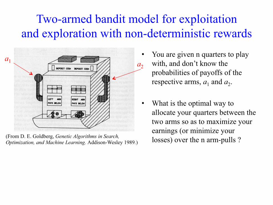
Two-armed bandit model for exploitation and exploration with non-deterministic rewards
• You are given n quarters to play with, and don’t know the probabilities of payoffs of the respective arms, a1 and a2.
• What is the optimal way to allocate your quarters between the two arms so as to maximize your earnings (or minimize your losses) over the n arm-pulls ? (From D. E. Goldberg, Genetic Algorithms in Search,
Optimization, and Machine Learning. Addison-Wesley 1989.)
a1 a2

• Each arm roughly corresponds with a possible “strategy” to test.
• The question is, how should you allocate the next sample between the two different arms, given what rewards you have obtained so far?
• Let Q(a) = expected reward of arm a.
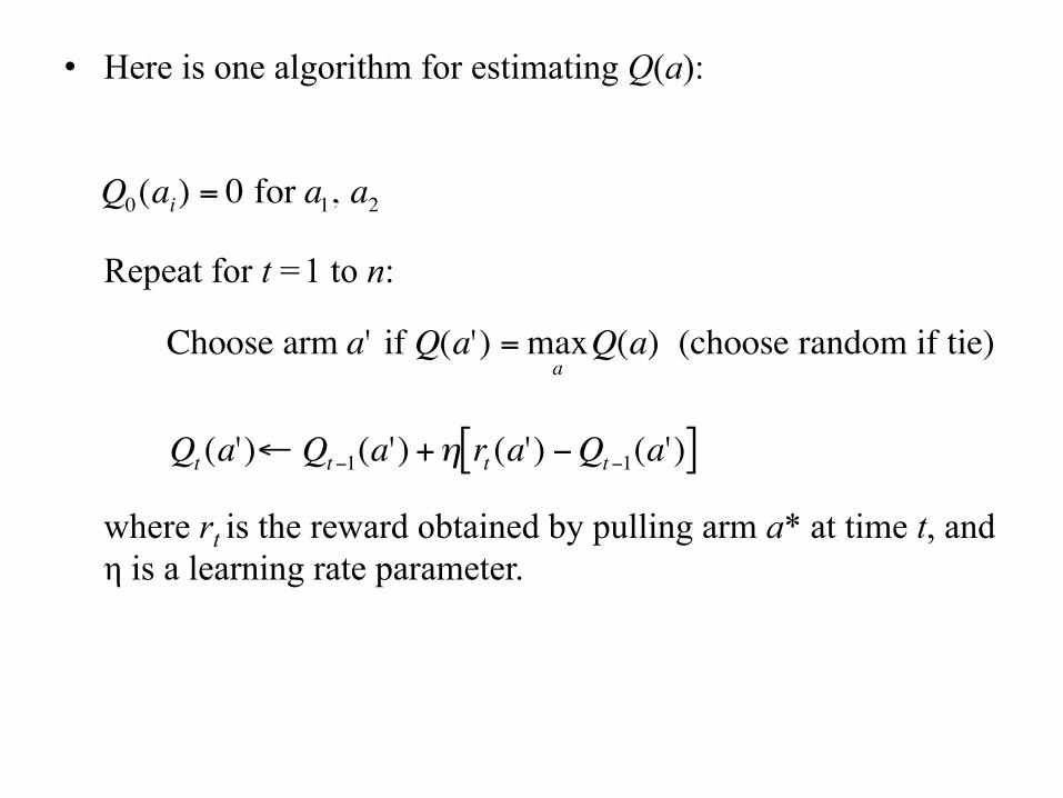
• Here is one algorithm for estimating Q(a):
Repeat for t =1 to n:
where rt is the reward obtained by pulling arm a* at time t, and η is a learning rate parameter.
€
Qt (a')← Qt−1(a') +η rt (a') −Qt−1(a')[ ]€
Choose arm a' if Q(a') = maxaQ(a) (choose random if tie)€
Q0(ai) = 0 for a1, a2

• Can generalize to “k-armed bandit”, where each arm is a possible “strategy”.
• This model was used in the development of reinforcement learning.
Applications of reinforcement learning: A few examples
• Learning to play backgammon
• Robot arm control (juggling)
• Robo-soccer
• Robot navigation
• Elevator dispatching
• Power systems stability control
• Job-shop scheduling
• Air traffic control

Robby the Robot can learn via reinforcement learning Sensors:
N, S, E, W, C(urrent) Actions:
Move N Move S Move E Move W Move random Stay put Try to pick up can
Rewards/Penalties (points):
Picks up can: 10 Tries to pick up can on empty site: -1 Crashes into wall: -5
“policy” = “strategy”
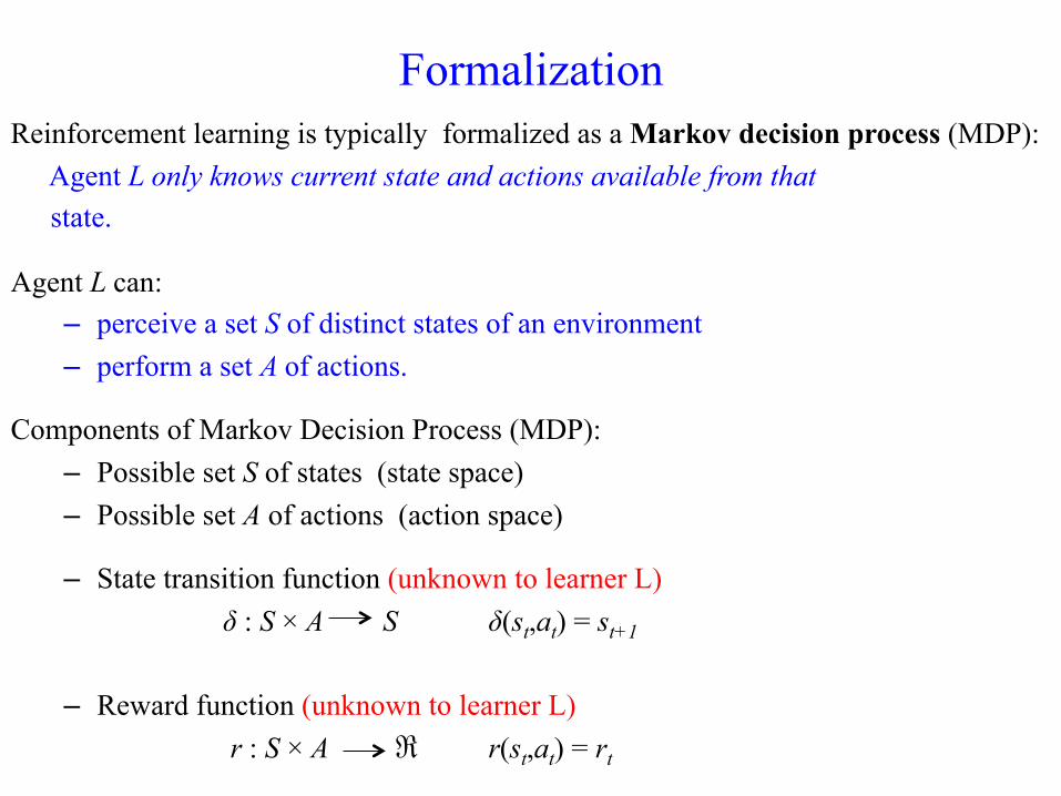
Formalization Reinforcement learning is typically formalized as a Markov decision process (MDP):
Agent L only knows current state and actions available from that state.
Agent L can: – perceive a set S of distinct states of an environment – perform a set A of actions.
Components of Markov Decision Process (MDP): – Possible set S of states (state space) – Possible set A of actions (action space)
– State transition function (unknown to learner L) δ : S × A S δ(st,at) = st+1
– Reward function (unknown to learner L) r : S × A ℜ r(st,at) = rt
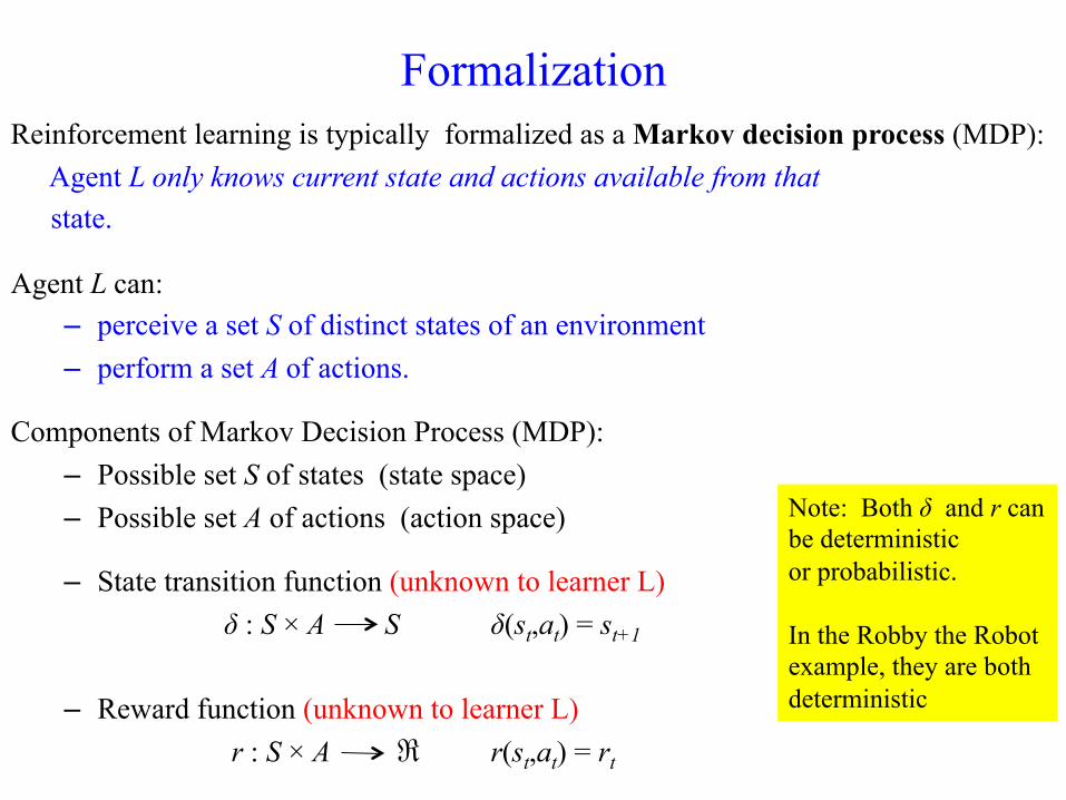
Note: Both δ and r can be deterministic or probabilistic. In the Robby the Robot example, they are both deterministic

Goal is for agent L to learn policy π, π : S A, such that π maximizes cumulative reward

Example: Cumulative value of a policy
Sensors: N,S,E,W,C(urrent)
Actions: Move N Move S Move E Move W Move random Stay put Try to pick up can
Rewards/Penalties (points):
Picks up can: 10 Tries to pick up can on empty site: -1 Crashes into wall: -5
Policy A: Always move east, picking up cans as you go Policy B: Move up and down the columns of the grid,
picking up cans as you go

Value function: Formal definition of “cumulative value” with discounted rewards
Let Vπ(st) denote the “cumulative value” of π starting from initial state st:
• where 0 ≤ γ ≤ 1 is a “discounting” constant that determines the relative value of delayed versus immediate rewards.
• Vπ(st) is called the “value function” for policy π . It gives the expected value of starting in state st and following policy π “forever”.
€
V π (st ) = rt +γ rt+1 +γ 2rt+2 + ...
= γ i
i=0
∞
∑ rt+ i

Value function: Formal definition of “cumulative value” with discounted rewards
Let Vπ(st) denote the “cumulative value” of π starting from initial state st:
• where 0 ≤ γ ≤ 1 is a “discounting” constant that determines the relative value of delayed versus immediate rewards.
• Vπ(st) is called the “value function” for policy π . It gives the expected value of starting in state st and following policy π “forever”.
€
V π (st ) = rt +γ rt+1 +γ 2rt+2 + ...
= γ i
i=0
∞
∑ rt+ i Why use a discounting constant?

• Note that rewards received i times steps into the future are discounted exponentially (by a factor of γi).
• If γ = 0, we only care about immediate reward.
• The closer γ is to 1, the more we care about future rewards, relative to immediate reward.

• Precise specification of learning task:
We require that the agent learn policy π that maximizes Vπ(s) for all states s.
We call such a policy an optimal policy, and denote it by π*:
To simplify notation, let
V *(s) =V π*(s)

What should L learn?
• Hard to learn π* directly, since we don’t have training data of the form (s, a)
• Only training data availale to learner is sequence of rewards: r(s0, a0), r(s1, a1), ...
• So, what should the learner L learn?

Learn evaluation function V?
• One possibility: learn evaluation function V*(s).
• Then L would know what action to take next:
– L should prefer state s1 over s2 whenever V*(s1) > V*(s2)
– Optimal action a in state s is the one that maximizes sum of r(s,a) (immediate reward) and V* of the immediate successor state, discounted by γ:
€
π * (s) = argmaxa
r(s,a) + γV * (δ(s,a))[ ]

€
π * (s) = argmaxa
r(s,a) + γV * (δ(s,a))[ ]

Problem with learning V*
Problem: Using V* to obtain optimal policy π* requires perfect knowledge of δ and r, which we earlier said are unknown to L.

Alternative: Q Learning
• Alternative: we will estimate the following evaluation function Q: S × A ℜ, as follows:
• Suppose learner L has a good estimate for Q(s,a). Then, at
each time step, L simply chooses action that maximizes Q(s,a).
€
π * (s) = argmaxa
r(s,a) + γV * (δ(s,a))[ ]
= argmaxa
Q(s,a)[ ],
where Q(s,a) = r(s,a) + γV * (δ(s,a))

How to learn Q ? (In theory)
We have: We can learn Q via iterative approximation. €
π * (s) = argmaxa '
r(s,a') + γV * (δ(s,a'))[ ]
V * (s) =maxa
r(s,a') + γV * (δ(s,a'))[ ]=max
a 'Q(s,a')[ ]
So,
Q(s,a) = r(s,a) + γmaxa '
Q(δ(s,a),a')[ ]

How to learn Q ? (In practice)
• Initialize Q(s,a) to small random values for all s and a
• Initialize s
• Repeat forever (or as long as you have time for): – Select action a – Take action a and receive reward r – Observe new state s´ – Update Q(s,a) ⇐ Q(s,a) + η (r + γ maxa´ Q(s´,a´) – Q(s, a))
– Update s ⇐ s´

Example of Q learning
Q(s,a) MoveN MoveS MoveE MoveW Move Random
Stay Put Pick Up Can
…
…
State: North, South, East, West, Current W = Wall E = Empty C = Can Reward:
Let γ = .2 Let η = 1

Example of Q learning
Q(s,a) MoveN MoveS MoveE MoveW Move Random
Stay Put Pick Up Can
… 0 0 0 0 0 0 0
0 0 0 0 0 0 0
0 0 0 0 0 0 0
0 0 0 0 0 0 0
… 0 0 0 0 0 0 0
State: North, South, East, West, Current W = Wall E = Empty C = Can Reward:
Ini;alize Q(s,a) to small random values (here, 0) for all s and a

Example of Q learning
Q(s,a) MoveN MoveS MoveE MoveW Move Random
Stay Put Pick Up Can
… 0 0 0 0 0 0 0
0 0 0 0 0 0 0
W, E, C, W, E 0 0 0 0 0 0 0
0 0 0 0 0 0 0
… 0 0 0 0 0 0 0
State: North, South, East, West, Current W = Wall E = Empty C = Can Reward:
Ini;alize s

Example of Q learning
Q(s,a) MoveN MoveS MoveE MoveW Move Random
Stay Put Pick Up Can
… 0 0 0 0 0 0 0
0 0 0 0 0 0 0
W, E, C, W, E 0 0 0 0 0 0 0
0 0 0 0 0 0 0
… 0 0 0 0 0 0 0
State: North, South, East, West, Current W = Wall E = Empty C = Can Reward:
Select ac;on a
Trial: 1

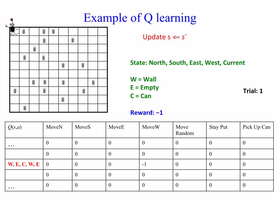
Example of Q learning
Q(s,a) MoveN MoveS MoveE MoveW Move Random
Stay Put Pick Up Can
… 0 0 0 0 0 0 0
0 0 0 0 0 0 0
W, E, C, W, E 0 0 0 0 0 0 0
0 0 0 0 0 0 0
… 0 0 0 0 0 0 0
State: North, South, East, West, Current W = Wall E = Empty C = Can Reward: −1
Perform ac;on a and receive reward r
Trial: 1

Example of Q learning
Q(s,a) MoveN MoveS MoveE MoveW Move Random
Stay Put Pick Up Can
… 0 0 0 0 0 0 0
0 0 0 0 0 0 0
W, E, C, W, E 0 0 0 0 0 0 0
0 0 0 0 0 0 0
… 0 0 0 0 0 0 0
State: North, South, East, West, Current W = Wall E = Empty C = Can Reward: −1
Observe new state s´
Trial: 1

Example of Q learning
Q(s,a) MoveN MoveS MoveE MoveW Move Random
Stay Put Pick Up Can
… 0 0 0 0 0 0 0
0 0 0 0 0 0 0
W, E, C, W, E 0 0 0 -1 0 0 0
0 0 0 0 0 0 0
… 0 0 0 0 0 0 0
State: North, South, East, West, Current W = Wall E = Empty C = Can Reward: −1
Update Q(s,a) ⇐ Q(s,a) + η (r + γ maxa´ Q(s´,a´) – Q(s, a))
Trial: 1
Example of Q learning
Q(s,a) MoveN MoveS MoveE MoveW Move Random
Stay Put Pick Up Can
… 0 0 0 0 0 0 0
0 0 0 0 0 0 0
W, E, C, W, E 0 0 0 -1 0 0 0
0 0 0 0 0 0 0
… 0 0 0 0 0 0 0
State: North, South, East, West, Current W = Wall E = Empty C = Can Reward: −1
Update s ⇐ s´
Trial: 1

Example of Q learning
Q(s,a) MoveN MoveS MoveE MoveW Move Random
Stay Put Pick Up Can
… 0 0 0 0 0 0 0
0 0 0 0 0 0 0
W, E, C, W, E 0 0 0 -1 0 0 0
0 0 0 0 0 0 0
… 0 0 0 0 0 0 0
State: North, South, East, West, Current W = Wall E = Empty C = Can Reward:
Select ac;on a
Trial: 2

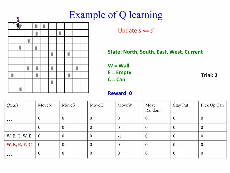
Example of Q learning
Q(s,a) MoveN MoveS MoveE MoveW Move Random
Stay Put Pick Up Can
… 0 0 0 0 0 0 0
0 0 0 0 0 0 0
W, E, C, W, E 0 0 0 -1 0 0 0
0 0 0 0 0 0 0
… 0 0 0 0 0 0 0
State: North, South, East, West, Current W = Wall E = Empty C = Can Reward: 0
Perform ac;on a and receive reward r
Trial: 2

Example of Q learning
Q(s,a) MoveN MoveS MoveE MoveW Move Random
Stay Put Pick Up Can
… 0 0 0 0 0 0 0
0 0 0 0 0 0 0
W, E, C, W, E 0 0 0 -1 0 0 0
W, E, E, E, C 0 0 0 0 0 0 0
… 0 0 0 0 0 0 0
State: North, South, East, West, Current W = Wall E = Empty C = Can Reward: 0
Observe new state s´
Trial: 2

Example of Q learning
Q(s,a) MoveN MoveS MoveE MoveW Move Random
Stay Put Pick Up Can
… 0 0 0 0 0 0 0
0 0 0 0 0 0 0
W, E, C, W, E 0 0 0 -1 0 0 0
W, E, E, E, C 0 0 0 0 0 0 0
… 0 0 0 0 0 0 0
State: North, South, East, West, Current W = Wall E = Empty C = Can Reward: 0
Trial: 2
Update Q(s,a) ⇐ Q(s,a) + η (r + γ maxa´ Q(s´,a´) – Q(s, a))
Example of Q learning
Q(s,a) MoveN MoveS MoveE MoveW Move Random
Stay Put Pick Up Can
… 0 0 0 0 0 0 0
0 0 0 0 0 0 0
W, E, C, W, E 0 0 0 -1 0 0 0
W, E, E, E, C 0 0 0 0 0 0 0
… 0 0 0 0 0 0 0
State: North, South, East, West, Current W = Wall E = Empty C = Can Reward: 0
Update s ⇐ s´
Trial: 2

Example of Q learning
Q(s,a) MoveN MoveS MoveE MoveW Move Random
Stay Put Pick Up Can
… 0 0 0 0 0 0 0
0 0 0 0 0 0 0
W, E, C, W, E 0 0 0 -1 0 0 0
W, E, E, E, C 0 0 0 0 0 0 0
… 0 0 0 0 0 0 0
State: North, South, East, West, Current W = Wall E = Empty C = Can Reward:
Select ac;on a
Trial: 3

Example of Q learning
Q(s,a) MoveN MoveS MoveE MoveW Move Random
Stay Put Pick Up Can
… 0 0 0 0 0 0 0
0 0 0 0 0 0 0
W, E, C, W, E 0 0 0 -1 0 0 0
W, E, E, E, C 0 0 0 0 0 0 0
… 0 0 0 0 0 0 0
State: North, South, East, West, Current W = Wall E = Empty C = Can Reward: 10
Perform ac;on a and receive reward r
Trial: 3
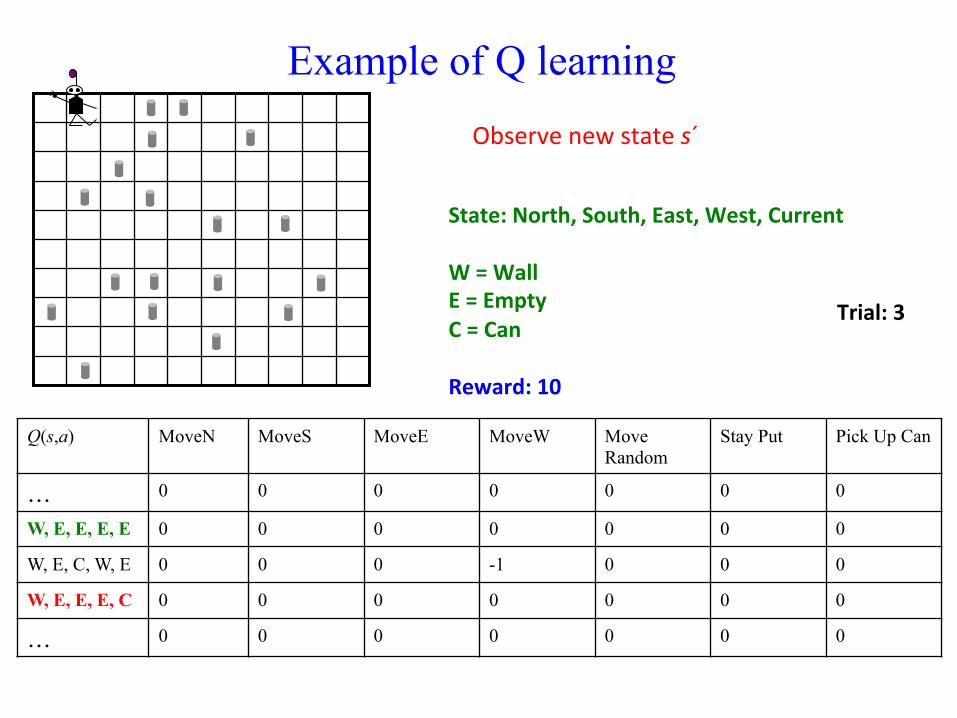
Example of Q learning
Q(s,a) MoveN MoveS MoveE MoveW Move Random
Stay Put Pick Up Can
… 0 0 0 0 0 0 0
W, E, E, E, E 0 0 0 0 0 0 0
W, E, C, W, E 0 0 0 -1 0 0 0
W, E, E, E, C 0 0 0 0 0 0 0
… 0 0 0 0 0 0 0
State: North, South, East, West, Current W = Wall E = Empty C = Can Reward: 10
Observe new state s´
Trial: 3

Example of Q learning
State: North, South, East, West, Current W = Wall E = Empty C = Can Reward: 10
Trial: 3
Update Q(s,a) ⇐ Q(s,a) + η (r + γ maxa´ Q(s´,a´) – Q(s, a))
Q(s,a) MoveN MoveS MoveE MoveW Move Random
Stay Put Pick Up Can
… 0 0 0 0 0 0 0
W, E, E, E, E 0 0 0 0 0 0 0
W, E, C, W, E 0 0 0 -1 0 0 0
W, E, E, E, C 0 0 0 0 0 0 10
… 0 0 0 0 0 0 0

Example of Q learning
State: North, South, East, West, Current W = Wall E = Empty C = Can Reward: 10
Update s ⇐ s´
Trial: 3
Q(s,a) MoveN MoveS MoveE MoveW Move Random
Stay Put Pick Up Can
… 0 0 0 0 0 0 0
W, E, E, E, E 0 0 0 0 0 0 0
W, E, C, W, E 0 0 0 -1 0 0 0
W, E, E, E, C 0 0 0 0 0 0 10
… 0 0 0 0 0 0 0

Skipping ahead...
State: North, South, East, West, Current W = Wall E = Empty C = Can Reward:
Select ac;on a
Trial: m
Q(s,a) MoveN MoveS MoveE MoveW Move Random
Stay Put Pick Up Can
… 0 0 0 0 0 0 0
W, E, E, E, E 0 0 0 0 0 0 0
W, E, C, W, E 0 0 0 -1 0 0 0
W, E, E, E, C 0 0 0 0 0 0 10
… 0 0 0 0 0 0 0

Skipping ahead...
State: North, South, East, West, Current W = Wall E = Empty C = Can Reward: 10
Trial: m
Q(s,a) MoveN MoveS MoveE MoveW Move Random
Stay Put Pick Up Can
… 0 0 0 0 0 0 0
W, E, E, E, E 0 0 0 0 0 0 0
W, E, C, W, E 0 0 0 -1 0 0 0
W, E, E, E, C 0 0 0 0 0 0 10
… 0 0 0 0 0 0 0
Perform ac;on a and receive reward r

Skipping ahead...
State: North, South, East, West, Current W = Wall E = Empty C = Can Reward: 10
Trial: m
Q(s,a) MoveN MoveS MoveE MoveW Move Random
Stay Put Pick Up Can
… 0 0 0 0 0 0 0
W, E, E, E, E 0 0 0 0 0 0 0
W, E, C, W, E 0 0 0 -1 0 0 0
W, E, E, E, C 0 0 0 0 0 0 10
… 0 0 0 0 0 0 0
Observe new state s´

Skipping ahead...
State: North, South, East, West, Current W = Wall E = Empty C = Can Reward: 10
Trial: m
Q(s,a) MoveN MoveS MoveE MoveW Move Random
Stay Put Pick Up Can
… 0 0 0 0 0 0 0
W, E, E, E, E 0 0 0 0 0 0 0
W, E, C, W, E 0 0 0 -1 0 0 0
W, E, E, E, C 0 0 0 0 0 0 10
… 0 0 0 0 0 0 0
Update Q(s,a) ⇐ Q(s,a) + η (r + γ maxa´ Q(s´,a´) – Q(s, a))

Now on a new environment...
State: North, South, East, West, Current W = Wall E = Empty C = Can Reward:
Trial: n
Q(s,a) MoveN MoveS MoveE MoveW Move Random
Stay Put Pick Up Can
… 0 0 0 0 0 0 0
W, E, E, E, E 0 0 0 0 0 0 0
W, E, C, W, E 0 0 0 -1 0 0 0
W, E, E, E, C 0 0 0 0 0 0 10
… 0 0 0 0 0 0 0
Select ac;on a

Now on a new environment...
State: North, South, East, West, Current W = Wall E = Empty C = Can Reward: 0
Trial: n
Q(s,a) MoveN MoveS MoveE MoveW Move Random
Stay Put Pick Up Can
… 0 0 0 0 0 0 0
W, E, E, E, E 0 0 0 0 0 0 0
W, E, C, W, E 0 0 0 -1 0 0 0
W, E, E, E, C 0 0 0 0 0 0 10
… 0 0 0 0 0 0 0
Perform ac;on a and receive reward r

Now on a new environment...
State: North, South, East, West, Current W = Wall E = Empty C = Can Reward: 0
Trial: n
Q(s,a) MoveN MoveS MoveE MoveW Move Random
Stay Put Pick Up Can
… 0 0 0 0 0 0 0
W, E, E, E, E 0 0 0 0 0 0 0
W, E, C, W, E 0 0 0 -1 0 0 0
W, E, E, E, C 0 0 0 0 0 0 10
… 0 0 0 0 0 0 0
Observe new state s´

Now on a new environment...
State: North, South, East, West, Current W = Wall E = Empty C = Can Reward: 0
Trial: n
Q(s,a) MoveN MoveS MoveE MoveW Move Random
Stay Put Pick Up Can
… 0 0 0 0 0 0 0
W, E, E, E, E 0 0 0 0 0 0 0
W, E, C, W, E 0 0 2 -1 0 0 0
W, E, E, E, C 0 0 0 0 0 0 10
… 0 0 0 0 0 0 0
Update Q(s,a) ⇐ Q(s,a) + η (r + γ maxa´ Q(s´,a´) – Q(s, a))

How to choose actions?

How to choose actions?
• Naïve strategy: at each time step, choose action that maximizes Q(s,a)
How to choose actions?
• Naïve strategy: at each time step, choose action that maximizes Q(s,a)
• This exploits current Q but doesn’t further explore the state-action space (in case Q is way off)

How to choose actions?
• Naïve strategy: at each time step, choose action that maximizes Q(s,a)
• This exploits current Q but doesn’t further explore the state-action space (in case Q is way off)
• Common in Q learning to use probabilistic approach, e.g.,
€
P(ai | s) =eQ(s,ai ) /T
eQ(s,ai ) /Tj∑
, T > 0
• This balances exploitation and exploration in a tunable way: – high T: more exploration (more random) – low T: more exploitation (more deterministic)
• Can start with high T, and decrease it as improves

Representation of Q(s, a)
• Note that in all of the above discussion, Q(s, a) was assumed to be a look-up table, with a distinct table entry for each distinct (s,a) pair.
• More commonly, Q(s, a) is represented as a function (e.g., as a neural network), and the function is estimated (e.g., through back-propagation).

Example: Learning to play backgammon
Rules of backgammon

Complexity of Backgammon
• Over 1020 possible states.
• At each ply, 21 dice combinations, with average of about 20 legal moves per dice combination. Result is branching ratio of several hundred per ply.
• Chess has branching ratio of about 30-40 per ply.
• Brute-force look-ahead search is not practical!

Neurogammon (Tesauro, 1989)
• Used supervised learning approach: multilayer NN trained by back-propagation on data base of recorded expert games.
• Input: raw board information (number of pieces at each location), and a few hand-crafted features that encoded important expert concepts.
• Neurogammon achieved strong intermediate level of play.
• Won backgammon championship at 1989 International Computer Olympiad. But not close to beating best human players.

TD-Gammon (G. Tesauro, 1994)
• Program had two main parts:
– Move Generator: Program that generates all legal moves from current board configuration.
– Predictor network: multi-layer NN that predicts Q(s,a): probability of winning the game from the current board configuration.
• Predictor network scores all legal moves. Highest scoring move is chosen.
• Rewards: Zero for all time steps except those on which game is won or lost.


• Input: 198 units – 24 positions, 8 input units for each position (192 input units) • First 4 input units of each group of 8 represent # white
pieces at that position, • Second 4 represent # black units at that position
– Two inputs represent who is moving (white or black)
– Two inputs represent pieces on the bar
– Two inputs represent number of pieces borne off by each player.

• 50 hidden units
• 1 output unit (activation represents probability that white will win from given board configuration)

Program plays against itself.
On each turn: • Use network to evaluate all possible moves from current board
configuration. Choose the move with the highest (lowest as black) evaluation. This produces a new board configuration.
• If this is end of game, run back-propagation, with target output activation of 1 or 0 depending on whether white won or lost.
• Else evaluate new board configuration with neural network. Calculate difference between current evaluation and previous evaluation.
• Run back-propagation, using the current evaluation as desired output, and the board position previous to the current move as the input.


• From Sutton & Barto, Reinforcement Learning: An Introduction:
“After playing about 300,000 games against itself, TD-Gammon 0.0 as described above learned to play approximately as well as the best previous backgammon computer programs.”
“TD-Gammon 3.0 appears to be at, or very near, the playing strength of the best human players in the world. It may already be the world champion. These programs have already changed the way the best human players play the game. For example, TD-Gammon learned to play certain opening positions differently than was the convention among the best human players. Based on TD-Gammon's success and further analysis, the best human players now play these positions as TD-Gammon does (Tesauro, 1995).”

Applying RL to Robotics
Robosoccer with RL-Decision-tree learning: http://www.youtube.com/watch?v=mRpX9DFCdwI
Robo pancake flipper http://www.youtube.com/watch?v=W_gxLKSsSIE


![[DL Hacks輪読] Semi-Supervised Learning with Ladder Networks (NIPS2015)](https://img.pdfslide.tips/doc/110x75/587f4b801a28ab43318b76ab/dl-hacks-semi-supervised-learning-with-ladder-networks-nips2015.jpg)