An Overview of Deep Semi-Supervised Learning

Yassine Ouali �∗ Céline Hudelot Myriam TamiUniversité Paris-Saclay, CentraleSupélec, MICS, 91190, Gif-sur-Yvette, France

{yassine.ouali,celine.hudelot,myriam.tami}@centralesupelec.fr

Abstract

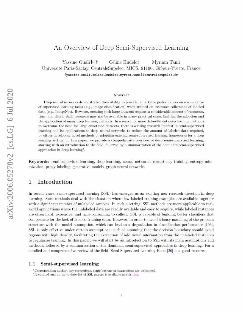
Deep neural networks demonstrated their ability to provide remarkable performances on a wide rangeof supervised learning tasks (e.g., image classification) when trained on extensive collections of labeleddata (e.g., ImageNet). However, creating such large datasets requires a considerable amount of resources,time, and effort. Such resources may not be available in many practical cases, limiting the adoption andthe application of many deep learning methods. In a search for more data-efficient deep learning methodsto overcome the need for large annotated datasets, there is a rising research interest in semi-supervisedlearning and its applications to deep neural networks to reduce the amount of labeled data required,by either developing novel methods or adopting existing semi-supervised learning frameworks for a deeplearning setting. In this paper, we provide a comprehensive overview of deep semi-supervised learning,starting with an introduction to the field, followed by a summarization of the dominant semi-supervisedapproaches in deep learning1.

Keywords: semi-supervised learning, deep learning, neural networks, consistency training, entropy mini-mization, proxy labeling, generative models, graph neural networks.

1 Introduction

In recent years, semi-supervised learning (SSL) has emerged as an exciting new research direction in deeplearning. Such methods deal with the situation where few labeled training examples are available togetherwith a significant number of unlabeled samples. In such a setting, SSL methods are more applicable to real-world applications where the unlabeled data are readily available and easy to acquire, while labeled instancesare often hard, expensive, and time-consuming to collect. SSL is capable of building better classifiers thatcompensate for the lack of labeled training data. However, in order to avoid a lousy matching of the problemstructure with the model assumption, which can lead to a degradation in classification performance [193],SSL is only effective under certain assumptions, such as assuming that the decision boundary should avoidregions with high density, facilitating the extraction of additional information from the unlabeled instancesto regularize training. In this paper, we will start by an introduction to SSL with its main assumptions andmethods, followed by a summarization of the dominant semi-supervised approaches in deep learning. For adetailed and comprehensive review of the field, Semi-Supervised Learning Book [20] is a good resource.

1.1 Semi-supervised learning∗Corresponding author, any corrections, contributions or suggestions are welcomed.1A curated and an up-to-date list of SSL papers is available at this link.

1

arX

iv:2

006.

0527

8v2

[cs

.LG

] 6

Jul

202

0

-ModelPseudo-Labeling VATEntropy MinimizationSupervised

Class A Class B Unlabeled

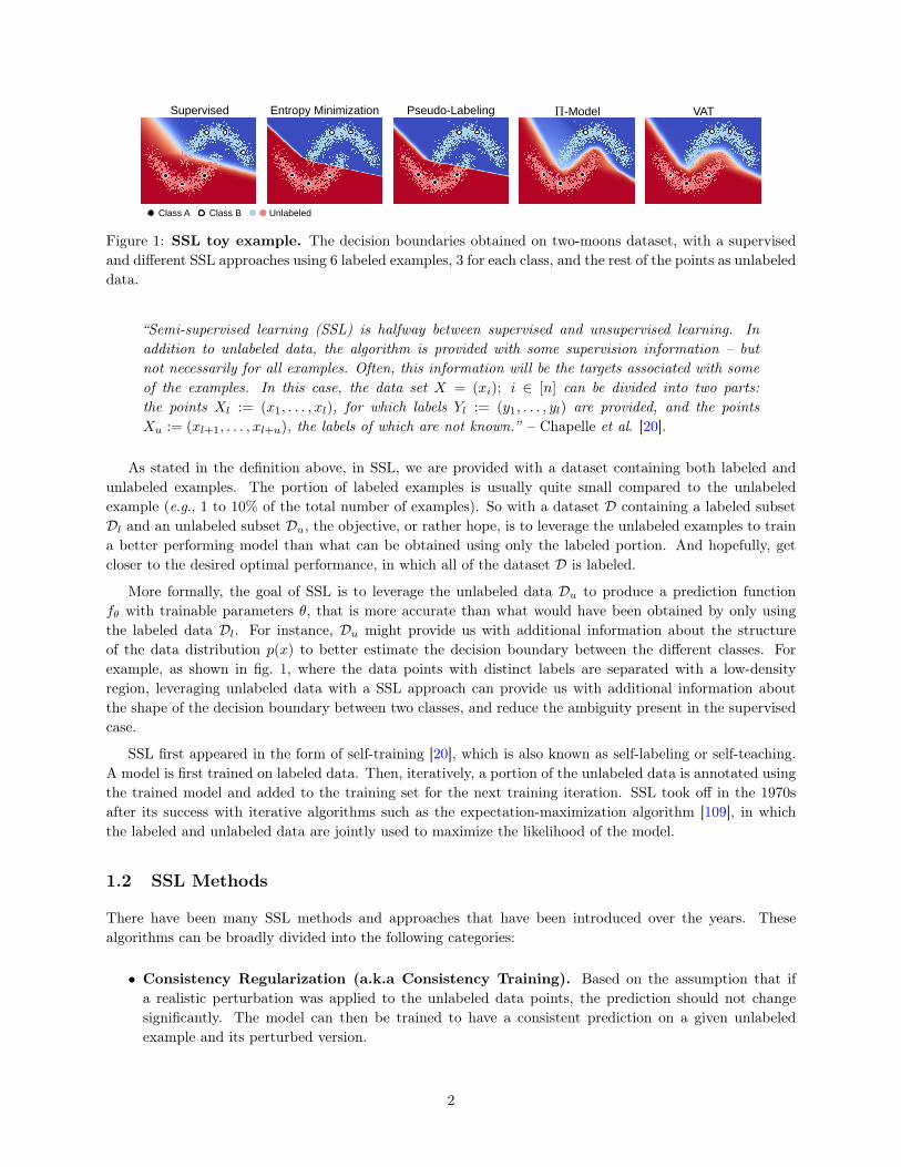
Figure 1: SSL toy example. The decision boundaries obtained on two-moons dataset, with a supervisedand different SSL approaches using 6 labeled examples, 3 for each class, and the rest of the points as unlabeleddata.

“Semi-supervised learning (SSL) is halfway between supervised and unsupervised learning. Inaddition to unlabeled data, the algorithm is provided with some supervision information – butnot necessarily for all examples. Often, this information will be the targets associated with someof the examples. In this case, the data set X = (xi); i ∈ [n] can be divided into two parts:the points Xl := (x1, . . . , xl), for which labels Yl := (y1, . . . , yl) are provided, and the pointsXu := (xl+1, . . . , xl+u), the labels of which are not known.” – Chapelle et al. [20].

As stated in the definition above, in SSL, we are provided with a dataset containing both labeled andunlabeled examples. The portion of labeled examples is usually quite small compared to the unlabeledexample (e.g., 1 to 10% of the total number of examples). So with a dataset D containing a labeled subsetDl and an unlabeled subset Du, the objective, or rather hope, is to leverage the unlabeled examples to traina better performing model than what can be obtained using only the labeled portion. And hopefully, getcloser to the desired optimal performance, in which all of the dataset D is labeled.

More formally, the goal of SSL is to leverage the unlabeled data Du to produce a prediction functionfθ with trainable parameters θ, that is more accurate than what would have been obtained by only usingthe labeled data Dl. For instance, Du might provide us with additional information about the structureof the data distribution p(x) to better estimate the decision boundary between the different classes. Forexample, as shown in fig. 1, where the data points with distinct labels are separated with a low-densityregion, leveraging unlabeled data with a SSL approach can provide us with additional information aboutthe shape of the decision boundary between two classes, and reduce the ambiguity present in the supervisedcase.

SSL first appeared in the form of self-training [20], which is also known as self-labeling or self-teaching.A model is first trained on labeled data. Then, iteratively, a portion of the unlabeled data is annotated usingthe trained model and added to the training set for the next training iteration. SSL took off in the 1970safter its success with iterative algorithms such as the expectation-maximization algorithm [109], in whichthe labeled and unlabeled data are jointly used to maximize the likelihood of the model.

1.2 SSL Methods

There have been many SSL methods and approaches that have been introduced over the years. Thesealgorithms can be broadly divided into the following categories:

• Consistency Regularization (a.k.a Consistency Training). Based on the assumption that ifa realistic perturbation was applied to the unlabeled data points, the prediction should not changesignificantly. The model can then be trained to have a consistent prediction on a given unlabeledexample and its perturbed version.

2

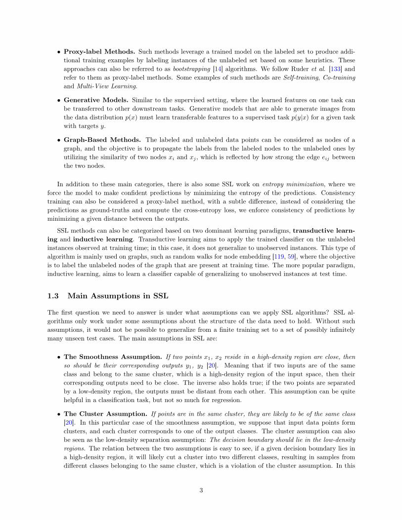
• Proxy-label Methods. Such methods leverage a trained model on the labeled set to produce addi-tional training examples by labeling instances of the unlabeled set based on some heuristics. Theseapproaches can also be referred to as bootstrapping [14] algorithms. We follow Ruder et al. [133] andrefer to them as proxy-label methods. Some examples of such methods are Self-training, Co-trainingand Multi-View Learning.

• Generative Models. Similar to the supervised setting, where the learned features on one task canbe transferred to other downstream tasks. Generative models that are able to generate images fromthe data distribution p(x) must learn transferable features to a supervised task p(y|x) for a given taskwith targets y.

• Graph-Based Methods. The labeled and unlabeled data points can be considered as nodes of agraph, and the objective is to propagate the labels from the labeled nodes to the unlabeled ones byutilizing the similarity of two nodes xi and xj , which is reflected by how strong the edge eij betweenthe two nodes.

In addition to these main categories, there is also some SSL work on entropy minimization, where weforce the model to make confident predictions by minimizing the entropy of the predictions. Consistencytraining can also be considered a proxy-label method, with a subtle difference, instead of considering thepredictions as ground-truths and compute the cross-entropy loss, we enforce consistency of predictions byminimizing a given distance between the outputs.

SSL methods can also be categorized based on two dominant learning paradigms, transductive learn-ing and inductive learning. Transductive learning aims to apply the trained classifier on the unlabeledinstances observed at training time; in this case, it does not generalize to unobserved instances. This type ofalgorithm is mainly used on graphs, such as random walks for node embedding [119, 59], where the objectiveis to label the unlabeled nodes of the graph that are present at training time. The more popular paradigm,inductive learning, aims to learn a classifier capable of generalizing to unobserved instances at test time.

1.3 Main Assumptions in SSL

The first question we need to answer is under what assumptions can we apply SSL algorithms? SSL al-gorithms only work under some assumptions about the structure of the data need to hold. Without suchassumptions, it would not be possible to generalize from a finite training set to a set of possibly infinitelymany unseen test cases. The main assumptions in SSL are:

• The Smoothness Assumption. If two points x1, x2 reside in a high-density region are close, thenso should be their corresponding outputs y1, y2 [20]. Meaning that if two inputs are of the sameclass and belong to the same cluster, which is a high-density region of the input space, then theircorresponding outputs need to be close. The inverse also holds true; if the two points are separatedby a low-density region, the outputs must be distant from each other. This assumption can be quitehelpful in a classification task, but not so much for regression.

• The Cluster Assumption. If points are in the same cluster, they are likely to be of the same class[20]. In this particular case of the smoothness assumption, we suppose that input data points formclusters, and each cluster corresponds to one of the output classes. The cluster assumption can alsobe seen as the low-density separation assumption: The decision boundary should lie in the low-densityregions. The relation between the two assumptions is easy to see, if a given decision boundary lies ina high-density region, it will likely cut a cluster into two different classes, resulting in samples fromdifferent classes belonging to the same cluster, which is a violation of the cluster assumption. In this

3

case, we can restrict our model to have consistent predictions on the unlabeled data over some smallperturbations pushing its decision boundary to low-density regions.

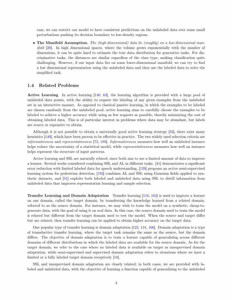
• The Manifold Assumption. The (high-dimensional) data lie (roughly) on a low-dimensional man-ifold [20]. In high dimensional spaces, where the volume grows exponentially with the number ofdimensions, it can be quite hard to estimate the true data distribution for generative tasks. For dis-criminative tasks, the distances are similar regardless of the class type, making classification quitechallenging. However, if our input data lies on some lower-dimensional manifold, we can try to finda low dimensional representation using the unlabeled data and then use the labeled data to solve thesimplified task.

1.4 Related Problems

Active Learning In active learning [140, 63], the learning algorithm is provided with a large pool ofunlabeled data points, with the ability to request the labeling of any given examples from the unlabeledset in an interactive manner. As opposed to classical passive learning, in which the examples to be labeledare chosen randomly from the unlabeled pool, active learning aims to carefully choose the examples to belabeled to achieve a higher accuracy while using as few requests as possible, thereby minimizing the cost ofobtaining labeled data. This is of particular interest in problems where data may be abundant, but labelsare scarce or expensive to obtain.

Although it is not possible to obtain a universally good active learning strategy [33], there exist manyheuristics [140], which have been proven to be effective in practice. The two widely used selection criteria areinformativeness and representativeness [72, 188]. Informativeness measures how well an unlabeled instancehelps reduce the uncertainty of a statistical model, while representativeness measures how well an instancehelps represent the structure of input patterns.

Active learning and SSL are naturally related, since both aim to use a limited amount of data to improvea learner. Several works considered combining SSL and AL in different tasks. [41] demonstrates a significanterror reduction with limited labeled data for speech understanding, [129] proposes an active semi-supervisedlearning system for pedestrian detection, [192] combines AL and SSL using Gaussian fields applied to syn-thetic datasets, and [51] exploits both labeled and unlabeled data using SSL to distill information fromunlabeled data that improves representation learning and sample selection.

Transfer Learning and Domain Adaptation Transfer learning [116, 162] is used to improve a learneron one domain, called the target domain, by transferring the knowledge learned from a related domain,referred to as the source domain. For instance, we may wish to train the model on a synthetic, cheap-to-generate data, with the goal of using it on real data. In this case, the source domain used to train the modelis related but different from the target domain used to test the model. When the source and target differbut are related, then transfer learning can be applied to obtain higher accuracy on the target data.

One popular type of transfer learning is domain adaptation [122, 118, 166]. Domain adaptation is a typeof transductive transfer learning, where the target task remains the same as the source, but the domaindiffers. The objective of domain adaptation is to train a learner capable of generalizing across differentdomains of different distributions in which the labeled data are available for the source domain. As for thetarget domain, we refer to the case where no labeled data is available on target as unsupervised domainadaptation, while semi-supervised and supervised domain adaptation refers to situations where we have alimited or a fully labeled target domain receptively [10].

SSL and unsupervised domain adaptation are closely related; in both cases, we are provided with la-beled and unlabeled data, with the objective of learning a function capable of generalizing to the unlabeled

4

data and unseen examples. However, in SSL, both the labeled and unlabeled sets come from the samedistribution, while in unsupervised domain adaptation, the target and source distributions differ. Methodsin both subjects can be leveraged interchangeably. In SSL, [104] proposed to use adversarial distributionalignment [50] for semi-supervised image classification using only a small amount of labeled samples. As forunsupervised domain adaptation, semi-supervised methods, such as consistency regularization [142, 95, 47],co-regularization [91] or proxy labeling [134, 133] demonstrated their effectiveness in domain adaptation.

Weakly-Supervised Learning To overcome the need for large hand-labeled and expensive training sets,most sizeable deep learning systems use some form of weak supervision: lower-quality, but larger-scaletraining sets constructed via strategies such as using cheap annotators [126]. In weakly-supervised learning,the objective is the same as in supervised learning, however, instead of a ground-truth labeled trainingset, we are provided with one or more weakly annotated examples, that could come from crowd workers,be the output of heuristic rules, the result of distant supervision [106], or the output of other classifiers.For example, in weakly-supervised semantic segmentation, pixel-level labels, which are harder and moreexpensive to acquire, are substituted for inexact annotations, e.g., image labels [159, 184, 161, 97, 94], points[9], scribbles [100] and bounding boxes [144, 31]. In such a scenario, SSL approaches can be used to enhancethe performance further if a limited number of strongly labeled examples are available while still takingadvantage of the weakly labeled examples.

Learning with Noisy Labels Learning from noisy labels [46, 52] can be challenging given the negativeimpact label noise can have on the performance of deep learning methods if the noise is significant. Toovercome this, most existing methods for training deep neural networks with noisy labels seek to correct theloss function. One type of correction consists of treating all the examples as equal and relabeling the noisyexamples, where proxy labels methods can be used for the relabeling procedure [174, 101, 127]. Anothertype of correction applies a reweighing to the training examples to distinguish between the clean and noisysamples [28, 149]. Other works [35, 69, 87, 96] have shown that SSL can be useful in learning from noisylabels, where the noisy labels are discarded, and the noisy examples are considered as unlabeled data andused to regularize training using SSL methods.

1.5 Evaluating SSL Approaches

The conventional experimental procedure used to evaluate SSL methods consists of choosing a dataset (e.g.,CIFAR-10 [88], SVHN [110], ImageNet [34], IMDb [103], Yelp review [180]) commonly used for supervisedlearning, a large portion of the labels are then ignored, resulting in a small labeled set Dl and a largerunlabeled Du. A deep learning model is trained with a given SSL approach, and the results are reportedon the original test set over various and standardized portions of labeled examples. In order to make thisprocedure applicable to real-world settings, Oliver et al. [113] proposed the following ways to improve thisexperimental methodology:

• A Shared Implementation. For a realistic comparison of different SSL methods, they must sharethe same underlying architectures and other implementation details (e.g., hyperparameters, parameterinitialization, data augmentation, regularization, etc.).

• High-Quality Supervised Baseline. The main objective of SSL is to obtain better performancethan what can be obtained in a supervised manner. This is why it is essential to provide a strongbaseline consisting of training the same model on the labeled set Dl in a supervised way, with modifiedhyperparameters to report the best-case performance of the fully-supervised model.

5

• Comparison to Transfer Learning. Another robust baseline to compare SSL methods to can beobtained by training the model on large labeled datasets, and then fine-tune it on the small labeledset Dl.

• Considering Class Distribution Mismatch. The possible distribution mismatch between thelabeled and unlabeled examples can be ignored when doing evaluation since both sets come from thesame dataset. Still, such a mismatch is prevalent in real-world applications, where the unlabeled datacan have different class distributions compared to the labeled data. The effect of this discrepancy needsto be addressed for better real-world adoption of SSL.

• Varying the Amount of Labeled and Unlabeled Data. A common practice in SSL is varyingthe number of labeled examples, but also varying the size Du in a systematic way to simulate realisticscenarios, such as training on a relatively small unlabeled set, can provide additional insights into theeffectiveness of SSL approaches.

• Realistically Small Validation Sets. In many cases where a fully annotated dataset if used forevaluation, we might end-up with a validation set that is significantly larger than the labeled set Dlused for training, in such a setting, extensive hyperparameter tuning might result in an overfitting tothe validation set. In contrast, small validation sets constrain the ability to select models [20, 45],resulting in a more realistic assessment of the performance of SSL methods.

2 Consistency Regularization

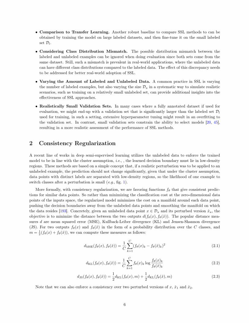
A recent line of works in deep semi-supervised learning utilizes the unlabeled data to enforce the trainedmodel to be in line with the cluster assumption, i.e., , the learned decision boundary must lie in low-densityregions. These methods are based on a simple concept that, if a realistic perturbation was to be applied to anunlabeled example, the prediction should not change significantly, given that under the cluster assumption,data points with distinct labels are separated with low-density regions, so the likelihood of one example toswitch classes after a perturbation is small (e.g., fig. 1).

More formally, with consistency regularization, we are favoring functions fθ that give consistent predic-tions for similar data points. So rather than minimizing the classification cost at the zero-dimensional datapoints of the inputs space, the regularized model minimizes the cost on a manifold around each data point,pushing the decision boundaries away from the unlabeled data points and smoothing the manifold on whichthe data resides [193]. Concretely, given an unlabeled data point x ∈ Du and its perturbed version xu, theobjective is to minimize the distance between the two outputs d(fθ(x), fθ(x)). The popular distance mea-sures d are mean squared error (MSE), Kullback-Leiber divergence (KL) and Jensen-Shannon divergence(JS). For two outputs fθ(x) and fθ(x) in the form of a probability distribution over the C classes, andm = 1

2 (fθ(x) + fθ(x)), we can compute these measures as follows:

dMSE(fθ(x), fθ(x)) =1

C

C∑k=1

(fθ(x)k − fθ(x)k)2 (2.1)

dKL(fθ(x), fθ(x)) =1

C

C∑k=1

fθ(x)k logfθ(x)kfθ(x)k

(2.2)

dJS(fθ(x), fθ(x)) =1

2dKL(fθ(x),m) +

1

2dKL(fθ(x),m) (2.3)

Note that we can also enforce a consistency over two perturbed versions of x, x1 and x2.

6

Denoising Decoder

Encoder

Noisy Encoder

Gaussian Noise

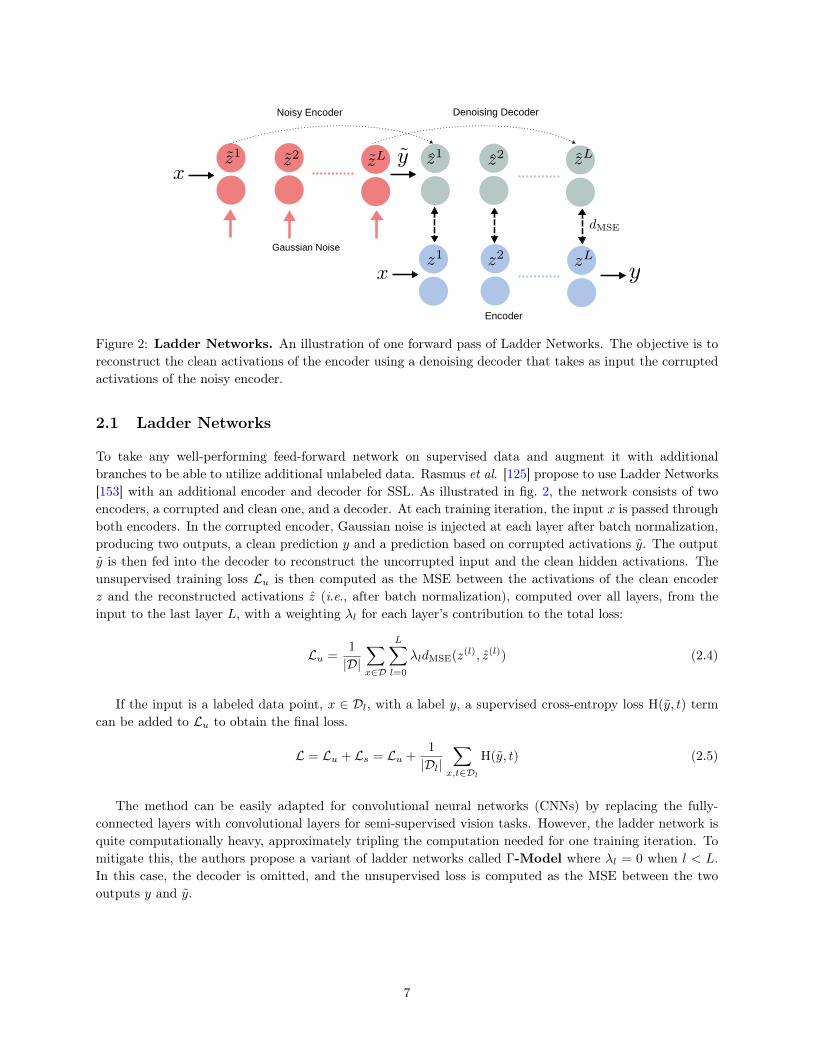
Figure 2: Ladder Networks. An illustration of one forward pass of Ladder Networks. The objective is toreconstruct the clean activations of the encoder using a denoising decoder that takes as input the corruptedactivations of the noisy encoder.

2.1 Ladder Networks

To take any well-performing feed-forward network on supervised data and augment it with additionalbranches to be able to utilize additional unlabeled data. Rasmus et al. [125] propose to use Ladder Networks[153] with an additional encoder and decoder for SSL. As illustrated in fig. 2, the network consists of twoencoders, a corrupted and clean one, and a decoder. At each training iteration, the input x is passed throughboth encoders. In the corrupted encoder, Gaussian noise is injected at each layer after batch normalization,producing two outputs, a clean prediction y and a prediction based on corrupted activations y. The outputy is then fed into the decoder to reconstruct the uncorrupted input and the clean hidden activations. Theunsupervised training loss Lu is then computed as the MSE between the activations of the clean encoderz and the reconstructed activations z (i.e., after batch normalization), computed over all layers, from theinput to the last layer L, with a weighting λl for each layer’s contribution to the total loss:

Lu =1

|D|∑x∈D

L∑l=0

λldMSE(z(l), z(l)) (2.4)

If the input is a labeled data point, x ∈ Dl, with a label y, a supervised cross-entropy loss H(y, t) termcan be added to Lu to obtain the final loss.

L = Lu + Ls = Lu +1

|Dl|∑x,t∈Dl

H(y, t) (2.5)

The method can be easily adapted for convolutional neural networks (CNNs) by replacing the fully-connected layers with convolutional layers for semi-supervised vision tasks. However, the ladder network isquite computationally heavy, approximately tripling the computation needed for one training iteration. Tomitigate this, the authors propose a variant of ladder networks called Γ-Model where λl = 0 when l < L.In this case, the decoder is omitted, and the unsupervised loss is computed as the MSE between the twooutputs y and y.

7

Networkwith dropout

Augmentations

CrossEntropy

Loss

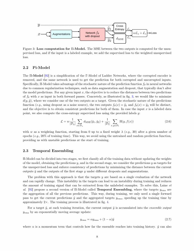
Figure 3: Loss computation for Π-Model. The MSE between the two outputs is computed for the unsu-pervised loss, and if the input is a labeled example, we add the supervised loss to the weighted unsupervisedloss.

2.2 Pi-Model

The Π-Model [92] is a simplification of the Γ-Model of Ladder Networks, where the corrupted encoder isremoved, and the same network is used to get the prediction for both corrupted and uncorrupted inputs.Specifically, Π-Model takes advantage of the stochastic nature of the prediction function fθ in neural networksdue to common regularization techniques, such as data augmentation and dropout, that typically don’t alterthe model predictions. For any given input x, the objective is to reduce the distances between two predictionsof fθ with x as input in both forward passes. Concretely, as illustrated in fig. 3, we would like to minimized(y, y), where we consider one of the two outputs as a target. Given the stochastic nature of the predictionsfunction (e.g., using dropout as a noise source), the two outputs fθ(x) = y1 and fθ(x) = y2 will be distinct,and the objective is to obtain consistent predictions for both of them. In case the input x is a labeled datapoint, we also compute the cross-entropy supervised loss using the provided labels y:

L = w1

|Du|∑x∈Du

dMSE(y1, y2) +1

|Dl|∑

x,y∈Dl

H(y, f(x)) (2.6)

with w as a weighting function, starting from 0 up to a fixed weight λ (e.g., 30) after a given number ofepochs (e.g., 20% of training time). This way, we avoid using the untrained and random prediction function,providing us with unstable predictions at the start of training.

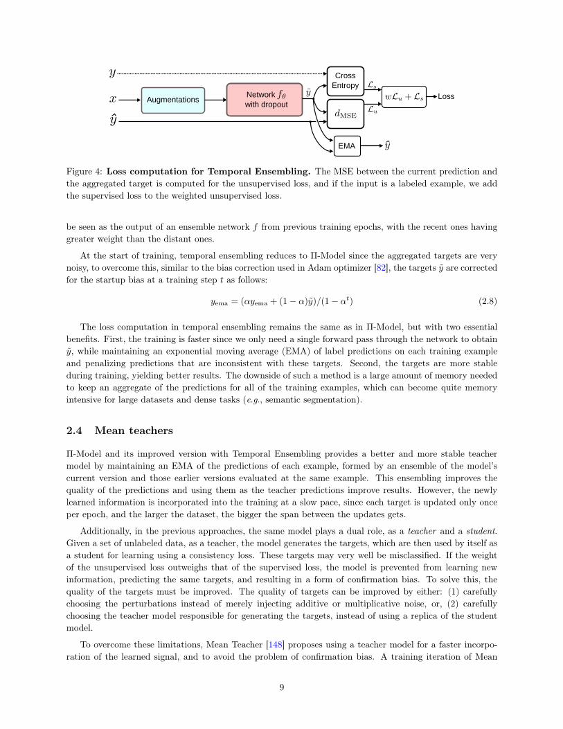
2.3 Temporal Ensembling

Π-Model can be divided into two stages, we first classify all of the training data without updating the weightsof the model, obtaining the predictions y, and in the second stage, we consider the predictions y as targets forthe unsupervised loss and enforce consistency of predictions by minimizing the distance between the currentoutputs y and the outputs of the first stage y under different dropouts and augmentations.

The problem with this approach is that the targets y are based on a single evaluation of the networkand can rapidly change. This instability in the targets can lead to an instability during training and reducesthe amount of training signal that can be extracted from the unlabeled examples. To solve this, Laine etal. [92] propose a second version of Π-Model called Temporal Ensembling, where the targets yema arethe aggregation of all the previous predictions. This way, during training, we only need a single forwardpass to get the current predictions y and the aggregated targets yema, speeding up the training time byapproximately 2×. The training process is illustrated in fig. 4.

For a target y, at each training iteration, the current output y is accumulated into the ensemble outputyema by an exponentially moving average update:

yema = αyema + (1− α)y (2.7)

where α is a momentum term that controls how far the ensemble reaches into training history. y can also

8

Networkwith dropout

Augmentations

CrossEntropy

Loss

EMA

Figure 4: Loss computation for Temporal Ensembling. The MSE between the current prediction andthe aggregated target is computed for the unsupervised loss, and if the input is a labeled example, we addthe supervised loss to the weighted unsupervised loss.

be seen as the output of an ensemble network f from previous training epochs, with the recent ones havinggreater weight than the distant ones.

At the start of training, temporal ensembling reduces to Π-Model since the aggregated targets are verynoisy, to overcome this, similar to the bias correction used in Adam optimizer [82], the targets y are correctedfor the startup bias at a training step t as follows:

yema = (αyema + (1− α)y)/(1− αt) (2.8)

The loss computation in temporal ensembling remains the same as in Π-Model, but with two essentialbenefits. First, the training is faster since we only need a single forward pass through the network to obtainy, while maintaining an exponential moving average (EMA) of label predictions on each training exampleand penalizing predictions that are inconsistent with these targets. Second, the targets are more stableduring training, yielding better results. The downside of such a method is a large amount of memory neededto keep an aggregate of the predictions for all of the training examples, which can become quite memoryintensive for large datasets and dense tasks (e.g., semantic segmentation).

2.4 Mean teachers

Π-Model and its improved version with Temporal Ensembling provides a better and more stable teachermodel by maintaining an EMA of the predictions of each example, formed by an ensemble of the model’scurrent version and those earlier versions evaluated at the same example. This ensembling improves thequality of the predictions and using them as the teacher predictions improve results. However, the newlylearned information is incorporated into the training at a slow pace, since each target is updated only onceper epoch, and the larger the dataset, the bigger the span between the updates gets.

Additionally, in the previous approaches, the same model plays a dual role, as a teacher and a student.Given a set of unlabeled data, as a teacher, the model generates the targets, which are then used by itself asa student for learning using a consistency loss. These targets may very well be misclassified. If the weightof the unsupervised loss outweighs that of the supervised loss, the model is prevented from learning newinformation, predicting the same targets, and resulting in a form of confirmation bias. To solve this, thequality of the targets must be improved. The quality of targets can be improved by either: (1) carefullychoosing the perturbations instead of merely injecting additive or multiplicative noise, or, (2) carefullychoosing the teacher model responsible for generating the targets, instead of using a replica of the studentmodel.

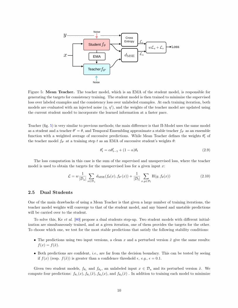
To overcome these limitations, Mean Teacher [148] proposes using a teacher model for a faster incorpo-ration of the learned signal, and to avoid the problem of confirmation bias. A training iteration of Mean

9

Student

CrossEntropy

Loss

Teacher

EMA

Noise

Noise

Figure 5: Mean Teacher. The teacher model, which is an EMA of the student model, is responsible forgenerating the targets for consistency training. The student model is then trained to minimize the supervisedloss over labeled examples and the consistency loss over unlabeled examples. At each training iteration, bothmodels are evaluated with an injected noise (η, η′), and the weights of the teacher model are updated usingthe current student model to incorporate the learned information at a faster pace.

Teacher (fig. 5) is very similar to previous methods; the main difference is that Π-Model uses the same modelas a student and a teacher θ′ = θ, and Temporal Ensembling approximate a stable teacher fθ′ as an ensemblefunction with a weighted average of successive predictions. While Mean Teacher defines the weights θ′t ofthe teacher model fθ′ at a training step t as an EMA of successive student’s weights θ:

θ′t = αθ′t−1 + (1− α)θt (2.9)

The loss computation in this case is the sum of the supervised and unsupervised loss, where the teachermodel is used to obtain the targets for the unsupervised loss for a given input x:

L = w1

|Du|∑x∈Du

dMSE(fθ(x), fθ′(x)) +1

|Dl|∑

x,y∈Dl

H(y, fθ(x)) (2.10)

2.5 Dual Students

One of the main drawbacks of using a Mean Teacher is that given a large number of training iterations, theteacher model weights will converge to that of the student model, and any biased and unstable predictionswill be carried over to the student.

To solve this, Ke et al. [80] propose a dual students step-up. Two student models with different initial-ization are simultaneously trained, and at a given iteration, one of them provides the targets for the other.To choose which one, we test for the most stable predictions that satisfy the following stability conditions:

• The predictions using two input versions, a clean x and a perturbed version x give the same results:f(x) = f(x).

• Both predictions are confident, i.e., are far from the decision boundary. This can be tested by seeingif f(x) (resp. f(x)) is greater than a confidence threshold ε, e.g., ε = 0.1.

Given two student models, fθ1 and fθ2 , an unlabeled input x ∈ Du and its perturbed version x. Wecompute four predictions: fθ1(x), fθ1(x), fθ2(x), and fθ2(x) . In addition to training each model to minimize

10

both the supervised and unsupervised losses:

L = Ls + λ1Lu =1

|Dl|∑

x,y∈Dl

H(y, fθi(x)) + λ11

|Du|∑x∈Du

dMSE(fθi(x), fθi(x)) (2.11)

we also force one of the students to have similar predictions to its counterpart. To chose which one to updateits weights, we check for both models’ stability constraint; if the predictions one of the models is unstable, weupdate its weights. If both are stable, we update the model with the largest variation E i = ‖fi(x)− fi(x)‖2,i.e., the least stable. In this case, the least stable model is trained with an additional loss:

λ2∑x∈Du

dMSE(fθi(x), fθj (x)) (2.12)

where λ1 and λ2 are hyperparameters specifying the contribution of each loss term.

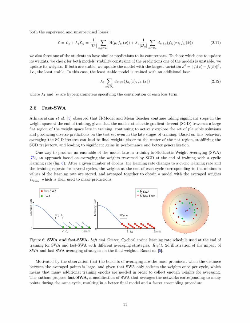
2.6 Fast-SWA

Athiwaratkun et al. [5] observed that Π-Model and Mean Teacher continue taking significant steps in theweight space at the end of training, given that the models stochastic gradient descent (SGD) traverses a largeflat region of the weight space late in training, continuing to actively explore the set of plausible solutionsand producing diverse predictions on the test set even in the late stages of training. Based on this behavior,averaging the SGD iterates can lead to final weights closer to the center of the flat region, stabilizing theSGD trajectory, and leading to significant gains in performance and better generalization.

One way to produce an ensemble of the model late in training is Stochastic Weight Averaging (SWA)[75], an approach based on averaging the weights traversed by SGD at the end of training with a cycliclearning rate (fig. 6). After a given number of epochs, the learning rate changes to a cyclic learning rate andthe training repeats for several cycles, the weights at the end of each cycle corresponding to the minimumvalues of the learning rate are stored, and averaged together to obtain a model with the averaged weightsfθSWA , which is then used to make predictions.

`0` Epoch

LearningRate

0

`0` Epoch

LearningRate

0

1Cycle1Cycle

SWA

fast-SWA

fast-SWA

SWA

Figure 6: SWA and fast-SWA. Left and Center. Cyclical cosine learning rate schedule used at the end oftraining for SWA and fast-SWA with different averaging strategies. Right. 2d illustration of the impact ofSWA and fast-SWA averaging strategies on the final weights. Based on [5].

Motivated by the observation that the benefits of averaging are the most prominent when the distancebetween the averaged points is large, and given that SWA only collects the weights once per cycle, whichmeans that many additional training epochs are needed in order to collect enough weights for averaging.The authors propose fast-SWA, a modification of SWA that averages the networks corresponding to manypoints during the same cycle, resulting in a better final model and a faster ensembling procedure.

11

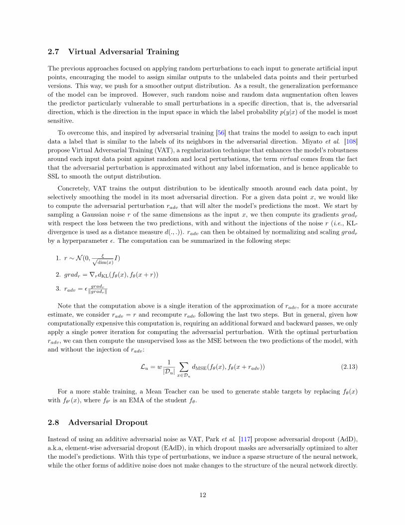
2.7 Virtual Adversarial Training

The previous approaches focused on applying random perturbations to each input to generate artificial inputpoints, encouraging the model to assign similar outputs to the unlabeled data points and their perturbedversions. This way, we push for a smoother output distribution. As a result, the generalization performanceof the model can be improved. However, such random noise and random data augmentation often leavesthe predictor particularly vulnerable to small perturbations in a specific direction, that is, the adversarialdirection, which is the direction in the input space in which the label probability p(y|x) of the model is mostsensitive.

To overcome this, and inspired by adversarial training [56] that trains the model to assign to each inputdata a label that is similar to the labels of its neighbors in the adversarial direction. Miyato et al. [108]propose Virtual Adversarial Training (VAT), a regularization technique that enhances the model’s robustnessaround each input data point against random and local perturbations, the term virtual comes from the factthat the adversarial perturbation is approximated without any label information, and is hence applicable toSSL to smooth the output distribution.

Concretely, VAT trains the output distribution to be identically smooth around each data point, byselectively smoothing the model in its most adversarial direction. For a given data point x, we would liketo compute the adversarial perturbation radv that will alter the model’s predictions the most. We start bysampling a Gaussian noise r of the same dimensions as the input x, we then compute its gradients gradrwith respect the loss between the two predictions, with and without the injections of the noise r (i.e., KL-divergence is used as a distance measure d(., .)). radv can then be obtained by normalizing and scaling gradrby a hyperparameter ε. The computation can be summarized in the following steps:

1. r ∼ N (0, ξ√dim(x)

I)

2. gradr = ∇rdKL(fθ(x), fθ(x+ r))

3. radv = ε gradr‖gradr‖

Note that the computation above is a single iteration of the approximation of radv, for a more accurateestimate, we consider radv = r and recompute radv following the last two steps. But in general, given howcomputationally expensive this computation is, requiring an additional forward and backward passes, we onlyapply a single power iteration for computing the adversarial perturbation. With the optimal perturbationradv, we can then compute the unsupervised loss as the MSE between the two predictions of the model, withand without the injection of radv:

Lu = w1

|Du|∑x∈Du

dMSE(fθ(x), fθ(x+ radv)) (2.13)

For a more stable training, a Mean Teacher can be used to generate stable targets by replacing fθ(x)

with fθ′(x), where fθ′ is an EMA of the student fθ.

2.8 Adversarial Dropout

Instead of using an additive adversarial noise as VAT, Park et al. [117] propose adversarial dropout (AdD),a.k.a, element-wise adversarial dropout (EAdD), in which dropout masks are adversarially optimized to alterthe model’s predictions. With this type of perturbations, we induce a sparse structure of the neural network,while the other forms of additive noise does not make changes to the structure of the neural network directly.

12

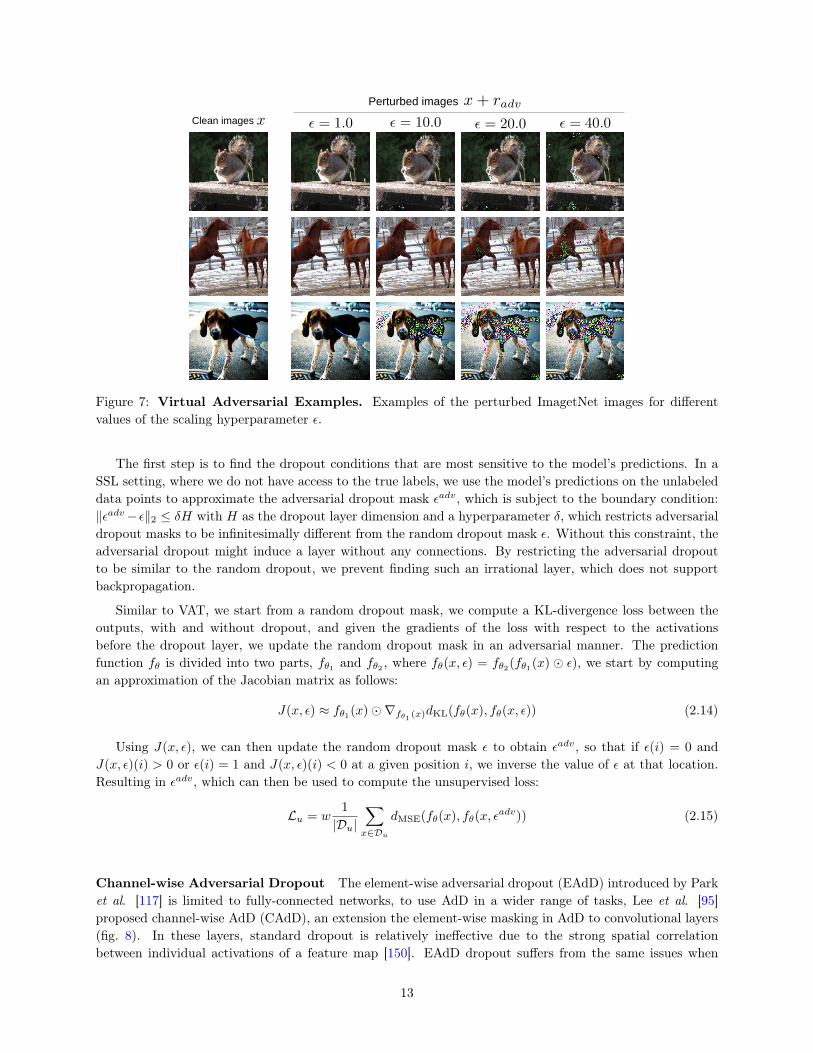
Perturbed images

Clean images

Figure 7: Virtual Adversarial Examples. Examples of the perturbed ImagetNet images for differentvalues of the scaling hyperparameter ε.

The first step is to find the dropout conditions that are most sensitive to the model’s predictions. In aSSL setting, where we do not have access to the true labels, we use the model’s predictions on the unlabeleddata points to approximate the adversarial dropout mask εadv, which is subject to the boundary condition:‖εadv− ε‖2 ≤ δH with H as the dropout layer dimension and a hyperparameter δ, which restricts adversarialdropout masks to be infinitesimally different from the random dropout mask ε. Without this constraint, theadversarial dropout might induce a layer without any connections. By restricting the adversarial dropoutto be similar to the random dropout, we prevent finding such an irrational layer, which does not supportbackpropagation.

Similar to VAT, we start from a random dropout mask, we compute a KL-divergence loss between theoutputs, with and without dropout, and given the gradients of the loss with respect to the activationsbefore the dropout layer, we update the random dropout mask in an adversarial manner. The predictionfunction fθ is divided into two parts, fθ1 and fθ2 , where fθ(x, ε) = fθ2(fθ1(x) � ε), we start by computingan approximation of the Jacobian matrix as follows:

J(x, ε) ≈ fθ1(x)�∇fθ1 (x)dKL(fθ(x), fθ(x, ε)) (2.14)

Using J(x, ε), we can then update the random dropout mask ε to obtain εadv, so that if ε(i) = 0 andJ(x, ε)(i) > 0 or ε(i) = 1 and J(x, ε)(i) < 0 at a given position i, we inverse the value of ε at that location.Resulting in εadv, which can then be used to compute the unsupervised loss:

Lu = w1

|Du|∑x∈Du

dMSE(fθ(x), fθ(x, εadv)) (2.15)

Channel-wise Adversarial Dropout The element-wise adversarial dropout (EAdD) introduced by Parket al. [117] is limited to fully-connected networks, to use AdD in a wider range of tasks, Lee et al. [95]proposed channel-wise AdD (CAdD), an extension the element-wise masking in AdD to convolutional layers(fig. 8). In these layers, standard dropout is relatively ineffective due to the strong spatial correlationbetween individual activations of a feature map [150]. EAdD dropout suffers from the same issues when

13

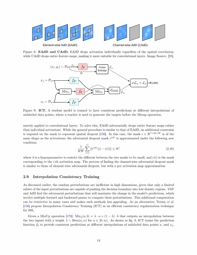
Element-wise AdD (EAdD) Channel-wise AdD (CAdD)

Figure 8: EAdD and CAdD. EAdD drops activation individually regardless of the spatial correlation,while CAdD drops entire feature maps, making it more suitable for convolutional layers. Image Source: [95].

CrossEntropy

Loss

Figure 9: ICT. A student model is trained to have consistent predictions at different interpolations ofunlabeled data points, where a teacher is used to generate the targets before the Mixup operation.

naively applied to convolutional layers. To solve this, EAdD adversarially drops entire feature maps ratherthan individual activations. While the general procedure is similar to that of EAdD, an additional constraintis imposed on the mask to represent spatial dropout [150]. In this case, the mask ε ∈ RC×H×W is of thesame shape as the activations; the adversarial dropout mask εadv is approximated under the following newcondition:

1

HW

C∑i=1

‖εadv(i)− ε(i)‖ ≤ δC (2.16)

where δ is a hyperparameter to restrict the different between the two masks to be small, and ε(i) is the maskcorresponding to the i-th activation map. The process of finding the channel-wise adversarial dropout maskis similar to those of element-wise adversarial dropout, but with a per activation map approximation.

2.9 Interpolation Consistency Training

As discussed earlier, the random perturbations are inefficient in high dimensions, given that only a limitedsubset of the input perturbations are capable of pushing the decision boundary into low-density regions. VATand AdD find the adversarial perturbations that will maximize the change in the model’s predictions, whichinvolve multiple forward and backward passes to compute these perturbations. This additional computationcan be restrictive in many cases and makes such methods less appealing. As an alternative, Verma et al.[156] propose Interpolation Consistency Training (ICT) as an efficient consistency regularization techniquefor SSL.

Given a MixUp operation [178]: Mixλ(a, b) = λ · a + (1 − λ) · b that outputs an interpolation betweenthe two inputs with a weight λ ∼ Beta(α, α) for α ∈ [0,∞]. As shown in fig. 9, ICT trains the predictionfunction fθ to provide consistent predictions at different interpolations of unlabeled data points xi and xj ,

14

where the targets are generated using a teacher model fθ′ which is an EMA of fθ:

fθ(Mixλ(xi, xj)) ≈ Mixλ(fθ′(xi), fθ′(xj)) (2.17)

The unsupervised objective is to have similar values between the student model’s prediction given amixed input of two unlabeled data points, and the mixed outputs of the teacher model.

Lu = w1

|Du|∑

xi,xj∈Du

dMSE(fθ(Mixλ(xi, xj)),Mixλ(fθ′(xi), fθ′(xj)) (2.18)

The benefit of ICT compared to random perturbations can be analyzed by considering the mixup oper-ation as a perturbation applied to a given unlabeled example: xi + δ = Mixλ(xi, xj), for a large number ofclasses and with a similar distribution of examples per class, it is likely that the pair of points (xi, xj) lie indifferent clusters and belong to different classes. If one of these two data points lies in a low-density region,applying an interpolation toward xj points to a low-density region, which is a good direction to move thedecision boundary toward.

2.10 Unsupervised Data Augmentation

Unsupervised Data Augmentation [169] uses advanced data augmentation methods, such as AutoAugment[29], RandAugment [30] and Back Translation [43, 139], as perturbations for consistency training based SSL.Similar to supervised learning, advanced data augmentation methods can also provide extra advantages oversimple augmentations and random noise injection in consistency training, given that; (1) it generates realisticaugmented examples, making it safe to encourage the consistency between predictions on the original andaugmented examples, (2) it can generate a diverse set of examples improving the sample efficiency, and (3)it is capable of providing the missing inductive biases for different tasks.

Motivated by these points, Xie et al. [169] propose to apply the following augmentations to generatetransformed versions of the unlabeled inputs:

• RandAugment for Image Classification. Consists of uniformly sampling from the same set ofpossible transformations in Python Imaging Library (PIL), without requiring any labeled data tosearch for a good augmentation strategy.

• Back-translation for Text Classification. Consists of translating an existing example in languageA into another language B, and then translating it back into A to obtain an augmented example.

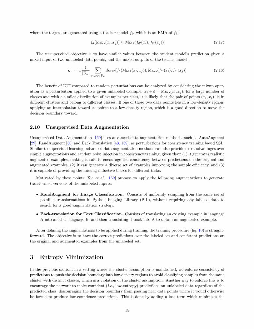
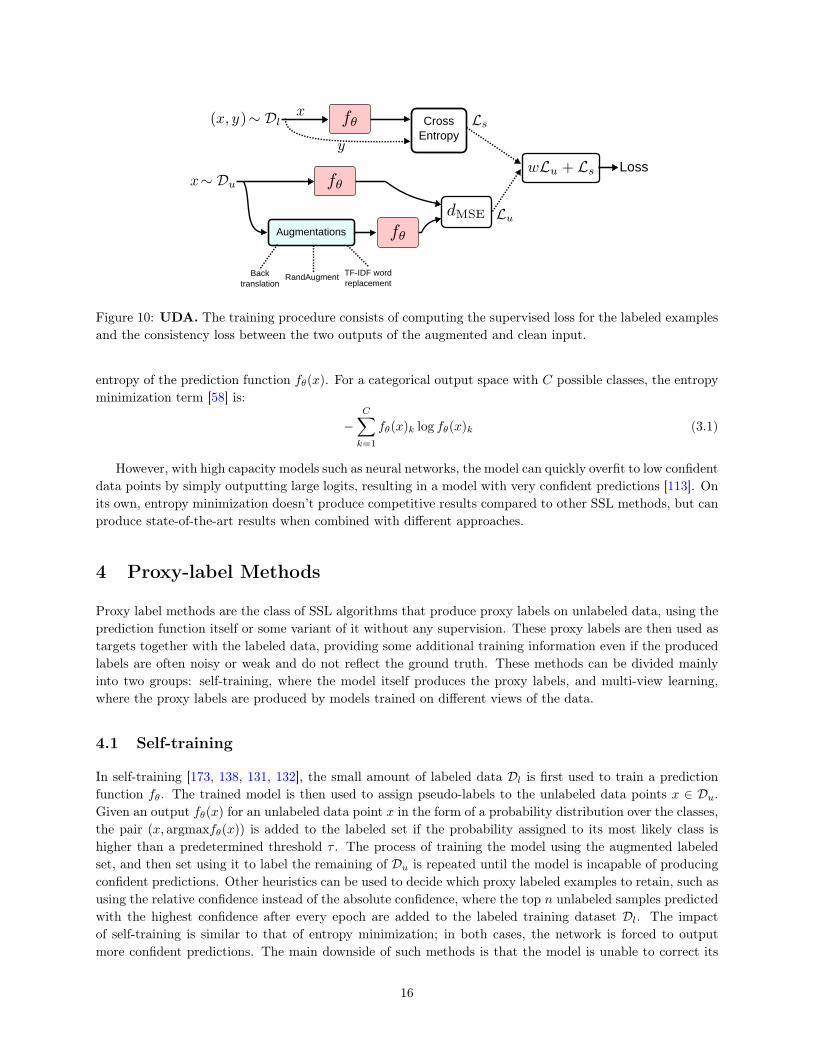
After defining the augmentations to be applied during training, the training procedure (fig. 10) is straight-forward. The objective is to have the correct predictions over the labeled set and consistent predictions onthe original and augmented examples from the unlabeled set.

3 Entropy Minimization

In the previous section, in a setting where the cluster assumption is maintained, we enforce consistency ofpredictions to push the decision boundary into low-density regions to avoid classifying samples from the samecluster with distinct classes, which is a violation of the cluster assumption. Another way to enforce this is toencourage the network to make confident (i.e., low-entropy) predictions on unlabeled data regardless of thepredicted class, discouraging the decision boundary from passing near data points where it would otherwisebe forced to produce low-confidence predictions. This is done by adding a loss term which minimizes the

15

CrossEntropy

Loss

Augmentations

Backtranslation

RandAugment TF-IDF wordreplacement

Figure 10: UDA. The training procedure consists of computing the supervised loss for the labeled examplesand the consistency loss between the two outputs of the augmented and clean input.

entropy of the prediction function fθ(x). For a categorical output space with C possible classes, the entropyminimization term [58] is:

−C∑k=1

fθ(x)k log fθ(x)k (3.1)

However, with high capacity models such as neural networks, the model can quickly overfit to low confidentdata points by simply outputting large logits, resulting in a model with very confident predictions [113]. Onits own, entropy minimization doesn’t produce competitive results compared to other SSL methods, but canproduce state-of-the-art results when combined with different approaches.

4 Proxy-label Methods

Proxy label methods are the class of SSL algorithms that produce proxy labels on unlabeled data, using theprediction function itself or some variant of it without any supervision. These proxy labels are then used astargets together with the labeled data, providing some additional training information even if the producedlabels are often noisy or weak and do not reflect the ground truth. These methods can be divided mainlyinto two groups: self-training, where the model itself produces the proxy labels, and multi-view learning,where the proxy labels are produced by models trained on different views of the data.

4.1 Self-training

In self-training [173, 138, 131, 132], the small amount of labeled data Dl is first used to train a predictionfunction fθ. The trained model is then used to assign pseudo-labels to the unlabeled data points x ∈ Du.Given an output fθ(x) for an unlabeled data point x in the form of a probability distribution over the classes,the pair (x, argmaxfθ(x)) is added to the labeled set if the probability assigned to its most likely class ishigher than a predetermined threshold τ . The process of training the model using the augmented labeledset, and then set using it to label the remaining of Du is repeated until the model is incapable of producingconfident predictions. Other heuristics can be used to decide which proxy labeled examples to retain, such asusing the relative confidence instead of the absolute confidence, where the top n unlabeled samples predictedwith the highest confidence after every epoch are added to the labeled training dataset Dl. The impactof self-training is similar to that of entropy minimization; in both cases, the network is forced to outputmore confident predictions. The main downside of such methods is that the model is unable to correct its

16

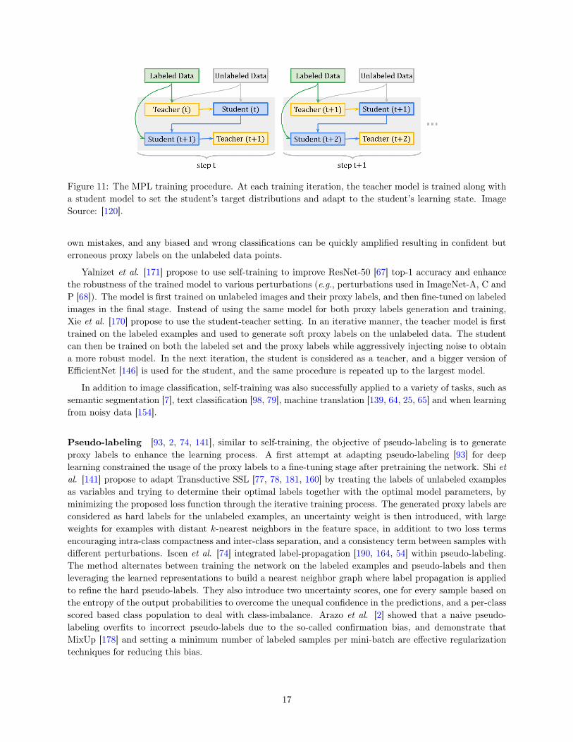
Figure 11: The MPL training procedure. At each training iteration, the teacher model is trained along witha student model to set the student’s target distributions and adapt to the student’s learning state. ImageSource: [120].

own mistakes, and any biased and wrong classifications can be quickly amplified resulting in confident buterroneous proxy labels on the unlabeled data points.

Yalnizet et al. [171] propose to use self-training to improve ResNet-50 [67] top-1 accuracy and enhancethe robustness of the trained model to various perturbations (e.g., perturbations used in ImageNet-A, C andP [68]). The model is first trained on unlabeled images and their proxy labels, and then fine-tuned on labeledimages in the final stage. Instead of using the same model for both proxy labels generation and training,Xie et al. [170] propose to use the student-teacher setting. In an iterative manner, the teacher model is firsttrained on the labeled examples and used to generate soft proxy labels on the unlabeled data. The studentcan then be trained on both the labeled set and the proxy labels while aggressively injecting noise to obtaina more robust model. In the next iteration, the student is considered as a teacher, and a bigger version ofEfficientNet [146] is used for the student, and the same procedure is repeated up to the largest model.

In addition to image classification, self-training was also successfully applied to a variety of tasks, such assemantic segmentation [7], text classification [98, 79], machine translation [139, 64, 25, 65] and when learningfrom noisy data [154].

Pseudo-labeling [93, 2, 74, 141], similar to self-training, the objective of pseudo-labeling is to generateproxy labels to enhance the learning process. A first attempt at adapting pseudo-labeling [93] for deeplearning constrained the usage of the proxy labels to a fine-tuning stage after pretraining the network. Shi etal. [141] propose to adapt Transductive SSL [77, 78, 181, 160] by treating the labels of unlabeled examplesas variables and trying to determine their optimal labels together with the optimal model parameters, byminimizing the proposed loss function through the iterative training process. The generated proxy labels areconsidered as hard labels for the unlabeled examples, an uncertainty weight is then introduced, with largeweights for examples with distant k-nearest neighbors in the feature space, in additiont to two loss termsencouraging intra-class compactness and inter-class separation, and a consistency term between samples withdifferent perturbations. Iscen et al. [74] integrated label-propagation [190, 164, 54] within pseudo-labeling.The method alternates between training the network on the labeled examples and pseudo-labels and thenleveraging the learned representations to build a nearest neighbor graph where label propagation is appliedto refine the hard pseudo-labels. They also introduce two uncertainty scores, one for every sample based onthe entropy of the output probabilities to overcome the unequal confidence in the predictions, and a per-classscored based class population to deal with class-imbalance. Arazo et al. [2] showed that a naive pseudo-labeling overfits to incorrect pseudo-labels due to the so-called confirmation bias, and demonstrate thatMixUp [178] and setting a minimum number of labeled samples per mini-batch are effective regularizationtechniques for reducing this bias.

17

Meta Pseudo Labels Given how important the heuristics used to select which the proxy labels to addto the training set, where a proper method could lead to a sizable gain. Pham et al. [120] propose to usethe student-teacher setting, where the teacher model is responsible for producing the proxy labels basedon an efficient meta-learning algorithm called Meta Pseudo Labels (MPL), which encourages the teacher toadjust the target distributions of training examples in a manner that improves the learning of the studentmodel. The teacher is updated by policy gradients computed by evaluating the student model on a held-outvalidation set.

A given training step of MPL consists of two phases (fig. 11):

• Phase 1: The Student learns from the Teacher. In this phase, given a single input example x ∈ Dl,the teacher fθ′ produces a target class-distribution to train the student fθ, where the pair (x, fθ′(x))

is shown to the student to update its parameters by back-propagating from the cross-entropy loss.

• Phase 2: The Teacher learns from the Student’s Validation Loss. After the student updates itsparameters in first step, its new parameter θ(t+ 1) are evaluated on an example (xval, yval) from theheld-out validation dataset using the cross-entropy loss. Since the validation loss depends on θ′ viathe first step, this validation cross-entropy loss is also a function of the teacher’s weights θ′. Thisdependency allows us to compute the gradients of the validation loss with respect to the teacher’sweights, and then update θ′ to minimize the validation loss using policy gradients.

While the student’s performance allows the teacher to adjust and adapt to the student’s learning state,this signal alone is not sufficient to train the teacher since when the teacher has observed enough evidenceto produce meaningful target distributions to teach the student, the student might have already entered abad region of parameters. To overcome this, the teacher is also trained using the pair of labeled data pointsfrom the held-out validation set.

4.2 Multi-view training

Multi-view training (MVL) [89, 182] utilizes multi-view data that are very common in real-world applications,where different views can be collected by different measuring methods (e.g., color information and textureinformation for images) or by creating limited views of the original data. In such a setting, MVL aims tolearn a distinct prediction function fθi to model a given view vi(x) of a data point x, and jointly optimize allthe functions to improve the generalization performance. Ideally, the possible views complement each otherso that the produced models can collaborate in improving each other’s performance.

4.2.1 Co-training

Co-training [16] requires that each data point x can be represented using two conditionally independentviews v1(x) and v2(x), and that each view is sufficient to train a good model. After training two predictionfunctions fθ1 and fθ2 on a specific view on the labeled set Dl. We start the proxy labeling procedure. Ateach iteration, an unlabeled data point is added to the training set of the model fθi if the other model fθjoutputs a confident prediction with a probability higher than a threshold τ . This way, one of the modelsprovides newly labeled examples where the other model is uncertain. Co-training has been combined withdeep learning for some applications, such as object recognition [24] by utilizing RGB-D data, with RGB anddepth as the two views used to train the two models, or for combining multi-modal data [3] (i.e., imageand text) by training each model on a given modality and use it to provide pseudo-labels for other models.However, in many cases, the data have only one view rather than two, in this instance, different learningalgorithms or different parameter configurations to learn two different classifiers can be employed. The twoviews v1(x) and v2(x) can also be generated by injecting noise or by applying different augmentations, for

18

example, Qiao et al. [121] used adversarial perturbations to produce new views for deep co-training for imageclassification, where the models are encouraged to have the same predictions on Dl but make different errorswhen they are exposed to adversarial attacks.

Democratic Co-training [187]. An extension of Co-training, consists of replacing the different views ofthe input data with a number of models with different architectures and learning algorithms, which are firsttrained on the labeled examples. The trained models are then used to label a given example x if a majorityof models confidently agree on its label.

4.2.2 Tri-Training

Tri-training [189] tries to overcome the lack of data with multiple views and reduce the bias of the predictionson unlabeled data produced with self-training by utilizing the agreement of three independently trainedmodels instead of a single model. First, the labeled data Dl is used to train three prediction functions: fθ1 ,fθ2 and fθ3 . An unlabeled data point x ∈ Du is then added to the supervised training set of the function fθiif the other two models agree on its predicted label. The training stops if no data points are being addedto any of the models’ training sets. Tri-training requires neither the existence of multiple views nor uniquelearning algorithms, making it more generally applicable. Using Tri-training with neural networks can bevery expensive, requiring predictions for each one of the three models on all the unlabeled data. Ruder etal. [133] propose to sample a limited number of unlabeled data points at each training epoch, the candidatepool size is increased as the training progresses and the models become more accurate.

Multi-task tri-training [133] can also be used to reduce the time and sample complexity, where all threemodels share the same feature-extractor with model-specific classification layers. This way, the models aretrained jointly with an additional orthogonality constraint on two of the three classification layers to beadded to loss term, to avoid learning similar models and falling back to the standard case of self-training.Tri-Net [39] also falls in this category, with a shared module for joint learning and three output modules fortri-training, in addition to utilizing output smearing [17] to initialize these modules. After the proxy labelingiteration, a fine-tuning stage is conducted on the labeled data to augment diversity and eliminate unstableand suspicious pseudo-labeled data.

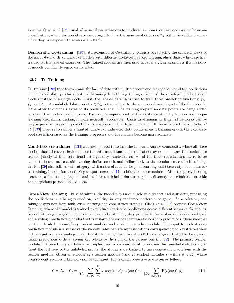
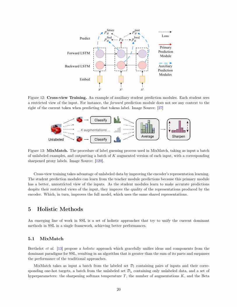
Cross-View Training In self-training, the model plays a dual role of a teacher and a student, producingthe predictions it is being trained on, resulting in very moderate performance gains. As a solution, andtaking inspiration from multi-view learning and consistency training, Clark et al. [27] propose Cross-ViewTraining, where the model is trained to produce consistent predictions across different views of the inputs.Instead of using a single model as a teacher and a student, they propose to use a shared encoder, and thenadd auxiliary prediction modules that transform the encoder representations into predictions, these modulesare then divided into auxiliary student modules and a primary teacher module. The input to each studentprediction module is a subset of the model’s intermediate representations corresponding to a restricted viewof the input, such as feeding one of the student only the forward LSTM from a given Bi-LSTM layer, so itmakes predictions without seeing any tokens to the right of the current one (fig. 12). The primary teachermodule in trained only on labeled examples, and is responsible of generating the pseudo-labels taking asinput the full view of the unlabeled inputs, the students are trained to have consistent predictions with theteacher module. Given an encoder e, a teacher module t and K student modules si with i ∈ [0,K], whereeach student receives a limited view of the input, the training objective is written as follows:

L = Lu + Ls =1

|Du|∑x∈Du

K∑i=1

dMSE(t(e(x)), si(e(x))) +1

|Dl|∑

x,y∈Dl

H(t(e(x)), y) (4.1)

19

LSTM LSTM

ŷfuture  ŷfwd  ŷ   ŷbwd  ŷpast 

Backward LSTM

Forward LSTM

Predict

LSTM LSTM

LSTM

LSTM LSTM

AuxiliaryPredictionModules

PrimaryPredictionModule

x1 x2 x3

Embed

Backward LSTM

Forward LSTM

pθPredict pfwdθ

pfutureθ

pbwdθ

ppastθ

AuxiliaryPredictionModules

PrimaryPredictionModule

Loss

Figure 12: Cross-view Training. An example of auxiliary student prediction modules. Each student seesa restricted view of the input. For instance, the forward prediction module does not see any context to theright of the current token when predicting that tokens label. Image Source: [27]

Figure 13: MixMatch. The procedure of label guessing process used in MixMatch, taking as input a batchof unlabeled examples, and outputting a batch of K augmented version of each input, with a correspondingsharpened proxy labels. Image Source: [120].

Cross-view training takes advantage of unlabeled data by improving the encoder’s representation learning.The student prediction modules can learn from the teacher module predictions because this primary modulehas a better, unrestricted view of the inputs. As the student modules learn to make accurate predictionsdespite their restricted views of the input, they improve the quality of the representations produced by theencoder. Which, in turn, improves the full model, which uses the same shared representations.

5 Holistic Methods

An emerging line of work in SSL is a set of holistic approaches that try to unify the current dominantmethods in SSL in a single framework, achieving better performances.

5.1 MixMatch

Berthelot et al. [13] propose a holistic approach which gracefully unifies ideas and components from thedominant paradigms for SSL, resulting in an algorithm that is greater than the sum of its parts and surpassesthe performance of the traditional approaches.

MixMatch takes as input a batch from the labeled set Dl containing pairs of inputs and their corre-sponding one-hot targets, a batch from the unlabeled set Du containing only unlabeled data, and a set ofhyperparameters: the sharpening softmax temperature T , the number of augmentations K, and the Beta

20

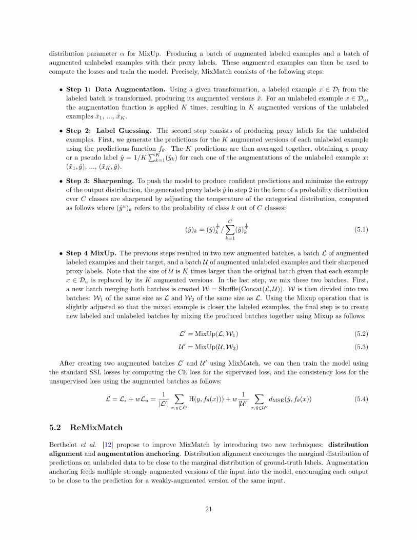
distribution parameter α for MixUp. Producing a batch of augmented labeled examples and a batch ofaugmented unlabeled examples with their proxy labels. These augmented examples can then be used tocompute the losses and train the model. Precisely, MixMatch consists of the following steps:

• Step 1: Data Augmentation. Using a given transformation, a labeled example x ∈ Dl from thelabeled batch is transformed, producing its augmented versions x. For an unlabeled example x ∈ Du,the augmentation function is applied K times, resulting in K augmented versions of the unlabeledexamples x1, ..., xK .

• Step 2: Label Guessing. The second step consists of producing proxy labels for the unlabeledexamples. First, we generate the predictions for the K augmented versions of each unlabeled exampleusing the predictions function fθ. The K predictions are then averaged together, obtaining a proxyor a pseudo label y = 1/K

∑Kk=1(yk) for each one of the augmentations of the unlabeled example x:

(x1, y), ..., (xK , y).

• Step 3: Sharpening. To push the model to produce confident predictions and minimize the entropyof the output distribution, the generated proxy labels y in step 2 in the form of a probability distributionover C classes are sharpened by adjusting the temperature of the categorical distribution, computedas follows where (yu)k refers to the probability of class k out of C classes:

(y)k = (y)1T

k /

C∑k=1

(y)1T

k (5.1)

• Step 4 MixUp. The previous steps resulted in two new augmented batches, a batch L of augmentedlabeled examples and their target, and a batch U of augmented unlabeled examples and their sharpenedproxy labels. Note that the size of U is K times larger than the original batch given that each examplex ∈ Du is replaced by its K augmented versions. In the last step, we mix these two batches. First,a new batch merging both batches is created W = Shuffle(Concat(L,U)). W is then divided into twobatches: W1 of the same size as L and W2 of the same size as L. Using the Mixup operation that isslightly adjusted so that the mixed example is closer the labeled examples, the final step is to createnew labeled and unlabeled batches by mixing the produced batches together using Mixup as follows:

L′ = MixUp(L,W1) (5.2)

U ′ = MixUp(U ,W2) (5.3)

After creating two augmented batches L′ and U ′ using MixMatch, we can then train the model usingthe standard SSL losses by computing the CE loss for the supervised loss, and the consistency loss for theunsupervised loss using the augmented batches as follows:

L = Ls + wLu =1

|L′|∑x,y∈L′

H(y, fθ(x))) + w1

|U ′|∑

x,y∈U ′

dMSE(y, fθ(x)) (5.4)

5.2 ReMixMatch

Berthelot et al. [12] propose to improve MixMatch by introducing two new techniques: distributionalignment and augmentation anchoring. Distribution alignment encourages the marginal distribution ofpredictions on unlabeled data to be close to the marginal distribution of ground-truth labels. Augmentationanchoring feeds multiple strongly augmented versions of the input into the model, encouraging each outputto be close to the prediction for a weakly-augmented version of the same input.

21

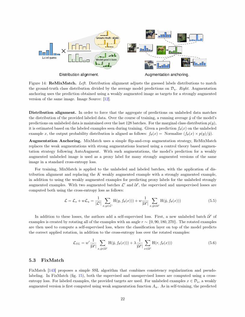
Figure 14: ReMixMatch. Left. Distribution alignment adjusts the guessed labels distributions to matchthe ground-truth class distribution divided by the average model predictions on Du. Right. Augmentationanchoring uses the prediction obtained using a weakly augmented image as targets for a strongly augmentedversion of the same image. Image Source: [12].

Distribution alignment. In order to force that the aggregate of predictions on unlabeled data matchesthe distribution of the provided labeled data. Over the course of training, a running average y of the model’spredictions on unlabeled data is maintained over the last 128 batches. For the marginal class distribution p(y),it is estimated based on the labeled examples seen during training. Given a prediction fθ(x) on the unlabeledexample x, the output probability distribution is aligned as follows: fθ(x) = Normalize (fθ(x)× p(y)/y).

Augmentation Anchoring. MixMatch uses a simple flip-and-crop augmentation strategy, ReMixMatchreplaces the weak augmentations with strong augmentations learned using a control theory based augmen-tation strategy following AutoAugment. With such augmentations, the model’s prediction for a weaklyaugmented unlabeled image is used as a proxy label for many strongly augmented versions of the sameimage in a standard cross-entropy loss.

For training, MixMatch is applied to the unlabeled and labeled batches, with the application of dis-tribution alignment and replacing the K weakly augmented example with a strongly augmented example,in addition to using the weakly augmented examples for predicting proxy labels for the unlabeled stronglyaugmented examples. With two augmented batches L′ and U ′, the supervised and unsupervised losses arecomputed both using the cross-entropy loss as follows:

L = Ls + wLu =1

|L′|∑x,y∈L′

H(y, fθ(x))) + w1

|U ′|∑

x,y∈U ′

H(y, fθ(x))) (5.5)

In addition to these losses, the authors add a self-supervised loss. First, a new unlabeled batch U ′ ofexamples is created by rotating all of the examples with an angle r ∼ {0, 90, 180, 270}. The rotated examplesare then used to compute a self-supervised loss, where the classification layer on top of the model predictsthe correct applied rotation, in addition to the cross-entropy loss over the rotated examples:

LSL = w′1

|U ′|

∑x,y∈U ′

H(y, fθ(x))) + λ1

|U ′|

∑x∈U ′

H(r, fθ(x))) (5.6)

5.3 FixMatch

FixMatch [143] proposes a simple SSL algorithm that combines consistency regularization and pseudo-labeling. In FixMatch (fig. 15), both the supervised and unsupervised losses are computed using a cross-entropy loss. For labeled examples, the provided targets are used. For unlabeled examples x ∈ Du, a weaklyaugmented version is first computed using weak augmentation function Aw. As in self-training, the predicted

22

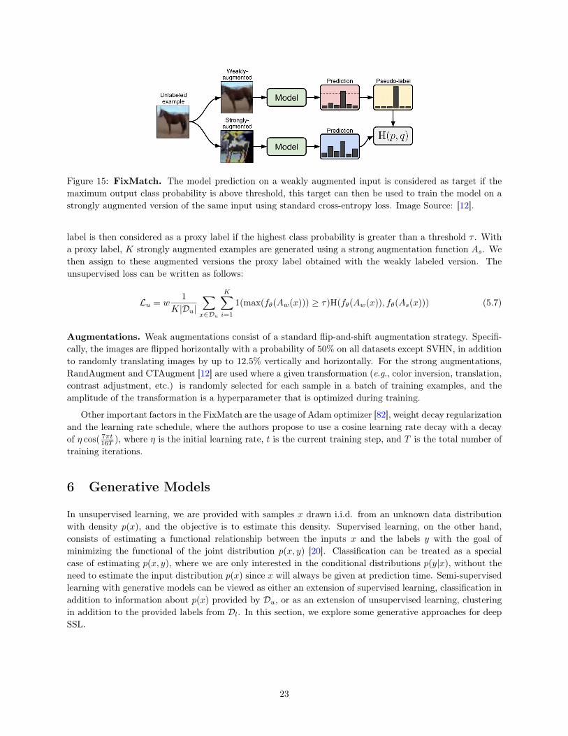
Figure 15: FixMatch. The model prediction on a weakly augmented input is considered as target if themaximum output class probability is above threshold, this target can then be used to train the model on astrongly augmented version of the same input using standard cross-entropy loss. Image Source: [12].

label is then considered as a proxy label if the highest class probability is greater than a threshold τ . Witha proxy label, K strongly augmented examples are generated using a strong augmentation function As. Wethen assign to these augmented versions the proxy label obtained with the weakly labeled version. Theunsupervised loss can be written as follows:

Lu = w1

K|Du|∑x∈Du

K∑i=1

1(max(fθ(Aw(x))) ≥ τ)H(fθ(Aw(x)), fθ(As(x))) (5.7)

Augmentations. Weak augmentations consist of a standard flip-and-shift augmentation strategy. Specifi-cally, the images are flipped horizontally with a probability of 50% on all datasets except SVHN, in additionto randomly translating images by up to 12.5% vertically and horizontally. For the strong augmentations,RandAugment and CTAugment [12] are used where a given transformation (e.g., color inversion, translation,contrast adjustment, etc.) is randomly selected for each sample in a batch of training examples, and theamplitude of the transformation is a hyperparameter that is optimized during training.

Other important factors in the FixMatch are the usage of Adam optimizer [82], weight decay regularizationand the learning rate schedule, where the authors propose to use a cosine learning rate decay with a decayof η cos( 7πt

16T ), where η is the initial learning rate, t is the current training step, and T is the total number oftraining iterations.

6 Generative Models

In unsupervised learning, we are provided with samples x drawn i.i.d. from an unknown data distributionwith density p(x), and the objective is to estimate this density. Supervised learning, on the other hand,consists of estimating a functional relationship between the inputs x and the labels y with the goal ofminimizing the functional of the joint distribution p(x, y) [20]. Classification can be treated as a specialcase of estimating p(x, y), where we are only interested in the conditional distributions p(y|x), without theneed to estimate the input distribution p(x) since x will always be given at prediction time. Semi-supervisedlearning with generative models can be viewed as either an extension of supervised learning, classification inaddition to information about p(x) provided by Du, or as an extension of unsupervised learning, clusteringin addition to the provided labels from Dl. In this section, we explore some generative approaches for deepSSL.

23

6.1 Variational Autoencoders for SSL

Variational Autoencoders (VAEs) [83, 36] have emerged as one of the most popular approaches to unsuper-vised learning of complicated distributions. A standard VAE is an autoencoder trained with a reconstructionobjective between the inputs and their reconstructed versions, in addition to a variational objective termthat attempts to learn a latent space that roughly follows a unit Gaussian distribution, this objective isimplemented as the KL-divergence between the latent space and the standard Gaussian. With an input x,the conditional distribution qφ(z|x) modeled by an encoder, the standard Gaussian distribution p(z) and thereconstructed input x generated using a decoder pθ(x|z). The parameters φ and θ are trained to minimizethe following objective:

L = dMSE(x, x) + dKL(qφ(z|x), p(z)) (6.1)

6.1.1 Variational Autoencoder

Kingma et al. [84] expanded the work on variational generative techniques [83, 128] for SSL, that exploitgenerative descriptions of the data to improve upon the classification performance that would be obtainedusing the labeled data alone.

Standard VAEs for SSL (M1 Model) The first model consists of an unsupervised pretraining stage,in which the VAE is trained using the labeled and unlabeled examples. Using a fully trained VAE, theobserved labeled data x ∈ Dl are transformed into the latent space defined by z, the standard supervisedtask can then be solved using (z, y) where y are the labels of x. With this approach, the classification canbe performed in a lower dimensional space since the dimensionality of the latent variables z is much lessthan that of the observations. These low dimensional embeddings are more easily separable since the latentspace is formed by independent Gaussian posteriors parameterized by an encoder, built by a sequence ofnon-linear transformations of the inputs.

Extending VAEs for SSL (M2 Model) In the M1 model, the labels of Dl were ignored when trainingthe VAE. With the second model, the labels are also used during training. If the class labels are not available,y is treated as a latent variable in addition to the latent variable z. The network in this case contains threecomponents, qφ(y|x) modeled by a classification network, qφ(z|y, x) modeled by an encoder, and pθ(x|y, z)modeled by a decoder, with parameters φ and θ. The training is similar to a standard VAE with the additionof the posterior on y and loss terms to train qφ(y|x) if the labels are available. The distribution qφ(y|x) canthen be used at test time to get the predictions on unseen data.

Stacked VAEs (M1+M2 Model) The two previous models can be concatenated to form a joint model.In this case, the model M1 is first trained to obtain the latent variables z1, the model M2 then uses thelatent variables z1 from model M1 as new representations of the data as opposed to raw values x. The finalmodel can be described as follows:

pθ(x, y, z1, z2) = p(y)p(z2)pθ(z1|y, z2)pθ(x|z1) (6.2)

6.1.2 Variational Auxiliary Autoencoder

Variational Auxiliary Autoencoder [102, 124] extends the variational distribution with auxiliary variables a:q(a, z|x) = q(z|a, x)q(a|x), such that the marginal distribution q(z|x) can fit more complicated posteriorsp(z|x) while improving the flexibility of inference. In order to have an unchanged generative model p(x|z),

24

Generator

Latent space

Discriminator

Real samples

Generatedsamples

"real"or

"fake"

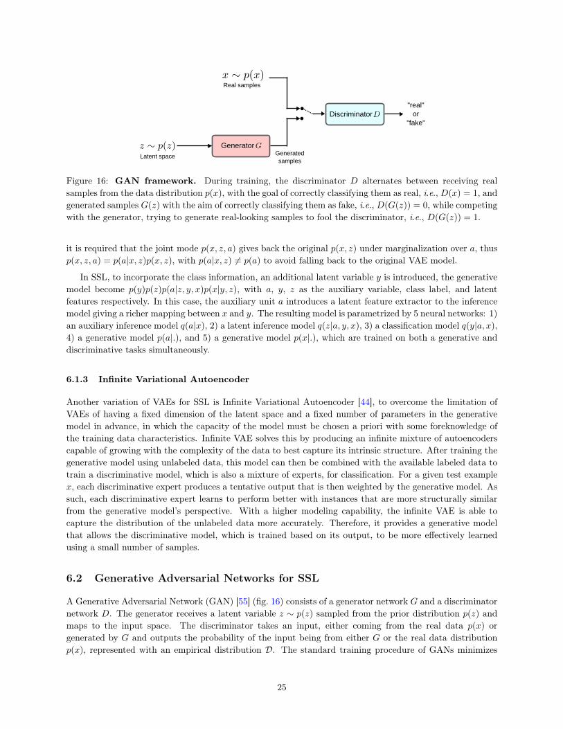
Figure 16: GAN framework. During training, the discriminator D alternates between receiving realsamples from the data distribution p(x), with the goal of correctly classifying them as real, i.e., D(x) = 1, andgenerated samples G(z) with the aim of correctly classifying them as fake, i.e., D(G(z)) = 0, while competingwith the generator, trying to generate real-looking samples to fool the discriminator, i.e., D(G(z)) = 1.

it is required that the joint mode p(x, z, a) gives back the original p(x, z) under marginalization over a, thusp(x, z, a) = p(a|x, z)p(x, z), with p(a|x, z) 6= p(a) to avoid falling back to the original VAE model.

In SSL, to incorporate the class information, an additional latent variable y is introduced, the generativemodel become p(y)p(z)p(a|z, y, x)p(x|y, z), with a, y, z as the auxiliary variable, class label, and latentfeatures respectively. In this case, the auxiliary unit a introduces a latent feature extractor to the inferencemodel giving a richer mapping between x and y. The resulting model is parametrized by 5 neural networks: 1)an auxiliary inference model q(a|x), 2) a latent inference model q(z|a, y, x), 3) a classification model q(y|a, x),4) a generative model p(a|.), and 5) a generative model p(x|.), which are trained on both a generative anddiscriminative tasks simultaneously.

6.1.3 Infinite Variational Autoencoder

Another variation of VAEs for SSL is Infinite Variational Autoencoder [44], to overcome the limitation ofVAEs of having a fixed dimension of the latent space and a fixed number of parameters in the generativemodel in advance, in which the capacity of the model must be chosen a priori with some foreknowledge ofthe training data characteristics. Infinite VAE solves this by producing an infinite mixture of autoencoderscapable of growing with the complexity of the data to best capture its intrinsic structure. After training thegenerative model using unlabeled data, this model can then be combined with the available labeled data totrain a discriminative model, which is also a mixture of experts, for classification. For a given test examplex, each discriminative expert produces a tentative output that is then weighted by the generative model. Assuch, each discriminative expert learns to perform better with instances that are more structurally similarfrom the generative model’s perspective. With a higher modeling capability, the infinite VAE is able tocapture the distribution of the unlabeled data more accurately. Therefore, it provides a generative modelthat allows the discriminative model, which is trained based on its output, to be more effectively learnedusing a small number of samples.

6.2 Generative Adversarial Networks for SSL

A Generative Adversarial Network (GAN) [55] (fig. 16) consists of a generator network G and a discriminatornetwork D. The generator receives a latent variable z ∼ p(z) sampled from the prior distribution p(z) andmaps to the input space. The discriminator takes an input, either coming from the real data p(x) orgenerated by G and outputs the probability of the input being from either G or the real data distributionp(x), represented with an empirical distribution D. The standard training procedure of GANs minimizes

25

two objectives by alternating between training the discriminator D and the generator G:

LD = maxD

Ex∼p(x)[logD(x)] + Ez∼p(z)[1− logD(G(z))]

LG = minG−Ez∼p(z)[logD(G(z))]

(6.3)

where p(z) is usually chosen as a standard normal distribution. Other formulations have been proposed toimprove and stabilize the training procedure, such as the hinge-loss version of the adversarial loss [99, 151]and Wassertein GAN (WGAN) [4]. Which are subsequently improved in several ways [176, 107, 177], such asusing spectral normalization [107] on both the generator and the discriminator, or consistency regularizationon the discriminator [177].

6.2.1 CatGAN

Categorical generative adversarial networks (CatGAN) [145] consist of combining both the generative andthe discriminative perspectives within the training procedure. The discriminator D in this case plays the roleof C classifiers and is trained to maximize the mutual information between the inputs x and the predictedlabels for a number of C unknown classes. To aid these classifiers in their task of discovering categories thatgeneralize well to unseen data, and avoid overfitting to spurious correlations in the data, the adversarialgenerative network comes into play and provides the examples the discriminator must become robust to.

The traditional two-player game in the GAN framework can be extended to CatGAN by having a dis-criminator that assign all examples to one the C classes instead of a probability of x belonging to p(x), whilestaying uncertain of the class assignments for the generated samples by G. After training such a classifier-generator pair where the discovered C classes coincide with the classification problem we are interested in,the classifier can then be used during inference being trained only on unlabeled data.

CatGAN objective dictates three requirements for the discriminator and two requirements that the gen-erator should fulfilled:• Discriminator requirements: should (1) be certain of class assignment for samples from p(x), (2) be

uncertain of assignment for generated samples, and (3) by assuming a uniform prior p(y) over classes,all classes must be distributed equally.

• Generator requirements: should (1) generate samples with highly certain class assignments, and (2)similar to the discriminator, equally distribute samples across all classes.

In order to have the output class distribution D(x) = p(y|x,D) to be highly peaked where D is certainabout the class assignment, the entropy H(D(x)) of the class distribution must be low. For the generatedsamples D(G(z)) = p(y|G(z), D), the predictions should be highly uncertain with a uniform class distribu-tion, in this case, the entropy H(D(G(z))) must be high. The first two requirements can then be enforced bysimply minimizing H(D(x)) and maximizing the H(D(G(z))). To meet the third requirement that all classesshould be used equally, the entropy of the marginal class distribution as measured empirically for both Dand G needs to be maximized:

HD = H

(1

N

N∑i=1

D(xi)

)

HG ≈ H

(1

M

M∑i=1

D(G(zi))

) (6.4)

Combining these requirements, CatGAN objective for the discriminator and the generator is:

LD = maxD−Ex∼p(x)[H(D(x))] + Ez∼p(z)[H(D(G(z)))] + HD

LG = minG

Ez∼p(z)[H(D(G(z)))]−HG

(6.5)

26

In SSL, if the input x comes from the labeled set Dl with a label y in the form of a one-hot vector, thediscriminator D is trained with a cross-entropy loss in addition to LD:

LD + λE(x,y)∼p(x)l [−y logG(x)] (6.6)

where λ is a cost weighting term.

6.2.2 DCGAN

Another way of using GANs for SSL is to leverage the unlabeled examples to learn good and transferableintermediate representations, which can then be used on a variety of supervised learning tasks such as imageclassification based on a small labeled set Dl. Radford et al. [123] propose to build good image representationsby training GANs, and later reusing parts of the generator and discriminator networks as feature extractorsfor supervised tasks. The authors propose Deep Convolutional GANs (DCGAN), a class of architectureswith a set of constraints on the architectural topology of convolutional GANs to be able to scale them whilemaintaining a stable training in most settings, such as replacing polling layers with strided convolutions forthe discriminator, fractional-strided convolutions for generator, using batchnorm [73] in both the generatorand the discriminator, and removing fully connected layers for deeper architectures.

After training DCGANs for image generation, the representations learned by DCGANs can be utilizedfor downstream tasks, by either fine tuning the discriminator features with an additional classification layeradded on top and trained on Dl, or by flattening and concatenating the learned features and training a linearclassifier on top of them.

6.2.3 SGAN

DCGAN demonstrated the utility of the learned representations for SSL, but it has several undesirableproperties. Using the learned representations of the discriminator after the fact doesn’t allow for trainingthe classifier and the generator simultaneously, doing this is more efficient, but more importantly, improvingthe discriminator improves the classifier, and improving the classifier improves the discriminator, whichimproves the generator. Semi-Supervised GAN (SGAN) [112] takes advantage of this feedback loop byallowing to learn a generative model and a classifier simultaneously, significantly improving the classificationperformance, the quality of the generated samples, and reducing training time.

Instead of a discriminator network outputting an estimated probability that the input image is drawnfrom the data distribution. For C classes, SGAN consists of a discriminator with C + 1 output, with perclass output in addition to a fake class output. Training an SGAN is similar to training a GAN; the onlydifference is using the labels to train the discriminator if the input x is drawn for the labeled set Dl. Thediscriminator is trained to minimize the negative log-likelihood with respect to the given labels, and thegenerator is trained to maximize it.

6.2.4 Feature Matching GAN

Training GANs consists if finding a Nash equilibrium to a two-player non-cooperative game, with each playertrying to minimize its cost function. To solve this, GAN training consists of applying gradient descent oneach player’s cost simultaneously, but with such a training procedure, there is no guarantee of convergence.Feature matching [135] was proposed to encourage convergence. Feature matching addresses the instabilityof GANs by specifying a new objective for the generator that prevents it from over training on the currentdiscriminator. Instead of directly maximizing the output of the discriminator, the new objective requires thegenerator to generate data that matches the first-order feature statistics between of the data distribution,

27

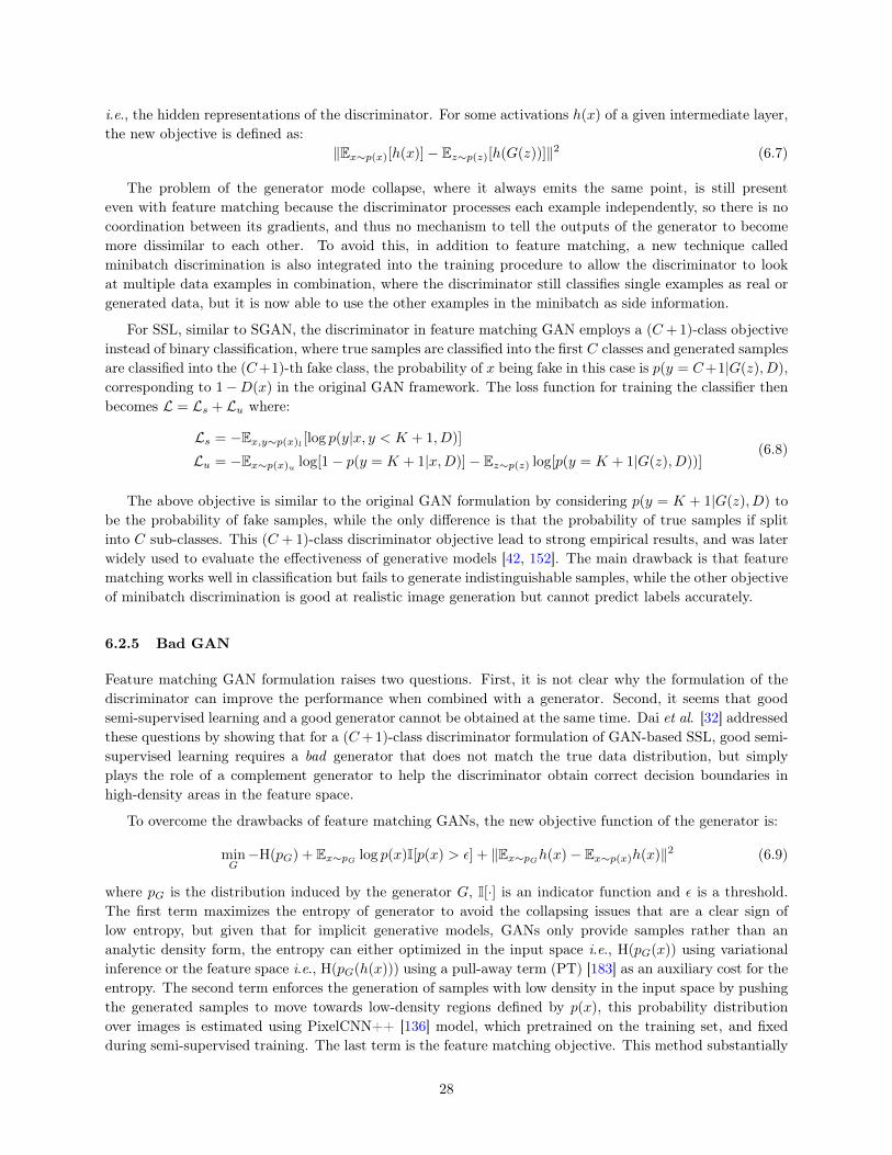
i.e., the hidden representations of the discriminator. For some activations h(x) of a given intermediate layer,the new objective is defined as:

‖Ex∼p(x)[h(x)]− Ez∼p(z)[h(G(z))]‖2 (6.7)

The problem of the generator mode collapse, where it always emits the same point, is still presenteven with feature matching because the discriminator processes each example independently, so there is nocoordination between its gradients, and thus no mechanism to tell the outputs of the generator to becomemore dissimilar to each other. To avoid this, in addition to feature matching, a new technique calledminibatch discrimination is also integrated into the training procedure to allow the discriminator to lookat multiple data examples in combination, where the discriminator still classifies single examples as real orgenerated data, but it is now able to use the other examples in the minibatch as side information.

For SSL, similar to SGAN, the discriminator in feature matching GAN employs a (C + 1)-class objectiveinstead of binary classification, where true samples are classified into the first C classes and generated samplesare classified into the (C+1)-th fake class, the probability of x being fake in this case is p(y = C+1|G(z), D),corresponding to 1−D(x) in the original GAN framework. The loss function for training the classifier thenbecomes L = Ls + Lu where:

Ls = −Ex,y∼p(x)l [log p(y|x, y < K + 1, D)]

Lu = −Ex∼p(x)u log[1− p(y = K + 1|x,D)]− Ez∼p(z) log[p(y = K + 1|G(z), D))](6.8)

The above objective is similar to the original GAN formulation by considering p(y = K + 1|G(z), D) tobe the probability of fake samples, while the only difference is that the probability of true samples if splitinto C sub-classes. This (C + 1)-class discriminator objective lead to strong empirical results, and was laterwidely used to evaluate the effectiveness of generative models [42, 152]. The main drawback is that featurematching works well in classification but fails to generate indistinguishable samples, while the other objectiveof minibatch discrimination is good at realistic image generation but cannot predict labels accurately.

6.2.5 Bad GAN

Feature matching GAN formulation raises two questions. First, it is not clear why the formulation of thediscriminator can improve the performance when combined with a generator. Second, it seems that goodsemi-supervised learning and a good generator cannot be obtained at the same time. Dai et al. [32] addressedthese questions by showing that for a (C+1)-class discriminator formulation of GAN-based SSL, good semi-supervised learning requires a bad generator that does not match the true data distribution, but simplyplays the role of a complement generator to help the discriminator obtain correct decision boundaries inhigh-density areas in the feature space.

To overcome the drawbacks of feature matching GANs, the new objective function of the generator is:

minG−H(pG) + Ex∼pG log p(x)I[p(x) > ε] + ‖Ex∼pGh(x)− Ex∼p(x)h(x)‖2 (6.9)

where pG is the distribution induced by the generator G, I[·] is an indicator function and ε is a threshold.The first term maximizes the entropy of generator to avoid the collapsing issues that are a clear sign oflow entropy, but given that for implicit generative models, GANs only provide samples rather than ananalytic density form, the entropy can either optimized in the input space i.e., H(pG(x)) using variationalinference or the feature space i.e., H(pG(h(x))) using a pull-away term (PT) [183] as an auxiliary cost for theentropy. The second term enforces the generation of samples with low density in the input space by pushingthe generated samples to move towards low-density regions defined by p(x), this probability distributionover images is estimated using PixelCNN++ [136] model, which pretrained on the training set, and fixedduring semi-supervised training. The last term is the feature matching objective. This method substantially

28

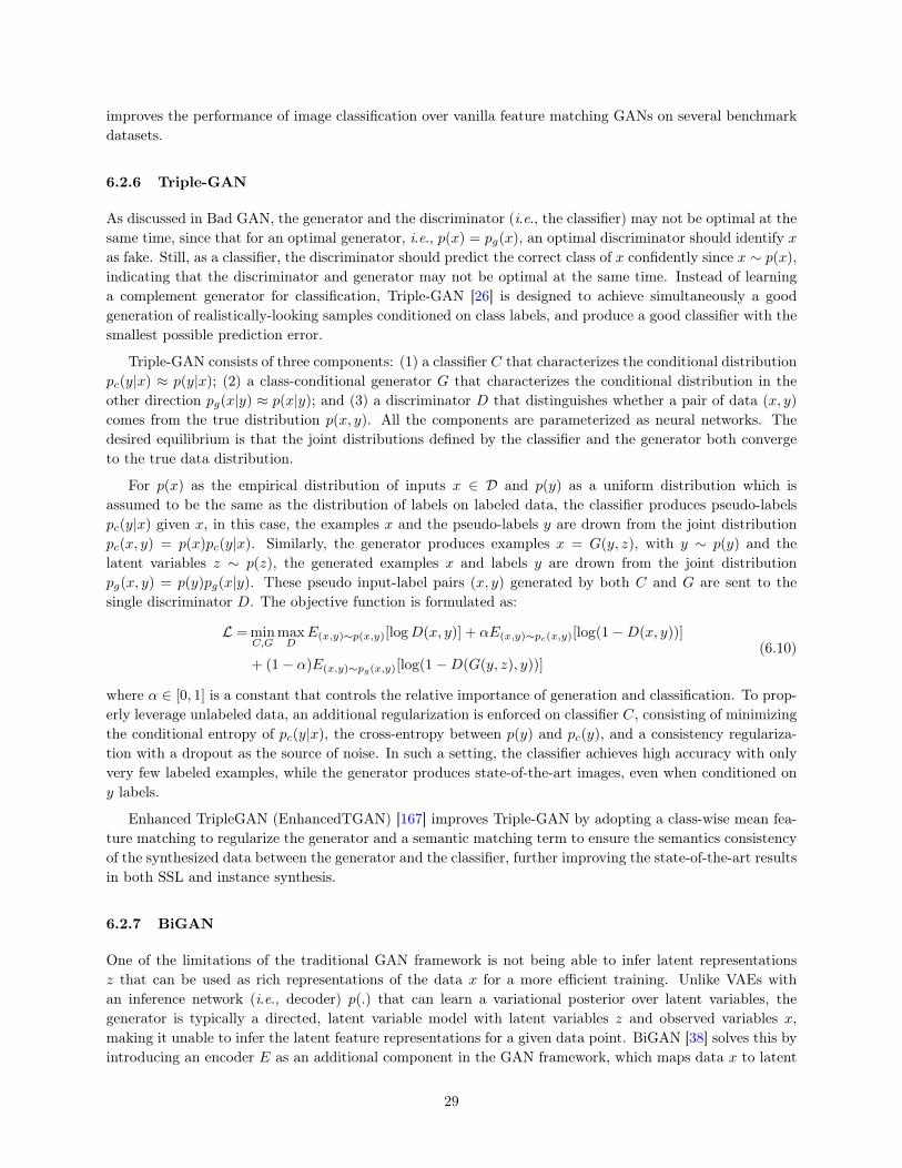
improves the performance of image classification over vanilla feature matching GANs on several benchmarkdatasets.

6.2.6 Triple-GAN

As discussed in Bad GAN, the generator and the discriminator (i.e., the classifier) may not be optimal at thesame time, since that for an optimal generator, i.e., p(x) = pg(x), an optimal discriminator should identify xas fake. Still, as a classifier, the discriminator should predict the correct class of x confidently since x ∼ p(x),indicating that the discriminator and generator may not be optimal at the same time. Instead of learninga complement generator for classification, Triple-GAN [26] is designed to achieve simultaneously a goodgeneration of realistically-looking samples conditioned on class labels, and produce a good classifier with thesmallest possible prediction error.

Triple-GAN consists of three components: (1) a classifier C that characterizes the conditional distributionpc(y|x) ≈ p(y|x); (2) a class-conditional generator G that characterizes the conditional distribution in theother direction pg(x|y) ≈ p(x|y); and (3) a discriminator D that distinguishes whether a pair of data (x, y)

comes from the true distribution p(x, y). All the components are parameterized as neural networks. Thedesired equilibrium is that the joint distributions defined by the classifier and the generator both convergeto the true data distribution.

For p(x) as the empirical distribution of inputs x ∈ D and p(y) as a uniform distribution which isassumed to be the same as the distribution of labels on labeled data, the classifier produces pseudo-labelspc(y|x) given x, in this case, the examples x and the pseudo-labels y are drown from the joint distributionpc(x, y) = p(x)pc(y|x). Similarly, the generator produces examples x = G(y, z), with y ∼ p(y) and thelatent variables z ∼ p(z), the generated examples x and labels y are drown from the joint distributionpg(x, y) = p(y)pg(x|y). These pseudo input-label pairs (x, y) generated by both C and G are sent to thesingle discriminator D. The objective function is formulated as:

L = minC,G

maxD

E(x,y)∼p(x,y)[logD(x, y)] + αE(x,y)∼pc(x,y)[log(1−D(x, y))]

+ (1− α)E(x,y)∼pg(x,y)[log(1−D(G(y, z), y))](6.10)

where α ∈ [0, 1] is a constant that controls the relative importance of generation and classification. To prop-erly leverage unlabeled data, an additional regularization is enforced on classifier C, consisting of minimizingthe conditional entropy of pc(y|x), the cross-entropy between p(y) and pc(y), and a consistency regulariza-tion with a dropout as the source of noise. In such a setting, the classifier achieves high accuracy with onlyvery few labeled examples, while the generator produces state-of-the-art images, even when conditioned ony labels.

Enhanced TripleGAN (EnhancedTGAN) [167] improves Triple-GAN by adopting a class-wise mean fea-ture matching to regularize the generator and a semantic matching term to ensure the semantics consistencyof the synthesized data between the generator and the classifier, further improving the state-of-the-art resultsin both SSL and instance synthesis.

6.2.7 BiGAN

One of the limitations of the traditional GAN framework is not being able to infer latent representationsz that can be used as rich representations of the data x for a more efficient training. Unlike VAEs withan inference network (i.e., decoder) p(.) that can learn a variational posterior over latent variables, thegenerator is typically a directed, latent variable model with latent variables z and observed variables x,making it unable to infer the latent feature representations for a given data point. BiGAN [38] solves this byintroducing an encoder E as an additional component in the GAN framework, which maps data x to latent

29

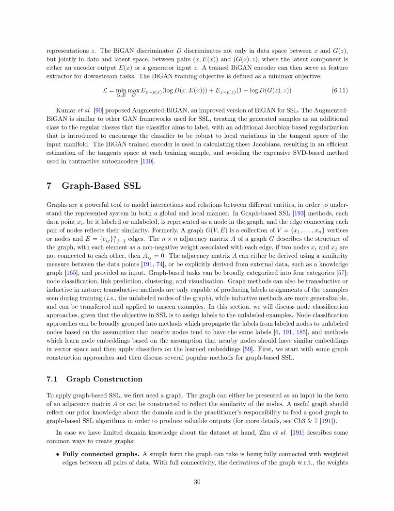
representations z. The BiGAN discriminator D discriminates not only in data space between x and G(z),but jointly in data and latent space, between pairs (x,E(x)) and (G(z), z), where the latent component iseither an encoder output E(x) or a generator input z. A trained BiGAN encoder can then serve as featureextractor for downstream tasks. The BiGAN training objective is defined as a minimax objective:

L = minG,E

maxD

Ex∼p(x)(logD(x,E(x))) + Ez∼p(z)(1− logD(G(z), z)) (6.11)

Kumar et al. [90] proposed Augmented-BiGAN, an improved version of BiGAN for SSL. The Augmented-BiGAN is similar to other GAN frameworks used for SSL, treating the generated samples as an additionalclass to the regular classes that the classifier aims to label, with an additional Jacobian-based regularizationthat is introduced to encourage the classifier to be robust to local variations in the tangent space of theinput manifold. The BiGAN trained encoder is used in calculating these Jacobians, resulting in an efficientestimation of the tangents space at each training sample, and avoiding the expensive SVD-based methodused in contractive autoencoders [130].

7 Graph-Based SSL

Graphs are a powerful tool to model interactions and relations between different entities, in order to under-stand the represented system in both a global and local manner. In Graph-based SSL [193] methods, eachdata point xi, be it labeled or unlabeled, is represented as a node in the graph, and the edge connecting eachpair of nodes reflects their similarity. Formerly, A graph G(V,E) is a collection of V = {x1, . . . , xn} verticesor nodes and E = {eij}ni,j=1 edges. The n × n adjacency matrix A of a graph G describes the structure ofthe graph, with each element as a non-negative weight associated with each edge, if two nodes xi and xj arenot connected to each other, then Aij = 0. The adjacency matrix A can either be derived using a similaritymeasure between the data points [191, 74], or be explicitly derived from external data, such as a knowledgegraph [165], and provided as input. Graph-based tasks can be broadly categorized into four categories [57]:node classification, link prediction, clustering, and visualization. Graph methods can also be transductive orinductive in nature; transductive methods are only capable of producing labels assignments of the examplesseen during training (i.e., the unlabeled nodes of the graph), while inductive methods are more generalizable,and can be transferred and applied to unseen examples. In this section, we will discuss node classificationapproaches, given that the objective in SSL is to assign labels to the unlabeled examples. Node classificationapproaches can be broadly grouped into methods which propagate the labels from labeled nodes to unlabelednodes based on the assumption that nearby nodes tend to have the same labels [6, 191, 185], and methodswhich learn node embeddings based on the assumption that nearby nodes should have similar embeddingsin vector space and then apply classifiers on the learned embeddings [59]. First, we start with some graphconstruction approaches and then discuss several popular methods for graph-based SSL.

7.1 Graph Construction

To apply graph-based SSL, we first need a graph. The graph can either be presented as an input in the formof an adjacency matrix A or can be constructed to reflect the similarity of the nodes. A useful graph shouldreflect our prior knowledge about the domain and is the practitioner’s responsibility to feed a good graph tograph-based SSL algorithms in order to produce valuable outputs (for more details, see Ch3 & 7 [191]).

In case we have limited domain knowledge about the dataset at hand, Zhu et al. [191] describes somecommon ways to create graphs:

• Fully connected graphs. A simple form the graph can take is being fully connected with weightededges between all pairs of data. With full connectivity, the derivatives of the graph w.r.t., the weights

30

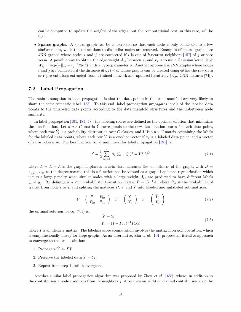
can be computed to update the weights of the edges, but the computational cost, in this case, will behigh.

• Sparse graphs. A sparse graph can be constructed so that each node is only connected to a fewsimilar nodes, while the connections to dissimilar nodes are removed. Examples of sparse graphs arekNN graphs where nodes i and j are connected if i is one of k-nearest neighbors [157] of j or viceversa. A possible way to obtain the edge weight Aij between xi and xj is to use a Gaussian kernel [15]:Wij = exp{−‖xi−xj‖2/2σ2} with a hyperparameter σ. Another approach is εNN graphs where nodesi and j are connected if the distance d(i, j) ≤ ε. These graphs can be created using either the raw dataor representations extracted from a trained network and updated iteratively (e.g., CNN features [74]).

7.2 Label Propagation

The main assumption in label propagation is that the data points in the same manifold are very likely toshare the same semantic label [185]. To this end, label propagation propagates labels of the labeled datapoints to the unlabeled data points according to the data manifold structures and the in-between nodesimilarity.

In label propagation [191, 185, 48], the labeling scores are defined as the optimal solution that minimizesthe loss function. Let a n × C matrix Y corresponds to the new classification scores for each data point,where each row Yi is a probability distribution over C classes, and Y is a n×C matrix containing the labelsfor the labeled data points, where each row Yi is a one-hot vector if xi is a labeled data point, and a vectorof zeros otherwise. The loss function to be minimized for label propagation [191] is:

L =1

2

n∑i,j=1

Aij(yi − yj)2 = Y TLY (7.1)

where L = D − A is the graph Laplacian matrix that measures the smoothness of the graph, with D =∑nj=1Aij as the degree matrix, this loss function can be viewed as a graph Laplacian regularization which

incurs a large penalty when similar nodes with a large weight Aij are predicted to have different labelsyi 6= yj . By defining a n × n probabilistic transition matrix P = D−1A, where Pij is the probability oftransit from node i to j, and spliting the matrices P , Y and Y into labeled and unlabeled sub-matrices:

P =

(Pll PluPul Puu

)Y =

(YlYu

)Y =

(YlYu

)(7.2)

the optimal solution for eq. (7.1) is:Yl = Yl

Yu = (I − Puu)−1PulYl(7.3)

where I is an identity matrix. The labeling score computation involves the matrix inversion operation, whichis computationally heavy for large graphs. As an alternative, Zhu et al. [191] propose an iterative approachto converge to the same solution:

1. Propagate Y ← PY .

2. Preserve the labeled data Yl = Yl.

3. Repeat from step 1 until convergence.

Another similar label propagation algorithm was proposed by Zhou et al. [185], where, in addition tothe contribution a node i receives from its neighbors j, it receives an additional small contribution given by

31

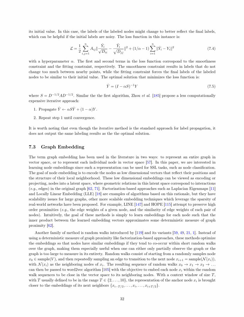
its initial value. In this case, the labels of the labeled nodes might change to better reflect the final labels,which can be helpful if the initial labels are noisy. The loss function in this instance is:

L =1

2

n∑i,j=1

Aij‖Yi√Dii

− Yi√Djj

‖2 + (1/α− 1)

n∑i=1

‖Yi − Yi‖2 (7.4)

with a hyperparameter α. The first and second terms in the loss function correspond to the smoothnessconstraint and the fitting constraint, respectively. The smoothness constraint results in labels that do notchange too much between nearby points, while the fitting constraint forces the final labels of the labelednodes to be similar to their initial value. The optimal solution that minimizes the loss function is:

Y = (I − αS)−1Y (7.5)

where S = D−1/2AD−1/2. Similar the the first algorithm, Zhou et al. [185] propose a less computationallyexpensive iterative approach:

1. Propagate Y ← αSY + (1− α)Y .

2. Repeat step 1 until convergence.

It is worth noting that even though the iterative method is the standard approach for label propagation, itdoes not output the same labeling results as the the optimal solution.

7.3 Graph Embedding

The term graph embedding has been used in the literature in two ways: to represent an entire graph invector space, or to represent each individual node in vector space [57]. In this paper, we are interested inlearning node embeddings since such a representation can be used for SSL tasks, such as node classification.The goal of node embedding is to encode the nodes as low dimensional vectors that reflect their positions andthe structure of their local neighborhood. These low dimensional embeddings can be viewed as encoding orprojecting, nodes into a latent space, where geometric relations in this latent space correspond to interactions(e.g., edges) in the original graph [62, 71]. Factorization-based approaches such as Laplacian Eigenmaps [11]and Locally Linear Embedding (LLE) [18] are examples of algorithms based on this rationale, but they havescalability issues for large graphs, other more scalable embedding techniques which leverage the sparsity ofreal-world networks have been proposed. For example, LINE [147] and HOPE [115] attempt to preserve highorder proximities (e.g., the edge weights of a given node, and the similarity of edge weights of each pair ofnodes). Intuitively, the goal of these methods is simply to learn embeddings for each node such that theinner product between the learned embedding vectors approximates some deterministic measure of graphproximity [62].

Another family of method is random walks introduced by [119] and its variants [59, 49, 21, 1]. Instead ofusing a deterministic measure of graph proximity like factorization-based approaches, these methods optimizethe embeddings so that nodes have similar embeddings if they tend to co-occur within short random walksover the graph, making them especially useful when one can either only partially observe the graph or thegraph is too large to measure in its entirety. Random walks consist of starting from a randomly samples nodex0 ∈ sample(V ), and then repeatedly sampling an edge to transition to the next node xi+1 = sample(N (xi)),with N (xi) as the neighboring nodes of xi. The resulting sequence of random walks x0 → x1 → x2 → . . .

can then be passed to word2vec algorithm [105] with the objective to embed each node xi within the randomwalk sequences to be close in the vector space to its neighboring nodes. With a context window of size T ,with T usually defined to be in the range T ∈ {2, . . . , 10}, the representation of the anchor node xi is broughtcloser to the embeddings of its next neighbors {xi−T/2, . . . , xi, . . . , xi+T/2}.

32

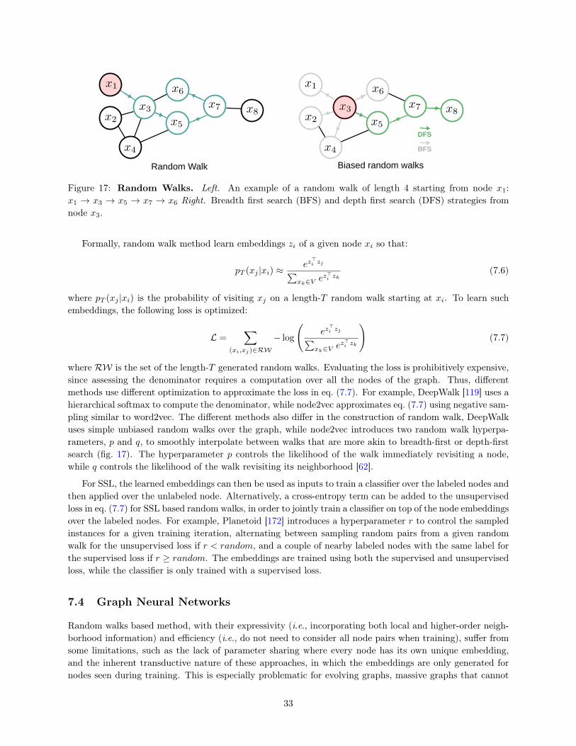
Random Walk Biased random walks

DFS

BFS

Figure 17: Random Walks. Left. An example of a random walk of length 4 starting from node x1:x1 → x3 → x5 → x7 → x6 Right. Breadth first search (BFS) and depth first search (DFS) strategies fromnode x3.

Formally, random walk method learn embeddings zi of a given node xi so that:

pT (xj |xi) ≈ez

>i zj∑

xk∈V ez>i zk

(7.6)

where pT (xj |xi) is the probability of visiting xj on a length-T random walk starting at xi. To learn suchembeddings, the following loss is optimized:

L =∑

(xi,xj)∈RW

− log

(ez

>i zj∑

xk∈V ez>i zk

)(7.7)

where RW is the set of the length-T generated random walks. Evaluating the loss is prohibitively expensive,since assessing the denominator requires a computation over all the nodes of the graph. Thus, differentmethods use different optimization to approximate the loss in eq. (7.7). For example, DeepWalk [119] uses ahierarchical softmax to compute the denominator, while node2vec approximates eq. (7.7) using negative sam-pling similar to word2vec. The different methods also differ in the construction of random walk, DeepWalkuses simple unbiased random walks over the graph, while node2vec introduces two random walk hyperpa-rameters, p and q, to smoothly interpolate between walks that are more akin to breadth-first or depth-firstsearch (fig. 17). The hyperparameter p controls the likelihood of the walk immediately revisiting a node,while q controls the likelihood of the walk revisiting its neighborhood [62].

For SSL, the learned embeddings can then be used as inputs to train a classifier over the labeled nodes andthen applied over the unlabeled node. Alternatively, a cross-entropy term can be added to the unsupervisedloss in eq. (7.7) for SSL based random walks, in order to jointly train a classifier on top of the node embeddingsover the labeled nodes. For example, Planetoid [172] introduces a hyperparameter r to control the sampledinstances for a given training iteration, alternating between sampling random pairs from a given randomwalk for the unsupervised loss if r < random, and a couple of nearby labeled nodes with the same label forthe supervised loss if r ≥ random. The embeddings are trained using both the supervised and unsupervisedloss, while the classifier is only trained with a supervised loss.

7.4 Graph Neural Networks

Random walks based method, with their expressivity (i.e., incorporating both local and higher-order neigh-borhood information) and efficiency (i.e., do not need to consider all node pairs when training), suffer fromsome limitations, such as the lack of parameter sharing where every node has its own unique embedding,and the inherent transductive nature of these approaches, in which the embeddings are only generated fornodes seen during training. This is especially problematic for evolving graphs, massive graphs that cannot

33

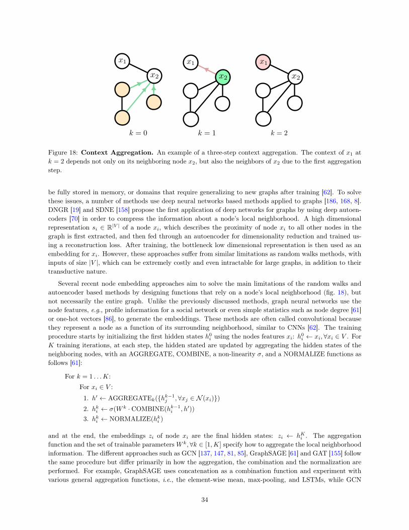
Figure 18: Context Aggregation. An example of a three-step context aggregation. The context of x1 atk = 2 depends not only on its neighboring node x2, but also the neighbors of x2 due to the first aggregationstep.

be fully stored in memory, or domains that require generalizing to new graphs after training [62]. To solvethese issues, a number of methods use deep neural networks based methods applied to graphs [186, 168, 8].DNGR [19] and SDNE [158] propose the first application of deep networks for graphs by using deep autoen-coders [70] in order to compress the information about a node’s local neighborhood. A high dimensionalrepresentation si ∈ R|V | of a node xi, which describes the proximity of node xi to all other nodes in thegraph is first extracted, and then fed through an autoencoder for dimensionality reduction and trained us-ing a reconstruction loss. After training, the bottleneck low dimensional representation is then used as anembedding for xi. However, these approaches suffer from similar limitations as random walks methods, withinputs of size |V |, which can be extremely costly and even intractable for large graphs, in addition to theirtransductive nature.

Several recent node embedding approaches aim to solve the main limitations of the random walks andautoencoder based methods by designing functions that rely on a node’s local neighborhood (fig. 18), butnot necessarily the entire graph. Unlike the previously discussed methods, graph neural networks use thenode features, e.g., profile information for a social network or even simple statistics such as node degree [61]or one-hot vectors [86], to generate the embeddings. These methods are often called convolutional becausethey represent a node as a function of its surrounding neighborhood, similar to CNNs [62]. The trainingprocedure starts by initializing the first hidden states h0i using the nodes features xi: h0i ← xi,∀xi ∈ V . ForK training iterations, at each step, the hidden stated are updated by aggregating the hidden states of theneighboring nodes, with an AGGREGATE, COMBINE, a non-linearity σ, and a NORMALIZE functions asfollows [61]:

For k = 1 . . .K:

For xi ∈ V :

1. h′ ← AGGREGATEk({hk−1j ,∀xj ∈ N (xi)})2. hki ← σ(W k · COMBINE(hk−1i , h′))

3. hki ← NORMALIZE(hki )

and at the end, the embeddings zi of node xi are the final hidden states: zi ← hKi . The aggregationfunction and the set of trainable parametersW k,∀k ∈ [1,K] specify how to aggregate the local neighborhoodinformation. The different approaches such as GCN [137, 147, 81, 85], GraphSAGE [61] and GAT [155] followthe same procedure but differ primarily in how the aggregation, the combination and the normalization areperformed. For example, GraphSAGE uses concatenation as a combination function and experiment withvarious general aggregation functions, i.e., the element-wise mean, max-pooling, and LSTMs, while GCN

34

uses a weighted sum as a combination function and element-wise mean as an aggregate. The weight are thentrained using an unsupervised loss similar to random walks based methods, and for SSL [85], a classifier istrained on top of the node embeddings (i.e., the final hidden state) to predict the class labels for the labelednodes, which can then applied on the unlabeled nodes for node classification.

8 Self-Supervision for SSL

Self-supervised learning [163, 76] is a form of unsupervised learning, where the model is trained using astandard supervised loss, but on a pretext task where the supervision comes from the data itself. Theobjective, in this case, is not to maximize final performance on the pretext task, but rather to learn richand transferable features for downstream tasks. A variety of pretext tasks were proposed, where the modelis first trained on one or multiple tasks with unlabeled examples, the resulting model is either used forgenerating representations for the raw data, which are utilized for training a shallow classifier on Dl, ordirectly fine-tuned for a downstream task with labeled images. Examples of such pretext tasks for computervision are:

• Exemplar-CNN [40]. For a given image, a set of N patches are generated using different transfor-mations, all these patches are then considered as a separate class, and the model is trained to predictthe correct class for a given input patch.

• Rotation [53]. A given rotation out of four possible rotations of multiple of 90◦, i.e., [0◦, 90◦, 180◦, 270◦],is applied to the input image, and the model is trained to predict the correct rotation that was applied.

• Patches [37]. A first patch is randomly extracted from the input image, this patch is considered as thecenter, and eight different neighboring and non-overlapping patches are extracted with small jitters atthe eight neighboring locations, the model is then trained to predict the position of one of the secondpatches with regard to the first one. Other versions of this pretext task were proposed, such as jigsawpuzzle [111] where a random permutation of the nine patches are fed into the model, and the objectiveis to predict the correct permutation that was applied to get the correct ordering of the patches.

• Colorization [179]. The input image is first transformed from RGB to Lab color space, an input withonly the luminance information contained within the L component or the color information with abcomponents is fed into the model, and the objective is to predict the rest of the information, i.e., eitherthe luminance or the coloring of the image. The task can either be considered as a regression problemor a classification problem by quantizing the Lab color space.

• Contrastive Predictive Coding [114]. Using a contrastive loss based on Noise Contrastive Esti-mation [60] and its recent versions such as Momentum Contrast [66] and SimCLR [22], the modelis trained to differentiate between positive and negative samples, the positives can be a given inputimage and its transformed versions, or a given patch and its neighboring patches, while the negativesare randomly sampled images or patches.

Such pretext tasks can easily be utilized for SSL, where the model is trained on the whole dataset on thepretext task with self-supervision, and then adapted to the labeled set Dl using the standard cross-entropyloss, either simultaneously as demonstrated by [175, 12] with rotation as the pretext task, or iteratively, byfirst training the model using self-supervision and then fine tuning it on Dl as demonstrated by [22, 23] usingcontrastive learning.

35

9 Conclusion

In this paper, we introduced semi-supervised learning, with its main approaches and assumptions, withSSL techniques within deep learning framework. Specifically, this review covered four broad categories ofapproaches for SSL: consistency regularization, generative models, graph-based methods, and holistic ap-proaches. With the growing research interest in data-efficient deep learning algorithms, it is foreseeable thatdeep SSL methods could approach the performance of fully supervised methods, and have board applicationsintegrated into different systems and learning paradigms.

Acknowledgements

Y. Ouali is supported by Randstad corporate research in collaboration with Université Paris-Saclay, Cen-traleSupélec, MICS. We thank Victor Bouvier for his helpful feedback on an earlier version.

References[1] Sami Abu-El-Haija, Bryan Perozzi, Rami Al-Rfou, and Alexander A Alemi. Watch your step: Learning node embeddings

via graph attention. In Advances in Neural Information Processing Systems, pages 9180–9190, 2018.

[2] Eric Arazo, Diego Ortego, Paul Albert, Noel E O’Connor, and Kevin McGuinness. Pseudo-labeling and confirmation biasin deep semi-supervised learning. arXiv preprint arXiv:1908.02983, 2019.

[3] Ehsan Mohammady Ardehaly and Aron Culotta. Co-training for demographic classification using deep learning fromlabel proportions. In 2017 IEEE International Conference on Data Mining Workshops (ICDMW), pages 1017–1024.IEEE, 2017.

[4] Martin Arjovsky, Soumith Chintala, and Léon Bottou. Wasserstein gan. arXiv preprint arXiv:1701.07875, 2017.

[5] Ben Athiwaratkun, Marc Finzi, Pavel Izmailov, and Andrew Gordon Wilson. There are many consistent explanations ofunlabeled data: Why you should average. arXiv preprint arXiv:1806.05594, 2018.

[6] Arik Azran. The rendezvous algorithm: Multiclass semi-supervised learning with markov random walks. In Proceedingsof the 24th international conference on Machine learning, pages 49–56, 2007.

[7] Yauhen Babakhin, Artsiom Sanakoyeu, and Hirotoshi Kitamura. Semi-supervised segmentation of salt bodies in seismicimages using an ensemble of convolutional neural networks. In German Conference on Pattern Recognition, pages 218–231. Springer, 2019.

[8] Davide Bacciu, Federico Errica, Alessio Micheli, and Marco Podda. A gentle introduction to deep learning for graphs.arXiv preprint arXiv:1912.12693, 2019.

[9] Amy Bearman, Olga Russakovsky, Vittorio Ferrari, and Li Fei-Fei. What’s the point: Semantic segmentation with pointsupervision. In European conference on computer vision, pages 549–565. Springer, 2016.

[10] Oscar Beijbom. Domain adaptations for computer vision applications. arXiv preprint arXiv:1211.4860, 2012.

[11] Mikhail Belkin and Partha Niyogi. Laplacian eigenmaps and spectral techniques for embedding and clustering. InAdvances in neural information processing systems, pages 585–591, 2002.

[12] David Berthelot, Nicholas Carlini, Ekin D Cubuk, Alex Kurakin, Kihyuk Sohn, Han Zhang, and Colin Raffel. Remixmatch:Semi-supervised learning with distribution alignment and augmentation anchoring. arXiv preprint arXiv:1911.09785,2019.

[13] David Berthelot, Nicholas Carlini, Ian Goodfellow, Nicolas Papernot, Avital Oliver, and Colin A Raffel. Mixmatch: Aholistic approach to semi-supervised learning. In Advances in Neural Information Processing Systems, pages 5050–5060,2019.

[14] Christian Biemann. Unsupervised and knowledge-free natural language processing in the structure discovery paradigm.PhD thesis, Leipzig University, Germany, 2007.

[15] Christopher M Bishop. Pattern recognition and machine learning. springer, 2006.

[16] Avrim Blum and Tom Mitchell. Combining labeled and unlabeled data with co-training. In Proceedings of the eleventhannual conference on Computational learning theory, pages 92–100, 1998.

[17] Leo Breiman. Randomizing outputs to increase prediction accuracy. Machine Learning, 40(3):229–242, 2000.

36

[18] Shaosheng Cao, Wei Lu, and Qiongkai Xu. Grarep: Learning graph representations with global structural information.In Proceedings of the 24th ACM international on conference on information and knowledge management, pages 891–900,2015.

[19] Shaosheng Cao, Wei Lu, and Qiongkai Xu. Deep neural networks for learning graph representations. In Thirtieth AAAIconference on artificial intelligence, 2016.

[20] Olivier Chapelle, Bernhard Scholkopf, and Alexander Zien. Semi-supervised learning (chapelle, o. et al., eds.; 2006)[bookreviews]. IEEE Transactions on Neural Networks, 20(3):542–542, 2009.

[21] Haochen Chen, Bryan Perozzi, Yifan Hu, and Steven Skiena. Harp: Hierarchical representation learning for networks. InThirty-Second AAAI Conference on Artificial Intelligence, 2018.

[22] Ting Chen, Simon Kornblith, Mohammad Norouzi, and Geoffrey Hinton. A simple framework for contrastive learning ofvisual representations. arXiv preprint arXiv:2002.05709, 2020.

[23] Ting Chen, Simon Kornblith, Kevin Swersky, Mohammad Norouzi, and Geoffrey Hinton. Big self-supervised models arestrong semi-supervised learners. arXiv preprint arXiv:2006.10029, 2020.

[24] Yanhua Cheng, Xin Zhao, Rui Cai, Zhiwei Li, Kaiqi Huang, Yong Rui, et al. Semi-supervised multimodal deep learningfor rgb-d object recognition. 2016.

[25] Yong Cheng. Semi-supervised learning for neural machine translation. In Joint Training for Neural Machine Translation,pages 25–40. Springer, 2019.

[26] LI Chongxuan, Taufik Xu, Jun Zhu, and Bo Zhang. Triple generative adversarial nets. In Advances in neural informationprocessing systems, pages 4088–4098, 2017.

[27] Kevin Clark, Minh-Thang Luong, Christopher D Manning, and Quoc V Le. Semi-supervised sequence modeling withcross-view training. arXiv preprint arXiv:1809.08370, 2018.

[28] Martin Cooke, Phil Green, Ljubomir Josifovski, and Ascension Vizinho. Robust automatic speech recognition with missingand unreliable acoustic data. Speech communication, 34(3):267–285, 2001.

[29] Ekin D Cubuk, Barret Zoph, Dandelion Mane, Vijay Vasudevan, and Quoc V Le. Autoaugment: Learning augmentationstrategies from data. In Proceedings of the IEEE conference on computer vision and pattern recognition, pages 113–123,2019.

[30] Ekin D Cubuk, Barret Zoph, Jonathon Shlens, and Quoc V Le. Randaugment: Practical data augmentation with noseparate search. arXiv preprint arXiv:1909.13719, 2019.

[31] Jifeng Dai, Kaiming He, and Jian Sun. Boxsup: Exploiting bounding boxes to supervise convolutional networks forsemantic segmentation. 2015 IEEE International Conference on Computer Vision (ICCV), Dec 2015.

[32] Zihang Dai, Zhilin Yang, Fan Yang, William W Cohen, and Russ R Salakhutdinov. Good semi-supervised learning thatrequires a bad gan. In Advances in neural information processing systems, pages 6510–6520, 2017.

[33] Sanjoy Dasgupta. Analysis of a greedy active learning strategy. In Advances in neural information processing systems,pages 337–344, 2005.

[34] Jia Deng, Wei Dong, Richard Socher, Li-Jia Li, Kai Li, and Li Fei-Fei. Imagenet: A large-scale hierarchical imagedatabase. In 2009 IEEE conference on computer vision and pattern recognition, pages 248–255. Ieee, 2009.

[35] Yifan Ding, Liqiang Wang, Deliang Fan, and Boqing Gong. A semi-supervised two-stage approach to learning from noisylabels. In 2018 IEEE Winter Conference on Applications of Computer Vision (WACV), pages 1215–1224. IEEE, 2018.

[36] Carl Doersch. Tutorial on variational autoencoders. arXiv preprint arXiv:1606.05908, 2016.

[37] Carl Doersch, Abhinav Gupta, and Alexei A Efros. Unsupervised visual representation learning by context prediction.In Proceedings of the IEEE international conference on computer vision, pages 1422–1430, 2015.

[38] Jeff Donahue, Philipp Krähenbühl, and Trevor Darrell. Adversarial feature learning. arXiv preprint arXiv:1605.09782,2016.

[39] WeiWang Dong-DongChen and Zhi-HuaZhou WeiGao. Tri-net for semi-supervised deep learning. In Proceedings ofTwenty-Seventh International Joint Conference on Artificial Intelligence, pages 2014–2020, 2018.

[40] Alexey Dosovitskiy, Philipp Fischer, Jost Tobias Springenberg, Martin Riedmiller, and Thomas Brox. Discriminativeunsupervised feature learning with exemplar convolutional neural networks. IEEE transactions on pattern analysis andmachine intelligence, 38(9):1734–1747, 2015.

[41] Thomas Drugman, Janne Pylkkonen, and Reinhard Kneser. Active and semi-supervised learning in asr: Benefits on theacoustic and language models. arXiv preprint arXiv:1903.02852, 2019.

[42] Vincent Dumoulin, Ishmael Belghazi, Ben Poole, Olivier Mastropietro, Alex Lamb, Martin Arjovsky, and Aaron Courville.Adversarially learned inference. arXiv preprint arXiv:1606.00704, 2016.

37

[43] Sergey Edunov, Myle Ott, Michael Auli, and David Grangier. Understanding back-translation at scale. arXiv preprintarXiv:1808.09381, 2018.

[44] M Ehsan Abbasnejad, Anthony Dick, and Anton van den Hengel. Infinite variational autoencoder for semi-supervisedlearning. In Proceedings of the IEEE Conference on Computer Vision and Pattern Recognition, pages 5888–5897, 2017.

[45] Dennis Forster, Abdul-Saboor Sheikh, and Jörg Lücke. Neural simpletrons: Learning in the limit of few labels withdirected generative networks. Neural computation, 30(8):2113–2174, 2018.

[46] Benoît Frénay and Michel Verleysen. Classification in the presence of label noise: a survey. IEEE transactions on neuralnetworks and learning systems, 25(5):845–869, 2013.

[47] Geoffrey French, Michal Mackiewicz, and Mark Fisher. Self-ensembling for visual domain adaptation. arXiv preprintarXiv:1706.05208, 2017.

[48] Yasuhiro Fujiwara and Go Irie. Efficient label propagation. In International Conference on Machine Learning, pages784–792, 2014.

[49] Soumyajit Ganguly, Manish Gupta, Vasudeva Varma, Vikram Pudi, et al. Author2vec: Learning author representationsby combining content and link information. In Proceedings of the 25th International Conference Companion on WorldWide Web, pages 49–50. International World Wide Web Conferences Steering Committee, 2016.

[50] Yaroslav Ganin and Victor Lempitsky. Unsupervised domain adaptation by backpropagation. arXiv preprintarXiv:1409.7495, 2014.

[51] Mingfei Gao, Zizhao Zhang, Guo Yu, Sercan O Arik, Larry S Davis, and Tomas Pfister. Consistency-based semi-supervisedactive learning: Towards minimizing labeling cost. arXiv preprint arXiv:1910.07153, 2019.

[52] Salvador García, Julián Luengo, and Francisco Herrera. Data preprocessing in data mining. Springer, 2015.

[53] Spyros Gidaris, Praveer Singh, and Nikos Komodakis. Unsupervised representation learning by predicting image rotations.arXiv preprint arXiv:1803.07728, 2018.

[54] Chen Gong, Dacheng Tao, Wei Liu, Liu Liu, and Jie Yang. Label propagation via teaching-to-learn and learning-to-teach.IEEE transactions on neural networks and learning systems, 28(6):1452–1465, 2016.

[55] Ian Goodfellow, Jean Pouget-Abadie, Mehdi Mirza, Bing Xu, David Warde-Farley, Sherjil Ozair, Aaron Courville, andYoshua Bengio. Generative adversarial nets. In Advances in neural information processing systems, pages 2672–2680,2014.

[56] Ian J Goodfellow, Jonathon Shlens, and Christian Szegedy. Explaining and harnessing adversarial examples. arXivpreprint arXiv:1412.6572, 2014.

[57] Palash Goyal and Emilio Ferrara. Graph embedding techniques, applications, and performance: A survey. Knowledge-Based Systems, 151:78–94, 2018.

[58] Yves Grandvalet and Yoshua Bengio. Semi-supervised learning by entropy minimization. In Advances in neural infor-mation processing systems, pages 529–536, 2005.

[59] Aditya Grover and Jure Leskovec. node2vec: Scalable feature learning for networks. In Proceedings of the 22nd ACMSIGKDD international conference on Knowledge discovery and data mining, pages 855–864, 2016.

[60] Michael Gutmann and Aapo Hyvärinen. Noise-contrastive estimation: A new estimation principle for unnormalizedstatistical models. In Proceedings of the Thirteenth International Conference on Artificial Intelligence and Statistics,pages 297–304, 2010.

[61] Will Hamilton, Zhitao Ying, and Jure Leskovec. Inductive representation learning on large graphs. In Advances in neuralinformation processing systems, pages 1024–1034, 2017.

[62] William L Hamilton, Rex Ying, and Jure Leskovec. Representation learning on graphs: Methods and applications. arXivpreprint arXiv:1709.05584, 2017.

[63] Steve Hanneke. Theoretical foundations of active learning. Technical report, CARNEGIE-MELLON UNIV PITTS-BURGH PA MACHINE LEARNING DEPT, 2009.

[64] Di He, Yingce Xia, Tao Qin, Liwei Wang, Nenghai Yu, Tie-Yan Liu, and Wei-Ying Ma. Dual learning for machinetranslation. In Advances in neural information processing systems, pages 820–828, 2016.

[65] Junxian He, Jiatao Gu, Jiajun Shen, and Marc’Aurelio Ranzato. Revisiting self-training for neural sequence generation.arXiv preprint arXiv:1909.13788, 2019.

[66] Kaiming He, Haoqi Fan, Yuxin Wu, Saining Xie, and Ross Girshick. Momentum contrast for unsupervised visual repre-sentation learning. arXiv preprint arXiv:1911.05722, 2019.

[67] Kaiming He, Xiangyu Zhang, Shaoqing Ren, and Jian Sun. Deep residual learning for image recognition. In Proceedingsof the IEEE conference on computer vision and pattern recognition, pages 770–778, 2016.

38

[68] Dan Hendrycks and Thomas Dietterich. Benchmarking neural network robustness to common corruptions and perturba-tions. arXiv preprint arXiv:1903.12261, 2019.

[69] Dan Hendrycks, Norman Mu, Ekin D Cubuk, Barret Zoph, Justin Gilmer, and Balaji Lakshminarayanan. Augmix: Asimple data processing method to improve robustness and uncertainty. arXiv preprint arXiv:1912.02781, 2019.

[70] Geoffrey E Hinton and Ruslan R Salakhutdinov. Reducing the dimensionality of data with neural networks. science,313(5786):504–507, 2006.

[71] Peter D Hoff, Adrian E Raftery, and Mark S Handcock. Latent space approaches to social network analysis. Journal ofthe american Statistical association, 97(460):1090–1098, 2002.

[72] Sheng-Jun Huang, Rong Jin, and Zhi-Hua Zhou. Active learning by querying informative and representative examples.In Advances in neural information processing systems, pages 892–900, 2010.

[73] Sergey Ioffe and Christian Szegedy. Batch normalization: Accelerating deep network training by reducing internal covariateshift. arXiv preprint arXiv:1502.03167, 2015.

[74] Ahmet Iscen, Giorgos Tolias, Yannis Avrithis, and Ondrej Chum. Label propagation for deep semi-supervised learning.In Proceedings of the IEEE Conference on Computer Vision and Pattern Recognition, pages 5070–5079, 2019.

[75] Pavel Izmailov, Dmitrii Podoprikhin, Timur Garipov, Dmitry Vetrov, and Andrew Gordon Wilson. Averaging weightsleads to wider optima and better generalization. arXiv preprint arXiv:1803.05407, 2018.

[76] Longlong Jing and Yingli Tian. Self-supervised visual feature learning with deep neural networks: A survey. arXivpreprint arXiv:1902.06162, 2019.

[77] Thorsten Joachims. Transductive inference for text classification using support vector machines. In Icml, volume 99,pages 200–209, 1999.

[78] Thorsten Joachims. Transductive learning via spectral graph partitioning. In Proceedings of the 20th InternationalConference on Machine Learning (ICML-03), pages 290–297, 2003.

[79] Giannis Karamanolakis, Daniel Hsu, and Luis Gravano. Leveraging just a few keywords for fine-grained aspect detectionthrough weakly supervised co-training. arXiv preprint arXiv:1909.00415, 2019.

[80] Zhanghan Ke, Daoye Wang, Qiong Yan, Jimmy Ren, and Rynson WH Lau. Dual student: Breaking the limits of theteacher in semi-supervised learning. In Proceedings of the IEEE International Conference on Computer Vision, pages6728–6736, 2019.

[81] Steven Kearnes, Kevin McCloskey, Marc Berndl, Vijay Pande, and Patrick Riley. Molecular graph convolutions: movingbeyond fingerprints. Journal of computer-aided molecular design, 30(8):595–608, 2016.

[82] Diederik P Kingma and Jimmy Ba. Adam: A method for stochastic optimization. arXiv preprint arXiv:1412.6980, 2014.

[83] Diederik P Kingma and Max Welling. Auto-encoding variational bayes. arXiv preprint arXiv:1312.6114, 2013.

[84] Durk P Kingma, Shakir Mohamed, Danilo Jimenez Rezende, and Max Welling. Semi-supervised learning with deepgenerative models. In Advances in neural information processing systems, pages 3581–3589, 2014.

[85] Thomas N Kipf and Max Welling. Semi-supervised classification with graph convolutional networks. arXiv preprintarXiv:1609.02907, 2016.

[86] Thomas N Kipf and Max Welling. Variational graph auto-encoders. arXiv preprint arXiv:1611.07308, 2016.

[87] Kyeongbo Kong, Junggi Lee, Youngchul Kwak, Minsung Kang, Seong Gyun Kim, and Woo-Jin Song. Recycling: Semi-supervised learning with noisy labels in deep neural networks. IEEE Access, 7:66998–67005, 2019.

[88] Alex Krizhevsky, Geoffrey Hinton, et al. Learning multiple layers of features from tiny images. 2009.

[89] Abhishek Kumar and Hal Daumé. A co-training approach for multi-view spectral clustering. In Proceedings of the 28thinternational conference on machine learning (ICML-11), pages 393–400, 2011.

[90] Abhishek Kumar, Prasanna Sattigeri, and Tom Fletcher. Semi-supervised learning with gans: Manifold invariance withimproved inference. In Advances in Neural Information Processing Systems, pages 5534–5544, 2017.

[91] Abhishek Kumar, Prasanna Sattigeri, Kahini Wadhawan, Leonid Karlinsky, Rogerio Feris, Bill Freeman, and GregoryWornell. Co-regularized alignment for unsupervised domain adaptation. In Advances in Neural Information ProcessingSystems, pages 9345–9356, 2018.

[92] Samuli Laine and Timo Aila. Temporal ensembling for semi-supervised learning. arXiv preprint arXiv:1610.02242, 2016.

[93] Dong-Hyun Lee. Pseudo-label: The simple and efficient semi-supervised learning method for deep neural networks. InWorkshop on challenges in representation learning, ICML, volume 3, page 2, 2013.

[94] Jungbeom Lee, Eunji Kim, Sungmin Lee, Jangho Lee, and Sungroh Yoon. Ficklenet: Weakly and semi-supervisedsemantic image segmentation\\using stochastic inference. arXiv preprint arXiv:1902.10421, 2019.

39

[95] Seungmin Lee, Dongwan Kim, Namil Kim, and Seong-Gyun Jeong. Drop to adapt: Learning discriminative featuresfor unsupervised domain adaptation. In Proceedings of the IEEE International Conference on Computer Vision, pages91–100, 2019.

[96] Junnan Li, Richard Socher, and Steven CH Hoi. Dividemix: Learning with noisy labels as semi-supervised learning.arXiv preprint arXiv:2002.07394, 2020.

[97] Kunpeng Li, Ziyan Wu, Kuan-Chuan Peng, Jan Ernst, and Yun Fu. Tell me where to look: Guided attention inferencenetwork. 2018 IEEE/CVF Conference on Computer Vision and Pattern Recognition, Jun 2018.

[98] Xinzhe Li, Qianru Sun, Yaoyao Liu, Qin Zhou, Shibao Zheng, Tat-Seng Chua, and Bernt Schiele. Learning to self-trainfor semi-supervised few-shot classification. In Advances in Neural Information Processing Systems, pages 10276–10286,2019.

[99] Jae Hyun Lim and Jong Chul Ye. Geometric gan. arXiv preprint arXiv:1705.02894, 2017.

[100] Di Lin, Jifeng Dai, Jiaya Jia, Kaiming He, and Jian Sun. Scribblesup: Scribble-supervised convolutional networks forsemantic segmentation. In Proceedings of the IEEE Conference on Computer Vision and Pattern Recognition, pages3159–3167, 2016.

[101] Xingjun Ma, Yisen Wang, Michael E Houle, Shuo Zhou, Sarah M Erfani, Shu-Tao Xia, Sudanthi Wijewickrema, andJames Bailey. Dimensionality-driven learning with noisy labels. arXiv preprint arXiv:1806.02612, 2018.

[102] Lars Maaløe, Casper Kaae Sønderby, Søren Kaae Sønderby, and Ole Winther. Auxiliary deep generative models. arXivpreprint arXiv:1602.05473, 2016.

[103] Andrew L Maas, Raymond E Daly, Peter T Pham, Dan Huang, Andrew Y Ng, and Christopher Potts. Learning wordvectors for sentiment analysis. In Proceedings of the 49th annual meeting of the association for computational linguistics:Human language technologies-volume 1, pages 142–150. Association for Computational Linguistics, 2011.

[104] Christoph Mayer, Matthieu Paul, and Radu Timofte. Adversarial feature distribution alignment for semi-supervisedlearning. arXiv preprint arXiv:1912.10428, 2019.

[105] Tomas Mikolov, Ilya Sutskever, Kai Chen, Greg S Corrado, and Jeff Dean. Distributed representations of words andphrases and their compositionality. In Advances in neural information processing systems, pages 3111–3119, 2013.

[106] Mike Mintz, Steven Bills, Rion Snow, and Dan Jurafsky. Distant supervision for relation extraction without labeled data.In Proceedings of the Joint Conference of the 47th Annual Meeting of the ACL and the 4th International Joint Conferenceon Natural Language Processing of the AFNLP: Volume 2-Volume 2, pages 1003–1011. Association for ComputationalLinguistics, 2009.

[107] Takeru Miyato, Toshiki Kataoka, Masanori Koyama, and Yuichi Yoshida. Spectral normalization for generative adversarialnetworks. arXiv preprint arXiv:1802.05957, 2018.

[108] Takeru Miyato, Shin-ichi Maeda, Masanori Koyama, and Shin Ishii. Virtual adversarial training: a regularization methodfor supervised and semi-supervised learning. IEEE transactions on pattern analysis and machine intelligence, 41(8):1979–1993, 2018.

[109] Todd K Moon. The expectation-maximization algorithm. IEEE Signal processing magazine, 13(6):47–60, 1996.

[110] Yuval Netzer, Tao Wang, Adam Coates, Alessandro Bissacco, Bo Wu, and Andrew Y Ng. Reading digits in naturalimages with unsupervised feature learning. 2011.

[111] Mehdi Noroozi and Paolo Favaro. Unsupervised learning of visual representations by solving jigsaw puzzles. In EuropeanConference on Computer Vision, pages 69–84. Springer, 2016.

[112] Augustus Odena. Semi-supervised learning with generative adversarial networks. arXiv preprint arXiv:1606.01583, 2016.

[113] Avital Oliver, Augustus Odena, Colin A Raffel, Ekin Dogus Cubuk, and Ian Goodfellow. Realistic evaluation of deepsemi-supervised learning algorithms. In Advances in Neural Information Processing Systems, pages 3235–3246, 2018.

[114] Aaron van den Oord, Yazhe Li, and Oriol Vinyals. Representation learning with contrastive predictive coding. arXivpreprint arXiv:1807.03748, 2018.

[115] Mingdong Ou, Peng Cui, Jian Pei, Ziwei Zhang, and Wenwu Zhu. Asymmetric transitivity preserving graph embedding.In Proceedings of the 22nd ACM SIGKDD international conference on Knowledge discovery and data mining, pages1105–1114, 2016.

[116] Sinno Jialin Pan and Qiang Yang. A survey on transfer learning. IEEE Transactions on knowledge and data engineering,22(10):1345–1359, 2009.

[117] Sungrae Park, JunKeon Park, Su-Jin Shin, and Il-Chul Moon. Adversarial dropout for supervised and semi-supervisedlearning. In Thirty-Second AAAI Conference on Artificial Intelligence, 2018.

[118] Vishal M Patel, Raghuraman Gopalan, Ruonan Li, and Rama Chellappa. Visual domain adaptation: A survey of recentadvances. IEEE signal processing magazine, 32(3):53–69, 2015.

40

[119] Bryan Perozzi, Rami Al-Rfou, and Steven Skiena. Deepwalk: Online learning of social representations. In Proceedings ofthe 20th ACM SIGKDD international conference on Knowledge discovery and data mining, pages 701–710, 2014.

[120] Hieu Pham, Qizhe Xie, Zihang Dai, and Quoc V Le. Meta pseudo labels. arXiv preprint arXiv:2003.10580, 2020.

[121] Siyuan Qiao, Wei Shen, Zhishuai Zhang, Bo Wang, and Alan Yuille. Deep co-training for semi-supervised image recogni-tion. In Proceedings of the european conference on computer vision (eccv), pages 135–152, 2018.

[122] Joaquin Quionero-Candela, Masashi Sugiyama, Anton Schwaighofer, and Neil D Lawrence. Dataset shift in machinelearning. The MIT Press, 2009.

[123] Alec Radford, Luke Metz, and Soumith Chintala. Unsupervised representation learning with deep convolutional generativeadversarial networks. arXiv preprint arXiv:1511.06434, 2015.

[124] Rajesh Ranganath, Dustin Tran, and David Blei. Hierarchical variational models. In International Conference on MachineLearning, pages 324–333, 2016.

[125] Antti Rasmus, Mathias Berglund, Mikko Honkala, Harri Valpola, and Tapani Raiko. Semi-supervised learning with laddernetworks. In Advances in neural information processing systems, pages 3546–3554, 2015.

[126] Alex Ratner, P Varma, B Hancock, and Chris Ré. Weak supervision: A new programming paradigm for machine learning(2019).

[127] Scott Reed, Honglak Lee, Dragomir Anguelov, Christian Szegedy, Dumitru Erhan, and Andrew Rabinovich. Trainingdeep neural networks on noisy labels with bootstrapping. arXiv preprint arXiv:1412.6596, 2014.

[128] Danilo Jimenez Rezende, Shakir Mohamed, and Daan Wierstra. Stochastic backpropagation and approximate inferencein deep generative models. arXiv preprint arXiv:1401.4082, 2014.

[129] Phill Kyu Rhee, Enkhbayar Erdenee, Shin Dong Kyun, Minhaz Uddin Ahmed, and Songguo Jin. Active and semi-supervised learning for object detection with imperfect data. Cognitive Systems Research, 45:109–123, 2017.

[130] Salah Rifai, Yann N Dauphin, Pascal Vincent, Yoshua Bengio, and Xavier Muller. The manifold tangent classifier. InAdvances in neural information processing systems, pages 2294–2302, 2011.

[131] Ellen Riloff. Automatically generating extraction patterns from untagged text. In Proceedings of the national conferenceon artificial intelligence, pages 1044–1049, 1996.

[132] Ellen Riloff and Janyce Wiebe. Learning extraction patterns for subjective expressions. In Proceedings of the 2003conference on Empirical methods in natural language processing, pages 105–112, 2003.

[133] Sebastian Ruder and Barbara Plank. Strong baselines for neural semi-supervised learning under domain shift. arXivpreprint arXiv:1804.09530, 2018.

[134] Kuniaki Saito, Yoshitaka Ushiku, and Tatsuya Harada. Asymmetric tri-training for unsupervised domain adaptation. InProceedings of the 34th International Conference on Machine Learning-Volume 70, pages 2988–2997. JMLR. org, 2017.

[135] Tim Salimans, Ian Goodfellow, Wojciech Zaremba, Vicki Cheung, Alec Radford, and Xi Chen. Improved techniques fortraining gans. In Advances in neural information processing systems, pages 2234–2242, 2016.

[136] Tim Salimans, Andrej Karpathy, Xi Chen, and Diederik P Kingma. Pixelcnn++: Improving the pixelcnn with discretizedlogistic mixture likelihood and other modifications. arXiv preprint arXiv:1701.05517, 2017.

[137] Franco Scarselli, Marco Gori, Ah Chung Tsoi, Markus Hagenbuchner, and Gabriele Monfardini. The graph neural networkmodel. IEEE Transactions on Neural Networks, 20(1):61–80, 2008.

[138] H Scudder. Probability of error of some adaptive pattern-recognition machines. IEEE Transactions on InformationTheory, 11(3):363–371, 1965.

[139] Rico Sennrich, Barry Haddow, and Alexandra Birch. Improving neural machine translation models with monolingualdata. arXiv preprint arXiv:1511.06709, 2015.

[140] Burr Settles. Active learning literature survey. Technical report, University of Wisconsin-Madison Department of Com-puter Sciences, 2009.

[141] Weiwei Shi, Yihong Gong, Chris Ding, Zhiheng MaXiaoyu Tao, and Nanning Zheng. Transductive semi-superviseddeep learning using min-max features. In Proceedings of the European Conference on Computer Vision (ECCV), pages299–315, 2018.

[142] Rui Shu, Hung H Bui, Hirokazu Narui, and Stefano Ermon. A dirt-t approach to unsupervised domain adaptation. arXivpreprint arXiv:1802.08735, 2018.

[143] Kihyuk Sohn, David Berthelot, Chun-Liang Li, Zizhao Zhang, Nicholas Carlini, Ekin D Cubuk, Alex Kurakin, HanZhang, and Colin Raffel. Fixmatch: Simplifying semi-supervised learning with consistency and confidence. arXiv preprintarXiv:2001.07685, 2020.

[144] Chunfeng Song, Yan Huang, Wanli Ouyang, and Liang Wang. Box-driven class-wise region masking and filling rate guidedloss for weakly supervised semantic segmentation, 2019.

41

[145] Jost Tobias Springenberg. Unsupervised and semi-supervised learning with categorical generative adversarial networks.arXiv preprint arXiv:1511.06390, 2015.

[146] Mingxing Tan and Quoc V Le. Efficientnet: Rethinking model scaling for convolutional neural networks. arXiv preprintarXiv:1905.11946, 2019.

[147] Jian Tang, Meng Qu, Mingzhe Wang, Ming Zhang, Jun Yan, and Qiaozhu Mei. Line: Large-scale information networkembedding. In Proceedings of the 24th international conference on world wide web, pages 1067–1077, 2015.

[148] Antti Tarvainen and Harri Valpola. Mean teachers are better role models: Weight-averaged consistency targets improvesemi-supervised deep learning results. In Advances in neural information processing systems, pages 1195–1204, 2017.

[149] Sunil Thulasidasan, Tanmoy Bhattacharya, Jeff Bilmes, Gopinath Chennupati, and Jamal Mohd-Yusof. Combating labelnoise in deep learning using abstention. arXiv preprint arXiv:1905.10964, 2019.

[150] Jonathan Tompson, Ross Goroshin, Arjun Jain, Yann LeCun, and Christoph Bregler. Efficient object localization usingconvolutional networks. In Proceedings of the IEEE Conference on Computer Vision and Pattern Recognition, pages648–656, 2015.

[151] Dustin Tran, Rajesh Ranganath, and David M Blei. Deep and hierarchical implicit models. arXiv preprintarXiv:1702.08896, 7:3, 2017.

[152] Dmitry Ulyanov, Andrea Vedaldi, and Victor Lempitsky. It takes (only) two: Adversarial generator-encoder networks.In Thirty-Second AAAI Conference on Artificial Intelligence, 2018.

[153] Harri Valpola. From neural pca to deep unsupervised learning. In Advances in independent component analysis andlearning machines, pages 143–171. Elsevier, 2015.

[154] Andreas Veit, Neil Alldrin, Gal Chechik, Ivan Krasin, Abhinav Gupta, and Serge Belongie. Learning from noisy large-scaledatasets with minimal supervision. In Proceedings of the IEEE Conference on Computer Vision and Pattern Recognition,pages 839–847, 2017.

[155] Petar Veličković, Guillem Cucurull, Arantxa Casanova, Adriana Romero, Pietro Lio, and Yoshua Bengio. Graph attentionnetworks. arXiv preprint arXiv:1710.10903, 2017.

[156] Vikas Verma, Alex Lamb, Juho Kannala, Yoshua Bengio, and David Lopez-Paz. Interpolation consistency training forsemi-supervised learning. arXiv preprint arXiv:1903.03825, 2019.

[157] Ulrike Von Luxburg. A tutorial on spectral clustering. Statistics and computing, 17(4):395–416, 2007.

[158] Daixin Wang, Peng Cui, and Wenwu Zhu. Structural deep network embedding. In Proceedings of the 22nd ACM SIGKDDinternational conference on Knowledge discovery and data mining, pages 1225–1234, 2016.

[159] Xiang Wang, Shaodi You, Xi Li, and Huimin Ma. Weakly-Supervised Semantic Segmentation by Iteratively MiningCommon Object Features. Proceedings of the IEEE Computer Society Conference on Computer Vision and PatternRecognition, pages 1354–1362, 2018.

[160] Zhengxia Wang, Xiaofeng Zhu, Ehsan Adeli, Yingying Zhu, Chen Zu, Feiping Nie, Dinggang Shen, and Guorong Wu.Progressive graph-based transductive learning for multi-modal classification of brain disorder disease. In InternationalConference on Medical Image Computing and Computer-Assisted Intervention, pages 291–299. Springer, 2016.

[161] Yunchao Wei, Huaxin Xiao, Honghui Shi, Zequn Jie, Jiashi Feng, and Thomas S. Huang. Revisiting dilated convolution:A simple approach for weakly- and semi-supervised semantic segmentation. 2018 IEEE/CVF Conference on ComputerVision and Pattern Recognition, Jun 2018.

[162] Karl Weiss, Taghi M Khoshgoftaar, and DingDing Wang. A survey of transfer learning. Journal of Big data, 3(1):9, 2016.

[163] Lilian Weng. Self-supervised representation learning. lilianweng.github.io/lil-log, 2019.

[164] Max Whitney and Anoop Sarkar. Bootstrapping via graph propagation. In Proceedings of the 50th Annual Meeting ofthe Association for Computational Linguistics: Long Papers-Volume 1, pages 620–628. Association for ComputationalLinguistics, 2012.

[165] Derry Wijaya, Partha Pratim Talukdar, and Tom Mitchell. Pidgin: ontology alignment using web text as interlingua. InProceedings of the 22nd ACM international conference on Information & Knowledge Management, pages 589–598, 2013.

[166] Garrett Wilson and Diane J Cook. A survey of unsupervised deep domain adaptation. arXiv preprint arXiv:1812.02849,2018.

[167] Si Wu, Guangchang Deng, Jichang Li, Rui Li, Zhiwen Yu, and Hau-San Wong. Enhancing triplegan for semi-supervisedconditional instance synthesis and classification. In Proceedings of the IEEE Conference on Computer Vision and PatternRecognition, pages 10091–10100, 2019.

[168] Zonghan Wu, Shirui Pan, Fengwen Chen, Guodong Long, Chengqi Zhang, and S Yu Philip. A comprehensive survey ongraph neural networks. IEEE Transactions on Neural Networks and Learning Systems, 2020.

[169] Qizhe Xie, Zihang Dai, Eduard Hovy, Minh-Thang Luong, and Quoc V Le. Unsupervised data augmentation for consis-tency training. 2019.

42

[170] Qizhe Xie, Eduard Hovy, Minh-Thang Luong, and Quoc V Le. Self-training with noisy student improves imagenetclassification. arXiv preprint arXiv:1911.04252, 2019.

[171] I Zeki Yalniz, Hervé Jégou, Kan Chen, Manohar Paluri, and Dhruv Mahajan. Billion-scale semi-supervised learning forimage classification. arXiv preprint arXiv:1905.00546, 2019.

[172] Zhilin Yang, William W Cohen, and Ruslan Salakhutdinov. Revisiting semi-supervised learning with graph embeddings.arXiv preprint arXiv:1603.08861, 2016.

[173] David Yarowsky. Unsupervised word sense disambiguation rivaling supervised methods. In 33rd annual meeting of theassociation for computational linguistics, pages 189–196, 1995.

[174] Kun Yi and Jianxin Wu. Probabilistic end-to-end noise correction for learning with noisy labels. In Proceedings of theIEEE Conference on Computer Vision and Pattern Recognition, pages 7017–7025, 2019.

[175] Xiaohua Zhai, Avital Oliver, Alexander Kolesnikov, and Lucas Beyer. S4l: Self-supervised semi-supervised learning. InProceedings of the IEEE international conference on computer vision, pages 1476–1485, 2019.

[176] Han Zhang, Ian Goodfellow, Dimitris Metaxas, and Augustus Odena. Self-attention generative adversarial networks.arXiv preprint arXiv:1805.08318, 2018.

[177] Han Zhang, Zizhao Zhang, Augustus Odena, and Honglak Lee. Consistency regularization for generative adversarialnetworks. arXiv preprint arXiv:1910.12027, 2019.

[178] Hongyi Zhang, Moustapha Cisse, Yann N Dauphin, and David Lopez-Paz. mixup: Beyond empirical risk minimization.arXiv preprint arXiv:1710.09412, 2017.

[179] Richard Zhang, Phillip Isola, and Alexei A Efros. Colorful image colorization. In European conference on computervision, pages 649–666. Springer, 2016.

[180] Xiang Zhang, Junbo Zhao, and Yann LeCun. Character-level convolutional networks for text classification. In Advancesin neural information processing systems, pages 649–657, 2015.

[181] Yan-Ming Zhang, Kaizhu Huang, and Cheng-Lin Liu. Fast and robust graph-based transductive learning via minimumtree cut. In 2011 IEEE 11th International Conference on Data Mining, pages 952–961. IEEE, 2011.

[182] Jing Zhao, Xijiong Xie, Xin Xu, and Shiliang Sun. Multi-view learning overview: Recent progress and new challenges.Information Fusion, 38:43–54, 2017.

[183] Junbo Zhao, Michael Mathieu, and Yann LeCun. Energy-based generative adversarial network. arXiv preprintarXiv:1609.03126, 2016.

[184] Bolei Zhou, Aditya Khosla, Agata Lapedriza, Aude Oliva, and Antonio Torralba. Learning deep features for discriminativelocalization. 2016 IEEE Conference on Computer Vision and Pattern Recognition (CVPR), Jun 2016.

[185] Dengyong Zhou, Olivier Bousquet, Thomas N Lal, Jason Weston, and Bernhard Schölkopf. Learning with local and globalconsistency. In Advances in neural information processing systems, pages 321–328, 2004.

[186] Jie Zhou, Ganqu Cui, Zhengyan Zhang, Cheng Yang, Zhiyuan Liu, Lifeng Wang, Changcheng Li, and Maosong Sun.Graph neural networks: A review of methods and applications. arXiv preprint arXiv:1812.08434, 2018.

[187] Yan Zhou and Sally Goldman. Democratic co-learning. In 16th IEEE International Conference on Tools with ArtificialIntelligence, pages 594–602. IEEE, 2004.

[188] Zhi-Hua Zhou. A brief introduction to weakly supervised learning. National Science Review, 5(1):44–53, 2018.

[189] Zhi-Hua Zhou and Ming Li. Tri-training: Exploiting unlabeled data using three classifiers. IEEE Transactions onknowledge and Data Engineering, 17(11):1529–1541, 2005.

[190] Xiaojin Zhu and Zoubin Ghahramani. Learning from labeled and unlabeled data with label propagation. 2002.

[191] Xiaojin Zhu, Zoubin Ghahramani, and John D Lafferty. Semi-supervised learning using gaussian fields and harmonicfunctions. In Proceedings of the 20th International conference on Machine learning (ICML-03), pages 912–919, 2003.

[192] Xiaojin Zhu, John Lafferty, and Zoubin Ghahramani. Combining active learning and semi-supervised learning usinggaussian fields and harmonic functions. In ICML 2003 workshop on the continuum from labeled to unlabeled data inmachine learning and data mining, volume 3, 2003.

[193] Xiaojin Jerry Zhu. Semi-supervised learning literature survey. Technical report, University of Wisconsin-Madison De-partment of Computer Sciences, 2005.

43