Repairable systems as stochastic processes

Barbara Russo

Reference }  Michael Baron Probability and statistics for computer

scientists }  Chapter 6

Stochastic processes types }  Discrete/con+nuous    in  +me    

}  Xω(t)  can  be  discrete  or  con+nuous  }  The  process  is  +me  con+nuous  or  +me  discrete  

}  Fixing  ω,  X  ω(t)  is  called  a  path  

}  Discrete/con+nuous  in  output    }  X  t(ω)  can  be  discrete  or  con+nuous  }  The  process  is  state  con+nuous  or  state  discrete  

Example }  Number of an output o after n tosses X(n,o)

}  n tosses of a coin }  {1,..., n} = observations =time }  {head, tail} = outputs The values of X(n,o) are called states X(3,head) n=3 and o=head. We do not know ex-ante the value of

X(3,head); we know it once we observe the three tosses, but we can discuss the probability of X(3,head)

Example (source Baron) }  Internet connections }  X(t,n)= total number of connections by time t

}  Continuous in time (any moment a connection can happen) }  Discrete in number of connections

}  Exercise. find an example in computer science of all possible combinations discrete/continuous random variables

Markov processes }  A Markov process is a stochastic process whose future

behaviour depends only on present }  The behaviour is described by the conditional probability

that an event happens }  P{future| present and past}=P{future | present}

}  Example Internet connections }  The future total number of internet connections depend on

the present total number of connections disregarding what were the connections in the past

Markov chain }  A MC is a time and state discrete Markov process }  It parameterises the set of outputs with the finite or

countable sets }  It defines the transition probability matrix

}  P(t): pij (t)= P{X(t+1)=j| X(t)=i}

}  More in general the transition probability matrix after h steps (observations) P(t+h):

}  pij h(t)= P{X(t+h)=j| X(t)=i} }  A MC is homogeneous if all the transition probability

matrices are independent of t à }  pij (t)= pij and pij h(t)= pij h

The distribution of a MC }  The distribution of the MC is completely determined by

the initial value at time 0 of the probability }  P0(x)=(X(0)=x) for x ranging all the possible output values }  and the one step transition probabilities pij

}  Law of Total Probability

}  In our case

}  And since in a MC

}  then

Example }  Compute probability that in two steps three defects

occur }  P(2)

03=P{X(2)=3|X(0)=0}

The transition diagrams and the stochastic matrix at one step

}  Example P does not depend on step

}  Properties: for every i

1 2

p11 p12

p21

p22

Using Markov chain in failure count }  Assumptions:

}  We model the cumulative number of failures }  If we assume no reparation process within the interval of

observation otherwise stated => some path are not feasible (you cannot go back)

Method to derive the Markov chain }  We identify the set of outputs

}  The set contains all the possible values of all the states. }  So if an intermediate state has the highest number of defects

we need to take that as maximum values of our output set. }  In failures count, as we consider cumulative number of failures

the last state contains always the maximum.

}  Draw the graph of states connected by the probabilities of going to one state to another and to remain in the same state.

}  The graph is called transition diagram

The transition diagram }  pij=Probability that the future state is j when the past

state was i

}  Output set= {1,2}

1 2

p11 p12

p21

p22

Transition diagrams }  Positive probabilities tell us that we can move from one state

to another one }  Probability zero tells there is no link in the corresponding

direction }  The matrix P has

}  rows saying probabilities to move from the state of value = “row number” to any future value. Summing up the row values we get 1, as we are summing up on all the possible future outputs conditioned to a specific past state.

}  columns describing all the conditions of the past states of a given future state. Summing up the column entries we get the unconditioned probability of the future state

}  Remember that in our assumptions states are independent: one cannot have at the same instant k and j failures if k is different from j

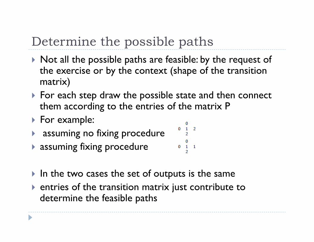
Determine the possible paths }  Not all the possible paths are feasible: by the request of

the exercise or by the context (shape of the transition matrix)

}  For each step draw the possible state and then connect them according to the entries of the matrix P

}  For example: }  assuming no fixing procedure }  assuming fixing procedure

}  In the two cases the set of outputs is the same }  entries of the transition matrix just contribute to

determine the feasible paths

Assuming bug fixing }  A process that is declared with no fixing procedure needs

to have a P matrix that has zeros in the entries that would allow the move from greater number of failures (from 3 to 2 for example it should be p32=0), but

}  It is always possible to ask for computing the probability over those paths not to have a fixing procedure. }  In this case the matrix P can have non zero entries for moves

from a greater number of failures but we just do not consider these entries in the probability computation

Absorbing states }  P describe the geometry of the MC process and defines

the path you want to describe }  Thee can be some special states or zones called

absorbing states or zones }  A MC is regular if pij (h)>0 for some h and every i and j }  When there is a state i with pii =1 the transition matrix P

cannot be regular. Namely: }  pii=I => pij=0 for every j not = i => (P(h))ij =Pij for all h

}  Such state is called absorbing there is no exit from state i

Exercise }  Suppose a point process of cumulative failure

occurrences is defined by a Markov Chain of four states with transition matrix

¨  P=

}  Compute the total probability of passing from 0 to 3 failures in exactly three steps of the process. Draw the graphical representation of the process.

}  The exercise is equivalent to determine P303 (?)

2/16/103/14/14/14/14/13/13/13/102/15/16/130/4

Exercise }  Baron’s book pg 153 }  A computer is shared by 2 users who work

independently. }  At any minute:

}  Connected user can disconnect with P=0.5 }  Disconnected user can connect with P = 0.2

}  X(t) the number of connected users at time t }  We rephrase the exercise assuming a fixing

process in two failing components }  p1= probability that a reliable component fails }  p2= probability that a failed component is

repaired

Discuss the Markov chain process: Solution

}  There are three states = {0,1,2} corresponding to 0 components reliable, 1 component reliable, 2 components reliable }  Set (a,b) the components, one can have (0,0),(1,0),(0,1), (1,1)

states }  So the probability is defined passing from one state (a,b) to

another state (a’,b’)

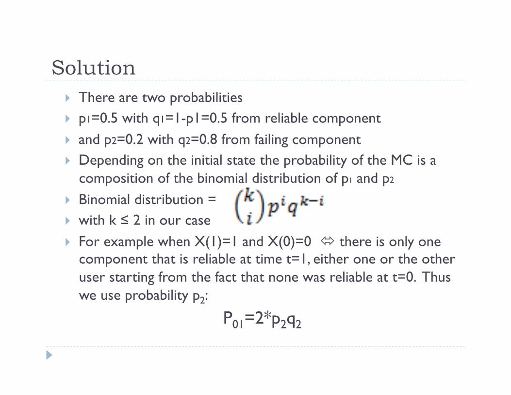
Solution }  There are two probabilities }  p1=0.5 with q1=1-p1=0.5 from reliable component }  and p2=0.2 with q2=0.8 from failing component }  Depending on the initial state the probability of the MC is a

composition of the binomial distribution of p1 and p2

}  Binomial distribution = }  with k ≤ 2 in our case }  For example when X(1)=1 and X(0)=0 ó there is only one

component that is reliable at time t=1, either one or the other user starting from the fact that none was reliable at t=0. Thus we use probability p2:

P01=2*p2q2

Note Binomial process }  X(n) is the number of successes in n independent Bernulli

trials }  Exercise a binomial process is a MC. }  X(n) = number of successes in n trials = }  p = probability of success in a trial p=P(1) and probability of

unsuccess q=1-p =P(0) }  Probability of k successes in n trials

}  P(k)=P(X(n)=k)=

}  P(X(n)<= k)=sumk P(k)

nk

!

"#

$

%& pkqn−k

}  Assume X(0)=0 }  Depending on the initial state one has a different binomial probability

describing the conditional probability p0i

}  Assuming X(0)=1 }  ..... }  Assuming X(0)=2 }  ... we build the transition matrix P }  The situation is equal in every instant of time }  we build the MC for more than one step just using the tansition

formula for more than one step Pn

Finally ...the MC is defined with The probability mass function of the MC is at the end given

by The last equality corrects the one in the Baron’s book (not

correct)

Counting processes }  A stochastic process is counting if the X(t) is the number

of items counted by time t }  The random counting variable defines a counting process

Markov Models }  Powerful techniques to analyse complex probabilistic

systems, based on the notion of states and transitions between states

}  Abstract the system into a set of mutually exclusive system states }  For example a combination of working and failed modules of

the system }  A Markov chain is a a set of equations describing the

probabilistic transitions from one state to the next one and an initial probability distribution in the state of the process

Comment on time continuous stochastic processes

}  Processes continuous in time can be discretised. }  Example. Internet connections }  The stochastic process is continuous in time but if we fix a set

of instances in which we observe the total number of connections the process becomes discrete in time