THE 5th STUDENT SYMPOSIUM ON MECHANICAL AND MANUFACTURING ENGINEERING

Sensorless Control of a Hub Mounted Switched Reluctance Motor

A. B. Kjaer, A. D. Krogsdal, E. H. Nielsen, F. M. Nielsen, S. Korsgaard, S. P. Moeller

Department of Materials and Production, Aalborg UniversityFibigerstraede 16, DK-9220 Aalborg East, Denmark

Email: fmni13@student.aau.dk,Web page: http://www.mechman.m-tech.aau.dk/

AbstractThis paper covers sensorless control by the use of a flux linkage/current method, applied on a single phase doubleU-core switched reluctance machine (SRM). This problem is stated by Johnson Controls, that has shown interest inthis type of motor and control strategy for an Ultra Short Axial Compressor (USAC). The SRM technology concept isbriefly described, and a dynamic model of the system is derived. The dynamic simulation model of the SRM systemtakes inputs from three finite element analysis (FEA) look-up tables, which describes the magnetisation curves, torqueand core loss characteristics of the SRM prototype. The SRM is operated through an inverter, which is connectedto a digital signal processor (DSP) through an interface board. This board and inverter used for communication ofthe SRM are designed for this specific motor. The motor is initially tested with a standard feedback control methodwith position and speed feedback from a Hall sensor, where controllers for speed and current control are designed.Sensorless estimation of position and speed is developed for the SRM prototype based on flux linkage and currentFEA. Testing yielded reasonable results with regards to speed estimation, but showed a 20 % error in the positionestimation. The sensorless feedback was not used for closed loop control.

Keywords: Sensorless Control, Switched Reluctance Motor, Double U-core, Inverter, Multi Stage Cooling System

1. IntroductionThe motivation for studying sensorless control of ahub mounted single phase double U-core SRM is, thatJohnson Controls has patented a multi stage coolingsystem with five SRMs called a USAC, where someproblems arise with respect to position feedback due toa harsh environment of operation. This system differsfrom the system that Johnson Controls has used inthe past, since that system had an external inductionmotor, which drove seven impellers. However, forenvironmental reasons this system was redesigned inorder to avoid the use of toxic refrigerants, and insteadutilise water. By introducing these hub mounted SRMs,problems arise as encoders or Hall sensor are notsuitable for the operation environment of the USAC, andthis leads to the interest in applying sensorless control.

The working principle of an SRM is utilisation of thefact that the rotor always moves towards the positionswith the least reluctance, and thereby the highestinductance, when a current is induced in the coils [1],and this relation is described in equation (1).

L =N2

R(1)

Here, L is the inductance, R is the reluctance, and N is

the number of windings in each coil. The SRM utilisesthe double U-core technology, where the flux path isshorter than for classic types of SRMs. This short fluxpath is illustrated in Fig. 1, and the U-core developmentis described and patented in [2].

Fig. 1 Illustration of the SRM and U-core technology. Greypart is the rotor, while the yellow part is the stator. The redarrows show the flux paths.

1

The double U-core is developed and described in [3].The main advantages for implementing the double U-core SRM are:

• No permanent magnets are needed, which reducescosts and is more environmentally sound [4].

• Shorter flux path, which decreases the core lossesand thereby increases the efficiency.

• Single phase motor which makes it easier tocontrol.

• Since windings are only present on the stator, thereare no copper losses on the rotor.

The main focus of this paper is to investigate thepossibility of using sensorless position estimation, tocontrol the SRM. The final design of the SRM was givenfrom the project start as well as the FEA look-up tables.An exploded view of the SRM can be seen in Fig. 2.

Impeller

Stator

Axle

RotorLaminations

End plates

Fig. 2 Exploded view of the SRM, where the maincomponents are presented.

2. Dynamic ModelTo simulate the dynamic response of the SRM, anonlinear model is derived. An overview of the modelis seen in Fig. 4 The voltage equation is derived fromKirchhoff’s Voltage Law, and Newtons II Law forrotational motion is used to establish the mechanicalmodel.

The voltage drop in the electrical system is expressed in

equation 2. This equation contains a resistance voltagedrop, an inductance voltage drop and a voltage drop dueto the back-emf. However, as this equation includes thederivatives of the inductance as a function of the rotorposition, the inductance must be known for all rotorpositions. Therefore, FEA look-up tables are utilisedas these provide an approximation of the inductanceas a function of the current and rotor position. Indexi denotes the considered coil.

ui = Ri(T ) ii + Lidiidt

+∂Li∂θ

∂θ

dtii (2)

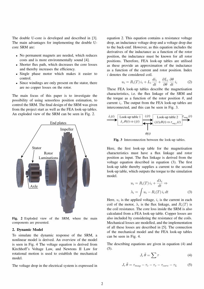
These FEA look-up tables describe the magnetisationcharacteristics, i.e. the flux linkage of the SRM andthe torque as a function of the rotor position θ, andcurrent ii. The output from the FEA look-up tables areinterconnected, and this can be seen in Fig. 3.

( )i tλ ( )ii tLook-up table 1

θ(t)

mag, ( )i tτ, ( ) ( )i it i tλ θ ⇒

Look-up table 2

,( ), ( ) ( )i mag ii t t tθ τ⇒

Fig. 3 Interconnection between the look-up tables.

Here, the first look-up table for the magnetisationcharacteristics must have a flux linkage and rotorposition as input. The flux linkage is derived from thevoltage equation described in equation (3). The firstlook-up table thereby supplies a current to the secondlook-up table, which outputs the torque to the simulationmodel.

ui = Ri(T ) ii +dλidt⇒

λi =

∫ui −Ri(T ) ii dt (3)

Here, ui is the applied voltage, ii is the current in eachcoil of the motor, λi is the flux linkage, and Ri(T ) isthe coil resistance. The core loss inside the SRM is alsocalculated from a FEA look-up table. Copper losses arealso included by considering the resistance of the coils.Mechanical losses are modelled, and the implementationof all these losses are described in [5]. The connectionof the mechanical model and the FEA look-up tablescan be seen in Fig. 4.

The describing equations are given in equation (4) and(5).

Jr θ̈ =∑

τ (4)

Jr θ̈ = τmag − τc − τv − τcore − τL (5)

2

Electromagneticsystem

FEA look-uptables

Firing angleslook-up tables

InverterCurrentcontroller

Speedcontroller

Mechanicalsystem

( )tθ

( , )iτ θ( , )i λ θPart APart B

( )tθ

(t)onθ (t)offθ

( )iu t( )refi t( )ref tθ

, ( )mag i tτ

( )ii t

1, ( )iT t

2, ( )iT t

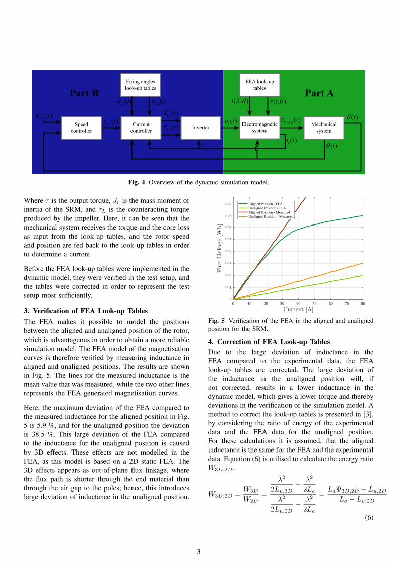
Fig. 4 Overview of the dynamic simulation model.

Where τ is the output torque, Jr is the mass moment ofinertia of the SRM, and τL is the counteracting torqueproduced by the impeller. Here, it can be seen that themechanical system receives the torque and the core lossas input from the look-up tables, and the rotor speedand position are fed back to the look-up tables in orderto determine a current.

Before the FEA look-up tables were implemented in thedynamic model, they were verified in the test setup, andthe tables were corrected in order to represent the testsetup most sufficiently.

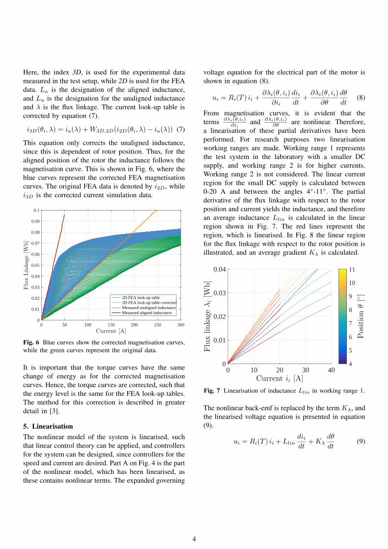
3. Verification of FEA Look-up TablesThe FEA makes it possible to model the positionsbetween the aligned and unaligned position of the rotor,which is advantageous in order to obtain a more reliablesimulation model. The FEA model of the magnetisationcurves is therefore verified by measuring inductance inaligned and unaligned positions. The results are shownin Fig. 5. The lines for the measured inductance is themean value that was measured, while the two other linesrepresents the FEA generated magnetisation curves.

Here, the maximum deviation of the FEA compared tothe measured inductance for the aligned position in Fig.5 is 5.9 %, and for the unaligned position the deviationis 38.5 %. This large deviation of the FEA comparedto the inductance for the unaligned position is causedby 3D effects. These effects are not modelled in theFEA, as this model is based on a 2D static FEA. The3D effects appears as out-of-plane flux linkage, wherethe flux path is shorter through the end material thanthrough the air gap to the poles; hence, this introduceslarge deviation of inductance in the unaligned position.

0 10 20 30 40 50 60 70 800

0.01

0.02

0.03

0.04

0.05

0.06

0.07

0.08 Aligned Position - FEAUnaligned Position - FEAAligned Position - MeasuredUnaligned Position - Measured

Fig. 5 Verification of the FEA in the aligned and unalignedposition for the SRM.

4. Correction of FEA Look-up TablesDue to the large deviation of inductance in theFEA compared to the experimental data, the FEAlook-up tables are corrected. The large deviation ofthe inductance in the unaligned position will, ifnot corrected, results in a lower inductance in thedynamic model, which gives a lower torque and therebydeviations in the verification of the simulation model. Amethod to correct the look-up tables is presented in [3],by considering the ratio of energy of the experimentaldata and the FEA data for the unaligned position.For these calculations it is assumed, that the alignedinductance is the same for the FEA and the experimentaldata. Equation (6) is utilised to calculate the energy ratioW3D,2D.

W3D,2D =W3D

W2D=

λ2

2Lu,3D− λ2

2Laλ2

2Lu,2D− λ2

2La

=LaΨ3D,2D − Lu,2D

La − Lu,2D

(6)

3

Here, the index 3D, is used for the experimental datameasured in the test setup, while 2D is used for the FEAdata. La is the designation of the aligned inductance,and Lu is the designation for the unaligned inductanceand λ is the flux linkage. The current look-up table iscorrected by equation (7).

i3D(θi, λ) = ia(λ) +W3D,2D(i2D(θi, λ)− ia(λ)) (7)

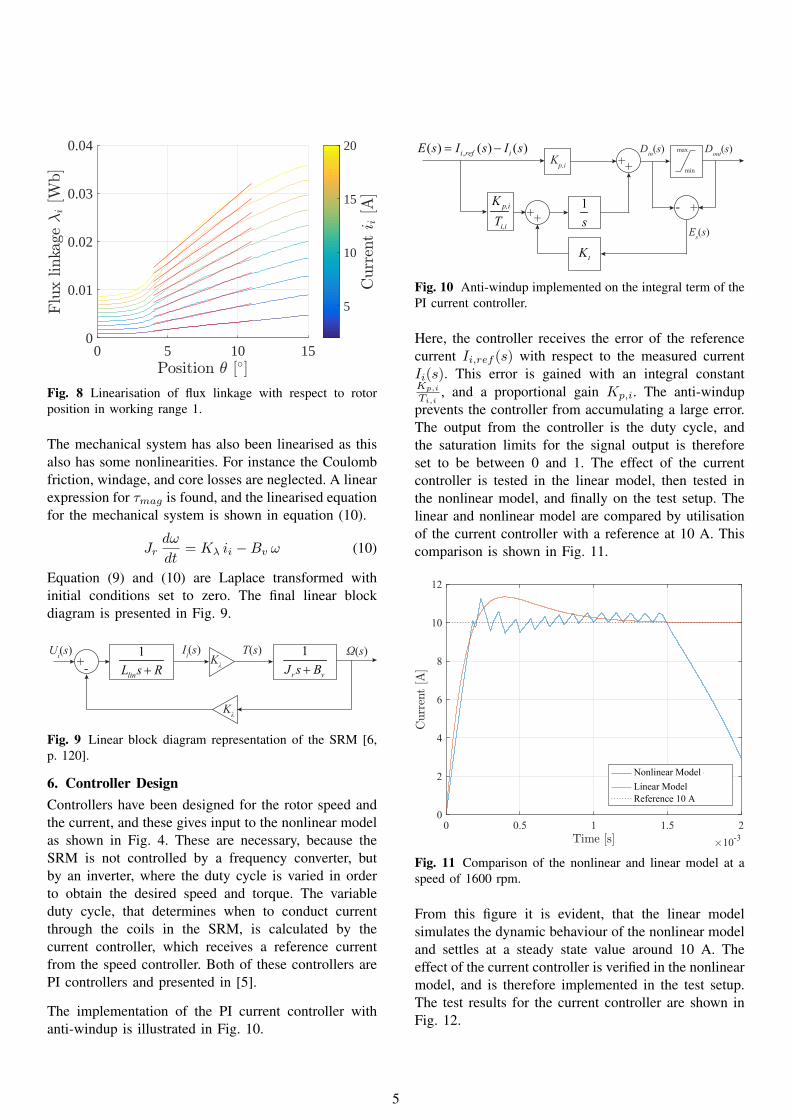
This equation only corrects the unaligned inductance,since this is dependent of rotor position. Thus, for thealigned position of the rotor the inductance follows themagnetisation curve. This is shown in Fig. 6, where theblue curves represent the corrected FEA magnetisationcurves. The original FEA data is denoted by i2D, whilei3D is the corrected current simulation data.

0 50 100 150 200 250 3000

0.01

0.02

0.03

0.04

0.05

0.06

0.07

0.08

0.09

0.1

2D FEA look-up table2D FEA look-up table correctedMeasured unaligned inductanceMeasured aligned inductance

Fig. 6 Blue curves show the corrected magnetisation curves,while the green curves represent the original data.

It is important that the torque curves have the samechange of energy as for the corrected magnetisationcurves. Hence, the torque curves are corrected, such thatthe energy level is the same for the FEA look-up tables.The method for this correction is described in greaterdetail in [3].

5. LinearisationThe nonlinear model of the system is linearised, suchthat linear control theory can be applied, and controllersfor the system can be designed, since controllers for thespeed and current are desired. Part A on Fig. 4 is the partof the nonlinear model, which has been linearised, asthese contains nonlinear terms. The expanded governing

voltage equation for the electrical part of the motor isshown in equation (8).

ui = Ri(T ) ii +∂λi(θ, ii)

∂ii

diidt

+∂λi(θ, ii)

∂θ

dθ

dt(8)

From magnetisation curves, it is evident that theterms ∂λi(θ,ii)

∂iiand ∂λi(θ,ii)

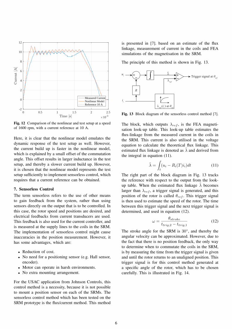
∂θ are nonlinear. Therefore,a linearisation of these partial derivatives have beenperformed. For research purposes two linearisationworking ranges are made. Working range 1 representsthe test system in the laboratory with a smaller DCsupply, and working range 2 is for higher currents.Working range 2 is not considered. The linear currentregion for the small DC supply is calculated between0-20 A and between the angles 4◦-11◦. The partialderivative of the flux linkage with respect to the rotorposition and current yields the inductance, and thereforean average inductance Llin is calculated in the linearregion shown in Fig. 7. The red lines represent theregion, which is linearised. In Fig. 8 the linear regionfor the flux linkage with respect to the rotor position isillustrated, and an average gradient Kλ is calculated.

0 10 20 30 400

0.01

0.02

0.03

0.04

4

5

6

7

8

9

10

11

Fig. 7 Linearisation of inductance Llin in working range 1.

The nonlinear back-emf is replaced by the term Kλ, andthe linearised voltage equation is presented in equation(9).

ui = Ri(T ) ii + Llindiidt

+Kλdθ

dt(9)

4

0 5 10 150

0.01

0.02

0.03

0.04

5

10

15

20

Fig. 8 Linearisation of flux linkage with respect to rotorposition in working range 1.

The mechanical system has also been linearised as thisalso has some nonlinearities. For instance the Coulombfriction, windage, and core losses are neglected. A linearexpression for τmag is found, and the linearised equationfor the mechanical system is shown in equation (10).

Jrdω

dt= Kλ ii −Bv ω (10)

Equation (9) and (10) are Laplace transformed withinitial conditions set to zero. The final linear blockdiagram is presented in Fig. 9.

+-1

linL s R+Kλ

T(s) 1

r vJ s B+Ω(s)

Kλ

Ui(s) Ii(s)

Fig. 9 Linear block diagram representation of the SRM [6,p. 120].

6. Controller DesignControllers have been designed for the rotor speed andthe current, and these gives input to the nonlinear modelas shown in Fig. 4. These are necessary, because theSRM is not controlled by a frequency converter, butby an inverter, where the duty cycle is varied in orderto obtain the desired speed and torque. The variableduty cycle, that determines when to conduct currentthrough the coils in the SRM, is calculated by thecurrent controller, which receives a reference currentfrom the speed controller. Both of these controllers arePI controllers and presented in [5].

The implementation of the PI current controller withanti-windup is illustrated in Fig. 10.

Kp,i

++1s

++Din(s) max

min

- +

Dout(s)

Es(s)

p,i

i,i

KT

,( ) ( ) ( )i ref iE s I s I s= −

tK

Fig. 10 Anti-windup implemented on the integral term of thePI current controller.

Here, the controller receives the error of the referencecurrent Ii,ref (s) with respect to the measured currentIi(s). This error is gained with an integral constantKp,i

Ti,i, and a proportional gain Kp,i. The anti-windup

prevents the controller from accumulating a large error.The output from the controller is the duty cycle, andthe saturation limits for the signal output is thereforeset to be between 0 and 1. The effect of the currentcontroller is tested in the linear model, then tested inthe nonlinear model, and finally on the test setup. Thelinear and nonlinear model are compared by utilisationof the current controller with a reference at 10 A. Thiscomparison is shown in Fig. 11.

0 0.5 1 1.5 210-3

0

2

4

6

8

10

12

Nonlinear Model (K =1)Linear ModelReference 10 A

Fig. 11 Comparison of the nonlinear and linear model at aspeed of 1600 rpm.

From this figure it is evident, that the linear modelsimulates the dynamic behaviour of the nonlinear modeland settles at a steady state value around 10 A. Theeffect of the current controller is verified in the nonlinearmodel, and is therefore implemented in the test setup.The test results for the current controller are shown inFig. 12.

5

0 0.5 1 1.5 2 2.5

10-3

-2

0

2

4

6

8

10

12

Measured CurrentNonlinear ModelReference 10 A

Fig. 12 Comparison of the nonlinear and test setup at a speedof 1600 rpm, with a current reference at 10 A.

Here, it is clear that the nonlinear model emulates thedynamic response of the test setup as well. However,the current build up is faster in the nonlinear model,which is explained by a small offset of the commutationangle. This offset results in larger inductance in the testsetup, and thereby a slower current build up. However,it is chosen that the nonlinear model represents the testsetup sufficiently to implement sensorless control, whichrequires that a current reference can be obtained.

7. Sensorless ControlThe term sensorless refers to the use of other meansto gain feedback from the system, rather than usingsensors directly on the output that is to be controlled. Inthis case, the rotor speed and positions are desired, andelectrical feedbacks from current transducers are used.This feedback is also used for the current controller, andis measured at the supply lines to the coils in the SRM.The implementation of sensorless control might causeinaccuracies in the position measurement. However, ithas some advantages, which are:

• Reduction of cost.• No need for a positioning sensor (e.g. Hall sensor,

encoder).• Motor can operate in harsh environments.• No extra mounting arrangement.

For the USAC application from Johnson Controls, thiscontrol method is a necessity, because it is not possibleto mount a position sensor on each of the SRMs. Thesensorless control method which has been tested on theSRM prototype is the flux/current method. This method

is presented in [7]. based on an estimate of the fluxlinkage, measurement of current in the coils and FEAsimulations of the magnetisation in the SRM.

The principle of this method is shown in Fig. 13.

+-ui

R

ii

λref (ii ) at θref

+-∫ Trigger signal at θref

λref

λ

Fig. 13 Block diagram of the sensorless control method [7].

The block, which outputs λref , is the FEA magneti-sation look-up table. This look-up table estimates theflux-linkage from the measured current in the coils inthe SRM. This current is also utilised in the voltageequation to calculate the theoretical flux linkage. Thisestimated flux linkage is denoted as λ̃ and derived fromthe integral in equation (11).

λ̃ =

∫t

(ui −Ri(T )ii)dt (11)

The right part of the block diagram in Fig. 13 tracksthe reference with respect to the output from the look-up table. When the estimated flux linkage λ̃ becomeslarger than λref , a trigger signal is generated, and thisposition of the rotor is called θref . This trigger signalis then used to estimate the speed of the rotor. The timebetween this trigger signal and the next trigger signal isdetermined, and used in equation (12).

ω =θstroke

ttrig,2 − ttrig,1(12)

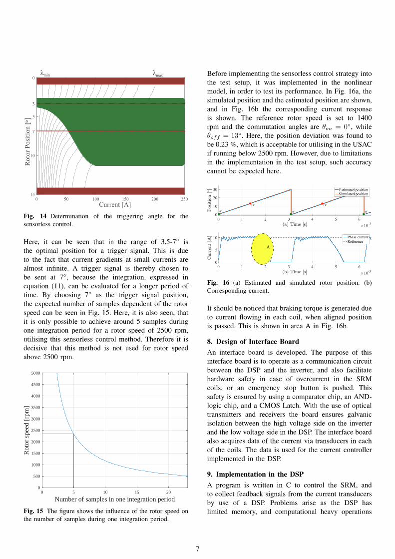
The stroke angle for the SRM is 30◦, and thereby theangular velocity can be approximated. However, due tothe fact that there is no position feedback, the only wayto determine when to commutate the coils in the SRM,is by measuring the time from the trigger signal is givenand until the rotor returns to an unaligned position. Thistrigger signal is for this control method generated ata specific angle of the rotor, which has to be chosencarefully. This is illustrated in Fig. 14.

6

0 50 100 150 200 250Current [A]

0

5

10

15

Rot

or P

ositi

on [ °

]

minλ maxλ

7

3

Fig. 14 Determination of the triggering angle for thesensorless control.

Here, it can be seen that in the range of 3.5-7◦ isthe optimal position for a trigger signal. This is dueto the fact that current gradients at small currents arealmost infinite. A trigger signal is thereby chosen tobe sent at 7◦, because the integration, expressed inequation (11), can be evaluated for a longer period oftime. By choosing 7◦ as the trigger signal position,the expected number of samples dependent of the rotorspeed can be seen in Fig. 15. Here, it is also seen, thatit is only possible to achieve around 5 samples duringone integration period for a rotor speed of 2500 rpm,utilising this sensorless control method. Therefore it isdecisive that this method is not used for rotor speedabove 2500 rpm.

0 5 10 15 20

Number of samples in one integration period

0

500

1000

1500

2000

2500

3000

3500

4000

4500

5000

Rot

or s

peed

[rp

m]

Fig. 15 The figure shows the influence of the rotor speed onthe number of samples during one integration period.

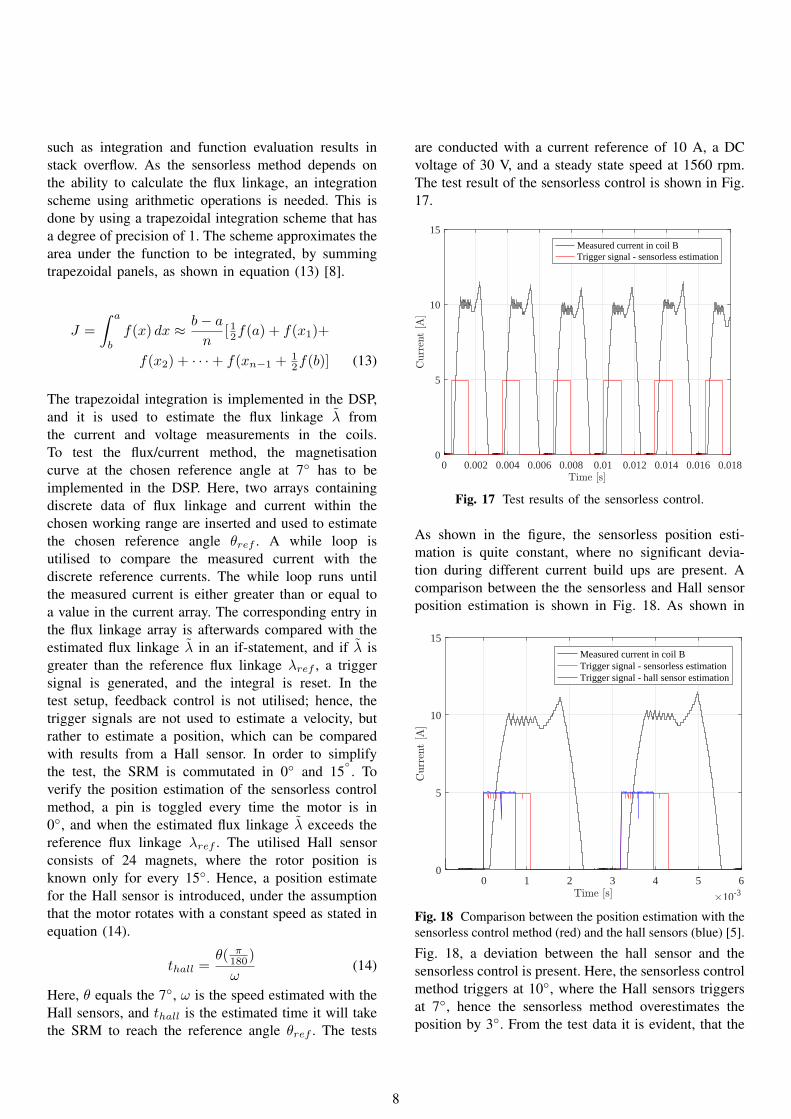
Before implementing the sensorless control strategy intothe test setup, it was implemented in the nonlinearmodel, in order to test its performance. In Fig. 16a, thesimulated position and the estimated position are shown,and in Fig. 16b the corresponding current responseis shown. The reference rotor speed is set to 1400rpm and the commutation angles are θon = 0◦, whileθoff = 13◦. Here, the position deviation was found tobe 0.23 %, which is acceptable for utilising in the USACif running below 2500 rpm. However, due to limitationsin the implementation in the test setup, such accuracycannot be expected here.

0 1 2 3 4 5 610-3

0

10

20

30Simulated positionEstimated position

0 1 2 3 4 5 610-3

0

5

10 Phase currentReference

13

0

13

0 0

A

Fig. 16 (a) Estimated and simulated rotor position. (b)Corresponding current.

It should be noticed that braking torque is generated dueto current flowing in each coil, when aligned positionis passed. This is shown in area A in Fig. 16b.

8. Design of Interface BoardAn interface board is developed. The purpose of thisinterface board is to operate as a communication circuitbetween the DSP and the inverter, and also facilitatehardware safety in case of overcurrent in the SRMcoils, or an emergency stop button is pushed. Thissafety is ensured by using a comparator chip, an AND-logic chip, and a CMOS Latch. With the use of opticaltransmitters and receivers the board ensures galvanicisolation between the high voltage side on the inverterand the low voltage side in the DSP. The interface boardalso acquires data of the current via transducers in eachof the coils. The data is used for the current controllerimplemented in the DSP.

9. Implementation in the DSPA program is written in C to control the SRM, andto collect feedback signals from the current transducersby use of a DSP. Problems arise as the DSP haslimited memory, and computational heavy operations

7

such as integration and function evaluation results instack overflow. As the sensorless method depends onthe ability to calculate the flux linkage, an integrationscheme using arithmetic operations is needed. This isdone by using a trapezoidal integration scheme that hasa degree of precision of 1. The scheme approximates thearea under the function to be integrated, by summingtrapezoidal panels, as shown in equation (13) [8].

J =

∫ a

b

f(x) dx ≈ b− an

[12f(a) + f(x1)+

f(x2) + · · ·+ f(xn−1 + 12f(b)] (13)

The trapezoidal integration is implemented in the DSP,and it is used to estimate the flux linkage λ̃ fromthe current and voltage measurements in the coils.To test the flux/current method, the magnetisationcurve at the chosen reference angle at 7◦ has to beimplemented in the DSP. Here, two arrays containingdiscrete data of flux linkage and current within thechosen working range are inserted and used to estimatethe chosen reference angle θref . A while loop isutilised to compare the measured current with thediscrete reference currents. The while loop runs untilthe measured current is either greater than or equal toa value in the current array. The corresponding entry inthe flux linkage array is afterwards compared with theestimated flux linkage λ̃ in an if-statement, and if λ̃ isgreater than the reference flux linkage λref , a triggersignal is generated, and the integral is reset. In thetest setup, feedback control is not utilised; hence, thetrigger signals are not used to estimate a velocity, butrather to estimate a position, which can be comparedwith results from a Hall sensor. In order to simplifythe test, the SRM is commutated in 0◦ and 15

◦. To

verify the position estimation of the sensorless controlmethod, a pin is toggled every time the motor is in0◦, and when the estimated flux linkage λ̃ exceeds thereference flux linkage λref . The utilised Hall sensorconsists of 24 magnets, where the rotor position isknown only for every 15◦. Hence, a position estimatefor the Hall sensor is introduced, under the assumptionthat the motor rotates with a constant speed as stated inequation (14).

thall =θ( π

180)

ω(14)

Here, θ equals the 7◦, ω is the speed estimated with theHall sensors, and thall is the estimated time it will takethe SRM to reach the reference angle θref . The tests

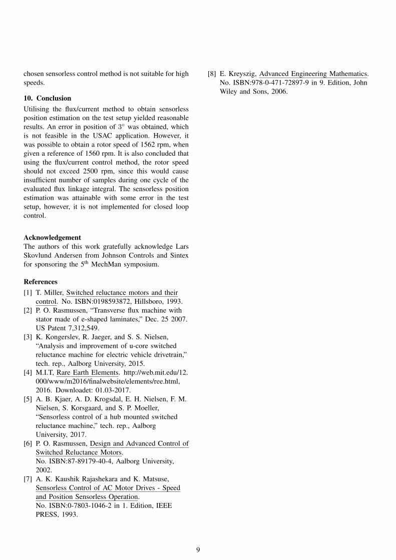
are conducted with a current reference of 10 A, a DCvoltage of 30 V, and a steady state speed at 1560 rpm.The test result of the sensorless control is shown in Fig.17.

0 0.002 0.004 0.006 0.008 0.01 0.012 0.014 0.016 0.0180

5

10

15

Measured current in coil BTrigger signal - sensorless estimation

Fig. 17 Test results of the sensorless control.

As shown in the figure, the sensorless position esti-mation is quite constant, where no significant devia-tion during different current build ups are present. Acomparison between the the sensorless and Hall sensorposition estimation is shown in Fig. 18. As shown in

0 1 2 3 4 5 6

10-3

0

5

10

15

Measured current in coil BTrigger signal - sensorless estimationTrigger signal - hall sensor estimation

Fig. 18 Comparison between the position estimation with thesensorless control method (red) and the hall sensors (blue) [5].

Fig. 18, a deviation between the hall sensor and thesensorless control is present. Here, the sensorless controlmethod triggers at 10◦, where the Hall sensors triggersat 7◦, hence the sensorless method overestimates theposition by 3◦. From the test data it is evident, that the

8

chosen sensorless control method is not suitable for highspeeds.

10. ConclusionUtilising the flux/current method to obtain sensorlessposition estimation on the test setup yielded reasonableresults. An error in position of 3◦ was obtained, whichis not feasible in the USAC application. However, itwas possible to obtain a rotor speed of 1562 rpm, whengiven a reference of 1560 rpm. It is also concluded thatusing the flux/current control method, the rotor speedshould not exceed 2500 rpm, since this would causeinsufficient number of samples during one cycle of theevaluated flux linkage integral. The sensorless positionestimation was attainable with some error in the testsetup, however, it is not implemented for closed loopcontrol.

AcknowledgementThe authors of this work gratefully acknowledge LarsSkovlund Andersen from Johnson Controls and Sintexfor sponsoring the 5th MechMan symposium.

References[1] T. Miller, Switched reluctance motors and their

control. No. ISBN:0198593872, Hillsboro, 1993.[2] P. O. Rasmussen, “Transverse flux machine with

stator made of e-shaped laminates,” Dec. 25 2007.US Patent 7,312,549.

[3] K. Kongerslev, R. Jaeger, and S. S. Nielsen,“Analysis and improvement of u-core switchedreluctance machine for electric vehicle drivetrain,”tech. rep., Aalborg University, 2015.

[4] M.I.T, Rare Earth Elements. http://web.mit.edu/12.000/www/m2016/finalwebsite/elements/ree.html,2016. Downloadet: 01.03-2017.

[5] A. B. Kjaer, A. D. Krogsdal, E. H. Nielsen, F. M.Nielsen, S. Korsgaard, and S. P. Moeller,“Sensorless control of a hub mounted switchedreluctance machine,” tech. rep., AalborgUniversity, 2017.

[6] P. O. Rasmussen, Design and Advanced Control ofSwitched Reluctance Motors.No. ISBN:87-89179-40-4, Aalborg University,2002.

[7] A. K. Kaushik Rajashekara and K. Matsuse,Sensorless Control of AC Motor Drives - Speedand Position Sensorless Operation.No. ISBN:0-7803-1046-2 in 1. Edition, IEEEPRESS, 1993.

[8] E. Kreyszig, Advanced Engineering Mathematics.No. ISBN:978-0-471-72897-9 in 9. Edition, JohnWiley and Sons, 2006.

9