Shear-induced fragmentation of Laponite suspensions

Thomas Gibaud∗,1 Catherine Barentin,2 Nicolas Taberlet,1 and Sebastien Manneville1, †

1Laboratoire de Physique, Universite de Lyon – Ecole Normale Superieure de Lyon – CNRS UMR 5672

46 allee d’Italie, 69364 Lyon cedex 07, France2Laboratoire de Physique de la Matiere Condensee et Nanostructures, Universite de Lyon – CNRS UMR 5586

43 Boulevard du 11 Novembre 1918, 69622 Villeurbanne cedex, France

(Dated: March 30, 2009)

Simultaneous rheological and velocity profile measurements are performed in a smooth Couettegeometry on Laponite suspensions seeded with glass microspheres and undergoing the shear-inducedsolid-to-fluid (or yielding) transition. Under these slippery boundary conditions, a rich temporalbehaviour is uncovered, in which shear localization is observed at short times, that rapidly givesway to a highly heterogeneous flow characterized by intermittent switching from plug-like flow tolinear velocity profiles. Such a temporal behaviour is linked to the fragmentation of the initiallysolid sample into blocks separated by fluidized regions. These solid pieces get progressively erodedover time scales ranging from a few minutes to several hours depending on the applied shear rateγ. The steady-state is characterized by a homogeneous flow with almost negligible wall slip. Thecharacteristic time scale for erosion is shown to diverge below some critical shear rate γ? and toscale as (γ − γ?)−n with n ' 2 above γ?. A tentative model for erosion is discussed together withopen questions raised by the present results.

PACS numbers: 83.60.La, 83.50.Rp, 83.60.Pq, 83.50.Lh

INTRODUCTION

Interest into the solid-to-fluid transition displayed by“soft glassy materials” (SGM) has risen tremendouslyin the past two decades not only because of its indus-trial importance but also due to its inherent theoreticalissues and experimental challenges. On the theoreticalside, the fact that this transition, also referred to asthe “jamming-unjamming” transition, can be triggeredeither by increasing the temperature, by lowering thesystem concentration, or by applying a strong enoughexternal load has led to propose a universal “jammingphase diagram” [1, 2]. Although this picture remains ap-pealing, it is clear that a complete understanding andmodelling of glassy-like phenomena involved in materi-als with microstructures as diverse as submicron hardspheres, micronsized grains, short-range attractive par-ticles, or highly charged platelets, are still out of reach[3]. Most recent experiments performed to investigatethe structure and the dynamics of SGM at rest have re-lied on single or multiple light scattering techniques andhave focused on ageing properties [4] or on the presenceof dynamical heterogeneities [5–7]. Together, ageing anddynamical heterogeneities call for a spatiotemporal mod-elling of SGM that is still lacking.

Even more difficult is the task of elucidating the flow

mechanisms in these out-of-equilibrium systems whensubmitted to some external shear. Rheology has long ap-peared as the only tool to probe the mechanical response

∗Present address: Brandeis University, Physics Department, 415

South Street, Waltham, MA 02453, USA

of SGM and the shear-induced solid-to-fluid transition,also called the “yielding transition.” In particular, theproblem of defining and measuring correctly the yield

stress σy, i.e. the critical shear stress below which thematerial behaves as a solid and above which it flows likea liquid, has focused a lot of attention [8]. The diffi-culties raised by the yield stress most often result fromthixotropic features due to the competition between age-ing and shear-induced “rejuvenation” of the sample [9].Thus estimating precisely σy involves applying or mea-suring very small shear rates over waiting times that canreach several hours.

Yield stress fluids and shear localization

Some authors have proposed to distinguish between a“static” yield stress σs

y , defined for the material at rest,that would be the analogue of a static friction coefficient,and a smaller “dynamic” yield stress σd

y , measured on theflowing material by decreasing the imposed stress, simi-lar to a dynamic friction coefficient [10]. Such a discrep-ancy linked to hysteresis effects also raises the questionof whether the yielding transition in SGM is continuous,i.e. the shear rate γ continuously increases from zerowhen the shear stress σ is increased above σy , or ratherdiscontinuous, i.e. γ jumps to some finite critical valueγc as soon as σ > σy.

Continuous models for the flow curve σ vs γ include theBingham and the Herschel-Bulkley models, which havebeen recognized to hold for many SGM [11, 12]. On theother hand, a discontinuous yielding transition questionsthe basic assumption of homogeneous flow that underliesany standard rheological measurement [10, 13]. Indeed,

2

if a shear rate γ < γc is applied, the flow is expected todisplay shear localization, i.e. the coexistence of a solid-like region where the local shear rate γloc vanishes and afluid-like region where γloc = γc.

The recent development of original experimental tools,such as active or passive microrheology [14, 15], lightscattering under shear, and time-resolved local velocime-try, that can go beyond standard rheology, has allowedone to address some of the above mentioned issues withrenewed interest. In particular, using direct visualiza-tion, nuclear magnetic resonance (NMR), particle imag-ing, or ultrasonic velocimetry, shear localization was ob-served on a large variety of SGM, ranging from emulsions[16–18] or colloidal suspensions [19–23] to wet granularmaterials [24, 25]. Still, in most of these experiments per-formed in Couette geometry, it remained unclear whethershear localization could be attributed to a truly non-zeroγc or to the stress inhomogeneity inherent to the concen-tric cylinder geometry. It is not until very recently thatshear localization has been also evidenced in the cone-and-plate geometry where stress heterogeneity is mini-mized, thus establishing firmly the relevance of discon-tinuous models [26].

Structure and rheology of Laponite suspensions

Within the last decade, among the huge variety ofSGM, Laponite, a synthetic clay of the hectorite typemade of heavily charged disc-shaped particles of diame-ter 25–30 nm, thickness 1 nm, and density 2.5 g.cm−3,has emerged as a good, albeit complicated, candidate toexplore the above issues. When dispersed into water at afew weight percents, typically 0.6–4 wt. %, and depend-ing on the ionic strength, Laponite suspensions evolvefrom a low-viscosity liquid to various solid-like “arrested”states. The sol–gel transition in Laponite has been inves-tigated mostly using light scattering [27–31]. The ageingproperties of Laponite have triggered lots of effort and de-bate about the exact nature of these nonergodic states,in particular, about whether the material is actually a“gel” or a (Wigner) “glass” [30, 32–38]. Moreover, dueto their out-of-equilibrium nature, Laponite suspensionswere used to test possible violations of the fluctuation-dissipation theorem (FDT) [39, 40]. Several recent mi-crorheology experiments tend to prove that the effectivetemperature cannot be distinguished from the bath tem-perature, so that the FDT remains valid [41, 42], butsuch results are still under debate [43].

The nonlinear rheology of Laponite suspensions hasalso been intensively studied with emphasis on thixotropyand ageing or rejuvenation under shear [27, 44–51]. Afew experiments have hinted to the presence of shear lo-calization in the vicinity of the yield stress in Laponitesamples [19, 52, 53], which provided support for discon-tinuous models of the yielding transition [10, 26]. How-

ever, to the best of our knowledge, the local velocity fieldof Laponite suspensions was measured only in a wide-gap(2 cm) Couette cell with a temporal resolution of about25 s per velocity profile using NMR velocimetry [52] andin a plate-plate geometry of gap 7 mm through dynamiclight scattering (DLS) [53]. The two corresponding pa-pers only showed a couple of velocity profiles, the for-mer raising the issue of strong geometry-induced stressheterogeneity and the latter reporting both wall slip andslow temporal oscillations of the velocity with the impor-tant limitation that DLS only provides point-like velocitymeasurements and necessitates to mechanically shift thecell in order to scan the whole gap. Therefore a system-atic time-resolved study of velocity profiles in shearedLaponite suspensions would certainly provide new in-sights into the flow mechanisms involved in yielding.

Summary of our previous and present work

In a previous work [54], we have explored for thefirst time the influence of boundary conditions on yield-ing in Laponite samples by simultaneous rheology andtime-resolved ultrasonic velocimetry. For the purpose ofmeasuring local velocity using ultrasound, a significant0.3 wt. % amount of hollow glass spheres of mean di-ameter 6 µm was added to our 3 wt. % Laponite sus-pensions. By comparing two experiments performed un-der similar imposed shear rates in smooth and rough(sand-blasted) Couette geometries on timescales of order5000 s, we unveiled a dramatic effect of surface rough-ness on the flow mechanism during yielding. Indeed,while the scenario observed with rough walls was con-sistent with a discontinuous transition characterized byshear localization in agreement with previous observa-tions on Laponite suspensions [19, 52, 53] and on otherSGM [16, 20, 22, 23, 26], slippery boundary conditionsin the smooth cell led to a thoroughly different picture.When wall slip was allowed, the sample was reported tobreak up into macroscopic solid pieces that are slowlyeroded by the surrounding fluidized material up to thepoint where the whole sample has become fluid.

The aim of the present paper is to provide a full dataset, more discussion, and a toy model of this originalyielding scenario triggered by slippery boundary condi-tions in Laponite suspensions seeded with microspheres.Our paper is organized as follows. Section describes thematerials and methods used to study the yielding transi-tion in Laponite. Results obtained in a smooth Couettecell on a 3 wt. % Laponite sample seeded with 1 wt. %microspheres are presented in Section for a large rangeof applied shear rates. Finally, Section provides a dis-cussion of the results, in particular about the possibleinfluence of the microsphere concentration, and an at-tempt to model the experimental observations.

3

EXPERIMENTAL

Sample preparation

Laponite powder (Rockwood, grade RD) is used as re-ceived and dispersed at 3 wt. % in ultrapure water withno added salt. The pH of the solution is approximately10. According to the most recent litterature [37, 38], sucha suspension (3 wt. % Laponite without salt) is supposedto fall into the Wigner glass region of the phase diagram.

In the present study, the Laponite suspensions are im-mediately seeded with hollow glass spheres of mean di-ameter 6 µm (Sphericel, Potters) at a weight fraction 0.3or 1 wt. %. As explained below in Section , these micro-spheres act as contrast agents for ultrasonic velocimetry.Most of current protocols used for Laponite preparationrecommend to filter the samples with a 0.4–0.8 µm meshsize after vigorous stirring for 15–30 min. Such filtra-tion is believed to break up Laponite clusters that mayform due to incomplete dissolution and may lead to erro-neous interpretations of the sample structure as “gel-like”from light scattering data [55]. Here, however, due to thepresence of the microspheres, subsequent filtration of thesamples is not possible.

Within 30 min of magnetic stirring, the dispersion be-comes homogeneous and very viscous but remains fluid.Due to the presence of the microspheres, the solution isslightly turbid, which will allow for direct visual inspec-tion of the sheared samples. The sample is then left torest at room temperature. After about two hours, thesample viscosity has increased by several orders of mag-nitude and the dispersion has clearly built up a yieldstress and solid-like properties since it is able to sustainits own weight. We let ageing proceed for at least twodays, i.e. for waiting times tw & 2 105 s. For such largetw, we expect the ageing dynamics to have slowed downso much that the influence of ageing can be neglectedon the timescales of typically one hour involved in thepresent experiments. In any case, as discussed below,the samples are pre-sheared before any experiments inorder to erase most of the sample history through shearrejuvenation.

Rheological protocol

Linear and nonlinear rheological properties are mea-sured using a stress-controlled rheometer (Bohlin C-VOR150, Malvern Instruments) in Mooney-Couette (concen-tric cylinder) geometry. Our cell is made out of Plexiglaswithout further treatment. The bob (inner cylinder) ofradius R1 = 24 mm is rotating and will be called the “ro-tor” in the following. It is terminated by a cone with anangle of 2.3◦. The stator, i.e. the fixed cup (outer cylin-der), has a radius R2 = 25 mm. The gap width of thisMooney-Couette geometry is thus e = R2 −R1 = 1 mm.

The curvature of our cell leads to a stress decrease ofabout 8 % from the rotor to the stator. The height of therotor is H = 30 mm. The standard deviation of heightprofiles of the cylindrical walls measured using atomicforce microscopy is typically 15 nm, which will be re-ferred to as “smooth.” The whole cell is immersed in awater tank of volume of about 1 L connected to a waterbath whose temperature is kept constant and equal to25±0.1◦C (see Fig. 1).

Before any measurement, the sample is pre-sheared for1 min at +1500 s−1 and for 1 min at -1500 s−1. Such aprotocol erases most of the sample history through shearrejuvenation and ensures that the strain of the sampleaccumulated during loading into the cell has no influence[44]. We then proceed with a standard oscillatory test at1 Hz in the linear regime for 2 min. This test allows usto make sure that the values of the viscoelastic moduliG′ ' 500 Pa and G′′ ' 25 Pa no longer change signifi-cantly at the beginning of the actual experiment. We alsochecked that this procedure leads to reproducible resultsover a few hours. Finally, at time t = 0, the experimentproceeds either with the standard (linear or nonlinear)rheological tests shown in Section or with combined rhe-ological and velocimetry measurements (see Section ).In the following, σ and γ denote the shear stress and theshear rate indicated by the rheometer. The rotor velocityv0 and γ are linked by:

v0 =R1(R1 + R2)

R21 + R2

2

γe , (1)

where the geometrical factor R1(R1 + R2)/(R21 + R2

2) ac-counts for the cell curvature [56]. In the presence of wallslip or heterogeneous flows, γ, the so-called “engineering”or “global” shear rate may strongly differ from the localshear rate which will be noted γloc or γ(r), where r is theradial distance from the rotor.

Ultrasonic velocimetry and optical imaging

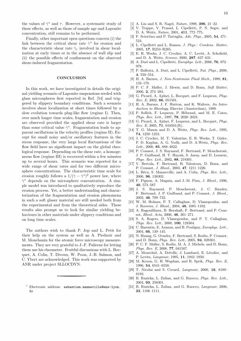
Our setup for combined rheology and local velocime-try is sketched in Fig. 1. The sample velocity field ismeasured using ultrasonic speckle velocimetry (USV) atabout 15 mm from the cell bottom. USV is a techniquethat allows one to access velocity profiles in Couette ge-ometry with a spatial resolution of 40 µm and a tempo-ral resolution of 0.02–2 s depending on the shear rate.It relies on the analysis of successive ultrasonic specklesignals that result from the interferences of the backscat-tered echoes of successive incident pulses of central fre-quency 36 MHz generated by a high-frequency piezo-polymer transducer (Panametrics PI50-2) connected toa broadband pulser-receiver (Panametrics 5900PR with200 MHz bandwidth). The speckle signals are sent to ahigh-speed digitizer (Acqiris DP235 with 500 MHz sam-pling frequency) and stored on a PC for post-processing

4

using a cross-correlation algorithm that yields the localdisplacement from one pulse to another as a function ofthe radial position r across the gap. One velocity profileis then obtained by averaging over typically 1000 suc-cessive cross-correlations. Full details about the USVtechnique may be found in Ref. [57].

The scattered signal is provided either by the materialmicrostructure itself or by seeding the fluid with “con-trast agents” with the constraint to remain in the sin-gle scattering regime. In the case of Laponite samples,which are transparent to ultrasound, we used the micro-spheres described above to produce ultrasonic echoes ina controlled way. The sound speed in our samples wasindependently measured to be c = 1495 ± 5 m.s−1 at25◦C.

The microspheres also lead to a slight turbidity whichallows for a direct visualization of the sheared samples.A simple CCD camera (Cohu 4192) is set in front of thewater tank and the Couette cell is lit from behind. Im-ages of the samples are recorded at a frame rate of 5 fpsand later synchronized with the velocity profile measure-ments as explained in our previous work [54]. In thispaper, we shall only show images typical of the variousstages of the experiment.

RESULTS

Conventional rheometry

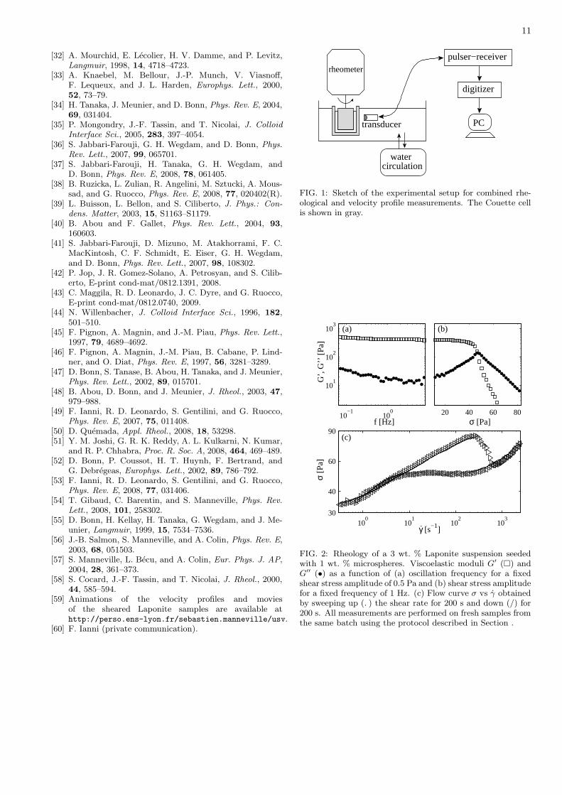
Standard rheological measurements performed on a3 wt. % Laponite suspension seeded with 1 wt. % mi-crospheres are shown in Fig. 2. The viscoelastic modulidisplayed in Fig. 2(a) and measured in the linear regimefor a shear stress amplitude of 5 Pa (which correspondsto a strain of at most 0.13 % over the accessible range offrequencies) are typical of an arrested (gel or glass) state.The elastic modulus G′ is always much larger than theloss modulus G′′ and only decays from 500 Pa to 400 Paover frequencies f = 0.07–8 Hz. G′′ also slowly decreasesfrom about 30 Pa to 15 Pa over this range of frequen-cies and shows no sign of downturn at low frequencies, afeature that is usually attributed to the presence of veryslow relaxation modes in SGM [12, 14].

Figure 2(b) shows the evolution of the viscoelasticmoduli in the nonlinear regime for shear stress ampli-tudes above 15 Pa at a fixed frequency of 1 Hz. Thesedata clearly point to a yield stress of 47 Pa, when de-fined as the shear stress amplitude σy for which G′(σy) =G′′(σy). This yield stress corresponds to a strain of 25 %.Above σy , G′ drops dramatically and rapidly becomesnegligible when compared to G′′. In other words, thesample becomes fluid above σy.

All these measurements are fully consistent with previ-ous data on Laponite suspensions [32, 44, 58]. Note thatthe addition of microspheres influences the ionic strength

of the suspension. The conductivity of a 1 % wt. suspen-sion of our glass microspheres in water was measured tobe about 100 µS.cm−1, which is roughly equivalent to asalt (NaCl) concentration of 0.8 10−3 mol.L−1. Increas-ing the microsphere concentration induces a noticeablestiffening of our samples: G′ increases by about 20 %when the microsphere concentration is increased from0.3 wt. % to 1 wt. % probably due to the change in ionicstrength [32].

As explained in the introduction, another way to probethe yielding transition using rheology is to perform non-linear measurements where a constant shear stress orshear rate is imposed. Since the flow curve is almostflat for small shear rates, it is usually more suitable towork under imposed shear rate. Figure 2(c) shows theflow curve obtained through a shear rate sweep from 0.3to 2500 s−1 within 200 s followed by the correspond-ing downward sweep at the same rate. The most ob-vious feature of this flow curve is the large hysteresisbetween upward and downward sweeps. This is typicalof thixotropic materials whose microstructure is slowlymodified by shear resulting in a time-dependent appar-ent viscosity η = σ/γ. The very same kind of hysteresiscycle was observed recently for similar shear rates in adrilling mud [22].

Following previous works [17, 22], we anticipate thatthe yield stress corresponds to the value of the shearstress on the plateau observed during the downwardsweep. This yields σy ' 51 Pa in satisfactory agree-ment with the previous estimate of 47 Pa, so that onehas σy = 49 ± 2 Pa. Finally, the shape of the flow curveat low shear rates (γ . 0.5 s−1) points to significantwall slip which is highly probable in our smooth geom-etry [17]. However, as we shall see below through time-resolved measurement of the local velocity, interpretingsuch a non-stationary flow curve is difficult due to com-plex temporal behaviours that take place over time scalesof about one hour.

Combined velocimetry and rheology

In this section, we present the combined rheologicaland velocity profile measurements performed under im-posed shear rate on a 3 wt. % Laponite sample seededwith 1 wt. % microspheres in a smooth Couette cell. Asrecalled in the introduction, our previous experiments[54] with a lower microsphere concentration of 0.3 wt. %showed that slippery boundary conditions may lead to arather complex scenario of slow fragmentation and ero-sion of the initially solid material. In paragraph , weshall explore the influence of the imposed shear rate onthis scenario for a given microsphere concentration of1 wt. % through experiments performed over typically5000 s. The influence of the microsphere concentrationwill be addressed in paragraph .

5

In paragraph below, we focus on the velocity profilesrecorded within the first few minutes after the inceptionof shear. We show that the flow may first seem com-patible with a simple shear localization picture of criticalshear rate γc ' 125 s−1. However, as explained later inparagraph , shear localization does not correspond to thestationary state reached by the system and the experi-ments have to be conducted over time scales of the orderof one hour to probe the actual long-time flow behaviour.

Early stage after shear start-up

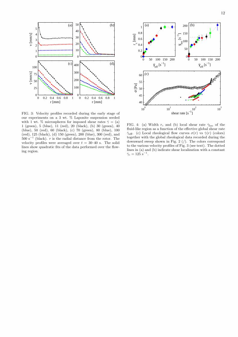
Figure 3 displays the velocity profiles v(r) averagedover t = 30–40 s after various shear rates γ ranging from1 to 500 s−1 are applied at time t = 0. The time win-dow for averaging the velocity profiles was chosen so thatfast initial transients due to flow inception have died out.Such transients last typically a few seconds, after whichthe dynamics becomes much slower and the velocity pro-files do not significantly change over 10 s. In the fol-lowing, we shall analyze these velocity profiles as if theycorresponded to steady measurements, keeping in mindthat, over time scales longer than a few minutes, a muchmore complex behaviour will emerge.

For γ . 10 s−1, total wall slip is observed and thematerial undergoes solid-body rotation. In this case, theshear rate effectively experienced by the material van-ishes, a feature that was already mentioned in Ref. [53].Above γ = 10 s−1, the velocity profiles are characterizedby a flowing zone close to the rotor that coexists withan “arrested” solid-like region where the local shear rateis zero. The size of the fluid-like region increases withthe imposed shear rate. For γ & 125 s−1, velocity pro-files are homogeneous and the whole sample is fluid onthe time window investigated here, i.e. after a few 10 s.These measurements are reminiscent of shear localizationas reported in various other SGM [16, 22, 23, 26].

Note that apparent wall slip remains significant at bothwalls as long as some “arrested” region is present. In-deed, for γ . 125 s−1, the velocity of the sample in theclose vicinity of the cell boundaries never reaches that ofthe walls, i.e. v(r = 0) < v0 at the rotor (where v0 isgiven by Eq. (1)) and v(r = e) > 0 at the stator. Wallslip becomes negligible only when a homogeneous flow isrecovered for γ & 125 s−1. In the following, in order tocompare our data with predictions and experiments ob-tained in the absence of wall slip, we shall focus on theeffective global shear rate γeff defined by [56]:

γeff =R2

1 + R22

R1(R1 + R2)

v(0) − v(e)

e, (2)

rather than on the applied shear rate γ.By using quadratic fits of the velocity profiles within

the fluid-like band, one may easily extract the width rc

of the flowing zone as well as the local shear rate γloc

averaged over this sheared region. Such an analysis ispresented as a function of the effective global shear rateγeff in Fig. 4(a) and (b). The error bars in Fig. 4(b) corre-spond to the standard deviation of the fitted local shearrate. It can be seen that the proportion of the shearedregion increases roughly linearly with γeff, consistentlywith the prediction of the simplest theoretical scenariofor shear localization [10, 16] and with recent experimen-tal findings on a colloidal gel [26]. Here, Fig. 4(a) clearlypoints to a critical shear rate γc ' 125 s−1.

Yet, Fig. 4(b) contradicts such a simple shear local-ization scenario. Indeed, it is clearly seen that the localshear rate γloc is not constant and equal to γc. It ratherincreases sharply from γloc ' 60 s−1 to 125 s−1 as γ isincreased. This is confirmed by looking at the “local”flow curves displayed in Fig. 4(c) and showing the localshear stress σ(r) plotted against the local shear rate γ(r).σ(r) is computed from the global shear stress σ measuredby the rheometer simultaneously to the velocity profilesusing [56]:

σ(r) =2R2

1R22

(R21 + R2

2)r2

σ , (3)

where the proportionality factor accounts for the Cou-ette geometry. The local shear rate γ(r) = −r ∂

∂r

(vr

)

is simply estimated from the derivative of the quadraticfits of the velocity profiles of Fig. 3. The resulting localflow curves σ(r) vs γ(r) are compared to the downwardsweep of Fig. 2(c) in Fig. 4(c). For the highest shearrates, the local data collapse rather well on the globalflow curve. This indicates that for γ & 200 s−1, the ma-terial becomes fully fluid-like almost instantly and thatno time-dependent phenomena further occur. For smallershear rates, the local flow curves reveal two interestingfeatures: (i) the existence of a “forbidden” range of localshear rates since γ(r) . 60 s−1 is never observed and(ii) the relevance of time-dependent, history-dependent,or metastable phenomena since the local shear stress fort = 30–40 s is significantly smaller than the shear stressrecorded during the downward sweep of Fig. 2(c). Fi-nally, for shear-localized velocity profiles, γ(r) covers therange 60–125 s−1.

In the next paragraph, we shall see that shear local-ization as revealed in Fig. 3 is only transient so that thenon-standard scenario shown in Fig. 4(b) and (c) is notso surprising. In any case, it is important to stress thefact that, if the velocity measurements had been stoppedafter a few minutes, shear localization could have beenwrongly interpreted as the steady-state for yielding inthis SGM.

Long-time flow behaviour

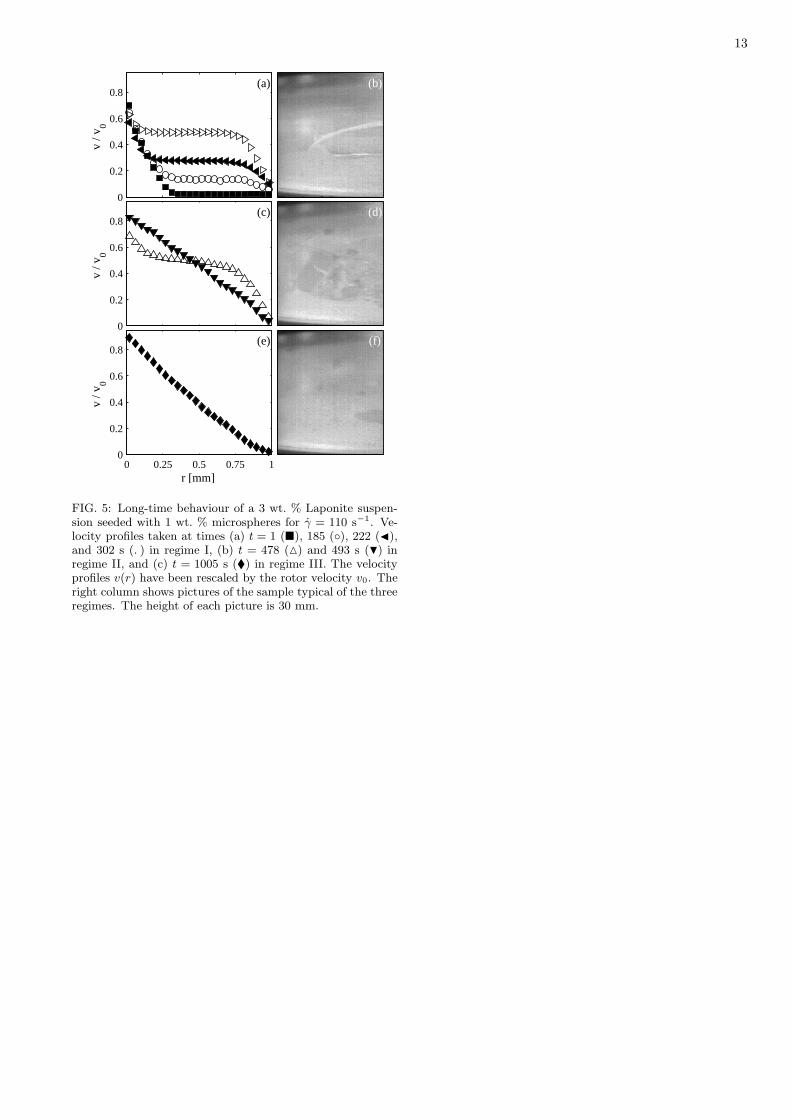
As shown in Fig. 5, the long-time behaviour of oursheared samples is not shear localization. A complex

6

spatio-temporal scenario rather develops on time scalesranging from a few minutes to several hours dependingon the applied shear rate. As in Ref. [54], we propose todistinguish three different regimes in the temporal evo-lution of the flow.

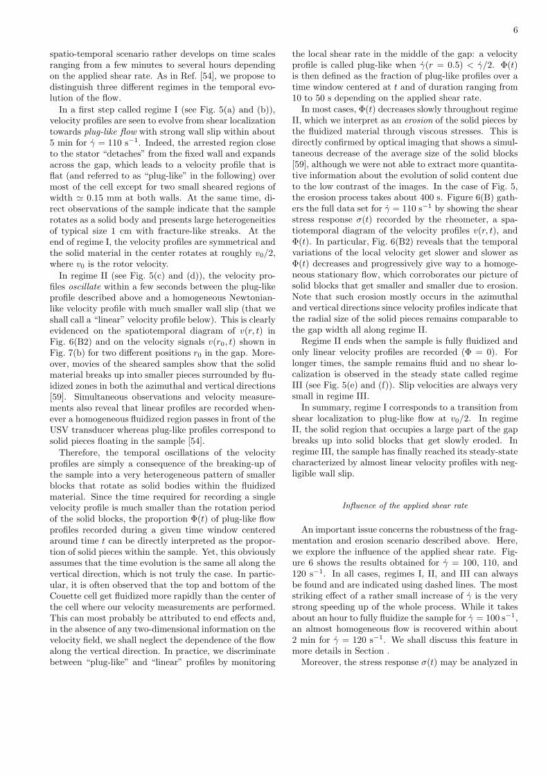
In a first step called regime I (see Fig. 5(a) and (b)),velocity profiles are seen to evolve from shear localizationtowards plug-like flow with strong wall slip within about5 min for γ = 110 s−1. Indeed, the arrested region closeto the stator “detaches” from the fixed wall and expandsacross the gap, which leads to a velocity profile that isflat (and referred to as “plug-like” in the following) overmost of the cell except for two small sheared regions ofwidth ' 0.15 mm at both walls. At the same time, di-rect observations of the sample indicate that the samplerotates as a solid body and presents large heterogeneitiesof typical size 1 cm with fracture-like streaks. At theend of regime I, the velocity profiles are symmetrical andthe solid material in the center rotates at roughly v0/2,where v0 is the rotor velocity.

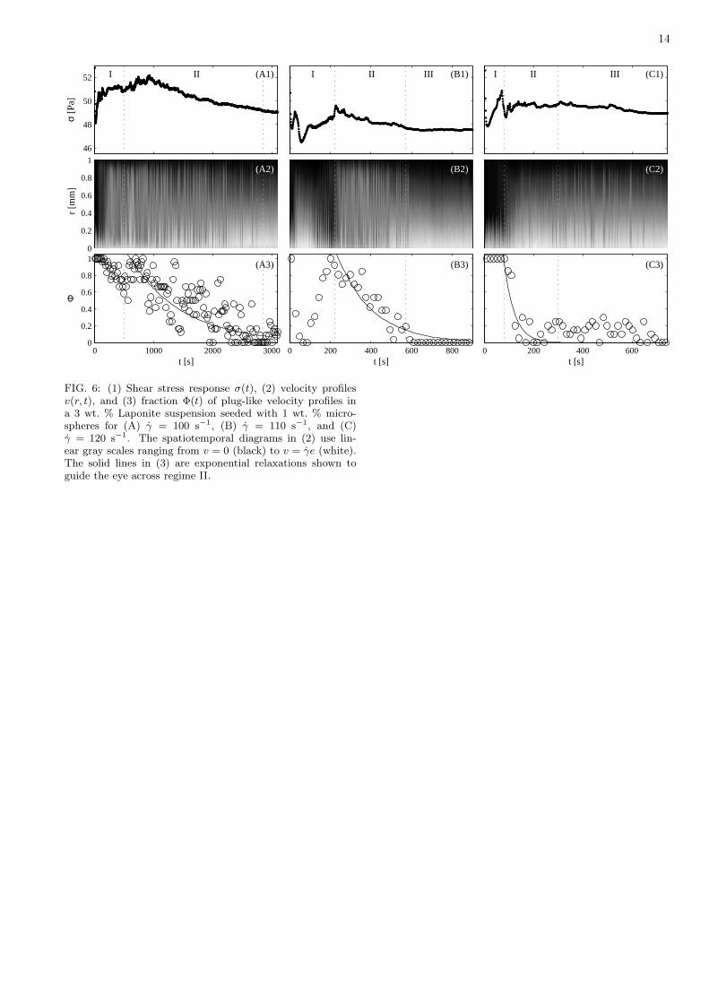
In regime II (see Fig. 5(c) and (d)), the velocity pro-files oscillate within a few seconds between the plug-likeprofile described above and a homogeneous Newtonian-like velocity profile with much smaller wall slip (that weshall call a “linear” velocity profile below). This is clearlyevidenced on the spatiotemporal diagram of v(r, t) inFig. 6(B2) and on the velocity signals v(r0, t) shown inFig. 7(b) for two different positions r0 in the gap. More-over, movies of the sheared samples show that the solidmaterial breaks up into smaller pieces surrounded by flu-idized zones in both the azimuthal and vertical directions[59]. Simultaneous observations and velocity measure-ments also reveal that linear profiles are recorded when-ever a homogeneous fluidized region passes in front of theUSV transducer whereas plug-like profiles correspond tosolid pieces floating in the sample [54].

Therefore, the temporal oscillations of the velocityprofiles are simply a consequence of the breaking-up ofthe sample into a very heterogeneous pattern of smallerblocks that rotate as solid bodies within the fluidizedmaterial. Since the time required for recording a singlevelocity profile is much smaller than the rotation periodof the solid blocks, the proportion Φ(t) of plug-like flowprofiles recorded during a given time window centeredaround time t can be directly interpreted as the propor-tion of solid pieces within the sample. Yet, this obviouslyassumes that the time evolution is the same all along thevertical direction, which is not truly the case. In partic-ular, it is often observed that the top and bottom of theCouette cell get fluidized more rapidly than the center ofthe cell where our velocity measurements are performed.This can most probably be attributed to end effects and,in the absence of any two-dimensional information on thevelocity field, we shall neglect the dependence of the flowalong the vertical direction. In practice, we discriminatebetween “plug-like” and “linear” profiles by monitoring

the local shear rate in the middle of the gap: a velocityprofile is called plug-like when γ(r = 0.5) < γ/2. Φ(t)is then defined as the fraction of plug-like profiles over atime window centered at t and of duration ranging from10 to 50 s depending on the applied shear rate.

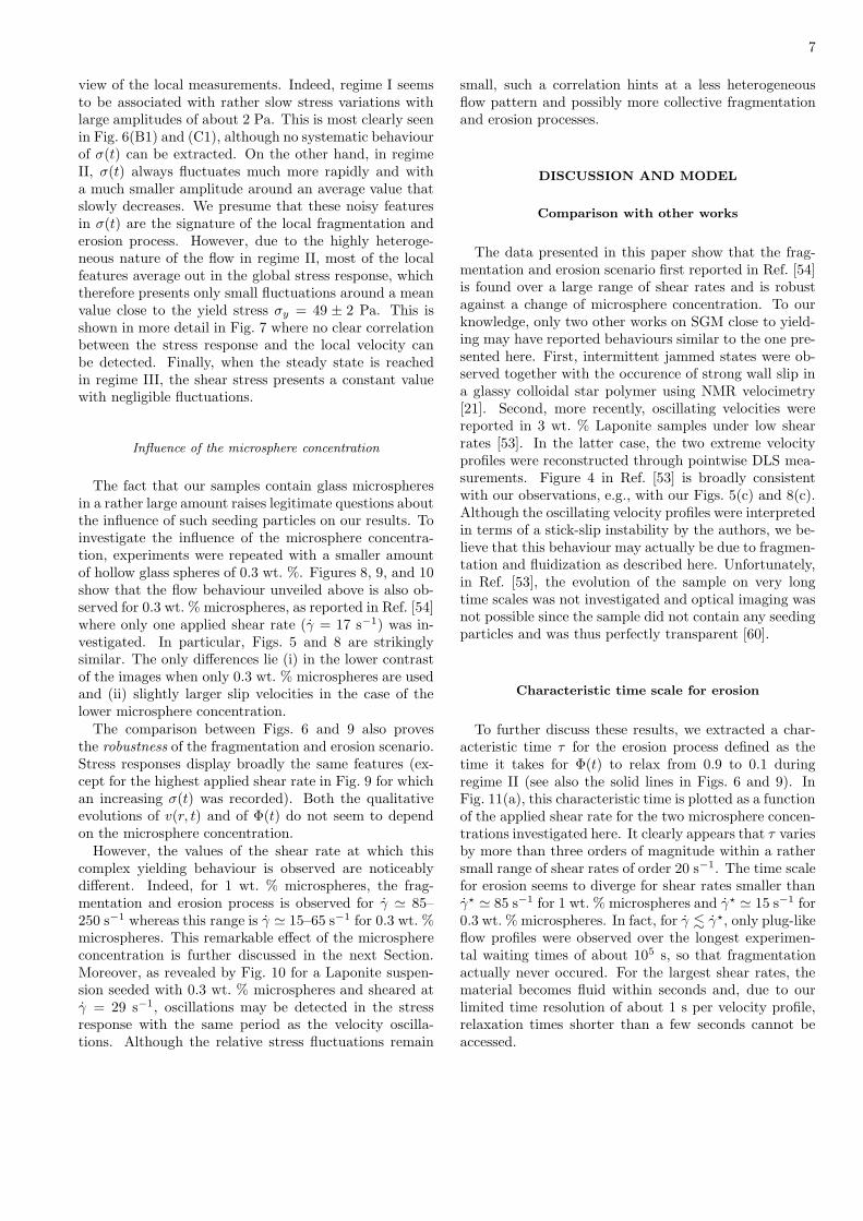
In most cases, Φ(t) decreases slowly throughout regimeII, which we interpret as an erosion of the solid pieces bythe fluidized material through viscous stresses. This isdirectly confirmed by optical imaging that shows a simul-taneous decrease of the average size of the solid blocks[59], although we were not able to extract more quantita-tive information about the evolution of solid content dueto the low contrast of the images. In the case of Fig. 5,the erosion process takes about 400 s. Figure 6(B) gath-ers the full data set for γ = 110 s−1 by showing the shearstress response σ(t) recorded by the rheometer, a spa-tiotemporal diagram of the velocity profiles v(r, t), andΦ(t). In particular, Fig. 6(B2) reveals that the temporalvariations of the local velocity get slower and slower asΦ(t) decreases and progressively give way to a homoge-neous stationary flow, which corroborates our picture ofsolid blocks that get smaller and smaller due to erosion.Note that such erosion mostly occurs in the azimuthaland vertical directions since velocity profiles indicate thatthe radial size of the solid pieces remains comparable tothe gap width all along regime II.

Regime II ends when the sample is fully fluidized andonly linear velocity profiles are recorded (Φ = 0). Forlonger times, the sample remains fluid and no shear lo-calization is observed in the steady state called regimeIII (see Fig. 5(e) and (f)). Slip velocities are always verysmall in regime III.

In summary, regime I corresponds to a transition fromshear localization to plug-like flow at v0/2. In regimeII, the solid region that occupies a large part of the gapbreaks up into solid blocks that get slowly eroded. Inregime III, the sample has finally reached its steady-statecharacterized by almost linear velocity profiles with neg-ligible wall slip.

Influence of the applied shear rate

An important issue concerns the robustness of the frag-mentation and erosion scenario described above. Here,we explore the influence of the applied shear rate. Fig-ure 6 shows the results obtained for γ = 100, 110, and120 s−1. In all cases, regimes I, II, and III can alwaysbe found and are indicated using dashed lines. The moststriking effect of a rather small increase of γ is the verystrong speeding up of the whole process. While it takesabout an hour to fully fluidize the sample for γ = 100 s−1,an almost homogeneous flow is recovered within about2 min for γ = 120 s−1. We shall discuss this feature inmore details in Section .

Moreover, the stress response σ(t) may be analyzed in

7

view of the local measurements. Indeed, regime I seemsto be associated with rather slow stress variations withlarge amplitudes of about 2 Pa. This is most clearly seenin Fig. 6(B1) and (C1), although no systematic behaviourof σ(t) can be extracted. On the other hand, in regimeII, σ(t) always fluctuates much more rapidly and witha much smaller amplitude around an average value thatslowly decreases. We presume that these noisy featuresin σ(t) are the signature of the local fragmentation anderosion process. However, due to the highly heteroge-neous nature of the flow in regime II, most of the localfeatures average out in the global stress response, whichtherefore presents only small fluctuations around a meanvalue close to the yield stress σy = 49 ± 2 Pa. This isshown in more detail in Fig. 7 where no clear correlationbetween the stress response and the local velocity canbe detected. Finally, when the steady state is reachedin regime III, the shear stress presents a constant valuewith negligible fluctuations.

Influence of the microsphere concentration

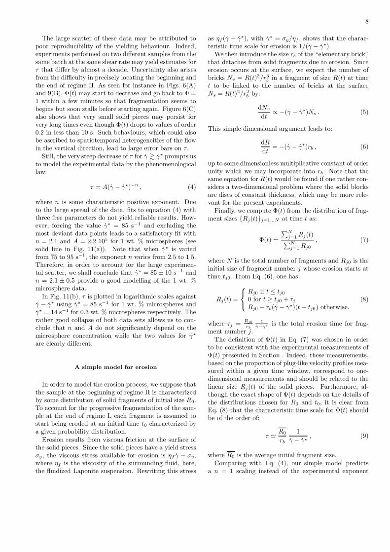
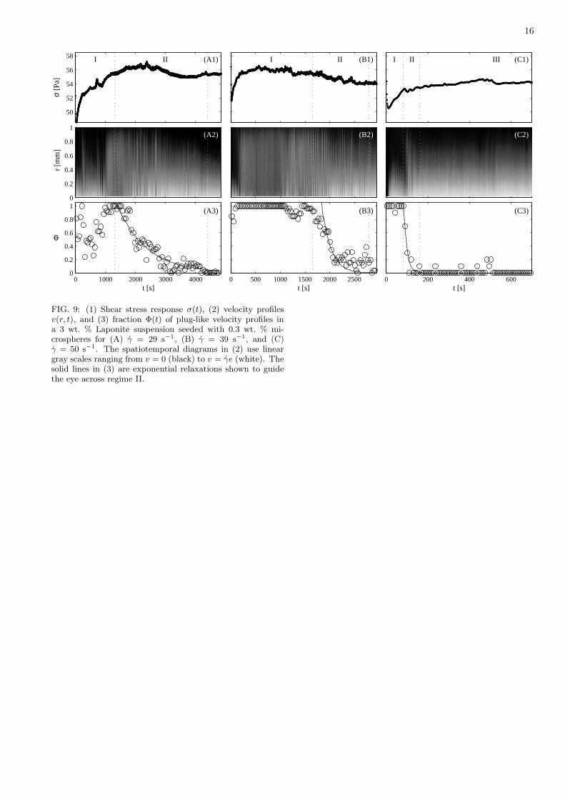
The fact that our samples contain glass microspheresin a rather large amount raises legitimate questions aboutthe influence of such seeding particles on our results. Toinvestigate the influence of the microsphere concentra-tion, experiments were repeated with a smaller amountof hollow glass spheres of 0.3 wt. %. Figures 8, 9, and 10show that the flow behaviour unveiled above is also ob-served for 0.3 wt. % microspheres, as reported in Ref. [54]where only one applied shear rate (γ = 17 s−1) was in-vestigated. In particular, Figs. 5 and 8 are strikinglysimilar. The only differences lie (i) in the lower contrastof the images when only 0.3 wt. % microspheres are usedand (ii) slightly larger slip velocities in the case of thelower microsphere concentration.

The comparison between Figs. 6 and 9 also provesthe robustness of the fragmentation and erosion scenario.Stress responses display broadly the same features (ex-cept for the highest applied shear rate in Fig. 9 for whichan increasing σ(t) was recorded). Both the qualitativeevolutions of v(r, t) and of Φ(t) do not seem to dependon the microsphere concentration.

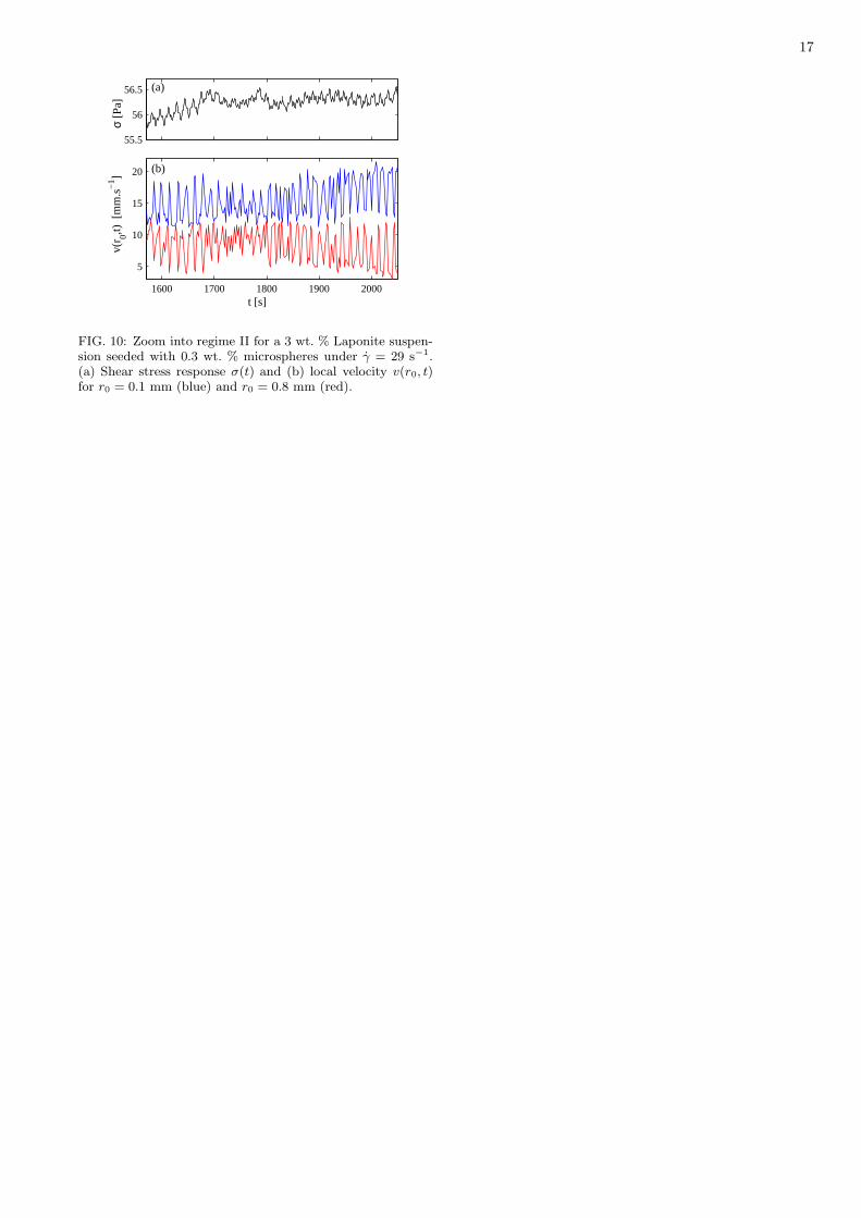
However, the values of the shear rate at which thiscomplex yielding behaviour is observed are noticeablydifferent. Indeed, for 1 wt. % microspheres, the frag-mentation and erosion process is observed for γ ' 85–250 s−1 whereas this range is γ ' 15–65 s−1 for 0.3 wt. %microspheres. This remarkable effect of the microsphereconcentration is further discussed in the next Section.Moreover, as revealed by Fig. 10 for a Laponite suspen-sion seeded with 0.3 wt. % microspheres and sheared atγ = 29 s−1, oscillations may be detected in the stressresponse with the same period as the velocity oscilla-tions. Although the relative stress fluctuations remain

small, such a correlation hints at a less heterogeneousflow pattern and possibly more collective fragmentationand erosion processes.

DISCUSSION AND MODEL

Comparison with other works

The data presented in this paper show that the frag-mentation and erosion scenario first reported in Ref. [54]is found over a large range of shear rates and is robustagainst a change of microsphere concentration. To ourknowledge, only two other works on SGM close to yield-ing may have reported behaviours similar to the one pre-sented here. First, intermittent jammed states were ob-served together with the occurence of strong wall slip ina glassy colloidal star polymer using NMR velocimetry[21]. Second, more recently, oscillating velocities werereported in 3 wt. % Laponite samples under low shearrates [53]. In the latter case, the two extreme velocityprofiles were reconstructed through pointwise DLS mea-surements. Figure 4 in Ref. [53] is broadly consistentwith our observations, e.g., with our Figs. 5(c) and 8(c).Although the oscillating velocity profiles were interpretedin terms of a stick-slip instability by the authors, we be-lieve that this behaviour may actually be due to fragmen-tation and fluidization as described here. Unfortunately,in Ref. [53], the evolution of the sample on very longtime scales was not investigated and optical imaging wasnot possible since the sample did not contain any seedingparticles and was thus perfectly transparent [60].

Characteristic time scale for erosion

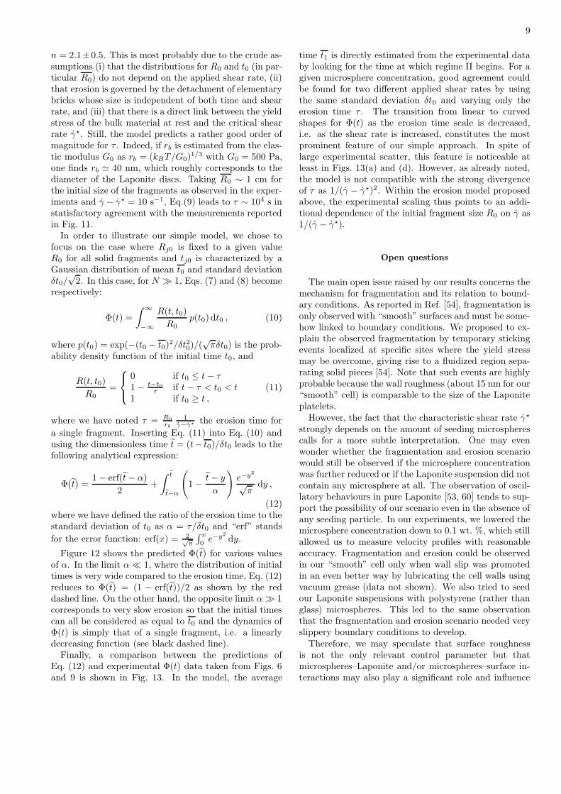
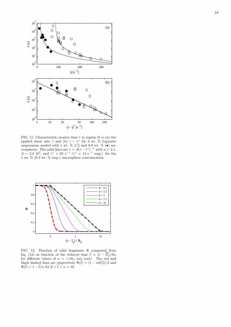
To further discuss these results, we extracted a char-acteristic time τ for the erosion process defined as thetime it takes for Φ(t) to relax from 0.9 to 0.1 duringregime II (see also the solid lines in Figs. 6 and 9). InFig. 11(a), this characteristic time is plotted as a functionof the applied shear rate for the two microsphere concen-trations investigated here. It clearly appears that τ variesby more than three orders of magnitude within a rathersmall range of shear rates of order 20 s−1. The time scalefor erosion seems to diverge for shear rates smaller thanγ? ' 85 s−1 for 1 wt. % microspheres and γ? ' 15 s−1 for0.3 wt. % microspheres. In fact, for γ . γ?, only plug-likeflow profiles were observed over the longest experimen-tal waiting times of about 105 s, so that fragmentationactually never occured. For the largest shear rates, thematerial becomes fluid within seconds and, due to ourlimited time resolution of about 1 s per velocity profile,relaxation times shorter than a few seconds cannot beaccessed.

8

The large scatter of these data may be attributed topoor reproducibility of the yielding behaviour. Indeed,experiments performed on two different samples from thesame batch at the same shear rate may yield estimates forτ that differ by almost a decade. Uncertainty also arisesfrom the difficulty in precisely locating the beginning andthe end of regime II. As seen for instance in Figs. 6(A)and 9(B), Φ(t) may start to decrease and go back to Φ =1 within a few minutes so that fragmentation seems tobegins but soon stalls before starting again. Figure 6(C)also shows that very small solid pieces may persist forvery long times even though Φ(t) drops to values of order0.2 in less than 10 s. Such behaviours, which could alsobe ascribed to spatiotemporal heterogeneities of the flowin the vertical direction, lead to large error bars on τ .

Still, the very steep decrease of τ for γ & γ? prompts usto model the experimental data by the phenomenologicallaw:

τ = A(γ − γ?)−n , (4)

where n is some characteristic positive exponent. Dueto the large spread of the data, fits to equation (4) withthree free parameters do not yield reliable results. How-ever, forcing the value γ? = 85 s−1 and excluding themost deviant data points leads to a satisfactory fit withn = 2.1 and A = 2.2 105 for 1 wt. % microspheres (seesolid line in Fig. 11(a)). Note that when γ? is variedfrom 75 to 95 s−1, the exponent n varies from 2.5 to 1.5.Therefore, in order to account for the large experimen-tal scatter, we shall conclude that γ? = 85 ± 10 s−1 andn = 2.1 ± 0.5 provide a good modelling of the 1 wt. %microsphere data.

In Fig. 11(b), τ is plotted in logarithmic scales againstγ − γ? using γ? = 85 s−1 for 1 wt. % microspheres andγ? = 14 s−1 for 0.3 wt. % microspheres respectively. Therather good collapse of both data sets allows us to con-clude that n and A do not significantly depend on themicrosphere concentration while the two values for γ?

are clearly different.

A simple model for erosion

In order to model the erosion process, we suppose thatthe sample at the beginning of regime II is characterizedby some distribution of solid fragments of initial size R0.To account for the progressive fragmentation of the sam-ple at the end of regime I, each fragment is assumed tostart being eroded at an initial time t0 characterized bya given probability distribution.

Erosion results from viscous friction at the surface ofthe solid pieces. Since the solid pieces have a yield stressσy, the viscous stress available for erosion is ηf γ − σy,where ηf is the viscosity of the surrounding fluid, here,the fluidized Laponite suspension. Rewriting this stress

as ηf (γ − γ?), with γ? = σy/ηf , shows that the charac-teristic time scale for erosion is 1/(γ − γ?).

We then introduce the size rb of the “elementary brick”that detaches from solid fragments due to erosion. Sinceerosion occurs at the surface, we expect the number ofbricks Nv = R(t)3/r3

b in a fragment of size R(t) at timet to be linked to the number of bricks at the surfaceNs = R(t)2/r2

b by:

dNv

dt∝ −(γ − γ?)Ns . (5)

This simple dimensional argument leads to:

dR

dt= −(γ − γ?)rb , (6)

up to some dimensionless multiplicative constant of orderunity which we may incorporate into rb. Note that thesame equation for R(t) would be found if one rather con-siders a two-dimensional problem where the solid blocksare discs of constant thickness, which may be more rele-vant for the present experiments.

Finally, we compute Φ(t) from the distribution of frag-ment sizes {Rj(t)}j=1...N at time t as:

Φ(t) =

∑Nj=1 Rj(t)∑N

j=1 Rj0

, (7)

where N is the total number of fragments and Rj0 is theinitial size of fragment number j whose erosion starts attime tj0. From Eq. (6), one has:

Rj(t) =

Rj0 if t ≤ tj00 for t ≥ tj0 + τj

Rj0 − rb(γ − γ?)(t − tj0) otherwise.(8)

where τj =Rj0

rb

1γ−γ? is the total erosion time for frag-

ment number j.The definition of Φ(t) in Eq. (7) was chosen in order

to be consistent with the experimental measurements ofΦ(t) presented in Section . Indeed, these measurements,based on the proportion of plug-like velocity profiles mea-sured within a given time window, correspond to one-dimensional measurements and should be related to thelinear size Rj(t) of the solid pieces. Furthermore, al-though the exact shape of Φ(t) depends on the details ofthe distributions chosen for R0 and t0, it is clear fromEq. (8) that the characteristic time scale for Φ(t) shouldbe of the order of:

τ ' R0

rb

1

γ − γ?, (9)

where R0 is the average initial fragment size.Comparing with Eq. (4), our simple model predicts

a n = 1 scaling instead of the experimental exponent

9

n = 2.1±0.5. This is most probably due to the crude as-sumptions (i) that the distributions for R0 and t0 (in par-ticular R0) do not depend on the applied shear rate, (ii)that erosion is governed by the detachment of elementarybricks whose size is independent of both time and shearrate, and (iii) that there is a direct link between the yieldstress of the bulk material at rest and the critical shearrate γ?. Still, the model predicts a rather good order ofmagnitude for τ . Indeed, if rb is estimated from the elas-tic modulus G0 as rb = (kBT/G0)

1/3 with G0 = 500 Pa,one finds rb ' 40 nm, which roughly corresponds to thediameter of the Laponite discs. Taking R0 ∼ 1 cm forthe initial size of the fragments as observed in the exper-iments and γ − γ? = 10 s−1, Eq.(9) leads to τ ∼ 104 s instatisfactory agreement with the measurements reportedin Fig. 11.

In order to illustrate our simple model, we chose tofocus on the case where Rj0 is fixed to a given valueR0 for all solid fragments and tj0 is characterized by aGaussian distribution of mean t0 and standard deviationδt0/

√2. In this case, for N � 1, Eqs. (7) and (8) become

respectively:

Φ(t) =

∫ ∞

−∞

R(t, t0)

R0

p(t0) dt0 , (10)

where p(t0) = exp(−(t0 − t0)2/δt20)/(

√πδt0) is the prob-

ability density function of the initial time t0, and

R(t, t0)

R0

=

0 if t0 ≤ t − τ1 − t−t0

τ if t − τ < t0 < t1 if t0 ≥ t ,

(11)

where we have noted τ = R0

rb

1γ−γ? the erosion time for

a single fragment. Inserting Eq. (11) into Eq. (10) andusing the dimensionless time t = (t− t0)/δt0 leads to thefollowing analytical expression:

Φ(t) =1 − erf(t − α)

2+

∫ et

et−α

(1 − t − y

α

)e−y2

√π

dy ,

(12)where we have defined the ratio of the erosion time to thestandard deviation of t0 as α = τ/δt0 and “erf” stands

for the error function: erf(x) = 2√π

∫ x

0e−y2

dy.

Figure 12 shows the predicted Φ(t) for various valuesof α. In the limit α � 1, where the distribution of initialtimes is very wide compared to the erosion time, Eq. (12)reduces to Φ(t) = (1 − erf(t))/2 as shown by the reddashed line. On the other hand, the opposite limit α � 1corresponds to very slow erosion so that the initial timescan all be considered as equal to t0 and the dynamics ofΦ(t) is simply that of a single fragment, i.e. a linearlydecreasing function (see black dashed line).

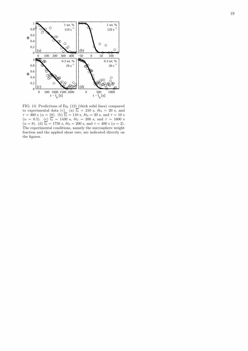
Finally, a comparison between the predictions ofEq. (12) and experimental Φ(t) data taken from Figs. 6and 9 is shown in Fig. 13. In the model, the average

time t1 is directly estimated from the experimental databy looking for the time at which regime II begins. For agiven microsphere concentration, good agreement couldbe found for two different applied shear rates by usingthe same standard deviation δt0 and varying only theerosion time τ . The transition from linear to curvedshapes for Φ(t) as the erosion time scale is decreased,i.e. as the shear rate is increased, constitutes the mostprominent feature of our simple approach. In spite oflarge experimental scatter, this feature is noticeable atleast in Figs. 13(a) and (d). However, as already noted,the model is not compatible with the strong divergenceof τ as 1/(γ − γ?)2. Within the erosion model proposedabove, the experimental scaling thus points to an addi-tional dependence of the initial fragment size R0 on γ as1/(γ − γ?).

Open questions

The main open issue raised by our results concerns themechanism for fragmentation and its relation to bound-ary conditions. As reported in Ref. [54], fragmentation isonly observed with “smooth” surfaces and must be some-how linked to boundary conditions. We proposed to ex-plain the observed fragmentation by temporary stickingevents localized at specific sites where the yield stressmay be overcome, giving rise to a fluidized region sepa-rating solid pieces [54]. Note that such events are highlyprobable because the wall roughness (about 15 nm for our“smooth” cell) is comparable to the size of the Laponiteplatelets.

However, the fact that the characteristic shear rate γ?

strongly depends on the amount of seeding microspherescalls for a more subtle interpretation. One may evenwonder whether the fragmentation and erosion scenariowould still be observed if the microsphere concentrationwas further reduced or if the Laponite suspension did notcontain any microsphere at all. The observation of oscil-latory behaviours in pure Laponite [53, 60] tends to sup-port the possibility of our scenario even in the absence ofany seeding particle. In our experiments, we lowered themicrosphere concentration down to 0.1 wt. %, which stillallowed us to measure velocity profiles with reasonableaccuracy. Fragmentation and erosion could be observedin our “smooth” cell only when wall slip was promotedin an even better way by lubricating the cell walls usingvacuum grease (data not shown). We also tried to seedour Laponite suspensions with polystyrene (rather thanglass) microspheres. This led to the same observationthat the fragmentation and erosion scenario needed veryslippery boundary conditions to develop.

Therefore, we may speculate that surface roughnessis not the only relevant control parameter but thatmicrospheres–Laponite and/or microspheres–surface in-teractions may also play a significant role and influence

10

the values of γ? and τ . However, a systematic study ofthese effects, as well as those of sample age and Laponiteconcentration, still remains to be performed.

Finally, other important open questions concern (i) thelink between the critical shear rate γ? for erosion andthe characteristic shear rate γc involved in shear local-ization at early times or in the absence of wall slip and(ii) the possible effects of confinement on the observedshear-induced fragmentation.

CONCLUSION

In this work, we have investigated in details the origi-nal yielding scenario of Laponite suspensions seeded withglass microspheres first reported in Ref. [54] and trig-gered by slippery boundary conditions. Such a scenarioinvolves shear localization at short times followed by aslow evolution towards plug-like flow (regime I). Then,over much longer time scales, fragmentation and erosionare observed provided the applied shear rate is largerthan some critical value γ?. Fragmentation leads to ap-parent oscillations in the velocity profiles (regime II). Ex-cept for small noisy and/or oscillatory features in thestress response, the very large local fluctuations of theflow field have no significant impact on the global rheo-logical response. Depending on the shear rate, a homoge-neous flow (regime III) is recovered within a few minutesup to several hours. This scenario was reported for awide range of shear rates and for two different micro-sphere concentrations. The characteristic time scale forerosion roughly follows a 1/(γ − γ?)2 power law, whereγ? depends on the microsphere concentration. A sim-ple model was introduced to qualitatively reproduce theerosion process. Yet, a better understanding and charac-terization of the fragmentation and erosion phenomenain such a soft glassy material are still needed both fromthe experimental and from the theoretical sides. Theseresults also prompt us to look for similar yielding be-haviours in other materials under slippery conditions andon long time scales.

The authors wish to thank P. Jop and L. Petit fortheir help on the system as well as A. Piednoir andM. Monchanin for the atomic force microscopy measure-ments. They are very grateful to J.-F. Palierne for lettingthem use his rheometer. Fruitful discussions with L. Boc-quet, A. Colin, T. Divoux, W. Poon, J.-B. Salmon, andC. Ybert are acknowledged. This work was supported byANR under project SLLOCDYN.

† Electronic address: sebastien.manneville@ens-lyon.

fr

[1] A. Liu and S. R. Nagel, Nature, 1998, 396, 21–22.[2] V. Trappe, V. Prasad, L. Cipelletti, P. N. Segre, and

D. A. Weitz, Nature, 2001, 411, 772–775.[3] F. Sciortino and P. Tartaglia, Adv. Phys., 2005, 54, 471–

524.[4] L. Cipelletti and L. Ramos, J. Phys.: Condens. Matter,

2005, 17, R253–R285.[5] E. R. Weeks, J. C. Crocker, A. C. Levitt, A. Schofield,

and D. A. Weitz, Science, 2000, 287, 627–631.[6] A. Duri and L. Cipelletti, Europhys. Lett., 2006, 76, 972–

978.[7] P. Ballesta, A. Duri, and L. Cipelletti, Nat. Phys., 2008,

4, 550–554.[8] H. A. Barnes, J. Non-Newtonian Fluid Mech., 1999, 81,

133–178.[9] P. C. F. Møller, J. Mewis, and D. Bonn, Soft Matter,

2006, 2, 274–283.[10] G. Picard, A. Ajdari, L. Bocquet, and F. Lequeux, Phys.

Rev. E, 2002, 66, 051501.[11] H. A. Barnes, J. F. Hutton, and K. Walters, An Intro-

duction to Rheology, Elsevier (Amsterdam), 1989.[12] P. Sollich, F. Lequeux, P. Hebraud, and M. E. Cates,

Phys. Rev. Lett., 1997, 78, 2020–2023.[13] G. Picard, A. Ajdari, F. Lequeux, and L. Bocquet, Phys.

Rev. E, 2005, 71, 010501(R).[14] T. G. Mason and D. A. Weitz, Phys. Rev. Lett., 1995,

74, 1250–1253.[15] J. C. Crocker, M. T. Valentine, E. R. Weeks, T. Gisler,

P. D. Kaplan, A. G. Yodh, and D. A.Weitz, Phys. Rev.

Lett., 2000, 85, 888–4822.[16] P. Coussot, J. S. Raynaud, F. Bertrand, P. Moucheront,

J. P. Guilbaud, H. T. Huynh, S. Jarny, and D. Lesueur,Phys. Rev. Lett., 2002, 88, 218301.

[17] V. Bertola, F. Bertrand, H. Tabuteau, D. Bonn, andP. Coussot, J. Rheol., 2003, 47, 1211–1226.

[18] L. Becu, S. Manneville, and A. Colin, Phys. Rev. Lett.,2006, 96, 138302.

[19] F. Pignon, A. Magnin, and J.-M. Piau, J. Rheol., 1996,40, 573–587.

[20] J. S. Raynaud, P. Moucheront, J. C. Baudez,F. Bertrand, J. P. Guilbaud, and P. Coussot, J. Rheol.,2002, 46, 709–732.

[21] W. M. Holmes, P. T. Callaghan, D. Vlassopoulos, andJ. Roovers, J. Rheol., 2004, 48, 1085–1102.

[22] A. Ragouilliaux, B. Herzhaft, F. Bertrand, and P. Cous-sot, Rheol. Acta, 2006, 46, 261–271.

[23] S. A. Rogers, D. Vlassopoulos, and P. T. Callaghan,Phys. Rev. Lett., 2008, 100, 128304.

[24] C. Barentin, E. Azanza, and B. Pouligny, Europhys. Lett.,2004, 66, 139–145.

[25] N. Huang, G. Ovarlez, F. Bertrand, S. Rodts, P. Coussot,and D. Bonn, Phys. Rev. Lett., 2005, 94, 028301.

[26] P. C. F. Møller, S. Rodts, M. A. J. Michels, and D. Bonn,Phys. Rev. E, 2008, 77, 041507.

[27] A. Mourchid, A. Delville, J. Lambard, E. Lecolier, andP. Levitz, Langmuir, 1995, 11, 1942–1950.

[28] M. Kroon, G. H. Wegdam, and R. Sprik, Phys. Rev. E,1996, 54, 6541–6550.

[29] T. Nicolai and S. Cocard, Langmuir, 2000, 16, 8189–8193.

[30] B. Ruzicka, L. Zulian, and G. Ruocco, Phys. Rev. Lett.,2004, 93, 258301.

[31] B. Ruzicka, L. Zulian, and G. Ruocco, Langmuir, 2006,22, 1106–1111.

11

[32] A. Mourchid, E. Lecolier, H. V. Damme, and P. Levitz,Langmuir, 1998, 14, 4718–4723.

[33] A. Knaebel, M. Bellour, J.-P. Munch, V. Viasnoff,F. Lequeux, and J. L. Harden, Europhys. Lett., 2000,52, 73–79.

[34] H. Tanaka, J. Meunier, and D. Bonn, Phys. Rev. E, 2004,69, 031404.

[35] P. Mongondry, J.-F. Tassin, and T. Nicolai, J. Colloid

Interface Sci., 2005, 283, 397–4054.[36] S. Jabbari-Farouji, G. H. Wegdam, and D. Bonn, Phys.

Rev. Lett., 2007, 99, 065701.[37] S. Jabbari-Farouji, H. Tanaka, G. H. Wegdam, and

D. Bonn, Phys. Rev. E, 2008, 78, 061405.[38] B. Ruzicka, L. Zulian, R. Angelini, M. Sztucki, A. Mous-

sad, and G. Ruocco, Phys. Rev. E, 2008, 77, 020402(R).[39] L. Buisson, L. Bellon, and S. Ciliberto, J. Phys.: Con-

dens. Matter, 2003, 15, S1163–S1179.[40] B. Abou and F. Gallet, Phys. Rev. Lett., 2004, 93,

160603.[41] S. Jabbari-Farouji, D. Mizuno, M. Atakhorrami, F. C.

MacKintosh, C. F. Schmidt, E. Eiser, G. H. Wegdam,and D. Bonn, Phys. Rev. Lett., 2007, 98, 108302.

[42] P. Jop, J. R. Gomez-Solano, A. Petrosyan, and S. Cilib-erto, E-print cond-mat/0812.1391, 2008.

[43] C. Maggila, R. D. Leonardo, J. C. Dyre, and G. Ruocco,E-print cond-mat/0812.0740, 2009.

[44] N. Willenbacher, J. Colloid Interface Sci., 1996, 182,501–510.

[45] F. Pignon, A. Magnin, and J.-M. Piau, Phys. Rev. Lett.,1997, 79, 4689–4692.

[46] F. Pignon, A. Magnin, J.-M. Piau, B. Cabane, P. Lind-ner, and O. Diat, Phys. Rev. E, 1997, 56, 3281–3289.

[47] D. Bonn, S. Tanase, B. Abou, H. Tanaka, and J. Meunier,Phys. Rev. Lett., 2002, 89, 015701.

[48] B. Abou, D. Bonn, and J. Meunier, J. Rheol., 2003, 47,979–988.

[49] F. Ianni, R. D. Leonardo, S. Gentilini, and G. Ruocco,Phys. Rev. E, 2007, 75, 011408.

[50] D. Quemada, Appl. Rheol., 2008, 18, 53298.[51] Y. M. Joshi, G. R. K. Reddy, A. L. Kulkarni, N. Kumar,

and R. P. Chhabra, Proc. R. Soc. A, 2008, 464, 469–489.[52] D. Bonn, P. Coussot, H. T. Huynh, F. Bertrand, and

G. Debregeas, Europhys. Lett., 2002, 89, 786–792.[53] F. Ianni, R. D. Leonardo, S. Gentilini, and G. Ruocco,

Phys. Rev. E, 2008, 77, 031406.[54] T. Gibaud, C. Barentin, and S. Manneville, Phys. Rev.

Lett., 2008, 101, 258302.[55] D. Bonn, H. Kellay, H. Tanaka, G. Wegdam, and J. Me-

unier, Langmuir, 1999, 15, 7534–7536.[56] J.-B. Salmon, S. Manneville, and A. Colin, Phys. Rev. E,

2003, 68, 051503.[57] S. Manneville, L. Becu, and A. Colin, Eur. Phys. J. AP,

2004, 28, 361–373.[58] S. Cocard, J.-F. Tassin, and T. Nicolai, J. Rheol., 2000,

44, 585–594.[59] Animations of the velocity profiles and movies

of the sheared Laponite samples are available athttp://perso.ens-lyon.fr/sebastien.manneville/usv.

[60] F. Ianni (private communication).

transducer

pulser−receiver

watercirculation

rheometer

PC

digitizer

FIG. 1: Sketch of the experimental setup for combined rhe-ological and velocity profile measurements. The Couette cellis shown in gray.

10−1

100

101

102

103

G’,

G’’

[Pa

]

f [Hz]

(a)

20 40 60 80σ [Pa]

(b)

100

101

102

103

30

40

60

90

σ [P

a]

γ [s−1].

(c)

FIG. 2: Rheology of a 3 wt. % Laponite suspension seededwith 1 wt. % microspheres. Viscoelastic moduli G′ (�) andG′′ (•) as a function of (a) oscillation frequency for a fixedshear stress amplitude of 0.5 Pa and (b) shear stress amplitudefor a fixed frequency of 1 Hz. (c) Flow curve σ vs γ obtainedby sweeping up (.) the shear rate for 200 s and down (/) for200 s. All measurements are performed on fresh samples fromthe same batch using the protocol described in Section .

12

0

1

2

3

4

5v

[mm

/s]

(a)

0

10

20

30

40

50 (b)

0 0.2 0.4 0.6 0.8 10

25

50

75

100

r [mm]

v [m

m/s

]

(c)

0 0.2 0.4 0.6 0.8 10

100

200

300

400

r [mm]

(d)

FIG. 3: Velocity profiles recorded during the early stage ofour experiments on a 3 wt. % Laponite suspension seededwith 1 wt. % microspheres for imposed shear rates γ = (a)1 (green), 5 (blue), 11 (red), 20 (black), (b) 30 (green), 40(blue), 50 (red), 60 (black), (c) 70 (green), 80 (blue), 100(red), 125 (black), (d) 150 (green), 200 (blue), 300 (red), and500 s−1 (black). r is the radial distance from the rotor. Thevelocity profiles were averaged over t = 30–40 s. The solidlines show quadratic fits of the data performed over the flow-ing region.

100

101

102

103

40

45

50

55

60

σ [P

a]

shear rate [s−1]

(c)

0 50 100 150 2000

50

100

150

200

γ loc [

s−1 ]

.

γeff

[s−1].

(b)

0 50 100 150 2000

0.2

0.4

0.6

0.8

1

r c [m

m]

γeff

[s−1].

(a)

FIG. 4: (a) Width rc and (b) local shear rate γloc of thefluid-like region as a function of the effective global shear rateγeff. (c) Local rheological flow curves σ(r) vs γ(r) (colors)together with the global rheological data recorded during thedownward sweep shown in Fig. 2 (/). The colors correspondto the various velocity profiles of Fig. 3 (see text). The dottedlines in (a) and (b) indicate shear localization with a constantγc = 125 s−1.

13

0

0.2

0.4

0.6

0.8v

/ v0

(a)

0

0.2

0.4

0.6

0.8

v / v

0

(c)

0 0.25 0.5 0.75 10

0.2

0.4

0.6

0.8

v / v

0

r [mm]

(e)

(b)

(d)

(f)

FIG. 5: Long-time behaviour of a 3 wt. % Laponite suspen-sion seeded with 1 wt. % microspheres for γ = 110 s−1. Ve-locity profiles taken at times (a) t = 1 (�), 185 (◦), 222 (J),and 302 s (.) in regime I, (b) t = 478 (M) and 493 s (H) inregime II, and (c) t = 1005 s (�) in regime III. The velocityprofiles v(r) have been rescaled by the rotor velocity v0. Theright column shows pictures of the sample typical of the threeregimes. The height of each picture is 30 mm.

14

46

48

50

52σ

[Pa]

(A1)I II

0

0.2

0.4

0.6

0.8

1

r [m

m]

(A2)

0 1000 2000 30000

0.2

0.4

0.6

0.8

1

Φ

t [s]

(A3)

(B1)I II III

(B2)

0 200 400 600 800t [s]

(B3)

(C1)I II III

(C2)

0 200 400 600t [s]

(C3)

FIG. 6: (1) Shear stress response σ(t), (2) velocity profilesv(r, t), and (3) fraction Φ(t) of plug-like velocity profiles ina 3 wt. % Laponite suspension seeded with 1 wt. % micro-spheres for (A) γ = 100 s−1, (B) γ = 110 s−1, and (C)γ = 120 s−1. The spatiotemporal diagrams in (2) use lin-ear gray scales ranging from v = 0 (black) to v = γe (white).The solid lines in (3) are exponential relaxations shown toguide the eye across regime II.

15

51

51.5

52

σ [P

a]

(a)

1100 1150 1200

40

60

80

v(r 0,t)

[m

m.s

−1 ]

t [s]

(b)

FIG. 7: Zoom into regime II for a 3 wt. % Laponite suspensionseeded with 1 wt. % microspheres under γ = 100 s−1. (a)Shear stress response σ(t) and (b) local velocity v(r0, t) forr0 = 0.1 mm (blue) and r0 = 0.8 mm (red).

0

0.2

0.4

0.6

0.8

v / v

0

(a)

0

0.2

0.4

0.6

0.8

v / v

0

(c)

0 0.25 0.5 0.75 10

0.2

0.4

0.6

0.8

v / v

0

r [mm]

(e)

(b)

(d)

(f)

FIG. 8: Long-time behaviour of a 3 wt. % Laponite suspensionseeded with 0.3 wt. % microspheres for γ = 39 s−1. Velocityprofiles taken at times (a) t = 14 (�), 178 (◦), 955 (J), and1399 s (.) in regime I, (b) t = 1933 (M) and 1974 s (H) inregime II, and (c) t = 2857 s (�) in regime III. The velocityprofiles v(r) have been rescaled by the rotor velocity v0. Theright column shows pictures of the sample typical of the threeregimes. The height of each picture is 30 mm.

16

50

52

54

56

58σ

[Pa]

(A1)I II

0

0.2

0.4

0.6

0.8

1

r [m

m]

(A2)

0 1000 2000 3000 40000

0.2

0.4

0.6

0.8

1

Φ

t [s]

(A3)

(B1)I II

(B2)

0 500 1000 1500 2000 2500t [s]

(B3)

(C1)I II III

(C2)

0 200 400 600t [s]

(C3)

FIG. 9: (1) Shear stress response σ(t), (2) velocity profilesv(r, t), and (3) fraction Φ(t) of plug-like velocity profiles ina 3 wt. % Laponite suspension seeded with 0.3 wt. % mi-crospheres for (A) γ = 29 s−1, (B) γ = 39 s−1, and (C)γ = 50 s−1. The spatiotemporal diagrams in (2) use lineargray scales ranging from v = 0 (black) to v = γe (white). Thesolid lines in (3) are exponential relaxations shown to guidethe eye across regime II.

17

55.5

56

56.5

σ [P

a]

(a)

1600 1700 1800 1900 2000

5

10

15

20

v(r 0,t)

[m

m.s

−1 ]

t [s]

(b)

FIG. 10: Zoom into regime II for a 3 wt. % Laponite suspen-sion seeded with 0.3 wt. % microspheres under γ = 29 s−1.(a) Shear stress response σ(t) and (b) local velocity v(r0, t)for r0 = 0.1 mm (blue) and r0 = 0.8 mm (red).

18

0 100 200 30010

0

101

102

103

104

105

τ [s

]

γ [s−1]

(a)

.

5 10 20 50 100 20010

0

101

102

103

104

τ [s

]

γ − γ* [s−1]

(b)

..

FIG. 11: Characteristic erosion time τ in regime II vs (a) theapplied shear rate γ and (b) γ − γ? for 3 wt. % Laponitesuspensions seeded with 1 wt. % (�) and 0.3 wt. % (•) mi-crospheres. The solid lines are τ = A(γ− γ?)−n with n = 2.1,A = 2.2 105, and γ? = 85 s−1 (γ? = 14 s−1 resp.) for the1 wt. % (0.3 wt. % resp.) microsphere concentration.

0 5 10

0

0.2

0.4

0.6

0.8

1

Φ

(t − t0) / δt

0

_

α = 0.1α = 2.5α = 5α = 7.5α = 10

FIG. 12: Fraction of solid fragments Φ computed fromEq. (12) as function of the reduced time et = (t − t0)/δt0for different values of α = τ/δt0 (see text). The red andblack dashed lines are respectively Φ(et) = (1 − erf(et))/2 andΦ(et) = 1 − et/α for 0 < et < α = 10.

19

0 100 200 300 4000

0.2

0.4

0.6

0.8

1Φ

(a)

1 wt. %

110 s−1

−50 0 50 100

(b)

1 wt. %

120 s−1

0 500 1000 1500 20000

0.2

0.4

0.6

0.8

1

Φ

(c)

t − t0 [s]

_

0.3 wt. %

29 s−1

0 500 1000

(d)

t − t0 [s]

_

0.3 wt. %

39 s−1

FIG. 13: Predictions of Eq. (12) (thick solid lines) comparedto experimental data (◦). (a) t0 = 210 s, δt0 = 20 s, andτ = 360 s (α = 18). (b) t0 = 110 s, δt0 = 20 s, and τ = 10 s(α = 0.5). (c) t0 = 1430 s, δt0 = 200 s, and τ = 1600 s(α = 8). (d) t0 = 1750 s, δt0 = 200 s, and τ = 400 s (α = 2).The experimental conditions, namely the microsphere weightfraction and the applied shear rate, are indicated directly onthe figures.