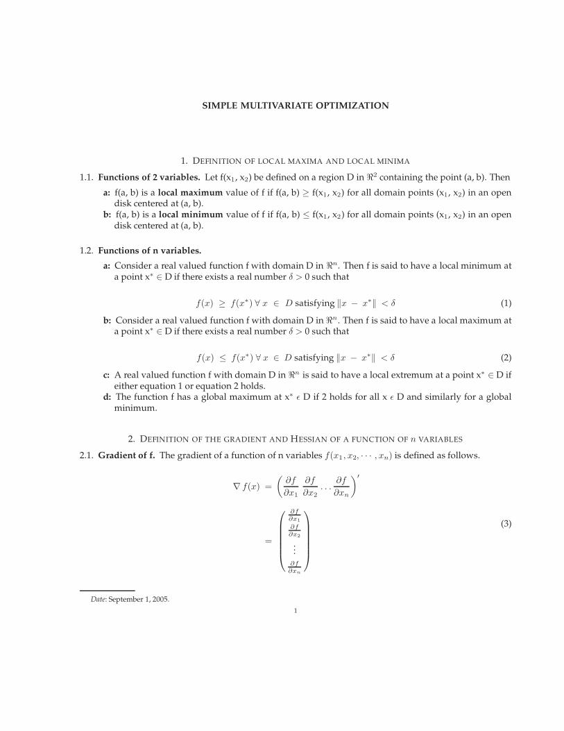
SIMPLE MULTIVARIATE OPTIMIZATION

1. DEFINITION OF LOCAL MAXIMA AND LOCAL MINIMA

1.1. Functions of 2 variables. Let f(x1, x2) be defined on a region D in <2 containing the point (a, b). Then

a: f(a, b) is a local maximum value of f if f(a, b) ≥ f(x1, x2) for all domain points (x1, x2) in an opendisk centered at (a, b).

b: f(a, b) is a local minimum value of f if f(a, b) ≤ f(x1, x2) for all domain points (x1, x2) in an opendisk centered at (a, b).

1.2. Functions of n variables.

a: Consider a real valued function f with domain D in <n. Then f is said to have a local minimum ata point x∗ ∈ D if there exists a real number δ > 0 such that

f(x) ≥ f(x∗) ∀ x ∈ D satisfying ‖x − x∗‖ < δ (1)

b: Consider a real valued function f with domain D in <n. Then f is said to have a local maximum ata point x∗ ∈ D if there exists a real number δ > 0 such that

f(x) ≤ f(x∗) ∀ x ∈ D satisfying ‖x − x∗‖ < δ (2)

c: A real valued function f with domain D in <n is said to have a local extremum at a point x∗ ∈ D ifeither equation 1 or equation 2 holds.

d: The function f has a global maximum at x∗ ε D if 2 holds for all x ε D and similarly for a globalminimum.

2. DEFINITION OF THE GRADIENT AND HESSIAN OF A FUNCTION OF n VARIABLES

2.1. Gradient of f. The gradient of a function of n variables f(x1, x2, · · · , xn) is defined as follows.

∇ f(x) =(

∂f

∂x1

∂f

∂x2. . .

∂f

∂xn

)′

=

∂f∂x1

∂f∂x2

...∂f

∂xn

(3)

Date: September 1, 2005.1

2 SIMPLE MULTIVARIATE OPTIMIZATION

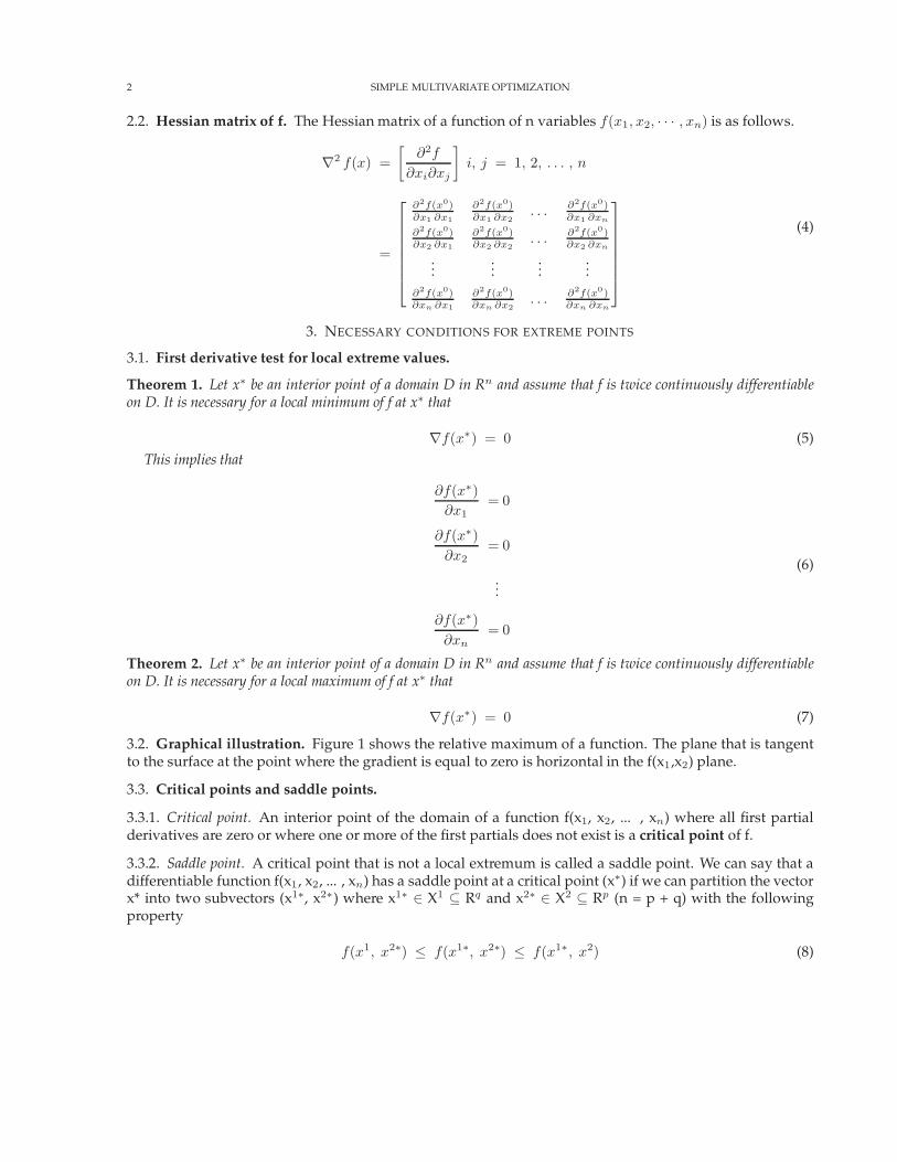
2.2. Hessian matrix of f. The Hessian matrix of a function of n variables f(x1, x2, · · · , xn) is as follows.

∇2 f(x) =[

∂2f

∂xi∂xj

]i, j = 1, 2, . . . , n

=

∂2f(x0)∂x1 ∂x1

∂2f(x0)∂x1 ∂x2

. . . ∂2f(x0)∂x1 ∂xn

∂2f(x0)∂x2 ∂x1

∂2f(x0)∂x2 ∂x2

. . . ∂2f(x0)∂x2 ∂xn

......

......

∂2f(x0)∂xn ∂x1

∂2f(x0)∂xn ∂x2

. . . ∂2f(x0)∂xn ∂xn

(4)

3. NECESSARY CONDITIONS FOR EXTREME POINTS

3.1. First derivative test for local extreme values.

Theorem 1. Let x∗ be an interior point of a domain D in Rn and assume that f is twice continuously differentiableon D. It is necessary for a local minimum of f at x∗ that

∇f(x∗) = 0 (5)This implies that

∂f(x∗)∂x1

= 0

∂f(x∗)∂x2

= 0

...

∂f(x∗)∂xn

= 0

(6)

Theorem 2. Let x∗ be an interior point of a domain D in Rn and assume that f is twice continuously differentiableon D. It is necessary for a local maximum of f at x∗ that

∇f(x∗) = 0 (7)

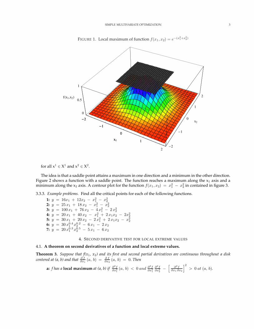
3.2. Graphical illustration. Figure 1 shows the relative maximum of a function. The plane that is tangentto the surface at the point where the gradient is equal to zero is horizontal in the f(x1,x2) plane.

3.3. Critical points and saddle points.

3.3.1. Critical point. An interior point of the domain of a function f(x1, x2, ... , xn) where all first partialderivatives are zero or where one or more of the first partials does not exist is a critical point of f.

3.3.2. Saddle point. A critical point that is not a local extremum is called a saddle point. We can say that adifferentiable function f(x1, x2, ... , xn) has a saddle point at a critical point (x∗) if we can partition the vectorx* into two subvectors (x1∗, x2∗) where x1∗ ∈ X1 ⊆ Rq and x2∗ ∈ X2 ⊆ Rp (n = p + q) with the followingproperty

f(x1, x2∗) ≤ f(x1∗, x2∗) ≤ f(x1∗, x2) (8)

SIMPLE MULTIVARIATE OPTIMIZATION 3

FIGURE 1. Local maximum of function f(x1, x2) = e−(x21+x2

2)

-2

-1

0

1

2

x1

-2

-1

0

1

2

x2

0

0.5

1

fHx1,x2L

-2

-1

0

1x1

for all x1 ∈ X1 and x2 ∈ X2.

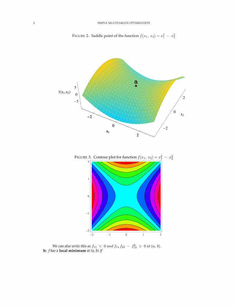
The idea is that a saddle point attains a maximum in one direction and a minimum in the other direction.Figure 2 shows a function with a saddle point. The function reaches a maximum along the x1 axis and aminimum along the x2 axis. A contour plot for the function f(x1, x2) = x2

1 − x22 in contained in figure 3.

3.3.3. Example problems. Find all the critical points for each of the following functions.1: y = 16x1 + 12x2 − x2

1 − x22

2: y = 25 x1 + 18 x2 − x21 − x2

2

3: y = 100 x1 + 76 x2 − 4 x21 − 2 x2

2

4: y = 20 x1 + 40 x2 − x21 + 2 x1x2 − 2x2

2

5: y = 30 x1 + 20 x2 − 2 x21 + 2 x1x2 − x2

2

6: y = 30 x0.41 x0.2

2 − 6 x1 − 2 x2

7: y = 20 x0.31 x0.5

2 − 5 x1 − 6 x2

4. SECOND DERIVATIVE TEST FOR LOCAL EXTREME VALUES

4.1. A theorem on second derivatives of a function and local extreme values.

Theorem 3. Suppose that f(x1, x2) and its first and second partial derivatives are continuous throughout a diskcentered at (a, b) and that ∂ f

∂x1(a, b) = ∂ f

∂x2(a, b) = 0. Then

a: f has a local maximum at (a, b) if ∂2f∂x2

1(a, b) < 0 and ∂2f

∂x21

∂2f∂x2

2−

[∂2f

∂x1 ∂x2

]2

> 0 at (a, b).

4 SIMPLE MULTIVARIATE OPTIMIZATION

FIGURE 2. Saddle point of the function f(x1, x2) = x21 − x2

2

-2

0

2x1

-2

0

2

x2

-5

0

5fHx1,x2L

a

-2

0

2x1

FIGURE 3. Contour plot for function f(x1, x2) = x21 − x2

2

-2 -1 0 1 2

-2

-1

0

1

2

We can also write this as f11 < 0 and f11 f22 − f212 > 0 at (a, b).

b: f has a local minimum at (a, b) if

SIMPLE MULTIVARIATE OPTIMIZATION 5

∂2f∂x2

1(a, b) > 0 and ∂2f

∂x21

∂2f∂x2

2−

[∂2f

∂x1 ∂x2

]2

> 0 at (a, b).

We can also write this as f11 > 0 and f11 f22 − f212 > 0 at (a, b).

c: f has a saddle point at (a, b) if ∂2f∂x2

1

∂2f∂x2

2−

[∂2f

∂x1 ∂x2

]2

< 0 at (a, b).

We can also write this as f11 f22 − f212 < 0 at (a, b).

d: The test is inconclusive at (a, b) if ∂2f∂x2

1

∂2f∂x2

2−

[∂2f

∂x1 ∂x2

]2

= 0 at (a, b).In this case we must find some other way to determine the behavior of f at (a, b).

The expression ∂2f∂x2

1

∂2f∂x2

2−

[∂2f

∂x1 ∂x2

]2

is called the discriminant of f. It is sometimes easier to rememberit by writing it in determinant form

∂2f

∂x21

∂2f

∂x22

−[

∂2f

∂x1 ∂x2

]2

=∣∣∣∣

f11 f12

f21 f22

∣∣∣∣ (9)

The theorem says that if the discriminant is positive at the point (a, b), then the surface curves the sameway in all directions; downwards if f11 < 0, giving rise to a local maximum, and upwards if f11 > 0, givinga local minimum. On the other hand, if the discriminant is negative at (a, b), then the surface curves up insome directions and down in others and we have a saddle point.

4.2. Example problems.

4.2.1. Example 1.

y = 2 − x21 − x2

2

Taking the first partial derivatives we obtain

∂f

∂x1= − 2 x1 = 0 (10a)

∂f

∂x2= − 2 x2 = 0 (10b)

⇒ x1 = 0, x2 = 0 (10c)

Thus we have a critical point at (0,0). Taking the second derivatives we obtain

∂2f

∂x21

= − 2,∂2f

∂x1 ∂x2= 0,

∂2f

∂x2 ∂x1= 0,

∂2f

∂x22

= −2

The discriminant is

∂2f

∂x21

∂2f

∂x22

−[

∂2f

∂x1 ∂x2

]2

=∣∣∣∣f11 f12

f21 f22

∣∣∣∣ =∣∣∣∣−2 00 −2

∣∣∣∣ = (−2) (−2) − (0) (0) = 4.

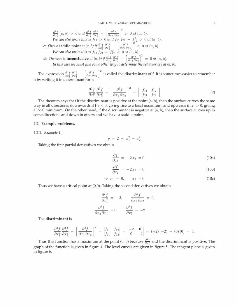
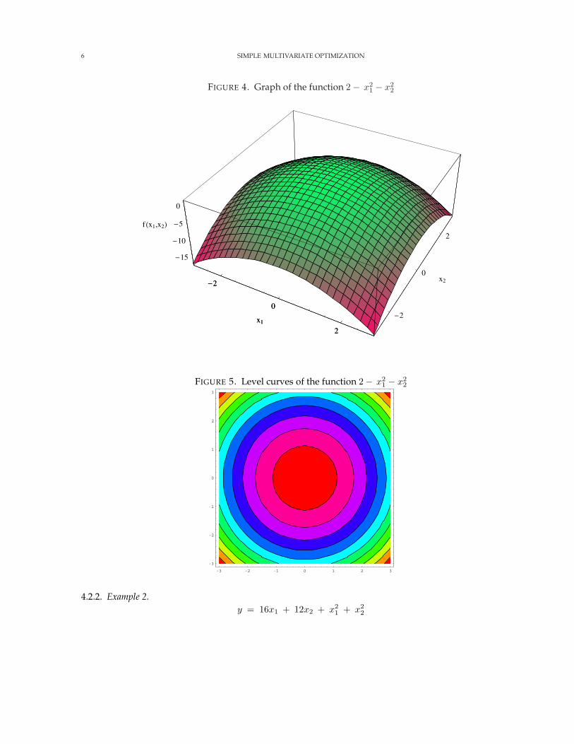
Thus this function has a maximum at the point (0, 0) because ∂2f∂x2

1and the discriminant is positive. The

graph of the function is given in figure 4. The level curves are given in figure 5. The tangent plane is givenin figure 6.

6 SIMPLE MULTIVARIATE OPTIMIZATION

FIGURE 4. Graph of the function 2 − x21 − x2

2

-2

0

2x1

-2

0

2

x2

-15

-10

-5

0

f Hx1,x2L

-2

0

2x1

FIGURE 5. Level curves of the function 2 − x21 − x2

2

-3 -2 -1 0 1 2 3

-3

-2

-1

0

1

2

3

4.2.2. Example 2.y = 16x1 + 12x2 + x2

1 + x22

SIMPLE MULTIVARIATE OPTIMIZATION 7

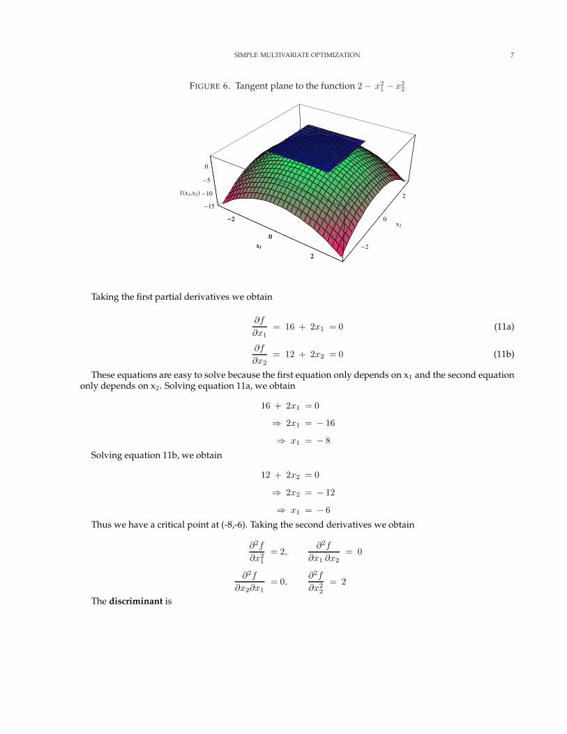
FIGURE 6. Tangent plane to the function 2 − x21 − x2

2

-2

0

2

x1 -2

0

2

x2

-15

-10

-5

0

f Hx1,x2L

-2

0

2

x1

Taking the first partial derivatives we obtain

∂f

∂x1= 16 + 2x1 = 0 (11a)

∂f

∂x2= 12 + 2x2 = 0 (11b)

These equations are easy to solve because the first equation only depends on x1 and the second equationonly depends on x2. Solving equation 11a, we obtain

16 + 2x1 = 0

⇒ 2x1 = − 16

⇒ x1 = − 8

Solving equation 11b, we obtain

12 + 2x2 = 0

⇒ 2x2 = − 12

⇒ x1 = − 6

Thus we have a critical point at (-8,-6). Taking the second derivatives we obtain

∂2f

∂x21

= 2,∂2f

∂x1 ∂x2= 0

∂2f

∂x2∂x1= 0,

∂2f

∂x22

= 2

The discriminant is

8 SIMPLE MULTIVARIATE OPTIMIZATION

∂2f

∂x21

∂2f

∂x22

−[

∂2f

∂x1 ∂x2

]2

=∣∣∣∣f11 f12

f21 f22

∣∣∣∣ =∣∣∣∣2 00 2

∣∣∣∣ = (2) (2) − (0) (0) = 4.

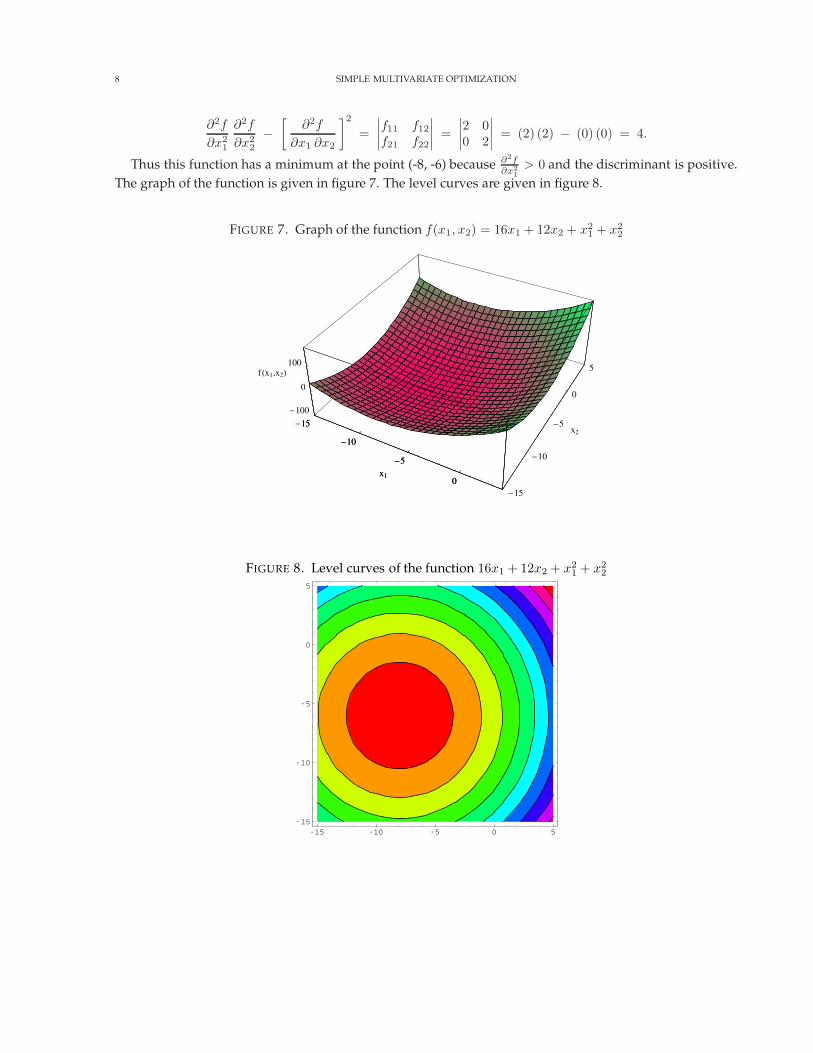
Thus this function has a minimum at the point (-8, -6) because ∂2f∂x2

1> 0 and the discriminant is positive.

The graph of the function is given in figure 7. The level curves are given in figure 8.

FIGURE 7. Graph of the function f(x1, x2) = 16x1 + 12x2 + x21 + x2

2

-15

-10

-5

0x1

-15

-10

-5

0

5

x2

-100

0

100f Hx1,x2L

15

-10

-5

0x1

FIGURE 8. Level curves of the function 16x1 + 12x2 + x21 + x2

2

-15 -10 -5 0 5-15

-10

-5

0

5

SIMPLE MULTIVARIATE OPTIMIZATION 9

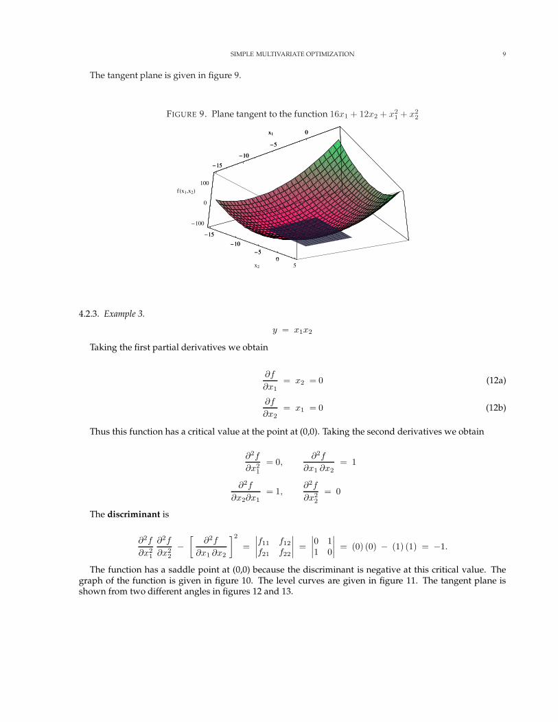
The tangent plane is given in figure 9.

FIGURE 9. Plane tangent to the function 16x1 + 12x2 + x21 + x2

2

-15

-10

-5

0x1

-15

-10-5

05x2

-100

0

100f Hx1,x2L

-15

-10

-5

0x1

-15

-10-5

0

4.2.3. Example 3.

y = x1x2

Taking the first partial derivatives we obtain

∂f

∂x1= x2 = 0 (12a)

∂f

∂x2= x1 = 0 (12b)

Thus this function has a critical value at the point at (0,0). Taking the second derivatives we obtain

∂2f

∂x21

= 0,∂2f

∂x1 ∂x2= 1

∂2f

∂x2∂x1= 1,

∂2f

∂x22

= 0

The discriminant is

∂2f

∂x21

∂2f

∂x22

−[

∂2f

∂x1 ∂x2

]2

=∣∣∣∣f11 f12

f21 f22

∣∣∣∣ =∣∣∣∣0 11 0

∣∣∣∣ = (0) (0) − (1) (1) = −1.

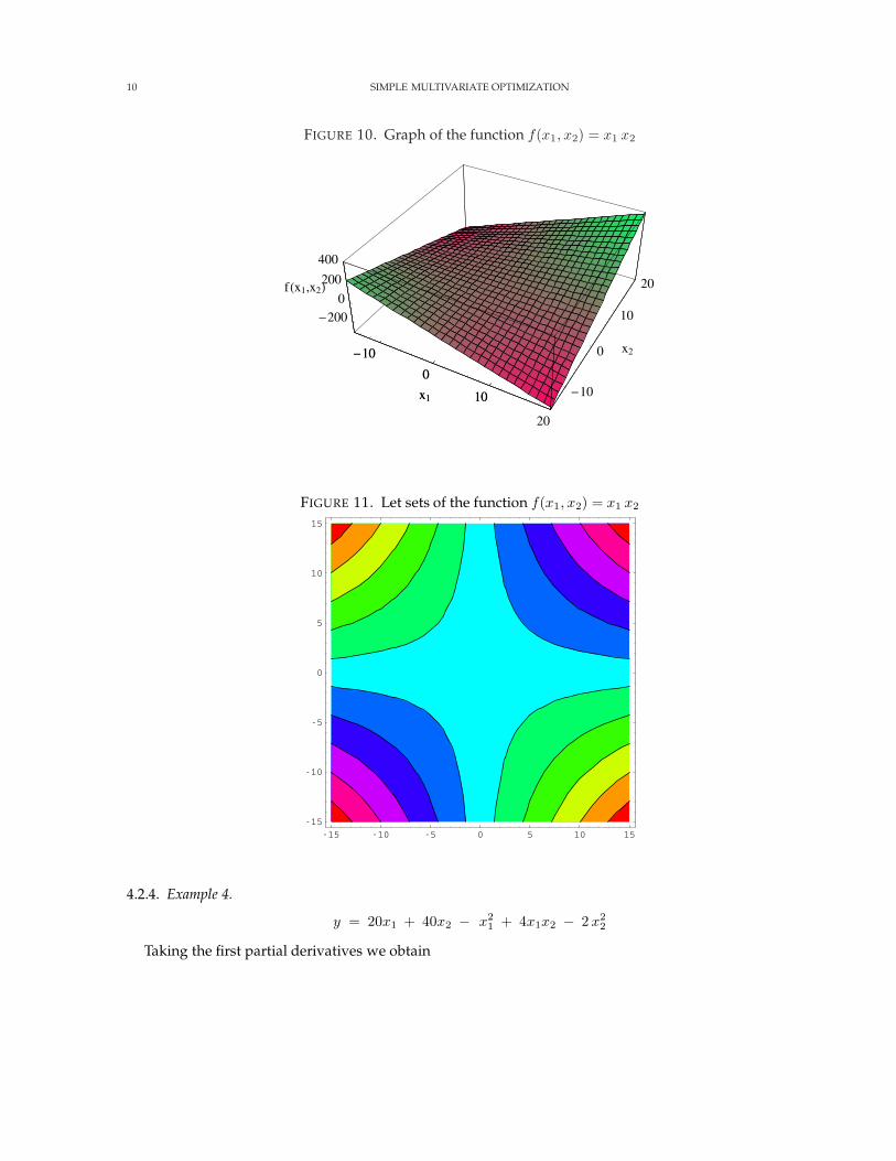
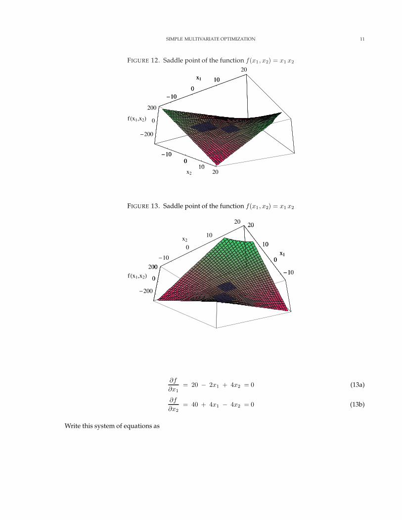
The function has a saddle point at (0,0) because the discriminant is negative at this critical value. Thegraph of the function is given in figure 10. The level curves are given in figure 11. The tangent plane isshown from two different angles in figures 12 and 13.

10 SIMPLE MULTIVARIATE OPTIMIZATION

FIGURE 10. Graph of the function f(x1, x2) = x1 x2

-10

0

10

20

x1 -10

0

10

20

x2

-2000

200

400

f Hx1,x2L

-10

0

10x1

FIGURE 11. Let sets of the function f(x1, x2) = x1 x2

-15 -10 -5 0 5 10 15-15

-10

-5

0

5

10

15

4.2.4. Example 4.

y = 20x1 + 40x2 − x21 + 4x1x2 − 2 x2

2

Taking the first partial derivatives we obtain

SIMPLE MULTIVARIATE OPTIMIZATION 11

FIGURE 12. Saddle point of the function f(x1, x2) = x1 x2

-100

10

20x1

-100

1020x2

-200

0

200

f Hx1,x2L

-100

10x1

-100

10

FIGURE 13. Saddle point of the function f(x1, x2) = x1 x2

-10

0

10

20

x1-10

0

10

20

x2

-200

0

200

f Hx1,x2L -10

0

10

20

x1

0

200

∂f

∂x1= 20 − 2x1 + 4x2 = 0 (13a)

∂f

∂x2= 40 + 4x1 − 4x2 = 0 (13b)

Write this system of equations as

12 SIMPLE MULTIVARIATE OPTIMIZATION

20 − 2x1 + 4x2 = 0 (14a)

40 + 4x1 − 4x2 = 0 (14b)

⇒ 2x1 − 4x2 = 20 (14c)

4x1 − 4x2 = − 40 (14d)

Multiply equation 14c by -2 and add it to equation 14d. First the multiplication

−2(2x1 − 4x2) = − 2(20)

⇒ −4x1 + 8x2 = − 40

Then the addition

−4x1 +8x2 = −40

4x1 −4x2 = −40

−− −− −− −−4x2 = −80

(15)

Now multiply the result in equation 15 by 14

to obtain the system

2x1 −4x2 = 20

x2 = −20(16)

Now multiply the second equation in 16 by 4 and add to the first equation as follows

2x1 −4x2 = 20

4x2 = −80

−− −− −− −−2x1 = −60

(17)

Multiplying the result in equation 17 by 12 we obtain the system

x1 = −30

x2 = −20(18)

Thus we have a critical value at (-30, -20). We obtain the second derivatives by differentiating the systemin equation 13

∂2f

∂x21

= − 2,∂2f

∂x1 ∂x2= 4

∂2f

∂x2 ∂x1= 4,

∂2f

∂x21

= −4

The discriminant is

∂2f

∂x21

∂2f

∂x22

−[

∂2f

∂x1 ∂x2

]2

=∣∣∣∣f11 f12

f21 f22

∣∣∣∣ =∣∣∣∣−2 44 −4

∣∣∣∣ = (−2) (−4) − (4) (4) = −8.

SIMPLE MULTIVARIATE OPTIMIZATION 13

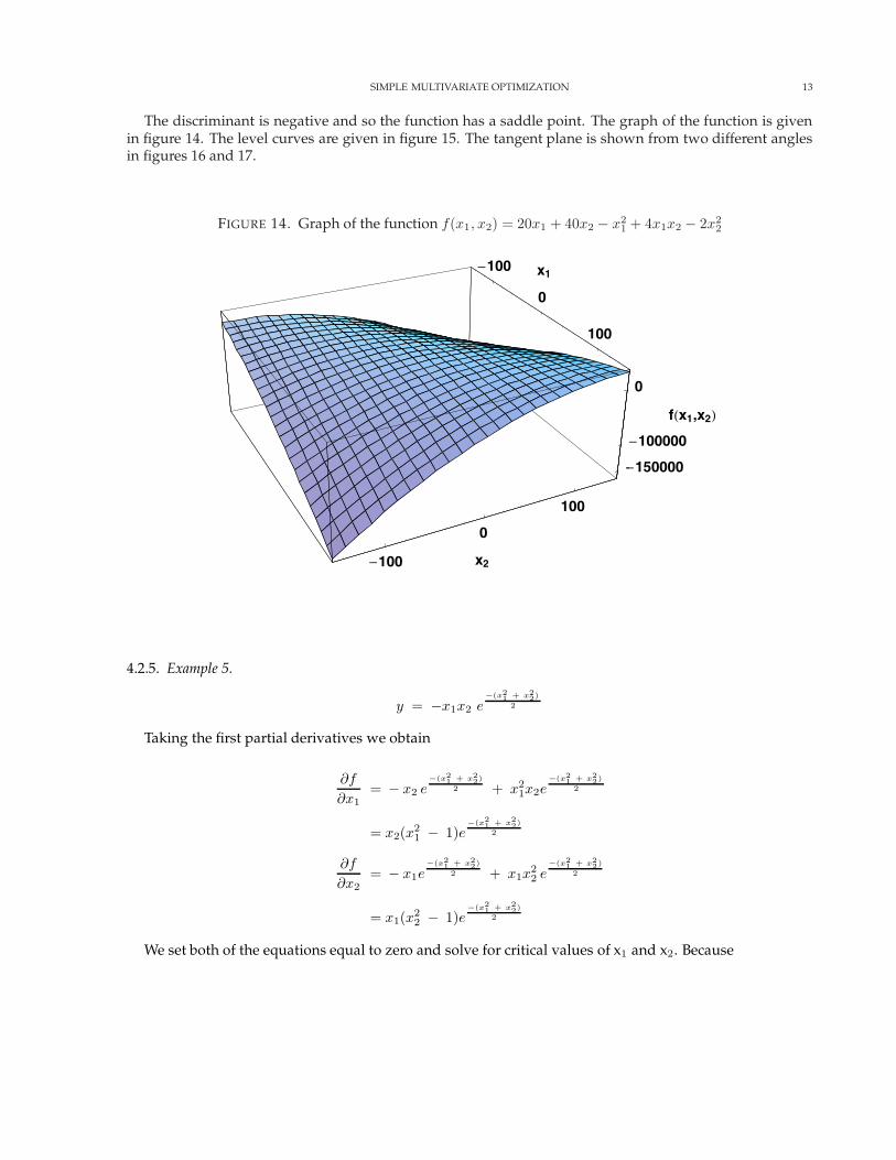
The discriminant is negative and so the function has a saddle point. The graph of the function is givenin figure 14. The level curves are given in figure 15. The tangent plane is shown from two different anglesin figures 16 and 17.

FIGURE 14. Graph of the function f(x1, x2) = 20x1 + 40x2 − x21 + 4x1x2 − 2x2

2

-100

0

100

x1

-100

0

100

x2

-150000

-100000

0

fHx1,x2L

-

-

4.2.5. Example 5.

y = −x1x2 e−(x2

1 + x22)

2

Taking the first partial derivatives we obtain

∂f

∂x1= − x2 e

−(x21 + x2

2)2 + x2

1x2e−(x2

1 + x22)

2

= x2(x21 − 1)e

−(x21 + x2

2)2

∂f

∂x2= − x1e

−(x21 + x2

2)2 + x1x

22 e

−(x21 + x2

2)2

= x1(x22 − 1)e

−(x21 + x2

2)2

We set both of the equations equal to zero and solve for critical values of x1 and x2. Because

14 SIMPLE MULTIVARIATE OPTIMIZATION

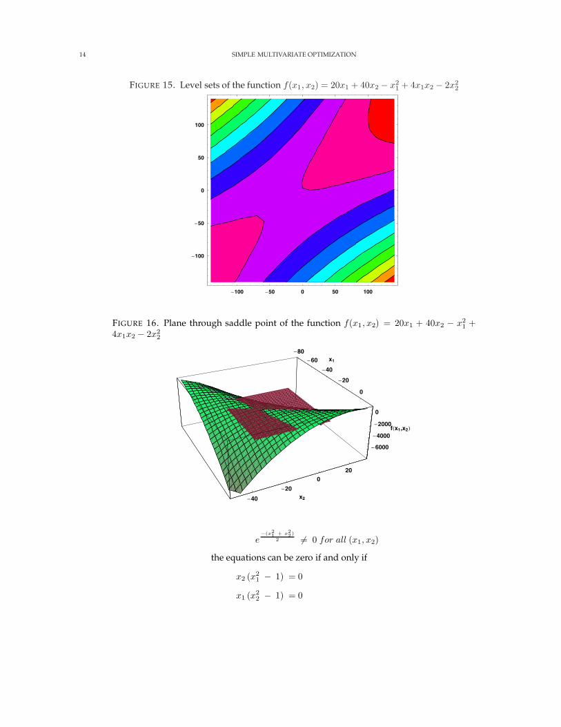
FIGURE 15. Level sets of the function f(x1, x2) = 20x1 + 40x2 − x21 + 4x1x2 − 2x2

2

-100 -50 0 50 100

-100

-50

0

50

100

FIGURE 16. Plane through saddle point of the function f(x1, x2) = 20x1 + 40x2 − x21 +

4x1x2 − 2x22

-80-60

-40

-20

0

x1

-40

-20

020

x2

-6000

-4000

-2000

0

fHx1,x2L

-

e−(x2

1 + x22)

2 6= 0 for all (x1, x2)

the equations can be zero if and only if

x2 (x21 − 1) = 0

x1 (x22 − 1) = 0

SIMPLE MULTIVARIATE OPTIMIZATION 15

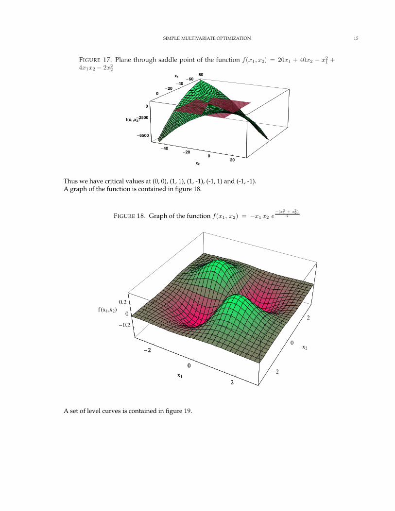
FIGURE 17. Plane through saddle point of the function f(x1, x2) = 20x1 + 40x2 − x21 +

4x1x2 − 2x22

-80-60

-40-20

0

x1

-40-20

020

x2

-6500

-2500

0

fHx1,x2L

Thus we have critical values at (0, 0), (1, 1), (1, -1), (-1, 1) and (-1, -1).A graph of the function is contained in figure 18.

FIGURE 18. Graph of the function f(x1, x2) = −x1 x2 e−(x2

1 + x22)

2

-2

0

2x1

-2

0

2

x2

-0.2

0

0.2f Hx1,x2L

-2

0

2x1

A set of level curves is contained in figure 19.

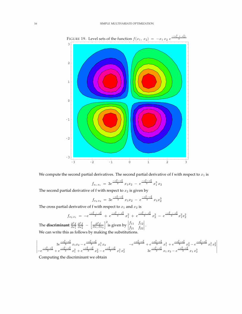
16 SIMPLE MULTIVARIATE OPTIMIZATION

FIGURE 19. Level sets of the function f(x1, x2) = −x1 x2 e−(x2

1 + x22)

2

-3 -2 -1 0 1 2 3-3

-2

-1

0

1

2

3

We compute the second partial derivatives. The second partial derivative of f with respect to x1 is

fx1 x1 = 3e−x2

1−x22

2 x1x2 − e−x2

1−x22

2 x31 x2

The second partial derivative of f with respect to x2 is given by

fx2 x2 = 3e−x2

1−x22

2 x1x2 − e−x2

1−x22

2 x1x32

The cross partial derivative of f with respect to x1 and x2 is

fx2 x1 = −e−x2

1 − x22

2 + e−x2

1 − x22

2 x21 + e

−x21 − x2

22 x2

2 − e−x2

1 − x22

2 x21x

22

The discriminant ∂2f∂x2

1

∂2f∂x2

2−

[∂2f

∂x1 ∂x2

]2

is given by∣∣∣∣f11 f12

f21 f22

∣∣∣∣ .

We can write this as follows by making the substitutions.

∣∣∣∣∣∣3e

−x21−x2

22 x1x2 − e

−x21−x2

22 x3

1 x2 −e−x2

1−x22

2 + e−x2

1−x22

2 x21 + e

−x21−x2

22 x2

2 − e−x2

1−x22

2 x21 x2

2

−e−x2

1−x22

2 + e−x2

1−x22

2 x21 + e

−x21−x2

22 x2

2 − e−x2

1−x22

2 x21 x2

2 3e−x2

1−x22

2 x1 x2 − e−x2

1−x22

2 x1 x32

∣∣∣∣∣∣

Computing the discriminant we obtain

SIMPLE MULTIVARIATE OPTIMIZATION 17

Discriminant =

3e

−x21−x2

22 x1x2 − e

−x21−x2

22 x3

1 x2

3e

−x21−x2

22 x1x2 − e

−x21−x2

22 x1 x3

2

−

−e

−x21−x2

22 + e

−x21−x2

22 x

21 + e

−x21−x2

22 x

22 − e

−x21−x2

22 x

21 x

22

−e

−x21−x2

22 + e

−x21−x2

22 x

21 + e

−x21−x2

22 x

22 − e

−x21−x2

22 x

21x

22

Multiplying out the first term we obtain

term 1 = e−x21−x2

2 x21 (−3 + x2

1) x22 (−3 + x2

2)

= e−x21−x2

2(9 x2

1 x22 − 3 x4

1 x22 − 3 x2

1 x42 + x4

1 x42

)

Multiplying out the second term we obtain

term 2 = e−x21−x2

2 (−1 + x21)

2 (−1 + x22)

2

= e−x21−x2

2(1 − 2x2

1 + x41 − 2x2

2 + 4x21 x2

2 − 2x41 x2

2 + x42 − 2x2

1 x42 + x4

1 x42

)

Subtracting term 2 from term 1 we obtain

Discriminant = e−x21−x2

2(9 x2

1 x22 − 3 x4

1 x22 − 3 x2

1 x42 + x4

1 x42

)

+(−1 + 2x2

1 − x41 + 2x2

2 − 4x21 x2

2 + 2x41 x2

2 − x42 + 2x2

1 x42 − x4

1 x42

)

= e−x21−x2

2(−1 + 5x2

1 x22 − x4

1 x22 − x2

1 x42 + 2x2

1 + 2x22 − x4

1 − x42

)

Because e−x21 − x2

2 > 0 for all (x1, x2), we need only consider the term in parentheses to check the signof the discriminant. Consider each of the cases in turn.

a: Consider the critical point (0, 0). In the case the relevant term is given by(−1 + 5x2

1 x22 − x4

1 x22 − x2

1 x42 + 2x2

1 + 2x22 − x4

1 − x42

)= −1

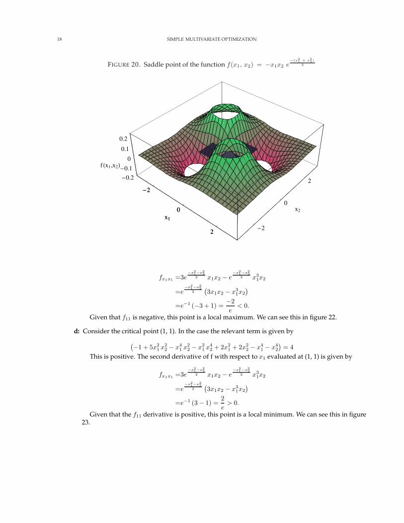
This is negative so this is a saddle point. We can see this in figure 20.

b: Consider the critical point (1, -1). In the case the relevant term is given by(−1 + 5x2

1 x22 − x4

1 x22 − x2

1 x42 + 2x2

1 + 2x22 − x4

1 − x42

)= 4

This is positive. The second derivative of f with respect to x1 evaluated at (1, -1) is given by

fx1x1 =3e−x2

1−x22

2 x1x2 − e−x2

1−x22

2 x31x2

=e−x2

1−x22

2(3x1x2 − x3

1x2

)

=e−1 (−3 + 1) =−2e

< 0.

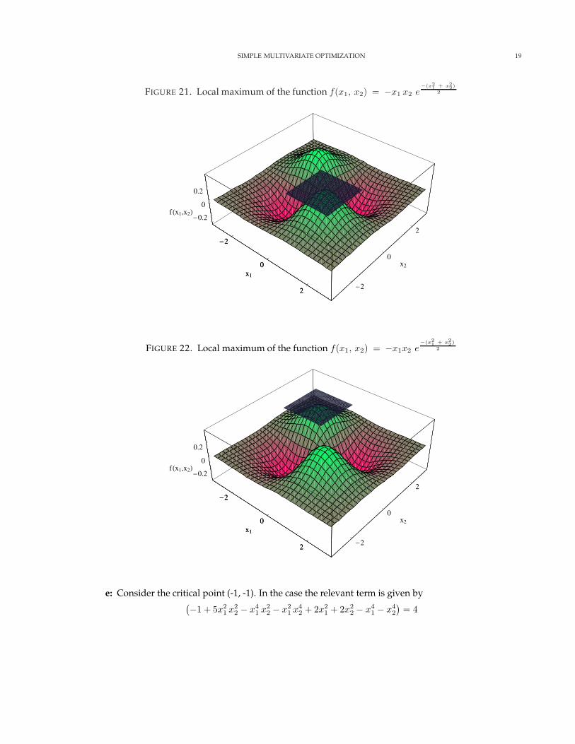
Given that the f11 is negative, this point is a local maximum. We can see this in figure 21.

c: Consider the critical point (-1, 1). In the case the relevant term is given by(−1 + 5x2

1 x22 − x4

1 x22 − x2

1 x42 + 2x2

1 + 2x22 − x4

1 − x42

)= 4

This is positive. The second derivative of x with respect to x1 evaluated at (1, -1) is given by

18 SIMPLE MULTIVARIATE OPTIMIZATION

FIGURE 20. Saddle point of the function f(x1, x2) = −x1x2 e−(x2

1 + x22)

2

-2

0

2

x1

-2

0

2

x2

-0.2

-0.1

0

0.1

0.2

f Hx1,x2L

-2

0

2

x1

fx1x1 =3e−x2

1−x22

2 x1x2 − e−x2

1−x22

2 x31x2

=e−x2

1−x22

2(3x1x2 − x3

1x2

)

=e−1 (−3 + 1) =−2e

< 0.

Given that f11 is negative, this point is a local maximum. We can see this in figure 22.

d: Consider the critical point (1, 1). In the case the relevant term is given by

(−1 + 5x2

1 x22 − x4

1 x22 − x2

1 x42 + 2x2

1 + 2x22 − x4

1 − x42

)= 4

This is positive. The second derivative of f with respect to x1 evaluated at (1, 1) is given by

fx1x1 =3e−x2

1−x22

2 x1x2 − e−x2

1−x22

2 x31x2

=e−x2

1−x22

2(3x1x2 − x3

1x2

)

=e−1 (3 − 1) =2e

> 0.

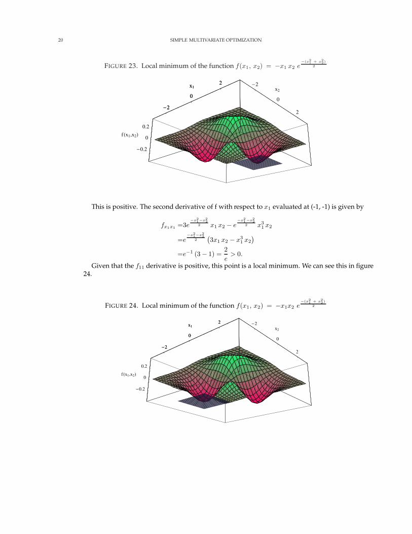
Given that the f11 derivative is positive, this point is a local minimum. We can see this in figure23.

SIMPLE MULTIVARIATE OPTIMIZATION 19

FIGURE 21. Local maximum of the function f(x1, x2) = −x1 x2 e−(x2

1 + x22)

2

-2

0

2

x1

-2

0

2

x2

-0.2

0

0.2

f Hx1,x2L

-2

0

2

x1

FIGURE 22. Local maximum of the function f(x1, x2) = −x1x2 e−(x2

1 + x22)

2

-2

0

2

x1

-2

0

2

x2

-0.2

0

0.2

f Hx1,x2L

-2

0

2

x1

e: Consider the critical point (-1, -1). In the case the relevant term is given by(−1 + 5x2

1 x22 − x4

1 x22 − x2

1 x42 + 2x2

1 + 2x22 − x4

1 − x42

)= 4

20 SIMPLE MULTIVARIATE OPTIMIZATION

FIGURE 23. Local minimum of the function f(x1, x2) = −x1 x2 e−(x2

1 + x22)

2

-2

0

2x1-2

0

2

x2

-0.2

0

0.2

f Hx1,x2L

-2

0

2x1

This is positive. The second derivative of f with respect to x1 evaluated at (-1, -1) is given by

fx1x1 =3e−x2

1−x22

2 x1 x2 − e−x2

1−x22

2 x31 x2

=e−x2

1−x22

2(3x1 x2 − x3

1 x2

)

=e−1 (3 − 1) =2e

> 0.

Given that the f11 derivative is positive, this point is a local minimum. We can see this in figure24.

FIGURE 24. Local minimum of the function f(x1, x2) = −x1x2 e−(x2

1 + x22)

2

-2

0

2x1

-2

0

2

x2

-0.2

0

0.2

f Hx1,x2L

-2

0

2x1

SIMPLE MULTIVARIATE OPTIMIZATION 21

4.3. In-class problems.

a: y = 2x21 + x2

2 − x1x2 − 7 x2

b: y = x22 − x1x2 + 2x1 + x2 + 1

c: y = 16 x1 + 10 x2 − 2 x21 + x1x2 − x2

2

d: y = 4 x1x2 − 2 x21 − x4

2

e: y = 10 x0.41 x0.2

2 − x1 − 2 x2

5. TAYLOR SERIES

5.1. Definition of a Taylor series. Let f be a function with derivatives of all orders throughout some inter-val containing a as an interior point. The Taylor series generated by f at x = a is

∞∑

k=0

fk(a)

k!(x − a)k = f(a) + f ′a)(x − a) +

f ′′(a)

2!(x − a)2 +

f ′′′(a)

3!(x − a)3 + · · · +

fn(a)

n!(x − a)n + · · · (19)

5.2. Definition of a Taylor polynomial. The linearization of a differentiable function f at a point a is thepolynomial

P1(x) = f(a) + f ′(a)(x − a) (20)

For a given a, f(a) and f ′(a) will be constants and we get a linear equation in x. This can be extended tohigher order terms as follows.

Let f be a function with derivatives of order k for k = 1, 2, ... , N in some interval containing a as aninterior point. Then for any integer n from 0 through N, the Taylor polynomial of order n generated by fat x = a is the polynomial

Pn(x) = f(a) + f ′(a) (x − a) +f ′′(a)

2!(x − a)2 + · · · +

fk(a)k!

(x − a)k + · · · +fn(a)

n!(x − a)n (21)

That is, the Taylor polynomial of order n is the Taylor series truncated with the term containing the nthderivative of f. This allows us to approximate a function with polynomials of higher orders.

5.3. Taylor’s theorem.

Theorem 4. If a function f and its first n derivatives f ′, f ′′, . . . , f (n) are continuous on [a, b] or on [b, a], and f(n) isdifferentiable on (a, b) or (b, a), then there exists a number c between a and b such that

f(b) = f(a) + f ′(a) (b − a) +f ′′(a)

2!(b − a)2 + . . . +

fn(a)n!

(b − a)n +fn+1(c)(n + 1)!

(b − a)n+1 (22)

What this says is that we can approximate the function f at the point b by an nth order polynomial

defined at the point a with an error term defined by fn+1 (c)(n+1)! (b − a)n+1. In using Taylor’s theorem we

usually think of a as being fixed and treat b as an independent variable. If we replace b with x we obtainthe following corollary.

Corollary 1. If a function f has derivatives of all orders in an open interval I containing a, then for eachpositive integer n and for each x in I,

22 SIMPLE MULTIVARIATE OPTIMIZATION

f(x) = f(a) + f ′(a)(x − a) +f ′′(a)

2!(x − a)2 + · · · +

fn(a)n!

(x − a)n + Rn(x) ,

where

Rn(x) =fn+1(c)(n + 1)!

(x − a)n+1 for some c between a and x.

(23)

If Rn(x) → 0 as n →∞ for all x in I, then we say that the Taylor series generated by f at x = a converges tof on I.

6. PROOF OF THE SECOND DERIVATIVE TEST FOR LOCAL EXTREME VALUES

Let f(x1, x2) have continuous partial derivatives in the open region R containing a point P(a, b) where∂f∂x1

= ∂f∂x2

= 0. Let h and k be increments small enough to put the point S(a+h, b+k) and the line segmentjoining it to P inside R. We parameterize the line segment PS as

x1 = a + th, x2 = b + tk, 0 ≤ t ≤ 1. (24)Define F(t) as f(a+th, b+tk). In this way F tracks the movement of the function f along the line segment

from P to S. Now differentiate F with respect to t using the chain rule to obtain

F ′(t) =∂f

∂x1

dx1

dt+

∂f

∂x2

dx2

dt= f1h + f2k . (25)

Because ∂f∂x1

and ∂f∂x2

are differentiable, F’ is a differentiable function of t and we have

F ′′(t) = ∂F ′

∂x1

dx1dt

+ ∂F ′

∂x2

dx2dt

= ∂∂x1

(f1 h + f2k) h + ∂∂x2

(f1 h + f2k) k

= h2 f11 + 2 hk f12 + k2 f22,

(26)

where we use the fact that f12 = f21. By the definition of F, which is defined over the interval 0 ≤ t ≤ 1,and the fact that f is continuous over the open region R, it is clear that F and F ′ are continuous on [0, 1] andthat F’ is differentiable on (0, 1). We can then apply Taylor’s formula with n = 2 and a = 0. This will give

F (1) = F (0) + F ′(0) (1 − 0) + F ′′(c)(1 − 0)2

2(27)

Simplifying we obtain

F (1) = F (0) + F ′(0) (1 − 0) + F ′′(c) (1 − 0)2

2

= F (0) + F ′(0) + F ′′(c)2

(28)

for some c between 0 and 1. Now write equation 28 in terms of f. Since t = 1 in equation 28, we obtain fat the point (a+h, b+k) or

f(a + h, b + k) = f(a, b) + hf1(a, b) + kf2 (a, b) + 12 (h2f11 + 2 h k f12 + k2f22)|(a+ch, b+ck) (29)

Because ∂f∂x1

= ∂f∂x2

= 0 at (a, b), equation 29 reduces to

f(a + h, b + k) − f(a, b) =12 (h2 f11 + 2 h k f12 + k2 f22)|(a+ch, b+ck) (30)

The presence of an extremum of f at the point (a, b) is determined by the sign of the left hand side ofequation 30, or f(a+b, b+k) - f(a, b). If [f(a + h, b + k) − f(a, b)] < 0 then the point is a maximum. If

SIMPLE MULTIVARIATE OPTIMIZATION 23

[f(a + h, b + k) − f(a, b)] > 0, the point is a minimum. So if the left hand side (lhs) of equation 20 < 0, wehave a maximum, and if the left hand side of equation 20 > 0, we have a minimum. Specifically,

lhs < 0, f is at a maximum

lhs > 0, f is at a minimum

By equation 30 this is the same as the sign of

Q(c) = (h2f11 + 2 h k f12 + k2 f22)|(a + ch, b+ck) (31)If Q(0) 6= 0, the sign of Q(c) will be the same as the sign of Q(0) for sufficiently small values of h and k.

We can predict the sign of

Q(0) = h2 f11 (a, b) + 2 h k f12 (a, b) + k2 f22 (a, b) (32)from the signs of f11 and f11 f22 − f 2

12 at the point (a, b). Multiply both sides of equation 32 by f11 andrearrange to obtain

f11 Q(0) = f11 (h2 f11 + 2 h k f12 + k2 f22)

= f 211 h2 + 2 h k f11 f12 + k2 f11 f22

= f 211 h2 + 2 h k f11 f12 + k2 f 2

12 − k2 f 212 + k2 f11 f22

= ( h f11 + k f12 )2 − k2 f 212 + k2 f11 f22

= ( h f11 + k f12 )2 + ( f11 f22 − f 212 ) k2

(33)

Now from equation 33 we can see thata: If f11 < 0 and f11 f22 − f 2

12 > 0 at (a, b), then Q(0) < 0 for all sufficiently small values of h andk. This is clear because the right hand side of equation 33 will be positive if the discriminant ispositive. With the right hand side positive, the left hand side must be positive which implies thatwith f11 < 0, Q(0) must also be negative. Thus f has a local maximum at (a, b) because f evaluatedat points close to (a, b) is less than f at (a, b).

b: If f11 > 0 and f11 f22 − f 212 > 0 at (a, b), then Q(0) > 0 for all sufficiently small values of h

and k. This is clear because the right hand side of equation 33 will be positive if the discriminant ispositive. With the right hand side positive, the left hand side must be positive which implies thatwith f11 > 0, Q(0) must also be positive. Thus f has a local minimum at (a, b) because f evaluatedat points close to (a, b) is greater than f at (a, b).

c: If f11 f22 − f 212 < 0 at (a, b), there are combinations of arbitrarily small nonzero values of h and

k for which Q(0) > 0 and other values for which Q(0) < 0. Arbitrarily close to the point P0(a, b,f(a, b)) on the surface y = f(x1, x2) there are points above P0 and points below P0, so f has a saddlepoint at (a, b).

d: If f11 f22 − f 212 = 0 , another test is needed. The possibility that Q(0) can be zero prevents us

from drawing conclusions about the sign of Q(c).