Embed Size (px)
Citation preview
Simplification of CTL Formulaefor Efficient Model Checking of Petri Nets
Frederik Bønneland, Jakob Dyhr, Peter G. Jensen,Mads Johannsen, and Jirı Srba
Department of Computer Science, Aalborg University,Selma Lagerlofs Vej 300, DK-9220 Aalborg East, Denmark
Abstract. We study techniques to overcome the state space explosionproblem in CTL model checking of Petri nets. Classical state space prun-ing approaches like partial order reductions and structural reductions be-come less efficient with the growing size of the CTL formula. The reasonis that the more places and transitions are used as atomic propositionsin a given formula, the more of the behaviour (interleaving) becomesrelevant for the validity of the formula. We suggest several methods toreduce the size of CTL formulae, while preserving their validity. By thesemethods, we significantly increase the benefits of structural and partialorder reductions, as the combination of our techniques can achive up to60 percent average reduction in formulae sizes. The algorithms are imple-mented in the open-source verification tool TAPAAL and we documentthe efficiency of our approach on a large benchmark of Petri net modelsand queries from the Model Checking Contest 2017.
1 Introduction
Model checking [6] of distributed systems, described in high-level formalismslike Petri nets, is often a time and resource consuming task—attributed mainlyto the state space explosion problem. Several techniques like partial order andsymmetry reductions [16,20,21,23,24] and structural reductions [14,18,17] weresuggested for reducing the size of the state space of a given Petri net in needof exploration to verify different logical specifications. These techniques try toprune the searchable state space and their efficiency is to a high degree influencedby the type and size of the logical formula in question. The larger the formula isand the more atomic propositions (querying the number of tokens in places orthe fireability of certain transitions) it has, the less can be pruned away whenexploring the state space and hence the effect of these techniques is reduced. It istherefore desirable to design techniques that can reduce the size of a given logicalformula, while preserving the model checking answer. For practical applicability,it is important that such formula reduction techniques are computationally lessdemanding than the actual state space search.
In this paper, we focus on the well-known logic CTL [5] and describe threemethods for CTL formula simplification, each preserving the logical equivalence
w.r.t. a the given Petri net model. The first two methods rely on standard log-ical equivalences of formulae, while the third one uses state equations of Petrinets and linear programming to recursively traverse the structure of a givenCTL formula. During this process, we identify subformulae that are either triv-ially satisfied or impossible to satisfy, and we replace them with easier to verifyalternatives. We provide an algorithm for performing such a formula simplifi-cation, including the traversal though temporal CTL operators, and prove thecorrectness of our approach.
The formula simplification methods are implemented and fully integratedinto an open-source model checker TAPAAL [10] and its untimed verificationengine verifypn [14]. We document the performance of our tool on the largebenchmark of Petri net models and CTL queries from the Model Checking Con-test 2017 (MCC’17) [15]. The data show that for CTL cardinality queries, weare able to achieve on average 60% of reduction of the query size and about34% of queries are simplified into trivial queries true or false, hence avoidingcompletely the state space exploration. For CTL fireability queries, we achieved50% reduction of the query size and about 10% of queries are simplified intotrue or false. Finally, we compare our simplification algorithm with the one im-plemented in the tool LoLA [26], the winner of MCC’17 in the several categoriesincluding the CTL category, documenting a noticeable performance margin infavour of our approach, both in the number of solved queries purely by the CTLsimplification as well as when CTL verification follows the simplification process.For completeness, we also present the data for pure reachability queries wherethe tool Sara [25] (run parallel with LoLA during MCC’17) performs counterex-ample guided abstraction refinement and contributes to a high number (abouttwice as high as our tool) of solved reachability queries without the need to runLoLA’s state space exploration. Nevertheless, if we also include the actual veri-fication after the formula simplification, TAPAAL now moves 0.4% ahead of thecombined performance of LoLA and Sara.
Related work. Traditionally, the conditions generated by the state equation tech-nique [17] express linear constraints on the number of times the events can occurrelative to other events of the system, and form a necessary condition for markingreachability. State equations were used in [14] as an over-approximation tech-nique for preprocessing of reachability formulae in earlier editions of the modelchecking contest. As the technique can be often inconclusive, extensions of stateequations were studied e.g. in [11] where the authors use traps to increase pre-cision of the method, or in [8] where the state equation technique is extendedto liveness properties. State equations, as a necessary condition for reachability,were also used in other application domains like concurrent programming [1,2].Our work further extends state equations to full CTL logic and improves theprecision of the method by a recursive evaluation of integer linear programs forall subformulae, while employing state equations for each subformula and itsnegation. State equations were also exploited in [22] in order to guide the statespace search based on a minimal solution to the equations. This approach is or-thogonal with ours as it essentially defines a heuristic search strategy that in the
worst case must explore the whole state space. More recently, the state equationtechnique was also applied to the coverability problem for Petri nets [4,12].
Formula rewriting techniques (in order to reduce the size of CTL formulae)are implemented in the tool LoLA [26]. The tool performs formula simplificationby employing subformula rewriting rules that include a subset of the rules de-scribed in Section 3. LoLA also employs the model checking tool Sara [25] thatuses state equations in combination with Counter Example Abstraction Refine-ment (CEGAR) to perform an exact reachability analysis, being able to answerboth reachability and non-reachability questions and hence it is close to being acomplete model checker. Sara shows a very convincing performance on reacha-bility queries, however, in the CTL category, we are able to simplify to true orfalse almost twice as many formulae, compared to the combined performance ofSara and LoLA.
2 Preliminaries
A labelled transition system (LTS) is a tuple TS = (S, A,→) where S is a setof states, A is a set of actions (or labels), and → ⊆ S × A × S is a transition
relation. We write sa−→ s′ whenever (s, a, s′) ∈ → and say that a is enabled in
s. The set of all enabled actions in a state s is denoted en(s). A state s is adeadlock if en(s) = ∅. We write s −→ s′ whenever there is an action a such that
sa−→ s′.A run starting at s0 is any finite or infinite sequence s0
a0−→ s1a1−→ s2
a2−→ · · ·where s0, s1, s2, . . . ∈ S, a0, a1, a2 · · · ∈ A and (si, ai, si+1) ∈ → for all respectivei. We use Π(s) to denote the set of all runs starting at the state s. A run ismaximal if it is either infinite or ends in a state that is a deadlock. Let Πmax (s)denote the set of all maximal runs starting at the state s. A position i in a runπ = s0
a0−→ s1a1−→ s2
a2−→ · · · refers to the state si in the path and is writtenas πi. If π is infinite then any i, 0 ≤ i, is a position in π. Otherwise 0 ≤ i ≤ nwhere sn is the last state in π.
We now define the syntax and semantics of a computation tree logic (CTL) [7]as used in the Model Checking Contest [15]. Let AP be a set of atomic propo-sitions. We evaluate atomic propositions on a given LTS TS = (S, A,→) by thefunction v : S −→ 2AP so that v(s) is the set of atomic propositions satisfied inthe state s ∈ S.
The CTL syntax is given as follows (where α ∈ AP ranges over atomicpropositions):
ϕ ::= true | false | α |deadlock | ϕ1 ∧ ϕ2 | ϕ1 ∨ ϕ2 | ¬ϕ | AXϕ | EXϕ | AFϕ |EFϕ | AGϕ | EGϕ | A(ϕ1Uϕ2) | E (ϕ1Uϕ2) .
We use ΦCTL to denote the set of all CTL formulae. The semantics of a CTLformula ϕ in a state s ∈ S is given in Table 1. We do not use only the minimalset of CTL operators because the query simplification tries to push the negationas far as possible to the atomic predicates. This significantly improves the per-formance of our on-the-fly CTL model checking algorithm and allows for a morerefined query rewriting.
s |= true
s 6|= false
s |= α iff α ∈ v(s)
s |= deadlock iff en(s) = ∅s |= ϕ1 ∧ ϕ2 iff s |= ϕ1 and s |= ϕ2
s |= ϕ1 ∨ ϕ2 iff s |= ϕ1 or s |= ϕ2
s |= ¬ϕ iff s 6|= ϕ
s |= AXϕ iff s′ |= ϕ for all s′ ∈ S s.t. s −→ s′
s |= EXϕ iff there is s′ ∈ S s.t s −→ s′ and s′ |= ϕ
s |= AFϕ iff for all π ∈ Πmax (s) there is a position i in π s.t. πi |= ϕ
s |= EFϕ iff there is π ∈ Πmax (s) and a position i in π s.t. πi |= ϕ
s |= AGϕ iff for all π ∈ Πmax (s) and for all positions i in π we have πi |= ϕ
s |= EGϕ iff there is π ∈ Πmax (s) s.t. for all positions i in π we have πi |= ϕ
s |= A(ϕ1Uϕ2) iff for all π ∈ Πmax (s) there is a position i in π s.t.
πi |= ϕ2 and for all j, 0 ≤ j < i, we have πj |= ϕ1
s |= E(ϕ1Uϕ2) iff there is π ∈ Πmax (s) and there is a position i in π s.t.
πi |= ϕ2 and for all j, 0 ≤ j < i, we have πj |= ϕ1
Table 1: Semantics of CTL formulae
We can now define weighted Petri nets with inhibitor arcs. Let N0 = N∪0be the set of natural numbers including 0 and let N∞ = N ∪ ∞ be the set ofnatural numbers including infinity.
Definition 1 (Petri net). A Petri net is a tuple N = (P, T,W, I) where P andT are finite disjoint sets of places and transitions, W : (P × T )∪ (T × P )→ N0
is the weight function for regular arcs, and I : (P × T ) → N∞ is the weightfunction for inhibitor arcs.
A marking M on N is a function M : P −→ N0 where M(p) denotes thenumber of tokens in the place p. The set of all markings of a Petri net N iswritten as M(N). Let M0 ∈M(N) be a given initial marking of N .
A Petri net N = (P, T,W, I) defines an LTS TS(N) = (S, A,→) where
S =M(N) is the set of all markings, A = T is the set of labels, and Mt−→ M ′
whenever for all p ∈ P we have M(p) < I((p, t)) and M(p) ≥W ((p, t)) such that
M ′(p) = M(p)−W ((p, t)) +W ((t, p)). We inductively extend the relationt−→ to
sequences of transitions w ∈ T ∗ such that Mε−→M and M
wt−→M ′ if Mw−→M ′′
and M ′′t−→ M ′. We write M −→∗ M ′ if there is w ∈ T ∗ such that M
w−→ M ′.By reach(M) = M ′ ∈ M(N) | M −→∗ M ′ we denote the set of all markingsreachable from M .
w
m2
m1s1
i1 f1
s2
i2 f2
wait sync
2
2
2
Fig. 1: A Petri net modelling two synchronizing processes
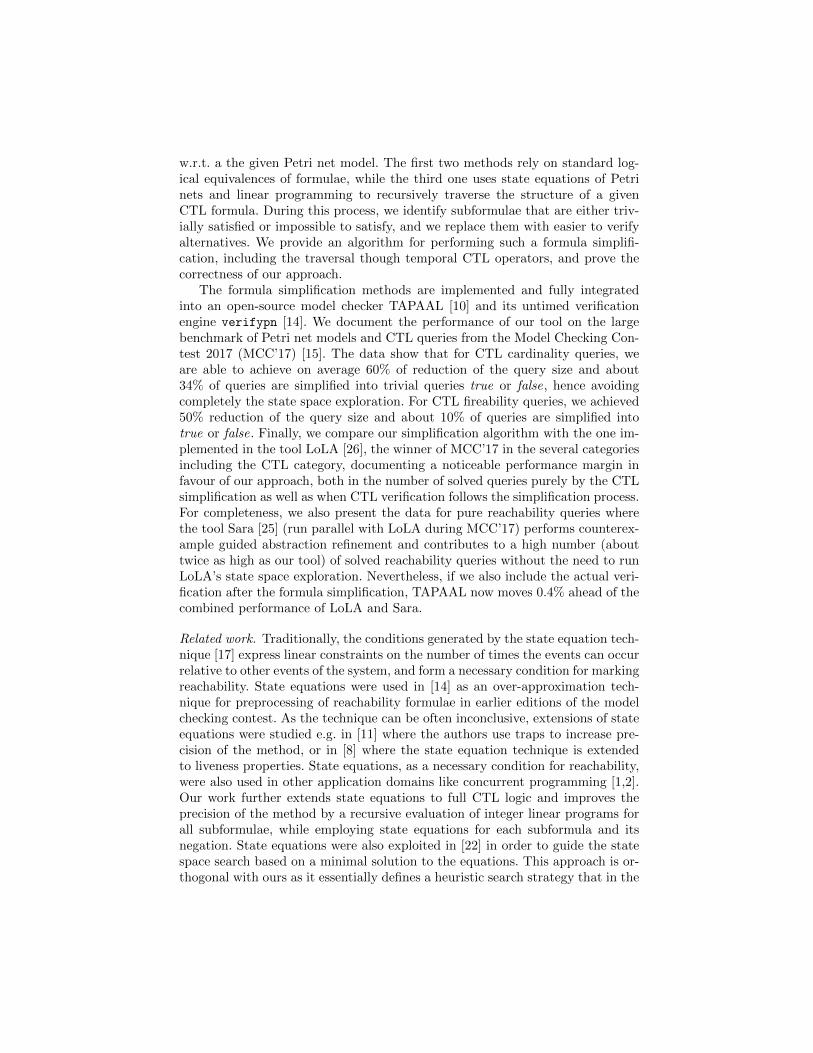
Example 1. Figure 1 illustrates an example of a Petri net where places are drawnas circles, transitions as rectangles, regular arcs as arrows with the weight aslabels (default weight is 1 and arcs with weight 0 are not depicted) and inhibitorarcs are shown as circle-headed arrows (again the default weight is 1 and arcswith weight ∞ are not depicted). The dots inside places represent the numberof tokens (marking). The initial marking in the net can be written by i1i32wdenoting one token in i1, one token in i3 and two tokens in the place w. The netattempts to model two processes that aim to get exclusive access to firing eitherthe transition f1 or f2 (making sure that they cannot be enabled concurrently).Once the first process decides to enable transition f1 by moving the token fromi1 to m1, the second process is not allowed to place a token into m2 due tothe inhibitor arc connection m1 to s2. However, as there is no inhibitor arc inthe order direction, it is possible to reach a deadlock in the net by performingi1i22w
s2−→ i1m2ws1−→ m1m2.
Finally, we fix the set of atomic propositions α (α ∈ AP) for Petri nets asused in the MCC Property Language [15]:
α ::= t | e1 ./ e2
e ::= c | p | e1 ⊕ e2
where t ∈ T , c ∈ N0, ./ ∈ <,≤,=, 6=, >,≥, p ∈ P , and ⊕ ∈ +,−, ∗. Theevaluation function v for a marking M is given as v(M) = t ∈ T | t ∈ en(M)∪e1 ./ e2 | evalM (e1) ./ evalM (e2) where evalM (c) = c, evalM (p) = M(p) andevalM (e1 ⊕ e2) = evalM (e1)⊕ evalM (e2).
Formulae that do not use any atomic predicate t for transition firing anddeadlock are called CTL cardinality formulae and formulae that avoid the use of
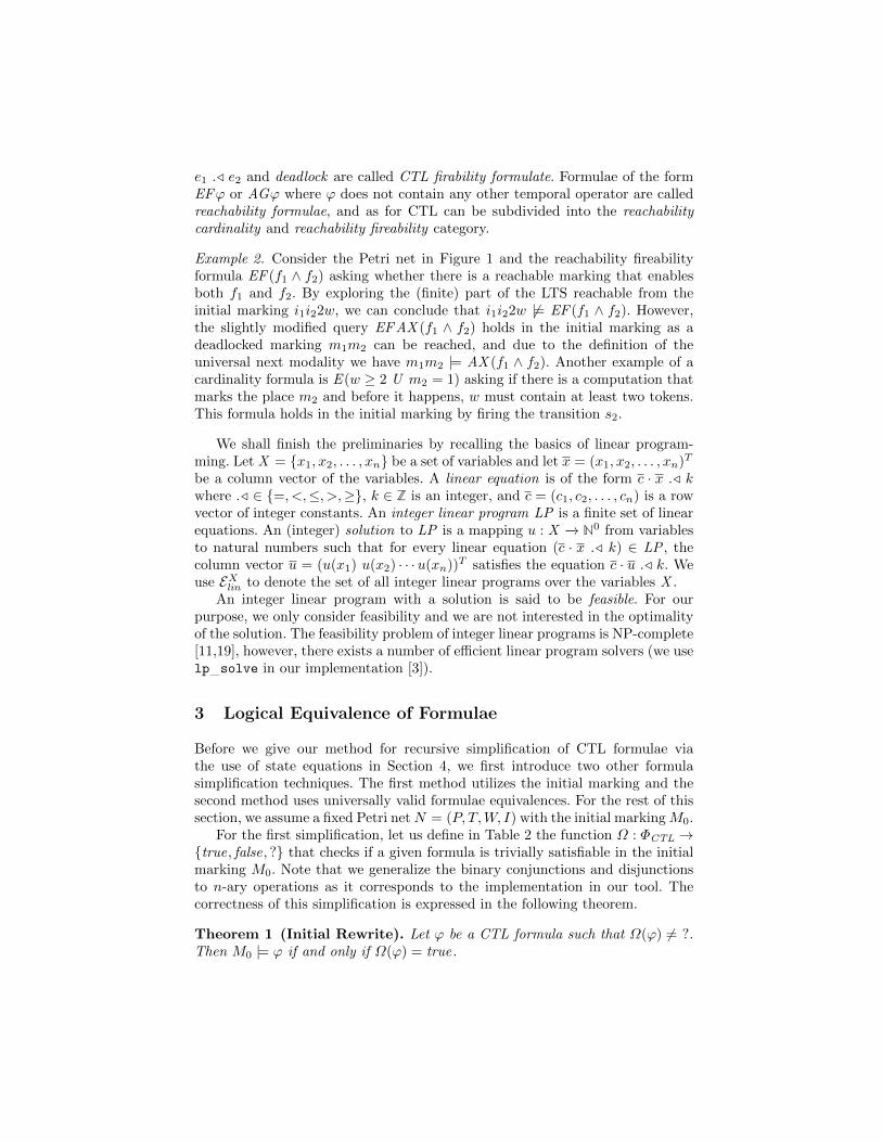
e1 ./ e2 and deadlock are called CTL firability formulate. Formulae of the formEFϕ or AGϕ where ϕ does not contain any other temporal operator are calledreachability formulae, and as for CTL can be subdivided into the reachabilitycardinality and reachability fireability category.
Example 2. Consider the Petri net in Figure 1 and the reachability fireabilityformula EF (f1 ∧ f2) asking whether there is a reachable marking that enablesboth f1 and f2. By exploring the (finite) part of the LTS reachable from theinitial marking i1i22w, we can conclude that i1i22w 6|= EF (f1 ∧ f2). However,the slightly modified query EF AX (f1 ∧ f2) holds in the initial marking as adeadlocked marking m1m2 can be reached, and due to the definition of theuniversal next modality we have m1m2 |= AX (f1 ∧ f2). Another example of acardinality formula is E (w ≥ 2 U m2 = 1) asking if there is a computation thatmarks the place m2 and before it happens, w must contain at least two tokens.This formula holds in the initial marking by firing the transition s2.
We shall finish the preliminaries by recalling the basics of linear program-ming. Let X = x1, x2, . . . , xn be a set of variables and let x = (x1, x2, . . . , xn)T
be a column vector of the variables. A linear equation is of the form c · x ./ kwhere ./ ∈ =, <,≤, >,≥, k ∈ Z is an integer, and c = (c1, c2, . . . , cn) is a rowvector of integer constants. An integer linear program LP is a finite set of linearequations. An (integer) solution to LP is a mapping u : X −→ N0 from variablesto natural numbers such that for every linear equation (c · x ./ k) ∈ LP , thecolumn vector u = (u(x1) u(x2) · · ·u(xn))T satisfies the equation c · u ./ k. Weuse EXlin to denote the set of all integer linear programs over the variables X .
An integer linear program with a solution is said to be feasible. For ourpurpose, we only consider feasibility and we are not interested in the optimalityof the solution. The feasibility problem of integer linear programs is NP-complete[11,19], however, there exists a number of efficient linear program solvers (we uselp solve in our implementation [3]).
3 Logical Equivalence of Formulae
Before we give our method for recursive simplification of CTL formulae viathe use of state equations in Section 4, we first introduce two other formulasimplification techniques. The first method utilizes the initial marking and thesecond method uses universally valid formulae equivalences. For the rest of thissection, we assume a fixed Petri netN = (P, T,W, I) with the initial markingM0.
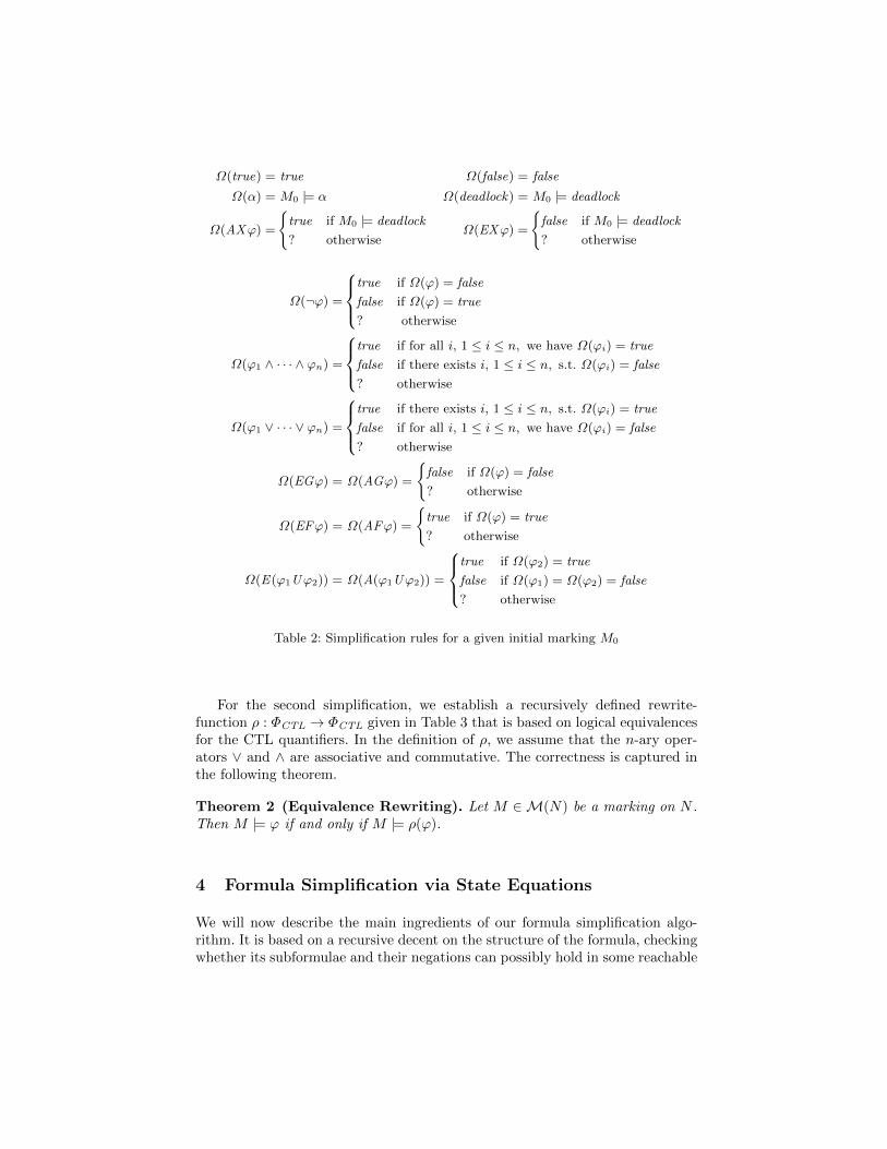
For the first simplification, let us define in Table 2 the function Ω : ΦCTL →true, false, ? that checks if a given formula is trivially satisfiable in the initialmarking M0. Note that we generalize the binary conjunctions and disjunctionsto n-ary operations as it corresponds to the implementation in our tool. Thecorrectness of this simplification is expressed in the following theorem.
Theorem 1 (Initial Rewrite). Let ϕ be a CTL formula such that Ω(ϕ) 6= ?.Then M0 |= ϕ if and only if Ω(ϕ) = true.
Ω(true) = true
Ω(α) = M0 |= α
Ω(AXϕ) =
true if M0 |= deadlock
? otherwise
Ω(false) = false
Ω(deadlock) = M0 |= deadlock
Ω(EXϕ) =
false if M0 |= deadlock
? otherwise
Ω(¬ϕ) =
true if Ω(ϕ) = false
false if Ω(ϕ) = true
? otherwise
Ω(ϕ1 ∧ · · · ∧ ϕn) =
true if for all i, 1 ≤ i ≤ n, we have Ω(ϕi) = true
false if there exists i, 1 ≤ i ≤ n, s.t. Ω(ϕi) = false
? otherwise
Ω(ϕ1 ∨ · · · ∨ ϕn) =
true if there exists i, 1 ≤ i ≤ n, s.t. Ω(ϕi) = true
false if for all i, 1 ≤ i ≤ n, we have Ω(ϕi) = false
? otherwise
Ω(EGϕ) = Ω(AGϕ) =
false if Ω(ϕ) = false
? otherwise
Ω(EFϕ) = Ω(AFϕ) =
true if Ω(ϕ) = true
? otherwise
Ω(E(ϕ1Uϕ2)) = Ω(A(ϕ1Uϕ2)) =
true if Ω(ϕ2) = true
false if Ω(ϕ1) = Ω(ϕ2) = false
? otherwise
Table 2: Simplification rules for a given initial marking M0
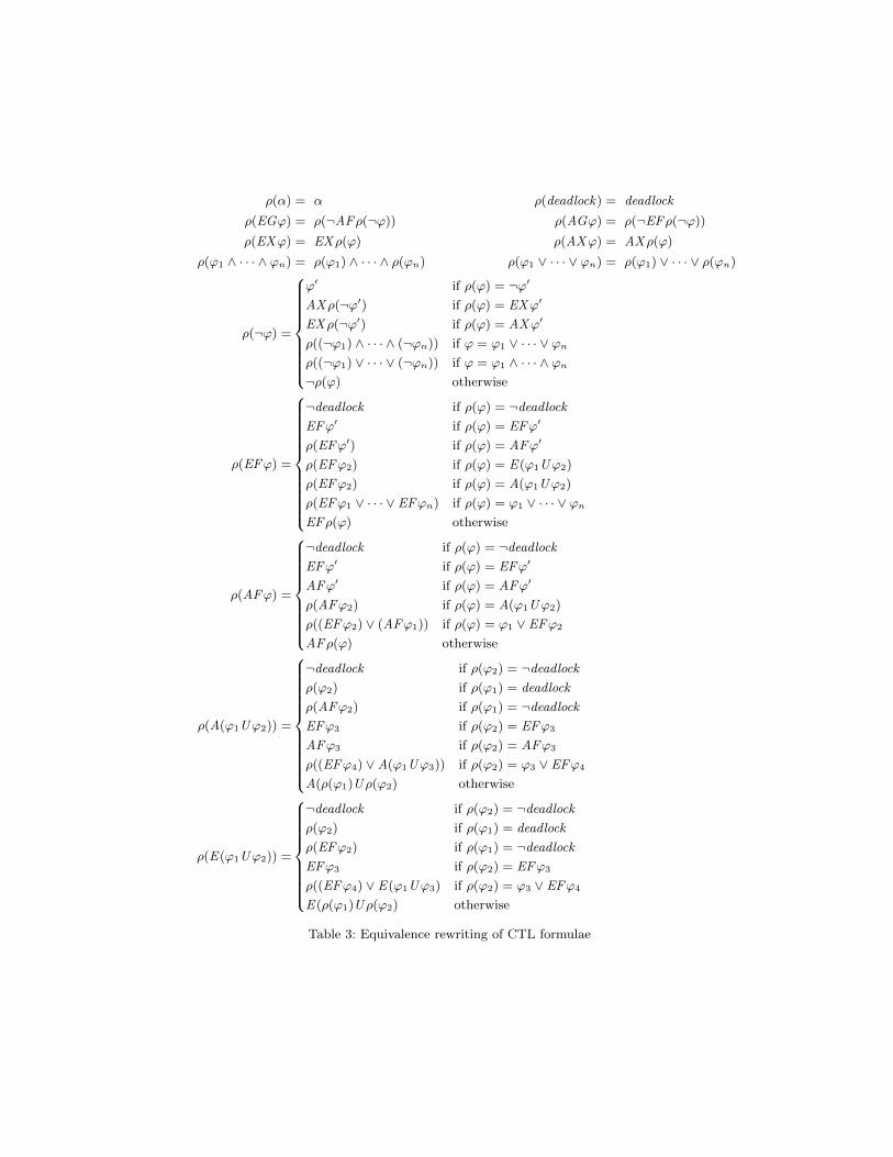
For the second simplification, we establish a recursively defined rewrite-function ρ : ΦCTL → ΦCTL given in Table 3 that is based on logical equivalencesfor the CTL quantifiers. In the definition of ρ, we assume that the n-ary oper-ators ∨ and ∧ are associative and commutative. The correctness is captured inthe following theorem.
Theorem 2 (Equivalence Rewriting). Let M ∈M(N) be a marking on N .Then M |= ϕ if and only if M |= ρ(ϕ).
4 Formula Simplification via State Equations
We will now describe the main ingredients of our formula simplification algo-rithm. It is based on a recursive decent on the structure of the formula, checkingwhether its subformulae and their negations can possibly hold in some reachable
ρ(α) = α
ρ(EGϕ) = ρ(¬AFρ(¬ϕ))
ρ(EXϕ) = EXρ(ϕ)
ρ(ϕ1 ∧ · · · ∧ ϕn) = ρ(ϕ1) ∧ · · · ∧ ρ(ϕn)
ρ(deadlock) = deadlock
ρ(AGϕ) = ρ(¬EFρ(¬ϕ))
ρ(AXϕ) = AXρ(ϕ)
ρ(ϕ1 ∨ · · · ∨ ϕn) = ρ(ϕ1) ∨ · · · ∨ ρ(ϕn)
ρ(¬ϕ) =
ϕ′ if ρ(ϕ) = ¬ϕ′
AXρ(¬ϕ′) if ρ(ϕ) = EXϕ′
EXρ(¬ϕ′) if ρ(ϕ) = AXϕ′
ρ((¬ϕ1) ∧ · · · ∧ (¬ϕn)) if ϕ = ϕ1 ∨ · · · ∨ ϕn
ρ((¬ϕ1) ∨ · · · ∨ (¬ϕn)) if ϕ = ϕ1 ∧ · · · ∧ ϕn
¬ρ(ϕ) otherwise
ρ(EFϕ) =
¬deadlock if ρ(ϕ) = ¬deadlock
EFϕ′ if ρ(ϕ) = EFϕ′
ρ(EFϕ′) if ρ(ϕ) = AFϕ′
ρ(EFϕ2) if ρ(ϕ) = E(ϕ1Uϕ2)
ρ(EFϕ2) if ρ(ϕ) = A(ϕ1Uϕ2)
ρ(EFϕ1 ∨ · · · ∨ EFϕn) if ρ(ϕ) = ϕ1 ∨ · · · ∨ ϕn
EFρ(ϕ) otherwise
ρ(AFϕ) =
¬deadlock if ρ(ϕ) = ¬deadlock
EFϕ′ if ρ(ϕ) = EFϕ′
AFϕ′ if ρ(ϕ) = AFϕ′
ρ(AFϕ2) if ρ(ϕ) = A(ϕ1Uϕ2)
ρ((EFϕ2) ∨ (AFϕ1)) if ρ(ϕ) = ϕ1 ∨ EFϕ2
AFρ(ϕ) otherwise
ρ(A(ϕ1Uϕ2)) =
¬deadlock if ρ(ϕ2) = ¬deadlock
ρ(ϕ2) if ρ(ϕ1) = deadlock
ρ(AFϕ2) if ρ(ϕ1) = ¬deadlock
EFϕ3 if ρ(ϕ2) = EFϕ3
AFϕ3 if ρ(ϕ2) = AFϕ3
ρ((EFϕ4) ∨A(ϕ1Uϕ3)) if ρ(ϕ2) = ϕ3 ∨ EFϕ4
A(ρ(ϕ1)U ρ(ϕ2) otherwise
ρ(E(ϕ1Uϕ2)) =
¬deadlock if ρ(ϕ2) = ¬deadlock
ρ(ϕ2) if ρ(ϕ1) = deadlock
ρ(EFϕ2) if ρ(ϕ1) = ¬deadlock
EFϕ3 if ρ(ϕ2) = EFϕ3
ρ((EFϕ4) ∨ E(ϕ1Uϕ3) if ρ(ϕ2) = ϕ3 ∨ EFϕ4
E(ρ(ϕ1)U ρ(ϕ2) otherwise
Table 3: Equivalence rewriting of CTL formulae
marking (here we use the state equation [11,17] approach) and then propagatingback this information through the Boolean and temporal operators.
t1 p2
2
t23
2
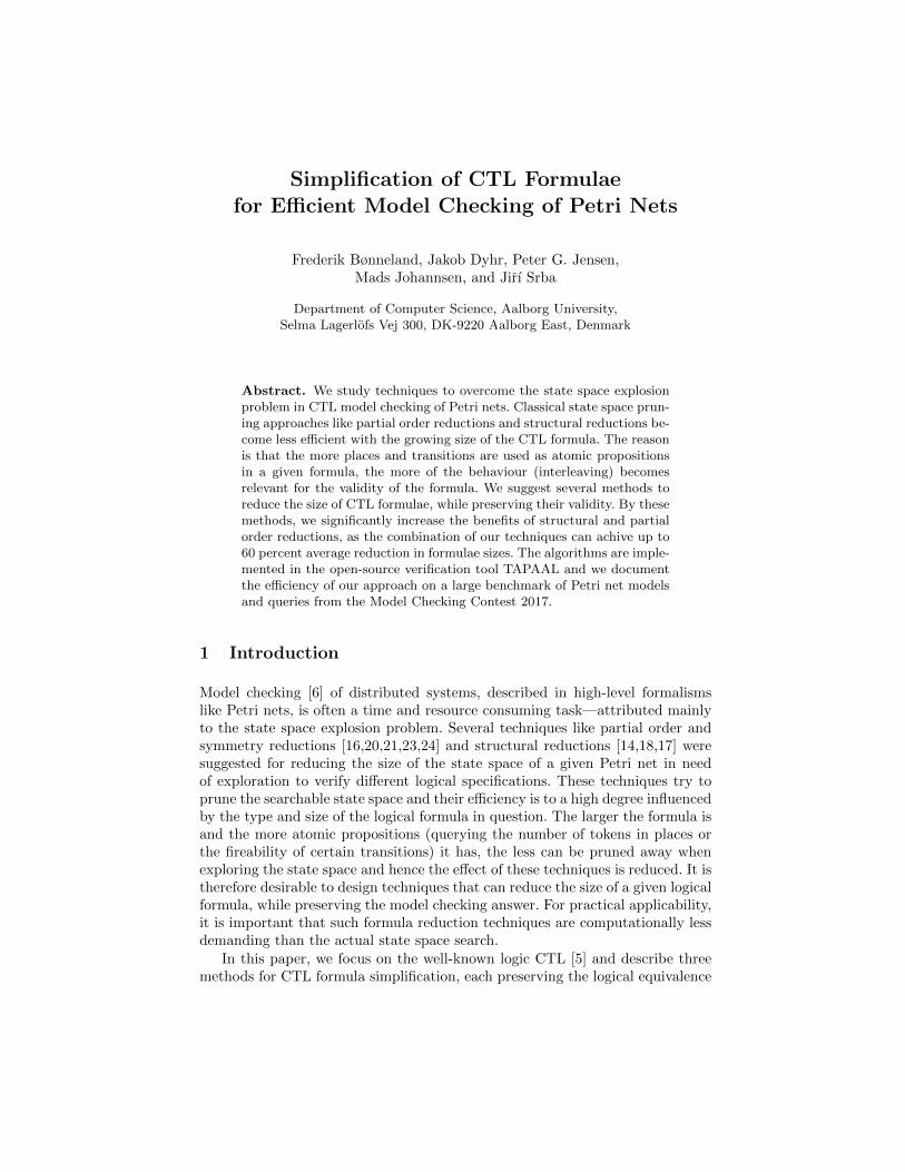
Fig. 2: Example Petri net and initial marking for formula simplification
We use state equations to identify universally true or false subformulae, sim-ilarly as e.g. in [14]. The main novelty is that we extend the approach to dealwith arbitrary arithmetical expressions and repeatedly solve linear programs forsubformulae of the given property so that more significant simplifications canbe achieved (we try to solve the state equations both for the subformula andits negation). As a result, we can simplify more formulae into the trivially validones (true) or invalid ones (false) or we can significantly reduce the size of theformulae which can then speed up the state space exploration.
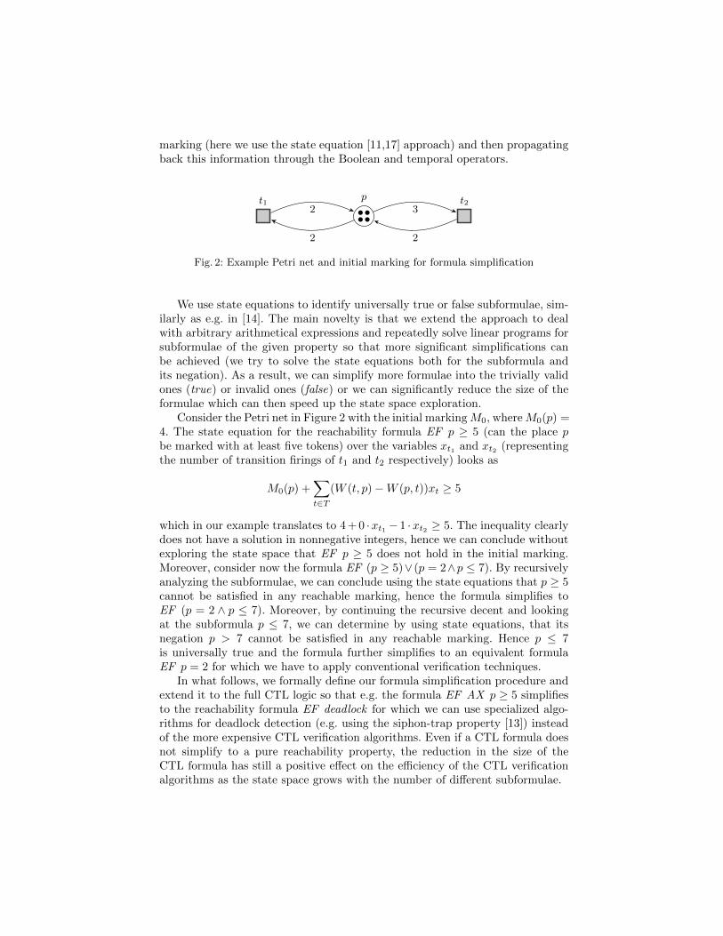
Consider the Petri net in Figure 2 with the initial markingM0, whereM0(p) =4. The state equation for the reachability formula EF p ≥ 5 (can the place pbe marked with at least five tokens) over the variables xt1 and xt2 (representingthe number of transition firings of t1 and t2 respectively) looks as
M0(p) +∑t∈T
(W (t, p)−W (p, t))xt ≥ 5
which in our example translates to 4 + 0 ·xt1 − 1 ·xt2 ≥ 5. The inequality clearlydoes not have a solution in nonnegative integers, hence we can conclude withoutexploring the state space that EF p ≥ 5 does not hold in the initial marking.Moreover, consider now the formula EF (p ≥ 5)∨ (p = 2∧p ≤ 7). By recursivelyanalyzing the subformulae, we can conclude using the state equations that p ≥ 5cannot be satisfied in any reachable marking, hence the formula simplifies toEF (p = 2 ∧ p ≤ 7). Moreover, by continuing the recursive decent and lookingat the subformula p ≤ 7, we can determine by using state equations, that itsnegation p > 7 cannot be satisfied in any reachable marking. Hence p ≤ 7is universally true and the formula further simplifies to an equivalent formulaEF p = 2 for which we have to apply conventional verification techniques.
In what follows, we formally define our formula simplification procedure andextend it to the full CTL logic so that e.g. the formula EF AX p ≥ 5 simplifiesto the reachability formula EF deadlock for which we can use specialized algo-rithms for deadlock detection (e.g. using the siphon-trap property [13]) insteadof the more expensive CTL verification algorithms. Even if a CTL formula doesnot simplify to a pure reachability property, the reduction in the size of theCTL formula has still a positive effect on the efficiency of the CTL verificationalgorithms as the state space grows with the number of different subformulae.
ϕ rewritten ϕ
t p1 ≥W (p1, t) ∧ · · · ∧ pn ≥W (pn, t) ∧p1 < I(p1, t) ∧ · · · ∧ pn < I(pn, t)where P = p1, p2, . . . , pn
e1 6= e2 e1 > e2 ∨ e1 < e2e1 = e2 e1 ≤ e2 ∧ e1 ≥ e2¬(ϕ1 ∧ ϕ2) ¬ϕ1 ∨ ¬ϕ2
¬(ϕ1 ∨ ϕ2) ¬ϕ1 ∧ ¬ϕ2
¬AXϕ EX¬ϕ¬EXϕ AX¬ϕ¬AFϕ EG¬ϕ¬EFϕ AG¬ϕ¬AGϕ EF¬ϕ¬EGϕ AF¬ϕ
Table 4: Rewriting rules
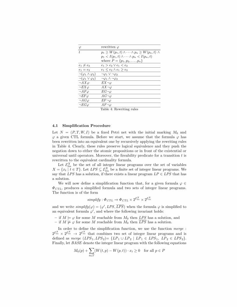
4.1 Simplification Procedure
Let N = (P, T,W, I) be a fixed Petri net with the initial marking M0 andϕ a given CTL formula. Before we start, we assume that the formula ϕ hasbeen rewritten into an equivalent one by recursively applying the rewriting rulesin Table 4. Clearly, these rules preserve logical equivalence and they push thenegation down to either the atomic propositions or in front of the existential oruniversal until operators. Moreover, the fireability predicate for a transition t isrewritten to the equivalent cardinality formula.
Let EXlin be the set of all integer linear programs over the set of variablesX = xt | t ∈ T. Let LPS ⊆ EXlin be a finite set of integer linear programs. Wesay that LPS has a solution, if there exists a linear program LP ∈ LPS that hasa solution.
We will now define a simplification function that, for a given formula ϕ ∈ΦCTL, produces a simplified formula and two sets of integer linear programs.The function is of the form
simplify : ΦCTL −→ ΦCTL × 2EXlin × 2E
Xlin
and we write simplify(ϕ) = (ϕ′,LPS ,LPS ) when the formula ϕ is simplified toan equivalent formula ϕ′, and where the following invariant holds:
– if M |= ϕ for some M reachable from M0 then LPS has a solution, and– if M 6|= ϕ for some M reachable from M0 then LPS has a solution.
In order to define the simplification function, we use the function merge :
2EXlin × 2E
Xlin → 2E
Xlin that combines two set of integer linear programs and is
defined as merge (LPS 1,LPS 2)= LP1 ∪ LP2 | LP1 ∈ LPS 1, LP2 ∈ LPS 2.Finally, let BASE denote the integer linear program with the following equations
M0(p) +∑t∈T
(W (t, p)−W (p, t)) · xt ≥ 0 for all p ∈ P
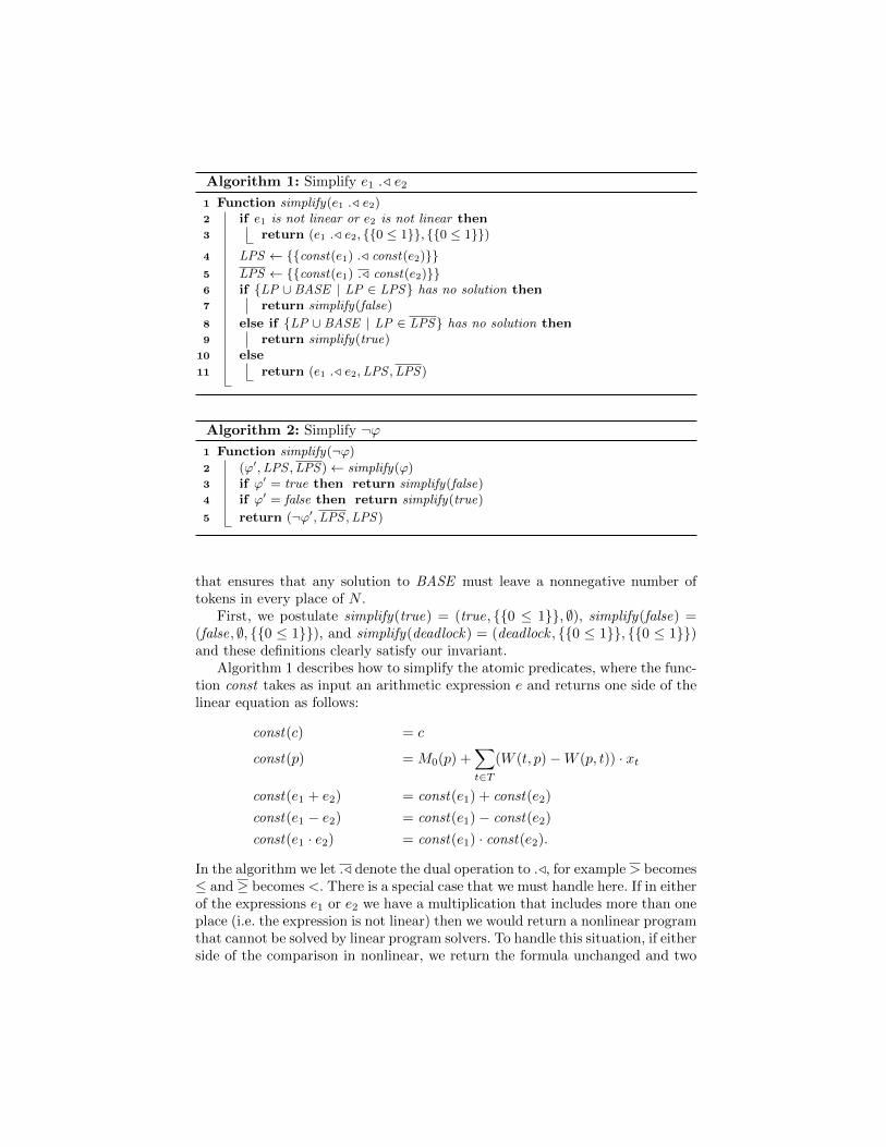
Algorithm 1: Simplify e1 ./ e2
1 Function simplify(e1 ./ e2)2 if e1 is not linear or e2 is not linear then3 return (e1 ./ e2, 0 ≤ 1, 0 ≤ 1)4 LPS ← const(e1) ./ const(e2)5 LPS ← const(e1) ./ const(e2)6 if LP ∪ BASE | LP ∈ LPS has no solution then7 return simplify(false)
8 else if LP ∪ BASE | LP ∈ LPS has no solution then9 return simplify(true)
10 else
11 return (e1 ./ e2,LPS ,LPS)
Algorithm 2: Simplify ¬ϕ1 Function simplify(¬ϕ)
2 (ϕ′,LPS ,LPS)← simplify(ϕ)3 if ϕ′ = true then return simplify(false)4 if ϕ′ = false then return simplify(true)
5 return (¬ϕ′,LPS ,LPS)
that ensures that any solution to BASE must leave a nonnegative number oftokens in every place of N .
First, we postulate simplify(true) = (true, 0 ≤ 1, ∅), simplify(false) =(false, ∅, 0 ≤ 1), and simplify(deadlock) = (deadlock , 0 ≤ 1, 0 ≤ 1)and these definitions clearly satisfy our invariant.
Algorithm 1 describes how to simplify the atomic predicates, where the func-tion const takes as input an arithmetic expression e and returns one side of thelinear equation as follows:
const(c) = c
const(p) = M0(p) +∑t∈T
(W (t, p)−W (p, t)) · xt
const(e1 + e2) = const(e1) + const(e2)
const(e1 − e2) = const(e1)− const(e2)
const(e1 · e2) = const(e1) · const(e2).
In the algorithm we let ./ denote the dual operation to ./, for example > becomes≤ and ≥ becomes <. There is a special case that we must handle here. If in eitherof the expressions e1 or e2 we have a multiplication that includes more than oneplace (i.e. the expression is not linear) then we would return a nonlinear programthat cannot be solved by linear program solvers. To handle this situation, if eitherside of the comparison in nonlinear, we return the formula unchanged and two
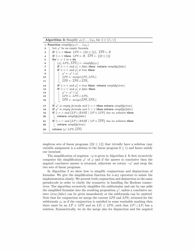
Algorithm 3: Simplify ϕ1♦ . . .♦ϕn for ♦ ∈ ∧,∨1 Function simplify(ϕ1♦ . . .♦ϕn)2 Let ϕ′ be an empty formula.
3 if ♦ = ∧ then LPS ← 0 ≤ 1; LPS ← ∅4 if ♦ = ∨ then LPS ← ∅; LPS ← 0 ≤ 15 for i := 1 to n do
6 (ϕ′i,LPS i,LPS i)← simplify(ϕi)
7 if ♦ = ∧ and ϕ′i = false then return simplify(false)
8 if ♦ = ∧ and ϕ′i 6= true then
9 ϕ′ ← ϕ′ ∧ ϕ′i
10 LPS ← merge(LPS ,LPS i)
11 LPS ← LPS ∪ LPS i
12 if ♦ = ∨ and ϕ′i = true then return simplify(true)
13 if ♦ = ∨ and ϕ′i 6= false then
14 ϕ′ ← ϕ′ ∨ ϕ′i
15 LPS ← LPS ∪ LPS i
16 LPS ← merge(LPS ,LPS i)
17 if ϕ′ is empty formula and ♦ = ∧ then return simplify(true)18 if ϕ′ is empty formula and ♦ = ∨ then return simplify(false)19 if ♦ = ∧ and LP ∪ BASE | LP ∈ LPS has no solution then20 return simplify(false)
21 if ♦ = ∨ and LP ∪ BASE | LP ∈ LPS has no solution then22 return simplify(true)
23 return (ϕ′,LPS ,LPS)
singleton sets of linear programs 0 ≤ 1 that trivially have a solution (anyvariable assignment is a solution to the linear program 0 ≤ 1) and hence satisfyour invariant.
The simplification of negation ¬ϕ is given in Algorithm 2. It first recursivelycomputes the simplification ϕ′ of ϕ and if the answer is conclusive then thenegated conclusive answer is returned, otherwise we return ¬ϕ′ and swap thetwo sets of linear programs.
In Algorithm 3 we show how to simplify conjunctions and disjunctions offormulae. We give the simplification function for n-ary operators to mimic theimplementation closely. We present both conjunction and disjunction in the samepseudocode in order to clarify the symmetry in handling the Boolean connec-tives. The algorithm recursively simplifies the subformulae and one by one addsthe simplified formulae into the resulting proposition ϕ′, unless a conclusive an-swer (true/false) can be given immediately or the subformula can be omitted.Note that for conjunction we merge the current LPS and LPS i returned for thesubformula ϕi as if the conjunction is satisfied in some reachable marking thenthere must be an LP ∈ LPS and an LPi ∈ LPS i such that LP ∪ LPi has asolution. Symmetrically, we do the merge also for disjunction and the negated
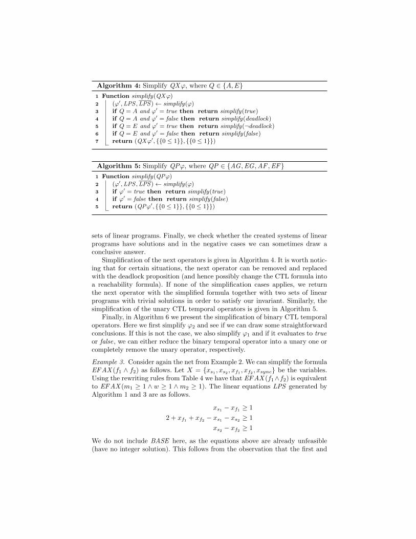
Algorithm 4: Simplify QXϕ, where Q ∈ A,E1 Function simplify(QXϕ)
2 (ϕ′,LPS ,LPS)← simplify(ϕ)3 if Q = A and ϕ′ = true then return simplify(true)4 if Q = A and ϕ′ = false then return simplify(deadlock)5 if Q = E and ϕ′ = true then return simplify(¬deadlock)6 if Q = E and ϕ′ = false then return simplify(false)7 return (QXϕ′, 0 ≤ 1, 0 ≤ 1)
Algorithm 5: Simplify QPϕ, where QP ∈ AG ,EG ,AF ,EF1 Function simplify(QPϕ)
2 (ϕ′,LPS ,LPS)← simplify(ϕ)3 if ϕ′ = true then return simplify(true)4 if ϕ′ = false then return simplify(false)5 return (QPϕ′, 0 ≤ 1, 0 ≤ 1)
sets of linear programs. Finally, we check whether the created systems of linearprograms have solutions and in the negative cases we can sometimes draw aconclusive answer.
Simplification of the next operators is given in Algorithm 4. It is worth notic-ing that for certain situations, the next operator can be removed and replacedwith the deadlock proposition (and hence possibly change the CTL formula intoa reachability formula). If none of the simplification cases applies, we returnthe next operator with the simplified formula together with two sets of linearprograms with trivial solutions in order to satisfy our invariant. Similarly, thesimplification of the unary CTL temporal operators is given in Algorithm 5.
Finally, in Algorithm 6 we present the simplification of binary CTL temporaloperators. Here we first simplify ϕ2 and see if we can draw some straightforwardconclusions. If this is not the case, we also simplify ϕ1 and if it evaluates to trueor false, we can either reduce the binary temporal operator into a unary one orcompletely remove the unary operator, respectively.
Example 3. Consider again the net from Example 2. We can simplify the formulaEF AX (f1 ∧ f2) as follows. Let X = xs1 , xs2 , xf1 , xf2 , xsync be the variables.Using the rewriting rules from Table 4 we have that EF AX (f1∧f2) is equivalentto EF AX (m1 ≥ 1 ∧ w ≥ 1 ∧m2 ≥ 1). The linear equations LPS generated byAlgorithm 1 and 3 are as follows.
xs1 − xf1 ≥ 1
2 + xf1 + xf2 − xs1 − xs2 ≥ 1
xs2 − xf2 ≥ 1
We do not include BASE here, as the equations above are already unfeasible(have no integer solution). This follows from the observation that the first and
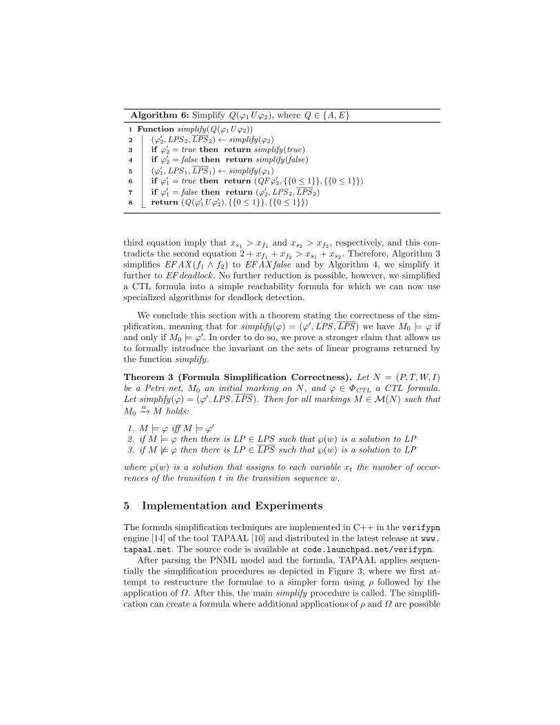
Algorithm 6: Simplify Q(ϕ1Uϕ2), where Q ∈ A,E1 Function simplify(Q(ϕ1Uϕ2))
2 (ϕ′2,LPS2,LPS2)← simplify(ϕ2)
3 if ϕ′2 = true then return simplify(true)
4 if ϕ′2 = false then return simplify(false)
5 (ϕ′1,LPS1,LPS1)← simplify(ϕ1)
6 if ϕ′1 = true then return (QFϕ′
2, 0 ≤ 1, 0 ≤ 1)7 if ϕ′
1 = false then return (ϕ′2,LPS2,LPS2)
8 return (Q(ϕ′1Uϕ′
2), 0 ≤ 1, 0 ≤ 1)
third equation imply that xs1 > xf1 and xs2 > xf2 , respectively, and this con-tradicts the second equation 2 + xf1 + xf2 > xs1 + xs2 . Therefore, Algorithm 3simplifies EF AX (f1 ∧ f2) to EF AX false and by Algorithm 4, we simplify itfurther to EF deadlock . No further reduction is possible, however, we simplifieda CTL formula into a simple reachability formula for which we can now usespecialized algorithms for deadlock detection.
We conclude this section with a theorem stating the correctness of the sim-plification, meaning that for simplify(ϕ) = (ϕ′,LPS ,LPS ) we have M0 |= ϕ ifand only if M0 |= ϕ′. In order to do so, we prove a stronger claim that allows usto formally introduce the invariant on the sets of linear programs returned bythe function simplify .
Theorem 3 (Formula Simplification Correctness). Let N = (P, T,W, I)be a Petri net, M0 an initial marking on N , and ϕ ∈ ΦCTL a CTL formula.Let simplify(ϕ) = (ϕ′,LPS ,LPS ). Then for all markings M ∈ M(N) such that
M0w−→M holds:
1. M |= ϕ iff M |= ϕ′
2. if M |= ϕ then there is LP ∈ LPS such that ℘(w) is a solution to LP3. if M 6|= ϕ then there is LP ∈ LPS such that ℘(w) is a solution to LP
where ℘(w) is a solution that assigns to each variable xt the number of occur-rences of the transition t in the transition sequence w.
5 Implementation and Experiments
The formula simplification techniques are implemented in C++ in the verifypnengine [14] of the tool TAPAAL [10] and distributed in the latest release at www.tapaal.net. The source code is available at code.launchpad.net/verifypn.
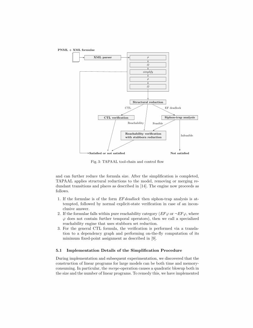
After parsing the PNML model and the formula, TAPAAL applies sequen-tially the simplification procedures as depicted in Figure 3, where we first at-tempt to restructure the formulae to a simpler form using ρ followed by theapplication of Ω. After this, the main simplify procedure is called. The simplifi-cation can create a formula where additional applications of ρ and Ω are possible
XML parser
PNML + XML formulae
ρ
Ω
simplify
ρ
Ω
Structural reduction
CTL verification
CTL
Siphon-trap analysis
EF deadlock
Reachability verificationwith stubborn reduction
Reachability Feasible
Not satisfied
Infeasible
Satisfied or not satisfied
Fig. 3: TAPAAL tool-chain and control flow
and can further reduce the formula size. After the simplification is completed,TAPAAL applies structural reductions to the model, removing or merging re-dundant transitions and places as described in [14]. The engine now proceeds asfollows.
1. If the formulae is of the form EF deadlock then siphon-trap analysis is at-tempted, followed by normal explicit-state verification in case of an incon-clusive answer.
2. If the formulae falls within pure reachability category (EFϕ or ¬EFϕ, whereϕ does not contain further temporal operators), then we call a specializedreachability engine that uses stubborn set reduction.
3. For the general CTL formula, the verification is performed via a transla-tion to a dependency graph and performing on-the-fly computation of itsminimum fixed-point assignment as described in [9].
5.1 Implementation Details of the Simplification Procedure
During implementation and subsequent experimentation, we discovered that theconstruction of linear programs for large models can be both time and memory-consuming. In particular, the merge-operation causes a quadratic blowup both inthe size and the number of linear programs. To remedy this, we have implemented
CTL Cardinality
Algorithm Solved % Solved Reachability % Reachability % Reduction
Ω 117 2.3 1834 36.6 27.2ρ 7 0.1 1437 28.7 24.1simplify 1437 28.7 2425 48.4 45.7all 1724 34.4 2993 59.8 60.3
CTL Fireability
Ω 194 3.9 1701 34.0 27.1ρ 0 0.0 1319 26.3 30.0simplify 255 5.1 1422 28.4 11.0all 495 9.9 2022 40.4 49.7
Table 5: Formula simplification for CTL cardinality and fireability
a “lazy” construction of the linear programs—similar to lazy evaluation knownfrom functional programming languages. Instead of computing the full set oflinear programs up front, we simply remember the basic linear programs andthe tree of operations making up the merged or unioned linear program. Usingthis construction, we then extract a single linear program on demand, and thusavoid the up-front time and memory overhead of computing the merge and unionoperations at the call time.
5.2 Experimental Setup
To evaluate the performance of our approach, we conduct two series of experi-ments on the models and formulae from MCC’17 [15]. First, we investigate theeffect of the three different simplification methods proposed in this paper alongwith their combination as depicted in Figure 3. In the second experiment we com-pare the performance of our simplification algorithms to those used by LoLA,the winner of MCC’17. We also conduct a full run of the verification enginesafter the formula simplification in order to assess the impact of the simplifica-tion on the state space search. All experiments were run on AMD Opteron 6376Processors, restricted to 14 GB of memory on 313 P/T nets from the MCC’17benchmark. Each category contains 16 different queries which yields a total of5008 executions for a given category.
5.3 Evaluation of Formula Simplification Techniques
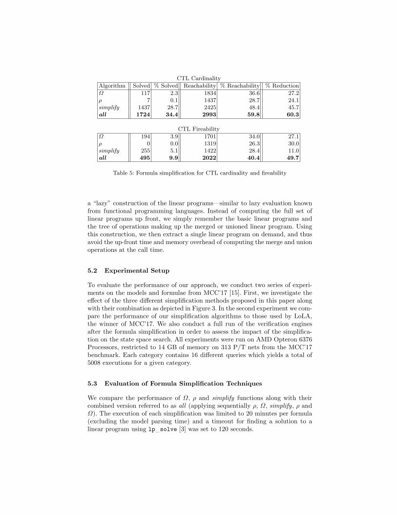
We compare the performance of Ω, ρ and simplify functions along with theircombined version referred to as all (applying sequentially ρ, Ω, simplify , ρ andΩ). The execution of each simplification was limited to 20 minutes per formula(excluding the model parsing time) and a timeout for finding a solution to alinear program using lp solve [3] was set to 120 seconds.
CTL Simplification Only
TAPAAL LoLA LoLA+Sara
Solved % Solved Solved % Solved Solved % Solved
Cardinality 1724 34 236 5 904 18Fireability 495 10 173 3 488 10Total 2219 22 409 4 1392 14
CTL Simplification Followed by Verification
Cardinality 4232 85 3634 73 3810 76Fireability 3712 74 3663 73 3690 74Total 7944 79 7297 73 7500 75
Table 6: Tool comparison on CTL formulae
Table 5 reports the numbers (and percentages) of formulae that were solved(simplified to either true or false), the number of formulae converted from acomplex CTL formula into a pure reachability formula and the average formulareduction in percentages (where the formula size before and after the reductionsis measured as a number of nodes in its parse tree).
We can observe that the combination of our techniques simplifies about 34%of cardinality queries and 10% of fireability queries into true or false, while a sig-nificant number of queries are simplified from CTL formula into pure reachabilityproblems (60% of cardinality queries and 40% of fireability ones). The averagereduction in the query size is 60% for cardinality and 50% for fireability queries.The results are encouraging, though the performance on fireability formulae isconsiderably worse than for cardinality formulae. The reason is that fireabilitypredicates are translated into Boolean combinations of cardinality predicates andthe expanded formulae are less suitable for the simplification procedures due totheir increased size. This is also reflected by the time it took to compute thesimplification. For CTL cardinality, half of the simplifications terminate in lessthan 0.05 seconds, 75% simplifications terminate in less than 0.98 seconds and90% of simplifications terminate in less than 9.46 seconds. The correspondingnumbers for CTL fireability are 0.22 seconds, 13.70 seconds and 538.34 seconds.
5.4 Comparison with LoLA
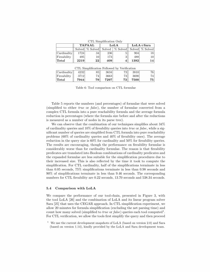
We compare the performance of our tool-chain, presented in Figure 3, withthe tool LoLA [26] and the combination of LoLA and its linear program solverSara [25] that uses the CEGAR approach. In CTL simplification experiment, weallow 20 minutes for formula simplification (excluding the net parsing time) andcount how many solved (simplified to true or false) queries each tool computed1.For CTL verification, we allow the tools first simplify the query and then proceed
1 We use the current development snapshots of LoLA (based on version 2.0) and Sara(based on version 1.14), kindly provided by the LoLA and Sara development team.
Reachability Simplification Only
TAPAAL LoLA LoLA+Sara
Solved % Solved Solved % Solved Solved % Solved
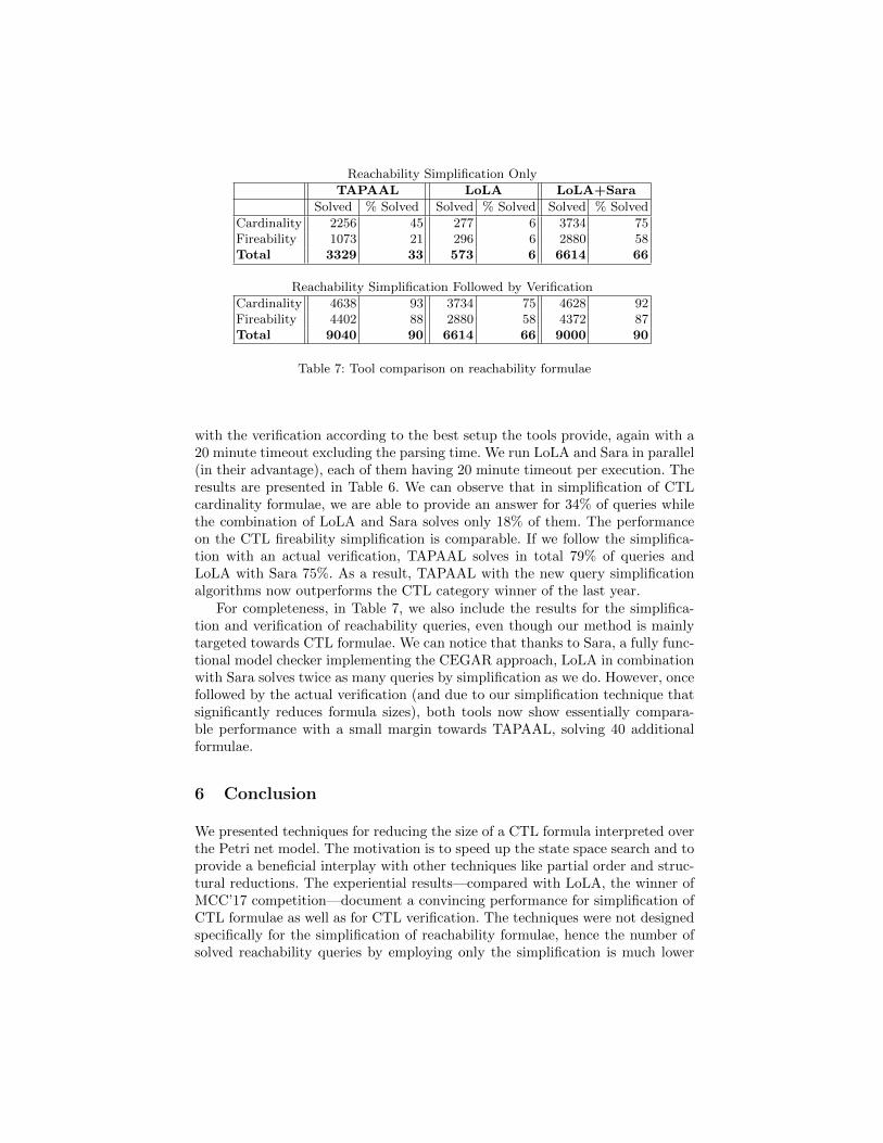
Cardinality 2256 45 277 6 3734 75Fireability 1073 21 296 6 2880 58Total 3329 33 573 6 6614 66
Reachability Simplification Followed by Verification
Cardinality 4638 93 3734 75 4628 92Fireability 4402 88 2880 58 4372 87Total 9040 90 6614 66 9000 90
Table 7: Tool comparison on reachability formulae
with the verification according to the best setup the tools provide, again with a20 minute timeout excluding the parsing time. We run LoLA and Sara in parallel(in their advantage), each of them having 20 minute timeout per execution. Theresults are presented in Table 6. We can observe that in simplification of CTLcardinality formulae, we are able to provide an answer for 34% of queries whilethe combination of LoLA and Sara solves only 18% of them. The performanceon the CTL fireability simplification is comparable. If we follow the simplifica-tion with an actual verification, TAPAAL solves in total 79% of queries andLoLA with Sara 75%. As a result, TAPAAL with the new query simplificationalgorithms now outperforms the CTL category winner of the last year.
For completeness, in Table 7, we also include the results for the simplifica-tion and verification of reachability queries, even though our method is mainlytargeted towards CTL formulae. We can notice that thanks to Sara, a fully func-tional model checker implementing the CEGAR approach, LoLA in combinationwith Sara solves twice as many queries by simplification as we do. However, oncefollowed by the actual verification (and due to our simplification technique thatsignificantly reduces formula sizes), both tools now show essentially compara-ble performance with a small margin towards TAPAAL, solving 40 additionalformulae.
6 Conclusion
We presented techniques for reducing the size of a CTL formula interpreted overthe Petri net model. The motivation is to speed up the state space search and toprovide a beneficial interplay with other techniques like partial order and struc-tural reductions. The experiential results—compared with LoLA, the winner ofMCC’17 competition—document a convincing performance for simplification ofCTL formulae as well as for CTL verification. The techniques were not designedspecifically for the simplification of reachability formulae, hence the number ofsolved reachability queries by employing only the simplification is much lower
than that by the specialized tools like Sara (being in fact a complete modelchecker). However, when combined with the state space search followed afterthe formula simplification, the benefits of our techniques become apparent aswe now solve 40 additional formulae compared to the combined performance ofLoLA and Sara.
The simplification procedure is less efficient for CTL fireability queries thanfor CTL cardinality queries. This is the case both for our tool as well as LoLAand Sara. The reason is that we do not handle fireability predicates directlyand unfold them into Boolean combination of cardinality predicates. This oftenresults in significant explosion in query sizes. The future work will focus on over-coming this limitation and possibly handling the fireability predicates directlyin the engine.
Acknowledgements. We would like to thank Karsten Wolf and Torsten Liebkefrom Rostock University for providing us with the development snapshot of thelatest version of LoLA and for their help with setting up the tool and answeringour questions. The last author is partially affiliated with FI MU, Brno.
References
1. G.S. Avrunin, U.A. Buy, and J.C. Corbett. Integer programming in the analysis ofconcurrent systems. In International Conference on Computer Aided Verification(CAV’91), volume 575 of LNCS, pages 92–102. Springer, 1991.
2. G.S. Avrunin, U.A. Buy, J.C. Corbett, L.K. Dillon, and J.C. Wileden. Auto-mated analysis of concurrent systems with the constrained expression toolset. IEEETransactions on Software Engineering, 17(11):1204–1222, 1991.
3. M. Berkelaar, K. Eikland, P. Notebaert, et al. lpsolve: Open source (mixed-integer)linear programming system. Eindhoven U. of Technology, 2004.
4. M. Blondin, A. Finkel, C. Haase, and S. Haddad. Approaching the CoverabilityProblem Continuously. In Tools and Algorithms for the Construction and Analysisof Systems, volume 9636 of LNCS, pages 480–496. Springer, 2016.
5. E.M. Clarke and E.A. Emerson. Design and synthesis of synchronization skeletonsusing branching-time temporal logic. In Logic of Programs, volume 131 of LNCS,pages 52–71. Springer, 1982.
6. E.M. Clarke, E.A Emerson, and J. Sifakis. Model checking: algorithmic verificationand debugging. Communications of the ACM, 52(11):74–84, 2009.
7. E.M. Clarke, E.A. Emerson, and A.P. Sistla. Automatic verification of finite-state concurrent systems using temporal logic specifications. ACM Transactionson Programming Languages and Systems (TOPLAS), 8(2):244–263, 1986.
8. J.C. Corbett and G.S. Avrunin. Using integer programming to verify general safetyand liveness properties. Formal Methods in System Design, 6(1):97–123, 1995.
9. A.E. Dalsgaard, S. Enevoldsen, P. Fogh, L.S. Jensen, T.S. Jepsen, I. Kaufmann,K.G. Larsen, S.M. Nielsen, M.Chr. Olesen, S. Pastva, and J. Srba. Extended de-pendency graphs and efficient distributed fixed-point computation. In Proceedingsof the 38th International Conference on Application and Theory of Petri Nets andConcurrency (Petri Nets’17), volume 10258 of LNCS, pages 139–158. Springer-Verlag, 2017.
10. A. David, L. Jacobsen, M. Jacobsen, K.Y. Jørgensen, M.H. Møller, and J. Srba.TAPAAL 2.0: Integrated development environment for timed-arc Petri nets. In In-ternational Conference on Tools and Algorithms for the Construction and Analysisof Systems, volume 7214 of LNCS, pages 492–497. Springer, 2012.
11. J. Esparza and S. Melzer. Verification of safety properties using integer program-ming: Beyond the state equation. Formal Methods in System Design, 16(2):159–189, 2000.
12. T. Geffroy, J. Leroux, and G. Sutre. Occam’s Razor Applied to the Petri NetCoverability Problem. In Reachability Problems, volume 9899 of LNCS, pages 77–89. Springer, 2016.
13. M.H.T. Hack. Analysis of production schemata by Petri nets. Technical report,DTIC Document, 1972.
14. J.F. Jensen, T. Nielsen, L.K. Oestergaard, and J. Srba. TAPAAL and Reacha-bility Analysis of P/T Nets. In Transactions on Petri Nets and Other Models ofConcurrency XI, volume 9930 of LNCS, pages 307–318. Springer, 2016.
15. F. Kordon, H. Garavel, L.M. Hillah, F. Hulin-Hubard, B. Berthomieu, G. Cia-rdo, M. Colange, S. Dal Zilio, E. Amparore, M. Beccuti, T. Liebke, J. Mei-jer, A. Miner, C. Rohr, J. Srba, Y. Thierry-Mieg, J. van de Pol, andK. Wolf. Complete Results for the 2017 Edition of the Model Checking Contest.http://mcc.lip6.fr/2017/results.php, June 2017.
16. L.M. Kristensen, K. Schmidt, and A. Valmari. Question-guided stubborn set meth-ods for state properties. Formal Methods in System Design, 29(3):215–251, 2006.
17. T. Murata. Petri nets: Properties, analysis and applications. Proceedings of theIEEE, 77(4):541–580, 1989.
18. T. Murata and J.Y. Koh. Reduction and expansion of live and safe marked graphs.IEEE Transactions on Circuits and Systems, 27(1):68–70, 1980.
19. G.L. Nemhauser and L.A. Wolsey. Integer programming and combinatorial opti-mization. Wiley, Chichester. GL Nemhauser, MWP Savelsbergh, GS Sigismondi(1992). Constraint Classification for Mixed Integer Programming Formulations.COAL Bulletin, 20:8–12, 1988.
20. K. Schmidt. Stubborn sets for standard properties. In International Conference onApplication and Theory of Petri nets, volume 1639 of LNCS, pages 46–65. Springer,1999.
21. K. Schmidt. Integrating low level symmetries into reachability analysis. In Inter-national Conference on Tools and Algorithms for the Construction and Analysis ofSystems, volume 1785 of LNCS, pages 315–330. Springer, 2000.
22. K. Schmidt. Narrowing Petri net state spaces using the state equation. FundamentaInformaticae, 47(3-4):325–335, 2001.
23. A. Valmari. Stubborn sets for reduced state space generation. In InternationalConference on Application and Theory of Petri Nets, volume 483 of LNCS, pages491–515. Springer, 1989.
24. A. Valmari and H. Hansen. Stubborn set intuition explained. In Transactions onPetri Nets and Other Models of Concurrency XII, volume 10470 of LNCS, pages140–165. Springer, 2017.
25. H. Wimmel and K. Wolf. Applying CEGAR to the Petri net state equation.In International Conference on Tools and Algorithms for the Construction andAnalysis of Systems, volume 6605 of LNCS, pages 224–238. Springer, 2011.
26. K. Wolf. Running LoLA 2.0 in a Model Checking Competition. In Transactionson Petri Nets and Other Models of Concurrency XI, volume 9930 of LNCS, pages274–285. Springer, 2016.
A Proof of Theorem 1
Proof. The proof proceeds by structural induction on ϕ.
ϕ = true: Trivial.ϕ = false: Trivial.ϕ = α: Trivial.ϕ = deadlock : Trivial.ϕ = ϕ1 ∧ · · · ∧ ϕn: For all i ∈ 1, . . . , n, we know by the structural induction
hypothesis that if Ω(ϕi) 6= ? then M0 |= ϕi iff Ω(ϕi) = true. Assume thatΩ(ϕ) 6= ? is true. We need to show the following two implications: (1) ifM0 |=ϕ1∧· · ·∧ϕn then Ω(ϕ1∧· · ·∧ϕn) = true, and (2) if Ω(ϕ1∧· · ·∧ϕn) = truethen M0 |= ϕ1 ∧ · · · ∧ ϕn.– Implication (1): Assume M0 |= ϕ1 ∧ · · · ∧ ϕn. Then for all i ∈ 1, . . . , n
we must have that M0 |= ϕi. Assume for the sake of contradiction thatthere exists i ∈ 1, . . . , n s.t. Ω(ϕi) = false. Then by the inductionhypothesis we have M0 6|= ϕi, which is a contradiction. Therefore wemust have Ω(ϕi) 6= false for all i ∈ 1, . . . , n, and from the definition ofΩ(ϕ) in Table 2 we have Ω(ϕ) 6= false. By assumption we have Ω(ϕ) 6= ?,leaving only Ω(ϕ1 ∧ · · · ∧ ϕn) = true as the conclusion.
– Implication (2): Assume Ω(ϕ) = true. Then we have Ω(ϕi) = true forall i ∈ 1, . . . , n, from the definition of Ω(ϕ) in Table 2. Due to theinduction hypothesis we have M0 |= ϕi for all i and M0 |= ϕ1 ∧ · · · ∧ ϕnfollows from the semantics of ϕ1 ∧ · · · ∧ ϕn.
ϕ = ϕ1 ∨ · · · ∨ ϕn: This case is analogous to the conjunction case.ϕ = AXϕ′: Assume that Ω(ϕ) 6= ? is true. Since we by assumption have Ω(ϕ) 6=
?, and Ω(ϕ) = false can never occur due to the definition of Ω(ϕ) in Table 2,we must have M0 |= deadlock and Ω(AXϕ′) = true. If M0 |= deadlock thenM0 |= AXϕ′ trivially follows from the semantics of AXϕ′. We therefore haveM0 |= AXϕ′ iff Ω(AXϕ′) = true follows.
ϕ = EXϕ′: This case is analogous to the AXϕ′ case.ϕ = EGϕ′: By structural induction we have if Ω(ϕ′) 6= ? then M0 |= ϕ′ iffΩ(ϕ′) = true. Assume that Ω(ϕ) 6= ? is true. Since we by assumption haveΩ(ϕ) 6= ?, and Ω(ϕ) = true can never occur due to the definition of Ω(ϕ)in Table 2, we must have Ω(ϕ′) = false and Ω(EGϕ′) = false. Due to theinduction hypothesis we have M0 6|= ϕ′, and M0 6|= EGϕ′ follows from thesemantics of EGϕ′. We therefore have M0 |= EGϕ′ iff Ω(EGϕ′) = truefollows.
ϕ = AGϕ′: This case is analogous to the EGϕ′ case.ϕ = EFϕ′: By structural induction we have if Ω(ϕ′) 6= ? then M0 |= ϕ′ iffΩ(ϕ′) = true. Assume that Ω(ϕ) 6= ? is true. Since we by assumption haveΩ(ϕ) 6= ?, and Ω(ϕ) = false can never occur due to the definition of Ω(ϕ)in Table 2, we must have Ω(ϕ′) = true and Ω(EFϕ′) = true. Due to theinduction hypothesis we have M0 |= ϕ′, and M0 |= EFϕ′ follows from thesemantics of EFϕ′. We therefore have M0 |= EFϕ′ iff Ω(EFϕ′) = truefollows.

ϕ = AFϕ′: This case is analogous to the EFϕ′ case.ϕ = E (ϕ1Uϕ2): For all i ∈ 1, 2 by structural induction we have if Ω(ϕi) 6=
? then M0 |= ϕi iff Ω(ϕi) = true. Assume that Ω(ϕ) 6= ? is true. Weneed to show the following two implications: (1) if M0 |= E (ϕ1Uϕ2) thenΩ(E (ϕ1Uϕ2)) = true, and (2) ifΩ(E (ϕ1Uϕ2)) = true thenM0 |= E (ϕ1Uϕ2).– Implication (1): Assume M0 |= E (ϕ1Uϕ2). Since we by assumption haveΩ(ϕ) 6= ?, there are two additional cases from the definition of Ω(ϕ) inTable 2: Ω(ϕ2) = true or Ω(ϕ1) = Ω(ϕ2) = false. Assume for the sake ofcontradiction Ω(ϕ1) = Ω(ϕ2) = false is true. Then from the inductionhypothesis we have M0 6|= ϕ1 and M0 6|= ϕ2, implying M0 6|= E (ϕ1Uϕ2)from the semantics of E (ϕ1Uϕ2). This contradicts our assumption thatM0 |= E (ϕ1Uϕ2), and leaves us only with the first case Ω(ϕ2) = true.We have Ω(E (ϕ1Uϕ2)) = true trivially follows from the definition ofΩ(ϕ) in Table 2.
– Implication (2): Assume Ω(E (ϕ1Uϕ2)) = true. Then we have Ω(ϕ2) =true from the definition of Ω(ϕ) in Table 2. Due to the induction hypoth-esis we have M0 |= ϕ2, and M0 |= E (ϕ1Uϕ2) follows from the semanticsof E (ϕ1Uϕ2).
ϕ = A(ϕ1Uϕ2): This case is analogous to the E (ϕ1Uϕ2) case.ut
B Proof of Theorem 2
Proof. The proof is by structural induction on ϕ. As a sketch, we will here provethe correctness of the rules for EFϕ and Eϕ1Uϕ2. The proofs for the other rulesare analogous.
ϕ = EFϕ′: By structural induction we have M |= ϕ′ iff M |= ρ(ϕ′). We need toshow the following two implications: (1) if M |= EFϕ′ then M |= ρ(EFϕ′),and (2) if M |= ρ(EFϕ′) then M |= EFϕ′.– Implication (1): Assume M |= EFϕ′. Then there exists M ′ ∈ M(N)
s.t. M −→∗ M ′ and M ′ |= ϕ′. Due to the induction hypothesis we haveM ′ |= ρ(ϕ′). There are now 6 cases given by the definition of ρ(EFϕ′) inTable 3. The otherwise case is trivial due to the induction hypothesis.• Case ρ(ϕ′) = ¬deadlock : If M ′ |= ¬deadlock then we must also haveM |= ¬deadlock , as M −→∗ M ′ and en(M) 6= ∅.
• Case ρ(ϕ′) = EFϕ′′: There exists M ′′ ∈ M(N) s.t. M ′ −→∗ M ′′ andM ′′ |= ϕ′′. Since we have M −→∗ M ′ and M ′ −→∗ M ′′ we must alsohave M −→∗ M ′′ is the case, implying that M |= EFϕ′′ is true.
• Case ρ(ϕ′) = AFϕ′′: Clearly there exists M ′′ ∈ M(N) s.t. M ′ −→∗M ′′ and M ′′ |= ϕ′′ by the semantics of AFϕ′′. Since we have M −→∗M ′ and M ′ −→∗ M ′′ we must also have M −→∗ M ′′ is the case,implying that M |= EFϕ′′ is true.
• Case ρ(ϕ′) = E (ϕ1Uϕ2): Clearly there exists M ′′ ∈ M(N) s.t.M ′ −→∗ M ′′ and M ′′ |= ϕ2 by the semantics of E (ϕ1Uϕ2). Sincewe have M −→∗ M ′ and M ′ −→∗ M ′′ we must also have M −→∗ M ′′ isthe case, implying that M |= EFϕ2 is true.
• Case ρ(ϕ′) = A(ϕ1Uϕ2): Clearly there exists M ′′ ∈ M(N) s.t.M ′ −→∗ M ′′ and M ′′ |= ϕ2 by the semantics of A(ϕ1Uϕ2). Sincewe have M −→∗ M ′ and M ′ −→∗ M ′′ we must also have M −→∗ M ′′ isthe case, implying that M |= EFϕ2 is true.• Case ρ(ϕ′) = ϕ1 ∨ · · · ∨ ϕn: Due to the semantics of ϕ1 ∨ · · · ∨ ϕn
there exists i s.t. 1 ≤ i ≤ n and M ′ |= ϕi. From M ′ |= ϕi we haveM |= EFϕi, and M |= EFϕ1 ∨ · · · ∨ EFϕn follows trivially fromdisjunction introduction.
– Implication (2): Assume M |= ρ(EFϕ′). There are 6 cases given by thedefinition of ρ(EFϕ′) in Table 3. The otherwise case is trivial due to theinduction hypothesis.
• Case ρ(ϕ′) = ¬deadlock : Trivially we have that M |= ¬deadlockimplies M |= EF¬deadlock by the semantics of ϕ.
• Case ρ(ϕ′) = EFϕ′′: Trivially we have that M |= EFϕ′′ impliesM |= EF EFϕ′′ by the semantics of ϕ.
• Case ρ(ϕ′) = AFϕ′′: By the induction hypothesis if M |= ρ(AFϕ′′)then we have M |= AFϕ′′. Trivially we have that M |= AFϕ′′ impliesM |= EF AFϕ′′ by the semantics of ϕ.
• Case ρ(ϕ′) = E (ϕ1Uϕ2): By the induction hypothesis ifM |= ρ(E (ϕ1Uϕ2))then we haveM |= E (ϕ1Uϕ2). Trivially we have thatM |= E (ϕ1Uϕ2)implies M |= EF E (ϕ1Uϕ2) by the semantics of ϕ.• Case ρ(ϕ′) = A(ϕ1Uϕ2): By the induction hypothesis ifM |= ρ(A(ϕ1Uϕ2))
then we haveM |= A(ϕ1Uϕ2). Trivially we have thatM |= A(ϕ1Uϕ2)implies M |= EF A(ϕ1Uϕ2) by the semantics of ϕ.• Case ρ(ϕ′) = ϕ1 ∨ · · · ∨ ϕn: By the induction hypothesis if M |=ρ(EFϕ1 ∨ · · · ∨EFϕn) then we have M |= EFϕ1 ∨ · · · ∨EFϕn. Dueto the semantics of EFϕ1 ∨ · · · ∨ EFϕn there exists i s.t. 1 ≤ i ≤ nand M |= EFϕi. There exists M ′ ∈ M(N) s.t. M −→∗ M ′ andM ′ |= ϕi. By disjunction introduction we have M ′ |= ϕ1 ∨ · · · ∨ ϕn,and M |= EF (ϕ1 ∨ · · · ∨ ϕn) follows since M −→∗ M ′.
ϕ = E (ϕ1Uϕ2): By structural induction we have M |= ϕ1 iff M |= ρ(ϕ1) andM |= ϕ2 iff M |= ρ(ϕ2). We need to show the following two implications: (1)if M |= E (ϕ1Uϕ2) then M |= ρ(E (ϕ1Uϕ2)), and (2) if M |= ρ(E (ϕ1Uϕ2))then M |= E (ϕ1Uϕ2).
– Implication (1): AssumeM |= E (ϕ1Uϕ2). Then there exists π ∈ Πmax (M)and a position i s.t. πi |= ϕ2 and for all j ∈ 0, . . . , i−1 we have πj |= ϕ1.There are 5 cases given by the definition of ρ(E (ϕ1Uϕ2)) in Table 3. Theotherwise case is trivial due to the induction hypothesis.
• Case ρ(ϕ2) = ¬deadlock : If πi |= ¬deadlock then we must also haveM |= ¬deadlock , as M −→∗ πi and en(πi) 6= ∅.
• Case ρ(ϕ1) = deadlock : Then the only case where M |= E (ϕ1Uϕ2)can be true is when i = 0, implying M |= ϕ2. By the inductionhypothesis we conclude with M |= ρ(ϕ2).
• Case ρ(ϕ1) = ¬deadlock : Clearly, for any path we have ¬deadlockalways holds in every intermidiary marking due to the definition of

paths, giving us M |= E (trueUϕ2). This is the definition of M |=EFϕ2 for the minimal set of CTL operators.
• Case ρ(ϕ2) = EFϕ3: There exists M ′ ∈ M(N) s.t. πi −→∗ M ′ andM ′ |= ϕ3. Since we have M −→∗ πi and πi −→∗ M ′ we must also haveM −→∗ M ′ is the case, implying that M |= EFϕ3 is true.
• Case ρ(ϕ2) = ϕ3 ∨ EFϕ4: Either we have πi |= ϕ3 or there existsM ′ ∈ M(N) s.t. πi −→∗ M ′ and M ′ |= EFϕ4. In the former caseclearly we have M |= E (ϕ1Uϕ3) since the path π exists, and we canconlude with M |= (EFϕ4)∨E (ϕ1Uϕ3) by disjunction introduction.In the latter case since M −→∗ πi and πi −→∗ M ′ we must also haveM −→∗ M ′ is the case, implying that M |= EFϕ4 is true, and we canconclude withM |= (EFϕ4)∨E (ϕ1Uϕ3) by disjunction introduction.
– Implication (2): Assume M |= ρ(E (ϕ1Uϕ2)). There are 5 cases given bythe definition of ρ(E (ϕ1Uϕ2)) in Table 3. The otherwise case is trivialdue to the induction hypothesis.
• Case ρ(ϕ2) = ¬deadlock : Trivially we have that M |= ¬deadlockimplies M |= E (ϕ1U¬deadlock) by the semantics of ϕ.• Case ρ(ϕ1) = deadlock : Trivially we have that M |= ϕ2 impliesM |= E (ϕ1Uϕ2) by the semantics of ϕ.• Case ρ(ϕ1) = ¬deadlock : Trivially we have that M |= EFϕ2 impliesM |= E (¬deadlockUϕ2) by the semantics of ϕ.• Case ρ(ϕ2) = EFϕ3: Trivially we have that M |= EFϕ3 impliesM |= E (¬deadlockU EFϕ3) by the semantics of ϕ.• Case ρ(ϕ2) = ϕ3 ∨ EFϕ4: If M |= (EFϕ4) ∨ E (ϕ1Uϕ3) then either
we have M |= EFϕ4 or M |= E (ϕ1Uϕ3). In the former case bydisjunction introduction we have M |= ϕ3 ∨ EFϕ4, and trivially wehave M |= E (ϕ1Uϕ3 ∨ EFϕ4) by the semantics of ϕ. In the latercase there exists π ∈ Πmax (M) and a position i s.t. πi |= ϕ3 and forall j ∈ 0, . . . , i − 1 we have πj |= ϕ1. By disjunction introductionwe have πi |= M |= ϕ3 ∨ EFϕ4, and clearly since the path π existswe have M |= E (ϕ1Uϕ3 ∨ EFϕ4).
ut
C Proof of Theorem 3
Proof. We prove the three claims by structural induction on ϕ.Base Cases:
ϕ = true: Since simplify(true) = (true, 0 ≤ 1, ∅) the formula remainsunchanged and Condition 1 trivially holds. Condition 2 holds because for0 ≤ 1 any variable assignment is a solution and Condition 3 is a vacuouscase.
ϕ = false: Since simplify(false) = (false, ∅, 0 ≤ 1) the formula remainsunchanged and Condition 1 trivially holds. Condition 2 is a vacuous caseand Condition 3 holds as any variable assignment is a solution to 0 ≤ 1.
ϕ = deadlock : Since simplify(deadlock) = (deadlock , 0 ≤ 1, 0 ≤ 1) theformula remains unchanged and Condition 1 trivially holds. Conditions 2and 3 hold as any variable assignment is a solution to 0 ≤ 1.
ϕ = e1 ./ e2: If either const(e1) or const(e2) is not linear, then simplify(e1 ./e2) = (e1 ./ e2, 0 ≤ 1, 0 ≤ 1) and all three conditions triviallyhold. Otherwise, we have LPS = const(e1) ./ const(e2) and LPS =
const(e1) ./ const(e2). Let M be a marking such that M0w−→ M . We
will now argue that the three conditions of the theorem hold. There are threesubcases to consider:
– Algorithm 1 returns simplify(false) = (false, ∅, 0 ≤ 1) because LP∪BASE | LP ∈ LPS has no solution. Then M 6|= e1 ./ e2 as other-wise ℘(w) would be a solution both to BASE as well as const(e1) ./const(e2) due to the construction of the state equations for e1 and e2.This means that Condition 1 holds, Condition 2 is vacuous, and Condi-tion 3 holds as ℘(w) is clearly a solution to 0 ≤ 1.
– Algorithm 1 returns simplify(true) = (true, 0 ≤ 1, ∅) because LP ∪BASE | LP ∈ LPS has no solution. ThenM 6|= e1./e2 as otherwise ℘(w)would be a solution both to BASE as well as const(e1)./const(e2) dueto the construction of the state equations for e1 and e2. This implies thatM |= e1./e2 and hence Condition 1 holds. Condition 2 holds as ℘(w) isclearly a solution to 0 ≤ 1 and Condition 3 is vacuous.
– Algorithm 1 returns (e1 ./ e2,LPS ,LPS ) and because the formula wasunchanged, Condition 1 trivially holds. Due to the construction of thelinear programs based on state equations, it is clear that if M |= e1 ./ e2then ℘(w) is a solution to both BASE and LPS , implying Condition 2.Symmetrically, if M 6|= e1 ./ e2 then M |= e1./e2 and hence ℘(w) is asolution to both BASE and LPS , meaning that Condition 3 holds too.
Inductive Cases (where M0w−→M):
ϕ = ¬ϕ1: Let simplify(ϕ1) = (ϕ′1,LPS ,LPS ). By structural induction hypoth-esis we know that M |= ϕ1 iff M |= ϕ′1 which implies that M |= ¬ϕ1 iffM |= ¬ϕ′1 and Condition 1 is thus satisfied for all three possible returns.Conditions 2 and 3 clearly hold if simplify(false) or simplify(true) is re-turned. In case the return value is (¬ϕ′1,LPS ,LPS ), we use the inductionassumption that Conditions 2 and 3 hold for ϕ1 and by adding the negationto ϕ1 and swapping the sets of linear programs, the conditions hold also for¬ϕ1.
ϕ = ϕ1 ∧ϕ2 ∧ . . .∧ϕn: Let simplify(ϕi) = (ϕ′i,LPS i,LPS i) for all i, 1 ≤ i ≤ n.By structural induction hypothesis, for all i we have M |= ϕi iff M |= ϕ′i.Hence if for some i it is the case that ϕ′i = false we can terminate andreturn simplify(false) since it is clear M 6|= ϕ and all three conditions holdas required. Similarly, if ϕ′i = true for some i, then this conjunct can besafely skipped over as it will not change the validity of ϕ′. Moreover, shouldthis be the case for all i, 1 ≤ i ≤ n, then we can safely return simplify(true)and all three conditions still hold.
Assume that M |= ϕ, then clearly M |= ϕi for all i and by the inductionhypothesis ℘(w) is a solution to each LPS i, meaning that for each i there isan LPi ∈ LPS i for which ℘(w) is a solution. By the definition of the mergeoperation, we know that there exists an LP such that LP ⊆ LP1 ∪ LP2 ∪. . .∪LPn, where LP ∈ LPS and ℘(w) is a solution to LP . As a consequence,LPS has ℘(w) as a solution and Condition 2 is thus satisfied. Conversely,if LPS has no solution, this implies M 6|= ϕ and in this case we can safelyreturn simplify(false).Let us assume that M 6|= ϕ, implying that M 6|= ϕi for at least one i. Byinduction hypothesis, there is LP ∈ LPS i such that ℘(w) is a solution toLP and because we perform unions of all LPS i, clearly LP ∈ LPS andCondition 3 therefore holds.
ϕ = ϕ1 ∨ϕ2 ∨ . . .∨ϕn: Let simplify(ϕi) = (ϕ′i,LPS i,LPS i) for all i, 1 ≤ i ≤ n.By structural induction hypothesis, for all i we have M |= ϕi iff M |= ϕ′i.Hence if for some i it is the case that ϕ′i = true we can terminate andreturn simplify(true) since it is clear M |= ϕ and all three conditions hold asrequired. Similarly, if ϕ′i = false for some i, then this conjunct can be safelyskipped over as it will not change the validity of ϕ′. Moreover, should thisbe the case for all i, 1 ≤ i ≤ n, then we can safely return simplify(false) andall three conditions still hold.Assume that M |= ϕ, then clearly M |= ϕi for some i and by the inductionhypothesis ℘(w) is a solution to some LP ∈ LPS i. Then the algorithm eitherreturns simplify(true) and all three conditions hold, or LP ∈ LPS as weperform the union operation on LPS and this guarantees that Condition 2holds once the algorithm returns (ϕ′,LPS ,LPS ).Let us assume that M 6|= ϕ, implying that M 6|= ϕi for all i. By inductionhypothesis, for all i there is LPi ∈ LPS i such that ℘(w) is a solution toLP . By the definition of the merge operation, we know that there exists anLP such that LP ⊆ LP1 ∪ LP2 ∪ . . . ∪ LPn, where LP ∈ LPS and ℘(w)is a solution to LP . As a consequence, LPS has ℘(w) as a solution andCondition 3 is thus satisfied. Conversely, if LPS has no solution, this impliesM |= ϕ and in this case we can safely return simplify(true).
ϕ = QXϕ1, where Q ∈ A,E: Let simplify(ϕ1) = (ϕ′1,LPS ,LPS ). By struc-tural induction hypothesis, we have M |= ϕ1 iff M |= ϕ′1. In case that ϕ′1 iseither true or false, the four cases in the algorithm clearly preserve logicalequivalence and all three conditions are satisfied. Otherwise we return QXϕ′1which is equivalent to QXϕ1 and Condition 1 remaind satisfied. Both setsof linear programs that are returned have any assignment as a solution, soConditions 2 and 3 hold too.
ϕ = QPϕ1 where QP ∈ AG,EG,AF,EF: This case is analogous to the nextoperators discussed above.
ϕ = Q(ϕ1Uϕ2) where Q ∈ A,E: Let simplify(ϕ1) = (ϕ′1,LPS 1,LPS 1) andsimplify(ϕ2) = (ϕ′2,LPS 2,LPS 2). By structural induction hypothesis, wehave M |= ϕ1 iff M |= ϕ′1, and M |= ϕ2 iff M |= ϕ′2. If ϕ′2 = true thenQ(ϕ1Uϕ2) is equivalent to true and we can return simplify(true) whilesatisfying all three conditions. Similarly if ϕ′2 = false we can safely re-
turn simplify(false). If ϕ′1 = true then Q(ϕ1Uϕ2) becomes logically equiv-alent to QFϕ′2 and both sets of linear programs that are returned haveany assignment as a solution, so all three conditions are satisfied. In caseϕ′1 = false then necessarily ϕ2 must hold immediately and we can return(ϕ′2,LPS 2,LPS 2) that satisfies all three conditions by the induction hy-pothesis. Otherwise we return Q(ϕ′1Uϕ′2) that is equivalent to ϕ and thetwo returned linear programs admit all assignments as solutions, so all threeconditions hold.
ut