Sinteza lucrarilor – raportare 2008

Metode functionale, deterministe si stochastice in dinamica fluidelorID_404

Director proiect: prof.dr. Catalin Lefter

1. V.Barbu, G. Da Prato, M. Roeckner, Stochastic nonlinear diffusion equations with singular diffusivity, SIAM Math.Analysis, va apare

2. V.Barbu, G.Da Prato, M. Roeckner, Existence of strong solutions for stochasticporous media equation under general monotonicity conditions, The Annals of Probability, on-line, in press

3. G. Marinoschi, Periodic solutions to fast diffusion equations with non Lipschitz convective terms, 2007, Nonlinear Analysis Real World Applications*, on-line, in press.

4. C. Ciutureanu, G. Marinoschi, Convergence of the finite difference scheme for a fast diffusion equation in porous media, Numerical Functional Analysis and Optimization, in press

5. Mimmo Iannelli, Gabriela Marinoschi, Well-posedness for a hyperbolic-parabolic Cauchy problem arising in population dynamics, 2008, Differential and Integral Equations, 21, 9-10, 917-934, 2008.

6. Adriana Ioana Lefter, Nonlinear feedback controllers for the Navier-Stokes equations, Nonlinear Analysis Series A: Theory, Methods & Applications, acceptata, in press

7. C.Lefter, On a unique continuation property related to the boundary stabilization of magnetohydrodynamic equations, Ann.Univ.”Al.I.Cuza” Iaşi, va apare.

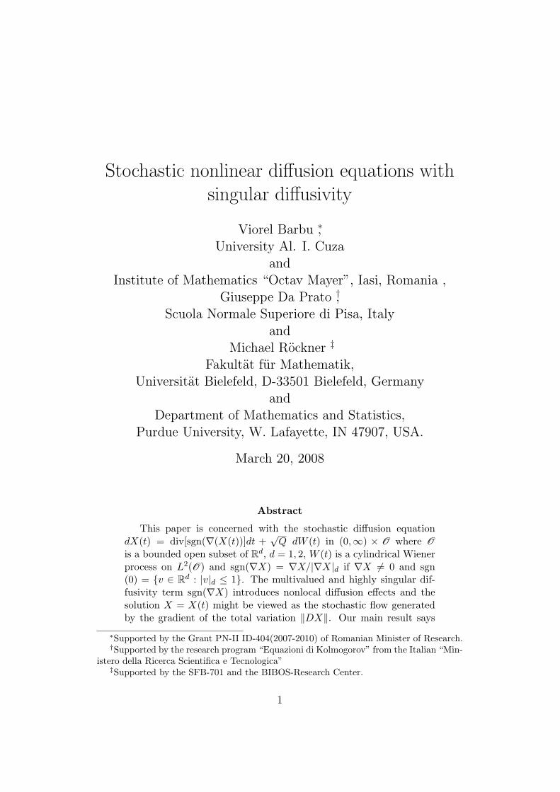
Stochastic nonlinear diffusion equations withsingular diffusivity

Viorel Barbu ∗,University Al. I. Cuza

andInstitute of Mathematics “Octav Mayer”, Iasi, Romania ,

Giuseppe Da Prato †,Scuola Normale Superiore di Pisa, Italy

andMichael Rockner ‡

Fakultat fur Mathematik,Universitat Bielefeld, D-33501 Bielefeld, Germany

andDepartment of Mathematics and Statistics,

Purdue University, W. Lafayette, IN 47907, USA.

March 20, 2008

Abstract

This paper is concerned with the stochastic diffusion equationdX(t) = div[sgn(∇(X(t))]dt +

√Q dW (t) in (0,∞) × O where O

is a bounded open subset of Rd, d = 1, 2, W (t) is a cylindrical Wienerprocess on L2(O) and sgn(∇X) = ∇X/|∇X|d if ∇X 6= 0 and sgn(0) = v ∈ Rd : |v|d ≤ 1. The multivalued and highly singular dif-fusivity term sgn(∇X) introduces nonlocal diffusion effects and thesolution X = X(t) might be viewed as the stochastic flow generatedby the gradient of the total variation ‖DX‖. Our main result says

∗Supported by the Grant PN-II ID-404(2007-2010) of Romanian Minister of Research.†Supported by the research program “Equazioni di Kolmogorov” from the Italian “Min-

istero della Ricerca Scientifica e Tecnologica”‡Supported by the SFB-701 and the BIBOS-Research Center.

1

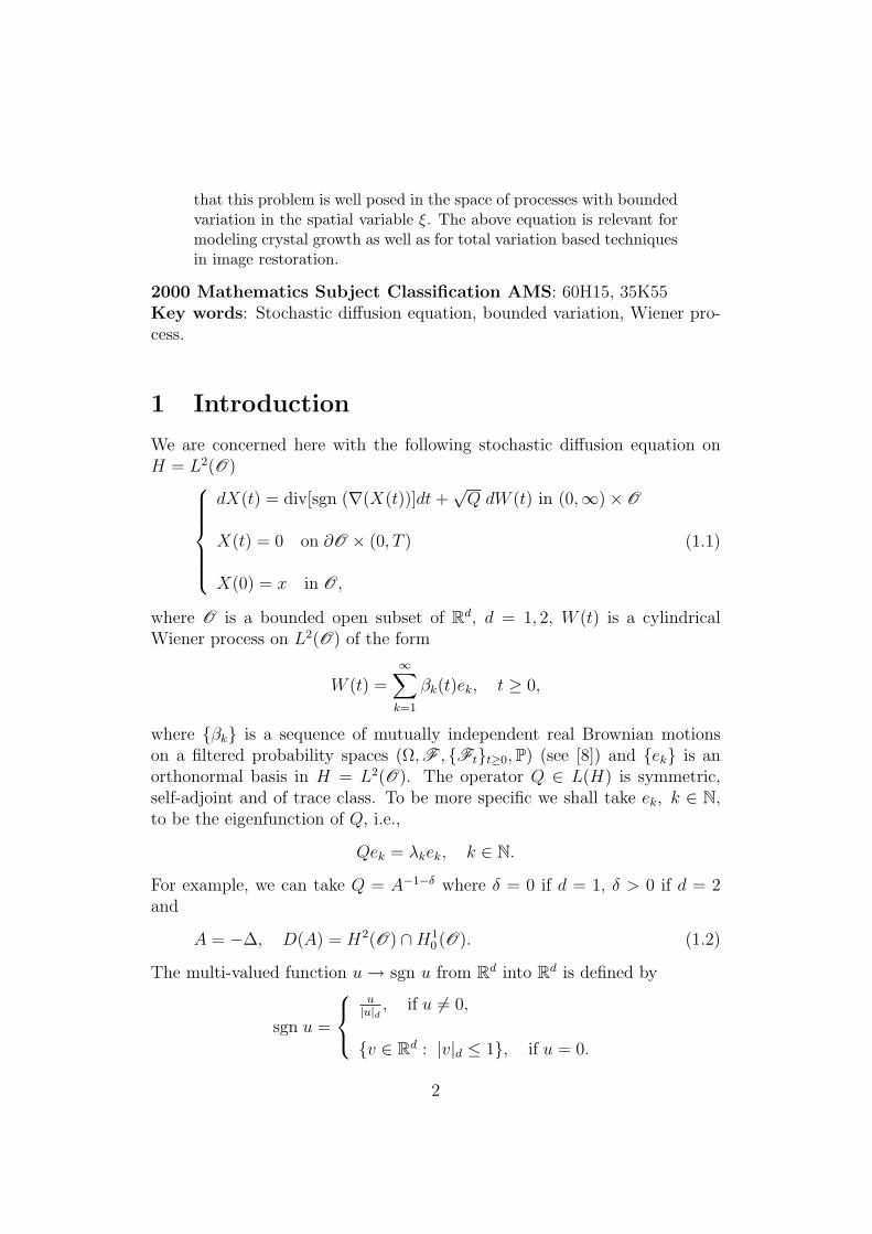
that this problem is well posed in the space of processes with boundedvariation in the spatial variable ξ. The above equation is relevant formodeling crystal growth as well as for total variation based techniquesin image restoration.

2000 Mathematics Subject Classification AMS: 60H15, 35K55Key words: Stochastic diffusion equation, bounded variation, Wiener pro-cess.

1 Introduction

We are concerned here with the following stochastic diffusion equation onH = L2(O)

dX(t) = div[sgn (∇(X(t))]dt+√Q dW (t) in (0,∞)× O

X(t) = 0 on ∂O × (0, T )

X(0) = x in O,

(1.1)

where O is a bounded open subset of Rd, d = 1, 2, W (t) is a cylindricalWiener process on L2(O) of the form

W (t) =∞∑k=1

βk(t)ek, t ≥ 0,

where βk is a sequence of mutually independent real Brownian motionson a filtered probability spaces (Ω,F , Ftt≥0,P) (see [8]) and ek is anorthonormal basis in H = L2(O). The operator Q ∈ L(H) is symmetric,self-adjoint and of trace class. To be more specific we shall take ek, k ∈ N,to be the eigenfunction of Q, i.e.,

Qek = λkek, k ∈ N.

For example, we can take Q = A−1−δ where δ = 0 if d = 1, δ > 0 if d = 2and

A = −∆, D(A) = H2(O) ∩H10 (O). (1.2)

The multi-valued function u→ sgn u from Rd into Rd is defined by

sgn u =

u|u|d, if u 6= 0,

v ∈ Rd : |v|d ≤ 1, if u = 0.

2

(Here | · |d is the Euclidean norm and 〈·, ·〉d is the Euclidean inner product.)Equation (1.1) is relevant in material science to describe the motion of

grain boundaries and in image processing. The first model is concerned withfaced growth of cristals derived from spatially homogeneous energy

E(X) =

∫O

|∇X|d dξ,

which formally leads to the gradient system

dX(t) = −div

(∇X(t)

|∇X(t)|d

)dt, t ≥ 0, (1.3)

or to (1.1) in presence of the Gaussian perturbation√Q dW . (We refer

to [11], [12], [17] for the presentation and treatment of the correspondingdeterministic models.)

The total variation based image restoration model based on E(X) hasbeen proposed in [19] (see also [7], [8], [16], [17]), i.e., as the solution to theminimization problem,

min

∫O

(|∇X|d +

1

2|X − f |2

)dξ, (1.4)

where f is the given image and X is the restored image. The minimizationproblem (1.4) leads to a flow X = X(t) generated by the evolution equation

dX(t) = −div

(∇X(t)

|∇X(t)|d

)dt− (X(t)− f(t))dt, t ≥ 0, (1.5)

which perturbed by a Gaussian process leads to equation (1.1). This restora-tion model was designed with the explicit aim to preserve edges and sharpdiscontinuities of the image.

In both equations (1.4) and (1.5) the discontinuous map u→ u|u|d

shouldbe replaced of course by its multi-valued maximal monotone graph u→ signu obtained by filling the jumps. It should also be mentioned that equation(1.1) (as well as the deterministic version (1.4) or (1.5)) is highly nonlinearand so the diffusion effect is non local. For instance in 1-D equation (1.1)has the form

dX(t) = −δ(∇X(t))∆X(t)dt =√Q dW (t), t ≥ 0, (1.6)

where δ is the Dirac measure at zero on O. Of course this is only a formalrepresentation because the multiplier δ(∇X(t)) is not well defined and so(1.6) does not make sense.

3

The main result established here (see Theorem 3.2 below) is concerned,however, with existence and uniqueness of a variational solution for d = 1, 2in the space of functions with bounded variation in the spatial variable ξ ∈O. A similar result is proved in Section 6 for equation (1.1) with linearmultiplicative noise along with positivity of solutions.

It should be noted that, though equation (1.1) arises in a variational set-ting, its existence theory is not covered by the classical results of E. Pardoux[14] or N. Krylov and B. Rozovskii [13] (see also [15], [18]). Indeed a generalstochastic equation of the form

dX(t) = div (a(∇(X(t)))dt+√Q dW (t) in (0,∞)× O

X(t) = 0 on ∂O × (0, T )X(0) = x in O,

(1.7)

where a : Rd → Rd is a monotonically increasing, continuous and coercivevector field with polynomial growth can be solved in the abstract variationalsetting

dX(t) + AX(t)dt =√Q dW (t)

X(0) = x(1.8)

where A : V → V ′ is a nonlinear monotone and demi-continuous operator(see [2]) such that

(Ax, x) ≥ ω‖x‖pV − ω1|x|2H ,

‖Ax‖V ′ ≤ C1‖x‖p′

V + C2,1

p+

1

p′= 1.

(Here V ⊂ H ⊂ V ′ is a classical variational Gelfand triple.)This is exactly the variational stochastic framework developed in [14],

[13], which however does not apply in this situation. As a matter of fact, thesituation considered here is a limit case of (1.7)-(1.8) and this fact will beexploited later to obtain existence of solutions for (1.1).

Notations. Everywhere in the following H is the Hilbert space L2(O)with the scalar product (·, ·) and the norm | · |). Lp(O), p ≥ 1, and V =H1

0 (O), V ′ = H−1(O) are the standard spaces of integrable functions andSobolev spaces on O. By CW ([0, T ];H) we shall denote the space of allcontinuous functions from [0, T ] to L2(Ω;H) which are adapted to W . Thespaces L2

W (0, T ;V ) and L2W (0, T ;V ′) are similarly defined. We shall denote

by ‖ · ‖ the norm of V , and spatial variables in O are denoted by ξ.

4

Existence of strong solutions for stochasticporous media equation under general

monotonicity conditions

Viorel Barbu ∗,University Al. I. Cuza

andInstitute of Mathematics “Octav Mayer”, Iasi, Romania ,

Giuseppe Da Prato †,Scuola Normale Superiore di Pisa, Italy

andMichael Rockner ‡

Faculty of Mathematics, University of Bielefeld, Germanyand

Department of Mathematics and Statistics, Purdue University,U. S. A.

February 5, 2008

Abstract

This paper addresses existence and uniqueness of strong solutionsto stochastic porous media equations dX −∆Ψ(X)dt = B(X)dW (t)in bounded domains of Rd with Dirichlet boundary conditions. HereΨ is a maximal monotone graph in R×R (possibly multivalued) with

∗Supported by PN-II ID.404 (2007-2010).†Supported by the research program “Equazioni di Kolmogorov” from the Italian “Min-

istero della Ricerca Scientifica e Tecnologica”‡Supported by the SFB-701 and the BIBOS-Research Center.

1

the domain and range all of R. Compared with the existing literatureon stochastic porous media equations no growth condition on Ψ isassumed and the diffusion coefficient Ψ might be multivalued anddiscontinuous. The latter case is encountered in stochastic models forself-organized criticality or phase transition.

AMS subject Classification 2000: 76S05, 60H15.Key words: stochastic porous media equation, Wiener process, convex

functions, Ito’s formula.

1 Introduction

This work is concerned with existence and uniqueness of solutions to stochas-tic porous media equations

dX(t)−∆Ψ(X(t))dt = B(X(t))dW (t) in (0, T )× O := QT ,Ψ(X(t)) = 0 on (0, T )× ∂O := ΣT ,X(0) = x in O,

(1.1)

where O is an open, bounded domain of Rd, d ≥ 1, with smooth boundary∂O, W (t) is a cylindrical Wiener process on L2(O), while B is a Lipschitzcontinuous operator from H := H−1(O) to the space of Hilbert–Schmidtoperators on L2(O). (See Hypothesis H2 below).

The function Ψ : R → R (or more generally the multivalued functionΨ : R → 2R) is a maximal monotone graph in R× R. (See the definition inSection 1.1 below).

Existence results for equation (1.1) were obtained in [8] (see also [3],[4])in the special case B =

√Q, with Q linear nonnegative, Tr Q < +∞ and

Ψ ∈ C1(R) satifying the growth condition

k3 + k1|s|r−1 ≤ Ψ′(s) ≤ k2(1 + |s|r−1), s ∈ R, (1.2)

where k1, k2 > 0, k3 ∈ R, r > 1.Under these growth conditions on Ψ, equation (1.1) covers many impor-

tant models describing the dynamics of an ideal gas in a porous medium(see e.g. [1]) but excludes, however, other significant physical models such asplasma fast diffusion ([5]) which arises for Ψ(s) =

√s and phase transitions

or dynamics of saturated underground water flows (Richard’s equation). In

2

the later case multivalued monotone graphs Ψ might appear as in [12]. Re-cently in [15] (see also [14]) the existence results of [8] were extended to thecase of monotone nonlinearities Ψ such that s 7→ sΨ(s) is (comparable to) a∆2-regular Young function (cf. assumption (A1) in [15]) thus including thefast diffusion model. As a matter of fact, in the line of the classical work ofN. Krylov and B. Rozovskii [10] the approach used in [15] is a variational onei.e. one considers the stochastic equation (1.1) in a duality setting inducedby a functional triplet V ⊂ H ⊂ V ′ and this requires to find appropriatespaces V and H. This was done in [15] in an elaborate way even with Ounbounded and with ∆ replaced by very general (not necessarily differential)operators L.

The method we use here is quite different and essentially an L1-approachrelying on weak compacteness techniques in L1(QT ) via the Dunford-Pettistheorem which involve minimal growth assumptions on Ψ. Restricted to sin-gle valued continuous functions Ψ the main result, Theorem 2.2 below, givesexistence and uniqueness of solutions only assuming that lims→+∞Ψ(s) =+∞, lims→−∞Ψ(s) = −∞, Ψ monotonically increasing and

lim sup|s|→+∞

∫ −s0

Ψ(t)dt∫ s0

Ψ(t)dt< +∞. (1.3)

We note that the assumptions on Ψ in [15]) imply our assumptions. In thissense, under assumption (H2) below on the noise, the results on this paperextend those in [15] in case L = ∆ if O is bounded and if the coefficients donot depend on (t, ω). The latter two were not assumed in [15]. On the otherhand a growth condition on Ψ is imposed in [15] (cf. [15, Lemma 3.2]) whichis not done here. Another main progress of this paper is that Ψ is no longerassumed to be continuous, it might be multivalued and with exponentialgrowth to ±∞ (for instance of the form exp (a|x|p)). We note that (1.3) isnot a growth condition at +∞ but a kind of symmetry condition about thebehaviour of Ψ at ±∞. If Ψ is a maximal monotone graph with potential j(i.e. Ψ = ∂j) then (1.3) takes the form (see Hypothesis (H3) below)

lim sup|s|→+∞

j(−s)j(s)

< +∞.

Anyway this condition is automatically satisfied for even monotonically in-creasing functions Ψ or e.g. if a condition of the form (1.2) is satisfied. We

3

note, however, that because of our very general conditions on Ψ the solu-tion of (1.1) will be pathwise only weakly continuous in H. The question ofpathwise strong continuity of solutions, however, remains open. The mainreason is the absence of a variational setting for problem (1.1) (see [10],[14])in the present situation. Other major technical difficulties encountered herein the proofs are that e.g. the integration by parts formula or Ito’s formula(see Lemmas 3.1 and 3.2 below) cannot be applied directly because of thesame reason. It should be said, however, that the L1 approach used here,which allows to treat very general nonlinearities, is applicable to determin-istic equations as well and seems to be new also in that context. On theother hand, the existence for the deterministic part of equation (1.1) is animmediate consequence of the Crandall–Liggett generation theorem for non-linear semigroups of contractions (see [2]) which is, however, not applicableto stochastic equations.

1.1 Notations

O is a bounded open subset of Rd, d ≥ 1, with smooth boundary ∂O. Weset

QT = (0, T )× O, ΣT = (0, T )× ∂O.

Lp(O), Lp(QT ), p ≥ 1, are standard Lp- function spaces and H10 (O), Hk(O)

are Sobolev spaces on O. By H := H−1(O) we denote the dual of H10 (O)

with the norm and the scalar product given by

|u|−1 := (A−1u, u)1/2, 〈u, v〉−1 = (A−1u, v),

respectively, where (·, ·) is the pairing between H10 (O) and H−1

0 and thescalar product of L2(O). Here A denotes the Laplace operator with Dirichlethomogeneous boundary conditions, i.e.

Au = −∆u, u ∈ D(A) = H2(O) ∩H10 (O). (1.4)

Given a Hilbert space U , the norm of U will be denoted by | · |U and thescalar product by (·, ·)U . By C([0, T ];U) we shall denote the space of U -valued continuous functions on [0, T ] and by Cw([0, T ];U) the space of weaklycontinuous functions from [0, T ] to U .

Given two Hilbert spaces U and V we shall denote the space of linearcontinuous operators from U to V by L(U, V ) and the space of Hilbert-

4

! " #$&%'"( *)+,-.0/12 -,346578,579;:<

=">@?ACBEDGFH>JIK>@ACBELMONCPRQBS LNUTVBWTVXTVD"M@YIK>ZTVQDG[>ZTVBEP>@F(\;TR>ZTVBENUTVBEPGN>@L]_^``FEBEDG]KIK>ZTVQDG[>ZTVBEPGNGa

b7>@FED>dcfeg\#DG`TVDG[1?ACBEDJcfea8hi@hj#cOc"k'XPRQ8>@ACDGNUTamlMO[>@LBH>ano [>@BEF,prqO[>@ACBELM;st>@P>@]&u ACMaq>@?BE[>@ACBELMONCPRQBvsw>@QM#Mu PGMO[

x(yZz|,!~C& zr,fZzCzr. 'z|,Zf.@U f 6z f Zz,W~z| Zz "CGZ~R Zz " C~rC ,U,zU& !z|C z|,UZ~7@U f z f ,~ G,U,7C ~R,,y U,Cz|,!~ G,~7@U f¡ z&,RC~Z U ,Cz z ,UZfC¢y"@U f |t,"~ 7,C~8zZ~ & ~,G~ £ f Cz~~, ~R,(~,V ~R ,y U* Gzr@U f (z f zm,RC ~t~¤ fC¢@ G U,U.¥( C7Z~,Cz,z,Cz !z~Z¦~.Z~z,z,t ,C GUZz, & z|,UZ@~(C~z f ,r Z~G,y U.§(ZfU Zz fU,C @ CzCz z z6 G"§( GUCz,z6U~¦y@yf!~ C rU~z&;~ yZ~ 6¨ Zz, ,©rC Z ;f Z~R,C z7(zUZzy Zz |8ªCz !z@ z f ~z7f, (y@ ~V ~R«~ 7~,,R fC & 7Z~@U~«z Z ZfCz 7z|,Zf" 7f UU!~R,'U~z'ZfU @ Cz zr C £~yZzUZ & 7 z|,UZ6&~R C~z|~z f £ Cz,z, «~ ~. ~Rryf!~ C . Zf UU!~R,U~z z,RC~Z !zr~z7f, ry@ ~V z& z,Zz,zC & r U, U~O,Cz !z~, Zz|,!~R,C~R UZy7U U~~ U~R Zz,~6,C~O,y U¬&~R,U f¤Z ,!~R C~z «zU

­®G¯m°±V²³r²C²R´µR¶·&¸C¹´±UµC³º±´µR¶·rº¸´¶U¹V®¸V²»7¼½R¾m¿RÀ,ÁV °JÃÄCÅGÆ Ç ÅGÈÉÊËÉÊÉUÌfÄCÆ Ç Í"Î;ÏÐ;Ñ!´ÒÓEÉUÍ!Í,Ê|È,Ô|Ç ÕVÈ.ÄCËfÈ,ÊÉÔ|ÄUÊ|Ñ!´6ÎOÈ,Ê|Ç ÄÖÇ ÍtÑvÄCÆ ×Ô|Ç ÄCÅGÑ!´ØOÇ ÙÈÖ6ËfÄCÇ ÅRÔÔ|ÚGÈ!ÄUÊ|È!Û7´GÎOÄUÊ|ÄC×GÑÛÈÖÇ ÉÜ Ý;Þ'ßà8áâ"ã.äß8åá'Þæ ¦ z',O z|,UZ(@U f z f Zz z Cz| ~R,C¢6W~z| fz CGZ~R Zzm C z|,, C~ |7; Zz ç UG~Z¢C t,U, ZfZCz~Z~ «~y@ ~V C'è@C ¤@U~ ,Ur, 7y R £ Zz 1ç UG~Z" fU R~R 6m C tZ 1~R~¤Z ,7R~ 7 z f ;'é8~ «~, @ z Z£

ê

CGZ~R Zz;~ zCz z z, UZCz#~ZfCz, y@ m&~R,U f¤Z ,!~R 7 UZzmz,~R,!~R,CHZz,~R,!~R,C'z «z ~!~,U ©UC'y7z|,, 6 C~ ff!~ ,@U CzU8x(«zZG U y@~fCGZ~R,&7ffU fZ~ UzR~ Zzë ë R(z @,Zz&~R,U ~«z&~z&U #~z& U fz U~; Zz .,fCz,zCzU& 7ffU#Zz z|!z Zz .CGZ~R ~7C r,U,ì@íì@î'ï¦ð6ñòó íGô#õgöø÷Uù ó íGôú"û "üþý.ÿ

U,ü z~@Uy@ZfCzyZzÿf ~' CU zz7 y@Z~,æ z,y U ñ ò ó|ï í 4ÿ z(~'6 R~ CZ tf¤ZC.~z

ñ ò ó ô ñmó ô í ù ò õ ô! í" ó ê ô U, ñ ó|ï íô ÿ8,U,CzUG t Zz ç UGC z~£@Gz G ZzU7, U~ Z,C~z Z ;y R t~Rí í"

ñmó ô$#&%('&)*þ í" ñmó ô+,%7 .- )* ó0/ ô~Z 2134 ñmó ô+Kõ ó65 ôó zU.~«z ê7 ô & .Zz|!~G7R~ %¦z' ñ ~R' . 7)£,U,CzUG!z6~~, ~R,G Zz' ,UZz f g tZf UU!~R,U~zm U ñ z@Gz æ &f UU!~R,mU~z ó U ñ z ~R VôC y@& z,Zz,zC tzC 5 z ,UZz ;y@ ~ C8 ZzCGUG, Zf UU!~R,U~z ñ ò ~z ,@U Cz ó ô óñ ò ó ô ï¢ñ ò ó:9 ôô óï;:9 ô<#=% óï;:9 ô>&UU, :9@?¦ó|ï íAó ôþ 2134 ñ ò ó ôþù ò ó ô& 2BCD ñ ò ó ô+ ï,Eæ ~y@R,U«~R Zz Zz+%Fír~Zù ò ~,@Gz R.Zz|!~G!zUæ zZ~@U~ R ~z,z7f ZztùHGVùI:JKIMLON2P Q Q Q P

ùI )*í )*,ù I AùI ó )GôRS)*ùI ó íôRþù I 'T)*~ZC~ 7@UG z(G Zz )*í EU ,URUC~z,z7 ~RrC~ ùI z( U,UG ~y )*íô!f z 7 W~& ~RrùI z& fU~ ¨ Zz, ,© f U, z|!zWVYXO'T)7zZ ~R

ó [Z ô\ ùI ó ô ï ùI ó ô]\ - VYX*\ ï \ ~ ^? )*í"X[ í"X í_ ê E E E M` E& z @ Cz z Z ZfCz~«z 'z ,Z~R " U¢z76ùI ~V 'fU R~R Cz&y R t~R& (íC 2134 ù 9I ó ôKõ óa ôb ,UZ.C~ ùI~R rR)~Z 8íryG |y Zz|!~GR~ Cz

/

ùI ó ô+,)' - ) ó0c ôùI ó ôþù I #í E ó6d ôb ~z,z7( ~Rm CU zz7 y@Z~, z7@GzC|' ze| GZ~!z$fhg~ZifOjZzZ ~RkfhglifOj(nm E& CGZ~R ¦ my@z|,Z C1 y@Z~,¢Z Zz ë f ¦~Z¦ªy |@ ¦«~R,U" ~!~,U © ~ R~ ~y 1@U,7C~y |þ' ¦y@Z~,nfOjZ~7U ó ù ó íGô ï ö ñòó íGôô8÷oúqp rfhgý.ÿó ù ó íGô ï ö ñ ò ó íGôô8÷o ïYs#ñ ò ó íGô&útû qfOj.ý.ÿ U, s fOj sOt svu z(~7G Zz&@Gz Z ; sOt 'T) E& ¤ZZ~#~ z&, Cz| ~R,r z|,UZ~Z,@U Cz& 7@U f z f ZzU

í ów ¡ôRdí ów î#õ¦¡ô~ wr? ü~ 8î ? ÿf¡H'&)*ZfU ~z,z7f ¦ ¡ ï @U f |¢& ,y U Z~!~7,U!zU8ûFhp~Z.û E& ' z|,UZ6 7z f Zz(, Zz 'CGZ~R Zzr&~z(,,C~R,Ct R~ Zz,C GCzry.~.~f !zr~Zt' ,'~7 U!z ',fzx6@y'x(,Zz ó zU / ô*zZ 8 ~ ó zU H ê )"ô*|( 8 ~z,z ~ZzZ ¨~~©CGU© ó zU êê ôG~(, ó zU ê ô b x( ~ZèO¨;Z! ~Zz ó ê ôé v(U «~6~E c H d H b 7UG ~R~'z@C ~O~R,UG ~zmy@UU.fU,C7,'R~ Zzm~z@C!z Zz ¢,y UzyzZ;¨~©CGU©7~Z£7 , U,z76 , Cz, z ,UZfC, z&, / ê H // HZ~Z 7 !~ /:a H æ y@ /5 «~ 7y@ ~V ó .@U f Côz f Zz, C~( Zz tCGZ~R Zz z& fU ,CzUG,C8x(«zZ U,~, Z ZfCUKG, yf Zz,U«~R,C, Z t U7UZ~7 6z f Zz(W~z| Zz tCGZ~R ZzU 8 ZU, ,U!~R,,7 Zz U "fC U~R,C£,. z|,Zf£@U f z f Zz,"éx| ,r G Z~@U ê c ~Z r7 !~ z ê 5 ~Z ê / O U,z7ryZ~z Uz,Cz !z&.z f @U f |~,,CzUG,Cæ . ,CzUGr, ~R U~R U~,,C~R,7UGr ,y U W~z| Zz ¢ ~ " C~C ",U, zfUU @C £ 7!~7U,O r U,'U f CGZ~R Zz Ò v~U, C~6 R~ CfU!~R,!z Y y@UzZ~CzUù yZ~ t¨ Zz, ,© z|,UZ GUCz,z~ZR~ Zz,@U Czm; z f Zz,' C~& Zz 7ffU«zmU,z|,Z C ê d H ê: ó W~z|( Zz 7ffU ô~Z a ó z@U! Zz 7ffU ô& z|,Zf,U!z,(y@ mZf UU!~R,m~Zf UU!~R,z ,Z~R Zz#,U«~R,C, @U!~R,(~ . 6CGZ~R ;&x( y@ Z z|,UZ #y@z|,Z C£ G,U,7C ~R,,y U ,Cz|,!~ G,"~@U f¢¡¬~Z" UC# ,Cz ; y@ ,UZfCyr@U f |r,(~ 7,C~zZ~ æ Zf UU!~R,U~zG ~,G~ r z|,Zf# z|,UZ~'@U f z f ,~~, ~R,&~,V ~R ,y U ~Z z8 y@(f ~~r¤ fC'@ G U,U.¥( C@7Z~,Cz,z&,Cz !z~Z.~7Z~z,z,7 (,C G ; C~

5

, z|,UZr#~C~7z f , Z~Z,y U.(RUUCZfU Zz fU,C @ CzCz z f Oy@r& G8x_Z~m; r,Wzm ,CG ,,Cz !z6J . z|,UZ( tz f Zz,1U!~ ~yZz|,!~',y Uz . ~Vy@UU.yf!~ C(z , U,UG7ffU«z ê7 ~Z U, ;y@,,Cz@Z ,Cxr Z~8,@U Czr '@U f 'z f ZzU~£y@'yf!~ C " U~z~ yZ~ g¨ Zz, ,©.,!~Zz@7,U,. & Cz Z Zft t GUCz,z @U f z f .~Z.~7U!~ .~z7f, y@ ~V Cæ f UU!~R,U~z C (,U,z ~ O,R( z|,UZ~R C~z|6~@U f z f ; & 7¤ZZ~8Z~m ~ 7 y@ZU,C z77,Cz !zfZz £ f UU!~R,7z f 1~z7f, 7y@ ~V ~R«~ 7 & zrZ~r y@7fUU @C ",U«~R t U,.ZU, yZ~y@ ~V ( 'z f Zz&, C~(U f .CGZ~R Zz,CzUG,C ê / H& ' U, U~,Cz !z y@ Zz|,!~R,C¢~R 7UZ£yt7U U~8~ U~R Zz,~',C~O,y U &~R,U f¤Z ,!~R . C~z «zU

qÞ.á'Þ.ârW.rÞq(àßvä$O& zU~z Czm Z Zz ñ ñ ò z@C ¤@,@U Cz ó0/ ô&~Z ó ô< ,@hkOnk* R¡¢h

æ t 7zyZzCGUGZ~r'z ~ fU,6y.¡ø~@Gz 66y@UCO~,y ,!~,yf¤ fC& zzyZzC zfU,Ct, Cz| ~R "m z|,UZ'@U f z f Zz,' 7ffU;7UG Cy@,yf(~6 7@U f¡W

ì@íì@î'ï¦ð6ñ ò ó íGô#õgöø÷Uù ó íGô&útû £¤þü_ý ó )*¡ô! ó ôó ù ó íGô ï ö ñòó íGôô8÷oúqp ¥+gSfhgý ó )*¡ô! ó 7 ô

ó ù ó íGô ï ö ñ ò ó íGôô÷"o ïYs#ñ ò ó íGô&ú"û ¥<j,fOj.ý ó )*¡ô! ó ôí ów M)Gô í ów ¡ô "ü E ó ê )Gôb z ~ ,Rr ,Cz !z&ZfU ~z,z7f Zz ó ôH ó ô ó0/ ôH óa ô&~Z ó [Z ô E¦h§O¨O©ª«6¬F¨O­*®¯0°:­*±³²´.¬°"µ z,~rz 7 |z ~ fU, z,U~«~,ffZ7~Z1 , &¶> ó üôy ó ÷ U÷ ô~Zn·R÷¸·O,Cz@C U x(«zZ8z ~ . U , ¢ G, !~Zzr Z ¦~ 7UG!z ,U,CzUG G, !~R R~ ~y CzU& (,y U Zy@,,C~R,C7 7 Z Z~!~7U,,U,CzUG,C6y¹ ,º N ó üô& . !zfZ~ ¹ 9 ó º N ó üôô 9 E & , ¹ z(f¤ZCy·2»·¼½¾F¿~À\ ö.»\ > w õ&¿Á sów ô@\ »\ > ÃÅÄ NÆ > ó êê ô

a

CONVERGENCE OF THE FINITE DIFFERENCE SCHEME FORA FASTDIFFUSION EQUATION IN POROUS MEDIA

Cornelia Ciutureanu, Institute of Mathematical Statistics and Applied Math-ematics, Bucharest, Romania

Gabriela Marinoschi1 , Institute of Mathematical Statistics and Applied Math-ematics, Bucharest, Romania

Keywords Boundary value problems for nonlinear parabolic PDE; PDEwith multivalued right-hand sides; Free boundary problems for PDE; Stabilityand convergence of numerical methods; Flows in porous media.

AMS Subject Classication 35K60; 35R70; 35R35; 65M12; 76S05.

Abstract.We are concerned with an implicit scheme for the nite di¤erence solution

to a nonlinear parabolic equation with a multivalued coe¢ cient which describesthe fast di¤usion in a porous medium. The boundary conditions contain themultivalued function as well. We prove the stability and the convergence of thescheme, emphasizing the precise nature of convergence in this specic case andcompute the error level of the approximating solution. The method is aimed tosimplify the numerical computations for the solutions to equations of this type,without performing an approximation of the multivalued function. The theoryis illustrated by numerical results.

1 Introduction

Apart from other di¤usion processes, the di¤usion of a uid in a porous medium,consisting in a solid matrix and a void part, has a specic behavior in relationwith the medium structure, specically with the pore geometry and the volumeof voids. Under certain conditions depending on the soil structure, the rate atwhich the uid may be supplied on a part of the domain boundary, the initialdistribution of the uid in the soil, the presence of underground sources andthe boundary permeability, a part or more of the ow domain may saturateand the pores in these regions become completely lled with the uid. In thesaturated part the uid concentration in the pores attains the maximum value,or the saturation value, which will be denoted in this paper by s: This is apositive number equal to the value of the medium porosity (assuming e.g., that

1Address correspondence to Gabriela Marinoschi, Institute of Mathematical Statisticsand Applied Mathematics, Calea 13 Septembrie 13, Bucharest, Romania; E-mail: gabi-marinoschi@yahoo.com, gmarino@acad.ro

1

it is constant) and it is specic to each material. At the interface between thesaturated and unsaturated parts a free boundary is formed and it may beginto advance towards the unsaturated part. In the model below its presence ischaracterized by a multivalued function.We consider an open bounded subset of RN (N 2 N = f1; 2; :::g); with

the boundary := @ piecewise smooth, composed by two disjoint parts uand : We denote the space variable by x := (x1; :::; xN ) 2 and the time byt 2 (0; T ); with T nite. We are concerned with the boundary value problemconsisting of a di¤usion equation with a transport term

@

@t() +r K() 3 f in Q := (0; T ) ; (1.1)

with the initial datum(0; x) = 0 in : (1.2)

Various boundary conditions on (0; T ) can be attached but we shall illus-trate the theory by considering nonhomogeneous Neumann and Robin boundaryconditions of the form

(K()r()) 3 u on u := (0; T ) u; (1.3)

(K()r()) () 3 f0 on := (0; T ) ; (1.4)

where is the normal vector to : The second condition expresses the fact thatthe boundary is semipermeable (with characterizing its variable permeabil-ity). The meaning of the equations (1.1)-(1.4) will be explained a little furtherin the denition of the solution.In this problem : R! R is a graph dened as

(r) :=

8<:R r0()d; if r < s;

[Ks ;+1); if r = s;

?; if r > s;(1.5)

where : (1; s) ! R is a positive, di¤erentiable, strictly monotonicallyincreasing function, which blows up at r = s, but having the integral nite atthis point. Namely we set

(r) > 0; for each r < s; (r) := for r 0; (1.6)

limr%s

(r) = +1, (1.7)

limr%s

Z r

0

()d = Ks : (1.8)

Consequently, has the properties

((r) (r)) (r r) (r r)2; for every r; r 2 (1; s]; (1.9)

limr!1

(r) = 1; (1.10)

2

limr%s

(r) = Ks : (1.11)

A particular case of this model was set up in [1] for describing the saturated-unsaturated water inltration in soils. The hypotheses (1.7)-(1.8) reveal thecharacter of fast di¤usion (see [2], [1]).We notice that ()1 : R!(1; s] ! is single-valued, monotonically

increasing on (1;Ks ) and constant for r 2 [K

s ;+1); i.e., ()1(r) = s:Also, by (1.9) it follows that ()1 is Lipschitz continuous on R with theconstant 1

:

The vector K(r) = (K1(r); :::;KN (r)) has each component nonnegative andbounded,

0 Ki(r) Ksi for any r 2 R: (1.12)

Moreover we consider that

Ki(r) = 0 for r 0 and Ki(r) = Ksi for r s: (1.13)

In the above relationships ; s;Ks and K

si are positive known constants

and we shall denoteKs = max

i=1;:::;NfKs

i g: (1.14)

We shall study the case in which Ki is Lipschitz, satisfying

jKi(r)Ki(r)j Mi jr rj for all i = 1; :::; N: (1.15)

Finally, we assume that : ! [m; M ] is a positive continuous function,i.e., m > 0:

1.1 Functional framework and preliminary results

For simplicity, we shall denote the scalar product and norm in L2() with nosubscript, i.e., by (; ) and kk ; respectively, and consider V = H1() with thenorm

k kV =Z

jr (x)j2 dx+Z

(x) j (x)j2 d1=2

; (1.16)

which is equivalent with the standard norm on the Hilbert space H1(): Indeed,there exist the positive constants denoted cH ; c ; cu depending on

1=2m ; the

domain and the dimension N; such that

k kH1() cH k kV ; k kL2() c k kV ; k kL2(u) cu k kV ;(1.17)

for any 2 V: These relationships are easily deduced via the trace theorem andPoincaré inequality (see [1], page 137).We endow the dual V 0 of V with the scalar product

(; )V 0 = h; iV 0;V ; for any ; 2 V 0; (1.18)

3

WELL-POSEDNESS FOR A HYPERBOLIC-PARABOLICCAUCHY PROBLEM ARISING IN

POPULATION DYNAMICS1

MIMMO IANNELLI

Mathematics Department, University of Trento, via Sommarive 14, 38050Povo (Trento), Italy, e-mail: iannelli@science.unitn.it

GABRIELA MARINOSCHI

Institute of Mathematical Statistics and Applied Mathematics, Calea 13Septembrie 13, 050711 Bucharest, Romania, e-mail: gmarino@acad.ro

Abstract. In some previous work [1]-[3], the authors have considered the dif-fusion of a population in a multilayered habitat, taking into account both thedemographic structure, due to the age distribution of the individuals, and thespatial distribution related to population spread and diffusion. The developmentof the mathematical framework for this kind of problems leads the attention ona linear problem which incorporates all the features that make this kind of prob-lems unusual. This model is represented by a system of PDE with discontinuouscoefficients and data and sources at the boundaries between layers with differentstructure. In this paper we provide well-posedness to such a problem together withregularity conditions, using m-accretiveness and fixed points techniques.

1 Introduction

The modelling of age-structured populations, spreading in a geographical region,leads to analyze non linear P.D.E. with non-local terms that are strictly related tohereditary effects such as those represented in the framework of integral equationsof Volterra type. In particular, in some previous work [1]-[3], the authors have con-sidered the diffusion of a population in a multilayered habitat, taking into accountboth the demographic structure, due to the age distribution of the individuals,and the spatial distribution related to population spread and diffusion.

1AMS Subject classification: 35K90, 35M10, 35R05, 92D25

1

However, the same problems studied in [1]-[3] lead to consider several techni-cal problems mainly focused on well-posedness of a certain linear system whichincorporates all the features that make this kind of problems unusual. Namelythe hyperbolic character with respect to the age variable (denoted by a ∈ [0, a+]),interacts with the parabolic features due to the spatial one (denoted by y ∈ [0, L]).The model is represented by a system of PDE with discontinuous coefficients anddata and sources at the boundaries between layers with different structure. Thus,in the present paper we provide a systematic approach to the problem, stating somebasic results in the framework that allows to treat various problems in populationdynamics such as the control problems approached in [3].

The same results may be of interest for other modelling problems with hyperbolic-parabolic behaviour and discontinuous coefficients and data.

We consider the domain Ω = (0, a+) × (y0, yn) composed of n parallel layers

Ωj = (0, a+) × (yj−1, yj), j = 1, 2, ...n,

and denoteΓyj

= (a, yj); a ∈ (0, a+), j = 0, ..., n,

where Γyjwith j = 0 and j = n are the exterior boundaries, while Γyj

withj = 1, . . . , n − 1 represent the interior ones. The time t runs within the finiteinterval (0, T ).

The model we are going to analyze reads

∂qj

∂t+∂qj

∂a−

∂

∂y

(Kj(a)

∂qj

∂y

)+ Tj(t)qj = fj

in (0, T ) × Ωj, j = 1, ..., n

qj(0, a, y) = q0j (a, y) in Ωj, j = 1, ..., n,

qj(t, 0, y) = Fj(t, y) in (0, T ) × (yj−1, yj), j = 1, ..., n,qj = qj+1 on (0, T ) × Γyj

, j = 1, ...n − 1,

Kj(a)∂qj

∂y= Kj+1(a)

∂qj+1

∂y+ kj(t, a)

on (0, T ) × Γyj, j = 1, ...n − 1,

−K1(a)∂q1

∂y= k0(t, a) on (0, T ) × Γy0

,

Kn(a)∂qn

∂y= kn(t, a) on (0, T ) × Γyn

,

(1.1)

assuming that

q0j ∈ L2(Ωj), fj ∈ L2(0, T ;L2(Ωj)), Fj ∈ L2(0, T ;L2(yj−1, yj)),

Tj ∈ C([0, T ];L(L2(Ωj), L2(Ωj)), kj ∈ L2(0, T ;L2(0, a+)),

Kj ∈ L∞(0, a+),Kj(a) ≥ K0 > 0 a.e. in (0, a+).

(1.2)

2

We introduce the generic notation defining the function Φ(t, a, y) in the set(0, T ) × Ω, by

Φ(t, a, y) = Φj(t, a, y), for y ∈ (yj−1, yj) (1.3)

where Φj stands for any function defined on (0, T ) × Ωj (see also the notations(25)-(32) from [1]). Vice-versa, if Φ is a function defined on (0, T ) × Ω, we defineΦj in (0, T ) × Ωj by setting

Φj(t, a, y) = Φ(a, t, y), y ∈ (yj−1, yj). (1.4)

Then, denoting

HΩ = L2(Ω), H = L2(0, L), V = H1(0, L),

with the standard norms, and using assumptions (1.2) we have

q0 ∈ HΩ, f ∈ L2(0, T ;HΩ), F ∈ L2(0, T ;H),

k ∈ L2(0, T ;L2(0, a+)), K ∈ L∞(0, a+).(1.5)

Moreover, we may define the operator T (t) : HΩ → HΩ setting

(T (t)θ)j = (Tj(t)θj),

where θ ∈ HΩ and we have used both (1.3) and (1.4). Then T (t) is continuous onHΩ, for each t ∈ [0, T ], and we have that

‖T (t)θ‖HΩ≤M ‖θ‖HΩ

,∀θ ∈ HΩ, M > 0. (1.6)

Concerning the previous problem we are lead to adopt the following definition:

Definition 1.1. A weak solution to problem (1.1) is a function

q ∈ C([0, T ];HΩ) ∩ L2(0, T ;L2(0, a+, V )) ∩ C([0, a+];L2(0, T ;H)) (1.7)

satisfying

−

∫ T

0

∫

Ωq∂ψ

∂tdydadt −

∫ T

0

⟨∂ψ

∂a(t), q(t)

⟩dt

+

∫

Ωq(T, a, y)ψ(T, a, y)dady +

∫ T

0

∫ L

0q(t, a+, y)ψ(t, a+, y)dydt

−

∫

Ωq0(a, y)ψ(0, a, y)dyda −

∫ T

0

∫ L

0F (t, y)ψ(t, 0, y)dydt

+

∫ T

0

∫

Ω

(K(a, y)

∂q

∂y

∂ψ

∂y+ (T (t)q(t)) (a, y)ψ(t, a, y)

)dydadt

=

∫ T

0

∫

Ωfψ dydadt +

∫ T

0

∫ a+

0

n∑

j=0

kj(t, a)ψ(t, a, yj)dadt,

(1.8)

3

for any function ψ such that

ψ ∈ L2(0, T ;L2(0, a+;V )) ∩W 1,2(0, T ;HΩ),

ψa ∈ L2(0, T ;L2(0, a+;V ′)).

(1.9)

We specify that 〈·, ·〉 denotes the duality between L2(0, a+;V ) and L2(0, a+;V ′)defined as

〈h, g〉 =

∫ a+

0〈h(a), g(a)〉V ′,V da, ∀h ∈ L2(0, a+;V ′), g ∈ L2(0, a+;V ),

where 〈·, ·〉V ′,V is the pairing between V ′ and V .The aim of this paper is to prove existence and uniqueness to (1.1). To this end

we will proceed by steps, considering different particular cases of the full problem.

2 The basic problem

To approach our problem we first introduce the linear operator

B0 : D(B0) ⊂ L2(0, a+;V ) → L2(0, a+;V ′)

on the domain

D(B0) = v ∈ L2(0, a+;V ); va ∈ L2(0, a+;V ′), v(0, y) = 0, (2.1)

where we note that the condition v(0, y) = 0 is meaningful because v ∈ D(B0)implies that v ∈ C([0, a+];H).

We define B0 by setting, for v ∈ D(B0)

〈(B0v)(a), ψ〉V ′,V = 〈va(a, ·), ψ〉V ′,V +

∫ L

0K(a, y)vy(a, y)ψy(y)dy, (2.2)

for a.e. a ∈ [0, a+] and any ψ ∈ V .Then we define the operator B : D(B) ⊂ HΩ → HΩ, by

Bv = B0v,

on the domainD(B) = v ∈ D(B0); Bv ∈ HΩ.

4

1

NONLINEAR FEEDBACK CONTROLLERS FOR THE NAVIER-STOKESEQUATIONS

Adriana-Ioana LefterFaculty of Mathematics, “Al.I.Cuza” University, Iasi, Romania;

“O.Mayer” Institute of Mathematics, Iasi, Romania.1

Abstract. In this paper we prove the feedback stabilization of the Navier-Stokesequations preserving the invariance of a given convex set. To this aim we first de-duce an existence theorem concerning weak solutions for the Navier-Stokes systemperturbed with a subdifferential.2000 Mathematics Subject Classification: 76D05, 76D03, 47H05, 47J05, 35B35.Keywords and phrases: Navier-Stokes equations, strong and weak solution, mono-tone operator, feedback controller, exponential stability.

Let T > 0 and let Ω ⊂ IRd, d = 2, 3 be an open and bounded domain, witha smooth boundary ∂Ω (of class C2, e.g.). Consider the controlled Navier-Stokesequations

∂y

∂t(x, t)− ν∆y(x, t) + (y(x, t) · ∇)y(x, t)

+∇p(x, t) = f0(x, t) + u0(x, t), (x, t) ∈ Q = Ω× (0, T ),

div y(x, t) = 0, (x, t) ∈ Q,

y(x, t) = 0, (x, t) ∈ Σ = ∂Ω× (0, T ),

y(x, 0) = y0(x), x ∈ Ω,

(1)

where y = (y1, y2, . . . , yd) is the velocity field, p is the scalar pressure, the densityof external forces is f0 = (f01, f02, . . . , f0d), the constant ν > 0 is the kinematicviscosity coefficient and u0 = (u01, u02, . . . , u0d) is a distributed control on Ω.

We intend to find feedback controllers which would insure the exponential sta-bilization of the Navier-Stokes equations in invariance conditions. To this aim, letΦ be an operator satisfying the following hypotheses:(h1) Φ = ∂ϕ, where ϕ : H → IR is a lower semicontinuous proper convex

function (hence Φ is a maximal monotone operator in H ×H);(h2) 0 ∈ D(Φ);(h3) there exist two constants γ ≥ 0, α ∈ (0, (1/ν)) such that

(Aw,Φλ(w)) ≥ −γ(1 + |w|2)− α|Φλ(w)|2, ∀λ > 0,∀w ∈ D(A), (2)

where A is the Stokes operator and Φλ : H → H is the Yosida approximation of Φ.In order to prove stability we need a global solution for the controlled problem.

The results we have previously proved for strong solutions say that in dimensiond = 3 we may get only local strong solutions. That is why a stability resultin the three dimensional case requires an existence theorem for weak solutions.We give such a result in Section 2. In Section 3 we state and prove exponentialstabilization theorems. The first example uses a feedback controller distributed onthe entire domain (§3.1) and the stability result is global. In the second examplethe feedback controller belongs to a finite dimensional space and it is distributedon a subdomain(§3.2); the stability result is local.

1MAILING ADRESS: Faculty of Mathematics, “Al.I.Cuza” University, Bd.Carol I nr.11,

700506, Iasi, Romania. FAX: +40 232 201160 E-MAIL: ilefter@uaic.ro

This work was supported by CNCSIS Grant PN II ID 404/2008.

1

On a unique continuation property related to the

boundary stabilization of magnetohydrodynamic

equations

Catalin-George Lefter∗

Abstract

We prove that the MHD system in space dimension 2 is exponentiallystabilizable with boundary controllers. This result relies on a unique con-tinuation property for the adjoint linearized MHD system,

2000 Mathematics Subject Classification: 93D15, 35Q35, 76W05, 35Q30,35Q60, 93B07.

Keywords and phrases: Magnetohydrodynamic equations, feedback sta-bilization, stream function, unique continuation

1 Introduction

This paper is concerned with a unique continuation result which is appliedto the study of the local exponential stabilization for the magnetohydro-dynamic (MHD) equations in space dimension 2, with boundary feedbackcontrollers. We reduce the study, by a usual procedure, to the case ofinternally distributed controllers with compact support. It is howevernecessary to have divergence free controllers in the second equation.

The method we use for the stabilization is to linearize the systemaround the stationary state and then construct a feedback controller stabi-lizing the linear system. Then we show that the same controller stabilizes,locally in a specified space, the nonlinear system.

The stabilization of the linearized system is obtained via a spectral de-composition of the elliptic part. Thus, we project the system on the stableand unstable subspaces corresponding to this decomposition. The unsta-ble subspace is finite dimensional and the corresponding projected systemis exactly controllable, as a consequence of the approximate controllabil-ity of the original linearized system; one may thus construct a feedbackstabilizing this finite dimensional linear system. The projected system onthe stable subspace is asymptotically stable and the feedback for the fi-nite dimensional system is stabilizing the initial linearized equations. Theapproximate controllability of the linearized system is a consequence ofthe unique continuation result we describe below:

Let Ω ⊂ R2 be a bounded, simply connected open set with C2 bound-ary ∂Ω and ω ⊂⊂ Ω an open subset of Ω. Let Q = Ω × (0,∞), Σ =

∗This work was supported by the Minister of Education research grant PN II ID 404/2007-2010

1

∂Ω × (0,∞), n is the unit exterior normal to ∂Ω. We consider in thepaper the following MHD controlled system:

∂y

∂t− ν∆y + (y · ∇)y − (B · ∇)B +∇(

1

2B2 + p) = f + χωu in Q,

∂B

∂t+ η curl curl B + (y · ∇)B − (B · ∇)y = g + χωv in Q,

∇ · y = 0, ∇ ·B = 0 in Q,

y = 0, B · n = 0, rot B = 0 on Σ

y(·, 0) = y0, B(·, 0) = B0 in Ω.(1)

The functions that appear in the system have the following physical mean-ing: y = (y1, y2)T : Ω×(0, T )→ R2 is the velocity field, p : Ω×(0, T )→ Ris the pressure, B = (B1, B2)T : Ω × (0, T ) → R2 is the magnetic fieldand f = (f1, f2)T : Ω → R2 represents the density of the exterior forces((· · ·)T means the matrix transpose). The coefficients ν, η are the positivekinematic viscosity and the magnetic resistivity coefficients. We denoteby

rot B =∂B2

∂x1− ∂B1

∂x2

the scalar version of the curl operator. We also note the formula curl curl B =−∆B+∇div B. So, knowing the fact that the solution B will remain di-vergence free, we may write −∆B instead of curl curl B but we will keepthe notation to keep in mind that the system models in fact phenomenain a 3 dimensional cylindrical body and the data depend only on x1, x2

variables.The functions u, v : ω × (0, T ) → R2 ,u, v ∈ U := L2(0, T ; (L2(ω))2)

are the controllers and χω : L2(ω)→ L2(Ω) is the operator extending thefunctions in L2(ω) with 0 to the whole Ω. Moreover, div v = 0 in ω andv · n = 0 on ∂ω, where n is the normal to the boundary of ω.

Let (y, B) be a stationary solution. Let ξ =

(ζC

)with ζ, C written

as colon vectors. Then, the dual of the linearized system is:

−ζt −∆ζ + (∇C)B − (∇ζ)y + (∇B)TC + (∇y)T ζ +∇π = 0 in Q,

−Ct −∆C + (∇ζ)B − (∇C)y − (∇B)T ζ − (∇y)TC +∇ρ = 0 in Q,

∇ · ζ = 0, ∇ · C = 0 in Q

ζ = 0, C · n = 0, rot C = 0 on Σ.(2)

The central result is the following unique continuation property:

ζ = 0, rot C = 0 in ω × (0, T )⇒ ζ = 0, C = 0 in Ω× (0, T ). (3)

2