Solution Manual

for Microeconomic Theory

王 苏 生

Department of Economics

Hong Kong University of Science and Technology

September 2006

© Hong Kong University of Science & Technology, 2006

Page 2 of 73

I expect many errors in my solutions. I did not spend effort in eliminating errors. Please

send me an email if you find an error.

1. Exercises for Chapter 1 Exercise 1.1. A farm produces yams Y using capital K , labor L , and land according to

the production technology described by:

1 1 13 3 3= 3 .Y K L

The firm faces prices ( , , , )p q w r for ( , , , ).Y K L

(a) Suppose that, in the short run, K and are fixed. Derive the short-run supply and profit

functions of the firm.

(b) Suppose that, in the long run, K and L are marketable but is fixed. Derive the long-

run supply and profit functions. If there were a market for land, how much would the firm

be willing to pay for one more unit of land (the internal price of land)?

(c) Suppose that, in the long run, all the factors ,K L and are marketable. Does this pro-

duction function exhibit diminishing, constant, or increasing returns to scale? Suppose

that competitive conditions ensure zero profits. Derive the long-run supply and demand

functions.

Answer: (a) The short-run profit is

13max = max 3 ( ) ,SR

L LpY wL p KL wLπ ≡ − −

implying

23( ) = ,p KL K w

−

implying

3122= ( ) ,pL K

w⎛ ⎞⎟⎜ ⎟⎜ ⎟⎜⎝ ⎠

implying

11 123 2= 3( ) = 3 ( ) ,py KL K

w⎛ ⎞⎟⎜ ⎟⎜ ⎟⎜⎝ ⎠

implying

3 12 2= 2 .SR p w Kπ

−

Page 3 of 73

(b) The Long-run profit is

13

,= max 3 ( )maxLR

K LpY wL qK p KL wL qKπ ≡ − − − −

The FOC's are:

2 23 3( ) = , ( ) = ,p KL K w p KL L q

− −

implying

= or = .w K wK Lq L q

Substituting this solution into the first FOC, we can solve for :L

3

2= ,pLqw

implying

3 2

2= , = 3 ,p pK Yq w qw

implying

3

= = .LR ppY wL qKqw

π − −

The internal price of land will then be

3

= .LR p

qwπ∂

∂

(c) By the definition, the production exhibits CRS. The Long-run cost function is

13

( , , , ) min

s.t. = 3( )

C q w r Y wL qK r

Y KL

≡ + +

Take 133( ) .wL qK r Y KLλ

⎡ ⎤⎢ ⎥≡ + + + −⎣ ⎦L Then the FOC's are

2 2 23 3 3( ) = , ( ) = , ( ) = ,KL K w KL L q KL KL rλ λ λ

− − −

implying

= , = ,w K wq L r L

which imply that = wK Lq

and = .w Lr

Substituting these into the constraint, we can solve

for L and then K and :

Page 4 of 73

11 133 3

2 2 2

1 1 1= , = , = ,3 3 3

qr wr qwL Y K Y Yw q r

⎛ ⎞⎛ ⎞ ⎛ ⎞⎟⎜⎟ ⎟⎜ ⎜⎟⎟ ⎟⎜⎜ ⎜⎟⎟ ⎟⎜ ⎜⎜ ⎟⎝ ⎠ ⎝ ⎠⎝ ⎠

implying

13( , , , ) = ( ) ,C q w r Y wqr Y

implying

13= max ( , , , ) = [ ( ) ] .pY C q w r Y p wqr Yπ − −

Competitive market ensures zero profit, which requires that

13= ( )p wqr

in the long run. This means that no matter how much the firm produces the profit is always

zero. Therefore, the output Y is indeterminate, meaning that the firm may produce any

amount.

Exercise 1.2. Show that “ ( ) = ( ), , > 1nf x f x xλ λ λ+∀ ∈ R ” implies

( ) = ( ), , > 0.nf x f x xλ λ λ+∀ ∈ R

Answer: For any ny +∈ R and 0 < < 1,t let x ty≡ and 1.t

λ ≡ We then have

1( ) = ( ) = ( ) = ( ).f y f x f x f tyt

λ λ

Therefore, ( ) = ( ), > 0, ,ntf y f ty t y +∀ ∈ R where the equality for 1t ≥ is already given.

Exercise 1.3. Use a Lagrange function to solve 1 2( , , )c w w y for the following problem:

1 21 2 1 1 2 2,

1 2

( , , ) min

s.t. = .x x

c w w y w x w x

x x yρ ρ ρ

≡ +

+

Answer: See Varian (2nd ed.) p.31-33, or Varian (3rd ed.) p.55-56.

Exercise 1.4. Use a graph to solve the cost function for the following problem:

1 21 2 1 1 2 2,

1 2

( , , ) min

s.t. .x x

c w w y w x w x

y ax bx

≡ +

= +

Answer: From Figure 1.1, we see that the minimum point is ( , 0)ya

or (0, )yb

depending on

the ratio of 1

2

.ww

Therefore, the cost is 1w ya

or 2 .w yb

That is,

1 21 2( , , ) = min , .w wc w w y y y

a b⎧ ⎫⎪ ⎪⎪ ⎪⎨ ⎬⎪ ⎪⎪ ⎪⎩ ⎭

Page 5 of 73

.cxwxw =+ 2211

ybxax =+ 21Isoquant

2x

1x/y a Figure 1.1. Cost Minimization with Linear Technology

Exercise 1.5. Find the cost function for the following problem:

1 21 2 1 1 2 2

,

1 2

( , , ) min

s.t. = min { , }.x x

c w w y w x w x

y ax bx

≡ +

Answer: Since the production is not differentiable, we cannot use FOC to solve the problem.

One way to do is to use a graph.

1x

2x

/y a

yb

( )y f x=

1 2ax bx=

Figure 1.2. Cost Minimization with Leontief Technology

From Figure 1.2, we see that the minimum point is ( , ).y ya b

Therefore, the cost function is:

1 21 2( , , ) = .w wc w w y y

a b⎛ ⎞⎟⎜ + ⎟⎜ ⎟⎜⎝ ⎠

Exercise 1.6. In the short run, assume 2x is fixed: 2 = .x k Find STC, FC, SVC, SAC, SAVC,

SAFC, SMC, LC, LAC, and LMC for the following problem:

1 21 2 1 1 2 2

,

11 2

( , , ) min

s.t. = .x x

a a

c w w y w x w x

y x x −

≡ +

Answer: See Varian, Example 2.16, p.55 and p.66.

Page 6 of 73

Exercise 1.7. Prove the first two properties of the cost function.

Answer: The cost function and the expenditure function in consumer theory are mathemati-

cally the same.

Exercise 1.8. Prove the three properties of the demand and supply functions in Proposition

1.10.

Answer: (1) Since ( , )p wπ is linearly homogeneous and since ( , )( , ) = ,i

i

p wx p ww

π∂−

∂ ( , )ix p w

is homogeneous of degree 0 in ( , ).p w Similarly for ( , ).y p w

(2) By Hotelling's lemma, we have

1

1 1 12

1

1

( , ) = 0.

n

n

n n n

n

y y yp w wx x xp w wD p w

x x xp w w

π

⎛ ⎞∂ ∂ ∂ ⎟⎜ ⎟⎜ ⎟⎜ ∂ ∂ ∂ ⎟⎜ ⎟⎜ ⎟⎟⎜ ⎟∂ ∂ ∂⎜ ⎟⎜− − − ⎟⎜ ⎟⎜ ⎟∂ ∂ ∂ ≥⎜ ⎟⎟⎜ ⎟⎜ ⎟⎜ ⎟⎜ ⎟⎜ ⎟⎜ ⎟∂ ∂ ∂ ⎟⎜ ⎟− − −⎜ ⎟⎜ ⎟⎜ ∂ ∂ ∂⎝ ⎠

This immediately implies

0, 0,i

i

xyp w

∂∂≥ − ≥

∂ ∂

which gives the second property.

(3) By the symmetry of the matrix 2 ( , ),D p wπ we immediately have

= .ji

j i

xxw w

∂∂∂ ∂

Exercise 1.9. Consider the factor demand system:

1 12 2

2 11 1 2 11 12 2 1 2 22 21

1 2

( , , ) = , ( , , ) = ,w wx w w y b b y x w w y b b yw w

⎡ ⎤ ⎡ ⎤⎛ ⎞ ⎛ ⎞⎢ ⎥ ⎢ ⎥⎟ ⎟⎜ ⎜⎢ ⎥ ⎢ ⎥⎟ ⎟+ +⎜ ⎜⎟ ⎟⎜ ⎜⎢ ⎥ ⎢ ⎥⎟ ⎟⎜ ⎜⎝ ⎠ ⎝ ⎠⎢ ⎥ ⎢ ⎥⎣ ⎦ ⎣ ⎦

where 11 12 21 22, , , > 0b b b b are parameters. Find the condition(s) on the parameters so that this

demand system is consistent with cost minimization. What is the cost function?

Answer: If the demand system is a solution of a cost minimization problem, then it must

satisfy the properties listed in Proposition 1.9. Property (1) in the proposition is obviously

satisfied. Property (2) requires symmetric cross-price effects, that is,

1 2

2 1

=x xw w

∂ ∂∂ ∂

Page 7 of 73

or

12 211 2 1 2

1 1= .2 2

y yb bw w w w

Therefore, 12 21= .b b With 12 21= ,b b the substitution matrix is

3 1 1 11 1 2 2 2 2

1 2 1 21 2

12 1 1 1 32 2 2 2 2 2

1 2 1 21 2

1 12 2= .

1 12 2

x xw w y w w yw w

bx x

w w y w w yw w

− − −

− − −

⎛ ⎞ ⎛ ⎞∂ ∂ ⎟⎜ ⎟⎜⎟ ⎟⎜ −⎜⎟ ⎟⎜ ⎜∂ ∂ ⎟ ⎟⎜ ⎜⎟ ⎟⎜ ⎟ ⎜ ⎟⎟⎜ ⎟⎜⎟∂ ∂ ⎟⎜ ⎜⎟ ⎟⎜ ⎜⎟ ⎟−⎜ ⎜⎟ ⎟⎜⎟⎜∂ ∂ ⎝ ⎠⎝ ⎠

We have

1

1

< 0,xw

∂∂

and

( )

3 1 1 11 1 2 2 2 2

1 2 1 21 2 2 2 2 1 1 1 1

12 12 2 1 1 21 1 1 32 2 2 2 2 2

1 2 1 21 2

1 112 2= = = 0.41 1

2 2

x xw w y w w yw w

b b y w w w wx x

w w y w w yw w

− − −

− − − −

− − −

∂ ∂−∂ ∂

−∂ ∂

−∂ ∂

Thus, the substitution matrix is negative semi-definite. Finally, property (4) is implied by the

fact that the substitution matrix is negative semi-definite. Therefore, to be consistent with cost

minimization, we need and only need condition: 12 21= .b b

Let 12 21= .b b b≡ Then the cost function is

1 2 1 1 2 2 1 11 2 22 1 2( , , ) = = [ 2 ] .c w w y w x w x w b w b b w w y+ + +

Exercise 1.10. Show that if G satisfies Assumptions 1.1 and 1.2 and ( ) 0 mx xϕ′ > , ∀ ∈ ,R

then ( ) ( )F y G yϕ≡ also satisfies Assumptions 1.1 and 1.2.

Answer: Since ( ) [ ( )] ( ) 0i iy yF y G y G yϕ′= > , Assumption 1.1 is satisfied. Since

i j i j i jy y y y y yF G G Gϕ ϕ′′ ′= + ,

we have

1 1

1 1 1 1 1 1 1 1 1 1 1

1 1 1

0 0n n

n n n

nn n n n nn n n n n

y y y y

y y y y y y y y y y y y y y

y yy y y y y y yy y y y y

F F G GF F F G G G G G G G

F F F G G G G G G G

ϕ ϕ

ϕ ϕ ϕ ϕ ϕ

ϕ ϕ ϕ ϕ ϕ

′ ′

′′ ′′ ′′ ′

′ ′′ ′′′ ′

+ += .

+ +

Multiply the first column of the right determinant by jyGϕ

ϕ

′′

′− and then add what you have got

to the jth column. This operation won’t affect the value of the determinant. Thus,

Page 8 of 73

1 11

1 1 1 1 1 11 11 1 1 1

1 11

1

0 00

0

n nn

n nn

n nn n n n n nnn n n

y y y yy y

ny y y y y yy y y yy y y y y

y y y yy y y y y yy yy y y

F F G GG GF F F G G GG G G

F F F G G GG G G

ϕ ϕ

ϕ ϕ ϕϕ

ϕ ϕ ϕ

′ ′

′′ ′ +⎛ ⎞′ ⎟⎜ ⎟⎜ ⎟⎜ ⎟⎝ ⎠

′ ′′

= = < ,

for any = 2,3, .n m… Therefore, F also satisfies Assumption 1.2.

Exercise 1.11. A firm buys inputs at levels 1x and 2x on competitive markets and uses them

to produce a level of output .y Its technology is such that the minimum cost of producing y

at input prices 1w and 2w is given by the cost function

1 2 1 1 2 2 1 2( , , ) = ,a bc w w y A w A w Aw w yβ+ +

where 1 2, , , , > 0A A A a b and 2β ≥ are constant parameters.

(a) What parameter condition does the homogeneity of this cost function imply?

(b) Derive the conditional demand functions 1 1 2( , , )x w w y and 2 1 2( , , ).x w w y Verify that the

cross price effects are symmetric for these demand functions.

(c) Show that the MC curve is upward sloping and that the AC curve is U-shaped (convex).

Answer: (a) By

1 2 1 1 2 2 1 2( , , ) = ,a b a bc w w y A w A w A w w yβλ λ λ λ λ ++ +

we immediately see that the linear homogeneity of cost function implies that = 1.a b+

(b) We have

1 11 1 2 1 1 2 2 1 2 2 1 2

1 2

( , , ) = = , ( , , ) = = .a b a bc cx w w y A aAw w y x w w y A bAw w yw w

β β− −∂ ∂+ +

∂ ∂

Then,

1 11 21 2

2 1

= = .a bx xabAw w yw w

β− −∂ ∂∂ ∂

(c) When the functions are differentiable, taking derivatives is often the easiest way to

find monotonicity and convexity.

1 21 2 1 2( ) = , ( ) = ( 1) > 0.a b a bc dMC y Aw w y MC y Aw w y

y dyβ ββ β β− −∂

≡ −∂

11 1 2 21 2( ) = ,a bA w A wAC y Aw w y

y yβ−+ +

21 1 2 21 22 2( ) = ( 1) ,a bA w A wd AC y A w w y

dy y yββ −− − + −

2

31 1 2 21 22 3 3

2 2( ) = ( 1)( 2) > 0.a bA w A wd AC y A w w ydy y y

ββ β −+ + − −

Page 9 of 73

Therefore, MC is upward sloping and AC is U-shaped.

Exercise 1.12. Given a function 1 2( , ) ,a b cc w y Aw w y≡ where , > 0,A c

(a) Under what conditions, is this function a cost function?

(b) If the production function that results in this cost function is homogeneous, what is the

degree of homogeneity for this production function?

Answer: (a) Using Proposition 1.5, increasingness in w implies

, 0.a b ≥ (1)

Linear homogeneity implies that

= 1.a b+ (2)

We have

1 11 2 1 2

1 2

= , = ,a b c a b cc caAw w y bAw w yw w

− −∂ ∂∂ ∂

and

2 1 1

1 2 1 21 1 2

1 2 1 2

( 1)= .

( 1)

a b c a b c

w a b c a b c

a a Aw w y abAw w yD c

abAw w y b b Aw w y

− − −

− − −

⎛ ⎞− ⎟⎜ ⎟⎜ ⎟⎜ ⎟⎜ −⎝ ⎠

This implies that, using (2),

2 2

2 21 2 1 22 2

1 2

= ( 1) , = ( 1) ,a b c a b cc ca a Aw w y b b Aw w yw w

− −∂ ∂− −

∂ ∂

and

2 2( 1) 2( 1) 21 2= (1 ) = 0.a b c

wD c A w w y ab a b− − − −

Then, concavity requires that

1, 1.a b≤ ≤ (3)

(b) By Proposition 1.4, the degree of homogeneity must be 1/ .c

2. Exercises for Chapter 2 Exercise 2.1. Show that strong monotonicity implies local nonsatiation but not vice versa.

Answer: Since in any neighborhood of ,x we can always find a point y such that x y≥ and

,x y≠ strong monotonicity thus implies local nonsatiation.

Page 10 of 73

Suppose the preferences are defined by 1 2 1 2( , ) min{ , }.u x x x x≡ It is easy to see that the

preferences satisfy local nonsatiation. But for two points = (0, 1)x and = (0, 0),y we have

x y≥ and x y≠ but .x y∼ That is, the preferences don't satisfy strong monotonicity.

Exercise 2.2. A consumer has a utility function 1 21 2

1 1( , ) = .u x xx x

− −

(a) Compute the ordinary demand functions.

(b) Show that the indirect utility function is ( )2

1 2 .p p I− +

(c) Compute the expenditure function.

(d) Compute the compensated demand functions.

Answer: The consumer's problem is

1 2

1 1 2 2

1 1( , ) = max

s t = .

v p Ix x

p x p x I

− −

. . +

Let 1 1 2 21 2

1 1 ( ).I p x p xx x

λ≡ − − + − −L The FOC's

1 22 21 2

1 1= , =p px x

λ λ

imply 21 2

1

= .px xp

Substituting this into the budget constraint will immediately give us

*2

2 1 2

= .Ixp p p+

By symmetry, we also have

*1

1 1 2

= .Ixp p p+

(b) Substituting the consumer's demands into the utility function will give us

2

1 1 2 2 1 2 1 2 1 2 1 22 ( )( , ) = = = .

p p p p p p p p p p p pv p I

I I I I+ + + + +

− − − −

(c) Let = ( , ),u v p e i.e.

2

1 2( )=

p pu

e+

−

which immediately gives us the expenditure function:

2

1 2( )( , ) = .

p pe p u

u+

−

Page 11 of 73

(d) Substituting ( , )e p u for I in the consumer's demand functions we get

2

1 2 1 2 21

1 1 2 1 1 2 1 1

( )( , ) 1( , ) = = = = 1 .( )

p p p p pe p ux p uup p p p p p u u p p

⎛ ⎞+ + ⎟⎜ ⎟⎜− − − + ⎟⎜ ⎟⎜ ⎟+ + ⎝ ⎠

By symmetry,

12

2

1( , ) = 1 .p

x p uu p

⎛ ⎞⎟⎜ ⎟⎜− + ⎟⎜ ⎟⎜ ⎟⎝ ⎠

Exercise 2.3. Let ( , )ix p I∗ be the consumer's demand for good .i The income elasticity of

demand for good i is defined as ( , ) .i

ii

x p IIex I

∗∂≡

∂ Show that, if all income elasticities are

constant and equal, they must all be one.

Answer: Using the adding-up condition

( , ) =i ip x p I I∗∑

we can take derivative w.r.t. I on both sides of the equation to get:

= 1,ii

xpI

∗∂∂∑

implying

1 = = .i i i i ii

i

p x x p xI eI x I I

∗ ∗ ∗

∗

∂∂∑ ∑

If 1 2= = = ,ne e e then

1 = =i ii i

p xe eI

∗

∑

that is, 1 2= = = = 1.ne e e

Exercise 2.4. Show that the cross-price effects for ordinary demand are symmetric iff all

goods have the same income elasticity: ( , )( , ) = .ji

j i

x p Ix p Ip p

∗∗ ∂∂∂ ∂

Answer: By Shephard's lemma,

2 2( , ) ( , )= = = .ji

j j i i j i

xx e p u e p up p p p p p

∂∂ ∂ ∂∂ ∂ ∂ ∂ ∂ ∂

(4)

By Slutsky equation,

= = = ,j i j ii i i i i ij i

j j j i j

x x x xx x x x x xIx ep p I p I x I p I

∗ ∗ ∗ ∗∗ ∗ ∗∗

∗

∂ ∂ ∂ ∂ ∂ ∂− − −

∂ ∂ ∂ ∂ ∂ ∂

Page 12 of 73

where ie is the income elasticity of demand for good .i Similarly,

= = = .j j j j i j j j i ji j

i i i j i

x x x x x x x x x xIx ep p I p I x I p I

∗ ∗ ∗ ∗ ∗ ∗ ∗∗

∗

∂ ∂ ∂ ∂ ∂ ∂− − −

∂ ∂ ∂ ∂ ∂ ∂

By (4) and the fact that = ,i je e then

= .ji

j i

xxp p

∗∗ ∂∂∂ ∂

Exercise 2.5. A consumer has expenditure function 1/41 2 1 2( , , ) = .be p p u p p u What is the value

of b ?

Answer: Since ( , )e p u is linearly homogeneous in ,p 3= .4

b

Exercise 2.6. Suppose that the consumer's utility function is linearly homogeneous. Show

that the consumer's demand functions have constant income elasticity equal to 1.

Answer: We can easily show that ( , ) = ( , ), > 0,v p I v p Iλ λ λ∀ given that fact that

( ) = ( ), > 0.u x u xλ λ λ∀ Then, ( , )piv p I is linearly homogeneous in ,I and ( , )Iv p I is homo-

geneous of degree 0 in .I By Roy's identity, we then have

( , ) ( , )

( , ) = = = ( , ).( , ) ( , )

p pi ii i

I I

v p I v p Ix p I x p I

v p I v p I

λ λλ λ

λ∗ ∗− −

Taking the derivative w.r.t. λ , we then have

( , ) = ( , ).i

ix p II x p I

Iλ∗

∗∂∂

Setting = 1,λ we then have

( , ) = 1.i

i

x p IIx I

∗

∗

∂∂

Exercise 2.7. Use the envelope theorem to show that the Lagrange multiplier associated with

the budget constraint is the marginal utility of income; that is, ( , ) .v p I

Iλ

∂=

∂

Answer: The problem is

( , ) = max ( )

s t = .x

v p I u x

p x I. . ⋅

The Lagrange function for this problem is

( , ) ( ) ( ).x u x I p xλ λ≡ + − ⋅L

We have

Page 13 of 73

,

( , ) = ( , ) = ( ) ( ).maxx

v p I x u x I p xλ

λ λ+ − ⋅L

Then by the Envelop Theorem,

( , ) = .v p I

Iλ

∂∂

Exercise 2.8. Suppose that the consumer's demand function for good i has constant income

elasticity .η Show that the demand function can be written as 0 0( , ) = ( , )( / ) .i ix p I x p I I I η∗ ∗

Answer: Given

( , ) =i

i

x p IIx I

η∗

∗

∂∂

for all ,I we have

= log = log .ii

i

dx dI d x d Ix I

η η∗

∗∗ ⇒ ⋅

Thus,

0 0

0 0log = log log ( , ) log ( , ) = (log log ).I I

i i iI Id x d I x p I x p I I Iη η∗ ∗ ∗⇒ − −∫ ∫

Therefore,

00

( , ) = ( , ) .i iIx p I x p II

η

∗ ∗⎛ ⎞⎟⎜ ⎟⎜ ⎟⎜ ⎟⎜⎝ ⎠

Exercise 2.9. Consider the substitution matrix ( , )i

j

x p up

⎛ ⎞∂ ⎟⎜ ⎟⎜ ⎟⎜ ⎟⎟⎜ ∂⎝ ⎠of a utility-maximizing consumer.

(a) Show that =1

( , )( ) = 0.k ii

i j

x p uu xx p

∂∂∂ ∂∑

(b) Conclude that the substitution matrix is singular and that the price vector p lies in its null

space.

(c) Show that this implies that there is some entry in each row and column of the substitution

matrix that is nonnegative.

Answer: (a) We have

= [ ( , )], 0, 0.u u x p u p u∀ ≥ ≥

By taking derivative w.r.t. jp on both sides of above equation, we have

=1

( )0 = , .n

i

i i j

xu x jx p

∂∂∀

∂ ∂∑ (5)

Page 14 of 73

(b) Part (a) implies

( , )] ( ) = 0,pD x p I Du x (6)

where

( , ) ip

j

xD x p Ip

⎛ ⎞∂ ⎟⎜ ⎟⎜≡ ⎟⎜ ⎟⎟⎜∂⎝ ⎠

is the substitution matrix, and

1

( )

( ) .( )

n

u xx

Du xu xx

⎛ ⎞∂ ⎟⎜ ⎟⎜ ⎟⎜ ∂ ⎟⎜ ⎟⎜ ⎟⎟⎜ ⎟≡ ⎜ ⎟⎜ ⎟⎜ ⎟⎜ ⎟∂⎜ ⎟⎟⎜ ⎟⎜ ⎟⎜ ∂⎝ ⎠

By the assumption that ( ) = 0,Du x (6) implies that pD x must be singular. By the FOC

( ) = ,Du x pλ

we then have [ ( ) = 0 = 0]Du x λ⇒

( ) = 0.pD x p

This means that

( ) 1(0)pp D x

−∈

where ( ) 1(0)pD x

− denotes the null space of pD x 's.

(c) For each ,j by (5), since by assumption ( ) > 0, ,

i

u x ix

∂∀

∂ one of the , = 1, ,i

j

x i np

∂∂

…

must be nonnegative.

Exercise 2.10. An individual has a utility function for leisure L and food F of the form:

1 23 3( , ) .u L F L F≡

Suppose that the individual has an income ,I with wage rate w and price of food .p

(a) Derive the individual's compensated demand functions for food and leisure.

(b) Verify Shephard's lemma and Roy's identity for this individual's demand functions.

(c) Suppose that there is an increase in the price of food. Divide the total effect on the con-

sumer demand for leisure into income and substitution effects.

(d) Is there a price of food at which a further rise in the price will lead to a decrease in con-

sumer demand for leisure?

Page 15 of 73

Answer: (a) We have

1 23 3( , , ) min | = = 2p Le p w u pF wL u L F

w F

⎧ ⎫⎪ ⎪⎪ ⎪≡ + ⇒⎨ ⎬⎪ ⎪⎪ ⎪⎩ ⎭

implying

11 1 22 33 3 33 2= = = , = ,

2 2 2pF p w pu F F F u L uw w p w

⎛ ⎞⎛ ⎞ ⎛ ⎞ ⎛ ⎞⎟⎜⎟ ⎟ ⎟⎜ ⎜ ⎜⇒ ⎟⎟ ⎟ ⎟⎜⎜ ⎜ ⎜⎟⎟ ⎟ ⎟⎜ ⎜ ⎜⎜ ⎟⎝ ⎠ ⎝ ⎠ ⎝ ⎠⎝ ⎠

implying

2 2 13 3 3( , , ) = 3 2 .e p w u p w u

−⋅

(b) Taking derivatives w.r.t. the prices,

1 23 32= , = .

2e w e pu up p w w

⎛ ⎞ ⎛ ⎞∂ ∂⎟⎜ ⎟⎜⎟ ⎟⎜ ⎜⎟ ⎟⎜⎜ ⎟ ⎝ ⎠∂ ∂⎝ ⎠

Therefore, the Shephard's Lemma is verified. From utility maximization, we can find the

consumer demand functions:

* *2= , = .3 3

I IF Lp w

From the expenditure function,

2 2 13 3 31( , , ) = 2 ,

3v p w I p w I

− −⋅

implying

2= , = .3 3

p w

I I

v vI Iv p v w

− −

Therefore, the Roy's Identity is verified.

(c) We have

1 23 3

**

2 2substitution effect: = (2 ) ( , , ) =3 9

2 1 2income effect: = = .3 3 9

L Ip w v p w Ip pw

L I IFI p w pw

− −∂∂

∂− − −

∂

(d) We see that the two effects cancel out, and thus the total effect Lp

∗∂∂

is zero. That is,

changes in the price of food will not affect the demand for leisure.

Exercise 2.11. One popular functional form in empirical work for ordinary demand functions

1 ( , )x p I∗ and 2 ( , )x p I∗ is the double logarithmic demand system:

Page 16 of 73

1 1 11 1 12 2 1

2 2 21 1 22 2 2

log = log log log ,

log = log log log ,

x a b p b p c I

x a b p b p c I

∗

∗

+ + +

+ + +

where I is the income and 1 2( , )p p p≡ the price vector. The parameters , ,i i ija c b are un-

known and are to be estimated.

(a) Interpret 11 22 1, ,b b c and 2c in terms of elasticity, where the price elasticity of demand for

good i is ,i i

i i

p xx p

∗

∗

∂∂

and the income elasticity of demand for good i is .i

i

xIx I

∗

∗

∂∂

(b) Show that in order that the above demand functions can be interpreted as having been

derived from utility maximizing behavior, the following parameter restrictions must be

imposed:

11 12 1 21 22 2= 0, = 0.b b c b b c+ + + +

If good 1 is a normal good and is not a Giffen good, are there additional parameter restric-

tions implied by this fact? If goods 1 and 2 are gross substitutes, are there additional pa-

rameter restrictions?

Answer: (a) We have

*

*

logincome elasticity of demand for good = ,log

logprice elasticity of demand for good = .log

ii

iii

xi cI

xi bpi

∂≡

∂

∂≡

∂

(b) For any > 0,λ since 1 ( , )x p I∗ is homogeneous of degree 0, we have

1 1 1 11 1 12 2 1

1 11 1 12 2 1 11 12 1

1 11 12 1

log ( , ) = log ( , ) = log( ) log( ) log( )= log log log ( ) log

= log ( , ) ( ) log .

x p I x p I a b p b p c Ia b p b p c I b b c

x p I b b c

λ λ λ λ λλ

λ

∗ ∗

∗

+ + +

+ + + + + +

+ + +

Therefore, 11 12 1 = 0.b b c+ + Similarly, using the 2nd equation, we also have

21 22 2 = 0.b b c+ + Normality implies that 1 > 0.xI

∗∂∂

We hence have

1 11

1

log= = > 0.log

x xI cx I I

∗ ∗

∗

∂ ∂∂ ∂

Since good 1 is not a Giffen good, 1

1

< 0.xp

∗∂∂

We hence have

1 1 111

1 1 1

log= = < 0.log

p x x bx p p

∗ ∗

∗

∂ ∂∂ ∂

If good 1 is a substitute for good 2, then 1

2

> 0.xp

∗∂∂

We hence have 1x

Page 17 of 73

2 1 112

1 2 2

log= = > 0.log

p x x bx p p

∗ ∗

∗

∂ ∂∂ ∂

If good 2 is a substitute for good 1, then 2

1

> 0.xp

∗∂∂

We hence have

1 2 221

2 1 1

log= = > 0.log

p x x bx p p

∗ ∗

∗

∂ ∂∂ ∂

Exercise 2.12. A consumer has an intertemporal utility function 1 2= 3u c c+ of present

consumption 1c and future consumption 2 .c He takes as given the spot prices 1 2= = $1.p p

He can borrow and lend freely at an interest rate = 100%.r He has an initial endowment of

1 = 6c units of the commodity in the present and 2 = 4c units of the commodity in the future.

(a) Find the utility-maximizing consumption bundle of the consumer, and compute his mar-

ginal rate of substitution between present and future consumption.

(b) What is the effect of a change in the interest rate on savings?

(c) Suppose, in addition to his endowment, the consumer owns a firm with a production

function 2 1= 8 ,y x where is the input in period 1 and 2y is the output in period 2.

(NOTE: 1x and 1c are in the units of the commodity in period 1; 2y and 2c are in the units

of the commodity in period 2.) Determine the level at which the consumer will operate the

firm and the utility-maximizing consumption bundle he attains.

(d) Demonstrate that Fisher's Separation Theorem holds by showing that the problem can be

decomposed into two separate problems: a maximization of profits; and a maximization of

utility subject to a wealth constraint.

Answer: (a) The consumer's problem is

0 1

0 1

max 31 1s.t. 6 4

1 1

c c

c cr r

⎧⎪ +⎪⎪⎪⎨⎪ + ≤ + ⋅⎪⎪ + +⎪⎩

The marginal rate of substitution between present and future consumption is

10

1

2= .

3c

c

u cu

This should be equal to the price ratio at the optimal consumption levels. That is,

12= 1 .

3c

r+ Thus, *1 = 9,c and hence *

0 = 3.5c from the budget constraint.

(b) By (a),

* 21

9= (1 ) .4

c r+

Page 18 of 73

Then, by the budget constraint,

*0

4 9= 6 (1 )1 4

c rr

+ − ++

which implies that *0c decreases as r increases, and hence savings *

0 0c c− increases as r

increases. This is what we would expect in reality.

(c) The consumer's problem is

0 1

1 0

0 1 0 0 1 1

max 3

s.t. 8 01 1 ( )

1 1

c c

y y

c c c y c yr r

⎧⎪ +⎪⎪⎪⎪ − − ≤⎪⎨⎪⎪⎪ + ≤ + + +⎪⎪ + +⎪⎩

where 0 0.y x≡ − This problem can be reduced to the following problem by eliminating 0c and

1y using the two restrictions:

0 1

0 0 1 1,

18 4 3 .max 2y cy y c c+ + − − +

We then have *0 = 4y − and *

1 = 9.c Then, *1 = 16y and *

0 = 7.5.c

(d) The profit maximization problem is

0 1

1 0

1max1

s.t. 8 0

y yr

y y

⎧⎪⎪ +⎪⎪ +⎨⎪⎪ − − ≤⎪⎪⎩

which gives solution 0 1= 4, = 16, = 4.y y π∗ ∗− The problem of utility maximization subject to

wealth constraint is

0 1

0 1 0 1

max 31 1s.t.

1 1

c c

c c c cr r

π

⎧⎪ +⎪⎪⎪⎨⎪ + ≤ + +⎪⎪ + +⎪⎩

which gives solution 0 1= 7.5, = 9.c c∗ ∗ Since the solutions in (d) and (c) are the same, Fisher's

Separation Theorem is verified.

3. Exercises for Chapter 3 Exercise 3.1. Suppose that an expected utility function has constant absolute risk aversion

:r ( ) = , .( )

u x r xu x′′

− ∀′

What must the form of the utility function be?

Answer: We have

Page 19 of 73

( ) ( ) ( )= = =( ) ( ) ( )

ln ( ) =

u x du x du xr rdx rdxu x u x u x

u x rx C

′′ ′ ′− ⇒ − ⇒ −

′ ′ ′

′⇒ − +

∫ ∫

where C is some constant. Then

( ) = ( ) = = =rx rx rx rxDu x De u x D e dx A e A Ber

− − − −′ ⇒ − +∫

where ,A B and D are some constants. Therefore, for = 0,r ( ) = , ,( )

u x r xu x′′

− ∀′

if and only if

there are two constants A and = 0B such that ( ) = , .rxu x A Be x−+ ∀

Exercise 3.2. Given any constant x and a zero-mean random variable ,ε define rπ by

[ (1 )] = [ (1 )].ru x Eu xπ ε− +

Denote 2 var( ).εσ ε≡ Derive

21 ( ).2r rR xεπ σ≈

Answer: By definition,

[ (1 )] = [ (1 )].ru x Eu xπ ε− + (Α)

By Taylor's expansion,

the left side of (A) = ( ) ( ) ( ) ,r ru x x u x u x xπ π′− ≈ −

and

2 2

2 2

1the right side of (A) = [ ( )] ( ) ( ) ( )2

1= ( ) ( ) .2

E u x x E u x u x x u x x

u x u x x ε

ε ε ε

σ

⎡ ⎤′ ′′⎢ ⎥+ ≈ + +

⎢ ⎥⎣ ⎦

′′+

Equalizing above two formulae immediately implies an approximated solution of :rπ

21 ( ).2r rR xεπ σ≈

Exercise 3.3. For a quadratic utility function 20 1 2( ) = ,u x a a x a x+ − show that the expected

utility of a random payoff x is a function of the mean and variance of .x

Answer: We have

2 20 1 2 0 1 2

2 20 1 2

20 1 2 2

[ ( )] = ( ) = ( ) ( )

= ( ) { [ ( )] [ ( )] }

= ( ) var( ) [ ( )] .

E u y E a a y a y a a E y a E y

a a E y a E y E y E y

a a E y a y a E y

+ − + −

+ − − +

+ − −

Page 20 of 73

Exercise 3.4. A sports fan's preferences can be represented by an expected utility. He has

subjective probability p that the Lions will win their next football game and probability 1 p−

that they will not win. He chooses to bet $x on the Lions so that if the Lions win, he wins $x

and if the Lions lose he loses $ .x The fan's initial wealth is .W

(a) How can we determine his subjective odds 1

pp−

by observing his optimal bet ?x∗

(b) Under what condition does an increase in p lead to a higher bet ?x∗

Answer: (a) The individual problem is

0 0max ( ) (1 ) ( ).pu W x p u W x+ + − −

The first-order condition implies that

* *0 0( ) = (1 ) ( ),pu W x p u W x′ ′+ − − (7)

implying

*

0*

0

( )= .1 ( )

u W xpp u W x

′ −′− +

By knowing *x and ,u 1

pp−

can then be determined using above equation.

(b) By taking the derivative w.r.t p on the FOC (7), we get

0 0

0 0

( ) ( )= .( ) (1 ) ( )u W x u W xdx

dp pu W x p u W x

∗ ∗∗

∗ ∗

′ ′+ + −−

′′ ′′+ + − − (8)

By (8), for a risk averse person < 0u′′ with increasing utility function > 0,u′ we have

> 0.dxdp

∗

Exercise 3.5. Suppose that a consumer has a differentiable expected utility function for

money with ( ) > 0.u y′ The consumer is offered a bet with probability 23

of winning $t and

probability 13

of losing $ .t Show that, if t is small enough, the consumer will always take the

bet.

Answer: We need to show that

2 1( ) ( ) > ( ),3 3

u y t u y t u y+ + − (9)

when t is small for a differentiable utility function u with ( ) > 0u y′ ( u may not be concave).

By Taylor expansion, there are ξ and ,η ,y y tξ≤ ≤ + ,y t yη− ≤ ≤ such that

Page 21 of 73

2 1 2 1( ) ( ) = [ ( ) ( ) ] [ ( ) ( ) ]3 3 3 3

2 1= ( ) ( ) ( ) .3 3

u y t u y t u y u t u y u t

u y u u t

ξ η

ξ η

′ ′+ + − + + −

⎡ ⎤′ ′⎢ ⎥+ −

⎢ ⎥⎣ ⎦

Therefore, (9) is true if and only if

2 ( ) ( ) > 0.u uξ η′ ′−

Letting 0,t → we have yξ → and ,yη → and then

2 ( ) ( ) 2 ( ) ( ) = ( ) > 0.u u u y u y u yξ η′ ′ ′ ′ ′− → −

Therefore, when t is small, (9) is true.

Exercise 3.6. Let individual A have an expected utility function ( ),A x and let individual B

have an expected utility function ( ),B x where x is income. Let :G →R R be a monotonic

increasing, strictly concave function, and suppose that ( ) = [ ( )].A x G B x That is, ( )A ⋅ is a

concave monotonic transformation of ( ).B ⋅

(a) Show that individual A is more risk-averse than individual B in the sense of the absolute

risk aversion.

(b) Let ε be a random variable with ( ) = 0.E ε Define “risk premiums” Aπ and Bπ by

( ) = [ ( )], ( ) = [ ( )].A BA W E A W B W E B Wπ ε π ε− + − +

Here W is initial wealth. If ( ) = [ ( )],A x G B x show that .A Bπ π≥

(c) Interpret the risk premium in words.

Answer: Since

2( ) = [ ( )] ( ), ( ) = [ ( )][ ( )] [ ( )] ( ),A x G B x B x A x G B x B x G B x B x′ ′ ′ ′′ ′′ ′ ′ ′′+

if ( ) 0,B x′ ≥ we have

( ) [ ( )] ( ) ( )= ( ) .( ) [ ( )] ( ) ( )

A x G B x B x B xB xA x G B x B x B x′′ ′′ ′′ ′′

′− − − ≥ −′ ′ ′ ′

(b) We know that if f is a convex function, then1 [ ( )] [ ( )].f E X E f X≤ By definition,

{ }1( ) = [ ( )] ( ) = [ ( )] .A AG B W E G B W B W G E G B Wπ ε π ε−− + ⇒ − +

Since G is concave, 1G− is convex. Therefore,

1For those who want to know, let 1 2< < < nx x x be a partition of the value space of the random variable

X and ( )iP x the probability of = , = 1, , .iX x i n… Then, by the continuity and convexity of ,f we have

( ) lim ( ) = lim ( ) ( ) ( ) = ( ) ( ) = [ ( )].limi i i i i in n nf EX f x P x f x P x f x P x f x dF x E f X

→∞ →∞ →∞

⎡ ⎤ ⎡ ⎤= ≤⎣ ⎦⎣ ⎦∑ ∑ ∑ ∫

Page 22 of 73

{ }1 1( ) = [ ( )] ( )

= [ ( )] = ( ).A

B

B W G E G B W E G G B W

E B W B W

π ε ε

ε π

− −⎡ ⎤− + ≤ +⎢ ⎥⎣ ⎦+ −

Assuming B is strictly increasing, then .A Bπ π≥

(c) The risk premium is the maximum amount of money that an expect utility maximizer

is willing to pay to avoid risk.

Exercise 3.7. For Exercise 3.4, when the probability p of winning x goes up, do you expect

the amount x∗ that a person is willing to gamble to go up? Prove your claim.

Answer: For a risk averse person with increasing utility function, the answer is Yes. The first-

order condition is

0 0( ) = (1 ) ( )pu W x p u W x∗ ∗′ ′+ − −

By taking the derivative w.r.t. p on above equation, we get

0 0

0 0

( ) ( )= > 0.( ) (1 ) ( )u W x u W xdx

dp pu W x p u W x

∗ ∗∗

∗ ∗

′ ′+ + −−

′′ ′′+ + − −

Of course, for a risk loving person with increasing utility function, the opposite is true.

Exercise 3.8. Suppose a farmer is deciding to use fertilizer or not. But there is uncertainty

about the rain, which will also help the crops. Suppose that the farmer's choices consist of two

lotteries:

1 1 1 1fertilizer (50, ; 10, ), no fertilizer (30, ; 20, ).2 2 2 2

≡ ≡

Suppose that the farmer is an expected utility maximizer and has monotonic preferences.

What would the farmer choose if he were (i) risk loving? (ii) risk neutral? (iii) risk averse?

Answer: If he is risk loving, then

1 12 2(fertilizer) = (50) (10) (30).u u u u+ ≥

Since by monotonicity 1 1(30) (30) (20),2 2

u u u≥ + this farmer will choose “fertilizer.” If he is

risk neutral, then he only cares about the expected income. Since

1 1 1 12 2 2 2(fertilizer) = 50 10 > 30 20 = (nofertilizer),E E⋅ + ⋅ ⋅ + ⋅

this farmer will still choose “fertilizer.” If he is risk averse, then

1 12 2(fertilizer) = (50) (10) (30).u u u u+ ≤

this farmer's choice will depend on his particular preferences. From the given information, we

don't know what this farmer will choose.

Page 23 of 73

Note that by comparing the two distribution functions, the two lotteries don't dominate

each other by FOSD or SOSD. Thus, stochastic dominance cannot help determine the prefer-

ences.

Exercise 3.9. What axiom is violated by the following preference?

(0,0.75; 100,0.25) 0,0.5; (0,0.5; 100,0.5), 0.5].

Answer: If RCLA were not violated, then

0, 0.5; (0,0.5; 100,0.5), 0.5] (0,0.75; 100,0.25)∼

which would immediately imply a contradiction. Therefore, RCLA must has been violated.

Exercise 3.10. Show that the following two utility functions — one is a monotonic transfor-

mation of the other — imply the same preferences with certainty consumption bundles, but

not with uncertainty consumption bundles:

( , ) = , ( , ) = ln ln .A Bu x y xy u x y x y+

Answer: Let : ,ϕ + →R R ( ) = ln .t tϕ Then = .B Au uϕ Since ϕ is a strictly increasing func-

tion, Au and Bu are equivalent over certainty consumption bundles. But for uncertainty con-

sumption bundles:

[ ] 1 11 1(1,1), 1 and ( , ), ; ( , ),2 2

X Y e e e e− −⎡ ⎤⎢ ⎥≡ ≡⎢ ⎥⎣ ⎦

we have

[ ( )] < [ ( )] and [ ( )] = [ ( )].A A B BE u X E u Y E u X E u Y

Hence, Au and Bu are not equivalent over uncertainty consumption bundles.

4. Exercises for Chapter 4 Exercise 4.1. There are two consumers A and B with utility functions and endowments:

1 2 1 2

1 2 1 2

( , ) = ln (1 ) ln , = (0,1)( , ) = min( , ), = (1,0)

A A A A A A

B B B B B B

u x x a x a x wu x x x x w

+ −

Calculate the equilibrium price(s) and allocation(s).

Answer: Individual A's utility function is equivalent to 1 2 1 2 1( , ) = ( ) ( ) .a aA A A A Au x x x x − Let 1=p p

and 2 = 1.p Then the income is = 0 1 1 = 1,AI p ⋅ + ⋅ and the demands are:

1 2 (1 )= = , = = 1 .1

A AA A

aI a Iax x ap p

−−

Page 24 of 73

For individual B, by its utility function, we know that the demands must satisfy 1 2= .B Bx x Then

by budget constraint 1 2 = = 1 1 0 = ,B B Bpx x I p p+ ⋅ + ⋅ the demands are:

1 2= = = .1 1

BB B

I px xp p+ +

In equilibrium, the total supply of good 1 must be equal to the total demand for good 1:

= 1.1

a pp p

++

Therefore, =1

apa

∗

− and the allocation is

1 2 1 2( ) = ( ) = 1 , ( ) = ( ) = .A A B Bx x a x x a∗ ∗ ∗ ∗−

Exercise 4.2. We have n agents with identical strictly concave utility functions. There is

some initial bundle of goods .w Show that equal division is a Pareto efficient allocation.

Answer: Denote 1 .iw wn

≡ ∑ If = , = 1, , ,ix w i n… is not Pareto optimal, then there is an-

other allocation 1 2= ( , , , )nx x x x′ ′ ′ ′… such that

=i ix w′∑ ∑ (10)

and

( ) ( ), ; and suchthat ( ) > ( ).i ju x u w i j u x u w′ ′≥ ∀ ∃ (11)

By (10), 1= .iw xn

′∑ Then, by concavity of ,u

1 1( ) = ( ).i iu w u x u xn n

⎛ ⎞⎟⎜ ′ ′≥⎟⎜ ⎟⎜⎝ ⎠∑ ∑

By (11), ( ) > ( ) = ( ).iu x u w nu w′∑ ∑ Then above inequality implies ( ) > ( ).u w u w This is a

contradiction. Therefore, allocation = , = 1, , ,ix w i n… must be Pareto optimal.

Exercise 4.3. We have two agents with indirect utility functions

1 1 2 2 1 2( , ) = ln ln (1 ) ln , ( , ) = ln ln (1 ) ln ,v p I I a p a p v p I I b p b p− − − − − −

and initial endowments

1 2= (1,1), = (1,1).w w

Calculate the equilibrium prices.

Answer: Let 1 =p p and 2 = 1.p Then the incomes are 1 2= = 1 .I I p+ By Roy's Identity,

Page 25 of 73

1 21 11 1 1 1 1 2

1 21 1 2 11 2

1 2

(1 ) (1 )= = = = , = = = = .1 1p p

I I

a bv vp aI p bIa p b px xv p p v p p

I I

− −+ +

− − − −

In equilibrium, the total supply of good 1 must be equal to the total demand of good 1:

1 11 2

(1 ) (1 )= 2 or = 2.a p b px xp p+ +

+ +

Therefore, the equilibrium price ratio 1 2( / )p p is:

= .2

a bpa b

∗ +− −

Exercise 4.4. Suppose that we have two consumers A and B with identical utility functions

1 2 1 2 1 2( , ) = ( , ) = max( , ).A Bu x x u x x x x

Suppose that the total available amount of good 1 is 1 and the total available amount of good 2

is 2, i.e., = (1, 2).w Draw an Edgeworth box to illustrate the strongly Pareto optimal and the

(weakly) Pareto optimal sets.

Answer: In the following charts, the left chart indicates the Edgeworth box and the indiffer-

ence curves. The right chart indicates the Pareto optimal points.

A

B

Bu

Au

A

BF

E D

C Figure 4.1. Pareto Optimal Points

As indicated by the right chart, the set of weakly P.O. points consists of five intervals AC,

CD, DE, EF, and FB:

the set of P.O. allocations = AC CD DE EF FB,∪ ∪ ∪ ∪

the set of strong P.O. points consists of only two points C and F:

the set of strong P.O. allocations = {C, F}.

Page 26 of 73

Exercise 4.5. Consider a two-consumer, two-good economy. Both consumers have the same

Cobb-Douglas utility functions:

1 2 1 2( , ) = ln ln , = 1, 2.i i i i iu x x x x i+

There is one unit of each good available. Derive the contract curve and show it in an Edge-

worth box.

Answer: By Proposition 4.2, the following equation defines the set of P.O. points:

1 1 2 21 2 1 22 2 1 11 2 1 2

1/ 1/= or = .1/ 1/

x x x xx x x x

Feasibility requires

1 1 2 21 2 1 2= 1 and = 1.x x x x+ +

Let 11x x≡ and 2

1 .y x≡ Then above two equations imply

1= = .1

y y y xx x

−⇒

−

Therefore,

{ }the set of P.O. allocations = [( , ), (1 , 1 )] | = , 0 .x y x y x y x− − ≥

This set is the diagonal line in the following diagram.

1

2

y=xP.O.

y

x Figure 4.2. P.O. Allocations

Exercise 4.6. Consider an economy with two firms and two consumers. Denote g as the

number of guns, b as the amount of butter, and x as the amount of oil. The utility functions

for consumers are

0.4 0.61 2( , ) = , ( , ) = 10 0.5ln 0.5ln .u g b g b u g b g b+ +

Each consumer initially owns 10 units of oil: 1 2= = 10.x x Consumer 1 owns firm 1 which has

production function = 2 ;g x consumer 2 owns firm 2, which has production function = 3 .b x

Find the competitive equilibrium.

Page 27 of 73

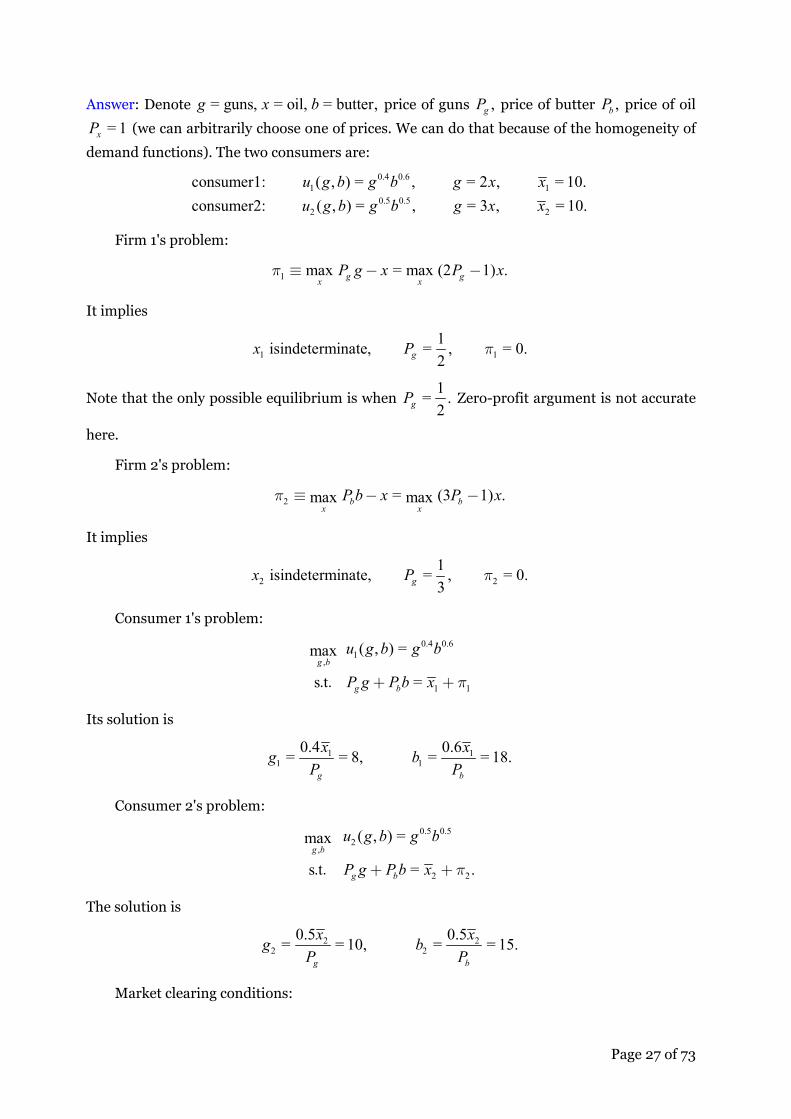
Answer: Denote = guns, = oil, = butter,g x b price of guns ,gP price of butter ,bP price of oil

= 1xP (we can arbitrarily choose one of prices. We can do that because of the homogeneity of

demand functions). The two consumers are:

0.4 0.6

1 10.5 0.5

2 2

consumer1: ( , ) = , = 2 , = 10.consumer2: ( , ) = , = 3 , = 10.

u g b g b g x xu g b g b g x x

Firm 1's problem:

1 max = max (2 1) .g gx xP g x P xπ ≡ − −

It implies

1 11isindeterminate, = , = 0.2gx P π

Note that the only possible equilibrium is when 1= .2gP Zero-profit argument is not accurate

here.

Firm 2's problem:

2 = (3 1) .max maxb bx x

P b x P xπ ≡ − −

It implies

2 21isindeterminate, = , = 0.3gx P π

Consumer 1's problem:

0.4 0.61

,

1 1

( , ) =max

s t =g b

g b

u g b g b

P g P b x π. . + +

Its solution is

1 11 1

0.4 0.6= = 8, = = 18.g b

x xg bP P

Consumer 2's problem:

0.5 0.52

,

2 2

( , ) =max

s t = .g b

g b

u g b g b

P g P b x π. . + +

The solution is

2 22 2

0.5 0.5= = 10, = = 15.g b

x xg bP P

Market clearing conditions:

Page 28 of 73

1 2 1 2 1 2 1 1 2 2= , = 2 , = 3 .x x x x g g x b b x+ + + +

Because of Walras Law, we only need two of these three conditions to determine the equilib-

rium. They imply that 1 = 9x∗ and 2 = 11.x∗ Therefore, the equilibrium is:

1 2 1 2 1 21 1= 9, = 11, = 8, = 10, = 18, = 15, = , = .2 3g bx x g g b b P P∗ ∗ ∗ ∗ ∗ ∗ ∗ ∗

Exercise 4.7. Suppose that there are one consumer, one firm, and one good .x The firm is

owned by the consumer. The consumer has an endowment of 1 unit of time for working and

enjoying leisure, and has utility function ( , ) = ln (1 ) lnu x y a x a y+ − for good x and leisure

time .y The firm inputs l amount of labor to produce =x al amount of good. Find the com-

petitive equilibrium.

Answer: Firm's problem:

,

= max = max ( ) .x l l

px wl ap w lπ − −

The solution is

, if > ,= 0, ], if = ,

0, if < .

d

ap wl ap w

ap w

⎧∞⎪⎪⎪⎪ ∞⎨⎪⎪⎪⎪⎩

The only possible equilibrium is when = 0.ap w− We thus only consider

isindeterminate, = , = 0.d s dl x al π

Consumer's problem:

1

,( , ) =max

s t = 1

a a

x yu x y x y

px wy w π

−

. . + ⋅ +

gives solution

(1 )= , = = 1 .d daw a wx y a

p w−

−

Market clearing conditions:

= 1, = .d d d sl y x x+

Because of Walras Law, we only need to use one of conditions to determine the equilibrium.

The first condition implies that = .l a∗ Then, 2= = ,x al a∗ ∗ and = awxp

∗ implies = .w ap

∗⎛ ⎞⎟⎜ ⎟⎜ ⎟⎜ ⎟⎝ ⎠

Therefore, the equilibrium is:

2= , = , = .wl a x a ap

∗

∗ ∗⎛ ⎞⎟⎜ ⎟⎜ ⎟⎜ ⎟⎝ ⎠

Page 29 of 73

Exercise 4.8. Suppose that the economy is the same as in Exercise 4.7 except that the firm

has production function = .x l Find the competitive equilibrium.

Answer: We can arbitrarily set = 1.p Firm's problem:

,

= = ,max maxx l l

x wl l wlπ − −

gives

21 1 1 1= = = , = .

4 2 42d sw l x

w w wlπ⇒ ⇒

Consumer's problem:

1

,( , ) =max

s t = 1

a a

x yu x y x y

x wy w π

−

. . + ⋅ +

gives solution

2

( ) 1 (1 )( ) 1= = , = = (1 ) 1 .1 4 4

d da w a wx a w y aw w w

π π⎛ ⎞ ⎛ ⎞+ − +⎟ ⎟⎜ ⎜+ − +⎟ ⎟⎜ ⎜⎟ ⎟⎜ ⎜⎝ ⎠ ⎝ ⎠

Market clearing conditions:

= 1, = .d d d sl y x x+

Because of Walras Law, we only need to use one of conditions to determine the equilibrium. It

implies that 2= .

4aw

a∗ −

Therefore, the equilibrium is:

2 1= , = , = , = .

2 2 4 2 2a a w a al x

a a p a aπ

∗

∗ ∗⎛ ⎞ −⎟⎜ ⎟⎜ ⎟⎜ ⎟− − −⎝ ⎠

Exercise 4.9. There are two goods x and y with prices xp and ,yp respectively, and two

individuals 11( , ) =u x y x yα α− and 1

2 ( , ) =u x y x yβ β− with 1 1 1= ( , )w x y and 2 2 2= ( , ).w x y

(a) Derive the contract curve. Suppose 0 < < < 1.α β Draw it in an Edgeworth box.

(b) Derive the equilibrium price ratio(s) / .x yp p p≡

Answer: (a) We have

1 2 1 2

1 2 1 2

1 2

1 2

( )= =(1 ) (1 )( )

(1 ) ( )=(1 )( ) ( )

x x

y y

u u y y yyu u x x x x

y y xyx x x

βαα β

α βα β β α

+ −⇒

− − + −

− +⇒

− + + −

which gives the contract curve as x goes from = 0x to 1 2= .x x x+ We have

Page 30 of 73

1 2 1 22

1 2

(1 ) (1 )( )( )= > 0,[ (1 )( ) ( ) ]x

x x y yyx x x

α α β βα β β α

− − + +− + + −

1 2 1 23

1 2

(1 ) (1 )( )( )= 2( ) < 0.[ (1 )( ) ( ) ]xx

x x y yyx x x

α α β ββ α

α β β α− − + +

− −− + + −

y

xy

ω

A

B

.x

Au

Bu

.

Contract curve

Figure 4.3. Contract Curve and Equilibrium

(b) We have

1 1 1 2 2 21 2

( ) ( )= = , = = .I px y I px yx xp p p pα α β β+ +

Equilibrium condition

1 2 1 2=x x x x+ +

implies

1 2 1 1 2 2( ) = ( ) ( )p x x px y px yα β+ + + +

which can be solved to get the equilibrium price ratio

1 2

1 2

= .(1 ) (1 )

y ypx x

α βα β

+− + −

Exercise 4.10. There are two goods x and ,y and two individuals

1 2( , ) = ( , ) = min{ , }u x y u x y x y

with 1 = (3,6)w and 2 = (7, 4).w

(a) Find all the Pareto optimal allocations. Are they strongly Pareto optimal?

(b) Find all the equilibrium price ratio(s) / .x yp p p≡

Answer: (a) The contract curve is the diagonal line in the chart. The points on the contract

curve are strongly P.O.

Page 31 of 73

.

x

y

1

2

contract line

W

1u.

2u

Figure 4.4. Contract Curve and Equilibria

(b) The set of equilibria is { | 0 }.p p≤ ≤ ∞ That is, all the possible values of /x yp P P≡

are equilibria.

5. Exercises for Chapter 5 There are no exercises for Chapter 5.

6. Exercises for Chapter 6 Exercise 6.1. You have just been asked to run a company that has two factories producing

the same good and sells its output in a perfectly competitive market. The production function

for each factory is:

= , = 1, 2.i i iy K L i

Initially, the capital stocks in the two factories are respectively 1 = 25K and 2 = 100.K The

wage rate for labor is ,w and the rental rate for capital is .r In the short run, the capital stock

for each factory is fixed, and only labor can be varied. In long run, both capital and labor can

be varied.

(a) Find the short-run total cost function for each factory.

(b) Find the company's short-run supply function of output and demand functions for labor.

(c) Find the long-run total cost function for each factory and the long-run supply curve of the

company.

(d) If all companies in the industry are identical to your company, what is the long-run indus-

try equilibrium price?

(e) Let = 1.r Suppose the cost of labor services increases from $1.00 to $2.00 per unit. What

is the new long-run industry equilibrium price? Can you determine whether the quantity

Page 32 of 73

of capital used in the long run will increase or decrease as a result of the increase in the

wage rate from $1.00 to $2.00 ?

Answer: (a) For each factory with capital stock ,K

{ } 2( , ) min | = = .L

wc y K wL rK y KL y rKK

≡ + +

Therefore, the short-run cost functions are

2 21 2( ) = 25 , ( ) = 100 .

25 100w wc y y r c y y r+ +

(b) The firm cares about the total profit from its two factories. The objective of firm is

therefore to maximize the total profit:

1 2

1 2 1 1 2 2,= max ( ) ( ) ( ).

y yp y y c y c yπ ⋅ + − −

The FOCs give us the well-known equality:

1 2= = .p MC MC

We have 12( ) =25wMC y y and 2 ( ) = .

50wMC y y Then 1 1= ( )p MC y and 2 2= ( )p MC y imply

that 12=25wp y and 2= .

50wp y Thus, 1

25=2

pyw

and 250= .py

w Therefore, the short-run

supply function is:

1 225 50= = = 62.5 .2

p py y y pw w w

⎛ ⎞⎟⎜+ + ⎟⎜ ⎟⎜⎝ ⎠

The labor demands for the factories are:

2 2 2 2

2 21 1 2 2

1 2

1 1 25 25 1 1 50= = = , = = = 25 .25 2 4 100

p p p pL y L yK w w K w w

⎛ ⎞ ⎛ ⎞ ⎛ ⎞ ⎛ ⎞⎟ ⎟ ⎟ ⎟⎜ ⎜ ⎜ ⎜⎟ ⎟ ⎟ ⎟⎜ ⎜ ⎜ ⎜⎟ ⎟ ⎟ ⎟⎜ ⎜ ⎜ ⎜⎝ ⎠ ⎝ ⎠ ⎝ ⎠ ⎝ ⎠

Therefore, the labor demand is

2

1 2125= = .

4pL L Lw

⎛ ⎞⎟⎜+ ⎟⎜ ⎟⎜⎝ ⎠

(c) The cost for each factory is

{ },

( ) min | = .i i iL Kc y wL rK y KL≡ +

The Lagrange function is

( ),iwL rK y KLλ≡ + + −L

implying

Page 33 of 73

= , = .i i i iw rL y K yr w

The total cost is then

1 1 2 2 1 2( ) = ( ) ( ) = 2 ( ) = 2 .c y c y c y wr y y y wr+ +

From the profit function = ( ) = ( 2 ) ,py c y p wr yπ − − we immediately find the long-run

supply function:

if > 2

= [0, ] if = 2

0 if < 2 .

s

p wr

y p wr

p wr

⎧⎪∞⎪⎪⎪⎪ ∞⎨⎪⎪⎪⎪⎪⎩

That is, the long-run industry supply curve is horizontal.

(d) In a competitive market, with a horizontal industry supply curve, the long-run equilib-

rium price must be = 2 ,p wr whatever the industry demand curve is.

(e) The original long-run equilibrium price is = 2,p and the new price is = 2 2.p The

total capital investment is

( )1 2 1 2= = = .r rK K K y y yw w

+ +

With an increase in w and ,p output y is reduced, implying K will be reduced.

p

p

y

sy

D

..

Exercise 6.2. Suppose that two identical firms are operating at the cooperative solution and

that each firm believes that if it adjusts its output the other firm will adjust its output to keep

its market share equal to 1 .2

What kind of industry structure does this imply?

Answer: Let ( )p Y be the market price of the good when the output is ,Y ( )ic y is the cost of

firm i when its output is .iy The two firms have the same cost function. The cartel maximizes

their total profit:

Page 34 of 73

1 2

1 2 1 2 1 2,

( )( ) ( ) ( ).max iy y

p y y y y c y c yπ ≡ + + − −

The FOCs are

( ) ( ) = ( ).ip Y p Y Y c y∗ ∗ ∗ ∗′ ′+ (12)

We look for a solution for which 1 2=y y∗ ∗ (the symmetric solution). Thus, the FOC becomes

( ) ( ) = .2

Yp Y p Y Y c∗

∗ ∗ ∗⎛ ⎞⎟⎜′ ′ ⎟+ ⎜ ⎟⎜ ⎟⎝ ⎠

(13)

We can rewrite (13) as

( ) = ,2

YMR Y c∗

∗⎛ ⎞⎟⎜′ ⎟⎜ ⎟⎜ ⎟⎝ ⎠

where ( ) ( ) .R Y p Y Y≡ On the other hand, the Cournot output is determined by

1( ) ( ) = .2 2

YMR Y p Y Y c∗

∗ ∗ ∗⎛ ⎞⎟⎜′ ′ ⎟− ⎜ ⎟⎜ ⎟⎝ ⎠

.

p

Y

B A

)(YMR

2Yc

⎛ ⎞⎟⎜′ ⎟⎜ ⎟⎜⎝ ⎠

D1( ) ( )2

MR Y p Y Y′−

.C .

Figure 6.1. A market-share Cournot equilibrium

In the diagram, point A is the ‘competitive solution,’ for which each firm takes the market

price as given; point B is our solution, for which each firm acts upon a decreasing demand

and assume equal market share as the other's reaction; point C is the Cournot equilibrium.

From the diagram, we can conclude that

• The equilibrium output at B is lower than the output at the ‘competitive solution’ and the

output at the Cournot equilibrium.

• The equilibrium price at B is higher than the price at the ‘competitive solution’ and the

price at the Cournot equilibrium.

Exercise 6.3. Consider an industry with two firms, each having marginal costs equal to zero.

The industry demand is

Page 35 of 73

( ) = 100 ,P Y Y−

where 1 2=Y y y+ is total output.

(a) What is the competitive equilibrium output?

(b) If each firm behaves as a Cournot competitor, what is firm 1's optimal output given firm 2's

output?

(c) Calculate the Cournot equilibrium output for each firm.

(d) Calculate the cooperative output for the industry.

(e) If firm 1 behaves as a follower and firm 2 behaves as a leader, calculate the Stackelberg

equilibrium output of each firm.

Answer: (a) For competitive output, firms take price as given in maximizing their own profits:

max ,i iPyπ ≡

which implies

if > 0

=[0, ) if = 0.i

Py

P∗

⎧+∞⎪⎪⎨⎪ + ∞⎪⎩

That is, the firms' supply curve is the horizontal line at = 0.P So is the industry supply curve.

The equilibrium industry supply is thus = 100Y ∗ and the equilibrium price is = 0.P∗

(b) Firm 1 maximizes his own profit, given any 2 :y

1 2 1 1 2 1max ( ) = (100 ) ,i P y y y y y yπ ≡ + − −

which gives the FOC:

1 2100 2 = 0.y y− −

Firm 1's reaction function is thus 1 21ˆ = (100 ).2

y y−

(c) By symmetry, the outputs for the two firms should be the same in equilibrium. By the

reaction function in (b), we hence have 1 11= (100 ),2

y y− which gives 1100= .

3y Therefore,

the Cournot equilibrium is

1 2100= = .

3y y∗ ∗

(d) Suppose the two firms collude. They form a monopoly and maximizes their total profit:

max ( ) = (100 ) ,P Y Y Y Yπ ≡ −

which gives the cartel output: = 50.Y ∗

Page 36 of 73

(e) Firm 1 will behave as in (b), and reacts according to his reaction function

1 21ˆ = (100 ).2

y y− Firm 2 will take this into consideration when maximizing his own profit:

2 1 2 2 2 2 21ˆmax [ ( ) ] = (100 ) ,2

P y y y y y yπ ≡ + −

which implies 2 = 50.y∗ Then, 1 = 25.y∗

In summary, the competitive industry output is the highest, the Stackelberg industry out-

put is the second, the Cournot industry output is the third, and cartel output is the lowest.

Exercise 6.4. Consider a Cournot industry in which the firms’ outputs are denoted by

1, , ,ny y… aggregate output is denoted by =1

= ,nii

Y y∑ the industry demand curve is denoted

by ( ),P Y and the cost function of each firm is given by ( ) = .i i ic y cy For simplicity, assume

( ) < 0.P Y′′ Suppose that each firm is required to pay a specific tax of it on output.

(a) Devise the first-order conditions for firm .i

(b) Show that the industry output and price only depend on the sum of tax rates =1

.nii

t∑

(c) Consider a change in each firm's tax rate that does not change the tax burden on the indus-

try. Letting itΔ denote the change in firm i 's tax rate, we require that =1

= 0.nii

tΔ∑ As-

suming that no firm leaves the industry, calculate the change in firm i 's equilibrium out-put .iyΔ [Hint: use the equations from the derivations of (a) and (b)].

Answer: (a) The profit maximization for firm i is

=1

max = ( ) .n

i j i i ij

P y y k t yπ⎛ ⎞⎟⎜ ⎟ − +⎜ ⎟⎜ ⎟⎜⎝ ⎠∑

The FOC is

( ) ( ) = .i iP Y P Y y k t′+ + (14)

(b) By summarizing (14) from = 1i to ,n we have

=1

( ) ( ) = .n

ij

nP Y P Y Y nk t′+ + ∑ (15)

This equation determines the industry output ,Y which obviously depends on =1

,n

ij

t∑ rather

than the individual tax rates it 's.

(c) Since the total output depends only on =1

n

ij

t∑ and the latter has no change, Y doesn't

change for a tax change. Then, by (14), = ( ) ,i it P Y y′Δ Δ i.e.,

Page 37 of 73

= ,( )

ii '

tyP YΔ

Δ

where Y is determined by (15).

Exercise 6.5 (Entry Cost in a Bertrand Model). Consider an industry with an entry cost. Let

( ) = , ( ) = ,dic y cy p y a y−

where > 0a and 0c ≥ are two constants. Find the equilibrium solution for the following two-

stage game.

Stage 1. All potential firms simultaneously decide to be in or out. If a firm decides to be in, it

pays a setup cost > 0.K

Stage 2. All firms that have entered play a Bertrand game.

Answer: This is from Example 12.E.2 on page 407 of MWG (1995). Once n identical firms are

in the industry, they play a Bertrand game. As we know, if 0,n ≥ the result is the competitive

outcome, i.e., =p c∗ and the profit without including the entry cost K is zero for all the firms.

This means that each firm loses K in the long run. Knowing this, once one firm has entered

the industry, all other firms will stay out. Therefore, more intense competition in stage 2

results in a less competitive industry!

This single firm will be the monopoly and produces at the monopolist output = ,2m

a cqb

−

resulting the monopoly price = .2m

a cp + The monopoly profit is

2( )= .

4ma c K

b−

Π −

As long as 0,mΠ ≥ a firm will enter and that is the only firm in the industry.

Exercise 6.6. Verify the socially optimal number of firms to be 2/3

1/3

( )= 1o a cnK−

− in Section

6.9.

Answer: We have

2 2

0

22

2

1( ) = ( ) = ( )2

1=2 1 1

1= ( )1 2 1 1

nny

n n nW n a y dy ncy nK a a ny cny nK

a c a ca a n cn nKn n

n a c a ca a c n cn nKn n n

⎡ ⎤− − − − − − −⎢ ⎥⎣ ⎦

⎡ ⎤⎛ ⎞− −⎢ ⎥⎟⎜− − − −⎟⎜⎢ ⎥⎟⎜⎝ ⎠+ +⎢ ⎥⎣ ⎦⎛ ⎞− −⎟⎜− − − −⎟⎜ ⎟⎜⎝ ⎠+ + +

∫

Page 38 of 73

22

22

2 2

1= ( )1 2 1

1= 2 ( )2 1 1

1= 1 (1 ) ( ) ,2 1

n a ca c n nKn n

n n a c nKn n

a c Kγγ

γ

⎛ ⎞− ⎟⎜− − −⎟⎜ ⎟⎜⎝ ⎠+ +⎡ ⎤⎛ ⎞⎢ ⎥⎟⎜− − −⎟⎜⎢ ⎥⎟⎜⎝ ⎠+ +⎢ ⎥⎣ ⎦

⎡ ⎤− − − −⎢ ⎥⎣ ⎦ −

where .1

nn

γ ≡+

Then,

220 = = (1 )( ) ,

(1 )W Ka cγγ γ

∂− − −

∂ −

implying

1/3

2= 1 ,( )

o Ka c

γ⎡ ⎤⎢ ⎥− ⎢ ⎥−⎣ ⎦

implying

1/3

2 2/3

1/3 1/3

2

1( ) ( )= = = 1.

1

( )

oo

o

Ka c a cn

KKa c

γγ

⎡ ⎤⎢ ⎥−⎢ ⎥− −⎣ ⎦ −

− ⎡ ⎤⎢ ⎥⎢ ⎥−⎣ ⎦

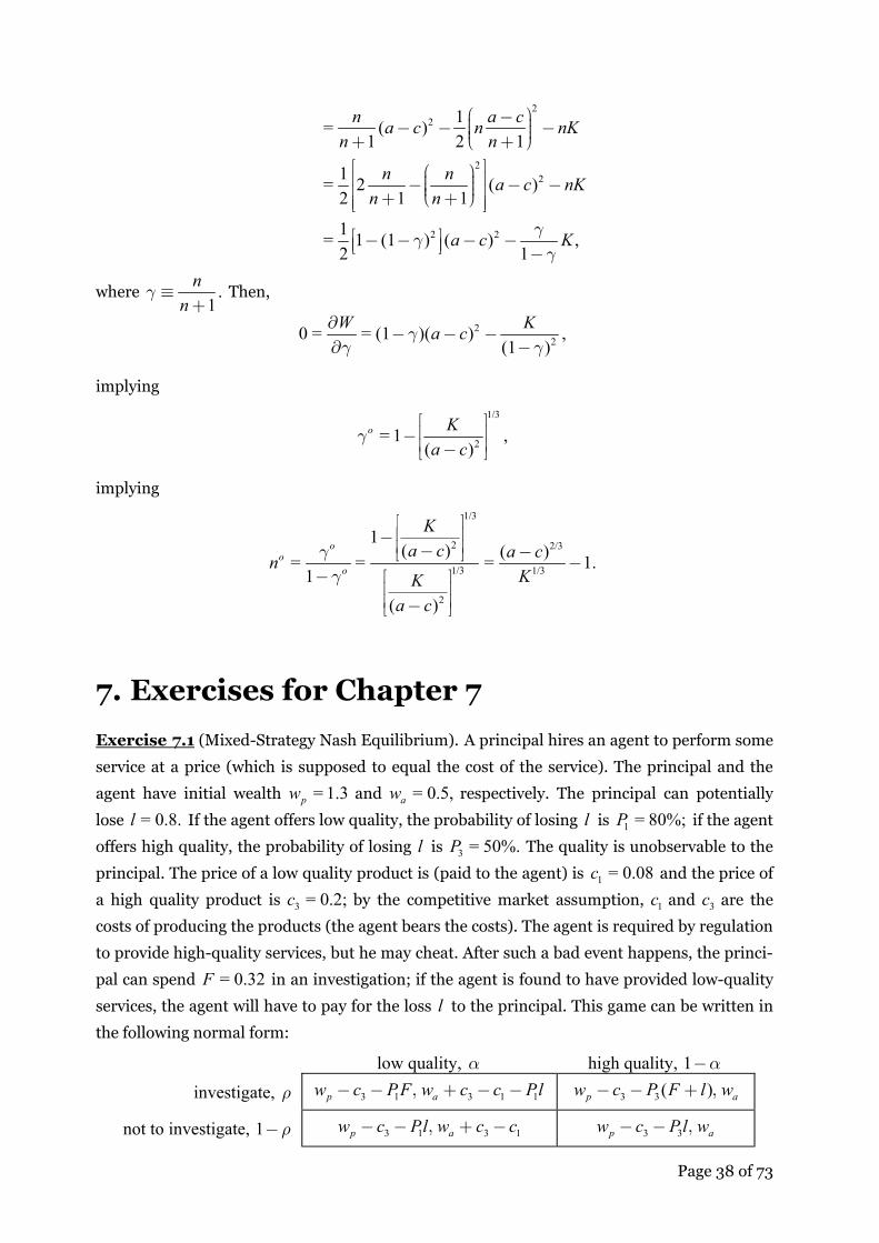
7. Exercises for Chapter 7 Exercise 7.1 (Mixed-Strategy Nash Equilibrium). A principal hires an agent to perform some

service at a price (which is supposed to equal the cost of the service). The principal and the

agent have initial wealth = 1.3pw and = 0.5,aw respectively. The principal can potentially

lose = 0.8.l If the agent offers low quality, the probability of losing l is 1 = 80%;P if the agent

offers high quality, the probability of losing l is 3 = 50%.P The quality is unobservable to the

principal. The price of a low quality product is (paid to the agent) is 1 = 0.08c and the price of

a high quality product is 3 = 0.2;c by the competitive market assumption, 1c and 3c are the

costs of producing the products (the agent bears the costs). The agent is required by regulation

to provide high-quality services, but he may cheat. After such a bad event happens, the princi-

pal can spend = 0.32F in an investigation; if the agent is found to have provided low-quality

services, the agent will have to pay for the loss l to the principal. This game can be written in

the following normal form:

low quality, α high quality, 1 α− investigate, ρ 3 1 3 1 1p aw c P F w c c Pl− − , + − − 3 3( )p aw c P F l w− − + ,

not to investigate, 1 ρ− 3 1 3 1p aw c Pl w c c− − , + − 3 3p aw c P l w− − ,

Page 39 of 73

where

= probabilityoftheprincipalinvestigating,= probabilityofagentdeliveringlowquality.

ρα

Find the mixed-strategy Nash equilibria.

Answer: Assume that the principal can commit ex ante to investigate or not before a loss oc-

curs. In other words, the principal can only make up his mind on investigation before she has

suffered a loss. Before a loss occurs, the game box of surpluses is

low quality, α high quality, 1 α−

investigate, ρ 3 1 3 1 1p aw c P F w c c Pl− − , + − − 3 3( )p aw c P F l w− − + ,

not to investigate, 1 ρ− 3 1 3 1p aw c Pl w c c− − , + − 3 3p aw c P l w− − ,

In each cell, the value on the left is the surplus of the principal and the value on the right is the

surplus of the agent.

The optimal choice of α is to make the principal indifferent between investigation and no

investigation:

( ) ( ) ( )3 1 3 3 1 31 = 1 ,p pw c P F P F l w c Pl P lα α α α− − − − + − − − − (16)

implying

( )1 3 11 = ,P F P F Plα α α− − − −

implying

( )1 3 1 3= ,Pl P F P F P Fα + −

implying

3

1 3 1

0.5 0.32= = = 0.29.0.8 0.8 0.5 0.32 0.8 0.32

P FPl P F P F

α×

+ − × + × − ×

The choice of ρ is to make the agent indifferent between cheating and no cheating:

3 1 1 = ,a aw c c Pl wρ+ − − (17)

implying

3 1

1

0.20 0.08= = = 0.19.0.8 0.8

c cPl

ρ− −

×

Exercise 7.2 (Pure-Strategy Nash Equilibrium). Find the pure-strategy Nash equilibria in the

above exercise.

Answer: By substituting the parameter values into the game box of surpluses, we have

cheat, α not to cheat, 1 α− investigate, ρ 0 84 0 02. , − . 0 54 0 5. , .

Page 40 of 73

not to investigate, 1 ρ− 0 46 0 62. , . 0 7 0 5. , . By Proposition 7.2, to find pure-strategy Nash equilibria, we can restrict to pure strategies

only. Thus, simply by inspecting each cell one by one, we know that there is no pure-strategy

Nash equilibrium.

Exercise 7.3. For the following game, find the pure-strategy NEs. Show whether or not they

are trembling-hand perfect.

Player 2 2L 2R

Player 1 : 1L 1, 6 0, 5 1R 1, 1 1, 2

Answer: This is a situation in which a player is indifferent from two alternative strategies, one

of which is the equilibrium strategy. This player has no incentive to deviate if other players

don't make any mistakes. However, the situation changes if possible mistakes by other players

are taken into account. There two NEs: 1 2( , )L L and 1 2( , ).R R In 1 2( , ),L L given 2 ,L player 1 is

indifferent from 1L and 1.R However, if player 2 may make some mistakes by taking 1R with

probability > 0,ε no matter how small ε is, player 1 will be strictly prefer 1R to 1.L Thus,

1 2( , )L L is not a trembling-hand NE, while 1 2( , )R R is.

Exercise 7.4. For the game in Example 7.14, find all the pure-strategy Nash equilibria.

Answer: The strategy sets for players 1 and 2 are simple:

1 1 1 2 2 2= { , }, = { , }.L R L RS S

There are three information sets for player 3. Denote a typical strategy of player 3 as

3 1 2 3= ( , , ),s a a a where 1a is the action if the information set on the left is reached, 2a is the

action if the information set in the middle is reached, and 3a is the action if the information

set on the right is reached. Player 3 has eight strategies:

13 23 33 43

53 63 73 83

= ( , , ), = ( , , ), = ( , , ), = ( , , ),= ( , , ), = ( , , ), = ( , , ), = ( , , ).

s l l l s r l l s l l r s r l rs l r l s r r l s l r r s r r r

The normal form is

P1 plays 1L P3 13s 23s 33s 43s 53s 63s 73s 83s

P2: 1L 2,0,1 -1,5,6 2,0,1 -1,5,6 2,0,1 -1,5,6 2,0,1 -1,5,6 2R 2,0,1 -1,5,6 2,0,1 (-1,5,6) 2,0,1 -1,5,6 2,0,1 (-1,5,6)

P1 plays 1R P3 13s 23s 33s 43s 53s 63s 73s 83s

P2: 2L 3,1,2 3,1,2 3,1,2 3,1,2 (5,4,4) (5,4,4) (5,4,4) (5,4,4) 2R 0,-1,7 0,-1,7 -2,2,0 -2,2,0 0,-1,7 0,-1,7 -2,2,0 -2,2,0

Page 41 of 73

All the pure strategy Nash equilibria are indicated in the boxes.

To find all the Nash equilibria, we can check each cell one by one. A cell cannot be a Nash

equilibrium if one of the players doesn't stick to it. In each cell, we can first check to see if

player 3 will stick to his strategy, by which we can quickly eliminate many cells.

A sequentially rational NE must be an outcome from backward induction. Example 7.14

shows that backward induction only leads to one outcome: 1 1 2 2 3 53= , = , = ,s R s L s s which is

one of the Nash equilibria.

Exercise 7.5. In Example 7.16, explain why there are mixed-strategy NEs in which P1 mixes

1M and 1R arbitrarily and P2 chooses 2.R

Answer: ?

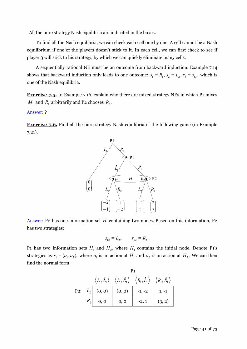
Exercise 7.6. Find all the pure-strategy Nash equilibria of the following game (in Example

7.21).

o

21

⎛ ⎞− ⎟⎜ ⎟⎜ ⎟⎟⎜−⎝ ⎠

P1

. .

12

⎛ ⎞⎟⎜ ⎟⎜ ⎟⎟⎜−⎝ ⎠1

1⎛ ⎞− ⎟⎜ ⎟⎜ ⎟⎟⎜⎝ ⎠

23

⎛ ⎞⎟⎜ ⎟⎜ ⎟⎟⎜⎝ ⎠

P200

⎛ ⎞⎟⎜ ⎟⎜ ⎟⎟⎜⎝ ⎠

H

1L

1̂L

2L 2R 2R2L

1μ 2μ

.1R̂

1R

P1

x

Answer: P2 has one information set H containing two nodes. Based on this information, P2

has two strategies:

12 2 22 2= , = .s L s R

P1 has two information sets 1H and 2 ,H where 1H contains the initial node. Denote P1's

strategies as 1 1 2= , ,s a a⟨ ⟩ where 1a is an action at 1H and 2a is an action at 2 .H We can then

find the normal form:

P1

1 1̂,L L 1 1ˆ,L R 1 1̂,R L 1 1

ˆ,R R

P2: 2L (0, 0) (0, 0) -1, -2 1, -1

2R 0, 0 0, 0 -2, 1 (3, 2)

Page 42 of 73

We can easily find the pure-strategy Nash equilibria, as indicated in the above box. Among

these three NEs, there is one SPNE, which is

1 1 1 2 2ˆ= , , = .s R R s R

Given ( )1 2= , ,μ μ μ P2 chooses 2L iff 1 2 1 2> 2 3μ μ μ μ− + − + or 1 > 2/3.μ If so, P1

chooses 1R̂ at node .x Then, since choosing 1R means a payoff of 1,− P1 chooses 1L at the

beginning. Hence, any belief system with 1 > 2/3μ can support a BE that leads to the payoff

pair (0, 0). Such a BE is:

1 1 1 2 2 12ˆ= , , = , .3

s L R s L μ∗ ∗ ∗⟨ ⟩ > (18)

By a similar argument and with the consistency of beliefs on the equilibrim path, there is

another BE in which P2 chooses 2R :

1 1 1 2 2 2ˆ= , , = , 1.s R R s R μ∗ ∗ ∗⟨ ⟩ = (19)

Further, if 1 2 / 3,μ = P2 is indifferent between 2L and 2.R Let P2’s mixed strategy in this case

be 2 ( ,1 ),t tσ = − where [0, 1].t ∈ If H is on the equilibrium path, since 1 (0, 1),μ ∈ P1 must

be indifferent between 1̂L and 1ˆ .R This turns out to be impossible. Hence, there is no BE in

this case. Hence, there are only two possible BEs, which are in (18) and (19).

Since the BE in (18) is not a SPNE, we conclude that BEs may not be SPNEs.

Exercise 7.7. A revised version of Exercise 9.C.7 in Mas-Colell et al. (1995, p.304)].

(a) For the following game in Figure 7.1, find all the pure-strategy NEs. Which one is the

SPNE?

o

P2

⎟⎠

⎞⎜⎝

⎛24

..

P1

⎟⎠

⎞⎜⎝

⎛22

1δ 2δ

1γ 2γ

1δ 2δ

B T

D U D U

⎟⎠

⎞⎜⎝

⎛11

⎟⎠

⎞⎜⎝

⎛15

P2

Figure 7.1. NEs and SPNEs

(b) Now suppose that P2 cannot observe P1's move. Draw the game tree, and find all the

mixed-strategy NEs.

(c) Following the game in (b), now suppose that P1 may make a mistake in implementing his

strategies. Specifically, after P1 has decided to play ,T he may actually implement T with

probability p and mistakenly implement B with probability 1 ;p− symmetrically, after

Page 43 of 73

P1 has decided to play ,B he may actually implement B with probability p and mistak-

enly implement T with probability 1 .p− 2 Draw the game tree and find all the BEs.

Answer: (a) There are two information sets for P2. Let 1 2( , )a a be a typical P2's strategy,

where 1a is an action taken at the left information set and 2a is an action taken at the right

information set. The normal form of the game is

P2

(D, D) (D, U) (U, D) (U, U)

P1: B 4, 2 (4, 2) 1, 1 1, 1

T 5, 1 2, 2 5, 1 (2, 2)

There are two pure-strategy NEs: = [ , ( , )]B D Uσ∗ and = [ , ( , )].T U Uσ∗ The first one is the

SPNE.

(b) The game tree is:

o

P2

⎟⎠

⎞⎜⎝

⎛24

..

P1

⎟⎠

⎞⎜⎝

⎛22

1δ 2δ2H

1γ 2γ

1δ 2δ

B T

D U D U

⎟⎠

⎞⎜⎝

⎛11

⎟⎠

⎞⎜⎝

⎛15

The normal form is

P2 D U

P1: B 4, 2 1, 1 T 5, 1 (2, 2)

There is a pure-strategy NE: = ( , ).T Uσ∗ Since playing T is a strictly dominant strategy for

P1, this NE is the only mixed-strategy NE.

(c) The game tree is

2 In Mas-Colell et al. (1995), it is P2 who may make a mistake in observing P1's strategies. In this case, there

is no mistake in implementation; it is just a mistake in identifying the actual strategy.

Page 44 of 73

o

P2

⎟⎠

⎞⎜⎝

⎛24

..

P1

21 )1( γγ pp −+

⎟⎠

⎞⎜⎝

⎛22

1δ 2δ2H

1γ 2γ

12 )1( γγ pp −+

1δ 2δ

B T

D U D U

⎟⎠

⎞⎜⎝

⎛11

⎟⎠

⎞⎜⎝

⎛15

Figure 7.2.

In this game tree, the beliefs are

1 1 2 2 2 1= (1 ) , = (1 ) ,p p p pμ γ γ μ γ γ+ − + −

which are derived from Bayes rule by allowing the possibility of an error in implementation,

where 0iγ ≥ and 1 2 = 1.γ γ+ We have 1 2 = 1.μ μ+ We can also have the following game

tree, where P2's beliefs are also derived from Bayes rule. Since the two game trees are equiva-

lent, we will thus use Figure 7.2 only.

o

P2 ..

P1

1γp2H

1γ 2γ

2γp

B T

⎟⎠

⎞⎜⎝

⎛24

D U

⎟⎠

⎞⎜⎝

⎛11

Nature

p p−1 p−1pB BT T

1)1( γp−

⎟⎠

⎞⎜⎝

⎛15

D U

⎟⎠

⎞⎜⎝

⎛22 ⎟

⎠

⎞⎜⎝

⎛15

D U

⎟⎠

⎞⎜⎝

⎛22⎟

⎠

⎞⎜⎝

⎛24

D U

⎟⎠

⎞⎜⎝

⎛11

.

. .

.

2)1( γp−

We now solve for BEs in the game tree of Figure 7.2. We solve by backward induction. We

find

1 2 1 2 2 12 > 2 (1 2 ) > (1 2 ) .D U p pμ μ μ μ γ γ⇔ + + ⇔ − − (20)

Then, first, if ,D U P1 will choose ,T i.e., 1 = 0γ and 2 = 1.γ To be consistent with (20), we

need 1< .2

p Thus, we have one BE when 1< :2

p 1 = 0γ∗ and 1 = 1.δ∗

Second, if ,D U≺ P1 will also choose ,T i.e., 1 = 0γ and 2 = 1.γ To be consistent with

(20), we need 1> .2

p Thus, we have another BE when 1> :2

p 1 = 0γ∗ and 1 = 0.δ∗

Page 45 of 73

Third, if ,D U∼ (20) implies 2 1(1 2 ) = (1 2 ) .p pγ γ− − If 1 ,2

p ≠ we have 1 2= ,γ γ i.e.,

1= .2iγ P1 compares the expected profits for the two choices: 1 2= 4Bπ δ δ+ and

1 2= 5 2 .Tπ δ δ+ Since > ,T Bπ π P1 chooses ,T i.e., 1 = 0γ and 2 = 1,γ which is inconsistent

with 1= .2iγ If

1= ,2

p we still have 1 2= 4Bπ δ δ+ and 1 2= 5 2 .Tπ δ δ+ Since > ,T Bπ π P1

chooses ,T i.e., 1 = 0γ and 2 = 1.γ Thus, we have another BE when 1= :2

p 1 = 0γ∗ and 1δ∗

can be any value in [0, 1].

In summary, we have three BEs:

Error BE

12p < P1 plays T, P2 plays D

12p > P1 plays T, P2 plays U

12p = P1 plays T, P2 plays any strategy (pure or mixed)

Exercise 7.8. One problem with a BE is that it may not be trembling-hand perfect. Consider

Example 7.10 with the game in Figure 7.3.

o

..

12

⎛ ⎞⎟⎜ ⎟⎜ ⎟⎟⎜⎝ ⎠33

⎛ ⎞⎟⎜ ⎟⎜ ⎟⎟⎜⎝ ⎠

02

⎛ ⎞⎟⎜ ⎟⎜ ⎟⎟⎜⎝ ⎠

01

⎛ ⎞⎟⎜ ⎟⎜ ⎟⎟⎜⎝ ⎠

P1

P22μ1μ

1L 1R

2L 2R 2L 2R

Figure 7.3. Trembling-Hand Perfect Equilibrium

(a) Show that we have the following BE:

1 1 2 2 1 2= , = , = 1, = 0,s L s L μ μ∗ ∗ ∗ ∗ ∗

with payoff pair (1, 2).

(b) Show that this BE is a SE. Note that we already know in Example 7.10 that this strategy

profile 1 2( , )s s∗ ∗ is not trembling-hand perfect. ■

Answer: It is simple. You do by yourself.

Page 46 of 73

8. Exercises for Chapter 8 Exercise 8.1 (Akerlof). In the Akerlof model, we now suppose that the buyers can be guar-

anteed a minimum quality of the car by inspection and test drive. Specifically, instead of the

minimum quality = 0q for used cars in the market, suppose that all the cars have a minimum

quality > 0.t

(1) Will adverse selection disappear?

(2) Is it possible to have cars with a range of qualities to be traded in the market?

Answer: Since the seller will still sell her car for a price ,p q≥ the car quality is uniformly

distributed along interval [ , ].t p Thus, the average quality of cars on the market is = .2

t pμ

+

Since there is demand if 3 ,2

pμ ≥ any car can be sold for 3 .p t≤ This means that any car with

quality 3t or less will be traded in the market, i.e., the seller with car quality 3q t≤ will be

able to find a buyer and trade the car at a price [ , 3 ].p q t∈ So, there is a market, and the

market is for cars with quality in the range 3 .t q t≤ ≤ However, it is still a market for lemons

since it is only for low-quality cars.

In summary, there is a range of qualities in which cars with those qualities are sold. How-

ever, adverse selection still exists, since only low-quality cars are chosen by sellers to be on the

market.

Exercise 8.2 (Akerlof). In the Akerlof model, what would be the result if we changed the

buyer's utility to

= 3 ?bU M qn+

That is, the buyer's MU for a car is now 3 ,q instead of 3 .2

q How will such an increase in desire

for a car change the results? Explain your conclusion intuitively.

Answer: For the case with asymmetric information, the decision rule for the buyer is 3p μ≤

and for the seller is still .p q≥ By the decision rule, the average quality is still = .2p

μ Thus,

any car can be sold and the buyer's decision is to buy any car at the market price. The intuition

is this: the buyer is desperate for a car so that as long as the price and quality are not too far apart, he will buy the car. Since all the used cars will be on the market, the mean is = 1.μ

Thus, the market price is = 2.p With this price, the buyer will buy any car and the seller is

willing to sell her car.

Page 47 of 73

Exercise 8.3 (RS Insurance). Consider the RS insurance model under complete informa-

tion. The insurance company offers a price q for an insurance policy that pays a compensation

qz if an accident happens. Let ( ) = ln( ).u I I

(a) Compute the demand functions 1 ( )dI q and 2 ( ).dI q

(b) Compute the slopes of demand 1 ( )dI qq

∂∂

and 2 ( )dI qq

∂∂

and interpret.

(c) Under what price would a person demands full insurance, i.e., 1 2( ) = ( )d dI q I q ?

Answer: (a) With ( ) = ln ,u I I the FOC becomes

2

1

(1 ) 1= .I qI qπ

π− −

(21)

The budget constraint is

1 2(1 ) = .q I qI w qL− + − (22)

The two equations (21) and (22) determine the two unknowns 1I and 2 .I The solution is

( ) ( )1 21= , = .1

d dI w qL I w qLq qπ π−

− −−

(23)

(b) The slopes of demand are

( )

( )1 22 2

( ) ( )1= > 0, = < 0.1

d dI q I qw L wq q qq

π π∂ ∂−− −

∂ ∂−

1dI and 2

dI are respectively the demands for income in good and bad times. The signs of the

slopes can be interpreted as: if the price of insurance against the bad time is high, the individ-

ual will buy less insurance for the bad time but will try to enjoy more in the good time.

(c) By (23), we find that 1 2( ) = ( )d dI q I q if and only if = .q π That is, only if the company

behaves like a perfectly competitive firm, the individual will choose full insurance.

Exercise 8.4 (RS Insurance). Consider the RS insurance model under asymmetric infor-

mation. Suppose that insurance companies offer price-quantity contracts. There are two types

of agents with type =i H or .L The initial wealth for all agents is .w An agent with type i has

the probability iπ of losing an amount L when the bad event happens. All agents have the

same initial wealth ,w the same possible loss L and the same utility function ( )u I of income

.I Let

1 3= 24, = 16, ( ) = 2 , = , = .2 4L Hw L u I I π π

(a) Compute the marginal rates of substitution for the two types and explain their relative

magnitudes.

Page 48 of 73

(b) Compute the separating equilibrium, assuming its existence.

(c) Determine the condition under which the separating equilibrium survives.

Answer: (a) The MRS is a typical person with probability π is

1

2

(1 ) ( )= .( )u IMRS

u Iπ

π′−

′

Thus, the MRS for the two types are respectively

2 2

1 1

1 1= , = .L HL H

L H

I IMRS MRSI I

π ππ π− −

At each point 1 2( , ),I I we always have > .L HMRS MRS That is, since the slope of an indiffer-

ence curve is the MRS, the indifference curve for type L is always steeper than the indifference

curve for type H at any point. The intuition is clear; since MRS is an individual's internal price

of the good time, type L values the good time highly since they are less likely to have a bad

time.

(b) The zero-profit line for type H is

1 2(1 ) = ,H H HI I w Lπ π π− + −

i.e.,

1 23 = 48.I I+

Thus, the point B on Figure 8.1 where 1 2=I I is (12,12).B ≡ The indifference curve going

through B is

1 2(1 ) ( ) ( ) = (12),H Hu I u I uπ π− +

i.e.,

1 23 = 4 12.I I+ (24)

. o

1I

2I

..Hu

Lu

A

pooling

Hπ

LπPπ

line°45

.D

*HC

*LC

.

Figure 8.1. Separating Equilibrium

Page 49 of 73

The zero-profit line for type L is

1 2(1 ) = ,L L LI I w Lπ π π− + −

i.e.,

1 2 = 32.I I+ (25)

Then, the point E on Figure 8.1 is determined jointly by (24) and (25):

1 2

1 2

= 32,

3 = 4 12.

I I

I I

+

+

To solve this equation set, let 1 1x I≡ and 2 2 .x I≡ Then,

2 21 2

1 2

= 32,

3 = 4 12.

x x

x x

+

+

It implies

22 25 24 3 80 = 0,x x− +

which gives

224 3 8 2 12 3 4 2= = .

10 5x ± ±

There are two possible values for 2.x As indicated by Figure 8.1, we should pick the lower

value. Thus,

2

1 2

12 3 4 2= ,5

4 3 12 2= 8 3 3 = .5

x

x x

−

+−

Hence, the point E is

= (22.85,9.15).E

The separating equilibrium is a set of contracts B and .E

(c) The indifference curve going through E is

( ) ( )1 2(1 ) ( ) ( ) = (1 ) 22.85 9.15 ,L L L Lu I u I u uπ π π π− + − +

i.e.,

1 2 = 7.8.I I+ (26)

The budget line for a pooling equilibrium is

1 2(1 ) = 24 16 ,P P PI Iπ π π− + −

Page 50 of 73

where 3 1= (1 ) = ,4 4P L Hπ λπ λ π λ+ − − and λ is the population proportion of type L. Thus,

( ) 1 21 3 11 = 12 4 .4 4 4

I Iλ λ λ⎛ ⎞⎟⎜+ + − +⎟⎜ ⎟⎜⎝ ⎠

(27)

In order for the separating equivalent to be sustainable, we need to show that (26) and (27)

don't intersect. In other words, we need to show that the following equation set has no solu-

tion:

( ) ( )

1 2

1 2

= 7.8,

1 3 = 48 16 .

I I

I Iλ λ λ

+

+ + − +

Again, let 1 1x I≡ and 2 2 .x I≡ The equation set now becomes

( ) ( )

1 22 21 2

= 7.8,

1 3 = 48 16 ,

x x

x xλ λ λ

+

+ + − +

which implies

( ) ( )( )221 11 3 7.8 = 48 16 ,x xλ λ λ+ + − − +

implying

( ) ( )21 14 15.6 3 60.84 3 = 48 16 ,x xλ λ λ− − + − +

implying

( )21 13.9 3 33.63 19.21 = 0.x xλ λ− − + −

As we know, an equation 2 = 0ax bx c+ + doesn't to have a solution if and only if 2 4 < 0.b ac− For our problem, this condition is

( ) ( )2

3.9 3 < 4 33.63 19.21 ,λ λ⎡ ⎤− −⎣ ⎦

i.e.,

29 6 < 8.84 5.05 ,λ λ λ− + −

i.e.,

2 0.95 0.16 < 0.λ λ− + (28)

The solutions of 2 0.95 0.16 = 0λ λ− + are

2 21 2

1 1= 0.95 0.95 0.64 = 0.73, = 0.95 0.95 0.64 = 0.22.2 2

λ λ⎡ ⎤ ⎡ ⎤+ − − −⎢ ⎥ ⎢ ⎥⎣ ⎦ ⎣ ⎦

As indicated by the following chart, (28) holds if and only if 0.22 < < 0.73.λ Therefore, when

the population share of type L is less than 73%, there exists a separating equilibrium, defined

by ( , ).B E

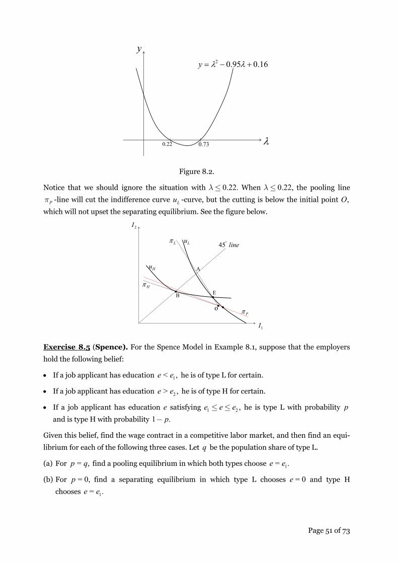
Page 51 of 73

22.0 73.0 λ

16.095.02 +−= λλy

y

Figure 8.2.

Notice that we should ignore the situation with 0.22.λ ≤ When 0.22,λ ≤ the pooling line

Pπ -line will cut the indifference curve Lu -curve, but the cutting is below the initial point ,O

which will not upset the separating equilibrium. See the figure below.

.o1I

2I

..

Hu

Lu

A

B

Hπ

Lπ

Pπ

line°45

E

.

Exercise 8.5 (Spence). For the Spence Model in Example 8.1, suppose that the employers

hold the following belief:

• If a job applicant has education 1< ,e e he is of type L for certain.

• If a job applicant has education 2> ,e e he is of type H for certain.

• If a job applicant has education e satisfying 1 2 ,e e e≤ ≤ he is type L with probability p

and is type H with probability 1 .p−

Given this belief, find the wage contract in a competitive labor market, and then find an equi-

librium for each of the following three cases. Let q be the population share of type L.

(a) For = ,p q find a pooling equilibrium in which both types choose 1= .e e

(b) For = 0,p find a separating equilibrium in which type L chooses = 0e and type H

chooses 1= .e e

Page 52 of 73

(c) For any 0,p ≥ find a separating equilibrium in which type L chooses = 0e and type H

chooses 2= .e e

Answer: With zero-profit, this belief implies the following pay scheme:

1

1 2

2

1, if <( ) = 2 , if <

2, if .

e ew e p e e e

e e

⎧⎪⎪⎪⎪ − ≤⎨⎪⎪ ≥⎪⎪⎩

Workers decide to choose = 0e or 1=e e or 2=e e (no point to choose other levels).

(a) Let us try to find a pooling equilibrium. Consider a pooling equilibrium in which both

types choose 1= .e e For type L, he will choose 1=e e iff

1 1 1 1 2 2( ) ( ) (0) (0) and ( ) ( ) ( ) ( ),L L L Lw e c e w c w e c e w e c e− ≥ − − ≥ −

i.e.,

1 1 22 1 and 2 2 ,p e p e e− − ≥ − − ≥ −

i.e.,

1 2 11 and .e p e e p≤ − ≥ + (29)

For type H, he will choose 1=e e iff

1 1 1 1 2 2( ) ( ) (0) (0) and ( ) ( ) ( ) ( ),H H H Hw e c e w c w e c e w e c e− ≥ − − ≥ −

i.e.,

1 1 22 1 and 2 2 ,2 2 2e e ep p− − ≥ − − ≥ −

i.e.,

1 2 12(1 ) and 2 .e p e e p≤ − ≥ + (30)

Thus, if

1 2 11 and 2 ,e p e e p≤ − ≥ + (31)

then both (29) and (30) are satisfied. In this case, if = ,p q the employers' belief is correct. We

thus have a pooling equilibrium.

(b) Let us now find a separating equilibrium. We first try to find a separating equilibrium

in which type L chooses = 0e and type H chooses 1= .e e The conditions for type L to choose

= 0e are

1 1 2 2( ) ( ) (0) (0) and ( ) ( ) (0) (0),L L L Lw e c e w c w e c e w c− ≤ − − ≤ −

i.e.,

1 22 1 and 2 1,p e e− − ≤ − ≤

Page 53 of 73

i.e.,

1 21 and 1.e p e≥ − ≥ (32)

The conditions for type H to choose 1=e e are

1 1 1 1 2 2( ) ( ) (0) (0) and ( ) ( ) ( ) ( ),H L H Hw e c e w c w e c e w e c e− ≥ − − ≥ −

i.e.,

1 1 22 1 and 2 2 ,2 2 2e e ep p− − ≥ − − ≥ −

i.e.,

1 2 12(1 ) and 2 .e p e e p≤ − ≥ + (33)

Conditions (32) and (33) are satisfied if

1 2 11 2(1 ) and 2 .p e p e e p− ≤ ≤ − ≥ + (34)

Note that (34) implies 2 1.e ≥ In this separating equilibrium, the employers' belief is correct if

= 0.p Then, condition (34) becomes

1 2 11 2 and .e e e≤ ≤ ≥ (35)

That is, with = 0,p under (35), there is a separating equilibrium in which type L chooses

= 0e and type H chooses 1= .e e

(c) Let us now find another separating equilibrium. We want to find a separating equilib-

rium in which type L chooses = 0e and type H chooses 2= .e e The conditions for type L to

choose = 0e are

1 1 2 2( ) ( ) (0) (0) and ( ) ( ) (0) (0),L L L Lw e c e w c w e c e w c− ≤ − − ≤ −

i.e.,

1 22 1 and 2 1,p e e− − ≤ − ≤

i.e.,

1 21 and 1.e p e≥ − ≥ (36)

The conditions for type H to choose 2=e e are

2 2 2 2 1 1( ) ( ) (0) (0) and ( ) ( ) ( ) ( ),H L H Hw e c e w c w e c e w e c e− ≥ − − ≥ −

i.e.,

2 2 12 1 and 2 2 ,2 2 2e e ep− ≥ − ≥ − −

i.e.,

Page 54 of 73

2 2 12 and 2 .e e e p≤ ≤ + (37)

Conditions (36) and (37) are satisfied if

2 1 2 11 2, 2 , 1 .e e e p e p≤ ≤ ≥ − ≥ − (38)

In this separating equilibrium, the employers' belief is correct for any .p That is, under (38),

there is a separating equilibrium in which type L chooses = 0e and type H chooses 2= .e e

Exercise 8.6 (Spence). Efficiency analysis for the above problem.

(a) In comparison with the full-information solution, who is better off and who is worse off in

the pooling solution? Why?

(b) In comparison with the full-information solution, who is worse off in a separating solution?

Why?

(c) In Exercise 8.5 (c), why does type H want to choose a higher education 2e when 1e is

enough to distinguish themselves from type L?

Answer: (a) In the full-information solution, = 1Lu and = 2.Hu Thus, in the pooling solution,

type L is better and type H is worse off. The reason is that in the pooling solution, type H

subsidies type L. Why then does type H choose 1e so that they are pooled with type L? The

reason is that 2e turns out to be too costly for type H to distinguish themselves from type L.

(b) Type L is indifferent between a separating solution and the full-information solution.

Type H is worse off in a separating solution. The reason is that type H is forced to spend on

education in order to distinguish themselves from type L. The possibility of disguised type L

forces type H to spend on a signal.

(c) The reason is that for 1,e the employers are not quite sure which type a person is. For

the employers, a person with 1e still have a chance of p for being of type L. If 2e is not too

high, type H finds that it is worthwhile to completely convince the employers of their type.

Exercise 8.7 (RS Insurance under Monopoly). Consider the RS insurance model under

asymmetric information. Instead of a competitive insurance market, assume that there is

single monopoly in the insurance market. What is this monopoly's profit maximization solu-

tion?

Answer: You try out first. We will show you the solution later in Chapter 9.

Page 55 of 73

9. Exercises for Chapter 9 Exercise 9.1. For the buyer-seller model with quasi-linear utility in Section 9.4, let

2 2 1( , , ) = , ( , , ) = ,2 4

V x p p x U x p x pθθ θ θ

⎛ ⎞⎟⎜− + −⎟⎜ ⎟⎜⎝ ⎠

where θ is the quality of a product, x is the quantity traded, and p is the payment from the

buyer to the seller. Quantity x and payment p are observable, but quality θ is not observable

to the buyer. Given a payment, higher quality and higher quantity yield higher satisfaction for

the buyer but costs more for the seller. Let the distribution function ( )F θ be the uniform

distribution function on = [0, 1],Θ i.e., ( ) = 1f θ for [0, 1].θ ∈

(a) Find the optimal solution ( )x θ∗ under asymmetric information and ( )x θ∗∗ under com-

plete information using the direct mechanism that maximizes the buyer's expected utility.

(b) Draw a figure for ( )x θ∗ and ( ).x θ∗∗

Answer: We have 2 1( , ) =4

u x xθ θ⎛ ⎞⎟⎜ + ⎟⎜ ⎟⎜⎝ ⎠

and 2( , ) = ,2

v x xθθ − with = < 0.xv xθ −

(a) Equation (9.73) in the book becomes

2 1 = 0,4

xθ θ+ −

implying

1( ) = .4

x θ θθ

∗∗ +

We have

2

2 2 3

( ) 1 ( ) 1= 1 , = .4 8

dx d xd d

θ θθ θ θ θ

∗∗ ∗∗

−

Thus, x∗∗ is decreasing when 1 ,2

θ ≤ and x∗∗ is increasing when 1 .2

θ ≥ Since = < 0,xv xθ −

we need ( ) 0.x θ′ ≤ Thus, if ( )x θ is decreasing around a point ,θ by the first argument follow-

ing (9.77) in the book, we have

( ) = ( )x xθ θ∗∗ (39)

around the point .θ Thus, since ( )x θ∗∗ is not decreasing if 1 ,2

θ ≥ ( )x θ cannot be strictly

decreasing if 1 .2

θ ≥ By the requirement ( ) 0,x θ′ ≤ ( )x θ must be constant on 1[ , 1].2

Let

( ) =x cθ for , 1],bθ ∈ where 1 .2

b ≤ By (9.78) and (9.79) in the book, we have

Page 56 of 73

12 1 = 0,

4( ) = ,

bc d

x b c

θ θ θ

∗∗

⎛ ⎞⎟⎜ + − ⎟⎜ ⎟⎜⎝ ⎠∫

implying

3 21 1(1 ) (1 ) (1 ) = 0,3 4 2

1 = ,4

cb b b

b cb

− + − − −

+

implying

21 1(1 ) (1 ) = 0,3 4 2

1 = .4

cb b b

b cb

+ + + − +

+

By substituting the second equation into the first one, we have an equation for :b

21 1 1 1(1 ) (1 ) = 0.3 4 2 4

b b b bb

⎛ ⎞⎟⎜+ + + − + +⎟⎜ ⎟⎜⎝ ⎠ (40)

The solution is = 0.323.b In [0, ],b since ( )x θ∗∗ is strictly decreasing, by the condition (39),

it is impossible to have an open internal on which ( )x θ is constant. That is, ( )x θ must be

strictly decreasing on [0, ],b implying ( ) = ( )x xθ θ∗∗ for [0, ].bθ ∈ In summary,

1 , if 01 4( ) = , ( ) =

14 , if < 1,4

bx x

b bb

θ θθθ θ θ

θ θ

∗∗

⎧⎪⎪ + ≤ ≤⎪⎪⎪+ ⎨⎪⎪ + ≤⎪⎪⎪⎩

where b is determined by (40).

(b) x∗∗ is decreasing when 1 ,2

θ ≤ and x∗∗ is increasing when 1 .2

θ ≥ Also, ( )x θ∗∗ is con-

vex. By this knowledge, we can now draw the picture for ( ).x θ∗∗

θ121b

)(** θx

)(θx

x

Figure 9.1. ( )x θ∗∗ and ( )x θ

Page 57 of 73

Exercise 9.2. Prove Proposition 9.4 (Revenue Equivalence Theorem). Hint: verify that the

seller's expected revenue = ( )iiR E c θ

∈⎡ ⎤⎢ ⎥⎣ ⎦∑ N is dependent on [ ]1( ), , ( )nδ θ δ θ… and

11[ ( ), , ( )]nnU Uθ θ… only.

Answer: By the revelation principle, we know that any social choice function that is imple-

mentable by a Bayesian Nash equilibrium must be incentive compatible. We can thus restrict

ourselves to incentive compatible social choice functions only.

The seller's expected revenue is = ( ) .ii IR E t θ

∈⎡ ⎤−⎢ ⎥⎣ ⎦∑ By the condition ( ) ( )i i i iU vθ θ′ =

Proposition 9.3, we have

[ ][ ( )] = [ ( )] = ( ) ( ) ( )

= ( ) ( ) ( ) ( )

= ( ) ( ) ( ) ( ).

i

i

i i

i i

i i

i i

i i i i i i i i i i ii

ii i i i i i i i

ii i i i i i i i

E t E t y U d

y U y s ds d

y y s ds d U

θ

θθ

θ θ

θ θ

θ θ

θ θ

θ θ θ θ θ φ θ θ

θ θ θ φ θ θ

θ θ φ θ θ θ

− − −

⎡ ⎤− −⎢ ⎥⎢ ⎥⎣ ⎦

⎡ ⎤− −⎢ ⎥⎢ ⎥⎣ ⎦

∫

∫ ∫

∫ ∫

Moreover, by integration by parts,

[ ]( ) ( ) = ( ) ( ) ( ) = ( ) 1 ( ) ,i i i i i

i i i i ii i i i i i i i i i i i i i iy s ds d y s ds y d y d

θ θ θ θ θ

θ θ θ θ θφ θ θ θ θ θ θ θ θ

⎡ ⎤− Φ −Φ⎢ ⎥⎢ ⎥⎣ ⎦∫ ∫ ∫ ∫ ∫

where iΦ is the distribution function of .iθ Thus,

1

11

1 ( )[ ( )] = ( ) ( ) ( )( )

1 ( )= ( ) ( ) ( ).( )

i

i

I

I

i iii i i i i i i i

i i

i iii i j j I i

i Ii i

E t y d U

y d d U

θ

θ

θ θ

θ θ

θθ θ θ φ θ θ θ

φ θ

θθ θ φ θ θ θ θ

φ θ ∈

⎡ ⎤−Φ⎢ ⎥− − −⎢ ⎥⎣ ⎦⎡ ⎤−Φ⎢ ⎥− −⎢ ⎥⎣ ⎦

∫

∏∫ ∫

Therefore, the revenue is

1

11

1 ( )= ( ) ( ) ( ).( )

I

I

i iii i j j I i

i I i Ii Ii i

R y d d Uθ θ

θ θ

θθ θ φ θ θ θ θ

φ θ∈ ∈∈

⎡ ⎤−Φ⎢ ⎥− −⎢ ⎥⎣ ⎦∑ ∑∏∫ ∫

By inspection of the above formula, we see that any two Bayesian incentive compatible social choice functions that generate the same functions [ ]1 1( ), , ( )I Iy yθ θ… and the same value

11[ ( ), , ( )]IIU Uθ θ… must imply the same expected revenue for the seller.

Exercise 9.3. For the optimal auction in Section 2, assume two symmetric bidders with

=iθ θ and ( ) = ( )iJ J⋅ ⋅ for both = 1i and 2, where > 0θ is large enough so that ( ) > 0.J θ

Show that the transfer scheme is based on the second price.

Answer: The optimal transfer scheme is

( ) = ( ) ( ) = ( ) ( ).ii i i i i i i i i i it U y u y s ds y

θ

θθ θ θ θ θ θ∗ ∗ ∗ ∗− + −∫

Page 58 of 73

Here, the term ( )i i iyθ θ∗ says that the winner pays ,iθ but the term ( )iiy s ds

θ

θ

∗∫ reduces the

actual payment. We have = 0.u If 1 2 ,θ θ≥ since 1 ( ) = 1y s∗ when 2s θ≥ and 1 ( ) = 0y s∗ when

2< ,s θ we have

1

1 1 2( ) = ,y s dsθ

θθ θ∗ −∫

implying 1 1 2( ) = .t θ θ∗ − That is, the transfer scheme is based on the second price. Thus, the

optimal solution is the second-price sealed-bid auction.

10. Exercises for Chapter 10 Exercise 10.1 (Insurance). This exercise is from Helpman–Laffont (1975). Consider an

economy with one period and one good. The initial income is w dollars. During the period,

each agent has probability π of having an accident that results in a loss of L dollars. The risk

of each individual is independent of others. An agent's utility function is state-dependent and

is defined by

1

2

( ) = , if there is no accident;( ) = 0, if there is an accident.

u I Iu I

⎧⎪⎪⎨⎪⎪⎩

Each agent is restricted to have no borrowing, i.e., income 0I ≥ in any state. For technical

reasons, assume ( )> lnw L L+ and > 1.L

(a) Find the simplest Pareto equilibrium solution. It is the equilibrium solution for the Arrow-

Debreu world under complete markets.

(b) There is a competitive insurance company that offers a contract that makes a payment z

when there is no accident, but no payment when there is an accident.3 Each agent can buy

any amount of insurance z for a constant price q (i.e., the insurance premium is qz ).

Find the competitive equilibrium. Is this solution a Pareto optimum?

(c) Reconsider the problem in (b), but now suppose that the agent can influence the probabil-

ity by spending x dollars. Let the probability of having an accident be ( ) = .xx eπ − First

find the equilibrium solution for the Arrow-Debreu world with complete markets. Also

find the competitive equilibrium solution for which the insurance company cannot observe

x and show that it is not a Pareto optimum. Explain why.

(d) Consider a tax scheme that levies a proportional tax t on x and redistribute the tax reve-

nue to those who do not have an accident using a uniform lump-sum transfer .T Assume

3 Consider this as a pension plan, for which the dead get nothing and what the dead have left is shared among

the living population.

Page 59 of 73

the government can observe .x Can this tax scheme restore the Pareto optimum? Are there

any other ways to restore the Pareto optimum?

Answer: (a) There is a proportion π of agents who have an accident. The total income is thus

( ) ( )1 = .w w L w Lπ π π− + − −

The egalitarian Pareto optimum yields an ante identical income to all those who can profit

from it. Thus, by dividing this income among those who don't have an accident, we obtain the

egalitarian Pareto optimum at which each of those who doesn't have an accident receives

1 =1

w LI ππ

−−

and each of those who has an accident receives nothing 2 = 0.I

This solution is also the complete-market solution in the Arrow-Debreu world.

(b) The individual's income is

1

2

= , if there is no accident,= , if there is an accident.

I w z qzI w L qz

⎧ + −⎪⎪⎨⎪ − −⎪⎩

Given price ,q the individual's problem is

( )[ ]1 (1 )max

s.t. 0z

w q z

w L qz

π− + −

− − ≥

If 1,q ≥ we have = 0,z i.e., there is no demand and thus no profit. So, we must have < 1,q

in which case there is a demand for insurance and the individual wants to buy as much as

possible, but he is limited by the no-borrowing condition. The solution is = .w Lzq−

The

insurance company's profit is ( )1 .qz zπ− − Zero profit then implies = 1 .q π− Thus,

= .1w Lz

π∗ −

−

The incomes are

1 2= , = 0.1

w LI Iππ

−−

This solution is the same as the complete-market solution in (a). Thus, the competitive equi-

librium is a Pareto optimum.

(c) To find the equilibrium solution for the Arrow-Debreu world with complete markets,

we repeat the derivation in (a). The total income is thus

( ) ( )( )1 = .x w x w L x w L xπ π π⎡ ⎤− + − − − −⎣ ⎦

Page 60 of 73

At the egalitarian Pareto optimum, each of those who doesn't have an accident receives ( )

( )1 =1

w x L xI

xππ

− −

− and each of those who has an accident receives nothing 2 = 0.I A typical

individual solves the following problem

( )( )

( )01 ,max 1x

w x L xx

xπ

ππ≥

− −⎡ ⎤−⎣ ⎦ −

i.e.,

0

,max x

xw e L x−

≥− −

which yields

( )= ln .x L∗∗

To find the competitive equilibrium solution, we repeat the derivation in (b). The individ-

ual's income is

1

2

= , if there is no accident,= , if there is an accident.

I w z qz xI w L qz x

⎧ + − −⎪⎪⎨⎪ − − −⎪⎩

Given price ,q the individual's problem is

( ) [ ]

,1 (1 )max

s.t. 0z x

x w q z x

w L qz x

π⎡ ⎤− + − −⎣ ⎦

− − − ≥

We must have < 1,q otherwise there would be no demand for insurance. Without the budget

limit, as long as < 1,q the individual would buy as much z as possible. Thus, with the budget,

= .w L xzq

− − The problem can thus be simplified to

( ) ( )max = 1 .x

w L xU x x Lq

π⎛ ⎞− − ⎟⎜⎡ ⎤− + ⎟⎜ ⎟⎣ ⎦ ⎜ ⎟⎝ ⎠

The FOC is

( ) ( )1

= = 0.xU x xw L xe Lx q q

π−⎛ ⎞∂ −− − ⎟⎜ + −⎟⎜ ⎟⎜ ⎟∂ ⎝ ⎠

The insurance company's profit is ( )1 .qz zπ− − Zero profit then implies = 1 .q π− Thus,

( )

= 1.1 ( )

xU x w L xe Lx xπ

−⎛ ⎞∂ − − ⎟⎜ + −⎟⎜ ⎟⎜ ⎟∂ −⎝ ⎠

Thus, the competitive solution x∗ is the solution of the following equation:

= 1.1

x

x

w L xe Le

∗∗−

∗−

⎛ ⎞− − ⎟⎜ ⎟+⎜ ⎟⎜ ⎟⎜⎝ ⎠−

Page 61 of 73

We have

( ) ( ) ( )ln ln1= 1 = .1 11

U x w L L w L LL

x L LL

∗∗⎛ ⎞⎟⎜ ⎟⎜∂ − − − −⎟⎜ ⎟⎜ + −⎟⎜ ⎟⎟∂ −⎜ ⎟⎜ − ⎟⎜ ⎟⎝ ⎠

We have ( )

> 0U x

x

∗∗∂

∂ if ( )> ln .w L L+ By the concavity of U in ,x this implies < .x x∗∗ ∗

This means that in the competitive equilibrium, each individual will invest too much in ,x and

thus the competitive equilibrium cannot be a Pareto optimum.

Collective waste occurs because each agent tries to protect himself against an accident.

E.g., each agent buys his own fire engine when it would be better for the society to provide one

fire engine for all. The marginal private gain from spending x is larger than the marginal

social benefit at the social optimum.

(d) Given price ,q T and ,t the individual's problem is

( ) ( )

( ),

1 1max

s.t. 1 0z x

x w T z qz t x

w L qz t x

π⎡ ⎤ ⎡ ⎤− + + − − +⎣ ⎦ ⎣ ⎦

− − − + ≥

Again, without the budget limit, the individual would buy as much z as possible. Thus, ( )1

= .w L t x

zq

− − + The problem can thus be simplified to

( ) ( )( )1

= 1 .maxx

w L t xU x x L T

qπ

⎛ ⎞− − + ⎟⎜⎡ ⎤ ⎟− + +⎜ ⎟⎣ ⎦ ⎜ ⎟⎜⎝ ⎠

The FOC is

( )

( )1 1( ) 1 = 0.

w L t x tx L T xq q

π π⎛ ⎞− − + +⎟⎜ ⎡ ⎤′ ⎟− + + − −⎜ ⎟ ⎣ ⎦⎜ ⎟⎜⎝ ⎠

Zero profit ( )1 = 0qz zπ− − implies = 1 .q π− Thus,

( )( )1

= 1 .1

x w L t xe L T t

xπ−

⎛ ⎞− − + ⎟⎜ ⎟+ + +⎜ ⎟⎜ ⎟⎟⎜ −⎝ ⎠

We also have

( )1 = .x T txπ⎡ ⎤−⎣ ⎦

Thus,

( )

= 1 .1

x w L xe L txπ

−⎛ ⎞− − ⎟⎜ ⎟+ +⎜ ⎟⎜ ⎟⎟⎜ −⎝ ⎠

The government will then solve the social welfare maximization problem:

Page 62 of 73

( ) ( )( )

( )

( )

,= 1 = 1max 1

s.t. = 1 .1

t x

x

w L xU x x L x L w L xx

w L xe L tx

π ππ

π−

⎛ ⎞− − ⎟⎜⎡ ⎤ ⎡ ⎤⎟− + − + − −⎜ ⎟⎣ ⎦ ⎣ ⎦⎜ ⎟⎟⎜ −⎝ ⎠⎛ ⎞− − ⎟⎜ ⎟+ +⎜ ⎟⎜ ⎟⎟⎜ −⎝ ⎠

The Lagrangian is

( )( )

1 1 .1

x w L xx L w L x e L tx

π λπ

−⎡ ⎤⎛ ⎞− − ⎟⎜⎢ ⎥⎡ ⎤ ⎟≡ − + − − + + − −⎜ ⎟⎢ ⎥⎣ ⎦ ⎜ ⎟⎟⎜ −⎝ ⎠⎢ ⎥⎣ ⎦

L

The FOC are

( )( ) ( )

( )2

10 = 1

1 1

0 = .

xx x x x e w L xw L xe L e L e

x x

πλ

π π

λ

−− − −

⎡ ⎤⎛ ⎞ − − − −− −⎢ ⎥⎟⎜ ⎟− + − + +⎜⎢ ⎥⎟⎜ ⎟⎟⎜ − ⎡ ⎤⎢ ⎥⎝ ⎠ −⎣ ⎦⎣ ⎦−

Thus, = 0λ and

( )= ln .x L∗

Therefore, the tax scheme restores the competitive equilibrium to Pareto optimality.

We can then solve for the optimal tax rate:

( ) ( )

( )ln= 1 = = .

11 1x w L Lw L x w L xt e L

Lx L xπ π

∗ ∗∗∗ −

∗ ∗

⎛ ⎞ − −⎟− − − −⎜ ⎟⎜ + −⎟⎜ ⎟ ⎡ ⎤⎜ ⎟ −− ⎟ −⎜⎝ ⎠ ⎢ ⎥⎣ ⎦

Notice that t∗ is the same as ( )

.U x

x

∗∗∂

∂

Are there any other ways to restore the Pareto optimum? Yes, there are obviously other

ways. For example, the government can impose a restriction limiting the use of x such as

( )ln .x L≤ Given price ,q the individual's problem is

( ) [ ]

( )

,1max

s.t. 0ln .

z xx w z qz x

w L qz xx L

π⎡ ⎤− + − −⎣ ⎦

− − − ≥

≤

Given ,x the individual would like to buy as much z as possible. Thus, = .w L xzq

− − The

problem becomes

( )

( )

1max

s.t. ln .

x

w L xx Lq

x L

π⎛ ⎞− − ⎟⎜⎡ ⎤− + ⎟⎜ ⎟⎣ ⎦ ⎜ ⎟⎝ ⎠

≤

Page 63 of 73

As shown in (c), if there is no restriction, the individual will want more than ( )= ln .x L∗∗ Thus,

the solution must be ( )= ln .x L∗

Exercise 10.2 (Insurance). Reconsider the competitive insurance industry in Chapter 8

(the RS model). There are two types of individuals. The individuals know their own types but

the company cannot observe the types. Assume now that the individuals can affect their prob-

ability of having an accident by taking some level of precaution .x The level of precaution x

costs $ .x By investing more ,x an individual lowers his probability of loss. Assume that no

matter how high x is, the probability of loss for the high type is always higher than that for the

low type.

(a) Find an equilibrium (if one exists) under these circumstances. [That is, find one policy or a

pair of policies such that, when each individual chooses the policy (and the level of ,x in

the case of a high-risk individual) that is the best for him, no firm can increase its profit by

dropping a policy or by offering a different one.] Clearly indicate the equilibrium policies

in a diagram and state the level of x chosen in equilibrium.

(b) Now suppose that the low-risk individuals, rather than the high-risk individuals, can

choose a level of x that affects their probability of loss. Assume that even if = 0,x this

probability is lower than the probability of loss for the high risk individuals. What can you

say about the value of x chosen in an equilibrium in this case? Given the value of x cho-

sen, illustrate in a diagram the policies offered in an equilibrium (if it exists).

(c) Is there a welfare improvement for individuals with accident prevention?

Answer: Given a price of insurance ,q for an individual with probability ( )xπ of accident, his

problem is

[ ] 1 2

1 2

max 1 ( ) ( ) ( ) ( )

s t (1 ) = ,x

x u I x u I

q I qI w qL x

π π− +

. . − + − −

where w is the initial wealth, L is the potential loss of wealth and x is the expenditure on

accident prevention. The individual maximizes his expected utility subject to his budget line.

Zero profit for the insurance companies implies that q must equal the probability ( )xπ of

accident for those who bought the policy. Thus, the break-even line is the budget line with

= ( ).q xπ

We can write the budget line as

1 2(1 ) = (1 )( ) ( ),q I qI q w x q w x L− + − − + − −

which means that the budget line goes through the point ( , )w x w x L− − − and has a slope 1 .q

q−

Page 64 of 73

(a) The break-even line for high-risk individuals is

1 21 ( )] ( ) = [1 ( )]( ) ( )( ),H H H Hx I x I x w x x w x Lπ π π π− + − − + − −

where ( )H xπ decreases as x increases. This line will be becoming steeper and at the same

time shifting to the left as x increases. The high-risk individuals may improve welfare if the

break-even line becomes steeper; however, if x has increased too much, the break-even line

will be moved too much to the left. That is, there is a tradeoff between a steeper break-even

line and the line being moved too much to the left. The optimal x∗ is the value that gives the

optimal tradeoff. The separating equilibrium is the pair ( , )B E of contracts.

. o

1I

2I

..

HuBHπ

Lπ line°45

E

Lw − .*zLw −−

*zw−

*Hπ

w Figure 10.1. Separating equilibrium with a precaution spending by high-risk individuals

(b) The break-even line for low-risk individuals is

1 21 ( )] ( ) = [1 ( )]( ) ( )( ),L L L Lx I x I x w x x w x Lπ π π π− + − − + − −

where ( )L xπ decreases as x increases. This line will be becoming steeper and at the same

time shifting to the left as x increases. The low-risk individuals may improve welfare if the

break-even line becomes steeper; however, if x has increased too much, the break-even line

will be moved too much to the left. That is, there is a tradeoff between a steeper break-even

line and the line being moved too much to the left. The optimal x∗ is the value that gives the

optimal tradeoff. The separating equilibrium is the pair ( , )B E of contracts.

Page 65 of 73

. o

1I

2I

..Hu

BHπ

Lπ line°45

E

Lw − .*zLw −−

*zw−

*Lπ

w

Figure 5.2. Separating equilibrium with a precaution spending by low-risk individuals

(c) In (a), both the high-risk and low-risk individual are better off with accident preven-

tion by the high-risk individuals. In (b), only the low-risk individuals are better off, and the

high-risk individuals are indifferent. Notice that the low-risk individuals have been better off

otherwise they would have chosen = 0.x∗

Exercise 10.3 (The Standard Agency Model). For the standard agency model in Section

1, let

23 1( ) = 2 ; = ; ( ) = ; ( , ) = for 0, ).4

xau x x u c a a f x a e x

a−

∈ + ∞

The density function ( , )f x a states that the output follows the exponential distribution with

mean ( ) =E x a and variance 2( ) = .Var x a

(a) Show that the second-best solution is

21 1= , ( ) = .

2 4a s x x∗ ∗ ⎛ ⎞⎟⎜ + ⎟⎜ ⎟⎜⎝ ⎠

[Hint: assume ( , ) > 0( , )

af x af x a

μ λ+ for any 0x ≥ and verify this later].

(b) Find the first-best solution a∗∗ and ( ).s x∗∗ [Hint: equation 3 28 = 1 3μ μ+ has a numerical

solution of = 0.66].μ

Answer: (a) We have

3

2 2

5

( , ) = ,

4 2( , ) = .

xa

a

xa

aa

x af x a eax ax af x a e

a

−

−

−

− +

The IC condition is:

Page 66 of 73

[ ( )] ( , ) ( ).au s x f x a dx c a′−∫

The IR condition is

[ ( )] ( , ) ( ) .u s x f x a dx c a u≥ +∫

Let λ and μ be the Lagrange multipliers. Then, the Lagrangian is

= [ ( )] ( , ) [ ( )] ( , ) ( ) [ ( )] ( , ) ( ) .ax s x f x a dx u s x f x a dx c a u s x f x a dx c a uλ μ⎡ ⎤ ⎡ ⎤′− + − + − −⎢ ⎥ ⎢ ⎥⎣ ⎦ ⎣ ⎦∫ ∫ ∫L

The Hamiltonian for L is

( ) ( , ) ( ) ( , ) ( ) ( , ),ax s f x a u s f x a u s f x aλ μ≡ − + +H

We have

( , )= ( ) ( , ) ( , ).( , )

as

f x au s f x a f x af x a

μ λ⎡ ⎤⎢ ⎥′ + −⎢ ⎥⎣ ⎦

H

The first-order condition for the Hamiltonian implies the Euler equation:

[ ]

( , ) ( , )1 = , if > 0.( ) ( , ) ( , )

a af x a f x au s x f x a f x a

μ λ μ λ+ +′

Together with the limited liability condition, the optimal contract is

2

2 2

2

, if 0;( ) =

0, if < 0.

x a x aa as x

x aa

μ λ μ λ

μ λ

∗

⎧⎪⎛ ⎞− −⎪ ⎟⎜ + + ≥⎪ ⎟⎜ ⎟⎪⎜⎝ ⎠⎪⎨⎪ −⎪⎪ +⎪⎪⎩

We will assume that 2 0x aa

μ λ−

+ ≥ for any 0x ≥ and verify this later.

The FOC for a is = 0,aL which implies

[ ( )] ( , ) [ ( )] ( , ) ( ) = 0.a aax s x f x a dx u s x f x a dx c aλ ⎡ ⎤′′− + −⎢ ⎥⎣ ⎦∫ ∫ (41)

Three conditions, the IC condition, the IR condition and (41), can determine the three pa-

rameters ,λ μ and .a∗ The IR condition implies

( )2

2 20 0

2

1 2 1= 2 = 2

2= 2 ( ) = 2 ,

x xa ax aa u e dx x a e dx

a a a a

E x aa

λμ λ μ

λμ μ

∞ ∞− −⎛ ⎞− ⎟⎜+ + + −⎟⎜ ⎟⎜⎝ ⎠

+ −

∫ ∫

implying

( )21= .2

a uμ + (42)

By the IC condition, we have

Page 67 of 73

2 302 = 2 ,

xax a x a e dx a

a aμ λ

∞ −⎛ ⎞− −⎟⎜ + ⎟⎜ ⎟⎜⎝ ⎠∫

implying

2

2 20 0

2 4 4 2

1 1=

1= ( ) = ( ) = ,

x xa ax a x aa e dx e dx

a a a ax aE var x var x

a a a a

μ λ

λ λμ λ

∞ ∞− −⎛ ⎞− − ⎟⎜+ ⎟⎜ ⎟⎜⎝ ⎠⎛ ⎞− ⎟⎜ +⎟⎜ ⎟⎜⎝ ⎠

∫ ∫

implying

3= .aλ (43)

By (41),

( ) ( )

2

3 2 30 0

2 23

2 50

2

3 30 0

22 230

320

0 =

4 22 2

( )=

2

2 (

x xa a

xa

x xa a

xa

x a x a x ax e dx e dxa a a

x a x ax aa e dxa a

x a x aa e dx e dxa a

x aa x a a x a e dxa

x aaa

μ λ

μ λ

μ μ

μ

∞ ∞− −

∞ −

∞ ∞− −

∞ −

∞

⎛ ⎞− − −⎟⎜− + ⎟⎜ ⎟⎜⎝ ⎠⎡ ⎤⎛ ⎞− − +⎟⎢ ⎥⎜+ + −⎟⎜ ⎟⎜⎢ ⎥⎝ ⎠⎣ ⎦

− −+

−⎡ ⎤− + − + −⎢ ⎥⎣ ⎦

⎛ ⎞− ⎟⎜+ + ⎟⎜ ⎟⎜⎝ ⎠

∫ ∫

∫

∫ ∫

∫

∫

( )

[ ] [ ]

2 2 32

233

2 2 0

2 2

0 0

1) 2 2

1 1 2 1= ( ) ( ) 2 ( ) ( )

2 1 2 1( ) ( ) ( ) (2 )

xa

xa

x xa a

x a ax a e dx aa

E x a var x a E x a Var x x a e dxa a a a a

a x a x a e dx a x a ax a e dxa a a a

μμ

μ μ

−

∞ −

∞ ∞− −

⎡ ⎤− − + −⎢ ⎥⎣ ⎦

− + − − − − − −

+ + − − − + − −

∫

∫ ∫

( )

[ ] [ ]

[ ] [ ]

33 3

0 0

2

0 0

3 3

0

3 3 3 3

0

1 2 2= 1 2 2 ( ) ( )

2 1 2 1( ) 2 ( ) ( )

= 1 2 ( ) 4 ( ) ( ) 2 ( )

= 1 2 ( ) 4 2

= 1

x xa a

x xa a

xa

xa

a a x a e dx var x x a e dxa a a

a x a a x a e dx a x a a e dxa a a a

a x a de E x a aVar x a aE x a

a a e d x a a a

μ μ

μ μ

μ μ

μ

∞ ∞− −

∞ ∞− −

∞ −

∞ −

− − − − + ⋅ + −

− + − − − + −

− − − − − + − + −

⎡ ⎤⎢ ⎥− − − − − −⎢ ⎥⎣ ⎦

∫ ∫

∫ ∫

∫

∫

3 2

03

3

7 3 ( ) 2

= 1 7 3 ( ) 2= 1 4 2 ,

xaa x a e dx a

a aVar x aa a

μ

μ

μ

∞ −− + − −

− + −

− −

∫

implying

Page 68 of 73

34 2 = 1.a aμ+

In summary, we have

( )2

3

3

1= ,2

= ,4 2 = 1.

a u

aa a

μ

λ

μ

+

+

Then,

( )3 24 = 1,a a a u+ +

implying

35 1 = 0.a ua+ −

Since 3= ,4

u we have

33 3

2

3 1 3 10 = 5 1 = 54 2 4 2

1 1 1 3= 5 ,2 2 4 4

a a a a

a a a

⎡ ⎤⎛ ⎞ ⎛ ⎞⎢ ⎥⎟ ⎟⎜ ⎜+ − − + −⎟ ⎟⎜ ⎜⎢ ⎥⎟ ⎟⎜ ⎜⎝ ⎠ ⎝ ⎠⎢ ⎥⎣ ⎦⎡ ⎤⎛ ⎞ ⎛ ⎞⎟ ⎟⎜ ⎜⎢ ⎥− + + +⎟ ⎟⎜ ⎜⎟ ⎟⎜ ⎜⎢ ⎥⎝ ⎠ ⎝ ⎠⎣ ⎦

implying

1= .2

a∗

Then,

( )21 1 1 3 1= = = .2 2 4 4 2

a uμ∗ ⎛ ⎞⎟⎜+ + ⎟⎜ ⎟⎜⎝ ⎠

The contract is

( )2

2 1( ) = = .4

s x a x a xμ∗ ⎛ ⎞⎟⎡ ⎤ ⎜+ − + ⎟⎜⎣ ⎦ ⎟⎜⎝ ⎠

By (42) and (43), we have

( ) ( )2 3 2 2 22

( , ) 1 1 1= = = ( ).( , ) 2 2 2

af x a x aa u a a u ax a ax u af x a a

μ λ−

+ + + + + − + −

We need 2 ,u a≥ which is obviously satisfied.

(b) With a verifiable ,a the principal's problem

,[ ( )] ( , )max

s t [ ( )] ( , ) ( ) .

s ax s x f x a dx

u s x f x a dx c a u

π∗∗

∈ ∈≡ −

. . ≥ +

∫

∫AS

Page 69 of 73

The first-best solution corresponds the case with = 0.λ From the expression of ( ),es x we

immediately find

2( ) = .s x μ∗∗

By the IR constraint, we have

22 ( , ) = ,f x a dx a uμ +∫

implying

21= ( ).2

a uμ +

Then, the objective function becomes

2 2 21[ ( )] ( , ) = ( ) = ( ) .4

x s x f x a dx E x a a uμ− − − +∫

The FOC is

21 = ( ) or 1 = 2 ,a u a aμ+

implying4

1= ,

2a

μ∗∗

where μ satisfies

212 = .

4uμ

μ+

Since 3= ,4

u we have

3 28 = 1 3 .μ μ+

The numerical solution is = 0.66.μ Then, the solution is

4 Using the Lagrange method, the FOC for a is

[ ( )] ( , ) [ ( )] ( , ) ( ) = 0,a ax s x f x a dx u s x f x a dx c aμ ⎡ ⎤′− + −⎣ ⎦∫ ∫

implying

230

23 30 0

22 2

0 = ( ) 2 ( , ) 2

= ( ) ( ) 2

1 1= ( ) ( ) ( ) 2 = 1 2 ,

xa

a

x xa a

x ax e dx f x a dx aa

x a x ax a e dx a e dx aa a

Var x a E x a a aa a

μ μ μ

μ μ

μ μ μ

−∞

− −∞ ∞

− ⎡ ⎤− + −⎣ ⎦

− −− + − −

+ − − − −

∫ ∫

∫ ∫

implying 1= .

2a

μ∗∗

Page 70 of 73

1= , ( ) = 0.437, = 0.66.

1.32a s x μ∗∗ ∗∗ ∗∗

Exercise 10.4. For the sharing contract in the case of double moral hazard and double risk

neutrality in Section 10.2, consider the following parametric case:

1 2 1 1 2 2

2

( , ) = ,

( ) = ,1( ) = ,2i i i

h e e e e

X h Ah

c e e

μ μ+

where 1 2, > 0,μ μ A is a random variable with > 0A and ( ) = 1.E A

(a) Derive the second-best solution.

(b) Derive the first-best solution. Do we have larger efforts in the first best?

Answer: (a) We have

1 2 1 1 2 2( , ) = .R e e e eμ μ+

By Proposition 10.2, we have

1 21 2

1 2

= , = .e eα α

μ μ

∗ ∗∗ ∗

We now solve for 1 2( , )e e∗ ∗ from

1 2

1 2 1 1 2 2,

1 1 21 1 2 1 1 2 2

2 1 2

( , ) ( ) ( )max

( , )s t ( , ) = ( ) ( ).( , )

Je e

V R e e c e c e

h e eR e e c e c eh e e

∈≡ − −

′′ ′ ′. . +

′

E (44)

With the specific functions, (44) becomes

1 2

2 21 1 2 2 1 2

,

11 1 2

2

1 1max 2 2

s t = .

Je e

V e e e e

e e

μ μ

μμ

μ

∈≡ + − −

. . +

E

or

1 2

2 21 1 2 2 1 2

,

1 2

1 2

1 1max 2 2

s t 1 = .

Je e

V e e e e

e e

μ μ

μ μ

∈≡ + − −

. . +

E

The Lagrange function is

Page 71 of 73

2 2 1 21 1 2 2 1 2

1 2

2 21 1 2 2 1 2

1 2

1 1= 12 2

1 1= .2 2

e ee e e e

e e e e

μ μ λμ μ

λ λμ μ λ

μ μ

⎛ ⎞⎟⎜ ⎟+ − − + + −⎜ ⎟⎜ ⎟⎜⎝ ⎠⎛ ⎞ ⎛ ⎞⎟ ⎟⎜ ⎜⎟ ⎟+ + + − − −⎜ ⎜⎟ ⎟⎜ ⎜⎟ ⎟⎜ ⎜⎝ ⎠ ⎝ ⎠

L

The FOCs are

= .i ii

e λμ

μ∗ +

And,

2 21 2

1 = 1 1 ,λ λμ μ

+ + +

implying

2 21 2

2 21 2

2 21 2

1= = .1 1μ μ

λμ μ

μ μ

− −++

Thus,

22 2 2 2

1 2 1 22 2 2 2 2 2 21 2 1 2 1 2

1 1= = 1 = .ii i i i

i i

e μμ μ μ μμ μ μ

μ μ μ μ μ μ μ μ∗

⎛ ⎞⎟⎜ ⎟− −⎜ ⎟⎜ ⎟⎜+ + +⎝ ⎠

Thus,

3 31 2

1 22 2 2 21 2 1 2

= , = .e eμ μμ μ μ μ

∗ ∗

+ +

Then,

2

2 21 2

= .ii

μα

μ μ∗

+

(b) The first best is determined by

1 1 2 1 1 2 1 2 2 2( , ) = ( ), ( , ) = ( ),R e e c e R e e c e′ ′ ′ ′

implying

1 1 2 2= , = .e eμ μ∗∗ ∗∗

Obviously, the effort levels are higher in the first best.

Page 72 of 73

11. Exercises for Chapter 11 Exercise 11.1. We have two agents with identical strictly convex preferences and equal en-

dowments. Describe the core and illustrate it with an Edgeworth box.

Answer: Using Figure 11.1 done in the book, one can easily figure out the core to be the initial

endowment point. The core contains a unique point, which is the initial endowment point.

Exercise 11.2. For a two-good two-agent economy,

(a) Explain graphically that the core depends on the initial endowments.

(b) Is it true that if the initial allocation is already in the core, then it is the only point in the

core? Explain.

(c) Try to suggest some mild conditions under which the statement in (b) is correct.

Answer: (a) The dependency of the core on the initial endowment point W is shown clearly by

the following diagram.

y

x1

.

(a)

core

W

2 y

x1 .(b)

core

W

2y

x1

.

(c)

core

W

2

Figure 11.1. The Core

(b) No. Let 1 1( , ) = ( , ) =u x y u x y x y+ with 1 = (1,0)w and 2 = (0,1).w We see in the

above diagram (b) that all the points on the diagonal line are in the core.

(c) The weakest conditions are strict quasi-concavity and strict monotonicity for all the

utility functions.

Exercise 11.3. In a two-agent two-good economy, suppose that the two agents are identical

(with the same endowment 1 2( , )w x x≡ and preferences) and they have strict monotonic and

strict convex preferences. Show that the initial endowment point ( , )w w must be in the core.5

Answer: There are two alternative ways to prove.

Proof 1: Suppose ( , )w w is not in the core. Then, there is a feasible allocation ( , )A Bx x

that blocks ( , ).w w That is, Ax w and Bx w (or Ax w and ).Bx w By the strictly

convexity of the preferences, 5 Strict convexity of preferences means that: x z and (1 ) ,y z x y zλ λ⇒ + − for (0, 1).λ ∈

Page 73 of 73

1 1 .2 2A Bx x w+

By the feasibility, however, 2 ,A Bx x w+ ≤ i.e., 1 1 .2 2A Bx x w+ ≤ This contradicts with strict

monotonicity. Therefore, ( , )w w must be in the core.

Proof 2: Obviously, no single person would block the distribution ( , ).w w We thus only

need to show that it is also Pareto optimal, i.e., the whole society won't block it either. By

Proposition 4.4, the Pareto optimality of ( , )A Bx x is

1 1 2 2

( ) ( ) ( ) ( )= , = .A B A Bu x u x u x u xx x x x

∂ ∂ ∂ ∂∂ ∂ ∂ ∂

where jjx is the demand of individual i in good .j Obviously, the feasible allocation ( , )w w

satisfies the above two conditions, and is thus Pareto optimal. ( , )w w is thus in the core.

End