Homework 10 Solutions

AS.171.303: Quantum Mechanics IDue: Monday, December 9

1. (a) Taking the Hermitian conjugate of our original expression, we find

(

a†|n〉)†

=(

|n〉)†(

a†)†

= 〈n|a =(

c+|n+ 1〉)†

= 〈n+ 1|c∗+

(b) We know that

〈n|H|n〉 = 〈n|~ω(

a†a+1

2

)

|n〉 = ~ω(

n+1

2

)

We can use the commutator of a and a† to rewrite this expression as

〈n|~ω(

aa†−[a, a†]+1

2

)

|n〉 = 〈n|~ω(

aa†−1+1

2

)

|n〉 = ~ω(

|c+|2−1

2

)

= ~ω(

n+1

2

)

We can then solve this expression to find

|c+|2 = n+ 1

There is an arbitrary overall phase in c+, but we can choose the phase such thatc+ is real and positive, giving us

c+ =√n+ 1

(c) Our approach is basically the same as part (b), except we don’t need to use thecommutator. Based on our previous work, we have

〈n|a†a|n〉 = |c−|2 = n

Again, we can choose the arbitrary phase such that c− is real and positive, givingus

c− =√n

1

2. (a) This will be easier if we express x and p in terms of the raising/lowering operators,

x =

√

~

2mω(a+ a†)

p = −i√

mω~

2(a− a†)

We can then find the expectation values

〈x〉 =√

~

2mω〈n|(a+ a†)|n〉 = 0

〈p〉 = −i√

mω~

2〈n|(a− a†)|n〉 = 0

(b) First we can find the expectation values

〈x2〉 = ~

2mω〈n|(a+ a†)2|n〉 = ~

2mω〈n|(a2 + a†2 + aa† + a†a)|n〉 = ~

2mω(2n+ 1)

〈p2〉 = −mω~2

〈n|(a− a†)2|n〉 = −mω~2

〈n|(a2 + a†2 − aa† − a†a)|n〉 = mω~

2(2n+ 1)

We can then find the uncertainties

∆x =√

〈x2〉 − 〈x〉2 =√

〈x2〉 =√

~

mω

(

n+1

2

)

∆p =√

〈p2〉 − 〈p〉2 =√

〈p2〉 =√

mω~(

n+1

2

)

3. (a) Using our results from Homework 7, we know the momentum-space representa-tions of x and p,

x→ i~∂

∂p

p→ p

We can then find the momentum-space representation of the Hamiltonian,

H → p2

2m− 1

2m~

2ω2 ∂2

∂p2

2

(b) Since the lowering operator annihilates the ground state, we have

〈p|a|0〉 = 0

We can then express a in terms of x and p,

〈p|√

mω

2~

(

x+i

mωp)

|0〉 = 0

Rearranging this expression, we find

〈p|x|0〉 = i~∂

∂p〈p|0〉 = − i

mω〈p|p|0〉 = − ip

mω〈p|0〉

This is just a first order differential equation,

∂

∂p〈p|0〉 = − p

mω~〈p|0〉

which has the solution

〈p|0〉 = Ae−p2/2mω~

We can easily normalize this Gaussian wavefunction, giving us

ψ0(p) = 〈p|0〉 =( 1

πmω~

)1/4

e−p2/2mω~

Applying our Hamiltonian from part (a) to this state, we find

〈p|H|0〉 =( 1

πmω~

)1/4( p2

2m− 1

2m~

2ω2 ∂2

∂p2

)

e−p2/2mω~

=1

2~ω

( 1

πmω~

)1/4

e−p2/2mω~ =1

2~ω〈p|0〉

So the energy of the ground state is E0 =12~ω, just as it should be.

4. (a) We can check the normalization of this state by calculating

〈α|α〉 = e−α2

∞∑

m=0

∞∑

n=0

αm+n

n!〈m|n〉 = e−α2

∞∑

m=0

∞∑

n=0

αm+n

n!δmn

= e−α2

∞∑

n=0

α2

n!= e−α2

eα2

= 1

So our state is properly normalized. Now we can act with a on this coherent state,

3

a|α〉 = e−α2/2

∞∑

n=0

αn

√n!a|n〉 = e−α2/2

∞∑

n=1

αn

√n!

√n|n− 1〉

= αe−α2/2

∞∑

n=1

αn−1

√

(n− 1)!|n− 1〉 = αe−α2/2

∞∑

n′=0

αn′

√n′!

|n′〉

= α|α〉

So the coherent state is an eigenstate of the lowering operator a, with eigenvalueα.

(b) Using the raising/lowering expressions for our operators, we have

〈x〉 =√

~

2mω〈α|(a+ a†)|α〉 =

√

2~α2

mω

〈p〉 = −i√

mω~

2〈α|(a− a†)|α〉 = 0

where we used the relationship

〈α|a|α〉 = 〈α|a†|α〉 = α

For the energy expectation value, we have

〈E〉 = ~ω〈α|(

a†a+1

2

)

|α〉 = ~ω(

α2 +1

2

)

(c) First, we can find the expectation values

〈x2〉 = ~

2mω〈α|(a2 + a†2 + aa† + a†a)|α〉 = ~

2mω(4α2 + 1)

〈p2〉 = −mω~2

〈α|(a2 + a†2 − aa† − a†a)|α〉 = mω~

2

We can then use these to find the uncertainties

∆x =√

〈x2〉 − 〈x〉2 =√

~

2mω(4α2 + 1)− 2~α2

mω=

√

~

2mω

∆p =√

〈p2〉 − 〈p〉2 =√

mω~

2

(d) We can find |ψ(t)〉 simply by acting with the time-evolution operator U ,

4

|ψ(t)〉 = U |α〉 = e−α2/2

∞∑

n=0

αn

√n!e−iHt/~|n〉 = e−α2/2

∞∑

n=0

αn

√n!e−iωt(n+1/2)|n〉

= e−iωt/2e−α2/2

∞∑

n=0

(αe−iωt)n√n!

|n〉 = e−iωt/2e−|α(t)|2/2

∞∑

n=0

α(t)n√n!

|n〉

= e−iωt/2|α(t)〉

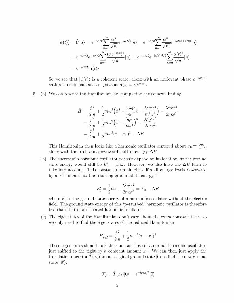
So we see that |ψ(t)〉 is a coherent state, along with an irrelevant phase e−iωt/2,with a time-dependent a eigenvalue α(t) ≡ αe−iωt.

5. (a) We can rewrite the Hamiltonian by ‘completing the square’, finding

H ′ =p2

2m+

1

2mω2

(

x2 − 2λqǫ

mω2x+

λ2q2ǫ2

m2ω4

)

− λ2q2ǫ2

2mω2

=p2

2m+

1

2mω2

(

x− λqǫ

mω2

)2

− λ2q2ǫ2

2mω2

=p2

2m+

1

2mω2(x− x0)

2 −∆E

This Hamiltonian then looks like a harmonic oscillator centered about x0 ≡ λqǫmω2 ,

along with the irrelevant downward shift in energy ∆E.

(b) The energy of a harmonic oscillator doesn’t depend on its location, so the groundstate energy would still be E ′

0 = 12~ω. However, we also have the ∆E term to

take into account. This constant term simply shifts all energy levels downwardby a set amount, so the resulting ground state energy is

E ′0 =

1

2~ω − λ2q2ǫ2

2mω2= E0 −∆E

where E0 is the ground state energy of a harmonic oscillator without the electricfield. The ground state energy of this ‘perturbed’ harmonic oscillator is thereforeless than that of an isolated harmonic oscillator.

(c) The eigenstates of the Hamiltonian don’t care about the extra constant term, sowe only need to find the eigenstates of the reduced Hamiltonian

H ′red =

p2

2m+

1

2mω2(x− x0)

2

These eigenstates should look the same as those of a normal harmonic oscillator,just shifted to the right by a constant amount x0. We can then just apply thetranslation operator T (x0) to our original ground state |0〉 to find the new groundstate |0′〉,

|0′〉 = T (x0)|0〉 = e−ipx0/~|0〉

5

where the value of x0 just comes from the Hamiltonian,

x0 =λqǫ

mω2

The full form of the ground state is therefore

|0′〉 = e−ipλqǫ/mω2~|0〉

(d) The only piece that depends on λ is the exponential out front, so we can expandthat out

e−ipλqǫ/mω2~ ≈ I − iλqǫ

mω2~p = I − λqǫ√

2mω3~(a− a†)

Acting with this operator on the original ground state, we find

|0′〉 ≈(

I − λqǫ√2mω3~

(a− a†))

|0〉 = |0〉+ λqǫ√2mω3~

|1〉

So we see that our new ground state can be approximated as a linear combinationof the original ground and first excited states.

Turning to the expectation values, we have

〈x〉 = 〈0|eipx0/~xe−ipx0/~|0〉 ≈ 〈0|(I + ix0

~p)x(I − ix0

~p)|0〉

≈ 〈0|(

x+iλqǫ

mω2~(px− xp)

)

|0〉 = λqǫ

mω2= x0

〈p〉 = 〈0|eipx0/~pe−ipx0/~|0〉 ≈ 〈0|(I + ix0

~p)p(I − ix0

~p)|0〉

≈ 〈0|(

p+iλqǫ

mω2~(p2 − p2)

)

|0〉 = 0

Next we can consider

〈x2〉 = 〈0|eipx0/~x2e−ipx0/~|0〉 ≈ 〈0|(I + ix0

~p)x2(I − ix0

~p)|0〉

≈ 〈0|(

x2 +iλqǫ

mω2~(px2 − x2p)

)

|0〉 = ~

2mω

〈p2〉 = 〈0|eipx0/~p2e−ipx0/~|0〉 ≈ 〈0|(I + ix0

~p)p2(I − ix0

~p)|0〉

≈ 〈0|(

p2 +iλqǫ

mω2~(p3 − p3)

)

|0〉 = mω~

2

We can then find the uncertainties,

6

∆x ≈√

~

2mω

∆p ≈√

mω~

2

So we see that, to first order in λ, this system just seems like a harmonic oscillatorwhich has moved to the right by x0.

7